Simulação de colunas de destilação convencional, extrativa e azeotropica no processo de produção de bioetanol atraves da modelagem de não equilibrio e da modelagem de estagios

UNIVERSIDADE ESTADUAL DE CAMPINAS

FACULDADE DE ENGENHARIA QUÍMICA

ÁREA DE CONCENTRAÇÃO:

DESENVOLVIMENTO DE PROCESSOS QUÍMICOS

SIMULAÇÃO DE COLUNAS DE DESTILAÇÃO

CONVENCIONAL, EXTRATIVA E AZEOTRÓPICA NO

PROCESSO DE PRODUÇÃO DE BIOETANOL ATRAVÉS DA

MODELAGEM DE NÃO EQUILÍBRIO E DA MODELAGEM DE

ESTÁGIOS DE EQUILÍBRIO COM EFICIÊNCIA

Autora: Tassia Lopes Junqueira

Orientador: Prof. Dr. Rubens Maciel Filho

Co-orientadora: Prof.ª Dra. Maria Regina Wolf Maciel

Dissertação de Mestrado apresentada à Faculdade de Engenharia Química como parte

dos requisitos exigidos para a obtenção do título de Mestre em Engenharia Química.

Campinas - São Paulo Março de 2010

FICHA CATALOGRÁFICA ELABORADA PELA

BIBLIOTECA DA ÁREA DE ENGENHARIA E ARQUITETURA - BAE -

UNICAMP

J968s

Junqueira, Tassia Lopes

Simulação de colunas de destilação convencional,

extrativa e azeotrópica no processo de produção de

bioetanol através da modelagem de não equilíbrio e da

modelagem de estágios de equilíbrio com eficiência /

Tassia Lopes Junqueira. --Campinas, SP: [s.n.], 2010.

Orientadores: Rubens Maciel Filho, Maria Regina

Wolf Maciel.

Dissertação de Mestrado - Universidade Estadual de

Campinas, Faculdade de Engenharia Química.

1. Bioetanol. 2. Separação (Tecnologia). 3.

Destilação - Modelos matemáticos. 4. Termodinâmica

de sistemas em não-equilíbrio. 5. Simulação por

computador. I. Maciel Filho, Rubens. II. Maciel, Maria

Regina Wolf. III. Universidade Estadual de Campinas.

Faculdade de Engenharia Química. IV. Título.

Título em Inglês: Simulation of conventional, extractive and azeotropic

distillation for bioethanol production process using

nonequilibrium model and equilibrium stage model with

efficiency

Palavras-chave em Inglês: Bioethanol, Separation (Technology),

Distillation - Mathematical models, Non-

equilibrium thermodynamics, Computer

simulation

Área de concentração: Desenvolvimento de Processos Químicos

Titulação: Mestre em Engenharia Química

Banca examinadora: Antonio Maria Francisco Luiz Jose Bonomi, Carlos

Eduardo Vaz Rossell, Mario Eusébio Torres Alvarez

Data da defesa: 02/03/2010

Programa de Pós Graduação: Engenharia Química

i

ii

iii

Aos meus pais, Roberto e Mara,

pelo amor, compreensão e incentivo,

dedico este trabalho.

iv

Agradecimentos

É difícil demonstrar com palavras toda a gratidão que sinto por todos

aqueles que estiveram ao meu lado ao longo desta etapa tão importante da minha

vida, seja para suporte ao meu trabalho, seja para incentivo pessoal. Agradeço

verdadeiramente a todos. Em especial, meus agradecimentos:

A Deus que me guiou e me iluminou para seguir em frente independente de

qualquer dificuldade.

Aos meus pais, Roberto e Mara, por acreditarem em minha capacidade e

investirem em mim amor, tempo e esforços. À minha mãe agradeço ainda por me

ouvir incansavelmente, ajudando-me em cada decisão.

Aos meus irmãos, João Gustavo, Roberta e Maira, por todo o apoio e

carinho.

Ao meu namorado Raphael, pelo amor, incentivo e paciência e por estar

sempre ao meu lado.

Aos professores Rubens Maciel Filho e Maria Regina Wolf Maciel, pela

orientação, incentivo, dedicação e amizade ao longo deste trabalho.

Aos meus amigos, Carlos e Cecilia, pela amizade e nossos inesquecíveis

almoços.

À Marina pela ajuda no desenvolvimento deste trabalho e pela grande

amizade.

Ao Daniel pelas proveitosas discussões e por estar sempre disposto a

ajudar. E aos funcionários do CTC pelas colaborações a este trabalho.

À Usina da Pedra e seus funcionários pela recepção e dados fornecidos

para a execução deste trabalho.

Aos colegas do LOPCA/LDPS e à Cristiane e à Mara do LDPC.

Aos funcionários e professores da Faculdade de Engenharia Química da

Unicamp.

À FAPESP pelo apoio financeiro.

v

“Nunca duvide que um pequeno grupo de

pessoas determinadas possa mudar o mundo.

De fato, foi sempre assim que o mundo mudou”

Margaret Mead

“Se você acha que pode fazê-lo, isto é confiança.

Se você o fizer, isto é competência"

Ken Blanchard

vi

Resumo

No Brasil, o bioetanol é usado para substituir a gasolina, compondo uma

porcentagem desta ou sendo usado como combustível alternativo. Esta tendência

de substituição dos combustíveis fósseis vem se fortalecendo em âmbito global,

sendo necessárias, portanto, alternativas e propostas que viabilizem o aumento da

produção de forma economicamente e ambientalmente sustentável. Neste

contexto, a otimização energética do processo de separação do bioetanol visa à

disponibilização de bagaço de cana-de-açúcar, usado como combustível na

geração de vapor de processo, para a produção de bioetanol através do processo

de hidrólise. Para tanto, inovações ao processo são essenciais e melhoramento na

representação de modelos torna-se necessário para estudos e avaliações.

Neste trabalho, simulações da etapa de destilação para a produção de

álcool hidratado assim como da etapa de desidratação do bioetanol foram

realizadas utilizando o simulador Aspen Plus®. Visando um estudo dentro de um

cenário mais realista, a modelagem de estágios de não equilíbrio foi utilizada para

prever o comportamento das colunas de destilação envolvidas. Além disso, o uso

da correlação de Barros e Wolf para a determinação de eficiência na modelagem

de estágios de equilíbrio em colunas de destilação foi avaliado.

A comparação entre as modelagens de estágios de equilíbrio e não

equilíbrio para as destilações convencional e extrativa indicou que a associação

da correlação de eficiência de Barros e Wolf à modelagem de estágios de

equilíbrio fornece predições satisfatórias tendo como referência a modelagem de

estágios de não-equilíbrio. Para a destilação azeotrópica, o estudo de formação de

duas fases líquidas na coluna foi realizado, indicando que os parâmetros de

processo, como posição de alimentação, possuem influência significativa.

O estudo da fermentação extrativa a vácuo, como configuração alternativa

às etapas de fermentação e concentração, revelou seu potencial para redução do

consumo de energia na etapa de destilação subseqüente, sendo uma alternativa

viável para intensificação de processos.

Palavras-chave: Bioetanol, Separação, Destilação, Não-equilíbrio, Simulação

vii

Abstract

In Brazil, bioethanol is used to replace gasoline, being a percentage of this

or used as an alternative fuel. This trend of replacing fossil fuels has gained

strength globally, necessitating, therefore, alternatives and proposals to enable the

increase of production in an economically and environmentally sustainable way. In

this context, the energy optimization of the bioethanol separation aims the

provision of sugarcane bagasse, used as fuel in process steam generation, for

bioethanol production through the hydrolysis process. Consequently, innovations to

the process are essential and improvement in the representation of models is

required for studies and evaluations.

In this work, simulations of the distillation step for the production of hydrous

bioethanol and the bioethanol dehydration were performed using the simulator

Aspen Plus®. In order to study a more realistic scenario, nonequilibrium stage

model was used to predict the behavior of the involved distillation columns.

Furthermore, the use of Barros and Wolf correlation for the determination of

efficiency in equilibrium stage model for distillation columns was evaluated.

The comparison between equilibrium and nonequilibrium stage models for

conventional and extractive distillation processes indicated that the association

between Barros and Wolf efficiency correlation and equilibrium stage model

provides satisfactory predictions considering the nonequilibrium stage model as

reference. For azeotropic distillation, formation of two liquid phases inside the

column was studied, indicating that process parameters, such as feed position,

have significant influence.

The study of vacuum extractive fermentation, as an alternative configuration

to fermentation and concentration steps, showed its potential for reducing energy

consumption in the subsequent distillation step, and it seems a viable alternative to

process intensification.

Keywords: Bioethanol, Separation, Distillation, Nonequilibrium, Simulation

viii

Sumário

Resumo ................................................................................................................. vi

Abstract ................................................................................................................ vii

Lista de Figuras ..................................................................................................... x

Lista de Tabelas ................................................................................................ xvii

Nomenclatura ..................................................................................................... xix

Capítulo 1 - Introdução e Objetivos ..................................................................... 1

1.1. Introdução ................................................................................................. 1

1.2. Objetivos ................................................................................................... 2

1.3. Estrutura da Dissertação ........................................................................... 3

Capítulo 2 - Revisão da Literatura ....................................................................... 5

2.1. Etanol Combustível ................................................................................... 5

2.2. Processo de Obtenção do Bioetanol ......................................................... 7

2.3. Modelagem de Colunas de Destilação .................................................... 17

Capítulo 3 - Processos Eficientes de Separação Etanol – Água ..................... 23

3.1. Introdução ............................................................................................... 23

3.2. Improving sustainability of bioethanol production: efficient ethanol – water

separation processes ......................................................................................... 24

3.3. Comentários e Conclusões ..................................................................... 39

Capítulo 4 - Caracterização Termodinâmica ..................................................... 41

4.1. Introdução ............................................................................................... 41

4.2. Phase equilibrium data for binary mixtures in bioethanol production -

evaluation of thermodynamic models adequacy ................................................ 43


Capítulo 5 - Avaliação dos Métodos de Cálculo para a Destilação

Convencional na Produção de Bioetanol .......................................................... 55

5.1. Introdução ............................................................................................... 55

5.2. Bioethanol Production Process: assessment of different calculation

methods for conventional distillation .................................................................. 56


ix

Capítulo 6 - Avaliação dos Métodos de Cálculo para a Destilação Extrativa na

Produção de Bioetanol ....................................................................................... 74

6.1. Introdução ............................................................................................... 74

6.2. Simulation of extractive distillation process in bioethanol production using

equilibrium stage model with efficiency and nonequilibrium stage model .......... 75


Capítulo 7 - Simulação do Processo de Produção de Bioetanol usando

Correlações de Eficiência para Destilação Convencional e Extrativa ............ 90

7.1. Introdução ............................................................................................... 90

7.2. Simulation of Anhydrous Bioethanol Production Process using Efficiency

Correlations for Conventional and Extractive Distillation ................................... 90


Capítulo 8 - Simulação da Destilação Azeotrópica no Processo de Produção

de Bioetanol Anidro .......................................................................................... 101

8.1. Introdução ............................................................................................. 101

8.2. Simulation of the azeotropic distillation for anhydrous bioethanol

production: study on the formation of a second liquid phase ........................... 102

8.3. Comentários e Conclusões ................................................................... 109

Capítulo 9 - Simulação do Processo de Extração Fermentativa a Vácuo e

Análise do Impacto na Etapa de Destilação .................................................... 110

9.1. Introdução ............................................................................................. 110

9.2. Evaluation of an extractive fermentation process coupled with a vacuum

flash chamber and the subsequent distillation for bioethanol production ......... 110

9.3. Comentários e Conclusões ................................................................... 128

Capítulo 10 - Análise Geral dos Resultados ................................................... 129

10.1. Modelagem de Estágios de Equilíbrio ................................................... 129

10.2. Modelagem de Estágios de Não Equilíbrio ........................................... 130

10.3. Aplicação da Correlação de Eficiência .................................................. 131

Capítulo 11 - Conclusões e Sugestões para Trabalhos Futuros ................... 132

11.1. Conclusões ........................................................................................... 132

11.2. Sugestões para Trabalhos Futuros ....................................................... 133

Referências Bibliográficas ............................................................................... 135

Apêndice ............................................................................................................ 146

x

Lista de Figuras

Figura 2.1. Produção brasileira de etanol combustível entre as safras de 1997/98

e 2007/08. ............................................................................................................... 6

Figura 2.2. Diagrama de blocos do processo de produção de etanol anidro a partir

do caldo e do bagaço da cana-de-açúcar. .............................................................. 9

Figura 2.3. Configuração usual da destilação no processo de produção de

bioetanol. ............................................................................................................... 12

Figura 2.4. Configuração da destilação azeotrópica para produção de bioetanol

anidro. ................................................................................................................... 14

Figura 2.5. Configuração usual da destilação extrativa. ........................................ 16

Figure 3.1. Configuration of the conventional distillation process. .......................... 27

Figure 3.2. Configuration of the azeotropic distillation process for anhydrous

bioethanol production.. ........................................................................................... 28

Figure 3.3. Configuration of conventional (a) and alternative (b) extractive distillation

process for anhydrous bioethanol production.. ........................................................ 29

Figure 3.4: Example of extractive distillation process configuration with non-volatile

entrainers Ionic Liquid (IL) or low-viscosity Hyperbranched Polymers (HyPol). ........ 31

Figure 3.5. Configuration of the adsorption onto molecular sieves process for

anhydrous bioethanol production.. .......................................................................... 32

Figure 3.6. Configuration of the pervaporation process for anhydrous bioethanol

production. ............................................................................................................. 33

Figure 4.1. T-x-y diagram for the ethanol (1) - water (2) system, at 760 mm Hg. . 46

Figure 4.2. T-x diagram for the sucrose (1) - water (2) system, at 760 mm Hg. .... 48

Figure 4.3. T-x-y diagram for the acetic acid (1) - furfural (2) system, at 667 mm

Hg. ......................................................................................................................... 49

Figure 4.4. T-x-y diagram for the water (1) - glycerol (2) system, at 760 mm Hg. . 49

xi

Figure 4.5. Ternary diagram for the ethanol – water - cyclohexane system, at 760

mmHg and 35 ºC. .................................................................................................. 52

Figure 4.6. T-x-y diagram for the water (1) – MEG (2) system, at 760 mmHg. ...... 52

Figure 4.7. T-x-y diagram for the ethanol (1) – MEG (2) system, at 760 mmHg. ... 53

Figure 5.1. Configuration of the simulated process. .............................................. 59

Figure 5.2. Isoamyl alcohol mass fraction profile in column B-B1 for equilibrium

model simulation. .................................................................................................. 63

Figure 5.3. Temperature profile for column B-B1 using nonequilibrium stage

model. ................................................................................................................... 65

Figure 5.4. Temperature profile using equilibrium stage model with constant plate

efficiencies and nonequilibrium stage model. ........................................................ 65

Figure 5.5. Comparison between energy demand of distillation process using

equilibrium stage model with constant plate efficiencies and nonequilibrium stage

model. ................................................................................................................... 66

Figure 5.6. Efficiency profile in column B-B1. ........................................................ 67

Figure 5.7. Temperature profile using equilibrium model with Barros & Wolf

efficiency correlation for plate and component and nonequilibrium stage model... 68


equilibrium model with Barros & Wolf efficiency correlation for plate and component

and nonequilibrium model. .................................................................................... 69

Figure 5.9. Composition profile for vapor phase considering equilibrium model with

efficiency of 100 %, with efficiency estimated by Barros & Wolf correlation and

nonequilibrium stage model................................................................................... 70

Figure 5.10. Composition profile for liquid phase considering equilibrium model with


nonequilibrium model. ........................................................................................... 70

Figure 6.1. Configuration of extractive distillation process with ethyleneglycol. .... 80

Figure 6.2. Efficiency profiles obtained in the extractive column. .......................... 84

Figure 6.3. Temperature profiles in extractive column. .......................................... 84

xii

Figure 6.4. Composition profiles for vapor phase in extractive column. ................ 85

Figure 6.5. Efficiency profiles obtained in the recovery column. ............................ 86

Figure 6.6. Temperature profiles in recovery column. ........................................... 87

Figure 6.7. Composition profiles for vapor phase in recovery column. .................. 87

Figure 7.1. Configuration of the conventional distillation process. ......................... 92

Figure 7.2. Configuration of extractive distillation process. ................................... 93

Figure 7.3. Efficiency profiles obtained in the columns. ......................................... 96

Figure 7.4. Temperature profile for column B-B1. ................................................. 98

Figure 7.5. Temperature profile for the extractive column (EC). ............................ 98

Figure 8.1. First configuration of the azeotropic distillation process. ................... 104

Figure 8.2. Second configuration of the azeotropic distillation process. .............. 105

Figure 8.3. Third configuration of the azeotropic distillation process. .................. 105

Figure 8.4. Liquid flow profile in the azeotropic column for configuration 1. ........ 108



Figure 9.1. Configuration of the conventional fermentation process. ................... 114

Figure 9.2. Configuration of the vacuum extractive fermentative process. .......... 115

Figure 9.3. Configuration of the conventional distillation process. ....................... 117

Figure 9.4. Configuration of the double effect distillation process. ...................... 118

Figure 9.5. Configuration of the triple effect distillation. ....................................... 119

Figure 9.6. Analysis of the flash chamber conditions: outlet temperature of the flash

chamber and ethanol content of the flash vapor phase for different vessel

pressures............................................................................................................. 120

Figure 9.7. Recirculation flow and energy consumption for the main cases. ....... 122

Figura A.1. Diagrama y-x acetaldeído (1) / acetona (2). ...................................... 146

Figura A.2. Diagrama y-x acetaldeído (1) / metanol (2). ...................................... 146

Figura A.3. Diagrama y-x acetaldeído (1) / acetato de etila (2). .......................... 146

xiii

Figura A.4. Diagrama y-x acetaldeído (1) / etanol (2). ......................................... 146

Figura A.5. Diagrama y-x acetaldeído (1) / n-propanol (2). ................................. 147

Figura A.6. Diagrama y-x acetaldeído (1) / água (2). ......................................... 147

Figura A.7. Diagrama y-x acetaldeído (1) / isobutanol (2). .................................. 147

Figura A.8. Diagrama y-x acetaldeído (1) / ácido acético (2)............................... 147

Figura A.9. Diagrama y-x acetaldeído (1) / n-butanol (2). ................................... 147

Figura A.10. Diagrama y-x acetaldeído (1) / álcool Isoamílico (2). ...................... 147

Figura A.11. Diagrama y-x acetaldeído (1) / furfural (2) ...................................... 148

Figura A.12. Diagrama y-x acetaldeído (1) / glicerol (2). ..................................... 148

Figura A.13. Diagrama y-x acetaldeído (1) / glicose (2). ..................................... 148

Figura A.14.Diagrama y-x acetaldeído (1) / sacarose (2). ................................... 148

Figura A.15.Diagrama y-x acetona (1)/ metanol (2). ........................................... 148

Figura A.16.Diagrama y-x acetona (1) / acetato de etila (2). ............................... 148

Figura A.17. Diagrama y-x acetona (1) / etanol (2). ............................................ 149

Figura A.18. Diagrama y-x acetona (1) / n-propanol (2). ..................................... 149

Figura A.19. Diagrama y-x acetona (1) / água (2). ............................................. 149

Figura A.20. Diagrama y-x acetona (1) / isobutanol (2). ...................................... 149

Figura A.21. Diagrama y-x acetona (1) / ácido acético (2). ................................. 149

Figura A.22. Diagrama y-x acetona (1) / n-butanol (2). ....................................... 149

Figura A.23. Diagrama y-x acetona (1) / álcool isoamílico (2). ............................ 150

Figura A.24. Diagrama y-x acetona (1) / furfural (2). ........................................... 150

Figura A.25. Diagrama y-x acetona (1) / glicerol (2). ........................................... 150

Figura A.26. Diagrama y-x acetona (1) / glicose (2). ........................................... 150

Figura A.27. Diagrama y-x acetona (1) / sacarose (2). ........................................ 150

Figura A.28. Diagrama y-x metanol (1) / acetato de etila (2) ............................... 150

Figura A.29. Diagrama y-x metanol (1) / etanol (2) ............................................. 151

Figura A.30. Diagrama y-x metanol (1) / n-propanol (2). ..................................... 151

xiv

Figura A.31. Diagrama y-x metanol (1) / água (2). ............................................. 151

Figura A.32. Diagrama y-x metanol (1) / isobutanol (2). ...................................... 151

Figura A.33. Diagrama y-x metanol (1) / ácido acético (2). ................................. 151

Figura A.34. Diagrama y-x metanol (1) / n-butanol (2). ....................................... 151

Figura A.35. Diagrama y-x metanol (1) / álcool isoamílico (2). ............................ 152

Figura A.36. Diagrama y-x metanol (1) / furfural (2). ........................................... 152

Figura A.37. Diagrama y-x metanol (1) / glicerol (2). ........................................... 152

Figura A.38. Diagrama y-x metanol (1) / glicose (2). ........................................... 152

Figura A.39. Diagrama y-x metanol (1) / sacarose (2). ........................................ 152

Figura A.40. Diagrama y-x acetato de etila (1) / etanol (2). ................................. 152

Figura A.41. Diagrama y-x acetato de etila (1) / n-propanol (2). .......................... 153

Figura A.42. Diagrama y-x acetato de etila (1) / água (2). ................................... 153

Figura A.43. Diagrama y-x acetato de etila (1) / isobutanol (1). .......................... 153

Figura A.44. Diagrama y-x acetato de etila (1) / ácido acético (2). ...................... 153

Figura A.45. Diagrama y-x acetato de etila (1) / n-butanol (2). ............................ 153

Figura A.46. Diagrama y-x acetato de etila (1) / álcool isoamílico (2). ................ 153

Figura A.47. Diagrama y-x acetato de etila (1) / furfural (2)................................. 154

Figura A.48. Diagrama y-x acetato de etila (1) / glicerol (2). ............................... 154

Figura A.49. Diagrama y-x com acetato de etila (1) / glicose (2). ........................ 154

Figura A.50. Diagrama y-x acetato de etila (1) / sacarose (2). ............................ 154

Figura A.51. Diagrama y-x etanol (1) / n-propanol (2). ........................................ 154

Figura A.52. Diagrama y-x etanol (1) / água (2). ................................................. 154

Figura A.53. Diagrama y-x etanol (1) / isobutanol (2). ......................................... 155

Figura A.54. Diagrama y-x etanol (1) / ácido acético (2). .................................... 155

Figura A.55. Diagrama y-x etanol (1) / n-butanol (2). .......................................... 155

Figura A.56. Diagrama y-x etanol (1) / álcool isoamílico (2). ............................... 155

Figura A.57. Diagrama y-x etanol (1) / furfural (2). .............................................. 155

xv

Figura A.58. Diagrama y-x etanol (1) / glicerol (2). .............................................. 155

Figura A.59. Diagrama y-x etanol (1) / glicose (2). .............................................. 156

Figura A.60. Diagrama y-x etanol (1) / sacarose (2). ........................................... 156

Figura A.61. Diagrama y-x n-propanol (1) / água (2). .......................................... 156

Figura A.62. Diagrama y-x n-propanol (1) / isobutanol (2). ................................. 156

Figura A.63. Diagrama y-x n-propanol (1) / ácido acético (2). ............................. 156

Figura A.64. Diagrama y-x n-propanol (1) / n-butanol (2). .................................. 156

Figura A.65. Diagrama y-x n-propanol (1) / álcool isoamílico (2). ........................ 157

Figura A.66. Diagrama y-x n-propanol (1) / furfural (2). ....................................... 157

Figura A.67. Diagrama y-x n-propanol (1) / glicerol (2). ...................................... 157

Figura A.68. Diagrama y-x n-propanol (1) / glicose (2). ....................................... 157

Figura A.69. Diagrama y-x n-propanol (1) / sacarose (1). ................................... 157

Figura A.70. Diagrama y-x água (1) / isobutanol (2). ........................................... 157

Figura A.71. Diagrama y-x água (1) / ácido acético (2). ...................................... 158

Figura A.72. Diagrama y-x água (1) / n-butanol (2). ............................................ 158

Figura A.73. Diagrama y-x água (1) / álcool isoamílico (2). ................................. 158

Figura A.74. Diagrama y-x água (1) / furfural (2). ................................................ 158

Figura A.75. Diagrama y-x água (1) / glicerol (2). ................................................ 158

Figura A.76. Diagrama y-x água (1) / glicose (2). ................................................ 158

Figura A.77. Diagrama y-x água (1) / sacarose (2). ............................................ 159

Figura A.78. Diagrama y-x isobutanol (1) / ácido acético (2). .............................. 159

Figura A.79. Diagrama y-x isobutanol (1) / n-butanol (2). .................................... 159

Figura A.80. Diagrama y-x isobutanol (1) / álcool isoamílico (2). ........................ 159

Figura A.81. Diagrama y-x isobutanol (1) / furfural (2). ....................................... 159

Figura A.82. Diagrama y-x isobutanol (1) / glicerol (2). ....................................... 159

Figura A.83. Diagrama y-x isobutanol (1) / glicose (2). ....................................... 160

Figura A.84. Diagrama y-x isobutanol (1) / sacarose (2). .................................... 160

xvi

Figura A.85. Diagrama y-x ácido acético (1) / n-butanol (2). ............................... 160

Figura A.86. Diagrama y-x ácido acético (1) / álcool isoamílico (2). .................... 160

Figura A.87. Diagrama y-x ácido acético (1) / furfural (2). ................................... 160

Figura A.88. Diagrama y-x ácido acético (1) / glicerol (2). ................................... 160

Figura A.89. Diagrama y-x ácido acético (1) / glicose (2). ................................... 161

Figura A.90. Diagrama y-x ácido acético (1) / sacarose (2). ............................... 161

Figura A.91. Diagrama y-x n-butanol (1) / álcool isoamílico (2). .......................... 161

Figura A.92. Diagrama y-x n-butanol (1) / furfural (2). ......................................... 161

Figura A.93. Diagrama y-x n-butanol (1) / glicerol (2). ......................................... 161

Figura A.94. Diagrama y-x n-butanol (1) / glicose (2). ......................................... 161

Figura A.95. Diagrama y-x n-butanol (1) / sacarose (2). ..................................... 162

Figura A.96. Diagrama y-x álcool isoamílico (1) / furfural (2)............................... 162

Figura A.97. Diagrama y-x álcool isoamílico (1) / glicerol (2). ............................. 162

Figura A.98. Diagrama y-x álcool isoamílico (1) / glicose (2)............................... 162

Figura A.99. Diagrama y-x álcool isoamílico (1) / sacarose (2). .......................... 162

Figura A.100. Diagrama y-x furfural (1) / glicerol (2). .......................................... 162

Figura A.101. Diagrama y-x furfural (1) / glicose (2). ........................................... 163

Figura A.102. Diagrama y-x furfural (1) / sacarose (2). ....................................... 163

Figura A.103. Diagrama y-x glicerol (1) / glicose (2). .......................................... 163

Figura A.104. Diagrama y-x glicerol (1) / sacarose (2). ....................................... 163

Figura A.105. Diagrama y-x glicose (1) / sacarose (2). ....................................... 163

Figura A.106. Diagrama y-x etanol (1) / cicloexano (2). ...................................... 163

Figura A.107. Diagrama y-x cicloexano (1) / água (2). ........................................ 164

Figura A.108. Diagrama y-x etanol (1) / etilenoglicol (2). .................................... 164

Figura A.109. Diagrama y-x água (1) / etilenoglicol (2). ...................................... 164

xvii

Lista de Tabelas

Tabela 3.1. Comparação entre os processos apresentados. ................................ 40

Tabela 4.1. Temperaturas de ebulição dos componentes envolvidos no processo

de produção de bioetanol a pressão atmosférica. ................................................. 42

Table 4.2. Sources for the binary pairs equilibrium data. ...................................... 45

Table 4.3. Representative model for each binary. ................................................. 47

Table 4.4. Behavior of selected binary pairs.......................................................... 50

Table 5.1. Distillation columns conditions and specifications ................................ 60

Table 5.2. Composition of wine fed to distillation process. .................................... 61

Table 5.3. Main stream results given by nonequilibrium model. ............................ 64

Table 5.4. Comparison between energy requirements. ......................................... 71

Table 6.1. Specifications in the extractive and recovery columns (mass basis). ... 80

Table 6.2. Main stream results using nonequilibrium stage model. ......................... 81

Table 6.3. Main stream results using equilibrium stage model. ............................... 82

Table 6.4. Main stream results using equilibrium stage model with plate efficiency. 82

Table 6.5. Main stream results using equilibrium stage model with component

efficiency. ............................................................................................................... 82

Table 6.6. Energy requirements for all calculation methods. ................................. 83

Table 7.1. Composition of the streams fed to the process. ................................... 95

Table 7.2. Column specifications in bioethanol production process. ..................... 96

Table 7.3 Specifications in the extractive and recovery columns (mass basis). .... 96

Table 7.4. Stream for hydrous bioethanol production. ........................................... 97

Table 7.5 Stream for anhydrous bioethanol production. ........................................ 97

Table 8.1. Process parameters for each configuration. ....................................... 106

Table 8.2. Composition of the main streams for the first configuration. ............... 106

Table 8.3. Composition of the main streams for the second configuration. ......... 106

xviii

Table 8.4. Composition of the main streams for the third configuration. .............. 107

Table 8.5. Ethanol and entrainer losses and energy consumption on column

reboilers for each configuration. .......................................................................... 107

Table 9.1. Results obtained for different inlet temperatures and vessel

pressures............................................................................................................. 121

Table 9.2. Items present on each of the studied configurations. ......................... 123

Table 9.3. Parameters of the distillation columns. ............................................... 124

Table 9.4. Energy consumption on each configuration. ....................................... 125

Table 9.5. Energy consumption on each configuration, for the case of an annexed

distillery (use of sugar molasses as raw material). .............................................. 125

Table 9.6. Flow of the main process streams and ethanol losses on each

configuration. ....................................................................................................... 126

Tabela 10.1. Energias requeridas em cada processo. ........................................ 129

Tabela A.1. Não idealidades observadas no sistema. ......................................... 165

xix

Nomenclatura

Letras Latinas

D Difusividade, [m2 s-1]

i Indica o estágio

I Interface

j Indica o componente

k Condutividade térmica, [W m-1 K-1]

L Fase líquida

T Temperatura, [ºC]

V Fase vapor

x Fração molar na fase líquida

y Fração molar na fase vapor

Letras Gregas

µ Viscosidade, [Pa s]

η Eficiência de Murphree

ρ Massa específica, [kg m-3]

Siglas, Abreviações e Definições

AEAC/AE Álcool etílico anidro carburante

AEHC/HE Álcool etílico hidratado carburante

CFD Fluidodinâmica Computacional

comp Componente

Cp Capacidade calorífica, [J kmol-1 K-1]

xx

EC Coluna de Destilação Extrativa

Eff Eficiência

HMF 5-hydroxymethyl-furfural

HOC Correlação de Hayden-O’Connell

HyPol Polímeros altamente ramificados

IL Líquidos iônicos

MEG / EG Monoetilenoglicol

MW Massa molecular, [kg kmol-1]

nc Número de componentes

NRTL Non-Random Two-Liquid, modelo para o cálculo de coeficiente de

atividade

RC Coluna de recuperação de solvente

UNIFAC UNIQUAC Functional-group Activity Coefficient, método de cálculo de

coeficiente de atividade

UNIQUAC

Universal Quasi-Chemical, modelo para o cálculo de coeficiente de

atividade

VLE Equilíbrio líquido-vapor

1

Capítulo 1

Introdução e Objetivos

1.1. Introdução

Devido às atuais preocupações acerca do aquecimento global e aos novos

contratos internacionais de produção de bioetanol, espera-se que a indústria

alcooleira seja um dos propulsores da economia brasileira nos próximos anos.

Embora a produção em grande escala deste combustível já dure mais de 30 anos,

melhorias no processo devem ser buscadas para que o Brasil não perca a posição

que ocupa no cenário mundial com relação à produção de bioetanol (segundo

maior produtor mundial e maior exportador).

Além disso, a introdução dos veículos com motores bicombustíveis na frota

brasileira aumentou consideravelmente a demanda de álcool combustível. Neste

contexto, dois grandes desafios foram originados: manter os preços competitivos

frente à gasolina e motivar os produtores de álcool e açúcar a priorizar a produção

de bioetanol e assim manter o estoque deste e, consequentemente, os preços

atraentes no momento da escolha do combustível a ser abastecido.

Dessa forma, para atender à demanda nacional e mundial, o Brasil

necessita aumentar a sua produção de bioetanol e também diminuir os custos de

produção. Diferentemente dos Estados Unidos, o Brasil possui grande potencial

para atingir estes objetivos, uma vez que, além de utilizar a matéria-prima mais

eficiente (cana-de-açúcar), apresenta excesso de bagaço e palha. Estes

subprodutos podem ser utilizados na produção de vapor e energia elétrica através

da queima em caldeiras, permitindo que as usinas sejam auto-suficientes em

energia elétrica e, nos casos de utilização de sistemas eficientes de cogeração,

vendam energia elétrica às concessionárias.

Outra vantagem competitiva do país é sua grande disponibilidade de áreas

apropriadas para o cultivo de cana-de-açúcar, sendo possível a expansão agrícola

sem afetar áreas ambientalmente preservadas e sem ocorrer competição com a

agricultura de alimentos.

2

Adicionalmente, novos desenvolvimentos no processo de produção de

bioetanol como a viabilização da hidrólise de materiais lignocelulósicos (por

exemplo, o bagaço e a palha da cana) para produção de álcool de segunda

geração e novas rotas de produção como a conversão de gás de síntese em

bioetanol vêm sendo investigados no país.

Vale ressaltar que, independentemente da rota utilizada para a obtenção de

bioetanol, o bioetanol é obtido em baixas concentrações, geralmente diluído em

água e co-produtos, sendo assim as etapas de concentração e desidratação são

de grande importância no processo de produção de bioetanol. Com esta finalidade

são comumente empregadas colunas de destilação, cujas variáveis operacionais

influenciam fortemente no consumo de vapor de processo. Como consequência da

redução no consumo de vapor, menos bagaço de cana-de-açúcar precisa ser

queimado a fim de fornecer energia à planta, aumentando, portanto, a quantidade

de bagaço disponível para a cogeração de energia elétrica e para o processo de

produção de álcool de segunda geração, que possibilita o aumento de produção

sem acrescer a área plantada.

Além da aplicação como combustível, o bioetanol também pode ser

utilizado como matéria-prima na produção de diferentes produtos químicos

produzidos normalmente a partir de derivados de petróleo, como o eteno. O

aumento nos preços do petróleo motiva também o desenvolvimento de rotas de

produção alternativas para este e outros petroquímicos básicos, sendo a

alcoolquímica uma alternativa cada vez mais atraente (Dias, 2008).

1.2. Objetivos

Diante da variada gama de utilização do bioetanol, o aumento da produção,

sem acrescer proporcionalmente as áreas de cultivo, é um grande desafio.

Portanto, a melhoria da eficiência do processo de produção de bioetanol é

essencial e o estudo de cada etapa do processo é necessário.

Neste contexto, o objetivo geral deste trabalho é a simulação das etapas de

concentração e desidratação do processo de produção de bioetanol, de forma

mais realista possível, através do simulador Aspen Plus®. Para tanto, a

3

modelagem de estágios de não equilíbrio é empregada e sua comparação à

modelagem de estágios de equilíbrio serve como base para o estabelecimento de

uma metodologia mais confiável para prever a eficiência de estágio.

Assim, foram determinados os seguintes objetivos específicos:

definição do modelo termodinâmico mais representativo do sistema;

simulação dos processos de destilação convencional e extrativa

utilizando a modelagem de estágios de equilíbrio, aplicação da

correlação de eficiência e modelagem de estágios de não equilíbrio;

simulação da destilação azeotrópica visando à diminuição da região de

duas fases líquidas no interior da coluna;

proposição de configuração alternativa para o processo de destilação.

1.3. Estrutura da Dissertação

Esta dissertação é dividida em 11 capítulos da seguinte forma:

No Capítulo 2, a revisão da literatura é apresentada, sendo salientada a

importância do bioetanol como combustível e apresentada a descrição do

processo de produção de bioetanol. São também abordadas as modelagens para

colunas de destilação bem como os conceitos e correlações de eficiência.

No Capítulo 3 é apresentada uma revisão dos processos de separação

atualmente empregados no processo de produção de bioetanol bem como dos

recentes desenvolvimentos nesta área.

A caracterização termodinâmica do sistema é apresentada no Capítulo 4.

Neste capítulo são avaliados modelos de coeficiente de atividade para a fase

líquida através da comparação com dados experimentais de equilíbrio líquido-

vapor e líquido-líquido dos binários presentes no sistema.

Resultados das simulações utilizando modelagens de estágios de equilíbrio,

não equilíbrio e equilíbrio com eficiência são apresentados e comparados no

Capítulo 5 para o processo de destilação convencional empregado para a

produção de álcool hidratado.

4

No Capítulo 6, modelagens de estágios de equilíbrio, não equilíbrio e

equilíbrio com eficiência são aplicadas para a simulação do processo de

destilação extrativa com monoetilenoglicol.

No Capítulo 7, simulações em conjunto das destilações convencional e

extrativa utilizando modelagem de estágios de equilíbrio e aplicação de

correlações de eficiência são apresentadas.

No Capítulo 8, diferentes configurações do processo de destilação

azeotrópica com cicloexano são avaliadas e otimizadas a fim de minimizar a

formação de duas fases líquidas na coluna, as perdas de produto e a demanda

energética.

Alternativas para as etapas de fermentação e destilação são apresentadas

no Capítulo 9. São apresentadas simulações do processo alternativo de

fermentação acoplado a diferentes configurações de destilação (convencional,

duplo e triplo efeito).

Análise geral dos resultados apresentados nesta dissertação é realizada no

Capítulo 10, de forma a comparar os diferentes processos estudados.

Finalmente, no Capítulo 11 são apresentadas as conclusões obtidas neste

trabalho bem como sugestões para trabalhos futuros.

Nesta dissertação de mestrado, o desenvolvimento dos capítulos

apresenta-se através de trabalhos submetidos, aceitos e/ou publicados em anais

de congressos, além de artigos a serem submetidos a periódicos.

5

Capítulo 2

Revisão da Literatura

2.1. Etanol Combustível

O uso de energia renovável tem sido visto como uma solução para as

questões relacionadas à poluição atmosférica e à escassez dos combustíveis

fósseis. Dessa forma, a conversão de biomassa em biocombustíveis representa

uma importante opção para aproveitamento de um recurso alternativo de energia e

para a redução da emissão de gases poluentes, principalmente de gás carbônico.

Atualmente, dois tipos de biocombustíveis são produzidos em larga escala:

bioetanol e biodiesel. A maior parte do bioetanol é produzida a partir de milho nos

Estados Unidos e de cana-de-açúcar no Brasil, enquanto menores quantidades

são obtidas na Europa tendo como matéria-prima o trigo e a beterraba. O biodiesel

é predominantemente produzido a partir de óleo de canola na Europa, de palma

na Ásia e de soja no Brasil (Goldemberg, 2008).

A adição de bioetanol à gasolina eleva o teor de oxigênio desta e,

consequentemente, permite uma melhor oxidação dos hidrocarbonetos e reduz a

quantidade de gases poluentes liberados para a atmosfera (Alzate e Toro, 2006).

Além disso, o bioetanol pode ser usado em substituição à gasolina, sendo que sua

combustão gera emissões de hidrocarbonetos menos tóxicas do que as da

gasolina, pois possuem menor reatividade atmosférica (Goldemberg et al., 2008a).

A fim de avaliar as vantagens em substituir a gasolina por bioetanol, alguns

estudos apresentam a análise do ciclo de vida do bioetanol. Balanços de energia e

de emissões de gases do efeito estufa mostraram-se bastante favoráveis para o

bioetanol derivado de cana-de-açúcar produzido no Brasil, mesmo quando este é

exportado para outros países (Goldemberg et al., 2008a).

No Brasil, o incentivo à produção de bioetanol iniciou-se na década de 70.

Com o Proálcool, programa de forte cunho estatal, o país tornou-se o maior

produtor de bioetanol do mundo até início de 2000, quando os Estados Unidos

ultrapassaram o Brasil. Isto porque com o objetivo primário de reduzir a

dependência estrangeira de derivados de petróleo e diminuir a emissão de gases

6

responsáveis pelo efeito estufa, os Estados Unidos impulsionaram de forma

expressiva o mercado mundial de bioetanol. No entanto, o Brasil continua sendo o

maior exportador mundial, uma vez que sua produção gera excedentes que

podem ser direcionados a outros países e também por possuir os menores custos

de produção (Souza, 2006).

Basicamente, o álcool combustível pode ser utilizado em duas formas:

anidro e hidratado; ambos são combustíveis usados em veículos de passeio e

comerciais leves, mas diferem quanto a sua forma de utilização. O álcool anidro,

ou álcool etílico anidro carburante (AEAC), é praticamente puro, com um teor

alcoólico entre 99,3 e 99,8 %. É utilizado como um aditivo que aumenta o teor de

oxigenados na gasolina. No Brasil, a porcentagem de álcool anidro na mistura

pode variar entre 20 e 25 %. O álcool hidratado, ou álcool etílico hidratado

carburante (AEHC), com teor entre 92,6 e 93,8 % em massa de etanol (BRASIL,

2005), pode ser utilizado diretamente em motores movidos a álcool ou

bicombustíveis (flex-fuel). Os veículos com motores flexíveis foram introduzidos no

mercado em março de 2003 e permitem o abastecimento, na sua totalidade, com

álcool hidratado ou gasolina, ou ainda, com qualquer teor de mistura desses

combustíveis (Scandiffio, 2005).

A Figura 2.1 apresenta a produção de álcool combustível no Brasil nos

últimos dez anos, utilizando dados fornecidos por MAPA (2009).

Figura 2.1. Produção brasileira de etanol combustível entre as safras de 1997/98 e

2007/08.

0,0

5,0

10,0

15,0

20,0

25,0

97/98 98/99 99/00 00/01 01/02 02/03 03/04 04/05 05/06 06/07 07/08

Safra

Pro

du

çã

o (

10

6 m

³)

AEHC AEAC

7

Observa-se que, a partir de 2003, em decorrência do lançamento dos

veículos flex-fuel, a produção de álcool hidratado tem aumentado

significativamente, superando a produção de álcool anidro desde 2005/06. A

produção total de álcool na safra de 2007/08, máxima no período compreendido,

foi de 22,2 milhões de metros cúbicos.

Além do grande potencial como combustível, o bioetanol possui diversas

aplicações nos setores farmacêutico, alimentício e químico, entre outros. A partir

de bioetanol é possível obter acetaldeído de alta qualidade, ácido acético, acetato

de etila, etileno e, a partir destes, uma grande variedade de produtos químicos,

incluindo polímeros (Rivera et al., 2008). Dessa forma, a utilização do bioetanol

como matéria-prima na produção de diferentes produtos químicos, produzidos

normalmente a partir de derivados do petróleo, surge como uma alternativa cada

vez mais atraente, principalmente por ser uma tecnologia sustentável, seguindo a

tendência da Engenharia Verde (Green Process Engineering).

2.2. Processo de Obtenção do Bioetanol

No Brasil, a matéria-prima empregada para a produção de bioetanol é a

cana-de-açúcar. Altamente eficiente e com baixo custo, o bioetanol de cana-de-

açúcar é uma das melhores opções para mitigar as emissões de gases de efeito

estufa decorrentes da queima de combustíveis fósseis (Goldemberg et al., 2008b).

Além disso, a cogeração de energia a partir do bagaço de cana permite que as

usinas sejam auto-suficientes em energia térmica e elétrica, além da possibilidade

de venda da eletricidade excedente (Ensinas, 2008).

Alternativamente ao uso do caldo de cana-de-açúcar, podem ser utilizados

para a produção de bioetanol outros recursos biológicos, como cultivos ricos em

energia (como o milho) ou de biomassa lignocelulósica, os quais requerem o

condicionamento ou pré-tratamento da matéria-prima para que os organismos de

fermentação convertam esta em etanol (Cardona e Sánchez, 2007). A chamada

biomassa lignocelulósica inclui resíduos agriculturais, agroindustriais, industriais

(processamento de alimentos e outros) e resíduos sólidos municipais. Dessa

forma, é uma matéria-prima bastante abundante, presente em materiais como:

8

bagaço de cana-de-açúcar, lascas de madeira, serragem, resíduos de papéis e

capim (Alzate e Toro, 2006).

A utilização do bagaço de cana como matéria-prima tem como vantagem

sua disponibilidade nas usinas e o aproveitamento de parte da infra-estrutura já

existente nestas (fermentação e separação). O bagaço da cana-de-açúcar é

composto principalmente pelos polímeros de carboidratos lignina (cerca de 20 %),

celulose (40 %) e hemicelulose (38 %) (IPT, 2000). Para a produção de bioetanol

é necessário transformar os polímeros em carboidratos fermentescíveis. A fração

hemicelulósica é facilmente convertida a pentoses e hexoses, mas no caso da

celulose é necessário realizar um tratamento prévio (Zaldivar et al., 2001),

utilizando-se um solvente para dissolver a lignina, permitindo assim a conversão

da celulose a hexoses utilizando catalisadores ácidos (hidrólise ácida) ou

enzimáticos (hidrólise enzimática). A hidrólise do bagaço permite o aumento

significativo da produção de bioetanol sem o aumento da área plantada de cana-

de-açúcar.

O processo de produção de bioetanol anidro é apresentado através de

diagrama de blocos na Figura 2.2, extraído de Dias (2008), que realizou a

simulação da produção de bioetanol a partir do caldo e do bagaço da cana-de-

açúcar, visando o levantamento do consumo de energia destes processos.

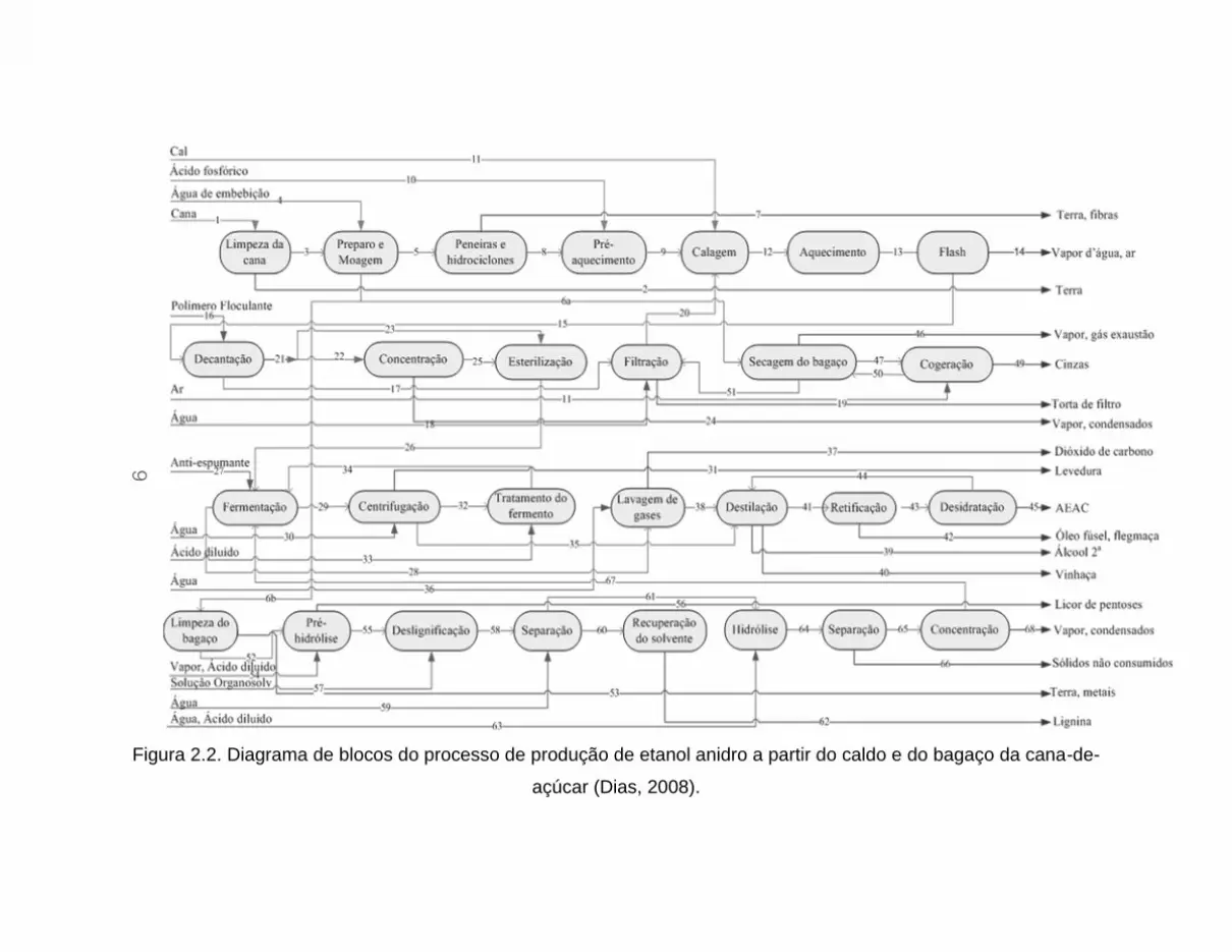
Figura 2.2. Diagrama de blocos do processo de produção de etanol anidro a partir do caldo e do bagaço da cana-de-

açúcar (Dias, 2008).

10

Dentre as etapas indicadas na Figura 2.2, neste trabalho são abordadas a

fermentação, a destilação e a desidratação, cujas descrições são apresentadas a

seguir.

2.2.1. Fermentação

A fermentação alcoólica consiste em uma série de reações químicas

catalisadas por um microorganismo, a levedura Saccharomyces cerevisiae. Essa

levedura é um aeróbio facultativo, isto é, pode se ajustar metabolicamente a

condições de aerobiose e anaerobiose. Enquanto porções de açúcar são

transformadas em biomassa (reprodução celular), H2O e CO2 em condições

aeróbias, a maior parte é convertida em etanol e CO2 em condições anaeróbias

(Lima et al., 2001). O produto da fermentação, denominado vinho, deve conter

entre 8 e 12 % (em massa) de etanol. Para obter um vinho final de graduação

elevada, é necessária uma fermentação estável com fermento ativo, livre de

inibição, infecção e floculação. Além disso, tem-se que a temperatura em que é

conduzida a fermentação representa uma etapa crítica do processo fermentativo,

pois temperaturas elevadas afetam o comportamento da levedura e diminuem o

teor alcoólico do vinho (Dias, 2008).

Os vinhos geralmente contêm impurezas de natureza gasosa

(principalmente CO2), sólidas (células de levedura, bactérias contaminantes, sais

minerais, açúcares não-fermentados e outras impurezas) e líquidas (álcool

amílico, isoamílico, propílico, isobutílico, glicerol, aldeídos, ácidos, furfural, ésteres

e ácidos orgânicos).

Simplificadamente, pode-se assumir a conversão de sacarose em glicose e

frutose (Equação 2.1) e a posterior conversão destes açúcares redutores em

etanol e gás carbônico (Equação 2.2). Além disso, a formação de co-produtos

como ácido acético e glicerol pode ser descrita pela Equação 2.3 (Franceschin et

al., 2008).

C12H22O11 + H2O → 2 C6H12O6 (2.1)

C6H12O6 → 2 C2H5OH + 2 CO2 (2.2)

2 C6H12O6 + H2O → C2H4O2 + 2 C3H8O3 + C2H5OH +2 CO2 (2.3)

11

2.2.2. Destilação

A destilação consiste na separação, mediante vaporização, de misturas

líquidas de substâncias voláteis miscíveis nos seus componentes individuais, ou

em grupos de componentes. A sua integração com outros processos, como a

pervaporação, e a possibilidade de se trabalhar com altas quantidades de forma

contínua tornam o processo de separação por destilação o preferido nas indústrias

químicas e petroquímicas. Além disso, o uso da destilação proporciona um

considerável aumento no valor agregado dos produtos e possibilita o cumprimento

das exigências cada vez mais restritas do mercado, quer seja em termos

econômicos, quer seja na minimização da geração de poluentes (Noriler, 2003).

Apesar dos significantes avanços de processos alternativos de separação, como a

peneira molecular, a destilação ainda é operação mais utilizada, especialmente

devido à sua flexibilidade e à possibilidade de trabalhar com altas vazões sem

necessitar de procedimentos de regeneração que trazem complicações adicionais

em escala industrial.

No caso da indústria sucroalcooleira, a separação do sistema etanol-água é

objetivo de grande interesse. Este sistema constitui uma mistura não ideal, pois os

seus componentes formam um azeótropo com composição molar de

aproximadamente 89 % etanol e 11 % água a 1 atm (Vasconcelos, 1999). Vale

ressaltar que azeótropo é uma mistura de componentes que possui a mesma

concentração nas fases líquida e vapor no equilíbrio, não sendo possível a

separação dos componentes por destilação convencional.

Dessa forma, tem-se que na unidade de destilação é utilizado um processo

de destilação convencional que realiza a concentração da mistura até pontos

próximos do azeótropo (entre 92,6 e 93,8 %, em massa).

A configuração normalmente empregada nas usinas brasileiras inclui 5

colunas: A, A1, D, B e B1, sendo a coluna A conhecida como coluna de

esgotamento do vinho, A1 de epuração do vinho e D de concentração de álcool de

segunda. No álcool de segunda, concentram-se os componentes mais voláteis,

conhecidos como produtos de cabeça, sendo necessária a sua retirada a fim de

evitar a contaminação do álcool hidratado. Estas três colunas formam o que é

12

chamado de conjunto de destilação, enquanto a coluna B (de retificação) e a

coluna B1 (de esgotamento) compõem o conjunto de retificação, onde é obtido o

AEHC através da concentração das flegmas vapor e líquida retiradas das colunas

A e D, respectivamente (Meirelles, 2006). O esquema simplificado desta

configuração é apresentado na Figura 2.3.

Figura 2.3. Configuração usual da destilação no processo de produção de

bioetanol.

Como se pode observar na Figura 2.3, a alimentação do vinho é realizada

no topo da coluna A1, cuja função é eliminar substâncias mais voláteis e gases

contaminantes. O vapor produzido nesta coluna é encaminhado ao fundo da

coluna D, e o produto de fundo desce diretamente à coluna A.

Na coluna A, o produto de fundo da coluna A1 é esgotado no fundo,

produzindo a vinhaça, que é rica em água e deve possuir teor alcoólico menor do

que 0,02 %. Na coluna A, próximo ao topo também há uma retirada lateral na fase

vapor, denominada flegma vapor, que é encaminhada ao conjunto de retificação.

A coluna D recupera em seu topo os componentes mais voláteis, formando

o álcool de segunda, enquanto no fundo é obtida a flegma líquida, a qual também

é alimentada ao conjunto de retificação.

No conjunto de retificação, formado pelas colunas B e B1 de mesmo

diâmetro, as flegmas líquida e vapor são concentradas, sendo o álcool hidratado

13

produzido no topo. Em alguns casos, quando há componentes mais voláteis do

que o etanol no topo, é usual realizar-se a retirada de AEHC na fase vapor

presente no primeiro prato. No fundo da coluna B1, obtém-se a flegmaça, que é

uma mistura com alto teor de água e deve conter no máximo 0,02 % etanol (base

mássica). Na coluna B ainda pode-se retirar óleo fúsel que é composto por alcoóis

de cadeia longa como o álcool isoamílico.

Vale ressaltar que esta configuração é utilizada há muitos anos e não foi

originalmente projetada para este processo, mas adaptada para a produção de

álcool combustível. Sendo assim, configurações otimizadas e mais adequadas a

este processo são utilizadas em algumas destilarias.

2.2.3. Desidratação

Para a finalidade de produzir álcool anidro, álcool hidratado é concentrado a

pelo menos 99,3 % de etanol (em massa), sendo, portanto, necessários processos

complementares à destilação convencional, uma vez que esta, devido ao

azeótropo formado, não é capaz de obter a mistura etanol-água na especificação

desejada. Dessa forma, processos de desidratação tais como destilação

azeotrópica com cicloexano, destilação extrativa com monoetilenoglicol e

adsorção em peneiras moleculares são comumente empregados na indústria

alcooleira.

Destilação azeotrópica

A destilação azeotrópica (ou azeotrópica heterogênea) consiste na adição

de um terceiro componente, chamado componente de arraste, com a finalidade de

formar um novo azeótropo com um ou mais dos componentes presentes

inicialmente na mistura. O novo azeótropo formado deve ser heterogêneo, de

modo a provocar a formação de duas fases líquidas após condensação da

corrente de vapor. O novo azeótropo formado é retirado no topo (azeótropo de

mínimo) ou no fundo (azeótropo de máximo) da coluna, enquanto um dos

componentes da mistura original é obtido puro na outra extremidade da coluna.

Uma segunda coluna deve ser utilizada para recuperação do componente de

arraste (Brito, 1997).

14

Durante muitos anos, foi utilizado o benzeno como componente de arraste

na separação do sistema etanol-água (Ito, 2002). Entretanto, como o benzeno é

um composto potencialmente cancerígeno, sua utilização foi proibida. Atualmente,

a maior parte das usinas que utilizavam o processo de destilação azeotrópica com

benzeno como componente de arraste utiliza o cicloexano, sendo possível a

utilização da infra-estrutura existente.

Uma das possíveis configurações da destilação azeotrópica é ilustrada pela

Figura 2.4.

Figura 2.4. Configuração da destilação azeotrópica para produção de bioetanol

anidro (adaptado de Vasconcelos, 1999).

Na primeira coluna, álcool anidro é produzido no fundo, enquanto uma

mistura azeotrópica de etanol, água e cicloexano sai no topo da coluna. Esta

mistura é condensada e resfriada e, então, é alimentada em um decantador, no

qual ocorre a formação de duas fases líquidas: orgânica e aquosa. A fase

orgânica, rica em cicloexano, é reciclada para a primeira coluna, enquanto a

aquosa é encaminhada à coluna de recuperação. Nesta coluna, água é

recuperada no fundo, enquanto a solução alcoólica, obtida no topo, é realimentada

na coluna azeotrópica. Em alguns casos, é necessária a reposição do componente

de arraste, devido a perdas de cicloexano no álcool anidro.

15

Outras configurações podem ser encontradas na literatura como, por

exemplo, a configuração descrita por Meirelles (2006) e Mortaheb e Kosuge

(2004). Na configuração reportada por Meirelles (2006), usualmente encontrada

nas usinas brasileiras, parte da mistura azeotrópica ternária condensada é

realimentada na coluna azeotrópica e a solução alcoólica é reciclada para o

decantador. A adaptação sugerida por Mortaheb e Kosuge (2004) é o reciclo de

uma fração da fase aquosa obtida no decantador para a coluna azeotrópica. No

caso da destilação azeotrópica, a existência de diversas configurações é

justificada pela necessidade de modificações no processo a fim de diminuir sua

instabilidade, a qual é causada pela presença de duas fases líquidas no interior da

coluna e pela multiplicidade de estados estacionários.

Destilação extrativa

Na destilação extrativa (ou azeotrópica homogênea), um terceiro

componente, o solvente, é adicionado à mistura original azeotrópica de modo a

alterar a volatilidade relativa dos componentes da mistura modificando, portanto, o

equilíbrio líquido-vapor dos componentes originais, através, primordialmente, da

mudança dos coeficientes de atividade dos componentes. Neste processo, não

deve haver separação da mistura em duas fases líquidas (Ito, 2002, Brito, 1997).

Sendo assim, o processo completo de destilação extrativa envolve a coluna

extrativa e a coluna de recuperação do solvente. O solvente comumente

empregado para a separação do sistema etanol-água é o monoetilenoglicol

(MEG). Vale ressaltar que o bioglicerol, obtido como co-produto na produção de

biodiesel, tem sido estudado como solvente alternativo, visto que é renovável e

apresenta grande disponibilidade no mercado devido à crescente produção de

biodiesel (Dias, 2008).

A configuração usual da destilação extrativa é mostrada na Figura 2.5.

16

Figura 2.5. Configuração usual da destilação extrativa.

Na primeira coluna, o álcool anidro é produzido no topo, enquanto no fundo,

solvente e água são recuperados e destinados à segunda coluna. Na coluna de

recuperação, água é recuperada no topo, enquanto no fundo uma corrente rica em

solvente é obtida e reciclada para a primeira coluna. Em caso de perdas de

solvente, reposição deste pode ser implementada. Uma configuração alternativa

foi proposta por Brito (1997), em que apenas uma coluna é empregada, sendo

água obtida através de uma saída lateral, o bioetanol anidro produzido no topo e o

solvente recuperado no fundo.

Adsorção em peneiras moleculares

No processo de desidratação de etanol por meio de adsorção em peneiras

moleculares, um leito de zeólitas é utilizado para adsorver a água presente no

bioetanol hidratado, de modo a produzir bioetanol anidro. O diâmetro nominal das

zeólitas empregadas no processo de desidratação de etanol é de 3 Å, com o

objetivo de promover a adsorção das moléculas de água, que têm diâmetro da

ordem de 2,8 Å, separando-a do etanol, de diâmetro de 4,4 Å (Huang et al., 2008).

A configuração utilizada pelas biorrefinarias brasileiras inclui três leitos

adsorventes que operam em ciclos: enquanto a adsorção ocorre em dois leitos, o

outro está em regeneração (remoção da água acumulada). A alimentação das

peneiras é feita com bioetanol hidratado na fase vapor e uma bomba de vácuo é

17

empregada para promover a regeneração do leito. A solução aquosa recuperada

durante a regeneração é reciclada à etapa de destilação, uma vez que contém

significativa quantidade de etanol.

As vantagens deste processo são a produção de álcool anidro de alta

qualidade, sem contaminação por solventes e menor consumo energético quando

comparado a processos baseados em destilação (Dias, 2008). No entanto, as

peneiras moleculares possuem elevado custo de investimento, uma vez que as

zeólitas não são produzidas no Brasil, sendo necessariamente importadas

(Meirelles, 2006).

2.3. Modelagem de Colunas de Destilação

A destilação é um dos processos de separação mais frequentemente

encontrados nas indústrias químicas e petroquímicas. Neste contexto, a simulação

de processos constitui uma importante ferramenta para o entendimento e a

predição do comportamento das colunas de destilação nos processos industriais.

Em geral, as ferramentas computacionais disponíveis para este fim são baseadas

no conceito idealizado de estágios de equilíbrio.

2.3.1. Modelagem de Estágio de Equilíbrio

O modelo de estágios de equilíbrio é bem conhecido (King, 1980; Henley e

Seader, 1981; Holland, 1981) e supõe que as correntes – líquida e vapor – que

deixam um estágio em particular estão em equilíbrio termodinâmico. Neste

modelo, são resolvidas equações conhecidas como MESH (Mass, Equilibrium,

Summation, Heat) que consistem em balanço de massa por componente,

equações para equilíbrio de fases, operações de somatório e balanço de energia.

Todavia, em uma operação real, os estágios raramente, ou mesmo nunca,

operam em equilíbrio apesar das tentativas para se atingir essa condição através

de um projeto apropriado e da escolha de condições adequadas de operação. O

meio usual de se considerar o desvio do equilíbrio é a incorporação do conceito de

eficiência nas relações de equilíbrio (Krishnamurthy e Taylor, 1985).

18

Conceitos de Eficiência

Algumas revisões foram publicadas a respeito dos diversos conceitos de

eficiência (Pescarini, 1996; Barros, 1997; Soares, 2000). De acordo com estas,

encontram-se, a seguir, os principais conceitos de eficiência existentes.

A eficiência global de colunas de destilação foi definida por Lewis (1922)

como a relação entre o número de estágios teóricos e o número de estágios reais

necessários para uma dada separação. Entretanto, as limitações do ponto de vista

prático e matemático tornam pouco realista a sua aplicação aos processos de

destilação por considerar a uniformidade da eficiência para todos os estágios.

Murphree (1925) definiu a eficiência de estágio, relacionando o

comportamento de um estágio real com o de um estágio ideal mediante o grau de

contato entre líquido e vapor, admitindo-se que o líquido esteja completamente

misturado no prato. Na prática, as eficiências para a fase vapor e para a fase

líquida conduzem geralmente a valores numéricos diferentes para o mesmo

estágio real. Em geral, a literatura dedica extensiva aplicação à fase vapor

(Soares, 2000). A eficiência de Murphree de vapor no prato é definida pela

Equação 2.4.

jiji

jiji

jiyy

yy

,1*,

,1,

, (2.4)

onde η é a eficiência, i é o estágio, j é o componente, y é a fração molar na

fase vapor e asterisco (*) denota equilíbrio. No entanto, a eficiência de Murphree

de prato para separações multicomponente é difícil de prever. Em alguns casos,

os valores de eficiência estão além dos limites comuns de 0 e 1, esperados para

sistemas binários (Taylor and Krishna, 1993).

A definição de eficiência de Murphree no ponto, desenvolvida por West et

al. (1952), apresenta melhores resultados nos estudos de desenvolvimento de

predição e correlação da eficiência. A eficiência de Murphree de vapor no ponto

usa a concentração do componente na fase vapor em equilíbrio com o líquido no

ponto considerado.

As eficiências de Colburn (1936), de Nord (1946), de Hausen (1953), de

Standart (1965) e de Holland (1981), entre outras, são conhecidas como

19

eficiências de Murphree modificadas, isto porque todas são definidas como uma

relação entre frações molares, como é o caso da eficiência de Murphree original

(Pescarini, 1996).

Não pertencente a esta classe, existe a eficiência de vaporização definida

por Holland e McMahon (1970). Neste contexto, Medina et al. (1978) utilizaram o

conceito de eficiência de vaporização na destilação binária e, posteriormente,

estenderam o conceito para processos multicomponentes. O conceito de eficiência

de vaporização foi considerado falho na descrição do comportamento das fases

em um prato de destilação devido às limitações matemáticas, pois se observou

que a eficiência de vaporização não zera, sempre tende a um valor finito e positivo

mesmo em situações onde não ocorre separação (Barros, 1997).

Resumindo, existem diversas definições de eficiência e não há consenso

sobre qual a melhor definição, contudo, os conceitos de eficiência desenvolvidos

por Lewis e Murphree são os mais utilizados (Pescarini, 1996). Além da

indefinição com relação ao conceito de eficiência, outra dificuldade é com relação

à estimativa de valores para eficiência. A proposição de eficiência constante ao

longo da coluna pode gerar resultados não confiáveis, sendo necessária uma

correlação que calcule valores de eficiência considerando fundamentos teóricos.

Correlações de Eficiência

A maioria das correlações empíricas e semi-empíricas desenvolvidas até

hoje tem aplicações restritas, pois as principais variáveis envolvidas no processo

de transferência de massa e calor não são consideradas. Outras possuem um

bom fundamento teórico, mas são complexas uma vez que dependem de variáveis

dificilmente correlacionáveis. A seguir são apresentadas as principais correlações

existentes.

A primeira correlação usada para o cálculo da eficiência foi proposta por

Drickamer e Bradford (1943) e posteriormente foi modificada por O’Connell (1946)

que estendeu sua faixa de operação para colunas fracionadoras. A correlação

apresentada por O’Connell foi melhorada por Chu (1951) que incluiu outros fatores

na correlação empírica, tais como a relação entre as vazões de líquido e de vapor

20

dentro da coluna e relações geométricas do borbulhador e do prato (Pescarini,

1999).

No entanto, foi com o estudo publicado pela AIChE (1958) que se lançou as

bases para um entendimento mais profundo do problema. O método de predição,

inicialmente desenvolvido para campânulas, envolvia a estimativa de número de

unidades de transferência nas fases líquida e vapor, combinando estes para obter

valores de eficiência de ponto (Rousseau, 1987).

Gomes (1995), utilizando a correlação de O’Connell, desenvolveu uma

metodologia para o cálculo da eficiência de estágios na indústria.

Barros e Wolf-Maciel (1996) desenvolveram uma nova correlação, mais

realista, para o cálculo da eficiência nas colunas de destilação. A correlação de

Barros e Wolf foi obtida através do ajuste de parâmetros de mistura que variam

com a eficiência, sendo que diferentes equações foram formuladas para a

destilação convencional e a extrativa. Equações 2.5 e 2.6 apresentam a

correlação de Barros e Wolf para o cálculo de eficiência (Eff) para um prato i

empregadas na destilação convencional e na extrativa, respectivamente.

04516,0

2 )i()i(Cp

)i(MW)i(D)i()i(k5309,38)i(Eff (2.5)

109588,0

2 )i()i(Cp

)i(MW)i(D)i()i(k37272,19)i(Eff (2.6)

Nestas correlações são utilizadas as seguintes propriedades da mistura na

fase líquida: condutividade térmica (k), massa específica ( ), difusividade (D),

massa molecular (MW), capacidade calorífica (Cp) e viscosidade ( ). Estas

correlações podem também ser aplicadas para o cálculo de eficiência de

componente no prato – Eff (i,j) – sendo necessário apenas substituir os

parâmetros da mistura pelos dos componentes puros (j) na fase líquida.

Muitas vezes, a eficiência de estágio por ser função de propriedades físicas,

características geométricas e condições de operação, somente pode ter suas

conclusões extrapoladas se todas as condições forem iguais às do caso estudado

(Pescarini et al., 1996). Além disso, devido às imprecisões e às incertezas

21

causadas ao se trabalhar com o conceito de eficiência na modelagem de estágios

de equilíbrio, surgiu a necessidade de modelagens mais realistas, utilizando

métodos matemáticos mais rigorosos que levassem em conta a transferência

simultânea de massa e energia, como as modelagens de estágios de não

equilíbrio, que eliminam completamente o conceito de eficiência.

2.3.2. Modelagem de Estágio de Não equilíbrio

O modelo de estágios de não equilíbrio, também conhecido como modelo

baseado na taxa, foi desenvolvido por Krishnamurthy e Taylor (1985) e no Brasil

por Barros (1997) e Pescarini (1996).

Krishnamurthy e Taylor (1985) publicaram artigos descrevendo o modelo de

estágio de não equilíbrio para processos de separação multicomponente. Neste

modelo, assume-se que o prato está em equilíbrio mecânico (igualdade de

pressão). As equações de conservação são escritas para cada fase

independentemente e resolvidas juntamente com as equações de transporte que

descrevem as transferências de massa e energia em misturas multicomponentes.

O equilíbrio termodinâmico é assumido somente na interface. As funções que

descrevem os processos físicos no prato são: balanço material para componente

na fase vapor, na fase líquida e na interface, balanço de entalpia na fase vapor, na

fase líquida e na interface, relações de equilíbrio na interface e equações de

somatório na interface.

Esta abordagem proposta por Krishnamurthy e Taylor (1985), tornou-se

modelo para a modelagem e simulação no estado estacionário e dinâmico de

equipamentos de separação, principalmente devido à disponibilidade de sistemas

computacionais eficientes. Com esta modelagem é possível simular a destilação e

absorção como operações baseadas na taxa de transferência de massa ao invés

simulá-las como processos de equilíbrio (Higler et al., 2004).

Eckert e Vanĕk (2001) afirmam que o conceito de não equilíbrio é

certamente superior ao conceito de estágio de equilíbrio, o qual usa vários tipos de

correções para se ajustar ao desempenho real do equipamento de separação. No

entanto, uma desvantagem em relação à modelagem de estágios de equilíbrio,

como mencionado por Taylor e Krishna (1993), é o número de parâmetros do

22

equipamento para dimensionamento do prato que devem ser normalmente

especificados e somente assim os coeficientes de transferência de massa podem

ser estimados corretamente. Parâmetros reais de projeto da coluna, como

diâmetro da coluna, tipo de prato, altura do vertedor, devem ser conhecidos para

obter um resultado consistente. Além disso, os fluxos são importantes na

modelagem de não equilíbrio, porque, em colunas reais, os fluxos afetam tanto os

coeficientes de transferência de massa como a hidráulica do prato. Uma

especificação de fluxo inapropriada pode resultar em inundação ou arraste do

liquido através dos furos no prato (Lee e Dudukovic, 1998).

A modelagem de estágios de não equilíbrio pode ainda ser empregada na

destilação reativa, incluindo-se os termos de reação química no modelo baseado

na taxa, assim como apresentado por Lee e Dudukovic (1998).

Higler et al. (2004) estudaram a destilação trifásica através da modelagem

de não equilíbrio. Incorporado ao algoritmo, há uma avaliação da estabilidade da

fase líquida e o cálculo da divisão de fase para avaliar a estabilidade

termodinâmica de todas as fases presentes na coluna de destilação a cada

iteração. A partir deste estudo, concluíram que a introdução de uma segunda fase

de equilíbrio pode ter uma forte influência, positiva ou negativa, no comportamento

da transferência de massa. Além disso, através da modelagem de estágios de não

equilíbrio, demonstraram que as eficiências de Murphree dos componentes

tendem a ser menores e mais variáveis na região de duas fases líquidas do que

na região de uma única fase líquida.

Outra forma de obter resultados mais realistas foi estudada por Noriler (2007),

que aplicou um modelo microscópico multifásico baseado na conservação de

quantidade de movimento, calor e massa, de forma a prever perfis de velocidade,

fração volumétrica, pressão, temperatura e concentração em um prato perfurado

de uma coluna de destilação. Através de técnicas de CFD (Fluidodinâmica

Computacional), Noriler (2007) avaliou o desempenho de pratos de destilação e

obteve eficiência de 64,16 % para o sistema etanol/água.

23

Capítulo 3

Processos Eficientes de Separação Etanol – Água

3.1. Introdução

A separação etanol-água é uma etapa bastante crítica do processo de

produção de bioetanol, uma vez que este é obtido inicialmente a baixas

concentrações e deve ser purificado a fim de ser utilizado como combustível puro

ou adicionado à gasolina. Além disso, a formação de azeótropo entre estes

componentes na composição 95,6 % de etanol (em massa) a 1 atm impossibilita o

uso da destilação convencional para a obtenção do bioetanol anidro (99,5 %).

Consequentemente, este processo envolve diversas operações bem como

considerável consumo de energia e de solventes. Assim, com a finalidade de

aumentar a sustentabilidade da produção de bioetanol, o estudo de processos

alternativos de separação baseados em agentes ambientalmente amigáveis e com

baixo consumo de energia é de grande importância.

Neste contexto, uma revisão dos processos de separação atualmente

empregados bem como dos recentes desenvolvimentos nesta área é apresentada

neste capítulo. Dentre as novas tecnologias, destacam-se destilação extrativa com

polímeros altamente ramificados (HyPol) e líquidos iônicos (IL), pervaporação,

adsorção, processos híbridos, entre outras.

Dessa forma, são descritas e avaliadas novas configurações de processo

incluindo as etapas de fermentação, destilação e desidratação assim como são

propostas reformulações ao processo convencional com intuito de reduzir o

consumo de energia e a geração de resíduos.

O desenvolvimento deste capítulo é apresentado a seguir no trabalho

“Improving sustainability of bioethanol production: efficient ethanol – water

separation processes” publicado nos anais do 5th Dubrovnik Conference on

Sustainable Development of Energy, Water and Environment Systems.

24

3.2. Improving sustainability of bioethanol production: efficient

ethanol – water separation processes

ABSTRACT

In this work a review of the current situation of ethanol-water separation in Brazil

for anhydrous bioethanol production is carried out, as well as a study of alternative

and more efficient separation processes and/or agents, in order to aid the

evaluation and proposition of more appropriate process configurations. A

description of alternative dehydration and extractive fermentation processes that

may be employed in bioethanol production is presented in this work. This work

offers ground to support the choice of new enterprises as well as the reformulation

of existing processes, aiming reduction of energy consumption and residue

generation during bioethanol production, thus improving its sustainability.

INTRODUCTION

Ethanol has been increasingly viewed as the most important alternative to

fossil fuels, in order to promote reduction of greenhouse gases emissions and to

reduce dependence on oil, which is mainly available on the most politically unstable

areas in the world. Bioethanol is produced from fermentation of sugars, either from

sucrose or starch containing materials, such as sugarcane and corn, or from

lignocellulosic materials, like sugarcane bagasse, straw and harvest residues (Balat

et al., 2008). Regardless of the chosen bioethanol production process and raw

material, a product purification step will be necessary in order to produce anhydrous

bioethanol, which may be used as a fuel in a mixture with gasoline.

Ordinary fermentation processes produce a wine of low concentration (usually

from 7 to 10 wt% ethanol, depending on process parameters), which contains water,

ethanol and components derived from the raw material or from fermentation parallel

reactions. In a conventional biorefinery, a series of distillation and rectification

columns operating under near-atmospheric pressures is employed to purify the wine

(Ensinas et al., 2007). This process is characterized by a large consumption of

energy on column reboilers, accounting for an important fraction of the energy

25

consumption of the process (Ensinas et al., 2007; Gu et al., 2007). Because water

and ethanol form an azeotrope with 95.6 wt% ethanol at 1 atm, conventional

distillation can not achieve the separation required to produce anhydrous bioethanol,

and alternative separation processes are necessary.

Brazil has been producing ethanol on a large scale basis for more than 30

years. The most usual process for ethanol dehydration employed in this period was

azeotropic distillation with benzene, which has been replaced by cyclohexane for the

past decade due to safety concerns (Gomis et al., 2005). Up to this day, it remains

the most common dehydration method, followed by extractive distillation with

monoethyleneglycol (MEG) and adsorption onto molecular sieves, which have been

used since the 2001 and 1999 harvest seasons, respectively. In spite of being the

most common dehydration process, azeotropic distillation with cyclohexane presents

several disadvantages, such as high energy consumption on columns reboilers, use

of a harmful, flammable, toxic and fossil separation agent (Rivière and Marlair, 2009)

and product contamination with solvent. Extractive distillation with MEG requires less

energy, but it is also based on a fossil and harmful separating agent. Adsorption onto

molecular sieves, on the other hand, is the most environmental friendly commercial

process available: no toxic or fossil separating agent is used, final product is not

contaminated and energy consumption is relatively small (Simo et al., 2008).

In order to improve bioethanol production sustainability, alternative separation

processes based on eco-friendly separating agents, with low energy consumption

and allowing the production of high quality anhydrous bioethanol are required. In this

work a review of the current and possible separation processes related to ethanol

recovery from the wine and dehydration is carried out, in order to aid the evaluation

and proposition of more appropriate process configurations.

CONVENTIONAL DISTILLATION

Nowadays, fermentation wine (7 – 10 wt% ethanol) is fed to a conventional distillation

system in order to produce hydrous bioethanol (around 93 wt% ethanol), which can

be used as a fuel in ethanol-driven or flex-fuel engines, which correspond to the

majority of the Brazilian new light-duty fleet. Over 86 % of the light-duty vehicles sold

26

in 2007 in Brazil may run on 100 % hydrous ethanol fuel (Cerqueira Leite et al.,

2009).

In a typical industrial scale process, as depicted in Figure 3.1, a series of

distillation (A, A1 and D, located above one another) and rectification columns (B and

B1) are employed to produce hydrous bioethanol (around 93 wt% ethanol). In the

distillation columns, wine is pre-concentrated up to 50 wt% ethanol, producing

phlegms in both liquid and vapour phases, as well as vinasse in the bottom and 2nd

grade ethanol in the top. Phlegms are fed to rectification columns, in which hydrous

ethanol bioethanol is obtained in the top, as well as fusel oil as side draws and

phlegmasse as bottom product. All columns work under pressures around

atmospheric. This process usually demands a large amount of energy, thus thermal

integration can be employed to reduce high utilities consumption (Soboĉan and

Glaviĉ, 2000).

Improvements on distillation: multiple effect operation

Multiple effect operation of the distillation and rectification columns allows a

significant reduction on energy consumption of the bioethanol production process,

since condensers and reboilers of the different columns may be thermally integrated.

Several column arrangements are possible; one of them is the double effect

distillation, in which columns configuration are similar to that of the conventional

distillation, but the distillation columns operate under vacuum (19 – 25 kPa), while

rectification columns operate under atmospheric pressure (101 – 135 kPa). In this

way, different temperature levels are observed between column A reboiler and

column B condenser, allowing thermal integration of these equipments and

consequently reducing energy consumption on the distillation stage.

Another possible configuration is the triple effect distillation, in which the liquid

phlegm stream produced on column D may be split in two: one of them is fed to a

rectification column operating under nearly atmospheric pressure (70 – 80 kPa) and

the other is fed to a rectification column which operates under relatively high pressure

(240 – 250 kPa). This way, only the reboiler of the high pressure column requires

energy to be supplied, and the other reboilers work with thermal integration with the

27

other condensers. The overall energy consumption may be quite smaller than that of

the conventional distillation column.

Figure 3.1. Configuration of the conventional distillation process.

DEHYDRATION PROCESSES

In order to produce anhydrous bioethanol, which is used as fuel in a mixture

with gasoline around the world, alternative separation processes are required, since

water and ethanol form an azeotrope with 95.6 wt% ethanol at 1 atm. In this section a

description of the most common dehydration processes in Brazil is made, as well as

of those that are yet to be employed commercially on ethanol separation.

Azeotropic Distillation

In the conventional configuration of the heterogeneous azeotropic distillation process

for anhydrous bioethanol production, two distillation columns are used: azeotropic

and recovery. Hydrous ethanol and entrainer are fed in the azeotropic column, where

anhydrous ethanol is produced on the bottom and a minimum boiling ternary

azeotrope formed between ethanol, water and entrainer is produced on the top. The

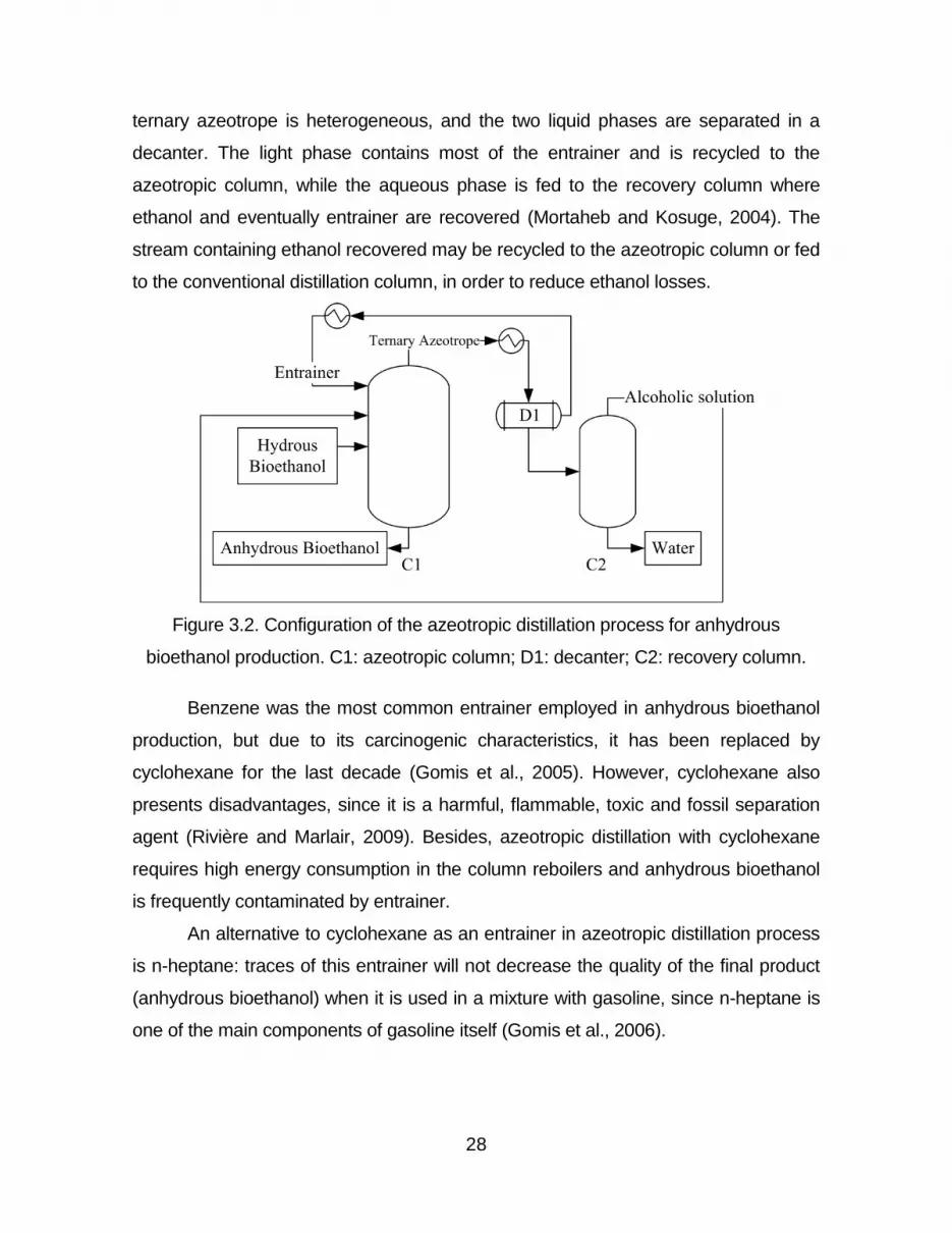
28

ternary azeotrope is heterogeneous, and the two liquid phases are separated in a

decanter. The light phase contains most of the entrainer and is recycled to the

azeotropic column, while the aqueous phase is fed to the recovery column where

ethanol and eventually entrainer are recovered (Mortaheb and Kosuge, 2004). The

stream containing ethanol recovered may be recycled to the azeotropic column or fed

to the conventional distillation column, in order to reduce ethanol losses.

Figure 3.2. Configuration of the azeotropic distillation process for anhydrous

bioethanol production. C1: azeotropic column; D1: decanter; C2: recovery column.

Benzene was the most common entrainer employed in anhydrous bioethanol

production, but due to its carcinogenic characteristics, it has been replaced by

cyclohexane for the last decade (Gomis et al., 2005). However, cyclohexane also

presents disadvantages, since it is a harmful, flammable, toxic and fossil separation

agent (Rivière and Marlair, 2009). Besides, azeotropic distillation with cyclohexane

requires high energy consumption in the column reboilers and anhydrous bioethanol

is frequently contaminated by entrainer.

An alternative to cyclohexane as an entrainer in azeotropic distillation process

is n-heptane: traces of this entrainer will not decrease the quality of the final product

(anhydrous bioethanol) when it is used in a mixture with gasoline, since n-heptane is

one of the main components of gasoline itself (Gomis et al., 2006).

29

Extractive Distillation

In extractive distillation, also known as homogeneous azeotropic distillation, a

separating agent, called solvent or entrainer, is added to the azeotropic mixture in

order to alter the relative volatility of the components in the original mixture.

In the conventional extractive distillation process, solvent is fed to the first

column (extractive column), above the azeotropic feed. Anhydrous ethanol is

produced on the top of the extractive column, while in the bottom a mixture containing

solvent and water is obtained. The solvent is recovered in a second column (recovery

column), cooled and recycled to the extractive column (Huang et al., 2008).

An alternative configuration for this process makes use of a single column. On

its top, anhydrous ethanol is produced, while pure solvent is recovered on the bottom.

By means of a side draw of water in vapour phase located a few stages above the

bottom, pure water is obtained (Brito et al., 1997). Configuration of conventional and

alternative extractive distillation process is depicted in Fig. 3.3.

Meirelles et al. (1992) demonstrated that monoethyleneglycol (MEG) is an

efficient solvent for anhydrous bioethanol production by extractive distillation. This

process was first employed in industrial scale in Brazil in the 2001 sugarcane harvest

season, and is today one of the most common processes along with azeotropic

distillation with cyclohexane and adsorption onto molecular sieves.

Figure 3.3. Configuration of conventional (a) and alternative (b) extractive distillation

process for anhydrous bioethanol production. C1: extractive column; C2: recovery

column.

30

The solvent most used in industry for the separation of ethanol - water

mixtures is MEG, which is fossil and toxic. The use of bioglycerol – by-product of

biodiesel production – as a substitute of MEG has been encouraged due to its

availability and low price. Besides, bioglycerol is not harmful to humans or the

environment, thus can be safely used to produce anhydrous ethanol for use in food or

pharmaceutical industries (Dias et al., 2008).

Novel separating agents for the extractive distillation process, ionic liquids (IL)

and hyperbranched polymers (HyPol) have been studied for the past few years with

great interest (Huang et al., 2008; García-Miaja et al., 2008; Pereiro and Rodríguez,

2008; Seiler et al., 2004).

Ionic liquids (IL), usually a mixture of organic cation and inorganic anion,

possess several characteristics that make them suitable agents for the separation

of the ethanol-water azeotrope in extractive distillation processes, such as low

viscosity, thermal stability, good solubility and low corrosiveness (Huang et al.,

2008). Since those properties can be customized, IL appear superior to many

conventional entrainers and extractive solvents (Seiler et al., 2004).

Hyperbranched polymers (HyPol) are highly branched macromolecules with a

large number of functional groups. Their properties, such as remarkable selectivity

and capacity, low viscosity and thermal stability, make them suitable agents for

extractive distillation process (Huang et al., 2008). Since their polarity can be

adjusted by their functional end groups, suitable solvents can be designed for specific

operations (Seiler et al., 2004).

Some of the advantages of the IL and HyPol reside on the fact that they do not

contaminate the final product (anhydrous bioethanol), since they are not volatile, and

because the entrainer recovery process does not require distillation columns (Huang

et al., 2008), a stripping column working with air may be used to promote entrainer

regeneration, as depicted in Figure 3.4.

31

Figure 3.4: Example of extractive distillation process configuration with non-volatile

entrainers Ionic Liquid (IL) or low-viscosity Hyperbranched Polymers (HyPol); C1:

main column, C2: flash, C3: stripping column (adapted from Seiler, 2006).

Adsorption

Adsorption involves the transfer and resulting equilibrium distribution of one

or more solutes between a fluid phase and particles (Perry et al., 1997). Usually,

inorganic adsorbents are employed, such as molecular sieves, lithium chloride,

silica gel and activated alumina. Besides, Huang et al. (2008) also report the use of

bio-based adsorbents, such as cornmeal, cracked corn, starch, corn cobs, wheat

straw, bagasse, cellulose, hemicellulose, wood chips and other grains, which are

biodegradable and derived from renewable resources (Al-Asheh et al., 2004).

In the ethanol dehydration process by adsorption onto molecular sieves, a

fixed bed packed with zeolites is employed in order to adsorb water present in

hydrous ethanol, producing anhydrous ethanol. 3A zeolite molecular sieves are

generally used in this process, which corresponds to a nominal pore size of 3

Angstroms (0.30 nm). In view of their small diameter (0.28 nm), the water molecules

can easily penetrate the structural zeolite canals, while most of the ethanol molecules

(0.44 nm) are simultaneously excluded (Carmo and Gubulin, 2002).

Brazilian biorefineries configuration of the dehydration process by adsorption

includes three adsorbent beds in a cyclic operation: one of them is regenerating

(water accumulated in adsorbent is removed) while in the others adsorption is carried

out. Hydrous ethanol on vapour phase (about 93 wt%) is fed to the molecular sieves

32

bed. A vacuum pump is used to promote regeneration of the bed and the aqueous

solution recovered is recycled to the distillation stage, since it contains a large

amount of ethanol. The configuration of the adsorption process for anhydrous

bioethanol production used in Brazil is depicted in Figure 3.5.

Figure 3.5. Configuration of the adsorption onto molecular sieves process for

anhydrous bioethanol production. HE1: superheater; HE2, HE3: condensers; MS1:

regenerating molecular sieves bed; MS2, MS3: molecular sieves beds.

Adsorption using molecular sieves allows the production of high purity ethanol

without contamination by solvent; besides, it requires less energy when compared to

distillation-based processes, given that only one vaporization step is necessary.

However, a barrier to its use by Brazilian biorefineries is the high investment cost,

since zeolites are not produced in Brazil; this problem may be completely surpassed

when bio-based adsorbents become viable.

One of the most important characteristics of the configuration of the adsorption

process employed in Brazil is that hydrous ethanol is produced in the distillation

columns as a liquid and fed to the molecular sieves beds as a superheated vapour,

thus energy is required to promote its vaporization; because hydrous ethanol must

be fed to the beds at around 3 bar, it is easier to raise the pressure of the liquid phase

ethanol and then to vaporize it, instead of compressing hydrous ethanol vapours

obtained directly from the distillation columns. As a result, there is an increase on the

steam consumption of the process. Another disadvantage is the high vacuum

33

required to bed regeneration due to the strong zeolites-water interaction (Huang et

al., 2008).

Electromagnetic as well as mechanical waves have been studied as

regeneration methods for loaded adsorbents; Reuβ et al. (2002) has studied the use

of microwaves to enhance desorption, which strongly depends on the

electromagnetic properties of adsorbent and solvents adsorbed. Their work included

experiments with ethanol/acetone, ethanol/toluene and ethanol/water systems and

their results showed that polar components, such as ethanol and water, present

enhanced desorption.

Pervaporation

Pervaporation is a membrane process in which a phase change from liquid to

vapour occurs. In this process, the feed mixture is a liquid and one component in the

mixture permeate preferentially through the membrane and evaporate as a result of

the partial pressure on the permeate side being held lower than the saturation vapour

pressure. The driving force is controlled by applying a vacuum or occasionally with a

sweep gas on the permeate side. Pervaporation membranes are chosen for high

selectivity, and the permeate is often highly purified (Perry et al., 1997; Coulson et al.,

2002). Configuration of the pervaporation process for anhydrous bioethanol

production is represented in Figure 3.6.

Figure 3.6. Configuration of the pervaporation process for anhydrous bioethanol

production.

34

It is possible to use the pervaporation system to concentrate the mixture

obtained after fermentation, which is a dilute ethanol solution, as well as to

concentrate hydrous ethanol obtained after distillation of the fermentation broth.

Nevertheless, fermentation broth components may impact pervaporation membranes

and modules. Vane (2005) reports several works available in the literature which

evaluate the impacts of broth components on membranes, such as suspended solids

and yeast cells, which may potentially accumulate in modules, blocking flow path and

membrane surface, and glucose, which decreases water and ethanol fluxes. These

problems would be diminished in the case where pervaporation is employed only as a

method for ethanol dehydration, since those undesired broth components are

removed in the vinasse.

In order to reduce the fouling potential of solids in the fermentor broth, a pre-

pervaporation solid–liquid separation device may be employed, thus allowing the use

of the full range of pervaporation module options. In fact, the simplest situation would

be one in which the pervaporation modules are able to accept the fermentation broth

as delivered from the fermentor (including solids) and the broth contains no

temperature-sensitive components or they are no longer necessary in the process.

However, the addition of any separation device to the system adds capital and

operating costs (Vane, 2005).

Ultrasonic Separation

Ultrasonic separation consists of the fragmentation of a liquid layer to form a

fine droplet mist by high frequency ultrasonic atomization and it has been applied to a

range of industrial applications such as fine chemical manufacturing, pharmaceutical

production, and food processing (Suzuki et al., 2006).

In this context, Sato et al. (2001) have shown that pure ethanol can be

obtained through ultrasonic atomization of ethanol-water solutions with several

concentrations at relatively low temperature (10 ºC). Since the enrichment ratio

provided by this technique is much higher than that expected for the vapour in

equilibrium with the original mixture and the required energy is much smaller than that

required for liquid vaporization, ultrasonic separation has the potential to become an

alternative to distillation (Yano et al., 2007).

35

Suzuki et al. (2006) conducted experiments in batch and continuous feed

processing systems and observed that ethanol concentration of the mist and the

ethanol collection rate were significantly increased and maintained constant in the

continuous feed system, which is explained by the low variation in the ethanol feed

concentration and constant liquid level in the separation vessel.

HYBRID PROCESSES

Hybrid separation processes combine two or more of the techniques described

above, as well as fermentation processes, in order to create optimized processes and

increase their efficiency.

Pervaporation/vapour permeation coupled with distillation

One of the most promising approaches consist of integrated pervaporation and

distillation systems (Szitkai et al., 2002), on which the pervaporation module may be

located at the final stage of dehydration, to produce anhydrous bioethanol, or

immediately after the fermentation process, substituting the distillation and

rectification columns in order to produce hydrous bioethanol, or part of a hybrid

system using other dehydration methods (29).

For the ethanol – water system, Pressly and Ng (1998) evaluated the

influence of different feed concentrations in the costs and observed that the lowest

concentration studied (0.1 mol fraction ethanol) presented the highest scaled

break-even cost overall. Therefore, the configuration that employs pervaporation

after distillation is more economically attractive, since its pervaporation module is

fed with a mixture of high concentration.

Szitkai et al. (2002) describe a system with a distillation column, which

purifies the crude ethanol inlet, and a succeeding network of pervaporation

membrane modules. The top product of the column is fed to the first section of the

membrane train. In each membrane section the retentate is collected and fed to a

heat exchanger for re-heating. There is a vacuum pump at the permeate side of

the membrane system. The permeate is withdrawn as a product stream and/or

recycled to the column feed. Results showed that total permeate recycling is more

economical, when compared to partial recycling.

36

Pervaporation coupling with distillation is a potential alternative, since

pervaporation alone will rarely be economical due to the purity required nowadays

in production and the limitation on flux given by the activity as the driving force of

the pervaporation process (Lipnizki et al., 1999).

Another similar option is to feed hydrous ethanol vapours obtained in

conventional distillation directly to a vapour permeation membrane system (Sato et

al., 2008), what does not require the total condensation of the rectification column

top product (hydrous bioethanol), thus decreasing water consumption in the

bioethanol production process. Sato et al. (2008) successfully produced anhydrous

bioethanol (over 99.6 wt%) with NaA zeolite membranes, by coupling conventional

distillation, where hydrous bioethanol (88 wt% ethanol) is produced, and two

membrane modules for vapour permeation.

Coupled Fermentation/Pervaporation

Accumulation of ethanol in the fermentation broths can lead to a decrease in

ethanol productivity due to low activity of the biocatalyst, which is known as product

inhibition. Therefore, the removal of ethanol from the fermentation reactor is

indispensable and a possible solution is the pervaporation with ethanol-selective

hydrophobic membranes, which allows ethanol to be continuously removed from the

fermentation system and simultaneously concentrated (Ikegami et al., 1997).

O’Brien and Craig (1996) studied a conventional yeast fermentation coupled to

a flat-plate membrane pervaporation unit using a commercially available

polydimethylsiloxane membrane. A concentrated dextrose was fed to the system

and, as a result, an enriched ethanol stream (20-23 wt% ethanol) was continuously

recovered from the fermentation broth and a level of 4-6 wt% ethanol was maintained

in the fermentation reactor.

Ikegami et al. (1997) also investigated the performance of a coupled

fermentation/pervaporation process, but using silicalite membranes. They observed a

20 % increase in an average glucose consumption rate as compared with that without

the pervaporation unit. In addition, ethanol concentrations in the permeate reached

85 % (v/v).

37

Liquid-Liquid Extraction-Fermentation Hybrid

Liquid–liquid extraction combined with fermentation is also employed to

remove ethanol and other inhibitory compounds, causing an increase in the

ethanol yield (Huang et al., 2008).

Minier and Goma (1981) proposed the coupling of plug flow reactor and

liquid-liquid extraction with n-dodecanol as a solvent. Alcoholic fermentations on

glucose syrup at 35 °C using Saccharomyces cerevisiae was carried out and the

results showed that ethanol productivity was multiplied by 5 and a solution of 407

g/L of glucose, considered a highly concentrated feed, was totally fermented.

Gyamerah and Glover (1996) constructed a continuous pilot plant for

fermentation production of ethanol, using liquid-liquid extraction to remove the

product and with recycle of the fermented broth raffinate. The plant was fed with

glucose concentrations in the range 10.0-45.8 wt%, n-dodecanol – used as a

solvent – and immobilised yeast to overcome the problem of emulsification. It was

observed that for a feed glucose concentration of 45.8 wt%, the aqueous purge

was equivalent to 2.8 m³ of effluent per m³ of ethanol produced and represented a

78 % reduction in the volume of the aqueous purge compared with using a feed

containing 10 wt% glucose.

Continuous fermentation coupled with vacuum flash chamber

Silva et al. (1999) studied the technical viability and the dynamic response of

the continuous extractive alcoholic fermentation, which consists of a fermentation

reactor coupled with an extractive vacuum flash chamber. Results showed that the

temperature could be maintained at desirable levels without using heat exchangers

for the temperature control, besides the partial removal of ethanol increased

significantly the productivity.

In this context, experiments conducted by Atala (2004) using

Saccharomyces cerevisiae and concentrated sugarcane molasses, containing up

to 330 g/l of sugar, showed that an alcoholic solution of 50 °GL can be obtained.

Furthermore, the fermentation reactor operated with concentrations of ethanol at 5

°GL, which is a weakly inhibitory value for the yeast of the process.

38

CONCLUSION

Novel separations processes have been proposed for ethanol purification and

dehydration in order to substitute or assist distillation-based processes.

In order to replace azeotropic and extractive distillation, the most used process

for ethanol dehydration in Brazilian biorefineries, adsorption, pervaporation and

ultrasonic separation seem to be better alternatives regarding energy consumption

and use of eco-friendly separation agents, along with the substitution of fossil-derived

solvents in azeotropic and extractive distillation by renewable or less pollutant ones.

Besides, hybrid process such as pervaporation/distillation and integrated

fermentation and separation processes may improve the efficiency of the bioethanol

production process: by coupling different processes, each process may be employed

on its optimum conditions, thus combining their individual advantages.

However, the use of these new processes or solvents faces many barriers in

Brazil. One of them is the fact that the Brazilian bioethanol industry is very

traditionalist, and new technologies usually take longer to be employed in bioethanol

production than in other sectors of the industry. The high capital cost of these new

technologies is also an obstacle to the replacement of old processes, especially

because several equipments and separating agents are produced abroad.

Improvements on the fermentation step may also improve bioethanol

production sustainability when regarding the purification step. Integrated fermentation

and separation process, like extractive fermentative processes, allow the continuous

removal of ethanol from the fermentor, in order to prevent product inhibition on yeast

cells, thus a more concentrated substrate can be supplied to fermentation reactor.

Therefore, a wine of higher ethanol concentration can be obtained and, consequently,

volumes of residue generated are diminished, as well as energy consumption in the

purification step.

It is of fundamental importance to decrease both energy consumption and

residue generation on the bioethanol production process. Integration of different

fermentation and separation processes, thermal integration of distillation columns,

use of less energy-intensive dehydration systems and of more efficient separating

agents, as described in this work, are essential to achieve those goals.

39

3.3. Comentários e Conclusões

Neste capítulo, foram apresentados os processos usuais de separação para

a concentração e desidratação do etanol bem como novos processos que possam

auxiliar ou substituir processos baseados na destilação.

A avaliação das alternativas indicou que os processos de adsorção,

pervaporação e separação ultrassônica são alternativas atraentes para a

desidratação do etanol bem como a utilização de agentes de separação

ambientalmente amigáveis na destilação extrativa.

Além disso, o uso de processos híbridos como pervaporação/destilação e

da fermentação integrada a outros processos de separação podem aumentar a

eficiência do processo de separação, uma vez que a combinação dos processos

permite utilizar cada um destes em suas condições ótimas.

Por fim, apresenta-se, através da Tabela 3.1, um resumo das aplicações,

vantagens e desvantagens de cada processo apresentado na seção 3.2.

40

Tabela 3.1. Comparação entre os processos apresentados.

Processo Aplicação Vantagem Desvantagem

Destilação múltiplo efeito

Concentração Redução no consumo de

energia/ Menor quantidade de trocadores de calor

Uso de diferentes níveis de pressão pode requerer o

emprego de compressores

Destilação Azeotrópica

com Cicloexano

Desidratação Uso da infra-estrutura já

existente nas usinas

Uso de agente de separação fóssil e tóxico / Alto consumo

energético / Processo de operação complexa

Destilação Azeotrópica

com n-Heptano

Desidratação

Pode aproveitar infra-estrutura existente nas usinas /

Contaminação por solvente não afeta a qualidade do produto a

ser adicionado à gasolina

Uso de agente de separação fóssil e tóxico / Alto consumo

energético / Processo de operação complexa

Destilação Extrativa com

MEG Desidratação

Menor consumo de energia comparada à destilação

azeotrópica

Uso de agente de separação fóssil e tóxico


Glicerol Desidratação

Menor consumo de energia comparado à destilação

azeotrópica / Baixo custo do solvente / Solvente não-tóxico e

de origem renovável

Decomposição do glicerol (altas temperaturas) gera

substância tóxica


IL/HyPol Desidratação

Menor consumo de energia / Os solventes podem ser

customizados para a separação desejada / Baixa volatilidade permite recuperação sem uso

de destilação

IL que possui ânion halogenado é caro e

apresenta baixa estabilidade, pode formar substância

tóxica e corrosiva

Adsorção em peneiras

moleculares Desidratação

Não apresenta contaminação por solvente / Necessita menos energia do que os processos de

destilação

Necessidade de regeneração do leito / Reciclo de solução

alcoólica à etapa de concentração / Alto custo das

zeólitas (importação)

Pervaporação Concentração / desidratação

Menor consumo de energia Presença de sólidos no vinho pode inviabilizar a etapa de

concentração / Fluxo limitado

Separação Ultrassônica

Concentração/ desidratação

Menor consumo de energia -

Pervaporação/ Destilação

Concentração/ desidratação

Menor consumo de energia comparado à destilação / O acoplamento pode permitir

utilizar ambos os processos em suas condições ótimas

-

Fermentação/ Pervaporação

Fermentação/ concentração

Aumento da taxa de reação / Produção de vinho mais

concentrado

Presença de sólidos no vinho pode inviabilizar a etapa de

concentração Fermentação/

Extração líquido-líquido


Aumento da taxa de reação / Produção de vinho mais

concentrado -

Fermentação extrativa a

vácuo


Produção de vinho mais concentrado / Dispensa o uso

de trocador de calor na fermentação

-

41

Capítulo 4

Caracterização Termodinâmica

4.1. Introdução

No processo de produção de bioetanol, há uma grande variedade de

componentes devido à formação de subprodutos e à ocorrência de reações

paralelas na etapa de fermentação. Condições do processo fermentativo, tais

como temperatura, pH e concentração de açúcares, influenciam significativamente

a composição do vinho produzido. A qualidade da matéria-prima e do fermento

utilizados, teor alcoólico do meio, aditivos químicos, tipo do processo fermentativo

(batelada ou contínuo) também podem afetar o comportamento da levedura e,

consequentemente, induzir à formação de outros compostos.

Portanto, além de etanol e água, podem ser encontrados açúcares, outros

alcoóis, ácidos orgânicos, acetaldeído, acetona e glicerol. Considerando-se a

produção de bioetanol de 2ª geração, tem-se que a hidrólise do bagaço de cana-

de-açúcar pode também gerar furfural, 5-hidroxi-metil-furfural (HMF) e pentose.

Com relação ao processo de desidratação do etanol, a destilação

azeotrópica com cicloexano e a destilação extrativa com monoetilenoglicol

também são baseadas no equilíbrio de fases, sendo importante também a

consideração destes componentes na caracterização do sistema.

A caracterização do sistema é essencial para entender o comportamento

dos componentes nas colunas de destilação, portanto a utilização de modelos

termodinâmicos apropriados para representar o sistema é de grande importância

na simulação de processos.

Com o intuito de avaliar a acurácia dos modelos termodinâmicos presentes

no banco de dados do simulador Aspen Plus®, foram pesquisados na literatura

dados experimentais de equilíbrio para os binários presentes no sistema. Em

seguida, estes dados foram comparados com os resultados fornecidos pelo

simulador utilizando os modelos de coeficientes de atividade UNIQUAC (Universal

Quasi-Chemical) e NRTL (Non-Random Two Liquid).

42

Realizou-se também a análise de diagramas T-x-y e y-x a fim de observar a

ocorrência de não-idealidades, como azeotropia, miscibilidade parcial e baixa e

alta volatilidade relativa.

Na Tabela 4.1 são apresentados os componentes considerados na análise

dos modelos termodinâmicos bem como as respectivas temperaturas de ebulição

estimadas pelo simulador Aspen Plus®.

Tabela 4.1. Temperaturas de ebulição dos componentes envolvidos no processo

de produção de bioetanol a pressão atmosférica.

Componente Temperatura de ebulição (ºC)

Acetaldeído 21,1

Acetona 56,1

Metanol 64,5

Acetato de Etila 77,2

Etanol 78,3

Cicloexano 80,8

n-Propanol 97,2

Água 100,0

Isobutanol 107,7

n-Butanol 117,7

Ácido Acético 118,0

Álcool Isoamílico 130,9

Furfural 161,4

Monoetilenoglicol 197,1

Glicerol 287,7

Glicose 343,8

Sacarose 477,7


intitulado “Phase equilibrium data for binary mixtures in bioethanol production -

evaluation of thermodynamic models adequacy” a ser submetido a periódico

internacional.

43

4.2. Phase equilibrium data for binary mixtures in bioethanol

production - evaluation of thermodynamic models adequacy

ABSTRACT

One of the most important tools used to evaluate new technologies and alternative

processes is the process simulation software. In order to appropriately represent

the thermodynamic properties of a system, thermodynamic models employed must

be consistent with experimental phase equilibrium data.

In bioethanol production, a large number of components are found due to the

complexity of the raw material and to the generation of a number of products

during fermentation reactions, thus increasing complexity of the thermodynamic

representation of the bioethanol production process. The purification step is mainly

based on distillation process, and as such it is strongly dependent on vapor-liquid

or vapor-liquid-liquid equilibrium.

In this work a phase equilibrium study of components found in bioethanol

production was carried out using results predicted by Aspen Plus® and

experimental data available in the literature. Several deviations from ideal

behaviour were observed for many binary systems.

INTRODUCTION

Improvements on bioethanol production process have been increasingly

investigated, mainly due to climate change and predicted depletion of fossil

resources. One of the most important tools used to study process alternatives and

to evaluate their impacts on process yields, energy consumption and costs is the

process simulation software. Nevertheless, the simulation must employ the

appropriate thermodynamic models to properly predict process behavior (Cardona

and Sánchez, 2007). The thermodynamic models provided in the databanks also

determine the efficiency of simulation packages (Abderafi and Bounahmidi, 1994).

The reliable knowledge of the thermophysical properties of the pure

compounds and their binary and higher mixtures is essential for the design and

optimization of chemical processes. Considering specially the separation

processes, the reliable knowledge of the phase equilibrium behaviour of the

44

systems considered is of special importance (Gmehling, 2009).

A large number of components are found in the bioethanol production

process due to fermentation by-products and parallel reactions. Process

fermentation conditions, such as temperature, pH and sugars concentration,

significantly influence the composition of the wine produced. Ethanol and water are

the main components found in wine; however, methanol, propanol, isobutanol,

isoamyl alcohol, acetaldehyde, acetone, acetic and succinic acids, ethyl acetate,

glycerol, glucose and sucrose are also present in low concentrations. Considering

the production of 2nd generation bioethanol, furfural, 5-hydroxymethyl-furfural and

pentose might be present as well, depending on the chosen hydrolysis process.

In addition, in the purification process, extractive distillation with

monoethyleneglycol as solvent and azeotropic distillation with cyclohexane as

entrainer can be employed in order to obtain anhydrous bioethanol. These

operations are based on the phase equilibrium, so a previous detailed study about

these component interactions is necessary to understand columns behaviour and

to predict more accurate results.

For instance, Faúndez and Valderrama (2004) analyzed binaries of ethanol

and water with congeners through calculation of deviations between predicted and

experimental temperatures and vapor mole fractions. NRTL model, PSRK equation

of state and UNIFAC method were considered in this evaluation and it was

observed that NRTL model suitably represents the system. However, sugars and

entrainers employed in ethanol dehydration were not taken into account in their

work.

In this work, a phase equilibrium study was carried out using results

predicted by Aspen Plus® and experimental data available in the literature. Non-

Random Two-Liquid (NRTL) and Universal Quasi-Chemical (UNIQUAC)

thermodynamic models for calculation of the activity coefficient on the liquid phase

were employed and compared to experimental data, in order to evaluate if they

represent the system behaviours appropriately. Furthermore, non-ideal behaviours

were evaluated in order to understand the interaction between components in the

mixture.

45

DATA AVAILABLE IN THE LITERATURE

The first step to evaluate the relevant data consisted on selecting the most

important components present on bioethanol production. Those include besides

water and ethanol, sugarcane components, such as glucose and sucrose, by-

products generated during fermentation reactions, such as other alcohols, organic

acids, acetaldehyde, acetone, and glycerol, as well as components that may be

generated on 2nd generation bioethanol production, like furfural, 5-hydroxymethyl-

furfural (HMF) and pentose.

Secondly, an extensive research was carried out to determine which

binaries are available in the literature. The first sources consulted were the

DECHEMA equilibrium data collections (Gmehling et al., 1982a-c; Gmehling et al.,

1981; Gmehling, 1993); data for binary pairs not available in those sources were

searched for in journals. Data for most of the pairs containing water or ethanol was

obtained. On Table 4.2 the references for each binary pair is depicted.

Table 4.2. Sources for the binary pairs equilibrium data.

Component 1 2 3 4 5 6 7 8 9 10 11 12 13 14 15

1- Ethanol

2- Water 2,10

3- Methanol 2,10 10

4- Propanol 4 3

5- Isobutanol 2 4 3

6- n-Butanol 4 3 3

7-Isoamyl alcohol 2,16 3

8- Acetaldehyde 12 12,4 3 3

9-Acetone 8,6 15 6

10- Acetic acid 2 4 17 11 6

11- Ethyl acetate 2 5 5 16 18

12- Glycerol 7 4,7,9 7 7 7

13- Glucose 1

14- Sucrose 1

15- Furfural 13 6 6 14 6

[1] Abderafi & Bounahmidi (1994)

[2] Gmehling et al. (1982a)

[3] Gmehling et al. (1982b)

[4] Gmehling et al. (1981)

[5] Gmehling et al. (1982c)

[6] Gmehling (1993)

[7] Oliveira et al. (2009)

[8] Lee & Hu (1995)

[9] Chen & Thompson (1970)

[10] Christensen (1998)

[11] Lee et al. (2000)

[12] d’Avila & Silva (1970)

[13] Wisniak & Polishuk (1999)

[14] Fele & Grilc (2003)

[15] Tu et al. (1997)

[16] Sanz & Gmehling (2008)

[17] Arlt (1999)

[18] Kato (1988)

46

The next step consisted of plotting experimental data along with that

predicted using NRTL and UNIQUAC models with the Aspen Plus® process

simulator. A large number of plots was generated, for instance, a T-x-y diagram for

the ethanol – water system is shown on Figure 4.1 to provide an example of what

was done for all the binaries cited in Table 4.2.

Figure 4.1. T-x-y diagram for the ethanol (1) - water (2) system, at 760 mm Hg.

Thus, it is possible to evaluate if the two models employed for calculation of

the activity coefficient on the liquid phase (NRTL and UNIQUAC) are in agreement

with experimental data. In the case of ethanol and water, both models represent

appropriately the system behavior, including the azeotrope.

Most of the systems were suitably represented by both NRTL and

UNIQUAC models, with a few systems being represented better by NRTL and

some by none. Table 4.3 summarizes the results of the comparison between

experimental data and the thermodynamic models, indicating the model that better

represents each binary.

0.0 0.1 0.2 0.3 0.4 0.5 0.6 0.7 0.8 0.9 1.076

78

80

82

84

86

88

90

92

94

96

98

100

102

T (

°C)

x1, y

1

Experimental

UNIQUAC

NRTL

47

Table 4.3. Representative model for each binary.

Component 1 2 3 4 5 6 7 8 9 10 11

1- Ethanol

2- Water Both

3- Methanol Both Both

4- Propanol Both Both

5- Isobutanol Both Both Both

6- n-Butanol Both Both Both

7-Isoamyl alcohol Both Both

8- Acetaldehyde Both Both Both Both

9-Acetone Both Both Both

10- Acetic acid Both Both Both NRTL Both

11-Ethyl acetate Both Both Both Both Both

12- Glycerol Both None Both Both Both

13- Glucose None

14- Sucrose None

15- Furfural Both Both Both NRTL Both

Binary interaction parameters available in the process simulator were

checked, since a collection of built-in binary parameters for the activity coefficient

models (NRTL and UNIQUAC) are available in Aspen Plus® database, as well as

some equation-of-state (EOS) models and Henry's law, different databank

parameters are available (Aspen Plus Help, 2000). For instance, these comprise

VLE-IG (NRTL and UNIQUAC models with ideal gas vapor EOS), VLE-HOC

(Wilson, NRTL and UNIQUAC models with Hayden-O'Connell vapor EOS), VLE-

LIT (NRTL and UNIQUAC models with ideal gas vapor EOS, obtained from the

literature). Even though on the majority of the cases the appropriate databank is

automatically chosen, in some situations parameters retrieved from VLE-HOC

represented the process behavior more accurately. This was the case in the

parameters containing acetic acid, as an example.

The most significant deviation of the experimental data was verified in the

binary pairs containing water and sugar (sucrose and glucose), for which both

NRTL and UNIQUAC models predicted the boiling point temperature in accordance

with experimental data (Abderafi and Bounahmidi, 1994) only for solutions with low

sugar content (less than 10 %). However, different works predicting binary or

48

thermodynamic data for sugar systems are available in the literature (Abderafi and

Bounahmidi, 1999; Peres and Macedo, 1997) using UNIFAC or other property

methods. For example, T-x diagram for the binary water-sucrose is shown in

Figure 4.2. From this figure, it is observed that UNIQUAC provided a slightly better

prediction, since its curve coincides with experimental data until 20 % (mole basis).

Figure 4.2. T-x diagram for the sucrose (1) - water (2) system, at 760 mm Hg.

In addition, for the pairs acetic acid – furfural or isoamyl alcohol, only the

NRTL model (with VLE-HOC parameters) suitably represented experimental data.

For instance, T-x-y diagram for acetic acid – furfural is depicted in Figure 4.3. In

this case, prediction of the system behavior given by UNIQUAC model was

erroneous, since it forecasted an azeotrope between acetic acid and furfural that

does not exist in practice as shown by experimental data (Fele and Grilc, 2003).

0.0 0.1 0.2 0.3 0.4 0.5 0.6 0.7 0.8 0.9 1.090

100

110

120

130

140

150

160

170

180

190

T (

°C)

x1

Experimental

NRTL

UNIQUAC

49

Figure 4.3. T-x-y diagram for the acetic acid (1) - furfural (2) system, at 667 mmHg.

For water-glycerol system, NRTL and UNIQUAC provided a correct

representation only for the liquid phase as can be seen in Figure 4.4.

Figure 4.4. T-x-y diagram for the water (1) - glycerol (2) system, at 760 mm Hg.

In spite of the mentioned divergences, NRTL equation yields the best overall

results for the binary mixtures investigated in this work. However, UNIQUAC also

provides satisfactory predictions for the main binaries present in the mixture.

0.0 0.1 0.2 0.3 0.4 0.5 0.6 0.7 0.8 0.9 1.0110

115

120

125

130

135

140

145

150

155

160

T (

°C)

x1, y

1

Experimental

NRTL

UNIQUAC

0.0 0.1 0.2 0.3 0.4 0.5 0.6 0.7 0.8 0.9 1.0 1.180

100

120

140

160

180

200

220

240

260

280

300

T (

°C)

x1, y

1

Experimental

UNIQUAC

NRTL

50

Regarding system behavior, several deviations from ideality were verified,

such as low and high relative volatility, azeotropes and the formation of two liquid

phases. These characteristics are assembled in Table 4.4.

Table 4.4. Behavior of selected binary pairs.

Behavior Binary Pairs

Azeotrope

Ethanol - Water Ethyl acetate

- Water Water -

Propanol n-Butanol -

Water Isobutanol -

Water

Isoamyl alcohol - Acetic acid

Acetone - Methanol

Water - Furfural

Ethyl acetate - Ethanol

Two liquid phases

Water – Propanol

n-Butanol -Water

Isobutanol - Water

Ethyl acetate - Water

Water - Furfural

Low relative volatility

Ethanol - Methanol

Acetone - Ethanol Acetone- Methanol

Ethyl acetate - Ethanol

Isobutanol – Butanol

Isobutanol – Isoamyl alcohol

Acetic acid - Isoamyl alcohol

Ethanol - Isobutanol

Acetaldehyde – Acetone

Ethanol - Acetic acid

Acetic acid - Water

Acetic acid - furfural

High relative volatility

Glycerol - Ethanol Glycerol - Water Glycerol - Methanol

Glycerol - Propanol

n-Butanol - Acetaldehyde

Furfural - Ethanol Water -

Acetaldehyde

DATA NOT AVAILABLE IN THE LITERATURE

Vapor-liquid equilibrium (VLE) data was not found in the literature for several

pairs encountered among the components studied in this work. For some reactive

systems, such as those present in alcohol – acid systems, experimental data are

found only for low temperatures, on which esterification reactions are very slow

(Arlt, 1999), thus special equipment is needed to acquire VLE data. Arlt (1999)

developed an apparatus to acquire data for such systems (e.g., methanol – acetic

acid), but only data for the liquid phase was obtained due to problems in

determining vapor phase composition. For several pairs, only experimental data for

the liquid phase and either the boiling temperature or vapor phase composition

were obtained and, in these situations, the data available was plotted and

compared in different diagrams, such as x-y diagrams. This was the case for some

of the glycerol-containing pairs, for instance.

51

Data for binary pairs containing either HMF (5-hydroxymethyl-furfural) or

pentose were not found in the literature. HMF is an important by-product of

cellulose hydrolysis derived from glucose decomposition, but it is not available on

the process simulator database. It would be important to gather that data and to

make this component available in the database of Aspen Plus®.

Data for binary pairs involving succinic acid were not found as well. Even

though its concentration remains at low levels during bioethanol production

process, succinic acid is a very important carboxylic acid produced during alcoholic

fermentation. Thus, experimental equilibrium data for this component is important

as well.

DEHYDRATION COMPONENTS

A separate study was carried out to verify equilibrium data for components

present on the dehydration operations. The most frequently employed distillation-

based separation processes (extractive distillation with monoethyleneglycol, MEG,

and azeotropic distillation with cyclohexane) were considered. Since those

processes use hydrous ethanol produced on the distillation columns, only ethanol,

water and entrainer (monoethyleneglycol and cyclohexane) are considered.

Since a heterogeneous azeotrope is formed between water, ethanol and

cyclohexane, a ternary diagram for the liquid-liquid equilibrium between those

components was made (Gomis et al., 2005), besides the individual binary pair for

VLE data. It was verified that both models represent the ternary liquid-liquid

equilibrium of the system appropriately; the ternary diagram is depicted in Figure

4.5.

52

Figure 4.5. Ternary diagram for the ethanol – water - cyclohexane system, at 760

mmHg and 35 ºC.

Data for the binary system ethanol – MEG (Gmehling et al., 1982a) and water –

MEG (Gmehling et al., 1981) are illustrated in Figures 4.6 and 4.7. NRTL and

UNIQUAC provided the same predictions and appropriately represented the

system, except for liquid phase in the T-x-y diagram for binary water – MEG.

Figure 4.6. T-x-y diagram for the water (1) – MEG (2) system, at 760 mmHg.

0.00 0.25 0.50 0.75 1.00

0.00

0.25

0.50

0.75

1.00 0.0

0.2

0.4

0.6

0.8

1.0 Experimental

NRTL

UNIQUAC

Cyc

loeh

exan

e

Ethanol

Water

0.0 0.1 0.2 0.3 0.4 0.5 0.6 0.7 0.8 0.9 1.0 1.190

100

110

120

130

140

150

160

170

180

190

200

210

T (

°C)

x1, y

1

Experimental

UNIQUAC

NRTL

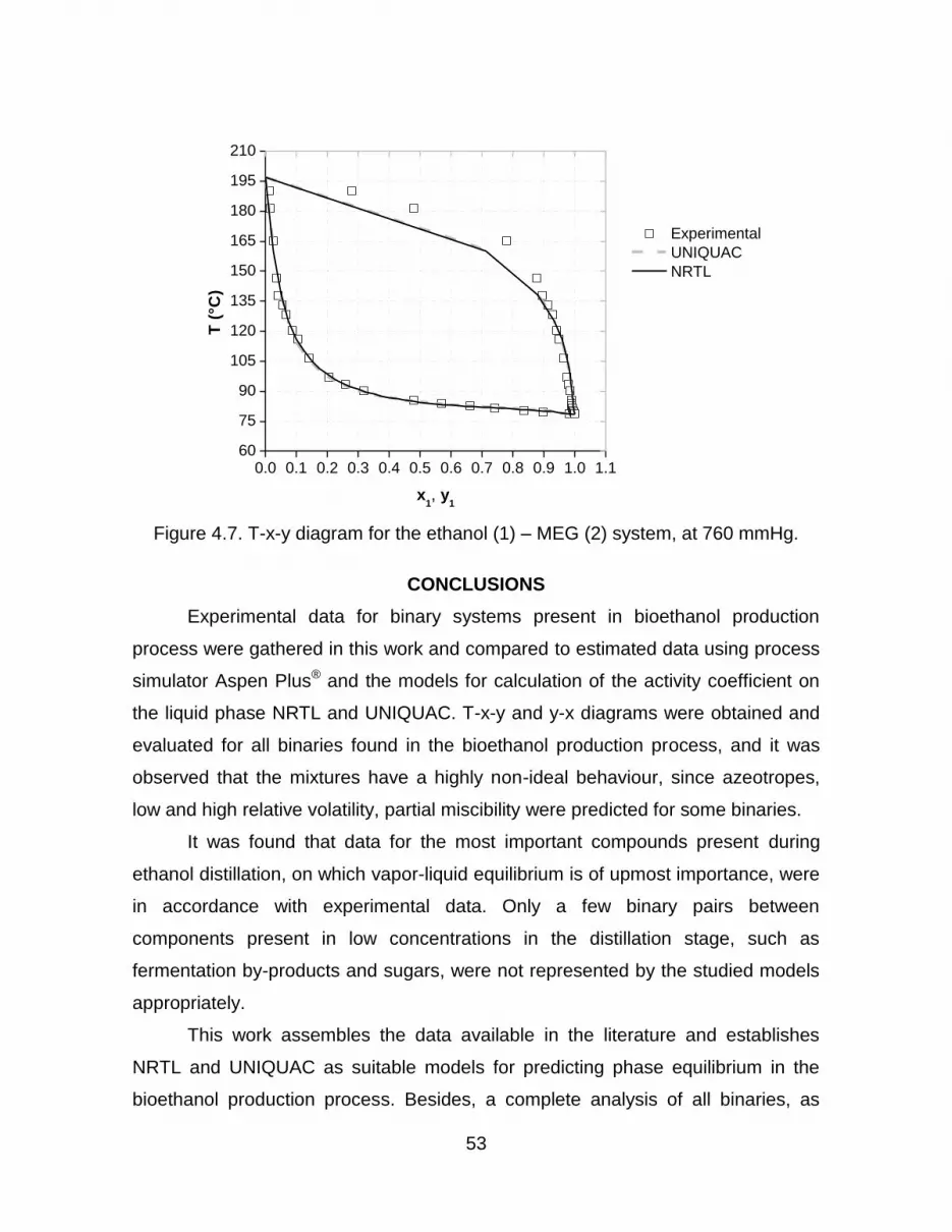
53

Figure 4.7. T-x-y diagram for the ethanol (1) – MEG (2) system, at 760 mmHg.

CONCLUSIONS

Experimental data for binary systems present in bioethanol production

process were gathered in this work and compared to estimated data using process

simulator Aspen Plus® and the models for calculation of the activity coefficient on

the liquid phase NRTL and UNIQUAC. T-x-y and y-x diagrams were obtained and

evaluated for all binaries found in the bioethanol production process, and it was

observed that the mixtures have a highly non-ideal behaviour, since azeotropes,

low and high relative volatility, partial miscibility were predicted for some binaries.

It was found that data for the most important compounds present during

ethanol distillation, on which vapor-liquid equilibrium is of upmost importance, were

in accordance with experimental data. Only a few binary pairs between

components present in low concentrations in the distillation stage, such as

fermentation by-products and sugars, were not represented by the studied models

appropriately.

This work assembles the data available in the literature and establishes

NRTL and UNIQUAC as suitable models for predicting phase equilibrium in the

bioethanol production process. Besides, a complete analysis of all binaries, as

0.0 0.1 0.2 0.3 0.4 0.5 0.6 0.7 0.8 0.9 1.0 1.160

75

90

105

120

135

150

165

180

195

210

T (

°C)

x1, y

1

Experimental

UNIQUAC

NRTL

54

showed in this work, has not been published yet and will assist the development of

other studies in this area. This study also revealed that equilibrium data are not

available for several pairs of components (e.g., 5-hydroxymethyl-furfural, pentose,

succinic acid), emphasizing the need of further experiments regarding compounds

present in bioethanol production and their phase equilibrium.


A comparação dos dados experimentais com os resultados do simulador

Aspen Plus® permitiu observar que os modelos UNIQUAC e NRTL predizem

satisfatoriamente o equilíbrio neste sistema, sendo que o NRTL apresentou

resultados ligeiramente superiores ao UNIQUAC. Observou-se ainda a

necessidade de se considerar a não-idealidade da fase vapor sendo empregada a

correlação de Hayden-O’Connell para a predição da dimerização do ácido acético

nesta fase.

Verificou-se também a ausência de dados experimentais para diversos

pares, principalmente para os que incluem componentes gerados no processo de

produção de álcool de segunda geração.

Os resultados mostraram ainda que o sistema é bastante não ideal, visto

que foram verificadas ocorrências de azeotropia, baixa e alta volatilidade relativa,

formação de duas fases líquidas entre os componentes.

Considerando-se os resultados obtidos neste capítulo, optou-se por adotar

o modelo NRTL-HOC neste trabalho, com o qual foram calculados os dados de

equilíbrios sob a forma de diagramas y-x para a pressão atmosférica apresentados

no Apêndice. Vale ressaltar que as curvas de equilíbrio representam a interação

binária entre os componentes, uma vez que o equilíbrio pode ser alterado pelo fato

do sistema ser multicomponente. Dessa forma, os diagramas foram empregados

apenas para estimar o comportamento dos componentes na coluna.

55

Capítulo 5

Avaliação dos Métodos de Cálculo para a Destilação

Convencional na Produção de Bioetanol

5.1. Introdução

Neste capítulo é apresentada a avaliação da etapa de destilação

empregada para a concentração do vinho com a finalidade de produzir bioetanol

hidratado (93 % em massa).

O processo de destilação apresenta considerável consumo de energia, a

qual é provida através da geração de vapor por meio da queima de bagaço. Como

afirmado anteriormente, o bagaço pode ser utilizado para a cogeração de

eletricidade ou para a produção de bioetanol através da hidrólise, portanto a

redução no consumo de vapor é desejável a fim de aumentar os excedentes de

bagaço. Por esta razão, a simulação do processo de destilação deve ser a mais

representativa possível a fim de que as propostas de otimização avaliadas através

desta possam ser implementadas em uma planta real.

No entanto, simuladores de processos usualmente utilizam a modelagem

de estágios de equilíbrio para realizar os cálculos das colunas de destilação. Útil

para estimativas iniciais e comparação entre configurações alternativas, esta

modelagem é baseada no conceito idealizado de estágios teóricos, embora na

prática essa suposição seja raramente aplicável. Com o intuito de considerar os

desvios do equilíbrio, a modelagem de estágios de equilíbrio pode incorporar

eficiências em seus cálculos.

Para obtenção de estimativas mais realistas, é indicado o uso da

modelagem de estágios de não equilíbrio, o qual considera as equações de

transporte que descrevem os fenômenos de transferência de massa e energia e

assume que o equilíbrio ocorre apenas na interface líquido-vapor.

Neste trabalho, utilizando-se como base a composição média do vinho

delevedurado apresentada por Dias (2008) bem como a configuração das colunas

de destilação também fornecida por esta autora, foram realizadas simulações do

56

processo de destilação através de diferentes métodos de cálculos. Foram

consideradas as modelagens de estágios de equilíbrio e de não equilíbrio bem

como a aplicação da correlação de Barros e Wolf para a determinação das

eficiências de prato e componente. A modelagem de estágios de não equilíbrio,

por ser mais rigorosa, foi utilizada como base para a avaliação dos resultados.

O desenvolvimento deste capítulo é apresentado a seguir no artigo

intitulado “Bioethanol Production Process: assessment of different calculation

methods for conventional distillation” a ser submetido a periódico internacional.

5.2. Bioethanol Production Process: assessment of different

calculation methods for conventional distillation

ABSTRACT

Distillation operation requires a significant amount of energy and, consequently, it

represents a considerable contribution to the bioethanol production costs. This is a

motivation to carry out extensive studies so that there exist incentive to simulate

this unit operation as representative as possible and the use of nonequilibrium

stage model is usually recommended since it is a rigorous calculation method.

However, most models available for simulation of multicomponent separation

processes are based on the idealized concept of equilibrium or theoretical stages.

In order to take into account the deviation from equilibrium, a usual alternative is

the consideration of efficiencies in the equilibrium stage model, thus the estimation

method of these efficiencies has considerable effects in the simulation results. In

this work, Barros & Wolf efficiency correlations for plate and component were

evaluated through comparison with nonequilibrium stage model for hydrous

bioethanol production process. It was observed that plate efficiencies are around

50 % and component efficiency is very sensitive to component properties. A

satisfactory agreement was achieved when results were compared to those

obtained using nonequilibrium stage model. Besides, constant efficiencies were

also assessed, showing that an efficiency of 70 % as global efficiency is a

reasonable estimative for this process.

57

INTRODUCTION

Bioethanol has been increasingly used as substitute or additive to gasoline,

since it is a renewable fuel and its combustion discharges less greenhouse gases

when compared to fossil-derived fuels. In Brazil, second largest producer in the

world, it is typically produced through fermentation of sugars derived from

sugarcane.

In order to be used as a fuel, wine obtained from fermentation process must

be concentrated to about 93 wt% of ethanol (hydrous bioethanol), which requires

distillation process. Besides, for bioethanol being used as gasoline additive, further

processes are necessary, since water and ethanol form an azeotrope with 95.6

wt% ethanol at 1 atm. Thus, conventional distillation cannot reach anhydrous

bioethanol specification (approximately 99.5 wt%). Azeotropic distillation with

cyclohexane as entrainer, extractive distillation with monoethyleneglycol as solvent

and adsorption onto molecular sieves are possible and usual alternatives for

bioethanol dehydration.

In view of the fact that distillation operations require a significant amount of

energy and have a great importance in bioethanol production, the simulation of this

unit operation has to be as representative as possible. However, most available

models for separation process simulation are based on the idealized concept of

equilibrium or theoretical stages, although, in practice, columns rarely operate

under thermodynamic equilibrium conditions. To take into account the deviations

from equilibrium, an efficiency value can be introduced in the calculations. In fact,

predictions can be more accurate if a nonequilibrium stage model is considered;

nevertheless the calculations are quite complex, thus taking more computational

time, which is not desirable in advanced control applications. Besides, design

parameters are needed in order to perform these calculations.

Nonequilibrium stage model of multicomponent separation processes was

first described by Krishnamurthy and Taylor (1985); their results showed that

equilibrium and nonequilibrium stage model provided predictions quite different

from each other. In the nonequilibrium stage model, conservation equations are

58

written for each phase independently and solved together with transport equations

that describe mass and energy transfers in multicomponent mixtures; also it is

assumed that equilibrium occurs only in the vapor-liquid interface. Besides, in this

way, the empirical correcting factors, such as efficiencies used in the equilibrium

model, are no longer necessary (Pescarini et al., 1996).

Several works have been developed regarding comparison between

nonequilibrium stage model and experimental data. For instance, Springer et al.

(2002) realized experiments in a bubble cap distillation column with the system

water – ethanol – methylacetate and showed that the predictions of nonequilibrium

stage model present considerably better agreement with experimental data than

those of the equilibrium stage model. In addition, Repke et al. (2004) carried out

the validation of the developed nonequilibrium stage model in a pilot packed

column and concluded that nonequilibrium stage model describes the experimental

data with a good accuracy.

Equilibrium stage model with efficiency can supply accurate results provided

that efficiencies are estimated properly. In this context, the Barros & Wolf efficiency

correlation can be used to calculate plate efficiencies for conventional distillation

columns (Wolf-Maciel et al., 2001). This correlation was obtained based on

techniques of factorial design and it is dependent on the properties of the mixture,

such as thermal conductivity, density, heat capacity and diffusivity, which vary with

efficiency. This correlation was evaluated for some systems by comparison with

results given by nonequilibrium stage model and experimental data and it was

observed that equilibrium stage model with Barros and Wolf correlation for

efficiency can represent a real nonideal process.

In this work, simulations of distillation process in bioethanol production were

carried out in Aspen Plus®, considering equilibrium stage model with constant plate

efficiency, with Barros & Wolf efficiency correlation and nonequilibrium stage

model.

59

PROCESS SIMULATION

Initial Information

The distillation process simulated was based on the traditional Brazilian

biorefineries configuration employed to produce hydrous bioethanol.

Usual configuration consists of a series of distillation and rectification

columns as depicted in Figure 5.1. Wine, produced in the fermentation stage, is fed

to column A1. Column D is responsible for removing volatile contaminants at the

top, while a large amount of water (stillage or vinasse) is obtained in the bottom of

column A. Vapor phlegm produced near to the top of column A and liquid phlegm

obtained at the bottom of column D are sent to rectification columns. The task of

the rectification consists on the concentration of the phlegm streams from 40-50

wt% to 93 wt% ethanol (hydrous bioethanol).

Figure 5.1. Configuration of the simulated process.

In Table 5.1, columns conditions and specifications are summarized. Stages

numbering is initiated in the top stage or condenser, when it is present and coupled

reboiler, as in column A, is considered the last stage. The distillation stage was

simulated considering a wine flow rate of 207 t/h, based on a distillation unit

employed in a Brazilian biorefinery.

60

Table 5.1. Distillation columns conditions and specifications

Column A

Number of stages 19 Feed stage 1 Top pressure (kPa) 139.3 Bottom pressure (kPa) 152.5 PHLEGM-V withdrawal stage 2 (vapor phase) PHLEGM-V rate (kg/h) 30000 Distillate rate (kg/h) 12750

Column A1

Number of stages 8 Feed stage: WINE TOP-A

1 8

Top pressure (kPa) 136.3 Bottom pressure (kPa) 139.3

Column D

Number of stages 6 Feed stage: REFLUX TOP-A1

1 6

Top pressure (kPa) 133.8 Bottom pressure (kPa) 136.3

Column B-B1

Number of stages 46 Feed stage: PHLEGM-L PHLEGM-V VAPOR

22 22 46

Top pressure (kPa) 116.0 Bottom pressure (kPa) 135.7 FUSEL withdrawal stages 21 and 45 (liquid phase) FUSEL rates (kg/h) 500 and 300 Distillate rate (kg/h) 16100

Wine composition, also proceeding from biorefinery data, is given in Table

5.2. This data showed that other components, such as acetaldehyde, acetone,

acetal, n-propanol, isobutanol, n-butanol and acetic acid, are also present in the

wine; however they represent less than 0.1 % in the composition and were

disregarded in this work.

61

Table 5.2. Composition of wine fed to distillation process.

Component Mass fraction

Water 0.920 Ethanol 0.073 Glycerol 0.004

Isoamyl alcohol 0.002 Glucose 0.001

Simulation Procedure

The adequacy of thermodynamic models to represent the system was

evaluated by comparison between vapor-liquid and vapor-liquid-liquid equilibrium

results given by Aspen Plus® and available experimental data (Gmehling and

Onken, 1977). Aspen Plus® simulator supplies binary parameters from its databank

and uses them automatically. Results showed that NRTL model for the activity

coefficient provides very accurate predictions. For this reason, it was used to

calculate these coefficients for the liquid phase.

Three different approaches were used in the simulation of this distillation

process regarding to column calculations: equilibrium model with constant plate

efficiencies (100, 85, 70 and 55 %), equilibrium model with Barros & Wolf efficiency

correlation for plate and component and nonequilibrium model. All simulations

considered condenser and reboiler as an equilibrium stage.

Configuration of the distillation process and specifications of the columns

were the same for all approaches. In all simulations, condenser and reboiler were

considered as equilibrium stages.

Nonequilibrium stage model simulation (NEQ)

In the nonequilibrium stage model, which is a more rigorous calculation, the

RateFracTM model was employed. This model calculates the product of the binary

mass transfer coefficients and interfacial areas using the correlations developed by

Gerster and co-workers (1958); the vapor phase and liquid phase heat transfer

coefficients are determined using the Chilton-Colburn analogy. In general, these

quantities depend on column diameter and operating parameters. Tray type was

defined as bubble cap and column diameter was calculated based on the approach

of flooding on the stage where it is most critical (Aspen Technology, 2001).

62

Parameters used in calculations, such as vapor and liquid flows, densities,

viscosities, surface tension of liquid, vapor and liquid phase binary diffusion

coefficients, are all estimated through equations present in Aspen Plus®.

Equilibrium stage model simulation with constant efficiency (EQ)

In order to perform equilibrium stage model simulations, RadFracTM model in

Aspen Plus® software is used, which performs calculation using the MESH

equations (mass, equilibrium, summation and heat). In this case, number of stages

and feed inlet positions are specified together with the specification given in Table

5.1. Efficiencies were inserted as Murphree efficiency and were considered the

same for all stages: 100, 85, 70 and 55 % in cases EQ100, EQ85, EQ70 and

EQ55, respectively.

Equilibrium stage model simulation with Barros & Wolf efficiency correlation (Eff)

For these simulations, column distillation model is also RadFracTM

(equilibrium calculation). In this case, number of stages and feed inlet positions are

specified as well as the efficiencies calculated through Barros & Wolf correlation

(Equation 5.1), which are included as Murphree efficiencies (Barros, 1997).

04516.0

2 )()(

)()()()(5309.38)(

iiCp

iMWiDiikiEff (5.1)

In Equation 5.1, Eff(i) is the plate efficiency (Eff-plate) described as a

function of the following mixture properties in each stage (i): thermal conductivity

(k), density ( ), diffusivity (D), molecular weight (MW), heat capacity (Cp) and

viscosity ( ). These properties are calculated for all stages in the distillation

columns using Aspen Plus®. For component efficiencies (Eff-comp), instead of

mixture properties in the plate, individual component properties are considered in

Equation 5.1.

The determination of these efficiencies is an iterative method, since the first

simulation is carried out using an efficiency of 100 %, then the calculated

properties are used to predict efficiencies through Barros & Wolf correlation.

Subsequently, these efficiencies are inserted in the simulation and the properties

are recalculated, thus new efficiencies values are obtained. This procedure is

repeated until the difference between two consecutive efficiency iterations reaches

63

a level of tolerance below 1.10-4. Generally, three iterations are enough to

determine efficiencies within the specified tolerance.

RESULTS AND DISCUSSION

Sidestream Withdrawal

Since fusel oil has a significant commercial value, its recovery is essential to

the process. Fusel oil (FUSEL stream) consists of heavy alcohols, such as isoamyl

alcohol. The fusel oil withdrawal position was determined by analysing isoamyl

alcohol mass fraction in liquid phase using equilibrium model as base case.

Column B-B1 composition profiles can be seen in Figure 5.2.

Figure 5.2. Isoamyl alcohol mass fraction profile in column B-B1 for equilibrium

model simulation.

From Figure 5.2 can be observed that stages 21 and 45 present the highest

mass fractions of isoamyl alcohol, thus sidestreams were withdrawn from these

stages.

Nonequilibrium Stage Model

Simulation using nonequilibrium stage model presented more convergence

problems and took more time to provide results when compared to other models,

which was expected since it takes into account more equations. For instance,

equilibrium calculation solves 2nc+1 equations for each stage while nonequilibrium

0.00

0.02

0.04

0.06

0.08

0.10

0.12

0.14

1 6 11 16 21 26 31 36 41 46

Stage

Mas

s F

racti

on

top bottom

64

solves 5nc+3 equations, where nc is the number of components (Pescarini et al.,

1996), consequently, 11 and 28 equations, respectively, per stage in the situation

considered in this work.

Since nonequilibrium stage model takes into account mass and energy

transfer phenomena, it is more rigorous and complex than equilibrium stage model.

In addition, predictions given by nonequilibrium model are usually more accurate

when compared to experimental results (Repke et al., 2004; Springer et al., 2002).

For these reasons, it will be used to evaluate other calculation approaches

considered in this work.

Main stream results obtained with nonequilibrium stage model are shown in

Table 5.3.

Table 5.3. Main stream results given by nonequilibrium model.

Stream STILLAGE PHLEGMAS ETHANOL FUSEL1 FUSEL2

Temperature (°C) 111.9 106.0 81.7 93.1 100.9

Mass Flow (kg/h) 175347.2 14693.2 16100.0 500.0 300.0

Water (wt%) 99.4 98.8 7.0 48.3 62.2

Glucose (wt%) 0.1 - - - -

Ethanol (wt%) - - 93.0 25.0 0.2

Glycerol (wt%) 0.5 - - - -

Isoamyl alcohol (wt%) - 1.1 0 26.7 37.6

From Table 5.3, it can be inferred that hydrous bioethanol production was

16.1 t//h and its concentration was around 93 wt% ethanol. Stillage and

phlegmasse (“STILLAGE and “PHLEGMAS” in Figure 5.1) do not present ethanol

and are basically water. Besides, fusel oil streams – “FUSEL1” and “FUSEL2” –

have a considerably amount of isoamyl alcohol as desired in this process.

Although all columns were simulated using nonequilibrium stage model, in

this work, column B-B1 is used to summarize the results of this study. Column B-

B1 has larger number of stages and, as a result, it is the most influenced column in

this process, concerned with the objectives of this work. Temperature profile is

given in Figure 5.3.

It can be observed that liquid and interface temperature profiles obtained in

the NEQ model were coincident, indicating that there is no resistance to energy

transfer between interface and liquid phase. However, vapor temperatures

65

calculated by NEQ slightly diverged from the other temperatures, which means that

vapor phase controls energy transfer in the system.

Figure 5.3. Temperature profile for column B-B1 using nonequilibrium stage model.

Equilibrium Stage Model with Constant Efficiency

Simulations considering equilibrium stage model with constant plate

efficiencies were carried out in order to evaluate whether a constant efficiency can

provide predictions similar to nonequilibrium stage model. Temperature profile,

depicted in Figure 5.4, was used to illustrate the comparison between these

models.

Figure 5.4. Temperature profile using equilibrium stage model with constant plate

efficiencies and nonequilibrium stage model.

80

85

90

95

100

105

1 6 11 16 21 26 31 36 41 46

Stage

Tem

pera

ture

(°C

)Liquid Interface Vapor

top bottom

80

85

90

95

100

105

1 6 11 16 21 26 31 36 41 46

Stage

Te

mp

era

ture

(°C

)

NEQ EQ55 EQ70 EQ85 EQ100

top bottom

66

It can be inferred from Figure 5.4 that the curve given by EQ100 (ideal

situation) considerably deviates from the one given by NEQ. Besides, analyzing

temperatures given by equilibrium model with constant plate efficiency (EQ55,

EQ70 and EQ85), it can be observed that temperatures are higher for the superior

values of efficiency, since this cases are closer to the ideal situation, hence it

follows that energy transfer is not as restrictive as in nonequilibrium model. Among

simulations considering plate efficiency, taking NEQ simulation as base, EQ70

predicted better results since its curve is the closest to NEQ along the entire

column. Therefore, efficiency of 70 % is a reasonable value for efficiency in this

process.

Concerning energy requirements, Figure 5.5 presents the comparison

between cases studied. It is important to emphasize that, in this process, energy

consumption is the amount of energy required in the reboilers of columns A and B-

B1, which, in practice, is provided through heat exchange between process steam

and the bottom product to be evaporated.


equilibrium stage model with constant plate efficiencies and nonequilibrium stage

model.

Analyzing Figure 5.5, it was observed that energy consumptions presented

not significant variations, since the values were between 26.7 and 26.9 Gcal/h.

Besides, it can be verified that the energy consumption increases with the

26.70

26.75

26.80

26.85

En

erg

y c

on

su

mp

tio

n (

Gcal/h

)

EQ55 EQ70 EQ80 EQ100 NEQ

Case

67

efficiency. At first, it can seem contradictory, given that, for a fixed number of

stages, lower efficiencies require higher reflux rates and, consequently, larger

energy requirements if the product specification is the same. However, in this case,

product specification was not fixed, but the column parameters were. Therefore,

this behavior can be associated to the stage temperatures, which also increases

with efficiency as shown in Figure 5.4.

Equilibrium Stage Model with Barros & Wolf Efficiency Correlation

Values obtained for plate and component efficiency across column B-B1 are

displayed on Figure 5.6. Water, ethanol, and isoamyl alcohol efficiencies are

between 0.45 and 0.60, whereas glycerol presents higher efficiencies, around 0.7,

and glucose efficiencies vary between 1.2 and 1.7. These results indicate that

efficiency is higher for low-volatile components, which also present high viscosity

and are mostly found in liquid phase inside the column. Plate efficiencies are

situated between water and ethanol efficiencies, since these components are

found in higher concentration in column B-B1, presenting values around 0.50.

Figure 5.6. Efficiency profile in column B-B1.

Temperature profiles for equilibrium stage model with Barros & Wolf

efficiency correlation for plate and component and nonequilibrium stage model are

illustrated in Figure 5.7.

0.4

0.6

0.8

1.0

1.2

1.4

1.6

1.8

2 6 10 14 18 22 26 30 34 38 42 46

Stage

Eff

icie

ncy

Water Glucose Ethanol Glycerol Isoamyl alcohol Plate

top bottom

68

Figure 5.7. Temperature profile using equilibrium model with Barros & Wolf

efficiency correlation for plate and component and nonequilibrium stage model.

Equilibrium stage model with Barros & Wolf correlation efficiency provided

reasonable temperature values when compared to nonequilibrium stage model;

moreover curve generated considering plate efficiency was closest to that given by

nonequilibrium stage model.

Energy requirements for equilibrium model with Barros & Wolf efficiency

correlation for plate (Eff-plate) and component (Eff-comp) were also evaluated and

comparison with nonequilibrium model results is shown in Figure 5.8 In this case, it

can be noticed that energy consumptions were not significantly different from

results of nonequilibrium stage model, and simulation using plate efficiency

presented more similar results than that using component efficiency.

80

85

90

95

100

105

1 6 11 16 21 26 31 36 41 46

Stage

Tem

pera

ture

(°C

)

NEQ Eff-plate Eff-comp

top bottom

69


equilibrium model with Barros & Wolf efficiency correlation for plate and component

and nonequilibrium model.

The superiority of plate efficiency over component efficiency to predict

temperatures and energy consumptions can be explained by the fact that plate

efficiencies take into account mixture properties while component efficiencies use

only individual properties. The effect of the mixture in the plate is essential to

column behaviour; consequently, a correlation that uses its properties is generally

more accurate.

Summary of Results

Comparison between results given by equilibrium stage model (efficiency of

100 %), equilibrium model with Barros & Wolf correlation efficiency for plate and

component and nonequilibrium model is presented through composition profiles

(vapor and liquid) depicted in Figures 5.9 and 5.10. In order to simplify the analysis

of composition profiles, only water and ethanol mole fraction are shown, since they

present higher concentration inside the column.

26.70

26.75

26.80

26.85

26.90

26.95

27.00

En

erg

y c

on

su

mp

tio

n (

Gca

l/h

)

NEQ Eff-plate Eff-comp

Case

70

Figure 5.9. Composition profile for vapor phase considering equilibrium model with



Figure 5.10. Composition profile for liquid phase considering equilibrium model with


nonequilibrium model.

From examination of Figures 5.9 and 5.10, it is possible to observe that

equilibrium stage model with Barros and Wolf efficiency correlations (Eff-plate and

0.0

0.1

0.2

0.3

0.4

0.5

0.6

0.7

0.8

0.9

1 6 11 16 21 26 31 36 41 46

Stage

Va

po

r m

ole

fra

cti

on

EQ100 NEQ Eff-plate Eff-comp

Water

Ethanol

top bottom

0.0

0.1

0.2

0.3

0.4

0.5

0.6

0.7

0.8

0.9

1.0

1 6 11 16 21 26 31 36 41 46

Stage

Liq

uid

mo

le f

rac

tio

n

EQ100 NEQ Eff-plate Eff-comp

Water

Ethanol

top bottom

71

Eff-comp) provides a composition profile more accurate taking nonequilibrium

model as base.

Energy demand was also compared and results are shown in Table 5.4.

Table 5.4. Comparison between energy requirements.

Case Energy consumption

(Gcal/h) Relative

Difference (%)

Nonequilibrium model 26.85 - Equilibrium model with Barros & Wolf

correlation plate efficiency 26.95 0.37

Equilibrium model with Barros & Wolf correlation component efficiency

26.98 0.50

Equilibrium model (ideal situation) 26.82 - 0.12

Although equilibrium stage model showed results more similar to

nonequilibrium regarding energy requirements, relative differences between results

are not significant, since they are less than 1 %. Besides, it can be seen that

equilibrium stage model calculates slightly lower energy consumption when

compared with other calculation methods, because it assumes that vapor and

liquid phases leave stages in equilibrium. Once mass and energy transfers or

efficiency are considered, as in nonequilibrium stage model and equilibrium stage

model with efficiency, more stages and energy are required to achieve the same

separation.

CONCLUSIONS

Simulations of bioethanol production process were carried out considering

equilibrium with constant efficiency, with plate and component correlation efficiency

and nonequilibrium stage models. Literature review showed that nonequilibrium

stage model predicts results in good agreement with experimental results,

however, further studies including experiments are recommended to validate

nonequilibrium stage model for bioethanol production process. In this work,

nonequilibrium stage model was used as base to evaluate equilibrium stage model

with efficiency.

In the nonequilibrium stage model, liquid, vapor and interface temperature

profiles were analysed; liquid phase and interface temperatures were coincident,

72

while vapor phase presented a deviation from interface temperatures, which

means that the liquid phase presents no resistance to energy transfer and the

vapor phase controls this process.

Results obtained considering equilibrium model with constant plate

efficiency indicated that efficiency of 70 % is a good estimative for this process,

since a satisfactory agreement was achieved between temperature profiles.

Equilibrium model with efficiency of 100 % presented significant deviations in

temperature profile as well as in composition profiles.

Plate efficiencies determined through Barros & Wolf efficiency correlation

are around 50 % and component efficiencies are found in a range between 0.4 and

1.7, presenting higher values for low-volatile components. Simulation results with

equilibrium stage model with plate and component efficiency, determined by Barros

and Wolf correlation, showed a good agreement with results predicted by the


Energy requirements were evaluated for equilibrium model with efficiency of

100 %, with plate and component efficiency and nonequilibrium model and it can

be concluded that there is no considerable difference between the predicted

values.


Neste capítulo foram avaliadas diferentes abordagens para o cálculo de

colunas de destilação empregadas no processo de produção de bioetanol.

A modelagem de estágios de equilíbrio forneceu perfis de temperatura para

as fases líquida e vapor e também para a interface. Observou-se que a fase

líquida e a interface apresentam curvas coincidentes, enquanto a curva relativa à

fase vapor distancia-se destas. Desta forma, pode-se afirmar que a fase líquida

não oferece resistência à transferência de energia e a fase vapor controla este

processo.

A comparação entre a modelagem de equilíbrio com eficiência constante

com a modelagem de não equilíbrio indicou que eficiência de 70 % é uma

estimativa razoável para este processo. No entanto, eficiências de prato

73

calculadas pela correlação de Barros e Wolf mantiveram-se em torno de 50 % e as

eficiências de componente variaram entre 40 e 170 %, sendo maiores para

componentes de baixa volatilidade. Resultados preditos utilizando a modelagem

de estágios de equilíbrio com eficiências determinadas pela correlação de Barros

e Wolf apresentaram concordância satisfatória quando comparada à modelagem

de não equilíbrio.

Vale ressaltar que o processo de concentração do etanol é composto por

colunas de destilação e retificação, possuindo múltiplas alimentações e saídas

laterais. Além disso, a consideração de um sistema multicomponente bem como a

interação entre as colunas através de reciclos tornam a aplicação da correlação de

eficiência mais complexa.

74

Capítulo 6

Avaliação dos Métodos de Cálculo para a Destilação

Extrativa na Produção de Bioetanol

6.1. Introdução

Com a finalidade de ser misturado à gasolina, bioetanol deve ser

desidratado de forma a atingir a especificação de 99,5 % etanol (em massa).

Assim, o bioetanol hidratado produzido através da destilação convencional deve

ser submetido a processos posteriores de separação que sejam capazes de obter

bioetanol com concentração de etanol maior que a do azeótropo (95,6 %). No

Brasil, dentre os processos de desidratação destacam-se a destilação azeotrópica

com cicloexano e a destilação extrativa com monoetilenoglicol. Apesar de a

destilação azeotrópica ser a mais utilizada atualmente, tem-se que a destilação

extrativa é superior no que se refere à facilidade de operação e ao consumo de

vapor de processo, o qual é consideravelmente menor neste último processo.

Assim como para a destilação convencional, os cálculos para a destilação

extrativa podem ser realizados utilizando modelagens de estágios de equilíbrio e

de não equilíbrio bem como podem ser inseridos valores de eficiência de prato e

componente. Neste contexto, considerando-se como alimentação o produto da

destilação descrita na seção 5.2, foram realizadas simulações do processo de

destilação extrativa com monoetilenoglicol considerando os diferentes métodos.

Além disso, o uso da correlação de eficiência de Barros e Wolf para destilação

extrativa foi avaliado através de comparação com a modelagem de não equilíbrio.

O desenvolvimento deste capítulo é apresentado a seguir no artigo

intitulado “Simulation of extractive distillation process in bioethanol production

using equilibrium stage model with efficiency and nonequilibrium stage model” a

ser submetido a periódico internacional.

75

6.2. Simulation of extractive distillation process in bioethanol

production using equilibrium stage model with efficiency and

nonequilibrium stage model

ABSTRACT

In view of the increasing environmental concern, the use of renewable and less

pollutant energy sources has been encouraged. In this context, bioethanol has

been used as fuel in the anhydrous form, blended with gasoline. In this work,

simulations of extractive distillation process in anhydrous bioethanol production

were carried out in Aspen Plus® using nonequilibrium stage model and equilibrium

stage model with Barros & Wolf efficiency correlations for plate and component.

Equilibrium stage model with plate efficiency determined through Barros & Wolf

efficiency correlation showed a satisfactory agreement with results predicted by

nonequilibrium stage model for anhydrous bioethanol production process.

INTRODUCTION

Recently, global concern about climate change has motivated the use of

alternative forms of energy all over the world. In the transportation sector, more

specifically, bioethanol and biodiesel have been increasingly used as substitutes of

gasoline and diesel, respectively.

Bioethanol is mainly produced from fermentation of sugars, which generates

wine containing about 7-12 wt% ethanol. In order to be used as a gasoline additive,

wine must be concentrated at least to 99.5 wt% ethanol. Initially, conventional

distillation is employed to concentrate wine up to 93 wt%, which is near the

azeotropic composition (95.6 wt% of ethanol). Subsequently, further operations are

required to produce anhydrous bioethanol, such as azeotropic distillation with

cyclohexane and extractive distillation with ethyleneglycol (EG).

In spite of being the most common dehydration process, azeotropic distillation

with cyclohexane presents several disadvantages, such as high energy consumption

on columns reboilers, use of a harmful, flammable, toxic and fossil separation agent

76

(Rivière and Marlair, 2009) and product contamination with solvent, besides its

operation is quite complex due to formation of two liquid phases in some of internal

plates (Junqueira et al., 2009). Although extractive distillation with EG also makes

use of a fossil and harmful separating agent, it is still advantageous since it requires

less energy and it is easier to operate.

For any distillation-based process, it is essential to ensure appropriate design

of distillation columns to guarantee that the separation desired is achieved, otherwise

it can have considerable environmental and economic implications. In order to design

a column, number of stages and operational conditions are required; in this context,

simulation softwares are useful tools. However, simulation accuracy deeply relies on

the type of model used for calculations. Most available simulation softwares are

based on the equilibrium stage model (EQ) calculations, which is an idealized model

that assumes the achievement of thermodynamic equilibrium between the contacting

phases. In practice, the contact time between the vapor and liquid phases is not long

enough for equilibrium to be established. In this context, it is, therefore, desirable to

consider the deviation from equilibrium through introduction of efficiency. Another

possible alternative is the use of nonequilibrium stage model (NEQ), also called rate-

based. This type of model, though complicated relative to the equilibrium model, it

provides a realistic estimate of the distillation column performance without

incorporating efficiency factors.

In this work, simulations of bioethanol dehydration process through extractive

distillation with ethyleneglycol were carried out in Aspen Plus®. Nonequilibrium stage

model and equilibrium stage model with application of an efficiency correlation were

used to perform calculations.

EXTRACTIVE DISTILLATION PROCESS

Extractive distillation, also known as homogeneous azeotropic distillation, is

commonly used to separate nonideal mixtures with close boiling point or azeotropes.

In this process, a heavy boiling solvent is added to the system to be separated, which

alters the volatility of the component in the original mixture. New azeotropes must not

be formed and the solvent must be completely miscible in the mixture, in other words,

77

it must not form a second liquid phase as in heterogeneous azeotropic distillation

(Dias et al. 2009a; Reis et al., 2006).

In the conventional configuration employed in bioethanol production process,

solvent and the water-ethanol mixture (HE, hydrous ethanol) are fed to the first

column (extractive column). Anhydrous ethanol is produced on the top of the

extractive column, while in the bottom a mixture containing solvent and water is

obtained. The solvent is recovered in a second column (recovery column), cooled

and recycled to the extractive column (Huang et al., 2008).

Meirelles et al. (1992) demonstrated that ethyleneglycol (EG) is an efficient

solvent for anhydrous bioethanol production by extractive distillation. This process

was first employed in industrial scale in Brazil in the 2001 sugarcane harvest season,

and is today one of the most common processes for ethanol dehydration.

Comparing with conventional distillation process, extractive distillation has

larger number of degrees of freedom. In a simple distillation setup, these degrees of

freedom are the reflux ratios and the number of stages of the distillation columns. For

extractive distillation, the solvent choice and the solvent flow rate comprise additional

degrees of freedom (Kossack et al, 2007).

NONEQUILIBRIUM STAGE MODEL

The development of the rigorous nonequilibrium stage model, described by

Krishnamurthy and Taylor (1985), considers each phase to be separated by an

interface through which heat and mass transfer occur. Consequently, conservation

equations are written for each phase independently and solved together with

transport equations that describe mass and energy transfers in multicomponent

mixtures; also it is assumed that equilibrium occurs only in the vapor-liquid

interface (Pescarini et al., 1996).

While the nonequilibrium model is more rigorous, it can also become more

difficult to implement for dynamic simulations, optimization and control. In addition,

some parameters of the model such as the mass transfer coefficients may be

difficult to estimate accurately (Pradhan and Kannan, 2005).

Pradhan and Kannan (2005) analyzed extractive distillation process through

nonequilibrium stage model and concluded that purity in the distillate is significant

78

lower than that predicted by equilibrium stage model. Additionally, it was observed

that the idealized model requires fewer stages to achieve the same purity obtained

using the rate-based model.

Nava and Krishna (2004) examined the influence of interphase mass

transfer on the composition trajectories in extractive distillation. They highlighted

the need of adopting nonequilibrium stage model in this process, since their results

showed the superiority of NEQ over equilibrium stage model regarding prediction

of column composition trajectories.

Castillo and Towler (1998) also studied the influence of mass transfer in the

extractive distillation by analysis of residue-curve maps. The authors noticed that

NEQ affects the curvature of boundaries and, occasionally, EQ might allow design of

distillation sequence that is unfeasible once mass transfer is taken into account. In

these cases, not even the overdesign, which can include extra trays or additional

reflux, can overcome this miscalculation.

Nonequilibrium stage model has been incorporated into the commercially

available software Aspen Plus® through the package RateFracTM. This model

calculates the product of the binary mass transfer coefficients and interfacial areas

using the correlations developed by Gerster and co-workers (1958); the vapor and

liquid phase heat transfer coefficients are determined using the Chilton-Colburn

analogy. In general, these quantities depend on column diameter and operating

parameters. Parameters used in calculations, such as vapor and liquid flows,

densities, viscosities, surface tension of liquid, vapor and liquid phase binary

diffusion coefficients, are all estimated through well known equations included in

Aspen Plus® (Aspen Technology, 2001).

EFFICIENCY CORRELATIONS

As stated previously, through equilibrium stage model is not possible to predict

accurately extractive distillation since heat and mass transfer mechanisms must be

taken into account. Towards this end, an alternative way to correct this weakness is

the application of efficiency correlations.

In this context, efficiency correlations for plate and component in conventional

and extractive distillations were evaluated (Barros, 1997; Wolf-Maciel et al., 2001;

79

Reis et al., 2006). These correlations, known as Barros and Wolf efficiency

correlation, were obtained based on techniques of factorial design and present the

relation between efficiency and the properties of the mixture, such as thermal

conductivity, density, heat capacity and diffusivity, which vary with efficiency.

Barros and Wolf plate correlation and the component efficiency correlation for

conventional (Equations 6.1 and 6.2) and extractive distillation (Equations 6.3 and

6.4) are displayed below.

04516.0

2 )()(

)()()()(5309.38)(

iiCp

iMWiDiikiEff (6.1)

04516.0

2 ),(),(

)(),(),(),(5309.38),(

jijiCp

jMWjiDjijikjiEff (6.2)

109588.0

2 )()(

)()()()(37272.19)(

iiCp

iMWiDiikiEff (6.3)

109588.0

2 ),(),(

)(),(),(),(37272.19),(

jijiCp

jMWjiDjijikjiEff (6.4)

In these equations, Eff(i) is the plate efficiency in plate i and Eff(i,j) is the

efficiency of component j on plate i. The equations are function of thermal

conductivity (k), density ( ), diffusivity (D), molecular weight (MW), heat capacity

(Cp) and viscosity ( ). For calculation of plate efficiencies, properties of the mixture

in the plate are considered, whereas for component efficiency, the pure component

properties in the plate are used.

Reis et al. (2006) performed calculations using a computational program in

Fortran language to simulate extractive distillation columns using equilibrium stage

model. In this program, a subroutine to calculate efficiency through Barros and

Wolf correlations was included. The simulation results were compared to those

calculated using NEQ and also with experimental data of a pilot-scale extractive

distillation column. A satisfactory agreement was achieved, showing that the

efficiency correlations are reliable and applicable to extractive distillation process.

80

In Aspen Plus®, calculations of equilibrium stage model are realized through

RadFracTM model. This model allows the inclusion of Murphree efficiencies and

vaporization efficiencies for plate and components (Aspen Technology, 2001).

SIMULATION PROCEDURE

For calculations, NRTL model was used for the estimation of activity

coefficients and vapor phase was considered ideal. Configuration of the distillation

process to produce anhydrous bioethanol (AE) is depicted in Figure 6.1. Column

specifications are given in Table 6.1. All simulations considered the same

configuration and columns specifications, besides condenser and reboiler were

considered as equilibrium stages for all calculation approaches.

Figure 6.1. Configuration of extractive distillation process with ethyleneglycol.

Table 6.1. Specifications in the extractive and recovery columns (mass basis).

Specification Extractive Column Recovery Column

Number of Stages 32 18

Pressure (kPa) 101.3 50

Feed Position Solvent 3

HE 24 9

Condenser Type Partial Partial

Solvent to Feed Ratio 0.62 -

Reflux Ratio 1.05 0.38

Distillate Rate (kg/h) 15051 -

Bottoms Rate (kg/h) - 9984.0

ECRC

SOLVENT

HE

AE

WATER

TO-REC

EG

PUMPCOOLERMIXER

MAKE-UP

81

Firstly, simulations were performed using nonequilibrium stage model, which

makes use of RateFracTM model in Aspen Plus®, with the purpose of obtaining

anhydrous bioethanol (99.5 wt% ethanol). Tray type was defined as bubble cap and

column diameter was calculated based on the approach of flooding on the stage

where it is most critical.

Secondly, calculations considering equilibrium stage model (RadFracTM) were

carried out without addition of efficiency values, which means an efficiency of 100 %

(ideal situation). Finally, in order to include efficiency in equilibrium calculations,

properties were retrieved from the previous simulation and used to calculate the initial

values of efficiency through Barros and Wolf efficiency correlation. For the extractive

column it was employed the correlation for extractive distillation, while for the

recovery column it was used the correlation for conventional distillation.

Subsequently, these efficiencies were inserted in the simulation as Murphree

efficiencies and the properties were recalculated, thus obtaining new efficiencies

values. This procedure was repeated until the difference between two consecutive

efficiency iterations reached a level of tolerance below 1.10-4. Generally, three

iterations are enough to determine efficiencies within the specified tolerance. The

procedures for plate and component efficiency are similar, except for the equation

used.


Tables 6.2 to 6.5 present the main stream results for the different approaches

considered in this study.

Table 6.2. Main stream results using nonequilibrium stage model.

Stream AE SOLVENT WATER TO-REC

Temperature (°C) 78.4 110 82.2 139

Pressure (bar) 1.0 1.0 0.5 1.0

Mass Flow (kg/h) 15051 9989.0 1054.0 11038

Ethanol (wt%) 99.5 - - -

Water (wt%) 0.5 - 99.8 9.5

Ethyleneglycol (wt%) - 100 0.2 90.5

82

Table 6.3. Main stream results using equilibrium stage model.


Temperature (°C) 78.3 110 83.5 139.1 Pressure (bar) 1.0 1.0 0.5 1.0

Mass Flow (kg/h) 15051 9989.0 1054.0 11038 Ethanol (wt%) 99.5 - - - Water (wt%) 0.5 - 99.6 9.5


Table 6.4. Main stream results using equilibrium stage model with plate efficiency.


Temperature (°C) 78.4 110 82.0 138 Pressure (bar) 1.0 1.0 0.5 1.0

Mass Flow (kg/h) 15051 9989.0 1054.0 11038 Ethanol (wt%) 99.4 - 1.3 0.1 Water (wt%) 0.6 - 98.5 9.4


Table 6.5. Main stream results using equilibrium stage model with component

efficiency.


Temperature (°C) 78.3 110 81.9 135 Pressure (bar) 1.0 1.0 0.5 1.0

Mass Flow (kg/h) 15051 9989.0 1054.0 11038 Ethanol (wt%) 99.0 - 7.3 0.7 Water (wt%) 1.0 - 92.5 8.8


From analysis of main stream results, it is possible to observe that NEQ, EQ

and EQ with plate efficiency are in better agreement regarding stream

temperatures than the simulation with component efficiency. Concerning stream

composition, EQ and simulation with plate efficiency provided satisfactory results

when compared to NEQ. EQ with component efficiency did not present reasonable

results probably due to lack of mixture properties in the equation that can lead to

miscalculations. Although EQ is an idealized model, it provided reasonable

prediction when compared to NEQ, which can be explained by the large number of

stages due to the demanding specification (93 wt% ethanol). In other words, if

83

number of stages were determined to achieve separation considering EQ, NEQ

results would be quite different since it requires a larger number of stages to

perform the same separation.

Energy requirements were also evaluated and comparison between results

for all approaches is displayed in Table 6.6.

Table 6.6. Energy requirements for all calculation methods.

Calculation Method

Energy Requirement (Gcal/h)

NEQ EQ EQ with Plate

Efficiency EQ with Component

Efficiency

Condenser-EC -3.26 -3.22 -3.25 -3.26

Reboiler-EC 2.91 2.87 2.89 2.91

Condenser-RC -0.21 -0.22 -0.21 -0.20

Reboiler-RC 0.99 1.00 0.98 0.98

Energy requirements predicted by different models were quite similar, with

EQ presenting the larger deviations, which was expected since this model does not

take into account mass and heat transfer mechanisms.

In order to analyze column profiles, results of extractive and recovery

columns are presented apart from each other.

Extractive Column (EC)

Plate and component efficiencies determined by Barros and Wolf correlation

for extractive distillation are shown in Figure 6.2. It can be observed that

efficiencies are between 0.30 and 0.60, presenting disturbances in solvent and

azeotropic feed positions (stages 3 and 24). Plate efficiencies are located between

component efficiencies and water presents lowest efficiency values and EG the

largest ones. These observations are in accordance with results obtained by Reis

et al. (2006).

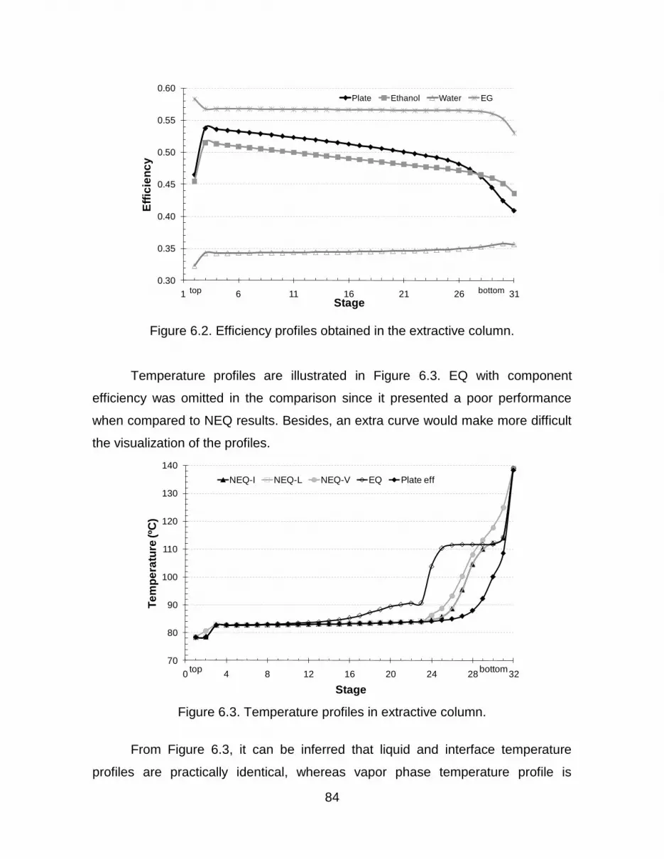
84

Figure 6.2. Efficiency profiles obtained in the extractive column.

Temperature profiles are illustrated in Figure 6.3. EQ with component

efficiency was omitted in the comparison since it presented a poor performance

when compared to NEQ results. Besides, an extra curve would make more difficult

the visualization of the profiles.

Figure 6.3. Temperature profiles in extractive column.

From Figure 6.3, it can be inferred that liquid and interface temperature

profiles are practically identical, whereas vapor phase temperature profile is

0.30

0.35

0.40

0.45

0.50

0.55

0.60

1 6 11 16 21 26 31

Eff

icie

nc

y

Stage

Plate Ethanol Water EG

top bottom

70

80

90

100

110

120

130

140

0 4 8 12 16 20 24 28 32

Te

mp

era

ture

(ºC

)

Stage

NEQ-I NEQ-L NEQ-V EQ Plate eff

top bottom

85

different, which means that there is no resistance to energy transfer between

interface and liquid phase, while vapor phase controls energy transfer in the

system. Therefore, it can be concluded that the supposition of equality of all

temperatures as considered in the equilibrium stage model is not a reasonable

approximation for this system.

Although none of equilibrium stage model presented a satisfactory

agreement with NEQ as shown in Figure 6.3, EQ with plate efficiency provided

prediction with smaller deviations as well as a behavior more similar to NEQ than

the idealized equilibrium stage model.

In respect to composition profile, vapor mole fractions along the column are

given in Figure 6.4. Ethyleneglycol mole fraction was omitted from this profile since

its values were normally around zero. Analyzing the curve given by EQ, it can be

seem that the last stages have no function since the composition does not vary

between stages 25 and 31, which means that the column is overdesigned for the

equilibrium situation. Therefore, curves predicted by EQ and NEQ have the same

initial and final values, although the curves follow different tendencies.

On the other hand, EQ with plate efficiency presented tendency analogous

to that of the NEQ. In addition, vapor mole fraction predicted by EQ with plate

efficiency also presented coincident values in the top and bottom of the column

when compared to NEQ.

Figure 6.4. Composition profiles for vapor phase in extractive column.

0.0

0.2

0.4

0.6

0.8

1.0

1.2

0 4 8 12 16 20 24 28 32

Va

po

r M

ole

Fra

cti

on

Stage

Ethanol-NEQ Water-NEQ Ethanol-EQ

Water-EQ Ethanol-Plate Eff Water-Plate Eff

top bottom

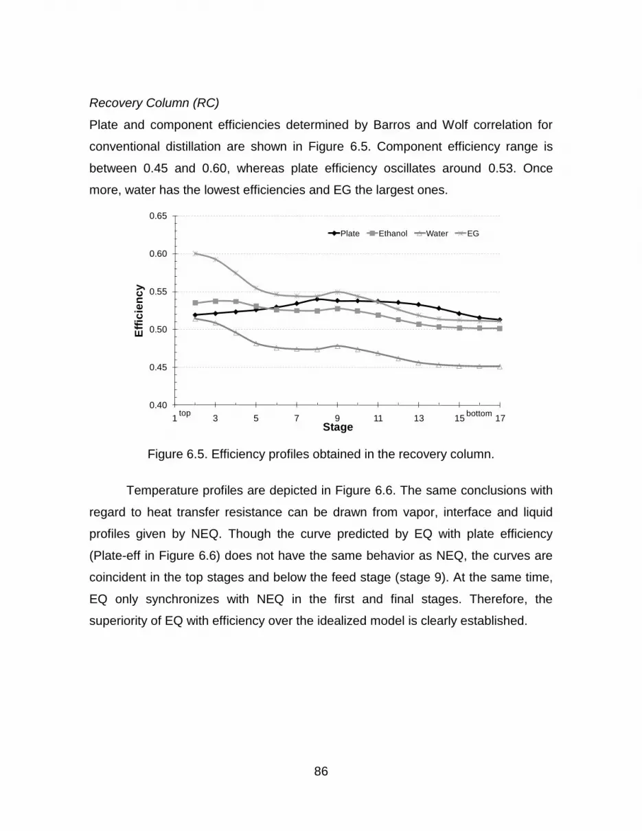
86

Recovery Column (RC)

Plate and component efficiencies determined by Barros and Wolf correlation for

conventional distillation are shown in Figure 6.5. Component efficiency range is

between 0.45 and 0.60, whereas plate efficiency oscillates around 0.53. Once

more, water has the lowest efficiencies and EG the largest ones.

Figure 6.5. Efficiency profiles obtained in the recovery column.

Temperature profiles are depicted in Figure 6.6. The same conclusions with

regard to heat transfer resistance can be drawn from vapor, interface and liquid

profiles given by NEQ. Though the curve predicted by EQ with plate efficiency

(Plate-eff in Figure 6.6) does not have the same behavior as NEQ, the curves are

coincident in the top stages and below the feed stage (stage 9). At the same time,

EQ only synchronizes with NEQ in the first and final stages. Therefore, the

superiority of EQ with efficiency over the idealized model is clearly established.

0.40

0.45

0.50

0.55

0.60

0.65

1 3 5 7 9 11 13 15 17

Eff

icie

nc

y

Stage

Plate Ethanol Water EG

top bottom

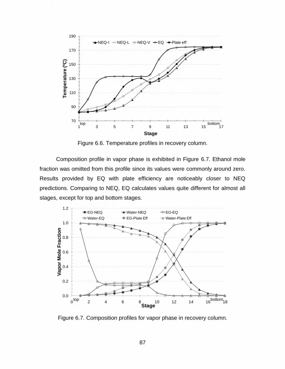
87

Figure 6.6. Temperature profiles in recovery column.

Composition profile in vapor phase is exhibited in Figure 6.7. Ethanol mole

fraction was omitted from this profile since its values were commonly around zero.

Results provided by EQ with plate efficiency are noticeably closer to NEQ

predictions. Comparing to NEQ, EQ calculates values quite different for almost all

stages, except for top and bottom stages.

Figure 6.7. Composition profiles for vapor phase in recovery column.

70

90

110

130

150

170

190

1 3 5 7 9 11 13 15 17

Te

mp

era

ture

(ºC

)

Stage

NEQ-I NEQ-L NEQ-V EQ Plate eff

top bottom

0.0

0.2

0.4

0.6

0.8

1.0

1.2

0 2 4 6 8 10 12 14 16 18

Va

po

r M

ole

Fra

cti

on

Stage

EG-NEQ Water-NEQ EG-EQ

Water-EQ EG-Plate Eff Water-Plate Eff

top bottom

88

CONCLUDING REMARKS

Extractive distillation process consists of an extractive distillation and a

conventional distillation column that is responsible for solvent recovery. In this

work, Barros and Wolf efficiency correlations for plate and component developed

for these two processes were evaluated through comparison to nonequilibrium

stage model. Results showed that the addition of plate efficiencies improved the

predictions of equilibrium stage model. However, the consideration of component

efficiencies did not seem to be accurate.

Temperature profiles showed that temperatures of vapor phase differ from

those of interface and liquid phase; hence vapor phase controls the heat transfer in

the process. Besides, it confirms that the assumption of equal temperatures for

both phases, as stated in EQ, is not reasonable.

In summary, this study reconciles efficiency correlations and equilibrium

stage model calculations performed by the commercially available software Aspen

Plus®. Although this software also comprises a nonequilibrium stage model, it

requires the knowledge of some design properties; additionally, computational time

for nonequilibrium stage model calculations is significantly high as well as its

complexity, leading to convergence problems, which are not desirable in online

control applications. The use of efficiency correlation has the objective of simplify

the calculations when compared to NEQ and, at the same time, increase accuracy

of predictions in comparison to the idealized equilibrium stage model.


Este capítulo apresentou o processo de destilação extrativa, incluindo a

coluna de destilação extrativa e a coluna de destilação convencional empregada

na recuperação de solvente.

A aplicação das correlações de eficiência de Barros e Wolf para prato e

componente foi avaliada através da comparação com os resultados preditos pelo

modelo de estágios de não equilíbrio. A incorporação de eficiências de prato

aumentou a acurácia da predição do modelo de estágio de equilíbrio, enquanto as

89

simulações considerando as eficiências de componente não apresentaram

resultados satisfatórios.

Observou-se ainda que as simulações utilizando a modelagem de não

equilíbrio requerem o conhecimento de alguns dados de projeto, além de maior

tempo para a realização dos cálculos. A complexidade deste modelo assim como

aumenta a acurácia das predições também induz a problemas de convergência,

dessa forma não é aconselhável para aplicações em controle online.

90

Capítulo 7

Simulação do Processo de Produção de Bioetanol

usando Correlações de Eficiência para Destilação

Convencional e Extrativa

7.1. Introdução

Assim como apresentado nos capítulos anteriores, a simulação das etapas

de concentração e desidratação é de grande importância no processo de

produção de bioetanol. Para essas etapas, foram avaliadas as correlações de

eficiência de Barros e Wolf para as destilações convencional e extrativa.

Neste capítulo, as etapas de concentração e desidratação são analisadas

em conjunto para avaliar o efeito da introdução da eficiência de prato nos cálculos

da modelagem de estágios de equilíbrio.


intitulado “Simulation of Anhydrous Bioethanol Production Process using Efficiency

Correlations for Conventional and Extractive Distillation” submetido ao 9th

Distillation & Absorption Conference - DA 2010.

7.2. Simulation of Anhydrous Bioethanol Production Process

using Efficiency Correlations for Conventional and Extractive

Distillation

ABSTRACT

In this work, simulations of the complete separation process in anhydrous

bioethanol production were carried out in Aspen Plus®. This process comprises

distillation and rectification columns as well as an extractive column. Equilibrium

stage model and Barros & Wolf efficiency correlations were used to perform the

calculations. Efficiency profiles were obtained for all columns showing that

efficiency values significantly vary along the columns. Influence of the introduction

of efficiencies was evaluated through comparison with equilibrium stage model

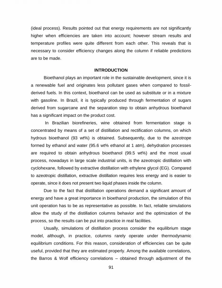
91

(ideal process). Results pointed out that energy requirements are not significantly

higher when efficiencies are taken into account; however stream results and

temperature profiles were quite different from each other. This reveals that is

necessary to consider efficiency changes along the column if reliable predictions

are to be made.

INTRODUCTION

Bioethanol plays an important role in the sustainable development, since it is

a renewable fuel and originates less pollutant gases when compared to fossil-

derived fuels. In this context, bioethanol can be used as substitute or in a mixture

with gasoline. In Brazil, it is typically produced through fermentation of sugars

derived from sugarcane and the separation step to obtain anhydrous bioethanol

has a significant impact on the product cost.

In Brazilian biorefineries, wine obtained from fermentation stage is

concentrated by means of a set of distillation and rectification columns, on which

hydrous bioethanol (93 wt%) is obtained. Subsequently, due to the azeotrope

formed by ethanol and water (95.6 wt% ethanol at 1 atm), dehydration processes

are required to obtain anhydrous bioethanol (99.5 wt%) and the most usual

process, nowadays in large scale industrial units, is the azeotropic distillation with

cyclohexane, followed by extractive distillation with ethylene glycol (EG). Compared

to azeotropic distillation, extractive distillation requires less energy and is easier to

operate, since it does not present two liquid phases inside the column.

Due to the fact that distillation operations demand a significant amount of

energy and have a great importance in bioethanol production, the simulation of this

unit operation has to be as representative as possible. In fact, reliable simulations

allow the study of the distillation columns behavior and the optimization of the

process, so the results can be put into practice in real facilities.

Usually, simulations of distillation process consider the equilibrium stage

model, although, in practice, columns rarely operate under thermodynamic

equilibrium conditions. For this reason, consideration of efficiencies can be quite

useful, provided that they are estimated properly. Among the available correlations,

the Barros & Wolf efficiency correlations – obtained through adjustment of the

92

mixture properties, such as thermal conductivity, density, heat capacity and

diffusivity – can be used to calculate efficiencies for conventional and extractive

distillations (Reis et al., 2006; Wolf-Maciel et al., 2001).

In this work, simulations of the complete separation process for bioethanol

production was carried out in Aspen Plus® considering the equilibrium stage model

and the efficiency values obtained through Barros & Wolf efficiency correlations.

The purpose of this work is to analyze the influence of incorporating efficiency in

the column calculations.

PROCESS DESCRIPTION

Hydrous Bioethanol Production

In order to produce hydrous bioethanol, most Brazilian biorefineries employ the

configuration depicted in Figure 7.1, which consists of a series of distillation and

rectification columns. Initially, the wine produced in the fermentation stage is fed to

column A1 originating the top and bottom products that are sent to column D and

A, respectively. Column D is responsible for removing volatile contaminants at the

top, whereas column A removes large amounts of water (stillage or vinasse) in the

bottom. Vapor phlegm produced near to the top of column A and liquid phlegm

obtained at the bottom of column D are sent to rectification columns (column B-

B1). The task of the rectification section is to concentrate the phlegm streams from

40-50 wt% to 93 wt% ethanol (hydrous bioethanol, “HE”). Sidestreams are

withdrawn from column B-B1 and correspond to fusel oil, which is mainly

characterized by isoamyl alcohol presence.


93

Anhydrous Bioethanol Production

In this work, the extractive distillation process was considered as the method

to separate the azeotropic mixture in order to produce anhydrous bioethanol.

Extractive distillation, also known as homogeneous azeotropic distillation, is

commonly used to separate nonideal mixtures with close boiling point or

azeotropes. In this process, a heavy boiling solvent is added to the system to be

separated, which alters the volatility of the component in the original mixture. Care

has to be taken in the choice of the solvent since new azeotropes must not be

formed and the solvent must be completely miscible in the mixture, in other words,

it must not form a second liquid phase as in heterogeneous azeotropic distillation

(Reis et al., 2006; Dias et al., 2009a). The conventional configuration employed in

bioethanol production process is shown in Figure 7.2.

Figure 7.2. Configuration of extractive distillation process.

As can be seen in Figure 7.2, solvent is fed to the first column (extractive

column, “EC”), above the azeotropic feed. Anhydrous ethanol is produced on the

top of the extractive column, while in the bottom a mixture containing solvent and

water is obtained. The solvent is recovered in a second column (recovery column,

“RC”), which is operated under vacuum (0.5 bar), then cooled and recycled to the

first column.

94

EFFICIENCY CORRELATIONS

Several works have shown the deviations of the equilibrium stage model

results from experimental data (Springer et al., 2002; Repke et al., 2004; Nava and

Krishna, 2004). In order to correct this weakness, efficiency can be introduced in the

equilibrium calculations.

For instance, efficiency correlations were developed by Barros (1997) based

on techniques of factorial design. These correlations, known as Barros & Wolf

efficiency correlations, were proposed for conventional (Equation 7.1) and extractive

(Equation 7.2) distillations.

04516.0

2 )i()i(Cp

)i(MW)i(D)i()i(k5309.38)i(Eff (7.1)

109588.0

2 )i()i(Cp

)i(MW)i(D)i()i(k37272.19)i(Eff (7.2)

In Equations 7.1 and 7.2, Eff (i) is the plate efficiency, which is a function of

the following properties of the mixture: thermal conductivity (k), density ( ),

diffusivity (D), molecular weight (MW), heat capacity (Cp) and viscosity ( ).

Wolf-Maciel and collaborators (2001) evaluated the performance of the

Barros & Wolf efficiency correlation for a conventional distillation column using

ethanol-water system. Comparison with nonequilibrium stage model and

experimental data were carried out and a satisfactory agreement was achieved,

validating the use of Barros & Wolf efficiency correlation. Similarly, Reis and

coauthors (2006) validated Barros & Wolf efficiency correlation for extractive

distillation columns.

SIMULATION PROCEDURE

For calculations, NRTL model was used for the estimation of activity

coefficients and vapor phase was considered ideal, since previous work about

thermodynamic characterization has showed the adequacy of this model.

Typical industrial compositions of wine and hydrous bioethanol were

considered the same for both approaches and are shown in Table 7.1. Additionally,

95

configurations of the conventional and extractive distillation processes used in the

simulations are those depicted in Figures 7.1 and 7.2, respectively. Column

specifications are given in Table 7.2 and 7.3. Stages numbering initiates from the

top stage or condenser, when it is present and coupled reboiler is considered the

last stage.

Correlation for conventional columns (Equation 7.1) was used to determine

plate efficiency in the rectification and distillation columns employed in the

concentration of wine and in the solvent recovery column, whereas correlation for

extractive distillation (Equation 7.2) was used only for the ethanol dehydration

column. Condenser and reboiler were considered as equilibrium stages for both

calculation approaches.

The procedure to determine and include efficiencies in the calculation

procedure was an iterative method. First, simulations considering equilibrium stage

model were carried out in Aspen Plus® without the addition of efficiency values, which

means an efficiency of 100 % (ideal situation). Subsequently, mixture properties were

retrieved from the previous simulation and used to calculate the initial values of

efficiency through Barros & Wolf efficiency correlation. These efficiencies were

inserted in the simulation as Murphree efficiencies and the properties were

recalculated, thus obtaining new efficiencies values. This procedure was repeated

until the difference between two consecutive efficiency iterations reached a level of

tolerance below 1.10-4.

Table 7.1. Composition of the streams fed to the process.

Wine Hydrous bioethanol

Water (wt%) 92.0 7.0

Ethanol (wt%) 7.3 93.0

Glycerol (wt%) 0.4 -

Isoamyl alcohol (wt%) 0.2 -

Glucose (wt%) 0.1 -

Mass Flow (t/h) 207.0 16.1

96

Table 7.2. Column specifications in bioethanol production process.

Column A Column A1 Column D Column B-B1

Number of stages 19 8 6 46

Feed stage 1 1 (WINE)

8 (TOP-A)

1 (REFLUX)

6 (TOP-A1)

22 (PHLEGM-L)

22 (PHLEGM-V)

Sidestream rate (kg/h)

PHLEGM-V 30000 (2V)

- - 500 (FUSEL1 - 21L)

300 (FUSEL2 - 45L)

Distillate rate (kg/h) 12750 16100

Number in parenthesis shows the withdrawal stage. Superscript denotes the phase, L for

liquid and V for vapor.

Table 7.3 Specifications in the extractive and recovery columns (mass basis).

Extractive Column Recovery Column

Number of Stages 32 18

Feed Position 3 (SOLVENT) and 24 (HE) 9

Solvent to Feed Ratio 0.62 -

Reflux Ratio 1.05 0.38

Distillate Rate (kg/h) 15051 -

Bottoms Rate (kg/h) - 9984.0


Efficiency profiles were generated for all columns employed in the complete

process and can be seen in Figure 7.3. It was observed quite different profile for

each column. Generally, efficiencies were around 50 % and varied along the

columns, except for column A1, which presented constant values.

Figure 7.3. Efficiency profiles obtained in the columns.

45

47

49

51

53

55

0 5 10 15 20 25 30 35 40 45 50

Eff

icie

ncy

(%

)

Stage

Column A Column A1

Column B-B1 Column D

bottomtop

97

Results of main streams are compared through Tables 7.4 and 7.5. It can be

inferred that ethanol contents in hydrous ethanol (HE) and in anhydrous ethanol

(AE) are lower when efficiency is taken into account; moreover there is ethanol

loss in phlegmasse (PHLEGMAS) and water streams. Stillage and solvent results

were the same for both approaches.

Table 7.4. Stream results for hydrous bioethanol production.

Equilibrium Stage Model (Ideal) Equilibrium Stage Model with Efficiency

STILLAGE PHLEGMAS HE STILLAGE PHLEGMAS HE

Temperature (°C) 111.9 107.0 81.7 111.9 105.6 81.7

Mass Flow (kg/h) 175418 14622 16100 175240 14800 16100

Water (wt%) 99.4 99.4 6.8 99.4 98.6 7.6

Glucose (wt%) 0.1 - - 0.1 - -

Ethanol (wt%) - - 93.2 - 0.1 92.4

Glycerol (wt%) 0.5 - - 0.5 - -

Isoamyl alcohol (wt%) - 0.6 - - 1.3 -

Table 7.5 Stream results for anhydrous bioethanol production.

Equilibrium Stage Model (Ideal) Equilibrium Stage Model with Efficiency

AE SOLVENT WATER AE SOLVENT WATER

Temperature (°C) 78.3 110 83.5 78.4 110 82.0

Pressure (bar) 1.013 1.013 0.5 1.0 1.0 0.5

Mass Flow (kg/h) 15051 9989 1054 15051 9989.0 1054.0

Ethanol (wt%) 99.5 - - 99.4 - 1.3

Water (wt%) 0.5 - 99.6 0.6 - 98.5

Ethylene glycol (wt%) - 100 0.4 - 100 0.1

Comparison of temperature profiles in column B-B1 is illustrated in Figure

7.4. This column was chosen since it has a larger number of stages and, as a

result, it is the most influenced column in this process, concerned with the

objectives of this work. It was observed that the curves significantly detach from

each other between stages 11 and 31, besides the fact that equilibrium stage

model (EQ) presents the highest temperature values. This fact can be explained by

the assumption that there is enough contact time between the phases to achieve

thermal equilibrium. Another observation is that EQ is more sensible to column

operation, since the profile presents a disturbance in the feed position (stage 22).

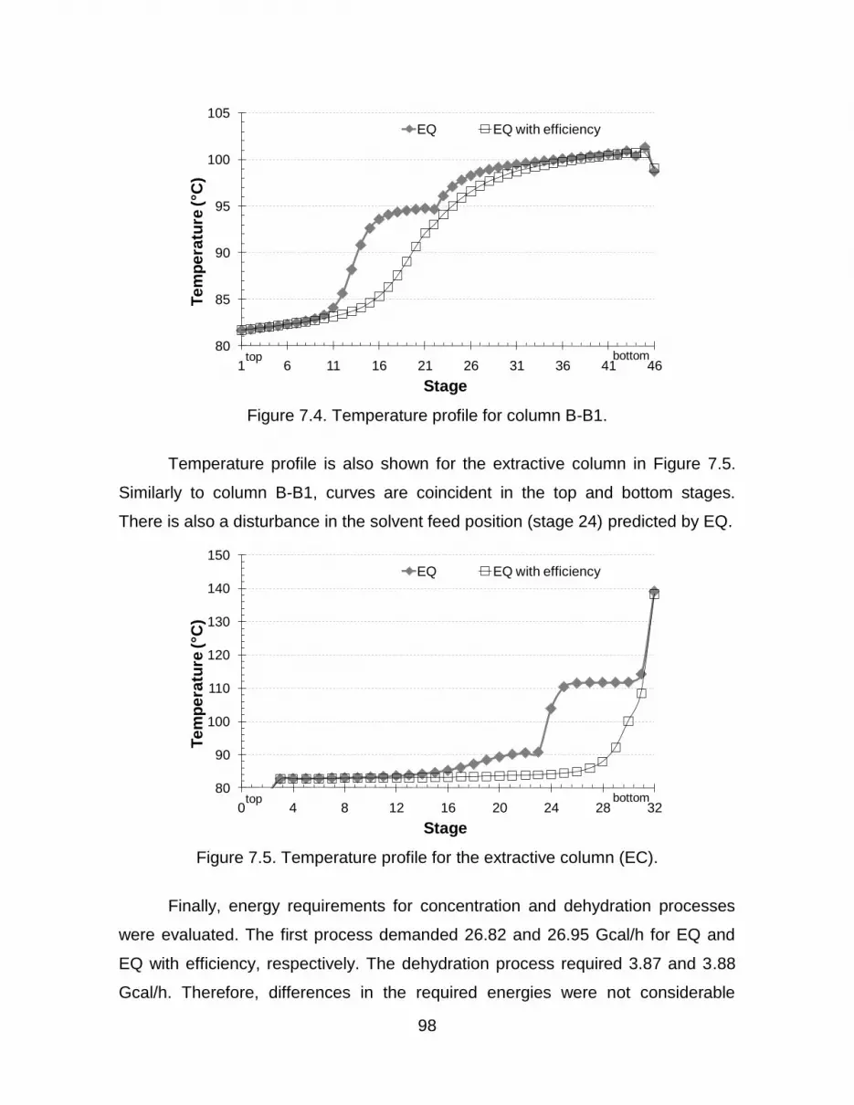
98

Figure 7.4. Temperature profile for column B-B1.

Temperature profile is also shown for the extractive column in Figure 7.5.

Similarly to column B-B1, curves are coincident in the top and bottom stages.

There is also a disturbance in the solvent feed position (stage 24) predicted by EQ.

Figure 7.5. Temperature profile for the extractive column (EC).

Finally, energy requirements for concentration and dehydration processes

were evaluated. The first process demanded 26.82 and 26.95 Gcal/h for EQ and

EQ with efficiency, respectively. The dehydration process required 3.87 and 3.88

Gcal/h. Therefore, differences in the required energies were not considerable

80

85

90

95

100

105

1 6 11 16 21 26 31 36 41 46

Te

mp

era

ture

(°C

)

Stage

EQ EQ with efficiency

top bottom

80

90

100

110

120

130

140

150

0 4 8 12 16 20 24 28 32

Te

mp

era

ture

(°C

)

Stage

EQ EQ with efficiency

top bottom

99

between the calculation methods. However, energy requirements in the

concentration process revealed to be significantly higher than in dehydration.

Larger flows are the main responsible for this difference.

CONCLUSIONS

This work has shown the complete separation process in the anhydrous

bioethanol production. This is an important step in the product production with a

significant impact on the costs. Contrasting to other published works, this study

considered other components in wine composition as well as all columns included

in the process. Solvent recovery column is usually disregarded and concentration

process is usually simplified using a single column. Therefore, simulations were

more complex and detailed so that a more deep study can be carried out.

The introduction of efficiencies is important to diminish the consequences of

the idealized assumptions of equilibrium stage model. In the simulated process,

efficiencies varied along the columns, oscillating around 50 %.

Results showed significant differences in respect to stream results and

temperature profiles, although energy requirements were not so influenced by the

inclusion of efficiency. The concentration process revealed to be the main

responsible for energy demand in the anhydrous bioethanol production process,

particularly due to the large flows involved.


Neste capítulo, o processo de separação completo empregado na produção

de bioetanol anidro foi simulado. Diferentemente de outros trabalhos publicados,

este estudo considerou co-produtos da fermentação na composição do vinho. A

configuração composta por um conjunto de colunas de retificação e destilação

usualmente empregada nas biorrefinarias foi considerada bem como o processo

de destilação extrativa completo, ou seja, incluindo também a coluna de

recuperação de solvente.

Nos processos baseados em destilação, tem-se que a introdução de

eficiências diminui as implicações da suposição de equilíbrio entre as fases líquida

100

e vapor que deixam cada estágio. Para todo o processo de separação, os valores

de eficiência variaram ao longo das colunas, no entanto, permaneceram em torno

de 50 %.

A comparação entre os resultados da modelagem de equilíbrio sem e com a

introdução de eficiência revelou diferenças significativas no que se refere à

composição e condições das correntes de saída e aos perfis de temperatura,

entretanto o consumo de energia nos refervedores das colunas não apresentou

diferença significativa com a inclusão das eficiências.

Comparando-se a demanda de energia nas etapas de concentração e

desidratação do bioetanol, tem-se que a etapa de concentração requer mais

energia, principalmente por envolver correntes de processo com maiores vazões.

101

Capítulo 8

Simulação da Destilação Azeotrópica no Processo de

Produção de Bioetanol Anidro

8.1. Introdução

Sendo o processo de desidratação mais utilizado nas biorrefinarias

brasileiras, a destilação azeotrópica com cicloexano é caracterizada pelo alto

consumo de vapor de processo e pela complexidade de operação decorrente da

formação de duas fases líquidas no interior da coluna.

A formação de duas fases líquidas na coluna de destilação influencia a

transferência de massa do processo, afetando a eficiência deste (Higler et al.,

2004). Neste capítulo, o processo de destilação azeotrópica foi simulado através

do software Aspen Plus® utilizando a modelagem de estágios de equilíbrio. A

formação de duas fases líquidas no interior da coluna azeotrópica foi analisada e,

com o intuito de diminuir esse fenômeno, foram estudadas diferentes

configurações de processo bem como variações nas condições de operação.

Considerou-se que a alimentação do processo é bioetanol hidratado com a

mesma composição indicada na seção 5.2. O objetivo da simulação foi a produção

de bioetanol anidro (99,5 % em massa).

O desenvolvimento deste capítulo é descrito a seguir no trabalho intitulado

“Simulation of the azeotropic distillation for anhydrous bioethanol production: study

on the formation of a second liquid phase”, publicado no periódico Computer Aided

Chemical Engineering, v. 27, p. 1143-1148 (2009), decorrente da participação no

10th International Symposium on Process Systems Engineering (PSE’09).

102

8.2. Simulation of the azeotropic distillation for anhydrous

bioethanol production: study on the formation of a second liquid

phase

ABSTRACT

Bioethanol is produced from fermentation of sugars, what produces a dilute

solution (around 10 wt% ethanol). Because water and ethanol form an azeotrope

with concentration of 95.6 wt% ethanol at 1 atm, an alternative separation process

such as azeotropic distillation must be employed to produce anhydrous bioethanol,

which can be used in a mixture with gasoline. In this work, simulations of three

different configurations of the azeotropic distillation process with cyclohexane for

anhydrous bioethanol production were carried out using software Aspen Plus.

Process parameters were optimized in order to decrease the formation of a second

liquid phase inside the column. Ethanol and entrainer losses as well as energy

demand were evaluated.

INTRODUCTION

Climate change and the consequent need to diminish greenhouse gases

emissions have encouraged the use of bioethanol in a mixture with or as a

replacement of gasoline. In order to be used in a mixture with gasoline, ethanol

produced from fermentation of sugars, obtained at a concentration of about 10 wt%

ethanol, must be concentrated to at least 99.3 %. Since ethanol and water form an

azeotrope with 95.6 wt% ethanol at 1 atm, conventional distillation can not achieve

the necessary separation that meets product specification. The main processes

employed for anhydrous bioethanol production are azeotropic and extractive

distillation and adsorption on molecular sieves.

In the conventional configuration of the heterogeneous azeotropic distillation

process for anhydrous bioethanol production, two distillation columns are used: the

azeotropic one and the recovery unit. Hydrous ethanol and entrainer are fed in the

azeotropic column, where anhydrous ethanol is produced on the bottom and a

minimum boiling ternary azeotrope formed between ethanol, water and entrainer is

produced on the top. The ternary azeotrope is heterogeneous, and the two liquid

103

phases are separated in a decanter. The light phase contains most of the entrainer

and is recycled to the azeotropic column, while the aqueous phase is fed to the

recovery column where ethanol and eventually entrainer are recovered. The

stream containing ethanol recovered may be recycled to the azeotropic column, in

order to reduce ethanol losses.

Benzene was the most common entrainer employed in anhydrous

bioethanol production, but due to its carcinogenic characteristics cyclohexane is

most frequently used nowadays. The azeotropic distillation process with

cyclohexane is the most common method for anhydrous bioethanol production

employed in Brazil, which is the second largest ethanol producer in the world. This

process is characterized by high steam consumption on column reboilers, as well

as high entrainer losses on the product. In other words, the separation step for

obtaining anhydrous ethanol has a significant impact on the final product price, so

that it is worthwhile to investigate procedures and alternatives to improve the

process economy and performance. Simulation is an attractive tool to evaluate the

process since it is not suitable to use large scale units to do so.

Simulation of the azeotropic distillation process is often complex and

extremely sensitive to project parameters and specifications, mainly because of the

formation of a second liquid phase inside the azeotropic column, which influences

the mass transfer behaviour: column efficiencies between 25 and 50 % are not

uncommon when a second liquid phase is present (Higler et al., 2004).

In this work simulations of the azeotropic distillation process with

cyclohexane for anhydrous bioethanol production were carried out using software

Aspen Plus. Simulation of different process configurations were carried out, and

the main parameters evaluated were the formation of the second liquid phase

inside the column, the separation of the ternary azeotrope during settling, entrainer

losses on the anhydrous bioethanol and energy consumption on column reboilers.

Heterogeneous azeotropic distillation

Heterogeneous azeotropic distillation is widely employed in industry as a

separation process for azeotropic or close-boiling mixtures, for which conventional

distillation can not achieve the necessary separation. In this process, a third

104

component, called entrainer, is added to the binary mixture, producing a

heterogeneous azeotrope with one or both components of the original mixture. In

the separation of a binary azeotropic mixture, the new azeotrope produces a more

favorable azeotropic pattern for the desired separation. Even though the formation

of a second liquid phase simplifies entrainer recovery and the recycle process, it

may affect column performance and, consequently, decrease efficiency. Different

process configurations can lead to a decreased formation of a second liquid phase,

without compromising anhydrous bioethanol production.

Simulation of the azeotropic distillation process

Three different configurations of the azeotropic distillation process with

cyclohexane for anhydrous bioethanol production were simulated using software

Aspen Plus. NRTL was the model used for calculation of the activity coefficient on

the liquid phase. Approximately 500 m3/day of anhydrous bioethanol (99.5 wt%

ethanol) are produced on each case, from 16,100 kg/h (521 m3/day) of hydrous

bioethanol (93 wt% ethanol).

Configuration 1

The first configuration of the process is depicted in Figure 8.1. In this case,

hydrous bioethanol is mixed with the recycle stream of the recovery column and

fed to the azeotropic column. Entrainer is comprised by the organic phase obtained

in the decanter and a solvent make-up stream. Anhydrous bioethanol is produced

on the bottom of the azeotropic column, and the ternary azeotrope in the top. After

cooling, the ternary azeotrope splits into two liquid phases in the decanter. The

aqueous phase is fed to the recovery column, producing pure water on the bottom.

Figure 8.1. First configuration of the azeotropic distillation process.

105

Configuration 2

The main difference between this configuration and the first one is the

withdrawn of a fraction of the aqueous phase obtained in the decanter and its

mixture with the hydrous ethanol and recycle stream, which are fed to the

azeotropic column (Mortaheb and Kosuge, 2004). Configuration 2 of the azeotropic

distillation process is displayed in Figure 8.2.

Figure 8.2. Second configuration of the azeotropic distillation process.

Configuration 3

In the third configuration part of the ternary azeotrope is condensed and

mixed with hydrous ethanol, being subsequently fed to the azeotropic column. In

this configuration the top product of the recovery column is not recycled to the

azeotropic column, but to the decanter. This configuration is depicted in Figure 8.3.

Figure 8.3. Third configuration of the azeotropic distillation process.

106

Simulation parameters

Columns parameters are displayed in Table 8.1. Stage numbering initiates in the

top stage or attached condenser and reboiler is considered the last stage.

Table 8.1. Process parameters for each configuration.

Configuration 1 Configuration 2 Configuration 3

COL-AZ number of stages 31 31 31

Feed inlet stage – COL-AZ 18 20 20

Solvent inlet stage 1 1 1

COL-REC number of stages 25 22 17

Feed inlet stage – COL-REC 13 13 13

Decanter temperature (°C) 50 50 50

Simulation results and discussion

Main streams results

The characteristics of process stream differ for each configuration. Results

are presented in Tables 8.2 through 8.4.

Table 8.2. Composition of the main streams for the first configuration.

Stream AE MAKE-UP ORG AQUEOUS WATER

Temperature (ºC) 78.2 50.0 50.0 50.0 100.0

Flow (kg/h) 15063.6 16.8 42501.6 19524.1 1053.5

Ethanol (wt%) 99.5 0.0 4.7 71.2 0.0

Water (wt%) 0.4 0.0 0.1 10.8 100.0

Cyclohexane (wt%) 0.1 100.0 95.2 18.0 0.0

Table 8.3. Composition of the main streams for the second configuration.


Temperature (ºC) 78.2 50.0 50.0 50.0 100.0

Flow (kg/h) 15064.4 21.0 50274.1 22813.3 1057.3

Ethanol (wt%) 99.5 0.0 4.6 71.5 0.0

Water (wt%) 0.4 0.0 0.1 11.3 100.0

Cyclohexane (wt%) 0.1 100.0 95.3 17.2 0.0

107

Table 8.4. Composition of the main streams for the third configuration.


Temperature (ºC) 78.1 50.0 50.0 50.0 78.6

Flow (kg/h) 8395.4 16.8 22877.5 31880.6 7722.0

Ethanol (wt%) 99.5 0.0 5.2 67.6 85.9

Water (wt%) 0.3 0.0 0.1 7.5 14.1

Cyclohexane (wt%) 0.2 100.0 94.7 24.9 0.0

Streams obtained in the decanter (AQUEOUS and ORG) have different

compositions on each studied configuration. Configurations 1 and 2 showed similar

results, while configuration 3 had a higher concentration of solvent in the aqueous

phase. Due to this contamination, recovery column behaviour was significantly

affected and “WATER” stream has a high concentration of ethanol (85.9 wt%), so it

must be recycled to the previous distillation stage, where hydrous bioethanol is

produced.

Energy consumption and entrainer and ethanol losses

Different process parameters affect ethanol and entrainer losses, as well as

energy consumption on column reboilers. The results for these parameters are

given in Table 8.5.

Table 8.5. Ethanol and entrainer losses and energy consumption on column

reboilers for each configuration.

Configuration 1 Configuration 2 Configuration 3

Ethanol losses (%)* 0.00 0.00 44.26

Entrainer losses (%)** 0.04 0.03 0.07

Reboilers energy (kJ/kg AE) 5588 5828 7235

* Considering the amount of ethanol in the “HE” stream

** Considering the amount of cyclohexane that is fed to the azeotropic column

The “WATER” stream on the third configuration has a very high

concentration of ethanol, thus ethanol losses on this configuration are significant.

The recycle of this stream to the conventional distillation column would allow

ethanol recovery at the expense of an increase in energy consumption of the

process, which already has the largest energy consumption on column reboilers.

108

Configurations 1 and 2, on the other hand, present low ethanol and entrainer

losses, as well as a relatively low energy consumption.

Formation of the second liquid phase inside the azeotropic column

Similar liquid flow profiles were observed in the azeotropic column. The

profiles for each configuration are represented in Figures 8.4 through 8.6.

Figure 8.4. Liquid flow profile in the azeotropic column for configuration 1.

Changes in column parameters, such as feed inlet position in the azeotropic

column, greatly influence the formation of a second liquid phase. For the first

configuration, the feed inlet stage in the azeotropic column (18) is the one that first

presents two liquid phases. The same occurs for the other configurations. The feed

inlet stage is the last one that allows column convergence; on the other hand, if the

feed stage is located near the top of the column, two liquid phases are present in

this region too. This means that the feed inlet stage in the azeotropic column has to

be defined with caution, since it impacts unit behavior and performance.


Stage

Flo

w (

t/h

)

1.0 6.0 11.0 16.0 21.0 26.0 31.0

20

.040

.060

.080

.010

0.0 1st Liquid Flow

2nd Liquid Flow

Stage

Flo

w (

t/h

)

1.0 6.0 11.0 16.0 21.0 26.0 31.0

20

.040

.060

.080

.010

0.0

1st Liquid Flow

2nd Liquid Flow

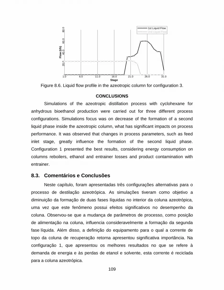
109


CONCLUSIONS

Simulations of the azeotropic distillation process with cyclohexane for

anhydrous bioethanol production were carried out for three different process

configurations. Simulations focus was on decrease of the formation of a second

liquid phase inside the azeotropic column, what has significant impacts on process

performance. It was observed that changes in process parameters, such as feed

inlet stage, greatly influence the formation of the second liquid phase.

Configuration 1 presented the best results, considering energy consumption on

columns reboilers, ethanol and entrainer losses and product contamination with

entrainer.


Neste capítulo, foram apresentadas três configurações alternativas para o

processo de destilação azeotrópica. As simulações tiveram como objetivo a

diminuição da formação de duas fases líquidas no interior da coluna azeotrópica,

uma vez que este fenômeno possui efeitos significativos no desempenho da

coluna. Observou-se que a mudança de parâmetros de processo, como posição

de alimentação na coluna, influencia consideravelmente a formação da segunda

fase líquida. Além disso, a definição do equipamento para o qual a corrente de

topo da coluna de recuperação retorna apresentou significativa importância. Na

configuração 1, que apresentou os melhores resultados no que se refere à

demanda de energia e às perdas de etanol e solvente, esta corrente é reciclada

para a coluna azeotrópica.

Stage

Flo

w (

t/h

)

1.0 6.0 11.0 16.0 21.0 26.0 31.0

20

.040

.060

.080

.0 1st Liquid Flow

2nd Liquid Flow

110

Capítulo 9

Simulação do Processo de Extração Fermentativa a

Vácuo e Análise do Impacto na Etapa de Destilação

9.1. Introdução

Como mostrado na seção 3.2, como alternativa para o processo

fermentativo, Silva et al. (1999) e Atala (2004) estudaram a fermentação extrativa

a vácuo, que consiste em um processo fermentativo contínuo acoplado a um

evaporador a vácuo do tipo flash. Esta configuração permite que uma maior

quantidade de substrato seja adicionada ao reator, produzindo um vinho mais

concentrado. Consequentemente, a destilação deste vinho produz menores

volumes de resíduos como a vinhaça. Adicionalmente, tem-se a diminuição da

demanda de energia térmica do processo de destilação.

Neste capítulo, esta configuração alternativa em conjunto com a destilação

foi estudada a fim de se avaliar o processo, principalmente quanto à energia

requerida. Outra alteração do processo foi a realização da integração energética

no processo de destilação (destilação duplo e triplo efeito).

O desenvolvimento deste capítulo é apresentado a seguir, no trabalho

intitulado “Evaluation of an extractive fermentation process coupled with a vacuum

flash chamber and the subsequent distillation for bioethanol production” a ser

submetido a periódico internacional.

9.2. Evaluation of an extractive fermentation process coupled

with a vacuum flash chamber and the subsequent distillation for

bioethanol production

ABSTRACT

An alternative to the conventional fed-batch fermentation process for bioethanol

production, the extractive fermentation process coupled with a vacuum flash

chamber, is evaluated in this work through process simulation. In the alternative

process, ethanol produced is continuously removed from the fermentation medium,

111

thus decreasing inhibitory effects on yeast cells and producing a wine of higher

ethanol content, which leads to decreased energy consumption and residue

generation on the subsequent distillation step, where wine purification takes place.

Different configurations of the distillation system (conventional, double and triple

effect) for hydrous bioethanol (93 wt%) production are integrated to the studied

fermentation process, providing resources that allow the comparison of different

process configurations and their impacts on bioethanol losses, energy

consumption and residue generation.

INTRODUCTION

The efficient production of renewable fuels is one of the most significant

challenges faced by humanity, in a scenario of predicted depletion of fossil

resources, increase on energy demand and climate change (Dodić et al., 2009;

Saxena, 2009). Bioethanol has been acknowledged as the best viable alternative

to fossil fuels in the immediate future (Walter et al., 2008), offering environmental

and long-term economic advantages over fossil fuels (Cheng and Wang, 2008).

Even though bioethanol has been produced in a large scale basis in countries like

Brazil for more than twenty years, process improvements are still possible.

Considering the entire bioethanol production process from sugarcane, the

fermentation step, on which sugars are converted into ethanol by yeasts, is

responsible for the majority of the sugar losses: yeast cells are inhibited by product

(ethanol), substrate (sugars) and biomass (yeast cells), and fermentation yields are

limited due to cells growth, rising temperature (Rivera et al., 2006) and byproducts

formation during parallel fermentation reactions (Bai et al., 2008). One of the main

alternatives to increase fermentation yields by minimizing inhibition by product is

the removal of ethanol from fermentation media, based on vacuum fermentation

(Ramalingham and Finn, 1977; Cysewski and Wilke, 1978), on pervaporation

techniques (Christen et al., 1990; Thongsukmak and Sirkar, 2009), on liquid-liquid

extraction (Daugulis et al., 1991; Chen and Wang, 2008) and on the integration of

a flash to the process (Ishida and Shimizu, 1996; Maiorella et al., 1984; Silva et al.,

1999; Costa et al., 2001). The fermentation system coupled with a vacuum flash

chamber seems to be the most adequate process for industrial application in

112

Brazil, due to its ease of operation and low cost (Silva et al., 1999). In this process,

ethanol is continuously removed from the fermentation media, simultaneously to its

production, allowing ethanol concentration in the reactor to remain at low levels (5

°GL), which presents low inhibitory effects on yeast cells. In addition, wine obtained

in the flash chamber presents higher ethanol concentration (around 50 °GL), what

reduces energy consumption and ethanol losses on the subsequent distillation step

(Atala, 2004). As a consequence of the reduction on energy consumption, less

sugarcane bagasse need to be burnt in boilers to provide energy to supply the

plant; thus, larger amounts of bagasse may be available for the hydrolysis process

when 2nd generation ethanol production takes place.

After fermentation is achieved, wine is concentrated on a series of distillation

and rectification columns, producing hydrous bioethanol (around 95 °GL). Since

wine produced in conventional fermentation processes contains between 7 and 10

°GL, the distillation process must be re-evaluated in order to efficiently purify the

product derived from vacuum flash fermentation.

In this work simulations of both conventional and extractive fermentation

process coupled with a vacuum flash chamber, associated with different

configurations of the subsequent distillation step were carried out using the

process simulation software Aspen Plus®. Conventional, double and triple effect

distillation systems were simulated; energy consumption, ethanol losses and

residue generation were evaluated on each case.

METHODOLOGY

Simulation of fermentation and distillation processes was carried out using

software Aspen Plus®. The Non-Random Two Liquid model for calculation of the

activity coefficient of the liquid phase and Hayden-O'Connell equation-of-state for

calculation of the vapor phase (NRTL-HOC) were employed for estimation of

thermodynamic properties. An extensive study of the thermodynamic behavior of

binary pairs present on the distillation columns for bioethanol purification was

previously carried out, and it was verified that the NRTL-HOC model represents the

system suitably.

113

In order to define the best operating conditions of the vacuum extractive

fermentation process, which allow significant reduction on energy consumption as

well as on ethanol and sugar losses, the main parameters of the flash chamber

(pressure and temperature) and the amount of wine recycled to the reactor were

carefully evaluated through several simulations. The evaluated parameters define

the phase separation in the flash chamber, and therefore the amount of ethanol

recovered in the system. This analysis is of crucial importance on the current

development stage of the technology. The results of the optimum configuration of

the extractive fermentation coupled with a flash chamber are then compared to

those obtained in the conventional fermentation process employed in the Brazilian

ethanol industry.

Different combinations between conventional and alternative (extractive

fermentation coupled with a vacuum flash chamber) fermentation processes and

conventional, double and triple effect distillation columns were carried out. A

throughout description of the studied processes is given below.

Conventional fermentation process

The simulation of the conventional fermentation process, represented in

Figure 9.1, is based on the configurations employed in the industry, on which a

substrate of relatively low concentration (around 150 g/L sucrose, which

corresponds to 15 wt% sucrose) is fed to the fermentation reactor. Fermentation

reactions are comprised by sucrose hydrolysis, producing glucose and fructose

(equation 9.1, with conversion equal to 99 %), conversion of 99.5 % of reducing

sugars into ethanol and carbon dioxide (equation 9.2) and conversion of the

remaining reducing sugars into byproducts (acetic acid and glycerol), ethanol and

carbon dioxide, as shown in equation 9.3 (Franceschin et al., 2006).

C12H22O11 + H2O → 2 C6H12O6 (9.1)

C6H12O6 →2 C2H5OH +2CO2 (9.2)

2 C6H12O6 + H2O → C2H4O2 + 2C3H8O3 + C2H5OH +2CO2 (9.3)

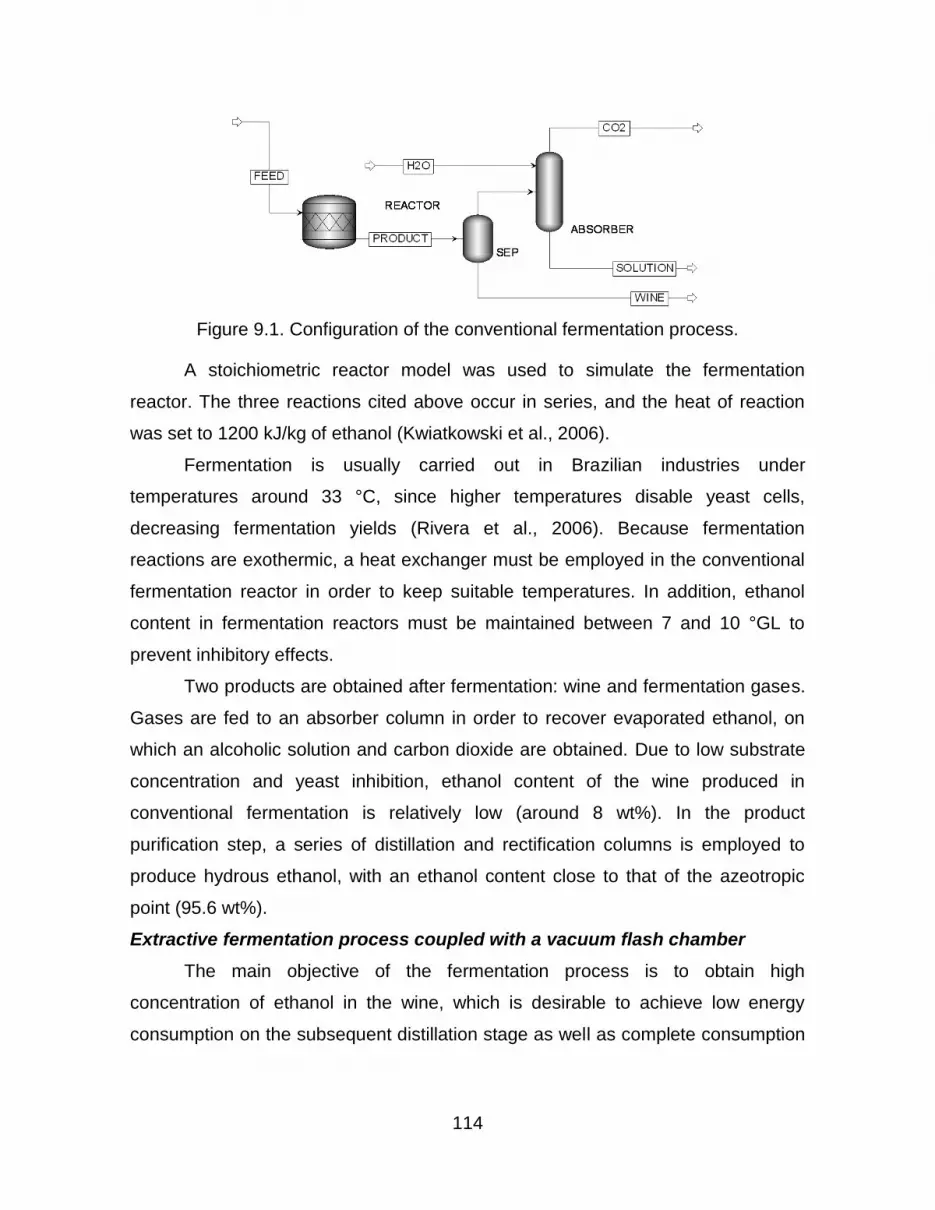
114

Figure 9.1. Configuration of the conventional fermentation process.

A stoichiometric reactor model was used to simulate the fermentation

reactor. The three reactions cited above occur in series, and the heat of reaction

was set to 1200 kJ/kg of ethanol (Kwiatkowski et al., 2006).

Fermentation is usually carried out in Brazilian industries under

temperatures around 33 °C, since higher temperatures disable yeast cells,

decreasing fermentation yields (Rivera et al., 2006). Because fermentation

reactions are exothermic, a heat exchanger must be employed in the conventional

fermentation reactor in order to keep suitable temperatures. In addition, ethanol

content in fermentation reactors must be maintained between 7 and 10 °GL to

prevent inhibitory effects.

Two products are obtained after fermentation: wine and fermentation gases.

Gases are fed to an absorber column in order to recover evaporated ethanol, on

which an alcoholic solution and carbon dioxide are obtained. Due to low substrate

concentration and yeast inhibition, ethanol content of the wine produced in

conventional fermentation is relatively low (around 8 wt%). In the product

purification step, a series of distillation and rectification columns is employed to

produce hydrous ethanol, with an ethanol content close to that of the azeotropic

point (95.6 wt%).

Extractive fermentation process coupled with a vacuum flash chamber

The main objective of the fermentation process is to obtain high

concentration of ethanol in the wine, which is desirable to achieve low energy

consumption on the subsequent distillation stage as well as complete consumption

115

of sugars in the fermentation media, but restrictions in the fermentation conditions,

such as product inhibition, must be taken into consideration.

In the extractive fermentation process coupled with a vacuum flash

chamber, ethanol produced during fermentation reactions (reactions 1, 2 and 3

cited above) is continuously removed from the fermentation media, thus allowing

the use of higher concentration substrate (around 400 g/L). The removal of

ethanol simultaneously with its production allows the ethanol content of the reactor

to remain at low levels (around 8 wt%), and so the same conversion parameters for

the conventional fermentation reactions were adopted. The product is continuously

removed from the reactor and after a purge is made to remove low-volatile

products, it is fed to a vacuum flash chamber producing an ethanol-rich vapor

phase and a liquid phase. While the vapor phase comprises the wine, which is sent

to the purification step, the liquid phase is recycled to the reactor; since the

temperature of the vacuum flash chamber is relatively low, the recycle of the liquid

stream maintains the fermentation reactor at the required temperatures (around

30 °C) without the need of external heat exchangers. Wine produced in the flash

chamber contains approximately 30 wt% ethanol, thus less energy is required to

produce hydrous ethanol and the amount of residue generated in the distillation

step is much smaller than the one produced during concentration of wine from

conventional fermentation. Configuration of the extractive fermentation process

coupled with a vacuum flash chamber is depicted in Figure 9.2.

Figure 9.2. Configuration of the vacuum extractive fermentative process.

116

Differently from the conventional fermentation process, in the vacuum

extractive fermentation process, two streams are obtained: “WINE-HC” (30 wt%

ethanol) and “WINE-LC” (8 wt% ethanol). Since the flash chamber operates under

vacuum, it is necessary to raise the pressure of the “LIGHT” stream using a series

of compressors before feeding it to the conventional distillation columns, which are

operated under atmospheric pressure. Since compression generates heat, the

compressed vapor has to be cooled, so the “PURGE” stream was used to

exchange heat with the compressed stream. In addition, the compressed stream

was used to heat up the stream that feeds the flash chamber up to around 32 °C.

Distillation

Concentration of the wine is achieved using a series of distillation and

rectification columns in order to produce hydrous bioethanol, which contains

around 93 wt% ethanol. In the conventional fermentation process, an ethanol-rich

stream (”WINE”) and an alcoholic solution from the absorber, named “SOLUTION”,

are produced. Whereas in the alternative process, two other streams are obtained:

“WINE-HC” and “WINE-LC”, comprised by flash vapour phase and a mixture of a

reactor purge. Thus, the distillation columns for each case may have different

configurations, due to the characteristics of the feed streams.

Conventional distillation

The conventional distillation system simulated in this work is based on the

configuration commonly employed in the industry: the distillation section is

comprised by three columns located in the top of each other: A (18 stages), A1 (8

stages) and D (6 stages), and rectification takes place in column B (50 stages); all

columns operate under atmospheric pressures.

In this process, the feed streams are fed to the distillation columns, on which

stillage (residue), phlegms (ethanol-rich streams, containing around 40 – 50 wt%

ethanol), second grade ethanol (a mixture with high ethanol and volatiles content)

and gases (mainly CO2) are produced; liquid phlegm is a bottom product of column

D and vapour phlegm is produced near the top of column A. Phlegms are fed to the

rectification columns, producing hydrous ethanol in the top and phlegmasse in the

117

bottom. Configuration of the conventional distillation columns is depicted in Figure

9.3. This simulation was taken as base for the alternative configurations.


When wine is produced in the extractive fermentation process, 3 compressors

must be employed in series, since the operating pressure of the flash chamber is

very low (around 0.07 bar) and that of the distillation columns is atmospheric.

When conventional fermentation is employed, no compressors are necessary.

Double effect distillation

The double effect process is similar to the conventional configuration, but

the distillation columns operate under vacuum (19 – 25 kPa), while rectification

columns operate under atmospheric pressure (101 – 135 kPa). In this way,

different temperature levels are observed between column A reboiler and column B

condenser (65 and 78 °C, respectively), allowing thermal integration of these

equipments and consequently reducing energy consumption on the distillation

stage. However, due to the low pressure of column D, large amounts of ethanol are

lost on the “GASES” stream, produced at the top of this column; thus, an absorber

was employed to recover some of the ethanol vaporized on top of column D, and a

fraction of “PHLEGMAS” stream (bottom stream of the rectification column

WINE-HC

WINE-LC

COL-A1

TOP-A1

BOT-A1

TOP-A

COL-A

STILLAGE

PHLEGM-V

COL-D

TOP-D

PHLEGM-L

COND-D FLASH2

LIQ

VAP

SPLIT2

ALCOHOL2

COL-B

ETHANOL

BOT-B

ABS

GASES

LIQUID

WATER

MIXER1

PHLEGMAS

118

containing 99.9 % of water) is used to wash the gases. Configuration of this

process applied to the alternative fermentation is depicted in Figure 9.4.

Figure 9.4. Configuration of the double effect distillation process.

Since the operating pressures of the distillation columns in this case are lower

than those of the conventional distillation, only one compressor must be used to

raise the pressure of the flash vapour phase when the extractive fermentation

process is employed. However, in the distillation step, another compressor is

necessary to raise the pressure of the top stream of column D it is sent to the

absorber column.

Triple effect distillation

In the triple effect configuration, the distillation columns operate under

vacuum (19 – 25 kPa), and the liquid phlegm stream produced on column D is split

in two: one of them is fed to a rectification column operating under nearly

atmospheric pressure (column “B”, 70 – 80 kPa) and the other is fed to a

rectification column which operates under relatively high pressure (column “B-P”,

240 – 250 kPa). As in the double effect distillation, top product of column D is

washed with phlegmasse in an absorber column in order to recover ethanol.

WINE-LC

STILLAGE

PHLEGM-V

WINE-HC

LIQUID

PHLEGM-L

ALCOHOL2

ETHANOL

WATER

GASES

PHLEGMAS

COL-A1

COL-A

COL-D

COND-D

COL-B

ABS

PUMP

HEX

COOLER

COMPR4

119

Thermal integration between columns reboilers and condensers are possible, as

depicted on Figure 9.5.

Figure 9.5. Configuration of the triple effect distillation.

RESULTS

Extractive fermentation coupled with a vacuum flash chamber

A preliminary study considering just a flash chamber was carried out. Inlet

temperature and the vessel pressure were varied in order to analyze the influence

on the outlet temperature and on the ethanol mass fraction of the vapor stream.

Results are illustrated in Figure 9.6. It can be observed that pressures below 0.05

bar result in very low temperatures, which is not desirable because the liquid

stream will be sent back to the reactor and it can reduce its temperature to less

than 28 °C. Moreover, such low pressures are very difficult and expensive to

achieve. At the same time, higher pressures lead to lower ethanol content in the

vapor phase, which will determine that of the concentrated wine (“WINE-HC”).

From Figure 9.6, it can also be verified that lower inlet temperatures result in lower

ethanol mass fractions and outlet temperatures.

WINE-LC

PHLEGM

ALCOHOL2

WINE-HC

A1

D

COND-D

A

HEX1

STILLAGE

B

HEX2

B-P

ETHANOL

ABS

GASES

PHLEGMAS

WATER

COOLER2

COOLER1

120

Figure 9.6. Analysis of the flash chamber conditions: outlet temperature of the flash

chamber and ethanol content of the flash vapor phase for different vessel

pressures.

For these reasons, further simulations considering vessel pressures of 0.05

and 0.07 bar and different inlet temperatures in the complete vacuum extractive

fermentative process, similar to the illustration depicted in Figure 9.2, were carried

out. In these simulations, a heater was used instead of HE4 to heat the mixture

that is fed to the flash chamber, so its energy requirement was evaluated. For a

vessel pressure of 0.07 bar, inlet temperatures lower than 30 °C lead to extremely

high recirculation flows. Ten cases were evaluated and results are given in Table

9.1. In all simulations, the reactor temperature was kept between 28 and 33 °C

without any heating or cooling operation; in addition, concentration of ethanol in the

reactor was set to 8 wt%. For all cases studied, ethanol mass fraction and mass

flow of “WINE-HC” presented no significant variations, and their values remained

around 0.3 and 100 kg/h, respectively.

0

5

10

15

20

25

30

35

0.01 0.02 0.03 0.04 0.05 0.06 0.07 0.08 0.09 0.1

Pressure (bar)

Te

mp

era

ture

(°C

)

0.10

0.15

0.20

0.25

0.30

0.35

0.40

0.45

Ma

ss

Fra

cti

on

28 30 33 28 30 33

28

ºC

0

5

10

15

20

25

30

35

0.01 0.02 0.03 0.04 0.05 0.06 0.07 0.08 0.09 0.1

Vessel Pressure (bar)

Ou

tle

t T

em

pe

ratu

re (

°C)

0.10

0.15

0.20

0.25

0.30

0.35

0.40

0.45

Eth

an

ol M

as

s F

rac

tio

n

28 ºC

30 ºC

33 ºC

33 ºC

30 ºC

28 ºC

Temperature

Mass Fraction

121

Table 9.1. Results obtained for different inlet temperatures and vessel pressures.

Case Inlet

Temperature (°C)

Vat Pressure

(bar)

Reactor Temperature

(°C)

TO-FLASH

flow (kg/h)

Required

Energy (MJ/h)

1 28 0.05 28.0 8679.9 79.9

2 29 0.05 29.0 6957.4 81.3

3 30 0.05 30.0 5807.0 82.6

4 31 0.05 31.0 4954.3 84.0

5 32 0.05 32.0 4341.1 85.2

6 33 0.05 33.0 3887.9 86.8

7 30 0.07 29.9 119683.6 58.8

8 31 0.07 30.2 25083.9 75.9

9 32 0.07 30.6 14170.1 78.3

10 33 0.07 30.9 9972.0 80.1

From Table 9.1, it is observed that the recirculation flow has an important

role in the process, since it allows unfavorable conditions, such as higher vessel

pressure and lower inlet temperature, to achieve a desirable ethanol mass fraction

in the “WINE-HC” stream. From Table 9.1, it is observed that the recirculation flow

in case 7 is quite higher than that of the other cases, which would require

considerably large equipments. Therefore, this case was disregarded and the five

cases that presented the lowest energy consumption were thoroughly evaluated as

shown in Figure 9.7.

The selection of the best operating conditions must take into account the

energy requirement to raise the temperature of the mixture fed to the reactor, since

it influences the operational costs, and the recirculation flow that determines the

equipment volume and consequently its costs. As can be seen in Figure 9.6, the

case that combines reasonable flow and energy requirement is the case 9, which

consists on the inlet temperature of 32 °C and the vessel pressure of 0.07 bar.

Therefore, this case was used to evaluate the distillation stage for ethanol

purification.

122

Figure 9.7. Recirculation flow and energy consumption for the main cases.

Concentration of the feed in the extractive fermentation process

Due to the larger concentration of the feed on the extractive fermentation

processes (40 wt% sucrose), lower amounts of residue are generated during the

purification step. However, when sugarcane juice is used as raw material, it is

necessary to raise the concentration of sugars in the feed stream, since

concentration of sugars in this solution is equal to around 15 wt%. This is usually

done employing multiple effect evaporators (MEE), on which the feed stream is

split in two, one of them being concentrated on the MEE until sugars concentration

reaches around 65 wt%. Then, this concentrated stream is mixed with the

remaining diluted fraction, producing a 40 wt% sucrose solution, suitable to the

extractive fermentation process.

Sugarcane juice concentration may be eliminated when molasses, a by-

product of sugar refining, are available. This is true in the case of an annexed

distillery (a plant on which sugarcane is used to produce both sugar and ethanol),

on which sugar molasses are available on site. However, in autonomous distillery,

on which all sugarcane processes is diverted for ethanol production, molasses are

not promptly available and concentration of juice must be carried out.

Thus, a simulation of the multiple effect evaporation process was carried

out, in order to determine the energy required to increase the concentration of the

5

10

15

20

25

30

case 1 case 2 case 8 case 9 case 10

Flo

w (

ton

/h)

74.0

76.0

78.0

80.0

82.0

84.0

Th

erm

al E

ne

rgy

(M

J/h

)

Flow Energy

123

feed stream. This was done using the process simulator UniSim Design, as

described by Dias et al. (2009b). In this simulation, a system comprised by

separator, valve and heat exchanger was used to represent the MEE, since the

process simulators employed in this work do not have the unit operation that

represents this equipment. The simulation was used to calculate the difference

between the energy required to concentrate the feed stream for the conventional

fermentation process (150 g/L) and that for the extractive fermentation process

(400 g/L). Five evaporation stages were considered, requiring approximately 3900

kJ/kg of hydrous ethanol to concentrate the feed in the extractive fermentation

process.

Coupled fermentation and distillation processes

Four combinations of the processes described on section 2 were evaluated:

one considering the typical industrial configuration found nowadays, and three

others based on the extractive fermentation process coupled with a vacuum flash

chamber and different configurations of the distillation columns.

In order to represent the typical industrial configuration, conventional

fermentation process was simulated along with the conventional distillation process

(configuration 1). In this process, wine containing 8 wt% ethanol is fed to the

distillation columns, producing hydrous ethanol (93 wt%).

Configurations 2 through 4 are based on the extractive fermentation process

coupled with a vacuum flash chamber, with flash parameters equal to those

described in section 3.1, and different configurations of the distillation system, as

indicated in Table 9.2.

Table 9.2. Items present on each of the studied configurations.

Item Configuration

1 2 3 4

Conventional fermentation X

Extractive fermentation coupled with a vacuum flash chamber X X X

Conventional distillation X X

Double-effect distillation X

Triple-effect distillation X

124

Since ethanol concentration on the product stream obtained on the

extractive fermentation are higher than those obtained in conventional

fermentation, different flows are observed; in order to properly compare both

configurations of the fermentation process, the amount of ethanol that is delivered

to the purification step was fixed on all the configurations.

Feed inlet position was optimized for each configuration. Since

characteristics of the streams are different on each case, differences in the

distillation columns parameters are observed. For instance, the removal of an

ethanol-rich stream (phlegm) on the vapour phase from the top of column A, as is

the case on the conventional distillation, does not provide reduction on the energy

consumption or increase on ethanol recovery on both double and triple effect

distillation processes. Thus, ethanol (phlegm) is recovered only on the liquid phase

from the top of column D on configurations 3 and 4.

On Table 9.3 the main parameters of the distillation columns are depicted.

Stage numbering increases towards the bottom of the column.

Table 9.3. Parameters of the distillation columns.

Parameter Configuration

1 2 3 4

Number of stages – Column A 19 19 18 18

Number of stages – Column A1 8 8 8 8

Number of stages – Column D 6 6 6 6

Number of stages – Column B,B1 46 50 50 30

Number of stages – Column B-P - - - 35

“WINE-LC” inlet position – Column A1 1 1 1 1

“WINE-HC” inlet position – Column D - 1 1 1

“PHLEGM-L” inlet position – Column B,B1 24 30 20 24

“PHLEGM-V” inlet position – Column B,B1 36 23 - -

Energy consumption of the unit operations present on each configuration

was evaluated, considering energy demand of thermally integrated units (such as

column A reboiler and column B condenser on configuration 2) equal to 0. Electric

125

energy required to operate compressors was evaluated as well. Results displayed

on Table 9.4 include the energy required to concentrate the feed stream containing

the sugars, the energy removed from the fermentation reactor, pre-heating of the

wine, when is the case, as well as reboilers and condensers duties.

Table 9.4. Energy consumption on each configuration.


1 2 3 4

Heating operations (kJ/kg hydrous ethanol) 10634 7822 7413 6753

Cooling operations (kJ/kg hydrous ethanol) -7561 -4043 -3404 -1490

Electric energy for compressors (kJ/kg hydrous ethanol) - 990 853 375

Thus, a reduction on energy consumption is observed from configurations 1

through 4: 26, 30 and 36 % reduction on the heating operations are observed in

configurations 2, 3 and 4, respectively, when compared to configuration 1. For the

cooling operations, values of 47, 55 and 80 % are observed.

If another sugar-rich stream is available for fermentation, such as molasses

in the case of an annexed distillery, there is no need to concentrate the feed prior

to the extractive fermentation process. Thus, a decrease on the energy

consumption is observed, as shown in Table 9.5:

Table 9.5. Energy consumption on each configuration, for the case of an annexed

distillery (use of sugar molasses as raw material).


1 2 3 4

Heating operations (kJ/kg hydrous ethanol) 10634 4013 3493 2885

Cooling operations (kJ/kg hydrous ethanol) -7561 -4043 -3404 -1490

Electric energy for compressors (kJ/kg hydrous ethanol) 990 853 375

Therefore, in the case of an annexed distillery, the reduction on energy

consumption is even more significant, when comparing the alternative process to

the conventional fermentation: a decrease of 62, 67 and 73 % on the energy

demand of the heating operations are observed in configurations 2, 3 and 4,

respectively, when compared to configuration 1. However, sugar molasses could

126

hardly be enough to provide sugars for bioethanol production, thus sugarcane juice

would complement the feed stream. In this case, intermediate values of energy

consumption would be observed.

Since feed of the extractive distillation system is more concentrated than

that of the conventional fermentation, residue generation during the extractive

fermentation process and the subsequent distillation step is considerably smaller.

A similar trend cannot be observed, however, on ethanol losses on each

configuration. Due to the fact that the double and triple effect distillation systems

work under sub atmospheric pressures, more ethanol is lost on the “GASES”

stream than on the situations conventionally employed on the distillation columns

(atmospheric pressure).

Flow of the most important process streams and ethanol losses on each

configuration are presented in Table 9.6.

Table 9.6. Flow of the main process streams and ethanol losses on each

configuration.


1 2 3 4

Hydrous ethanol flow (kg/h) 38.08 38.45 37.36 37.87

Vinasse flow (kg/h) 323.76 42.07 53.69 53.68

Phlegmasse flow (kg/h) 64.96 50.67 36.70 22.11

2nd

grade ethanol flow (kg/h) 0.90 0.50 1.27 0.81

Gases flow (kg/h)(a)

36.93 37.41 40.09 54.61

Ethanol losses (% of generated during fermentation) 2.24 1.22 4.07 2.69

Fraction of ethanol losses on the gaseous streams (%)

(a) 0.06 15.90 39.68 43.64

(a) Include both gases generated on distillation and gases produced on the absorber column (case

1), where gases released upon fermentation are washed.

Therefore, the case that presented the lowest energy consumption

(configuration 4, comprised by extractive fermentation and triple effect distillation)

presents ethanol losses similar to those of the conventional fermentation case.

Ethanol losses are lowest on configuration 2, where the extractive fermentation

process is integrated to conventional distillation columns; however, this case

127

presents relatively high thermal and electric energy demand, when compared to

the other alternative configurations.

Liquid residue generation decreases from around 400 kg/h (configuration 1)

to 76 kg/h (configuration 4), yielding a reduction of around 80 %. Due to this large

volume, stillage destination is a critical issue. For instance, it can be used in the

fields as fertilizers, at the same time irrigating the sugarcane plant; therefore,

concentrated stillage is more applicable since it diminishes the risks of

underground water contamination. In such case, if an evaporator was employed to

reduce the stillage volume in order to produce the same amount of residue as that

produced in the alternative process, the difference between energy requirements in

configuration 1 in relation to the other configurations would increase considerably,

thus reiterating that the alternative fermentation process has potential to decrease

energy consumption.

CONCLUSIONS

The combined simulation study of the fermentation and distillation processes

for bioethanol production provides important resources that allow the comparison

of different process configurations and their impacts on bioethanol losses, energy

consumption and residue generation. In this work four process configurations were

evaluated, based on conventional and vacuum extractive fermentative processes

and conventional, double and triple effect distillation systems for product

purification. The optimum configuration regarding energy consumption (the process

on which extractive fermentation is integrated to a triple effect distillation system,

configuration 4) requires 36 % less thermal energy (heat), when compared to

conventional fermentation and distillation processes (configuration 1), the

conventional configuration employed in the industry. This figure is considerably

greater (73 %) when sugarcane molasses are used as raw material, since there is

no need to concentrate the feed (sugars solution) using evaporators for the

extractive fermentation process. The optimum configuration also presented ethanol

losses similar to the conventionally employed process, presenting as another

advantage a reduction of 80 % on residue generation.

128

The results obtained shown that the alternative fermentation process seems

an interesting option to improve bioethanol production, since less energy is

required to run the process and less residue is generated.


Este capítulo apresentou a fermentação extrativa a vácuo como alternativa

ao processo de fermentação convencional. Otimização do processo alternativo em

termos de consumo de vapor de processo foi realizada bem como a avaliação da

etapa subsequente de destilação. Por possibilitar o uso de substrato mais

concentrado, este processo fermentativo produz vinho mais concentrado e, como

consequência, a demanda energética desta etapa em conjunto com a destilação é

reduzida.

Este estudo combinado permite analisar as perdas de etanol, consumo de

energia e geração de resíduos no processo. Para a destilação também foram

propostas reformulações como o uso da destilação duplo e triplo efeito. O

processo fermentativo a vácuo acoplado à destilação triplo efeito apresentou os

melhores resultados em relação à demanda energética.

129

Capítulo 10

Análise Geral dos Resultados

10.1. Modelagem de Estágios de Equilíbrio

Neste trabalho, simulações considerando a modelagem de estágios de

equilíbrio foram realizadas para as etapas de concentração e desidratação do

processo de produção de bioetanol.

A etapa de concentração do etanol consiste em um conjunto de colunas de

retificação e destilação cujo objetivo é concentrar o vinho proveniente da

fermentação com concentração em torno de 7 a 10 % de etanol em massa até

93 %, produzindo assim o bioetanol hidratado.

Para a desidratação, foram considerados os processos de destilação

azeotrópica com cicloexano e de destilação extrativa com monoetilenoglicol. Para

ambos os processos, utilizou-se como alimentação o bioetanol hidratado (93 %,

em massa) produzido na etapa de destilação e especificou-se a produção de

bioetanol anidro com 99,5 % de pureza.

A Tabela 10.1 apresenta as energias requeridas nos refervedores das

colunas de destilação para estes três processos. Na prática, essa demanda

energética é suprida através do uso de vapor de baixa pressão nos refervedores.

No caso da destilação, alternativamente, pode-se utilizar vapor por contato direto

via injeção no borbotor no fundo das colunas A e B-B1, dispensando-se assim o

uso dos refervedores (Dias, 2008).

Tabela 10.1. Energias requeridas em cada processo.

Processo Demanda Energética (Gcal/h)

Destilação Convencional 26,8

Destilação Azeotrópica 20,1

Destilação Extrativa 5,5

Observa-se que a destilação convencional necessita de uma grande

quantidade de vapor nos refervedores caracterizada pela demanda energética.

Neste contexto, a combinação da fermentação extrativa a vácuo com as

destilações múltiplo efeito apresentada na seção 9.2 revelou ser bastante

130

vantajosa, uma vez que uma redução na demanda energética foi observada.

Comparando os processos de desidratação, destilações azeotrópica e

extrativa, tem-se que a destilação azeotrópica demanda cerca de 4 vezes mais

energia do que a extrativa. Considerando-se como base a produção de bioetanol

anidro, tem-se que a destilação extrativa requer aproximadamente 365 kcal/kg de

AEAC e a azeotrópica, 1335 kcal/kg de AEAC. Dessa forma, pode-se concluir que

a destilação azeotrópica apresenta alto consumo de energia. Com relação à

qualidade do bioetanol anidro, observou-se que houve contaminação pelo solvente

apenas quando a destilação azeotrópica foi empregada.

10.2. Modelagem de Estágios de Não Equilíbrio

A modelagem de estágios de não equilíbrio (ou governada por taxa), por

apresentar método de cálculo mais rigoroso, pode ser usada para prever

condições de operação, energia requerida no processo e comportamento das

colunas de destilação, fornecendo resultados mais próximos do real, quando

comparada à modelagem de estágios de equilíbrio.

Neste trabalho, os processos de destilação convencional e extrativa foram

simulados utilizando a modelagem de estágios de não equilíbrio existente no

simulador Aspen Plus®. No entanto, não foi possível simular a destilação

azeotrópica utilizando esta modelagem devido à limitação do próprio simulador

que não permite o equilíbrio vapor-líquido-líquido quando o modelo de não

equilíbrio é empregado. Neste caso, a presença das duas fases líquidas no interior

da coluna não é considerada, levando a resultados inconsistentes para a

destilação azeotrópica.

A modelagem de não equilíbrio para ambos os processos simulados

apresentou resultados significativamente diferentes da modelagem de estágios de

equilíbrio, no que tange aos perfis de temperatura e composições das correntes

calculadas nas simulações. No entanto, variações significativas com relação à

demanda energética não foram observadas.

131

10.3. Aplicação da Correlação de Eficiência

Apesar de a modelagem de estágios de não equilíbrio ser a mais indicada

para representar os processos de destilação, esta apresenta elevado tempo de

processamento computacional e problemas de convergência, fatores que

restringem sua aplicação a controle avançado. Dessa forma, a aplicação de uma

correlação de eficiência, como a de Barros e Wolf, possibilita a utilização da

modelagem de estágios de equilíbrio, tornando este modelo idealizado mais

próximo do real. Assim, este modelo que é mais simples e demanda menor

capacidade computacional, pode ser empregado para os cálculos de modo que os

desvios do equilíbrio sejam considerados.

Assim como para a modelagem de estágios de não equilíbrio, o processo

de destilação azeotrópica não foi simulado utilizando a modelagem de estágios de

equilíbrio com eficiência determinada pela correlação de Barros e Wolf. Isto

porque no simulador Aspen Plus® não é possível inserir a eficiência de Murphree

para cada fase líquida separadamente. Além disso, as correlações desenvolvidas

por Barros (1997) são apenas para destilação convencional e extrativa. Portanto,

não foi possível estabelecer base para avaliação destas correlações ou ainda de

uma nova correlação aplicável à destilação azeotrópica.

Para as destilações convencional e extrativa, as correlações de Barros e

Wolf apropriadas para cada caso foram aplicadas para o cálculo de eficiências de

prato e componente. Para ambos os processos, os valores de eficiência de prato

mantiveram-se em torno de 50 %. Os resultados destas simulações, quando

comparados aos gerados pela modelagem de estágios de não equilíbrio,

apresentaram satisfatória concordância, exceto para a eficiência de componente

para a destilação extrativa. Em geral, as simulações que consideraram a eficiência

de prato apresentaram maior concordância com os resultados obtidos através do

modelo de estágios de não equilíbrio. Possivelmente, essa observação deve-se ao

fato de a correlação de Barros e Wolf ter sido desenvolvida utilizando eficiência de

prato e, então, adaptada a de componente. Além disso, a correlação para

componente não apresenta propriedades da mistura, apenas as propriedades

individuais dos componentes, o que pode levar a erros nas estimativas.

132

Capítulo 11

Conclusões e Sugestões para Trabalhos Futuros

11.1. Conclusões

A etapa de separação na produção de bioetanol foi abordada neste trabalho

através de simulações das destilações convencional, extrativa e azeotrópica bem

como de estudo dos recentes desenvolvimentos nesta área, tais como uso de

novos agentes de separação e outros processos que auxiliem ou substituam a

destilação.

Para a simulação dos processos baseados em destilação, tem-se que o

equilíbrio de fases é de considerável importância para o entendimento do

processo e para a apropriada representação do sistema. Assim, realizou-se

extensiva pesquisa na literatura a fim de obter dados de equilíbrio experimentais

para os binários comumente encontrados no processo de separação do bioetanol.

A comparação destes dados com os resultados gerados pelo simulador Aspen

Plus® utilizando-se os modelos NRTL e UNIQUAC indicou que ambos os modelos

são adequados para a representação do sistema. No entanto, o modelo NRTL

apresentou desempenho ligeiramente superior ao UNIQUAC, uma vez que suas

predições foram mais representativas para um maior número de pares.

Simulações das destilações extrativa e azeotrópica para a desidratação do

bioetanol utilizando a modelagem de estágios de equilíbrio indicaram que a

destilação azeotrópica apresenta consumo energético cerca de quatro vezes

superior ao da destilação extrativa.

Para a destilação azeotrópica, observou-se a formação de duas fases

líquidas no interior da coluna. Verificou-se que a região com presença de duas

fases líquidas pode ser minimizada através da escolha apropriada do estágio de

alimentação na coluna.

Como proposta para diminuição da demanda energética da destilação

convencional, estudou-se a fermentação extrativa a vácuo combinada à destilação

múltiplo efeito, configuração que permite considerável redução no consumo de

energia do processo convencional.

133

Adicionalmente, simulações considerando a modelagem de estágios de não

equilíbrio e as correlações de eficiência de Barros e Wolf aplicadas à modelagem

de estágios de equilíbrio foram realizadas para as destilações convencional e

extrativa. Os resultados obtidos indicam que a introdução da eficiência de prato

nos cálculos aumenta a precisão da modelagem de estágios de equilíbrio quando

comparada aos gerados pela modelagem de não equilíbrio. A eficiência de

componente mostrou-se menos vantajosa para esta finalidade, porém, possibilitou

o entendimento da relação da eficiência com os componentes, sendo observados

valores maiores para componentes de baixa volatilidade.

11.2. Sugestões para Trabalhos Futuros

Com esta dissertação de mestrado foi possível verificar diferentes aspectos

do processo de separação do bioetanol, bem como diversas oportunidades de

pesquisa, apresentadas aqui como sugestões de trabalhos futuros:

comparação dos resultados das simulações com resultados experimentais

obtidos de biorrefinarias;

aquisição de dados experimentais de equilíbrio líquido-vapor para binários

presentes no processo de separação de bioetanol;

desenvolvimento de sub-rotina em Fortran para a introdução da correlação

de eficiência de Barros e Wolf no simulador Aspen Plus®;

estudo de diferentes composições de vinho, como por exemplo o vinho

proveniente da produção de bioetanol de segunda geração;

estudo do comportamento dinâmico dos processos de destilação e

desidratação estudados;

desenvolvimento de rotina em Fortran para cálculo de coluna de destilação

azeotrópica empregando modelagem de estágios de não equilíbrio para

proposição de correlação de eficiência adequada para este caso;

simulação do processo de adsorção com peneiras moleculares,

recentemente introduzido em algumas biorrefinarias brasileiras;

134

estudo do potencial da aplicação de novos processos de desidratação para

produção de bioetanol anidro, tais como destilação extrativa com líquidos

iônicos ou polímeros altamente ramificados;

estudo de processos híbridos como a pervaporação/destilação no processo

de produção de bioetanol;

estudo de outras configurações operacionais nas colunas de destilação

como para-destilação, meta-destilação, HIGEE (High Integrated

Graviational) e HIDIC (Heat Integrated Distillation Column) para aplicação

na etapa de concentração do bioetanol;

uso de modelo de reator mais detalhado para a simulação da fermentação

extrativa a vácuo;

simulação de outras alternativas de fermentação extrativa, como a

fermentação acoplada à extração líquido-líquido e à pervaporação.

135

Referências Bibliográficas

ABDERAFI, S., BOUNAHMIDI, T. Measurement and estimation of vapor-liquid

equilibrium for industrial sugar juice using the Peng-Robinson equation of

state. Fluid Phase Equilibria, 162, 225-240, 1999.

ABDERAFI, S., BOUNAHMIDI, T., Measurement and Modeling of Atmospheric-

Pressure Vapor-Liquid-Equilibrium Data for Binary, Ternary and Quaternary

Mixtures of Sucrose, Glucose, Fructose and Water Components. Fluid Phase

Equilibria, 93, 337-351, 1994.

AIChE - American Institute of Chemical Engineers, Bubble Tray Design Manual.

New York, 1958.

AL-ASHEH, S., BANAT, F., AL-LAGTAH, N. Separation of ethanol-water mixtures

using molecular sieves and biobased adsorbents. Chemical Engineering

Research and Design, 82, 855-864, 2004.

ALZATE, C. A. C., TORO, O. J. S. Energy consumption analysis of integrated

flowsheets for production of fuel ethanol from lignocellulosic biomass. Energy,

31, 2447–2459, 2006.

ARLT, W. A new apparatus for phase equilibria in reacting mixtures. Fluid Phase

Equilibria, 158–160, 973–977,1999.

ASPEN PLUS Help, Binary Parameter Databanks, 2000.

ASPEN TECHNOLOGY. Aspen Plus 11.1: Unit Operation Models, Cambridge, MA,

2001.

ATALA, D. I. P. Montagem, instrumentação, controle e desenvolvimento

experimental de um processo fermentativo extrativo de produção de etanol.

Tese de Doutorado, Unicamp, Campinas-SP, 2004.

BAI, F.W., ANDERSON, W.A., MOO-YOUNG, M. Ethanol fermentation

technologies from sugar and starch feedstocks, Biotechnology Advances, 26,

89–105, 2008.

BALAT, M. BALAT, H., ÖZ, C. Progress in bioethanol processing. Progress in

Energy and Combustion Science, 34, 551–573, 2008.

BARROS, A. A. C. Desenvolvimento de modelo de estágio de não equilíbrio e

proposição de correlações para processos de destilação convencional e

extrativa. Tese de Doutorado, Unicamp, Campinas - SP, 1997.

BARROS, A. A. C., WOLF MACIEL, M. R. Desenvolvimento de uma correlação

para o estudo da eficiência das colunas de destilação. 11.° Congresso de

Engenharia Química, Rio de Janeiro, 271-276, 1996.

136

BRASIL - Agência Nacional do Petróleo, Gás Natural e Biocombustíveis.

Resolução ANP no 36, de 06/12/2005. Publicada no Diário Oficial da União em

07/12/2005.

BRITO, R. P. Processo de destilação extrativa: modelagem dinâmica, simulação e

avaliação de nova configuração. Tese de Doutorado, Unicamp, Campinas -

SP, 1997.

BRITO, R.P., MACIEL M.R.W., MEIRELLES, A.J.A. New extractive distillation

configuration for separating binary azeotropic mixtures, In: The First European

Congress of Chemical Engineering, Italy, 1, 1333-1336, 1997.

CARDONA, C. A., SÁNCHEZ, O. J. Fuel ethanol production: Process design

trends and integration opportunities. Bioresource Technology, 98, 2415–2457,

2007.

CARMO, M.J., GUBULIN, J.C. Ethanol-water separation in the PSA Process.

Adsorption, 8, 235-248, 2002.

CASTILLO, F. J. L., TOWLER, G. P. Influence of multicomponent mass transfer on

homogeneous azeotropic distillation. Chemical Engineering Science, 53, 5,

963-976, 1998.

CERQUEIRA LEITE, R.C., LEAL, M.R.L.V., CORTEZ L.A.B., GRIFFIN, W.M.,

SCANDIFFIO, M.I.G. Can Brazil replace 5% of the 2025 gasoline world demand

with ethanol? Energy, 34, 655-661, 2009.

CHEN, D.H.T., THOMPSON, A.R. Systems Glycerol-Water and Glycerol-Water

Saturated with Sodium Chloride. Journal of Chemical and Engineering Data,

15, 471-474, 1970.

CHENG, H.-C., WANG, F.-S. Optimal biocompatible solvent design for a two-stage

extractive fermentation process with cell recycling. Computers and Chemical

Engineering, 32, 1385–1396, 2008.

CHRISTEN, P., MINER, M., RENON, H. Ethanol extraction by supported liquid

membrane during fermentation. Biotechnology and Bioengineering, 36, 116 –

123, 1990.

CHRISTENSEN, S.P. Measurement of dilute mixture vapor-liquid equilibrium data

for aqueous solutions of methanol and ethanol with a recirculating still. Fluid

Phase Equilibria, 15, 763–773, 1998.

CHU, J. C. Plate efficiency correlation in distilling columns and gas absorbers. J.

Appl. Chem., 1(12), 529-541, 1951.

COLBURN, A. P. Effect of entrainment on plate efficiency in distillation. Ind. Eng.

Chem., 28 (5), 526-530, 1936.

137

COSTA, A.C., ATALA, D.I.P., MAUGERI F., MACIEL FILHO, R. Factorial design

and simulation for the optimization and determination of control structures for

an extractive alcoholic fermentation. Process Biochemistry, 37, 125 –137,

2001.

COULSON, J. M., RICHARDSON, J. F., HARKER, J. H., BACKHURST, Coulson and

Richardson’s Chemical Engineering, Particle Technology and Separation

Processes, Vol. 2, 5th ed., Butterworth-Heinemann, 2002.

CYSEWSKI, G.R., WILKE, C.R. Process design and economic studies of

alternative fermentation methods for the production of ethanol. Biotechnology

and Bioengineering, 20, 1421-1444, 1978.

D’AVILA, S.G., SILVA, R.S.F. Isothermal vapor-liquid equilibrium data by total

pressure method. Systems acetaldehyde-ethanol, acetaldehyde-water, and

ethanol-water. Journal of Chemical and Engineering Data, 15, 421-424, 1970.

DAUGULIS, A.J., AXFORD, D.B., MCLELLAN, P.J. Economics of ethanol

production by extractive fermentation. Canadian Journal of Chem. Engineering,

69, 488–497, 1991.

DIAS, M. O. S. Simulação do processo de produção de etanol a partir do açúcar e

do bagaço, visando à integração do processo e a maximização da produção

de energia e excedentes do bagaço. Dissertação de mestrado, Unicamp,

Campinas - SP, 2008.

DIAS, M. O. S., JUNQUEIRA, T. L., MACIEL FILHO, R., MACIEL, M. R. W.,

ROSSELL, C. E. V. Anhydrous bioethanol production using bioglycerol -

simulation and optimization of extractive distillation processes. Computer Aided

Chemical Engineering, 26, 519-524, 2009a.

DIAS, M.O.S., ENSINAS, A.V., NEBRA, S.A., MACIEL FILHO,R., ROSSELL,

C.E.V., MACIEL, M.R.W. Production of bioethanol and other bio-based

materials from sugarcane bagasse: Integration to conventional bioethanol

production process. Chemical Engineering Research and Design, 87, 1206-

1216, 2009b.

DIAS, M.O.S., MATEUS, F.A.D., MACIEL FILHO, R., MACIEL, M.R.W., ROSSELL,

C.E.V. Anhydrous Bioethanol for Fuels and Chemicals - Evaluations of

Alternative Distillations and Solvents. In: 18th European Symposium on

Computer Aided Process Engineering (Escape18), Lyon. Amsterdam: Elsevier,

2008.

DODIĆ, S., POPOV, S., DODIĆ, J., RANKOVIĆ, J., ZAVARGO, Z., MUĈIBABIĆ,

R.J. Bioethanol production from thick juice as intermediate of sugar beet

processing. Biomass and Bioenergy, 33, 822 – 827, 2009.

138

DRICKAMER, H. G., BRADFORD, J. R. Overall plate efficiency of commercial

hydrocarbon fractionating columns as a function of viscosity. Trans. AIChE, 39,

319-360, 1943.

ECKERT, E., VANĔK, T. Some aspects of rate-based modelling and simulation of

three-phase distillation columns. Computers and Chemical Engineering, 25,

603–612, 2001.

ENSINAS, A. V. Integração térmica e otimização termoeconômica aplicadas ao

processo industrial de produção de açúcar e etanol a partir da cana-de-açúcar.

Tese de Doutorado, Unicamp, Campinas-SP, 2008.

ENSINAS, A.V., NEBRA, S.A. LOZANO, M.A. SERRA, L.M., Analysis of process

steam demand reduction and electricity generation in sugar and ethanol

production from sugarcane. Energy Conversion and Management, 48, 2978–

2987, 2007.

FAÚNDEZ, C. A., VALDERRAMA, J. O. Phase equilibrium modeling in binary

mixtures found in wine and must distillation. Journal of Food Engineering 65,

577–583, 2004.

FELE, L., GRILC, V. Separation of Furfural from Ternary Mixtures. Journal of

Chemical and Engineering Data 48, 564-570, 2003.

FRANCESCHIN, G., ZAMBONI, A., BEZZO, F., BERTUCCO, A. Ethanol from

corn: a technical and economical assessment based on different scenarios,

Chemical Engineering Research and Design, 86, 488–498, 2008.

GARCÍA-MIAJA, G., TRONCOSO, J., ROMANÍ, L. Excess properties for binary

systems ionic liquid + ethanol: Experimental results and theoretical description

using the ERAS model. Fluid Phase Equilibria, 274, 59–67, 2008.

GERSTER, J. A., HILL, A. B., HOCHGRAF, N. N., ROBINSON, D. G. Tray

Efficiencies in Distillation Columns. AIChE Research Committee, University

Delaware, Newark, 1958.

GMEHLING, J. Present Status and Potential of Group Contribution Methods for

Process Development. J. Chem. Thermodynamics, 41, 731–747, 2009.

GMEHLING, J. Vapor-liquid equilibrium data collection - Aldehydes. DECHEMA,

1993.

GMEHLING, J., ONKEN, U. Vapor-Liquid Equilibrium Data Collection. DECHEMA

Chemistry Data Series, 1977.

GMEHLING, J., ONKEN, U., ARLT, W. Vapor-liquid equilibrium data collection.

Organic hydroxy compounds: alcohols (supplement 1). DECHEMA, 1982a.

GMEHLING, J., ONKEN, U., ARLT, W. Vapor-liquid equilibrium data collection.

Aqueous organic systems (supplement 1). DECHEMA, 1981.

139

GMEHLING, J., ONKEN, WEIDLICH, U. Vapor-liquid equilibrium data collection.

Organic hydroxy compounds: alcohols and phenols (supplement 2).

DECHEMA, 1982b.

GMEHLING, J., ONKEN, U., GRENZHEUSER, P. Vapor-liquid equilibrium data

collection. Carboxylic acids, anhydrides, esters. DECHEMA, 1982c.

GOLDEMBERG, J. The challenge of biofuels. Energy & Environmental Science, 1,

523–525, 2008.

GOLDEMBERG, J., COELHO, S. T., GUARDABASSI, P. The sustainability of

ethanol production from sugarcane. Energy Policy, 36, 2086– 2097, 2008a.

GOLDEMBERG, J., NIGRO, F. E. B., COELHO, S. T. Bioenergia no Estado de

São Paulo: Situação atual, Perspectivas, Barreiras e Propostas. Imprensa

Oficial do Estado de São Paulo, 152 p., 2008b.

GOMES, L. G. Simulação e otimização energética da unidade de processamento

de gás natural de Atalaia. Dissertação de Mestrado, Unicamp, Campinas - SP,

1995.

GOMIS, V., FONT, A., PEDRAZA, R., SAQUETE, M.D. Isobaric vapor–liquid–liquid

equilibrium data for the system water + ethanol + cyclohexane. Fluid Phase

Equilibria, 235, 7-10, 2005.

GOMIS, V., FONT, A., SAQUETE, M.D. Vapour–liquid–liquid and vapour–liquid

equilibrium of the system water + ethanol + heptane at 101.3 kPa. Fluid Phase

Equilibria, 248, 206–210, 2006.

GU, Z., TAO, Z., XU, N., LI, Y. Retrofitting of a distillery based on process synthesis.

Energy Conversion and Management, 48, 335-343, 2007.

GYAMERAH, M., GLOVER, J. Production of ethanol by continuous fermentation and

liquid-liquid extraction. J Chem Tech Biotech, 66 (2), 145-152, 1996.

HAUSEN, H. The definition of the degree of exchange on rectifying plates for

binary and ternary mixtures. Chem. Ing. Tech., 25, 595, 1953.

HENLEY, E. J., SEADER, J. D. Equilibrium-Stage Separation Operations in

Chemical Engineering. Editora John Wiley & Sons, New York, 1981.

HIGLER, A., CHANDE, R., TAYLOR, R., BAUR, R., KRISHNA, R. Nonequilibrium

modeling of three-phase distillation. Computers and Chemical Engineering, 28,

2021–2036, 2004.

HOLLAND, C. D., MCMAHON, K. S. Comparison of vaporization efficiencies with

Murphree-type efficiencies in distillation. I. Chem. Eng. Sci., 25 (3), 431-436,

1970.

140

HOLLAND, C. D. Fundamentals of Multicomponent Distillation. Editora McGraw-

Hill, 2.ª ed., New York, 1981.

HUANG, H., RAMASWAMY, S., TSCHIRNER, U. W. E RAMARAO, B. V. A review

of separation technologies in current and future biorefineries. Separation and

Purification Technology, 62(1), 1-21, 2008.

IKEGAMI, T., YANAGISHITA, H., KITAMOTO, D., HARAYA, K., NAKANE,

T., MATSUDA, H., KOURA, N., SANO, T. Production of highly concentrated

ethanol in a coupled fermentation/pervaporation process using silicalite

membranes. Biotechnology Techniques, 11 (12), 921-924, 1997.

IPT - Instituto de Pesquisas Tecnológicas do Estado de São Paulo. Estudo da pré-

viabilidade técnica e econômica da hidrólise de biomassa para produção de

etanol. Secretaria de Ciência e Tecnologia do estado de São Paulo, 2000.

ISHIDA, K., SHIMIZU, K. Novel Repeated Batch Operation for Flash Fermentation

System: Experimental Data and Matchematical Modelling. Journal of Chemical

Technology and Biotechnology, 66, 340-346, 1996.

ITO, V. M. Otimização de colunas de destilação complexas. Dissertação de

Mestrado, Unicamp, Campinas - SP, 2002.

JUNQUEIRA, T. L., DIAS, M. O. S., MACIEL FILHO, R., MACIEL, M. R. W.,

ROSSELL, C. E. V. Simulation of the azeotropic distillation for anhydrous

bioethanol production: study on the formation of a second liquid phase.

Computer Aided Chemical Engineering, 27, 1143-1148, 2009.

KATO, M. Vapor-Liquid Equilibrium Measurements for Binary Systems of Acetic

Acid with Ethyl Acetate and Vinyl Acetate by the Dew-Bubble Point

Temperature Method. Journal of Chem. and Eng. Data, 33, 499-501, 1988.

KING, C. J. Separation Processes. Editora McGraw-Hill, 2.ª ed., New York, 1980.

KOSSACK, S., KRAEMER, K.,GANI, R., MARQUARDT, W. A systematic

synthesis framework for extractive distillation processes. Proceedings of

European Congress of Chemical Engineering (ECCE-6), 2007.

KRISHNAMURTHY, R., TAYLOR, R. A Nonequilibrium Stage Model of

Multicomponent Separation Process – Part I: Model Description and Method of

Solution. AIChE Journal, 31(3), 449-456, 1985.

KWIATKOWSKI, J.R., MCALOON, A.J., TAYLOR, F. JOHNSTON, D.B. Modeling

the Process and Costs of the Production of Fuel Ethanol by the Corn Dry-Grind

Process. Industrial Crops and Products, 23, 288–296, 2006.

LEE, J. H., DUDUKOVIC, M. P. A comparison of the equilibrium and

nonequilibrium models for a multicomponent reactive distillation column.

Computers and Chemical Engineering, 23, 159-172, 1998.

http://www.ars.usda.gov/research/publications/publications.htm?SEQ_NO_115=172424



141

LEE, M.-J., HU, C.-H. Isothermal vapor-liquid equilibria for mixtures of ethanol,

acetone, and diisopropyl ether. Fluid Phase Equilibria, 109, 83-98, 1995.

LEE, M.-J., CHEN, S.-L., KANG, C.-H., LIN, H. Simultaneous Chemical and Phase

Equilibria for Mixtures of Acetic Acid, Amyl Alcohol, Amyl Acetate, and Water.

Ind. Eng. Chem. Res., 39, 4383-4391, 2000.

LEWIS, W. K. The efficiency and design of rectifying columns for binary mixtures.

J. Ind. Eng. Chem., 14 (6), 492-497, 1922.

LIMA, U. A., AQUARONE, E., LIMA, W., SCHMIDELL, W. Biotecnologia Industrial

– Processos Fermentativos e Enzimáticos, Vol. 3, 1° ed., Editora Edgard

Blücher LTDA, 2001.

LIPNIZKI, F., FIEL, R.W., TEN, P. Pervaporation-based hybrid process: a review of

process design, applications and economics. Journal of Membrane Science, 153,

183-210, 1999.

MAIORELLA, B.L., BLANCH, H.W., WILKE, C.R. Economic evaluation of

alternative ethanol fermentation processes. Biotechnology and Bioengineering,

26, 1003-1025, 1984.

MAPA - Ministério de Agricultura, Pecuária e Abastecimento. Disponível em:

www.agricultura.gov.br. Acessado em 12/01/2009.

MEDINA, A. G., ASHTON, N., MCDERMOTT, C. Murphree and vaporization

efficiencies in Multicomponent distillation. Chem. Eng. Sci., 33 (3), 331-339,

1978.

MEIRELLES, A. J. A. Expansão da produção de bioetanol e melhoria tecnológica

da destilação alcoólica. In: Workshop “Produção de etanol”. Escola de

Engenharia de Lorena, 2006.

MEIRELLES, A., WEISS, S., HERFURTH, H. Ethanol dehydration by extractive

distillation. Journal of Chemical Technology and Biotechnology, 53, 18-188,

1992.

MINIER, M., GOMA, G. Production of ethanol by coupling fermentation and solvent

extraction. Biotechnology Letters, 3 (8), 405-408, 1981.

MORTAHEB, H. KOSUGE, H. Simulation and optimization of heterogeneous

azeotropic distillation process with a rate-based model. Chemical Engineering

and Processing, 43, 317-326, 2004

MURPHREE, E. V. Rectifying column calculations. Ind. Eng. Chem., 17 (7), 747-

750, 1925.

NAVA, J. A. O., KRISHNA, R. Influence of unequal component efficiencies on

trajectories during distillation of a homogeneous azeotropic mixture. Chemical

Engineering and Processing, 43, 305–316, 2004.

http://www.agricultura.gov.br/

142

NORD, M. Plate efficiencies of benzeno-tolueno-xylene systems in distillation.

Trans. Inst. Chem. Eng., 42, 741-755, 1946.

NORILER, D. Modelagem matemática e simulação numérica do escoamento

líquido-vapor num prato de destilação. Dissertação de Mestrado, Unicamp,


NORILER, D. Modelagem Matemática Multifásica e Simulação Tridimensional e

Transiente para Sistemas Gás-Líquido: o Caso do Escoamento Líquido-Vapor

em Colunas de Destilação. Tese de Doutorado, Unicamp, Campinas-SP,

2007.

O’BRIEN, D.J., CRAIG JR., J.C. Ethanol production in a continuous fermentation/

membrane pervaporation system. Appl. Microbiol. Biotechnol., 44, 699-704,

1996.

O’CONNELL, H. E. Plate efficiency of fractionating columns and absorbers. Trans.

AIChE, 42, 741–755, 1946.

OLIVEIRA, M.B., TELES, A.R.R., QUEIMADA, A.J., COUTINHO, J.A.P. Phase

equilibria of glycerol containing systems and their description with the Cubic-

Plus-Association (CPA) Equation of State. Fluid Phase Equilibria 280, 22–29,

2009.

PEREIRO, A.B., RODRÍGUEZ, A. A study on the liquid–liquid equilibria of 1-alkyl-3-

methylimidazolium hexafluorophosphate with ethanol and alkanes. Fluid Phase

Equilibria, 270, 23–29, 2008.

PERES, A.M., MACEDO, E.A. A Modified UNIFAC Model for the Calculation of

Thermodynamic Properties of Aqueous and Non Aqueous Solutions

Containing Sugars. Fluid Phase Equilibria, 139, 47-74, 1997.

PERRY, R.H., GREEN, D.W., MALONEY, J.O. Perry’s Chemical Engineers’

Handbook, McGraw-Hill Companies, Inc., New York, 1997.

PESCARINI, M. H. Desenvolvimento de um algoritmo para simulação de colunas

de destilação multicomponente em estado estacionário utilizando a

modelagem de estágio de não equilíbrio. Dissertação de Mestrado, Unicamp,

Campinas -SP, 1996.

PESCARINI, M. H. Desenvolvimento do modelo dinâmico de estágios de não

equilíbrio e simulação de colunas de destilação convencional e extrativa. Tese

de Doutorado, Unicamp, Campinas - SP, 1999.

PESCARINI, M. H., BARROS, A. A. C., MACIEL, M. R. W. Development of a

Software for Simulating Separation Processes Using a Nonequilibrium Stage

Model. In: 6th European Symposium on Computer Aided Process Engineering,

279-284, 1996.

143

PRADHAN, S., KANNAN, A. Simulation and analysis of extractive distillation

process in a valve tray column using the rate based model. Korean J. Chem.

Eng., 22 (3), 441-451, 2005.

PRESSLY, T.G., NG, K.M. A Break-even analysis of distillation-membrane hybrids,

AIChE Journal, 44 (1), 93-105, 1998.

RAMALINGHAM, A., FINN, R.K.. The vacuferm process: A new approach to

fermentation alcohol. Biotechnology and Bioengineering, 19, 583-589, 1977.

REIS, M. H. M., BARROS, A. A. C., MEIRELLES, A. J. A., MACIEL FILHO, R.,

WOLF-MACIEL, M. R. Application of plate and component efficiency

correlations in homogeneous azeotropic distillation processes. Ind. Eng. Chem.

Res., 45, 5755-5760, 2006.

REPKE, J. U., VILLAIN, O. WOZNY, G. A nonequilibrium model for three-phase

distillation in a packed column: modelling and experiments. Computers &

Chemical Engineering, 28, 775–780, 2004.

REUβ, J., BATHEN, D., SCHMIDT-TRAUB, H. Desorption by microwaves:

mechanisms of multicomponent mixtures. Chemical Engineering & Technology,

25 (4), 381-384, 2002.

RIVERA, E. C., COSTA, A. C., LUNELI, B. H., WOLF MACIEL, M. R., MACIEL

FILHO, R. Kinetic modeling and parameter estimation in a tower bioreactor for

bioethanol production. Applied Biochemistry and Biotechnology, 148, 163-173,

2008.

RIVERA, E.C., COSTA, A.C., ATALA, D.I.P., MAUGERI, F., MACIEL, M.R.W.,

MACIEL FILHO, R. Evaluation of optimization techniques for parameter

estimation: Application to ethanol fermentation considering the effect of

temperature. Process Biochemistry, 41, 1682–1687, 2006.

RIVIÈRE, C., MARLAIR, G. BIOSAFUEL®, a pre-diagnosis tool of risks pertaining to

biofuels chains. Journal of Loss Prevention in the Process Industries, 22, 228–

236, 2009.

ROUSSEAU, R. W. Handbook of Separation Process Technology. Ed. Wiley. New

York, 1987.

SANZ, M.T., GMEHLING, J. Isothermal vapor–liquid equilibria for different binary

mixtures involved in the alcoholic distillation. Fluid Phase Equilibria, 267, 158–

162, 2008.

SATO, M., MATSUURA, K., FUJII, T. Ethanol separation from ethanol-water solution

by ultrasonic atomization and its proposed mechanism based on parametric

decay instability of capillary wave. J. Chem. Phys., 114 (5), 2382-2386, 2001.

144

SATO, K., AOKI, K., SUGIMOTO, K., IZUMI, K., INOUE, S., SAITO, J., IKEDA, S.,

NAKANE, T. Dehydrating performance of commercial LTA zeolite membranes

and application to fuel grade bio-ethanol production by hybrid distillation/vapor

permeation process. Microporous and Mesoporous Materials, 115, 184-188,

2008.

SAXENA, R.C., ADHIKARI, D.K., GOYAL, H.B. Biomass-based energy fuel

through biochemical routes: A review. Renewable and Sustainable Energy

Reviews, 13, 167–178, 2009.

SCANDIFFIO, M. I. G. Análise prospectiva do álcool combustível no Brasil –

cenários 2004-2024. Tese de Doutorado, UNICAMP, Campinas – SP, 2005.

SEILER, M. Hyperbranched polymers: phase behavior and new applications in the

field of chemical engineering. Fluid phase equilibria, 241, 155-174, 2006.

SEILER, M., JORK, C., KAVARNOU, A., ARLT, W., HIRSCH, R. Separation of

azeotropic mixtures using hyperbranched polymers or ionic liquids. AIChE

Journal, 50 (10), 2439-2454, 2004.

SILVA, F.L.H., RODRIGUES, M.I., MAUGERI, F. Dynamic modelling, simulation

and optimization of an extractive continuous alcoholic fermentation process.

Journal of Chemical Technology and Biotechnology, 74, 176-182, 1999.

SIMO, M., BROWN, C.J., HLAVACEK, V. Simulation of pressure swing adsorption in

fuel ethanol production process. Computers and Chemical Engineering, 32,

1635-1649, 2008.

SOARES, C. Avaliação experimental dos coeficientes de transferência de massa e

calor em uma coluna com pratos perfurados. Dissertação de Mestrado,

Unicamp, Campinas - SP, 2000.

SOBOĈAN, G., GLAVIĈ, P. Optimization of ethanol fermentation process design.

Applied Thermal Engineering, 20, 529-543, 2000.

SOUZA, R. R. Panorama, Oportunidades e Desafios para o Mercado Mundial de

Álcool Automotivo. Dissertação de Mestrado, UFRJ, Rio de Janeiro - RJ, 2006.

SPRINGER, P.A.M., VAN DER MOLEN, S., KRISHNA, R. The need for using

rigorous rate-based models for simulations of ternary azeotropic distillation.

Computers & Chemical Engineering, 26, 1265–1279, 2002.

STANDART, G. Studies in distillation – V. Generalized definitions of a theoretical

plate or stage of contacting equipment. Chem. Eng. Sci., 20 (6), 611-622,

1965.

SUZUKI, K., KIRPALANI, D. M., MCCRACKEN, T. W. Experimental Investigation of

Ethanol Enrichment Behavior in Batch and Continuous Feed Ultrasonic

Atomization Systems, Chem. Eng. Technol., 29 (1), 44-49, 2006.

145

SZITKAI, Z., LELKES, Z., REV, E., FONYO, Z. Optimization of hybrid ethanol

dehydration systems. Chemical Engineering and Processing, 41, 631-646, 2002.

TAYLOR, R., KRISHNA, R. Multicomponent mass transfer. Editora Wiley, New

York, 1993.

THONGSUKMAK, A., SIRKAR, K.K. Extractive pervaporation to separate ethanol

from its dilute aqueous solutions characteristic of ethanol-producing

fermentation processes. Journal of Membrane Science, 329, 119–129, 2009.

TU, C.-H., WU, Y.-S., LIU, T.-L. Vapor-liquid equilibria of the binary systems

formed by methanol, acetone and methyl vinyl ketone at 100.0 ± 0.2 kPa. Fluid

Phase Equilibria, 129, 129-137, 1997.

VANE, L.M. A review of pervaporation for product recovery from biomass

fermentation processes. J. Chem. Tech. and Biotech., 80, 603–629, 2005.

VASCONCELOS, C. J. G. Simulação, otimização e controle de processos para a

separação de misturas não ideais. Dissertação de Mestrado, Unicamp,


WALTER, A., ROSILLO-CALLE, F., DOLZAN, P., PIACENTE, E., CUNHA, K.B.

Perspectives on fuel ethanol consumption and trade, Biomass and Bioenergy,

32, 730 – 748, 2008.

WEST, R. G., GILBERT, W. D., SHIMIZU, T. Mechanism of mass transfer on

bubble plates: plates efficiencies. Ind. Eng. Chem., 44 (10), 2470-2478, 1952.

WISNIAK, J., POLISHUK, A. Analysis of residuals - a useful tool for phase

equilibrium data analysis. Fluid Phase Equilibria 164, 61–82, 1999.

WOLF-MACIEL, M. R., SOARES, C., BARROS, A. A. C. Validations of the

nonequilibrium stage model and a new efficiency correlation for non ideal

distillation process through simulated and experimental data. Computer Aided

Chemical Engineering, 9, 321-326, 2001.

YANO, Y. F., MATSUURA, K, FUKAZU, T, ABE, F, WAKISAKA, A, KOBARA, H,

KANEKO, K, KUMAGAI, A, KATSUYA, Y, TANAKA, M. Small-angle x-ray

scattering measurement of a mist of ethanol nanodroplets: An approach to

understanding ultrasonic separation of ethanol-water mixtures. J. Chem. Phys.,

127 (3), 031101, 2007.

ZALDIVAR, J., NIELSEN, J., OLSSON, L. Fuel ethanol production from

lignocellulose: a challenge for metabolic engineering and process integration.

Applied Microbiology and Biotechnology, 56, 17-34, 2001.

http://www.sciencedirect.com/science/bookseries/15707946

http://www.sciencedirect.com/science/bookseries/15707946

146

Apêndice

Neste Apêndice são apresentados os diagramas binários dos componentes

presentes nas etapas de destilação e desidratação. As curvas y-x apresentam

dados da fração molar na fase vapor (y) e da fração molar na fase líquida (x) do

componente mais volátil do sistema (indicado pelo índice 1), sob pressão

atmosférica (1 atm), utilizando o modelo NRTL para estimativa do coeficiente de

atividade na fase líquida e Hayden-O’Connell (HOC) para estimativa do coeficiente

de fugacidade na fase vapor.

Figura A.1. Diagrama y-x acetaldeído (1) /

acetona (2).

. Figura A.2. Diagrama y-x acetaldeído (1) /

metanol (2).


acetato de etila (2).


etanol (2).

x

y

0.0 0.1 0.2 0.3 0.4 0.5 0.6 0.7 0.8 0.9 1.0

0.1

0.2

0.3

0.4

0.5

0.6

0.7

0.8

0.9

1.0

x

y

0.0 0.1 0.2 0.3 0.4 0.5 0.6 0.7 0.8 0.9 1.0

0.1

0.2

0.3

0.4

0.5

0.6

0.7

0.8

0.9

1.0

x

y

0.0 0.1 0.2 0.3 0.4 0.5 0.6 0.7 0.8 0.9 1.0

0.1

0.2

0.3

0.4

0.5

0.6

0.7

0.8

0.9

1.0

x

y

0.0 0.1 0.2 0.3 0.4 0.5 0.6 0.7 0.8 0.9 1.0

0.1

0.2

0.3

0.4

0.5

0.6

0.7

0.8

0.9

1.0

147


n-propanol (2).


água (2).


isobutanol (2).


ácido acético (2).

Figura A.9. Diagrama y-x acetaldeído (1) / n-

butanol (2).


álcool Isoamílico (2).

x

y

0.0 0.1 0.2 0.3 0.4 0.5 0.6 0.7 0.8 0.9 1.0

0.1

0.2

0.3

0.4

0.5

0.6

0.7

0.8

0.9

1.0

x

y

0.0 0.1 0.2 0.3 0.4 0.5 0.6 0.7 0.8 0.9 1.0

0.1

0.2

0.3

0.4

0.5

0.6

0.7

0.8

0.9

1.0

x

y

0.0 0.1 0.2 0.3 0.4 0.5 0.6 0.7 0.8 0.9 1.0

0.1

0.2

0.3

0.4

0.5

0.6

0.7

0.8

0.9

1.0

x

y

0.0 0.1 0.2 0.3 0.4 0.5 0.6 0.7 0.8 0.9 1.0

0.1

0.2

0.3

0.4

0.5

0.6

0.7

0.8

0.9

1.0

x

y

0.0 0.1 0.2 0.3 0.4 0.5 0.6 0.7 0.8 0.9 1.0

0.1

0.2

0.3

0.4

0.5

0.6

0.7

0.8

0.9

1.0

x

y

0.0 0.1 0.2 0.3 0.4 0.5 0.6 0.7 0.8 0.9 1.0

0.1

0.2

0.3

0.4

0.5

0.6

0.7

0.8

0.9

1.0

148


furfural (2)


glicerol (2).


glicose (2).

Figura A.14.Diagrama y-x acetaldeído (1) /

sacarose (2).

Figura A.15.Diagrama y-x acetona (1)/

metanol (2).

Figura A.16.Diagrama y-x acetona (1) /

acetato de etila (2).

x

y

0.0 0.1 0.2 0.3 0.4 0.5 0.6 0.7 0.8 0.9 1.0

0.1

0.2

0.3

0.4

0.5

0.6

0.7

0.8

0.9

1.0

x

y

0.0 0.1 0.2 0.3 0.4 0.5 0.6 0.7 0.8 0.9 1.0

0.1

0.2

0.3

0.4

0.5

0.6

0.7

0.8

0.9

1.0

x

y

0.0 0.1 0.2 0.3 0.4 0.5 0.6 0.7 0.8 0.9 1.0

0.1

0.2

0.3

0.4

0.5

0.6

0.7

0.8

0.9

1.0

x

y

0.0 0.1 0.2 0.3 0.4 0.5 0.6 0.7 0.8 0.9 1.0

0.2

0.4

0.6

0.8

1.0

x

y

0.0 0.1 0.2 0.3 0.4 0.5 0.6 0.7 0.8 0.9 1.0

0.1

0.2

0.3

0.4

0.5

0.6

0.7

0.8

0.9

1.0

x

y

0.0 0.1 0.2 0.3 0.4 0.5 0.6 0.7 0.8 0.9 1.0

0.1

0.2

0.3

0.4

0.5

0.6

0.7

0.8

0.9

1.0

149

Figura A.17. Diagrama y-x acetona (1) /

etanol (2).


n-propanol (2).


água (2).


isobutanol (2).

Figura A.21. Diagrama y-x acetona (1) / ácido

acético (2).


n-butanol (2).

x

y

0.0 0.1 0.2 0.3 0.4 0.5 0.6 0.7 0.8 0.9 1.0

0.1

0.2

0.3

0.4

0.5

0.6

0.7

0.8

0.9

1.0

x

y

0.0 0.1 0.2 0.3 0.4 0.5 0.6 0.7 0.8 0.9 1.0

0.1

0.2

0.3

0.4

0.5

0.6

0.7

0.8

0.9

1.0

x

y

0.0 0.1 0.2 0.3 0.4 0.5 0.6 0.7 0.8 0.9 1.0

0.1

0.2

0.3

0.4

0.5

0.6

0.7

0.8

0.9

1.0

x

y

0.0 0.1 0.2 0.3 0.4 0.5 0.6 0.7 0.8 0.9 1.0

0.1

0.2

0.3

0.4

0.5

0.6

0.7

0.8

0.9

1.0

x

y

0.0 0.1 0.2 0.3 0.4 0.5 0.6 0.7 0.8 0.9 1.0

0.1

0.2

0.3

0.4

0.5

0.6

0.7

0.8

0.9

1.0

x

y

0.0 0.1 0.2 0.3 0.4 0.5 0.6 0.7 0.8 0.9 1.0

0.1

0.2

0.3

0.4

0.5

0.6

0.7

0.8

0.9

1.0

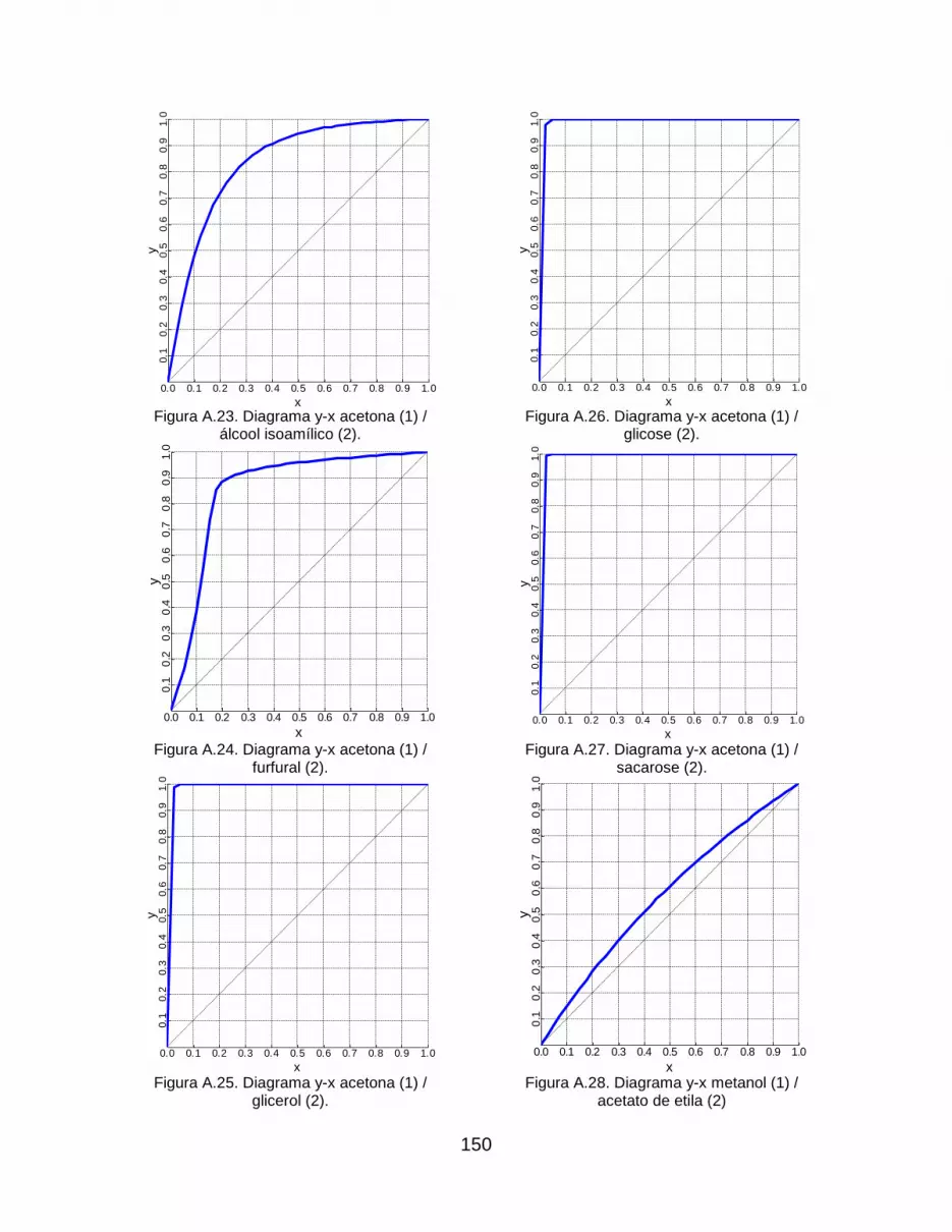
150


álcool isoamílico (2).


furfural (2).


glicerol (2).


glicose (2).


sacarose (2).

Figura A.28. Diagrama y-x metanol (1) /

acetato de etila (2)

x

y

0.0 0.1 0.2 0.3 0.4 0.5 0.6 0.7 0.8 0.9 1.0

0.1

0.2

0.3

0.4

0.5

0.6

0.7

0.8

0.9

1.0

x

y

0.0 0.1 0.2 0.3 0.4 0.5 0.6 0.7 0.8 0.9 1.0

0.1

0.2

0.3

0.4

0.5

0.6

0.7

0.8

0.9

1.0

x

y

0.0 0.1 0.2 0.3 0.4 0.5 0.6 0.7 0.8 0.9 1.0

0.1

0.2

0.3

0.4

0.5

0.6

0.7

0.8

0.9

1.0

x

y

0.0 0.1 0.2 0.3 0.4 0.5 0.6 0.7 0.8 0.9 1.0

0.1

0.2

0.3

0.4

0.5

0.6

0.7

0.8

0.9

1.0

x

y

0.0 0.1 0.2 0.3 0.4 0.5 0.6 0.7 0.8 0.9 1.0

0.1

0.2

0.3

0.4

0.5

0.6

0.7

0.8

0.9

1.0

x

y

0.0 0.1 0.2 0.3 0.4 0.5 0.6 0.7 0.8 0.9 1.0

0.1

0.2

0.3

0.4

0.5

0.6

0.7

0.8

0.9

1.0

151

. Figura A.29. Diagrama y-x metanol (1) /

etanol (2)

Figura A.30. Diagrama y-x metanol (1) / n-

propanol (2).


água (2).


isobutanol (2).

Figura A.33. Diagrama y-x metanol (1) / ácido

acético (2).


n-butanol (2).

x

y

0.0 0.1 0.2 0.3 0.4 0.5 0.6 0.7 0.8 0.9 1.0

0.1

0.2

0.3

0.4

0.5

0.6

0.7

0.8

0.9

1.0

x

y

0.0 0.1 0.2 0.3 0.4 0.5 0.6 0.7 0.8 0.9 1.0

0.1

0.2

0.3

0.4

0.5

0.6

0.7

0.8

0.9

1.0

x

y

0.0 0.1 0.2 0.3 0.4 0.5 0.6 0.7 0.8 0.9 1.0

0.1

0.2

0.3

0.4

0.5

0.6

0.7

0.8

0.9

1.0

x

y

0.0 0.1 0.2 0.3 0.4 0.5 0.6 0.7 0.8 0.9 1.0

0.1

0.2

0.3

0.4

0.5

0.6

0.7

0.8

0.9

1.0

x

y

0.0 0.1 0.2 0.3 0.4 0.5 0.6 0.7 0.8 0.9 1.0

0.1

0.2

0.3

0.4

0.5

0.6

0.7

0.8

0.9

1.0

x

y

0.0 0.1 0.2 0.3 0.4 0.5 0.6 0.7 0.8 0.9 1.0

0.1

0.2

0.3

0.4

0.5

0.6

0.7

0.8

0.9

1.0

152




furfural (2).


glicerol (2).


glicose (2).


sacarose (2).

Figura A.40. Diagrama y-x acetato de etila (1)

/ etanol (2).

x

y

0.0 0.1 0.2 0.3 0.4 0.5 0.6 0.7 0.8 0.9 1.0

0.1

0.2

0.3

0.4

0.5

0.6

0.7

0.8

0.9

1.0

x

y

0.0 0.1 0.2 0.3 0.4 0.5 0.6 0.7 0.8 0.9 1.0

0.1

0.2

0.3

0.4

0.5

0.6

0.7

0.8

0.9

1.0

x

y

0.0 0.1 0.2 0.3 0.4 0.5 0.6 0.7 0.8 0.9 1.0

0.1

0.2

0.3

0.4

0.5

0.6

0.7

0.8

0.9

1.0

x

y

0.0 0.1 0.2 0.3 0.4 0.5 0.6 0.7 0.8 0.9 1.0

0.1

0.2

0.3

0.4

0.5

0.6

0.7

0.8

0.9

1.0

x

y

0.0 0.1 0.2 0.3 0.4 0.5 0.6 0.7 0.8 0.9 1.0

0.1

0.2

0.3

0.4

0.5

0.6

0.7

0.8

0.9

1.0

x

y

0.0 0.1 0.2 0.3 0.4 0.5 0.6 0.7 0.8 0.9 1.0

0.1

0.2

0.3

0.4

0.5

0.6

0.7

0.8

0.9

1.0

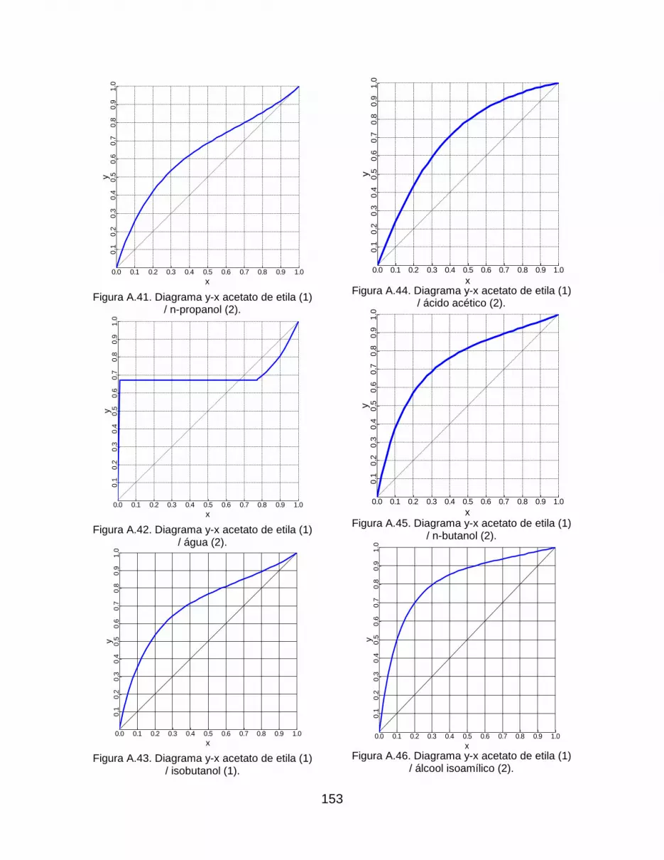
153


/ n-propanol (2).


/ água (2).


/ isobutanol (1).


/ ácido acético (2).


/ n-butanol (2).


/ álcool isoamílico (2).

x

y

0.0 0.1 0.2 0.3 0.4 0.5 0.6 0.7 0.8 0.9 1.0

0.1

0.2

0.3

0.4

0.5

0.6

0.7

0.8

0.9

1.0

x

y

0.0 0.1 0.2 0.3 0.4 0.5 0.6 0.7 0.8 0.9 1.0

0.1

0.2

0.3

0.4

0.5

0.6

0.7

0.8

0.9

1.0

x

y

0.0 0.1 0.2 0.3 0.4 0.5 0.6 0.7 0.8 0.9 1.0

0.1

0.2

0.3

0.4

0.5

0.6

0.7

0.8

0.9

1.0

x

y

0.0 0.1 0.2 0.3 0.4 0.5 0.6 0.7 0.8 0.9 1.0

0.1

0.2

0.3

0.4

0.5

0.6

0.7

0.8

0.9

1.0

x

y

0.0 0.1 0.2 0.3 0.4 0.5 0.6 0.7 0.8 0.9 1.0

0.1

0.2

0.3

0.4

0.5

0.6

0.7

0.8

0.9

1.0

x

y

0.0 0.1 0.2 0.3 0.4 0.5 0.6 0.7 0.8 0.9 1.0

0.1

0.2

0.3

0.4

0.5

0.6

0.7

0.8

0.9

1.0

154


/ furfural (2).


/ glicerol (2).

Figura A.49. Diagrama y-x com acetato de

etila (1) / glicose (2).


/ sacarose (2).

Figura A.51. Diagrama y-x etanol (1) /

n-propanol (2).


água (2).

x

y

0.0 0.1 0.2 0.3 0.4 0.5 0.6 0.7 0.8 0.9 1.0

0.1

0.2

0.3

0.4

0.5

0.6

0.7

0.8

0.9

1.0

x

y

0.0 0.1 0.2 0.3 0.4 0.5 0.6 0.7 0.8 0.9 1.0

0.1

0.2

0.3

0.4

0.5

0.6

0.7

0.8

0.9

1.0

x

y

0.0 0.1 0.2 0.3 0.4 0.5 0.6 0.7 0.8 0.9 1.0

0.1

0.2

0.3

0.4

0.5

0.6

0.7

0.8

0.9

1.0

x

y

0.0 0.1 0.2 0.3 0.4 0.5 0.6 0.7 0.8 0.9 1.0

0.1

0.2

0.3

0.4

0.5

0.6

0.7

0.8

0.9

1.0

x

y

0.0 0.1 0.2 0.3 0.4 0.5 0.6 0.7 0.8 0.9 1.0

0.1

0.2

0.3

0.4

0.5

0.6

0.7

0.8

0.9

1.0

x

y

0.0 0.1 0.2 0.3 0.4 0.5 0.6 0.7 0.8 0.9 1.0

0.1

0.2

0.3

0.4

0.5

0.6

0.7

0.8

0.9

1.0

155


isobutanol (2).

Figura A.54. Diagrama y-x etanol (1) / ácido

acético (2).

Figura A.55. Diagrama y-x etanol (1) / n-

butanol (2).

Figura A.56. Diagrama y-x etanol (1) / álcool

isoamílico (2).

. Figura A.57. Diagrama y-x etanol (1) /

furfural (2).


glicerol (2).

x

y

0.0 0.1 0.2 0.3 0.4 0.5 0.6 0.7 0.8 0.9 1.0

0.1

0.2

0.3

0.4

0.5

0.6

0.7

0.8

0.9

1.0

x

y

0.0 0.1 0.2 0.3 0.4 0.5 0.6 0.7 0.8 0.9 1.0

0.1

0.2

0.3

0.4

0.5

0.6

0.7

0.8

0.9

1.0

x

y

0.0 0.1 0.2 0.3 0.4 0.5 0.6 0.7 0.8 0.9 1.0

0.1

0.2

0.3

0.4

0.5

0.6

0.7

0.8

0.9

1.0

x

y

0.0 0.1 0.2 0.3 0.4 0.5 0.6 0.7 0.8 0.9 1.0

0.1

0.2

0.3

0.4

0.5

0.6

0.7

0.8

0.9

1.0

x

y

0.0 0.1 0.2 0.3 0.4 0.5 0.6 0.7 0.8 0.9 1.0

0.1

0.2

0.3

0.4

0.5

0.6

0.7

0.8

0.9

1.0

x

y

0.0 0.1 0.2 0.3 0.4 0.5 0.6 0.7 0.8 0.9 1.0

0.1

0.2

0.3

0.4

0.5

0.6

0.7

0.8

0.9

1.0

156


glicose (2).


sacarose (2).

Figura A.61. Diagrama y-x n-propanol (1) /

água (2).


isobutanol (2).




n-butanol (2).

x

y

0.0 0.1 0.2 0.3 0.4 0.5 0.6 0.7 0.8 0.9 1.0

0.1

0.2

0.3

0.4

0.5

0.6

0.7

0.8

0.9

1.0

x

y

0.0 0.1 0.2 0.3 0.4 0.5 0.6 0.7 0.8 0.9 1.0

0.1

0.2

0.3

0.4

0.5

0.6

0.7

0.8

0.9

1.0

x

y

0.0 0.1 0.2 0.3 0.4 0.5 0.6 0.7 0.8 0.9 1.0

0.1

0.2

0.3

0.4

0.5

0.6

0.7

0.8

0.9

1.0

x

y

0.0 0.1 0.2 0.3 0.4 0.5 0.6 0.7 0.8 0.9 1.0

0.1

0.2

0.3

0.4

0.5

0.6

0.7

0.8

0.9

1.0

x

y

0.0 0.2 0.4 0.6 0.8 1.0

0.1

0.2

0.3

0.4

0.5

0.6

0.7

0.8

0.9

1.0

x

y

0.0 0.1 0.2 0.3 0.4 0.5 0.6 0.7 0.8 0.9 1.0

0.1

0.2

0.3

0.4

0.5

0.6

0.7

0.8

0.9

1.0

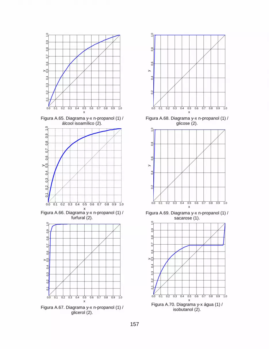
157




furfural (2).


glicerol (2).


glicose (2).


sacarose (1).

Figura A.70. Diagrama y-x água (1) /

isobutanol (2).

x

y

0.0 0.1 0.2 0.3 0.4 0.5 0.6 0.7 0.8 0.9 1.0

0.1

0.2

0.3

0.4

0.5

0.6

0.7

0.8

0.9

1.0

x

y

0.0 0.1 0.2 0.3 0.4 0.5 0.6 0.7 0.8 0.9 1.0

0.1

0.2

0.3

0.4

0.5

0.6

0.7

0.8

0.9

1.0

x

y

0.0 0.1 0.2 0.3 0.4 0.5 0.6 0.7 0.8 0.9 1.0

0.1

0.2

0.3

0.4

0.5

0.6

0.7

0.8

0.9

1.0

x

y

0.0 0.1 0.2 0.3 0.4 0.5 0.6 0.7 0.8 0.9 1.0

0.2

0.4

0.6

0.8

1.0

x

y

0.0 0.1 0.2 0.3 0.4 0.5 0.6 0.7 0.8 0.9 1.0

0.2

0.4

0.6

0.8

1.0

x

y

0.0 0.1 0.2 0.3 0.4 0.5 0.6 0.7 0.8 0.9 1.0

0.1

0.2

0.3

0.4

0.5

0.6

0.7

0.8

0.9

1.0

158

Figura A.71. Diagrama y-x água (1) / ácido

acético (2).


n-butanol (2).

Figura A.73. Diagrama y-x água (1) / álcool

isoamílico (2).

Figura A.74. Diagrama y-x água (1) / furfural

(2).


glicerol (2).


glicose (2).

x

y

0.0 0.1 0.2 0.3 0.4 0.5 0.6 0.7 0.8 0.9 1.0

0.1

0.2

0.3

0.4

0.5

0.6

0.7

0.8

0.9

1.0

x

y

0.0 0.1 0.2 0.3 0.4 0.5 0.6 0.7 0.8 0.9 1.0

0.1

0.2

0.3

0.4

0.5

0.6

0.7

0.8

0.9

1.0

x

y

0.0 0.1 0.2 0.3 0.4 0.5 0.6 0.7 0.8 0.9 1.0

0.1

0.2

0.3

0.4

0.5

0.6

0.7

0.8

0.9

1.0

x

y

0.0 0.1 0.2 0.3 0.4 0.5 0.6 0.7 0.8 0.9 1.0

0.1

0.2

0.3

0.4

0.5

0.6

0.7

0.8

0.9

1.0

x

y

0.0 0.1 0.2 0.3 0.4 0.5 0.6 0.7 0.8 0.9 1.0

0.1

0.2

0.3

0.4

0.5

0.6

0.7

0.8

0.9

1.0

x

y

0.0 0.1 0.2 0.3 0.4 0.5 0.6 0.7 0.8 0.9 1.0

0.1

0.2

0.3

0.4

0.5

0.6

0.7

0.8

0.9

1.0

159


sacarose (2).

Figura A.78. Diagrama y-x isobutanol (1) /



n-butanol (2).




furfural (2).


glicerol (2).

x

y

0.0 0.1 0.2 0.3 0.4 0.5 0.6 0.7 0.8 0.9 1.0

0.1

0.2

0.3

0.4

0.5

0.6

0.7

0.8

0.9

1.0

x

y

0.0 0.1 0.2 0.3 0.4 0.5 0.6 0.7 0.8 0.9 1.0

0.1

0.2

0.3

0.4

0.5

0.6

0.7

0.8

0.9

1.0

x

y

0.0 0.1 0.2 0.3 0.4 0.5 0.6 0.7 0.8 0.9 1.0

0.1

0.2

0.3

0.4

0.5

0.6

0.7

0.8

0.9

1.0

x

y

0.0 0.1 0.2 0.3 0.4 0.5 0.6 0.7 0.8 0.9 1.0

0.1

0.2

0.3

0.4

0.5

0.6

0.7

0.8

0.9

1.0

x

y

0.0 0.1 0.2 0.3 0.4 0.5 0.6 0.7 0.8 0.9 1.0

0.1

0.2

0.3

0.4

0.5

0.6

0.7

0.8

0.9

1.0

x

y

0.0 0.1 0.2 0.3 0.4 0.5 0.6 0.7 0.8 0.9 1.0

0.1

0.2

0.3

0.4

0.5

0.6

0.7

0.8

0.9

1.0

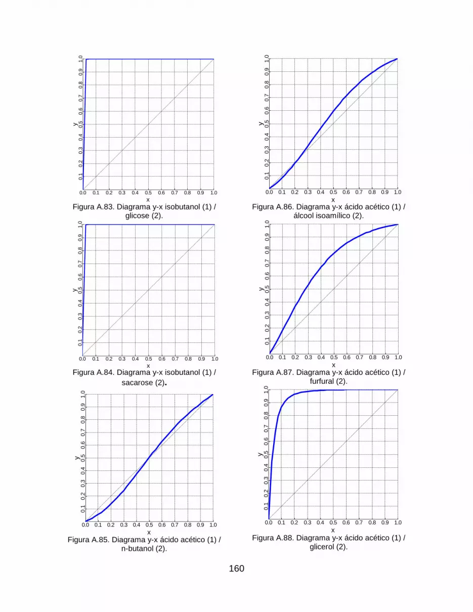
160


glicose (2).


sacarose (2).

Figura A.85. Diagrama y-x ácido acético (1) /

n-butanol (2).




furfural (2).


glicerol (2).

x

y

0.0 0.1 0.2 0.3 0.4 0.5 0.6 0.7 0.8 0.9 1.0

0.1

0.2

0.3

0.4

0.5

0.6

0.7

0.8

0.9

1.0

x

y

0.0 0.1 0.2 0.3 0.4 0.5 0.6 0.7 0.8 0.9 1.0

0.1

0.2

0.3

0.4

0.5

0.6

0.7

0.8

0.9

1.0

x

y

0.0 0.1 0.2 0.3 0.4 0.5 0.6 0.7 0.8 0.9 1.0

0.1

0.2

0.3

0.4

0.5

0.6

0.7

0.8

0.9

1.0

x

y

0.0 0.1 0.2 0.3 0.4 0.5 0.6 0.7 0.8 0.9 1.0

0.1

0.2

0.3

0.4

0.5

0.6

0.7

0.8

0.9

1.0

x

y

0.0 0.1 0.2 0.3 0.4 0.5 0.6 0.7 0.8 0.9 1.0

0.1

0.2

0.3

0.4

0.5

0.6

0.7

0.8

0.9

1.0

x

y

0.0 0.1 0.2 0.3 0.4 0.5 0.6 0.7 0.8 0.9 1.0

0.1

0.2

0.3

0.4

0.5

0.6

0.7

0.8

0.9

1.0

161


glicose (2).


sacarose (2).

Figura A.91. Diagrama y-x n-butanol (1) /



furfural (2).


glicerol (2).


glicose (2).

x

y

0.0 0.1 0.2 0.3 0.4 0.5 0.6 0.7 0.8 0.9 1.0

0.1

0.2

0.3

0.4

0.5

0.6

0.7

0.8

0.9

1.0

x

y

0.0 0.1 0.2 0.3 0.4 0.5 0.6 0.7 0.8 0.9 1.0

0.1

0.2

0.3

0.4

0.5

0.6

0.7

0.8

0.9

1.0

x

y

0.0 0.1 0.2 0.3 0.4 0.5 0.6 0.7 0.8 0.9 1.0

0.1

0.2

0.3

0.4

0.5

0.6

0.7

0.8

0.9

1.0

x

y

0.0 0.1 0.2 0.3 0.4 0.5 0.6 0.7 0.8 0.9 1.0

0.1

0.2

0.3

0.4

0.5

0.6

0.7

0.8

0.9

1.0

x

y

0.0 0.1 0.2 0.3 0.4 0.5 0.6 0.7 0.8 0.9 1.0

0.1

0.2

0.3

0.4

0.5

0.6

0.7

0.8

0.9

1.0

x

y

0.0 0.1 0.2 0.3 0.4 0.5 0.6 0.7 0.8 0.9 1.0

0.1

0.2

0.3

0.4

0.5

0.6

0.7

0.8

0.9

1.0

162


sacarose (2).

Figura A.96. Diagrama y-x álcool isoamílico

(1) / furfural (2).


(1) / glicerol (2).


(1) / glicose (2).


(1) / sacarose (2).

Figura A.100. Diagrama y-x furfural (1) /

glicerol (2).

x

y

0.0 0.1 0.2 0.3 0.4 0.5 0.6 0.7 0.8 0.9 1.0

0.1

0.2

0.3

0.4

0.5

0.6

0.7

0.8

0.9

1.0

x

y

0.0 0.1 0.2 0.3 0.4 0.5 0.6 0.7 0.8 0.9 1.0

0.1

0.2

0.3

0.4

0.5

0.6

0.7

0.8

0.9

1.0

x

y

0.0 0.1 0.2 0.3 0.4 0.5 0.6 0.7 0.8 0.9 1.0

0.1

0.2

0.3

0.4

0.5

0.6

0.7

0.8

0.9

1.0

x

y

0.0 0.1 0.2 0.3 0.4 0.5 0.6 0.7 0.8 0.9 1.0

0.1

0.2

0.3

0.4

0.5

0.6

0.7

0.8

0.9

1.0

x

y

0.0 0.1 0.2 0.3 0.4 0.5 0.6 0.7 0.8 0.9 1.0

0.1

0.2

0.3

0.4

0.5

0.6

0.7

0.8

0.9

1.0

x

y

0.0 0.1 0.2 0.3 0.4 0.5 0.6 0.7 0.8 0.9 1.0

0.1

0.2

0.3

0.4

0.5

0.6

0.7

0.8

0.9

1.0

163


glicose (2).


sacarose (2).

Figura A.103. Diagrama y-x glicerol (1) /

glicose (2).

Figura A.104. Diagrama y-x glicerol (1) /

sacarose (2).

Figura A.105. Diagrama y-x glicose (1) /

sacarose (2).


cicloexano (2).

x

y

0.0 0.1 0.2 0.3 0.4 0.5 0.6 0.7 0.8 0.9 1.0

0.1

0.2

0.3

0.4

0.5

0.6

0.7

0.8

0.9

1.0

x

y

0.0 0.1 0.2 0.3 0.4 0.5 0.6 0.7 0.8 0.9 1.0

0.1

0.2

0.3

0.4

0.5

0.6

0.7

0.8

0.9

1.0

x

y

0.0 0.1 0.2 0.3 0.4 0.5 0.6 0.7 0.8 0.9 1.0

0.1

0.2

0.3

0.4

0.5

0.6

0.7

0.8

0.9

1.0

x

y

0.0 0.1 0.2 0.3 0.4 0.5 0.6 0.7 0.8 0.9 1.0

0.1

0.2

0.3

0.4

0.5

0.6

0.7

0.8

0.9

1.0

x

y

0.0 0.1 0.2 0.3 0.4 0.5 0.6 0.7 0.8 0.9 1.0

0.1

0.2

0.3

0.4

0.5

0.6

0.7

0.8

0.9

1.0

x

y

0.0 0.1 0.2 0.3 0.4 0.5 0.6 0.7 0.8 0.9 1.0

0.1

0.2

0.3

0.4

0.5

0.6

0.7

0.8

0.9

1.0

164

Figura A.107. Diagrama y-x cicloexano (1) /

água (2).


etilenoglicol (2).

Figura A.109. Diagrama y-x água (1) / etilenoglicol (2).

Os diagramas binários foram analisados de forma a observar as não

idealidades presentes no sistema. Os binários foram classificados de acordo com

a não idealidade através da Tabela A.1.

x

y

0.0 0.1 0.2 0.3 0.4 0.5 0.6 0.7 0.8 0.9 1.0

0.1

0.2

0.3

0.4

0.5

0.6

0.7

0.8

0.9

1.0

x

y

0.0 0.1 0.2 0.3 0.4 0.5 0.6 0.7 0.8 0.9 1.0

0.1

0.2

0.3

0.4

0.5

0.6

0.7

0.8

0.9

1.0

x

y

0.0 0.1 0.2 0.3 0.4 0.5 0.6 0.7 0.8 0.9 1.0

0.1

0.2

0.3

0.4

0.5

0.6

0.7

0.8

0.9

1.0

165

Tabela A.1. Não idealidades observadas no sistema.

Não idealidade Binário

Azeotropia

Acetona/Metanol Acetato de etila/Etanol Acetato de etila/Água Etanol/Água n-Propanol/Água Água/Isobutanol Água/Furfural Água/n-Butanol

Água/Álcool isoamílico Isobutanol/Ácido acético Ácido acético/n-Butanol Ácido acético/Álcool isoamílico Álcool isoamílico/Glicerol Etanol/Cicloexano Cicloexano/Água

Formação de Duas Fases Líquidas

Acetato de etila/Água n-Propanol/Água Água/Isobutanol Água/Furfural

Água/n-Butanol Água/Álcool isoamílico Álcool isoamílico/Glicerol Cicloexano/Água

Baixa Volatilidade Relativa

Acetona/Metanol Acetona/Acetato de etila Acetona/Etanol Metanol/Acetato de etila Metanol/Etanol Acetato de etila/Etanol Etanol/n-Propanol n-Propanol/Isobutanol

n-Propanol/Ácido acético n-Propanol/n-Butanol Água/Ácido acético Isobutanol/Ácido acético Isobutanol/n-Butanol Ácido acético/n-Butanol Ácido acético/Álcool isoamílico n-Butanol/Álcool Isoamílico

Alta Volatilidade Relativa

Acetaldeído/Água Acetaldeído/Glicerol Acetaldeído/Glicose Acetaldeído/Sacarose Acetona/Glicerol Acetona/Glicose Acetona/Sacarose Metanol/Glicerol Metanol/Glicose Metanol/Sacarose Acetato de etila/Glicerol Acetato de etila /Glicose Acetato de etila /Sacarose Etanol/Glicerol Etanol/Glicose Etanol/Sacarose n-Propanol /Glicerol

n-Propanol /Glicose n-Propanol /Sacarose Água/Glicerol Água /Glicose Água /Sacarose Isobutanol/Glicerol Isobutanol/Glicose Isobutanol/Sacarose Ácido acético/Glicose Ácido acético/Sacarose n-Butanol/Glicose n-Butanol/Sacarose Álcool isoamílico/Glicose Álcool isoamílico/Sacarose Furfural/Glicose Furfural/Sacarose

Documents

Simulação de colunas de destilação convencional, extrativa e azeotropica no processo de produção de bioetanol atraves da modelagem de não equilibrio e da modelagem de estagios