Embed Size (px)
Citation preview
Computer Networks 44 (2004) 631–641
www.elsevier.com/locate/comnet
Simulation analysis of RED with short lived TCP connections
Eitan Altman a,*, Tania Jim�enez b
a INRIA, BP93, 2004 Route des Lucioles, 06902 Sophia Antipolis Cedex, Franceb CESIMO, Facultad de Ingeniera, Univ. de Los Andes, 5101 M�erida, Venezuela
Received 5 October 2003; received in revised form 6 October 2003; accepted 8 October 2003
Responsible Editor: S. Low
Abstract
Several objectives have been identified in developing the random early drop (RED): decreasing queueing delay,
increasing throughput, and increasing fairness between short and long lived connections. It has been believed that
indeed the drop probability of a packet in RED does not depend on the size of the file to which it belongs. In this paper
we study the fairness properties of RED where fairness is taken with respect to the size of the transferred file. We focus
on short lived TCP sessions. Our findings are that (i) in terms of loss probabilities, RED is unfair: it favors short
sessions, (ii) RED is fairer in terms of the average throughput of a session (as a function of its size) than in terms of loss
probabilities. We study various loading regimes, with various versions of RED.
� 2003 Elsevier B.V. All rights reserved.
Keywords: RED; TCP; Buffer management; Simulations; Fairness
1. Introduction
One of the objectives of random early drop
(RED) has been to get rid of the bias of drop-tail
buffers against bursty traffic [3]. It has been con-
firmed in [4, Section IX] that indeed RED gets rid
of this bias and is fair in terms of fraction of lost
packets. This has been demonstrated in a frame-work where both bursty as well as ‘‘smooth’’ traffic
were taken as permanent FTP connections. The
higher burstiness was obtained by using smaller
windows and longer round-trip times. In a recent
paper [7], the authors show that conclusions drawn
* Corresponding author. Tel.: +33-4-92-38-77-86.
E-mail address: [email protected] (E. Altman).
1389-1286/$ - see front matter � 2003 Elsevier B.V. All rights reserv
doi:10.1016/j.comnet.2003.08.003
from simulating permanent TCP connections can
be qualitatively quite different than those obtained
from simulations of transfers that have large time
scale variability. The latter is obtained by replac-
ing the infinite source model by ones in which
transfered files have heavy-tailed distributions.
This motivated us to question the qualitative
conclusions drawn in [4] and restudy the fairnessissue using Pareto distributed file sizes. We are
interested in the following questions: (i) how does
the drop probability of a packet depend on the file
size? (ii) how does the average throughput expe-
rienced by a file depend on its size?
If we identify arrival of packets from a file as a
‘‘batch’’ (which is justified by our simulations),
then the fairness in terms of the file size also answerthe question of fairness in terms of batch sizes.
ed.
632 E. Altman, T. Jim�enez / Computer Networks 44 (2004) 631–641
Our main findings are that in terms of loss
probabilities, RED is biased against long files.
Furthermore, we show that this bias increases as the
workload decreases. We study this phenomenon
and provide an explanation for it. We further show
that RED is fairer in terms of throughput than it isin terms of loss probabilities. When comparing to
drop-tail buffers, we see that for all loads, RED has
smaller loss probabilities for almost all transfer si-
zes; the drop-tail buffer is more fair in terms of drop
probabilities (as a function of the transfer size) since
it has many more drops for short file transfers. In
terms of throughput, RED is slightly fairer than the
drop-tail buffer. Our conclusions similar for fourdifferent variants of RED that we tested.
We briefly mention some related work. Fair
RED (FRED) is proposed in [10] which needs
however to keep some per-active-flow states. 1 Its
performance is analyzed by simulating permanent
TCP connections. In [14], stabilized RED (SRED)
is proposed, requiring per-flow state information
too. Unlike RED, the drop probabilities dependonly on the instantaneous buffer occupation and on
the estimated number of active flows. Fairness
according to the transfer size is not considered
there. [2] analyzes biasness with respect to bursty
traffic. Both smooth as well as bursty traffic are
modeled as Poisson processes, but in the smooth
case each arrival corresponds to a single packet,
where as in the bursty traffic case each arrivalbrings a batch of B packets. The conclusions of the
paper are that indeed RED decreases the bias
against bursty traffic. The traffic models used are
not closed loop (they do not adapt to congestion),
and as we learn from [1] and [7, Section 4], quali-
tative behavior of closed loop traffic can be quite
different from open loop. Although there are also
some TCP simulations of RED in [2], these usepermanent connections. Other papers studied RED
using long lived TCP connections [6,9,11–13,15–
17] as well as short lived connections [8,17]. But the
fairness issue is not examined in these references.
1 It is argued in [10] that dropping ‘‘fairly’’ packets does not
guarantee fair bandwidth sharing. Interestingly, our simula-
tions show that bandwidth sharing is fairer in RED than could
be expected because RED is unfair in dropping packets.
We study the standard as well as the adaptive
RED version, both with and without the gentle
option of RED. 2 We introduce the model and
simulation setup in Section 2, present some pre-
liminary simulation results in Section 3, then
present the fairness results in terms of the lossprobabilities in Section 4 and in terms of the
throughput in Section 5. The analysis of these re-
sults and explanation of the causes for the ob-
served behavior are given in Section 6, and we end
with a concluding section.
2. Model and simulation setup
2.1. Traffic model and topology
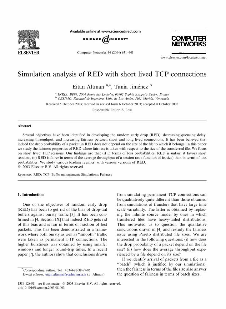
There are X source nodes (X is determined be-
low) connected to a bottleneck link N through
which the packets are forwarded to a common
destination D. We consider transfer of files from
each source node whose distribution is Pareto withan average size of 30 kbytes and with shape
parameter of 1.1. 3 From each node, the time be-
tween beginning of transmissions of files has an
exponential distribution with average of 0.9 s.
Thus a source can be sending simultaneously
packets belonging to more than one connection.
The bottleneck link N � D has a delay of 1 ms and
a queue of size 50 packets. The rate of the link is1.8 Mbps (it will later be increased up to 2.5 Mbps
in order to study the dependence of the perfor-
mance in the load of the system). The other links,
i.e. between the sources and N , have all 100 Mbps
bandwidth and a delay of 1 ms. The network is
depicted in Fig. 1. The average input rate of data
information into the bottleneck link from each
node is 30 · 103 · 8/0.9 s¼ 266.67 kbps. We tookpacket sizes of 500 bytes, so with an additional
overhead of 40 bytes, their size is 540 bytes. Tak-
ing this into account, the total transmission rate of
bits (without counting the retransmissions) from
each source is 288 kbps. Thus the system can
2 http://www.icir.org/floyd/red/gentle.html.3 Recall that for Pareto distribution, Prðsize > sÞ ¼ ðk=sÞb
and E½size� ¼ bk=ðb � 1Þ where b is the shape parameter; thus
the parameter k equals to 2727.27.
1500
2000
2500
Size of connections
SourceNode
SourceNode
SourceNode
SourceNode
SourceNode
N
100Mbps
100Mbps
100Mbps
1 msec
1 msec
1 msec 1 msec
1.8-2.5Mbps NodeDestination
D
Fig. 1. Network topology.
E. Altman, T. Jim�enez / Computer Networks 44 (2004) 631–641 633
support at most X ¼ 6 input nodes in order that
the number of sessions does not grow to infinity.The total arrival rate of bits (without retransmis-
sions) is then 1.728 Mbps, so we work in a heavy
load regime close to 1, i.e. q ¼ 1:728=1:8 ¼ 0:96.Increasing the bottleneck capacity to 2.5 Mbps will
allow us to check the light load regime where
q ¼ 1:728=2:5 ¼ 0:6912. Our simulations lasted
2500 s each so as to gather sufficient information
on sessions of different sizes.
2.2. RED configuration and parameters
We shall consider four variants of RED and
compare them to a drop-tail buffer: the standard
RED [4], the adaptive RED [5], and each of these
with and without the ‘‘gentle’’ option of RED. The
configurations are as follows:
(i) Standard RED: We have used the automatic
configuration option of ns (that is set by de-
fault). This gave the following values:
maxth ¼ 15, minth ¼ 5, wq ¼ 0:0004 and
maxp ¼ 0:1. 4
4 Recall that with standard RED, packets start to get
rejected when the averaged queue size avg exceeds minth, and
the loss probability increases linearly from 0 to maxp as the
average queue size increases between minth and maxth. When it
exceeds maxth the dropping probability is one. The avg
parameter is initially set to zero. Then with each arriving
packet, avg is updated to the value ð1� wqÞavgþ wqq where q isthe actual queue size and wq is some small constant.
(ii) Adaptive RED: [5] The value of the parameter
maxp is adapted so as to keep the average
queue size within a target range of half way be-
tween minth and maxth, and it is constrained to
the range of ½0:01; 0:5�. The adaptation is doneusing an additive increase multiplicative de-
crease policy with parameters a and b, respec-tively. We use the default ns parameters of
adaptive RED (in particular, we have
a ¼ 0:01 and b ¼ 0:9).(iii) Gentle RED: In the gentle RED option, once
the averaged queue size exceeds maxth, the
drop probability does not jump to 1, but in-creases linearly (‘‘gently’’) to 1 as the average
queue size increases to twice maxth.
All our simulations use the same common ar-
rival process of sessions as well as the same size of
files (same seeds and generators) so that we can
compare easier the effects of the RED version and
bandwidth.
2.3. On the reliability of the simulations
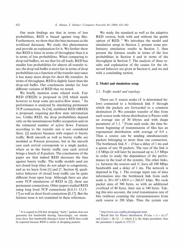
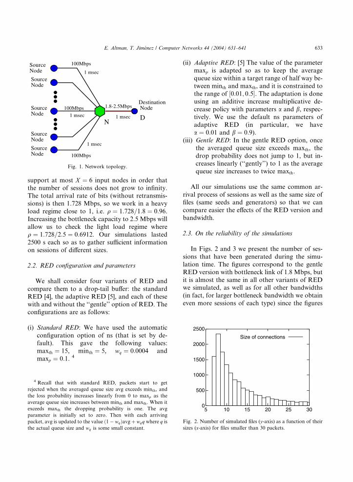
In Figs. 2 and 3 we present the number of ses-
sions that have been generated during the simu-
lation time. The figures correspond to the gentle
RED version with bottleneck link of 1.8 Mbps, but
it is almost the same in all other variants of REDwe simulated, as well as for all other bandwidths
(in fact, for larger bottleneck bandwidth we obtain
even more sessions of each type) since the figures
0
500
1000
5 10 15 20 25 30
Fig. 2. Number of simulated files (y-axis) as a function of their
sizes (x-axis) for files smaller than 30 packets.
0
1
2
3
4
5
6
735 740 745 750 755
heavy loadlight load
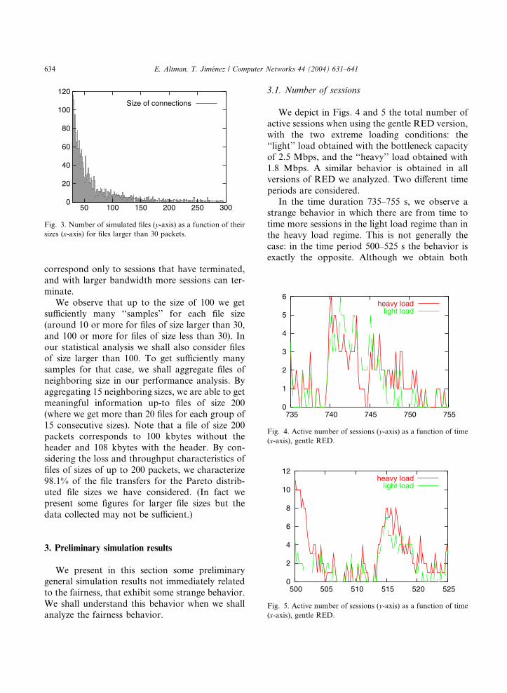
Fig. 4. Active number of sessions (y-axis) as a function of time
(x-axis), gentle RED.
8
10
12heavy load
light load
0
20
40
60
80
100
120
50 100 150 200 250 300
Size of connections
Fig. 3. Number of simulated files (y-axis) as a function of their
sizes (x-axis) for files larger than 30 packets.
634 E. Altman, T. Jim�enez / Computer Networks 44 (2004) 631–641
correspond only to sessions that have terminated,
and with larger bandwidth more sessions can ter-
minate.
We observe that up to the size of 100 we get
sufficiently many ‘‘samples’’ for each file size
(around 10 or more for files of size larger than 30,
and 100 or more for files of size less than 30). Inour statistical analysis we shall also consider files
of size larger than 100. To get sufficiently many
samples for that case, we shall aggregate files of
neighboring size in our performance analysis. By
aggregating 15 neighboring sizes, we are able to get
meaningful information up-to files of size 200
(where we get more than 20 files for each group of
15 consecutive sizes). Note that a file of size 200packets corresponds to 100 kbytes without the
header and 108 kbytes with the header. By con-
sidering the loss and throughput characteristics of
files of sizes of up to 200 packets, we characterize
98.1% of the file transfers for the Pareto distrib-
uted file sizes we have considered. (In fact we
present some figures for larger file sizes but the
data collected may not be sufficient.)
0
2
4
6
500 505 510 515 520 525
Fig. 5. Active number of sessions (y-axis) as a function of time
(x-axis), gentle RED.
3. Preliminary simulation results
We present in this section some preliminary
general simulation results not immediately related
to the fairness, that exhibit some strange behavior.
We shall understand this behavior when we shallanalyze the fairness behavior.
3.1. Number of sessions
We depict in Figs. 4 and 5 the total number of
active sessions when using the gentle RED version,
with the two extreme loading conditions: the‘‘light’’ load obtained with the bottleneck capacity
of 2.5 Mbps, and the ‘‘heavy’’ load obtained with
1.8 Mbps. A similar behavior is obtained in all
versions of RED we analyzed. Two different time
periods are considered.
In the time duration 735–755 s, we observe a
strange behavior in which there are from time to
time more sessions in the light load regime than inthe heavy load regime. This is not generally the
case: in the time period 500–525 s the behavior is
exactly the opposite. Although we obtain both
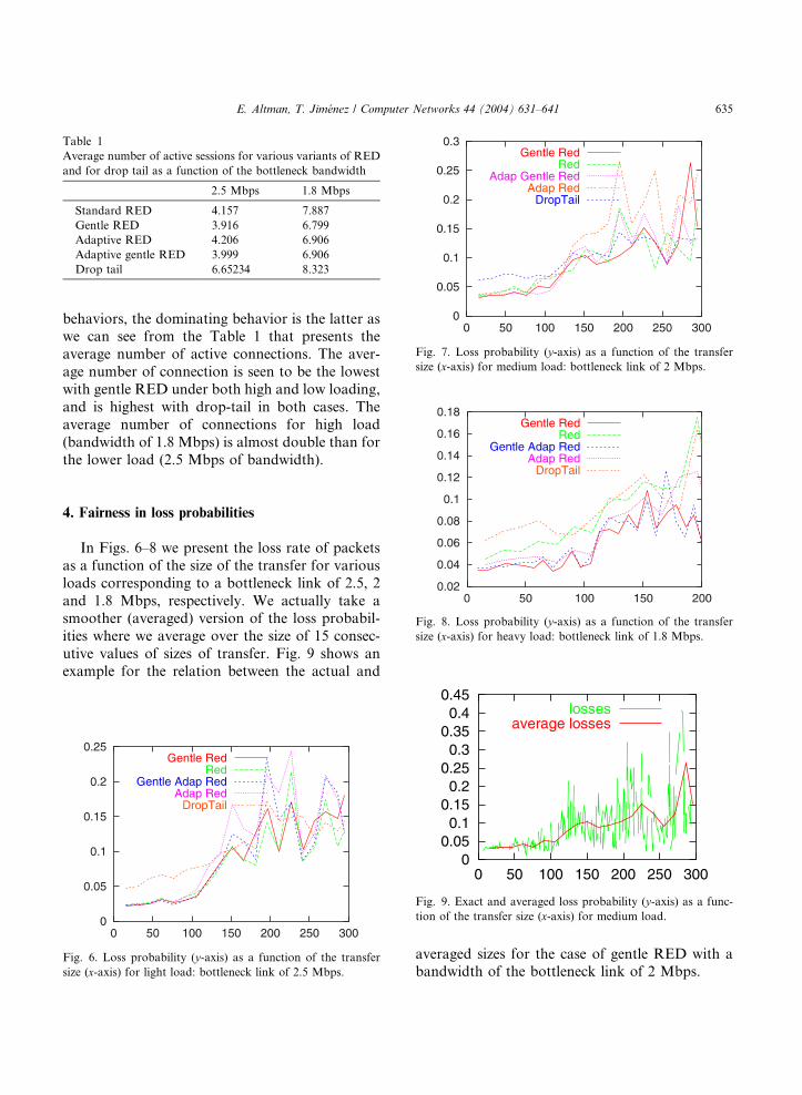
Table 1
Average number of active sessions for various variants of RED
and for drop tail as a function of the bottleneck bandwidth
2.5 Mbps 1.8 Mbps
Standard RED 4.157 7.887
Gentle RED 3.916 6.799
Adaptive RED 4.206 6.906
Adaptive gentle RED 3.999 6.906
Drop tail 6.65234 8.323
Fig. 7. Loss probability (y-axis) as a function of the transfer
size (x-axis) for medium load: bottleneck link of 2 Mbps.
E. Altman, T. Jim�enez / Computer Networks 44 (2004) 631–641 635
behaviors, the dominating behavior is the latter aswe can see from the Table 1 that presents the
average number of active connections. The aver-
age number of connection is seen to be the lowest
with gentle RED under both high and low loading,
and is highest with drop-tail in both cases. The
average number of connections for high load
(bandwidth of 1.8 Mbps) is almost double than for
the lower load (2.5 Mbps of bandwidth).
Fig. 8. Loss probability (y-axis) as a function of the transfer
size (x-axis) for heavy load: bottleneck link of 1.8 Mbps.
4. Fairness in loss probabilities
In Figs. 6–8 we present the loss rate of packets
as a function of the size of the transfer for various
loads corresponding to a bottleneck link of 2.5, 2
and 1.8 Mbps, respectively. We actually take asmoother (averaged) version of the loss probabil-
ities where we average over the size of 15 consec-
utive values of sizes of transfer. Fig. 9 shows an
example for the relation between the actual and
Fig. 6. Loss probability (y-axis) as a function of the transfer
size (x-axis) for light load: bottleneck link of 2.5 Mbps.
00.050.1
0.150.2
0.250.3
0.350.4
0.45
0 50 100 150 200 250 300
lossesaverage losses
Fig. 9. Exact and averaged loss probability (y-axis) as a func-
tion of the transfer size (x-axis) for medium load.
averaged sizes for the case of gentle RED with abandwidth of the bottleneck link of 2 Mbps.
0
0.02
0.04
0.06
0.08
0.1
0.12
0.14
0.16
0.18
0 50 100 150 200
4ms8ms
20ms40ms80ms
120ms
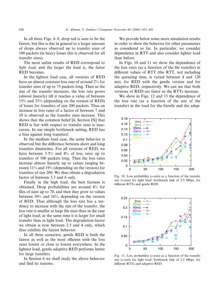
Fig. 10. Loss probability (y-axis) as a function of the transfer
size (x-axis) for light load: bottleneck link of 2.5 Mbps, for
different RTTs and gentle RED.
0
0.05
0.1
0.15
0.2
0.25
0 50 100 150 200
8ms20ms40ms80ms
120ms
Fig. 11. Loss probability (y-axis) as a function of the transfer
size (x-axis) for light load: bottleneck link of 2.5 Mbps, for
different RTTs and adaptive RED.
636 E. Altman, T. Jim�enez / Computer Networks 44 (2004) 631–641
In all three Figs. 6–8, drop tail is seen to be the
fairest, but this is due in general to a larger amount
of drops always observed up to transfer sizes of
100 packets (in heavy losses this is observed for all
transfer sizes).
The most unfair results of RED correspond tolight load, and the larger the load is, the fairer
RED becomes.
In the lightest load case, all versions of RED
have an almost constant loss rate of around 2% for
transfer sizes of up to 75 packets long. Then as the
size of the transfer increases, the loss rate grows
(almost linearly) till it reaches a value of between
15% and 21% (depending on the version of RED)of losses for transfers of size 200 packets. Thus an
increase in loss rates of a factor of between 7 and
10 is observed as the transfer sizes increase. This
shows that the common belief [4, Section IX] that
RED is fair with respect to transfer sizes is inac-
curate. In our simple bottleneck setting, RED has
a bias against long transfers!
In the medium load case, the same behavior isobserved but the difference between short and long
transfers diminishes. For all versions of RED, we
have between 3.3% and 4% of loss rates up to
transfers of 100 packets long. Then the loss rates
increase almost linearly up to values ranging be-
tween 11% and 19% (depending on the version) for
transfers of size 200. We thus obtain a degradation
factor of between 3.3 and 6 only.Finally in the high load, the best fairness is
obtained. Drop probabilities are around 4% for
files of sizes up to 70, and then they grow to values
between 10% and 16%, depending on the version
of RED. Thus although the loss rate has a ten-
dency to increase with the size of the transfer, the
loss rate is smaller at large file sizes than in the case
of light load; at the same time it is larger for smalltransfer than in light load. The degradation factor
we obtain is now between 2.5 and 4 only, which
thus exhibits the fairest behavior.
In all three scenarios, gentle RED is both the
fairest as well as the most efficient with the loss
rates lowest or close to lowest everywhere. In the
lightest load, gentle adaptive RED performs better
for large transfers.In Section 6 we shall study the above behavior
and find its reasons.
We provide below some more simulation results
in order to show the behavior for other parameters
as considered so far. In particular, we consider
dependence in RTT and also consider lighter load
than before.
In Figs. 10 and 11 we show the dependence ofthe loss rates (as a function of the file transfer) in
different values of RTT (the RTT, not including
the queueing time, is varied between 4 and 120
ms), for RED with the gentle version and for
adaptive RED, respectively. We can see that both
versions of RED are fairer as the RTTs increase.
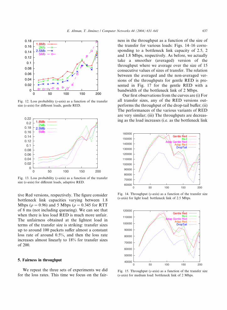
We show in Figs. 12 and 13 the dependence of
the loss rate (as a function of the size of thetransfer) in the load for the Gentle and the adap-
0
0.02
0.04
0.06
0.08
0.1
0.12
0.14
0.16
0.18
0 50 100 150 200
1.8Mb2Mb
2.5Mb5Mb
Fig. 12. Loss probability (y-axis) as a function of the transfer
size (x-axis) for different loads, gentle RED.
Fig. 13. Loss probability (y-axis) as a function of the transfer
size (x-axis) for different loads, adaptive RED.
Fig. 14. Throughput (y-axis) as a function of the transfer size
(x-axis) for light load: bottleneck link of 2.5 Mbps.
E. Altman, T. Jim�enez / Computer Networks 44 (2004) 631–641 637
tive Red versions, respectively. The figure consider
bottleneck link capacities varying between 1.8
Mbps (q ¼ 0:96) and 5 Mbps (q ¼ 0:345 for RTT
of 8 ms (not including queueing). We can see that
when there is less load RED is much more unfair.
The unfairness obtained at the lightest load interms of the transfer size is striking: transfer sizes
up to around 100 packets suffer almost a constant
loss rate of around 0.5%, and then the loss rate
increases almost linearly to 18% for transfer sizes
of 200.
Fig. 15. Throughput (y-axis) as a function of the transfer size
(x-axis) for medium load: bottleneck link of 2 Mbps.
5. Fairness in throughput
We repeat the three sets of experiments we did
for the loss rates. This time we focus on the fair-
ness in the throughput as a function of the size of
the transfer for various loads: Figs. 14–16 corre-
sponding to a bottleneck link capacity of 2.5, 2
and 1.8 Mbps, respectively. As before, we actually
take a smoother (averaged) version of the
throughput where we average over the size of 15consecutive values of sizes of transfer. The relation
between the averaged and the non-averaged ver-
sions of the throughputs for gentle RED is pre-
sented in Fig. 17 for the gentle RED with a
bandwidth of the bottleneck link of 2 Mbps.
Our first observations from the curves are (i) For
all transfer sizes, any of the RED versions out-
performs the throughput of the drop-tail buffer; (ii)The performances of the various variants of RED
are very similar; (iii) The throughputs are decreas-
ing as the load increases (i.e. as the bottleneck link
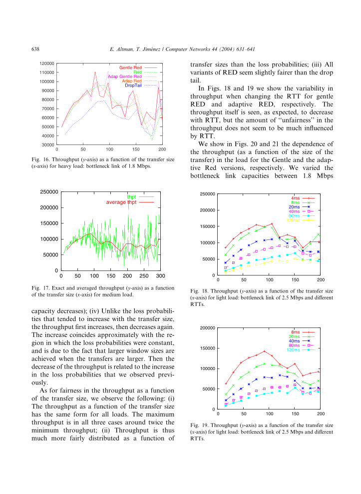
Fig. 16. Throughput (y-axis) as a function of the transfer size
(x-axis) for heavy load: bottleneck link of 1.8 Mbps.
0
50000
100000
150000
200000
250000
0 50 100 150 200 250 300
thptaverage thpt
Fig. 17. Exact and averaged throughput (y-axis) as a function
of the transfer size (x-axis) for medium load.
0
50000
100000
150000
200000
250000
0 50 100 150 200
4ms8ms
20ms40ms80ms
120ms
Fig. 18. Throughput (y-axis) as a function of the transfer size
(x-axis) for light load: bottleneck link of 2.5 Mbps and different
RTTs.
0
50000
100000
150000
200000
0 50 100 150 200
8ms20ms40ms80ms
120ms
Fig. 19. Throughput (y-axis) as a function of the transfer size
(x-axis) for light load: bottleneck link of 2.5 Mbps and different
RTTs.
638 E. Altman, T. Jim�enez / Computer Networks 44 (2004) 631–641
capacity decreases); (iv) Unlike the loss probabili-ties that tended to increase with the transfer size,
the throughput first increases, then decreases again.
The increase coincides approximately with the re-
gion in which the loss probabilities were constant,
and is due to the fact that larger window sizes are
achieved when the transfers are larger. Then the
decrease of the throughput is related to the increase
in the loss probabilities that we observed previ-ously.
As for fairness in the throughput as a function
of the transfer size, we observe the following: (i)
The throughput as a function of the transfer size
has the same form for all loads. The maximum
throughput is in all three cases around twice the
minimum throughput; (ii) Throughput is thus
much more fairly distributed as a function of
transfer sizes than the loss probabilities; (iii) All
variants of RED seem slightly fairer than the drop
tail.
In Figs. 18 and 19 we show the variability in
throughput when changing the RTT for gentle
RED and adaptive RED, respectively. Thethroughput itself is seen, as expected, to decrease
with RTT, but the amount of ‘‘unfairness’’ in the
throughput does not seem to be much influenced
by RTT.
We show in Figs. 20 and 21 the dependence of
the throughput (as a function of the size of the
transfer) in the load for the Gentle and the adap-
tive Red versions, respectively. We varied thebottleneck link capacities between 1.8 Mbps
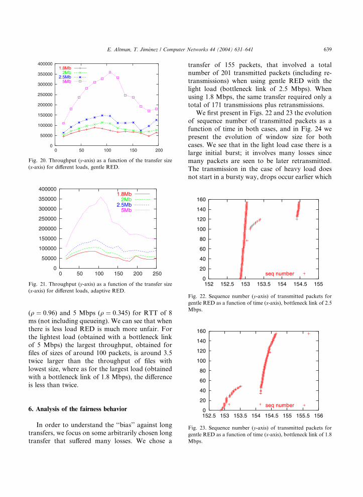
Fig. 20. Throughput (y-axis) as a function of the transfer size
(x-axis) for different loads, gentle RED.
Fig. 21. Throughput (y-axis) as a function of the transfer size
(x-axis) for different loads, adaptive RED.
0
20
40
60
80
100
120
140
160
152 152.5 153 153.5 154 154.5 155
seq number
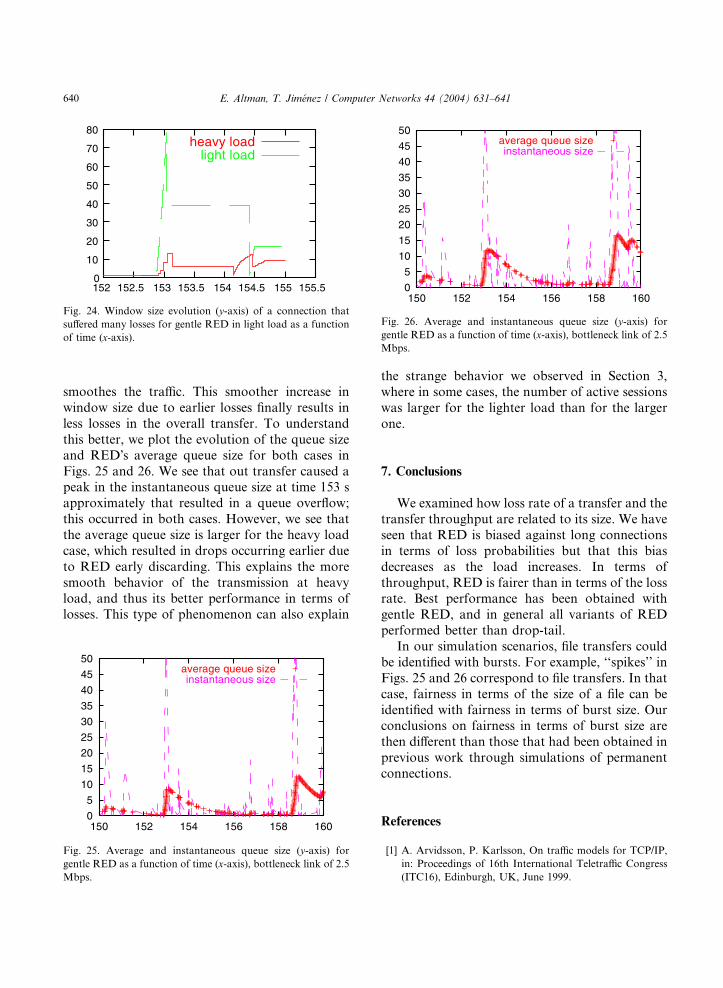
Fig. 22. Sequence number (y-axis) of transmitted packets for
gentle RED as a function of time (x-axis), bottleneck link of 2.5
Mbps.
60
80
100
120
140
160
E. Altman, T. Jim�enez / Computer Networks 44 (2004) 631–641 639
(q ¼ 0:96) and 5 Mbps (q ¼ 0:345) for RTT of 8
ms (not including queueing). We can see that when
there is less load RED is much more unfair. For
the lightest load (obtained with a bottleneck link
of 5 Mbps) the largest throughput, obtained for
files of sizes of around 100 packets, is around 3.5twice larger than the throughput of files with
lowest size, where as for the largest load (obtained
with a bottleneck link of 1.8 Mbps), the difference
is less than twice.
0
20
40
152.5 153 153.5 154 154.5 155 155.5 156
seq number
Fig. 23. Sequence number (y-axis) of transmitted packets for
gentle RED as a function of time (x-axis), bottleneck link of 1.8
Mbps.
6. Analysis of the fairness behavior
In order to understand the ‘‘bias’’ against long
transfers, we focus on some arbitrarily chosen long
transfer that suffered many losses. We chose a
transfer of 155 packets, that involved a total
number of 201 transmitted packets (including re-
transmissions) when using gentle RED with the
light load (bottleneck link of 2.5 Mbps). When
using 1.8 Mbps, the same transfer required only a
total of 171 transmissions plus retransmissions.We first present in Figs. 22 and 23 the evolution
of sequence number of transmitted packets as a
function of time in both cases, and in Fig. 24 we
present the evolution of window size for both
cases. We see that in the light load case there is a
large initial burst; it involves many losses since
many packets are seen to be later retransmitted.
The transmission in the case of heavy load doesnot start in a bursty way, drops occur earlier which
0
10
20
30
40
50
60
70
80
152 152.5 153 153.5 154 154.5 155 155.5
heavy loadlight load
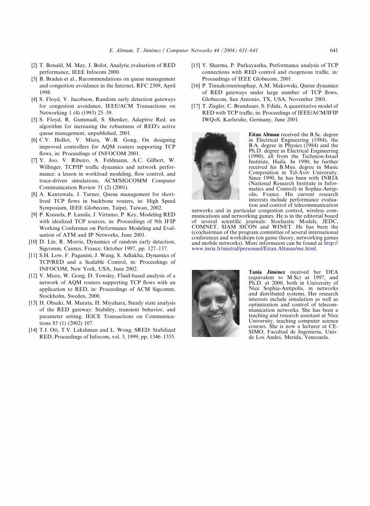
Fig. 24. Window size evolution (y-axis) of a connection that
suffered many losses for gentle RED in light load as a function
of time (x-axis).
0
5
10
15
20
25
30
35
40
45
50
150 152 154 156 158 160
average queue sizeinstantaneous size
Fig. 26. Average and instantaneous queue size (y-axis) for
gentle RED as a function of time (x-axis), bottleneck link of 2.5
Mbps.
640 E. Altman, T. Jim�enez / Computer Networks 44 (2004) 631–641
smoothes the traffic. This smoother increase in
window size due to earlier losses finally results in
less losses in the overall transfer. To understand
this better, we plot the evolution of the queue size
and RED�s average queue size for both cases in
Figs. 25 and 26. We see that out transfer caused apeak in the instantaneous queue size at time 153 s
approximately that resulted in a queue overflow;
this occurred in both cases. However, we see that
the average queue size is larger for the heavy load
case, which resulted in drops occurring earlier due
to RED early discarding. This explains the more
smooth behavior of the transmission at heavy
load, and thus its better performance in terms oflosses. This type of phenomenon can also explain
0
5
10
15
20
25
30
35
40
45
50
150 152 154 156 158 160
average queue sizeinstantaneous size
Fig. 25. Average and instantaneous queue size (y-axis) for
gentle RED as a function of time (x-axis), bottleneck link of 2.5
Mbps.
the strange behavior we observed in Section 3,
where in some cases, the number of active sessions
was larger for the lighter load than for the larger
one.
7. Conclusions
We examined how loss rate of a transfer and the
transfer throughput are related to its size. We have
seen that RED is biased against long connections
in terms of loss probabilities but that this bias
decreases as the load increases. In terms of
throughput, RED is fairer than in terms of the lossrate. Best performance has been obtained with
gentle RED, and in general all variants of RED
performed better than drop-tail.
In our simulation scenarios, file transfers could
be identified with bursts. For example, ‘‘spikes’’ in
Figs. 25 and 26 correspond to file transfers. In that
case, fairness in terms of the size of a file can be
identified with fairness in terms of burst size. Ourconclusions on fairness in terms of burst size are
then different than those that had been obtained in
previous work through simulations of permanent
connections.
References
[1] A. Arvidsson, P. Karlsson, On traffic models for TCP/IP,
in: Proceedings of 16th International Teletraffic Congress
(ITC16), Edinburgh, UK, June 1999.
E. Altman, T. Jim�enez / Computer Networks 44 (2004) 631–641 641
[2] T. Bonald, M. May, J. Bolot, Analytic evaluation of RED
performance, IEEE Infocom 2000.
[3] B. Braden et al., Recommendations on queue management
and congestion avoidance in the Internet, RFC 2309, April
1998.
[4] S. Floyd, V. Jacobson, Random early detection gateways
for congestion avoidance, IEEE/ACM Transactions on
Networking 1 (4) (1993) 25–39.
[5] S. Floyd, R. Gummadi, S. Shenker, Adaptive Red: an
algorithm for increasing the robustness of RED�s active
queue management, unpublished, 2001.
[6] C.V. Hollot, V. Misra, W.-B. Gong, On designing
improved controllers for AQM routers supporting TCP
flows, in: Proceedings of INFOCOM 2001.
[7] Y. Joo, V. Ribeiro, A. Feldmann, A.C. Gilbert, W.
Willinger, TCP/IP traffic dynamics and network perfor-
mance: a lesson in workload modeling, flow control, and
trace-driven simulations, ACM/SIGCOMM Computer
Communication Review 31 (2) (2001).
[8] A. Kantawala, J. Turner, Queue management for short-
lived TCP flows in backbone routers, in: High Speed
Symposium, IEEE Globecom, Taipei, Taiwan, 2002.
[9] P. Kuusela, P. Lassila, J. Virtamo, P. Key, Modeling RED
with idealized TCP sources, in: Proceedings of 9th IFIP
Working Conference on Performance Modeling and Eval-
uation of ATM and IP Networks, June 2001.
[10] D. Lin, R. Morris, Dynamics of random early detection,
Sigcomm, Cannes, France, October 1997, pp. 127–137.
[11] S.H. Low, F. Paganini, J. Wang, S. Adlakha, Dynamics of
TCP/RED and a Scalable Control, in: Proceedings of
INFOCOM, New York, USA, June 2002.
[12] V. Misra, W. Gong, D. Towsley, Fluid-based analysis of a
network of AQM routers supporting TCP flows with an
application to RED, in: Proceedings of ACM Sigcomm,
Stockholm, Sweden, 2000.
[13] H. Ohsaki, M. Murata, H. Miyahara, Steady state analysis
of the RED gateway: Stability, transient behavior, and
parameter setting, IEICE Transactions on Communica-
tions 85 (1) (2002) 107.
[14] T.J. Ott, T.V. Lakshman and L. Wong, SRED: Stabilized
RED, Proceedings of Infocom, vol. 3, 1999, pp. 1346–1355.
[15] V. Sharma, P. Purkayastha, Performance analysis of TCP
connections with RED control and exogenous traffic, in:
Proceedings of IEEE Globecom, 2001.
[16] P. Tinnakornsrisuphap, A.M. Makowski, Queue dynamics
of RED gateways under large number of TCP flows,
Globecom, San Antonio, TX, USA, November 2001.
[17] T. Ziegler, C. Brandauer, S. Fdida, A quantitative model of
RED with TCP traffic, in: Proceedings of IEEE/ACM/IFIP
IWQoS, Karlsruhe, Germany, June 2001.
Eitan Altman received the B.Sc. degreein Electrical Engineering (1984), theB.A. degree in Physics (1984) and thePh.D. degree in Electrical Engineering(1990), all from the Technion-IsraelInstitute, Haifa. In 1990, he furtherreceived his B.Mus. degree in MusicComposition in Tel-Aviv University.Since 1990, he has been with INRIA(National Research Institute in Infor-matics and Control) in Sophia-Antip-olis, France. His current researchinterests include performance evalua-tion and control of telecommunication
networks and in particular congestion control, wireless com-munications and networking games. He is in the editorial boardof several scientific journals: Stochastic Models, JEDC,COMNET, SIAM SICON and WINET. He has been the(co)chairman of the program committee of several internationalconferences and workshops (on game theory, networking gamesand mobile networks). More informaion can be found at http://www.inria.fr/mistral/personnel/Eitan.Altman/me.html.
Tania Jim�enez received her DEA(equivalent to M.Sc) at 1997, andPh.D. at 2000, both in University ofNice Sophia-Antipolis, in networksand distributed systems. Her researchinterests include simulation as well asoptimization and control of telecom-munication networks. She has been ateaching and research assistant at NiceUniversity, teaching computer sciencecourses. She is now a lecturer at CE-SIMO, Facultad de Ingenieria, Univ.de Los Andes, Merida, Venezuela.


