JOURNAL OF GEOPHYSICAL RESEARCH, VOL. 104, NO. B10, PAGES 23,157-23,174, OCTOBER 10, 1999

Simulation and characterization of fracture patterns in glaciers

Anders Malthe-Sorenssen and Thomas Walmann

Department of Physics, University of Oslo, Oslo, Norway

Bjorn Jamtveit Department of Geology, University of Oslo, Oslo, Norway

Jens Feder and Totsrein Jossang Department of Physics, University of Oslo, Oslo, Norway

Abstract. During drainage of subglacial lakes the surface of the glacier subsides and fractures, generating a homogeneous, circular fracture pattern on the rim of the resulting depression. We have analyzed several fracture patterns around the Skafta cauldron on Iceland. A regular fracture spacing was observed on the cauldron rim, indicating that the region was subjected to a uniform strain. In this region, standard image analysis techniques were applied to find the lengths L and open areas A of the fractures. We demonstrate that an understanding of sampling biases allows a scaling relation L cr A • to be established and the exponent/• to be determined. This relation provides a quantitative characterization of interactions between fractures in the population. The value of • is higher for that observed for laboratory experiments on clay, but the uncertainties do not rule out a universal behavior, which applies to ice, rock, and all other solids. The size distribution of fractures did not display a similarly simple crossover behavior, and a power law scaling relation could not be established without a better understanding of the crossovers for large fractures. We introduce a simple simulation model that reproduces the most important visual and statistical properties of the glacier fracture pattern. The direct comparison validates the use of the model to simulate geological fracturing processes.

1. Introduction

Circular fractures are observed in many naturally oc- curring fracture patterns, spanning a wide range of phe- nomena and materials from drainage cauldrons above subglacial lakes [Bjb'rnsson, 1975], rock calderas [An- derson, 1936], salt domes [Ramberg, 1981], volcanoes [Gudmundsson, 1997], and coronae on Venus [Smrekar and $tofan, 1997]. The recurring circular symmetry arises from similarities in geometry and deformation history. There are also strong visual similarities be- tween fracture patterns from different geometries and deformation histories: The circular fracture patterns observed after subglacial drainage events are similar to fracture patterns observed in laboratory experiments on clay [Oertel, 1965] and sand [Walmann et al., 1996], and in faulting of rocks [Ramsay and Huber,

Copyright 1999 by the American Geophysical Union.

Paper number 1999JB900219. 0148-0227/99 / 1999 J B 900219509.00

1987]. This indicates that there are statistical similar- ities between the fracture patterns. However, reliable quantitative measures that characterize the similarities have only been developed to a small degree. Given reliable statistical measures, numerical models of the fracture process can be constructed and constrained by field studies and laboratory-scale experiments for par- ticular, well-defined deformation histories and geome- tries. A constrained model can then be applied to more complicated scenarios both to predict the occurrence of fractures and to improve the understanding of fracture processes. In particular, numerical models can be used to determine the relationship between the fracture pat- tern and deformation history, geometry, and material properties. In this study we characterize the fracture patterns in glaciers after drainage of subglacial lakes, develop a simple simulation model of the process, and constrain the model by statistical and visual compar- isons with the glacier patterns.

The similar appearance of fracture patterns from dif- ferent sources depends both on the statistical similar- ity of the shapes of individual fractures and on sim-

23,157

23,158 MALTHE-SORENSSEN ET AL.: FRACTURE PATTERNS IN GLACIERS

ilarities in the spatial distribution of fractures. It is now well established that the surface of an individual fracture can be described as a self-affine fractal sur-

face [Bouchaud, 1997], but a corresponding consensus has not been achieved for fracture patterns. Attempts have been made to characterize fracture patterns as self- similar fractals [Mandelbrot, 1982; $cholz and Mandel- brot, 1989], but the results are uncertain because most data sets, in particular, from geological field studies, are too small to clearly establish a self-similar scaling. The problems with a limited dynamical range are particu- larly evident for applications of box counting methods [Feder, 1988] used to describe fracture patterns with a fractal dimension, or a set of fractal dimensions. Typi- cally, an aerial map of a fracture population is divided into boxes of size a, and the number of boxes, N(a), which are intersected by fractures, is counted. For a self-similar fractal pattern [Mandelbrot, 1982] the num- ber of boxes is a power law, N(a) c• a D, where D is the fractal dimension. However, fracture patterns es- sentially consist of lines. For small boxes we therefore expect that the pattern is one-dimensional and N c• a 1. On large enough length scales the pattern is homoge- neous and two-dimensional, N c• a 2. This method also illustrates the important concept of crossovers: In or- der to establish a fractal scaling regime, a power law N c• a D must span several orders of magnitude be- tween the crossover to a 1 behavior for small a and to a 2 behavior for large a. The term crossover is here used for the case where a power law changes from one behavior, such as a D, to a different power law a I or an entirely different functional form, such as an exponential.

A characterization of fracture patterns as self-similar fractals implies that a small region of the pattern should be statistically similar to the whole pattern under an isotropic rescaling. For many fracture patterns, such as the regularly spaced fracture patterns observed in laboratory experiments on clay [Walmann et al., 1996] and in glaciers [Malthe-S•renssen et al., 1998b], this is obviously not the case. The characteristic distance be- tween fractures would change under an isotropic rescal- ing. However, the pattern might still be a self-affine fractal if the pattern is statistically invariant under a rescaling along the directions of the fractures. This is a strong statement and would require that the length, shape, and spacing of fractures must scale similarly. A somewhat weaker, but still important, characterization of the pattern would be to look for a power law dis- tribution of fracture lengths or other properties of the fracture patterns. Such a relationship would imply that some features of the fracture pattern are scale invari- ant, and it would be an important characterization of the pattern. Several studies have indeed suggested that the size distribution of fractures displays a power law scaling [Walsh and Watterson, 1987; Scholz and Man- delbrot, 1989; $cholz and Cowie, 1990]; however, the evidence is weak, and in •nany cases the distribution is clearly not consistent with a power law interpretation

[Nicol et al., 1996]. Crossovers, systematic deviations from power law behavior, appear for both small and large fractures. These have been interpreted as trunca- tion and resolution effects, but they might also depend on intrinsic length scales. Without a fundamental un- derstanding of the occurrence of crossovers, a system- atic scaling of the crossovers, or a large scaling regime between the crossovers, claims of power law behavior should not be given credibility.

Recently, a scaling relation between the fracture len- gth and the open fracture area was used to character- ize fracture patterns (fracture populations) in labora- tory experiments of uniform extension of clay [Wal- mann et al., 1996]. The experimental data implied that L c• A •, where L is the fracture length, A is the fracture area, and/• - 0.68 ß 0.02. A similar relation was found for a simple simulation model of the clay [Walmann et al., 1996; Malthe-Sorenssen et al., 1998a] and for the fracture pattern in the VatnajSkull Glacier after a re- cent drainage event [Malthe-SOrenssen et al., 1998b]. This was interpreted to imply that interactions between the fractures in the population were important, and the exponent was suggested to characterize the interactions. A similar relation has also been suggested for en eche- lon fault arrays [Vermilye and Scholz, 1995], for which the exponent is/• - 2/3. For individual, noninteracting fractures a linear relationship between throw and length is expected for any linear elastic model. This results in a square root relation between length and fracture area, /• = 1/2. Such a relation has been found in several stud- ies [Ranalii, 1977; $cholz and Cowie, 1990; Cowie and Scholz, 1992b; Scholz et al., 1993; Clark and Cox, 1996]. The behavior is, however, modified by crossovers for small and large lengths. For small lengths a crossover to a nonlinear regime was observed for the Krafia fissure swarm [Hatton et al., 1994; Renshaw and Park, 1997]. Large faults which penetrate the fracturing layer can only grow in length, and a linear behavior/• - I has been suggested [Cowie and Scholz, 1992a]. However, in order to apply such a measure to characterize a pop- ulation of interacting fractures all the fractures must be taken from a homogeneous region and subjected to a homogeneous deformation. In addition, the effects of sampling problems, a limited dynamical range, and possible crossover behaviors must be discussed in detail.

The biases and uncertainties introduced in the char-

acterization of patterns of interacting fractures are often difficult to estimate. For example, the patterns may span regions exposed to different deformations or re- gions with different material properties, the fractures may be changed by subsequent processes, such as ero- sion or later deformations, and some of the fractures might be covered or closed. The data might also be bi- ased by the method of observation or by the choice of data for analysis. If the sampling biases, such as the resolution and size of a picture of the fracture pattern, can be understood, a more precise determination of the crossover behavior is possible. As we will demonstrate,

MALTHE-SORENSSEN ET AL.: FRACTURE PATTERNS IN GLACIERS 23,159

an improved understanding of the crossovers also allows a higher precision when addressing the behavior limited by the crossovers.

The development of a numerical model to simulate fracture patterns is important in order to separate the effect of material properties, deformation history, and material geometry. Several modeling approaches have previously been used to simulate fracture patterns. Pure statistical approaches [Herrmann and Roux, 1990] de- pend directly on the statistics gathered. However, most such models have problems with including the strong spatial correlations present in fractured systems. A different approach is to model the basic physical in- teractions in the fracturing material. Recently, several models based on concepts from statistical physics have been proposed, in which the material is modeled as a network of connected elements with material prop- erties that vary locally but are homogeneous on large scales [Feng and Sen, 1984; Duxbury et al., 1987; Roux and Guyon, 1985]. Models with a similar physical ori- gin have also been used to study earthquakes, for ex- ample, spring-block models [Burridge and Knopoff, 1967; Brown et al., 1991], and to study glacier basal sliding [Fischer and Clarke, 1997; Hindmarsh, 1997]. Recently, a simple network model was used to reproduce the fracture pattern observed in experiments on clay [Walmann et al., 1996; Malthe-S•renssen et al., 1998a]. The model reproduced the most important visual and statistical properties of the clay fracture patterns. How- ever, a direct quantitative comparison between model and outcrop data has not been performed. It is there- fore important to test the model by comparing it with fracture patterns from other deformations and geome- tries and for different material properties. In addition, it is important to address whether such a simple model can be used to study deformations that are not purely two-dimensional, such as the pure extension studied in laboratory experiments on clay. The collapse cauldrons observed above drained subglacial lakes are good exam- ples of more complex, three-dimensional deformations.

One of the best geological examples of fracturing of a homogeneous material in a reasonably well defined stress field and during a single deformational event oc- curs during drainage of subglacial lakes [BjSrnsson, 1975]. The deformation and fracturing occur over a short time, and the fractures are therefore not changed by other processes or covered by snow. We have ana- lyzed the fracture patterns around the subsidence bowl in the VatnajSkul Glacier formed during drainage of a subglacial lake at Skafta, Iceland. In the outer parts of the depression (cauldron) the fracture pattern is ho- mogeneous and circular, indicating a homogeneous ra- dial straining of the top of the ice cover. We present methods for direct quantitative measurements of the shapes of the fractures in the glacier based on aerial photographs of the area. A similar analysis is performed for the fracture patterns from previous drainage events at the same site. We present a simple numerical model

based on a connected lattice of springs attached to a deformable substrate, which produces patterns that are visually and statistically similar to the glacier fractures.

This paper is organized as follows: The qualitative behavior of the glacier fracture pattern and the tech- niques of image analysis is discussed in section 2. Sec- tion 3 address the quantitative analysis of the fracture patterns. The simulation model is introduced in section 4, and the quantitative analysis and comparison with the glacier data is performed in section 5. The results from the analysis are discussed in section 6. Conclu- sions and suggestions for further studies are presented in section 7.

2. Glacier Fractures Above Drained

Subglacial Lakes

Subglacial lakes are generated by geothermal hot spots beneath the glacier. In this study we study the fracture patterns around depressions generated by the drainage of an underwater lake at Skafta, 10 km north- west of Lake GrimvStn at Iceland [BjSrnsson, 1975]. According to BjSrnsson [1975] the lake drains regu- larly at 2- to 3-year intervals. During a week a heavily crevassed circular surface depression is formed, •03 km in diameter and 150 m deep. The drainage event is a results of the constant melting underneath the glacier. The meltwater is trapped in a lake, which is sealed by the high ice overburden pressure on a rim around the depression. Eventually, the depression is reduced by inflow of ice, and a subglacial cupola of water rises un- til the seal is broken and the lake drains. Figure l a shows an aerial photo of the Skafta cauldron formed during the drainage of the subglacial lake in August 9- 21, 1996. Figure lb shows the cauldron after drainage frown July 19 to 27, 1972, and Figure lc was taken dur- ing the drainage of the lake which started on August 18 and ended the August 24, 1984.

In the central regions of the depression the deforma- tion was a complicated combination of melting, slid- ing, sinking, floating, and contact with the underlying landscape. However, farther away the surface deforma- tion appeared to be a uniform bending that produced a circular fracture pattern. The circular statistical sym- metry indicates that the glacier surface was strained radially as the center region collapsed.

In order to apply quantitative statistical methods a large ensemble of fractures exposed to a homogeneous deformation in a homogeneous material is needed. The central region in Figure l a is characterized by large de- formations and large fractures. In many places the ice has fragmented into relatively small pieces. Details such as the geometry of the underlying landscape, the water transport, and the sequence of events were important in this region. Owing to the large deformations, sin- gle fractures are also hard to discern. The central re- gion is therefore not suitable for a statistical analysis.

23,160 MALTHE-St3RENSSEN ET AL.- FRACTURE PATTERNS IN GLACIERS

Figure 1. (a) An aerial photograph of the Skafta cauldron taken on September 30, 1996. (Copyright by National Land Survey of Iceland.) The central regions are characterized by complex fracture patterns and a nonhomogeneous stress field that depends on details of the deformation. In the outer regions the fracture pattern is the result of a more uniform deformation. The picture consists of three separate photos that were scanned and joined. Consequently, the greyscale is not uniform. (b) and (c) aerial photographs of the same region taken on August 10, 1972, and August 22, 1984, respectively. (Copyright by National Land Survey of Iceland.)

However, farther from the center the fracture pattern indicates that the deformation was more uniform.

In the photos, fractures are visible due to differences in the reflection of light and appear as brighter or darker shades. A darker region corresponds to the shadow of a fracture rim, and a brighter region corresponds to a reflection from the tilted fracture surface. Only a section of the outer region was used for analysis. The

pictures were digitized using a flatbed scanner (Scan- jet 4C, Hewlett Packard) and examined digitally. The fractures were found by applying a 6 x 6 edge filter to the digital picture and setting a threshold on the in- tensity, thereby creating a binary array of pixels that corresponded to open fractures. Figure 2 shows the region used for analysis and the binary image of the fractures. The right part of the picture contained in-

MALTHE-SORENSSEN ET AL.- FRACTURE PATTERNS IN GLACIERS

Figure 2. The region indicated by-the box in Figure I was used for analysis. Fractures were found by applying an edge filter and then setting a threshold, producing Figure 2b. The right part of the picture contained intersecting, differently oriented fractures. Because intersecting fractures connect the fracture areas and therefore obscure the analysis, the region bounded by the drawn line was removed from the analysis.

23,161

tersecting fractures with a different orientation. These fractures were due to asymmetries in the stress field or other details of the glacier deformation. Since intersect- ing fractures connect the fracture areas, the geometry of the detected fractures in this region was changed. The region bounded by the drawn line was therefore re- moved from the analysis. Similarly, only outer regions of Figures la and lb were used for analysis.

3. Analysis of Glacier Fracture Patterns

A striking feature of the fracture pattern in Figure 2 is the approximately constant radial spacing between the fractures. Regular fracture spacings are well k-nown from deformations in thin layers of material attached to a deformable substrate, such as thin films of paint and thin layers of clay [Huang and Angellet, 1989; Narr and Suppe, 1991; Mandal et al., 1994]. This observa- tion therefore suggests that the glacier consists of a thin, brittle surface zone that gradually changes with depth to a more ductile material. The fracture spacing was characterized by the distance 5 between fractures mea- sured along radial lines traced at angular intervals Only fractures with an open area larger than A0 - 5 (pixels) were included in the analysis. Smaller fractures were found by the image filtering process, but these frac- tures could not be distinguished from noise from the image processing.

The distribution of fracture spacings, P(5), is shown in Figure 3. The probability density is approximately

Gaussian, with a cutoff for 5 - 0 since distances cannot be negative. A Gaussian function was fitted to the main part of the data giving an average value (5• - 18 + 1 m and a standard deviation er5 - 2.9 + 0.3 m. A local maximum in the distribution was also observed for 50 significantly smaller than (5). The distance 50 - 1.6 + 0.2 m corresponds to the typical distance between two fracture tips that are halted due to stress shielding.

Figure 4 shows the average spacing as a function of radial length r, (5)(r). The distance is approximately

0.06

0.04

0.02

0.00

0 20 40 60

•5 [m]

Figure 3. A plot of the probability density P(5) of fracture spacings 5. (The probability for the radial distance between two fractures to be in the range 5 to 5 + d5 is P(5)dS.) A fitted, Gaussian distribution is shown by the dotted line.

23,162 MALTHE-SORENSSEN ET AL' FRACTURE PATTERNS IN GLACIERS

60

40

0

0

i i i

200 400 600 800

r[m]

Figure 4. A plot of the average spacing (5) as a function of distance r measured from the rim of the region of analysis.

constant over the central region of analysis but varies significantly for large and small r. Close to the inner rim of the region of analysis (for small r), the value of <5) is smaller than for intermediate r. This indicates a larger strain in this region. For large values of r, <5) has a local maximum, which corresponds to the region with little crevassing seen in the bottom-left corner of Figure 2b. For even larger r the value of 5 decreases again. This irregular variation is probably due to inho- mogeneities in the deformation or in the material prop- erties of the glacier. In general, we expect the strain to decrease away from the center, where the bending of the cauldron decreases. This would results in the

fewer fractures and longer distances between the frac- tures. However, the plot of (5)(r) indicates that the deformation is homogeneous for intermediate value of r because (5) is approximately constant in this region. The intermediate range is therefore used in the follow- ing to estimate the statistical properties of the fracture population.

The shape of a fracture was characterized by its length and its projected area. Because the fractures were curved with an almost constant radius of curva-

ture, the arc length along the circle provided the most fundamental measure for the length. A radial center was determined from the pattern, as explained above, and the radius and angle of each point on the fracture were determined. The length L was defined as the max- imum angular deviation At) multiplied by the average radius r, L = rat). Since the fractures were short com- pared to the radius of curvature, the difference between the arc length and the end-to-end distance of a fracture was insignificant. However, for small fractures, devia- tions from a circular shape had important consequences, as will be demonstrated later. The distribution of frac-

ture lengths in the region of analysis is given by the probability density P(L) in Figure 5. We prefer to use the direct probability density and not its integral, the cumulative distribution, or the size-rank plot, because

it simplifies the discussion of crossovers, multiplicative superposition of several distributions, and sums of sev- eral different distributions. However, it introduces an uncertainty due to the binning, and the cumulative dis- tribution may be a better choice for estimating power law exponents. We have used a logarithmic binning, but a binning with a constant number of fractures in each bin did not alter the results.

The distribution P(L) has a local maximum for small values of L. This may be an effect of limited resolution but could also be due to a change in fracture mecha- nism at lower length scales. Since we cannot increase the resolution, we have no way to distinguish an intrin- sic length scale from a resolution-related cutoff. In an intermediate range over I order of magnitude, from 5 m to 100 m, the distribution is consistent with a power law P(L) oc L -•' with exponent c• - 1.4 + 0.2. For large L the distribution falls off sharply. The length at which the curve changes from approximately a straight line to a more rapidly decreasing function is called the upper crossover length Lu. The choice of Lu determines the range over which a power law should be fitted, which again determines the power law exponent c•. In order to assess whether a power law is a reasonable represen- tation of the functional form the origin of the crossover at L• must be addressed. However, L• does not nec- essarily depend on system size, as has frequently been assumed. A reduction of the size of the region of analy- sis by a factor of 2 or 4 does not change the distribution significantly, which indicates that the finite size of the region of analysis is not the only factor determining the crossover length L•. The crossover may depend on particular features of the material, the boundary con- ditions, or the deformation history. How such effects affect Lu has not been studied systematically, and the origin of the upper crossover is therefore open to spec- ulation. If there were compelling theoretical reasons to

10 0- -1

10

-2 10

10 '3

10 -4 -5

10

10 -6

o

øo o

0.1 1.0 10.0 100.0 1000.0 L [m]

Figure 5. A plot of the probability density P(L) for the fracture length L, based on 1800 fractures from the fracture pattern shown in Figure 2. The smallest fractures, which could not be discerned from noise, were removed from the analysis. The drawn line corresponds to a power law P(L) oc L -•' with exponent a - 1.4.

MALTHE-SORENSSEN ET AL.' FRACTURE PATTERNS IN GLACIERS 23,163

4O

3O

2O

10

o

o 800

' ' ' i i , , , ! , ,

i i • • • i

200 400 600

r[m]

Figure 6. A plot of the average length (L) as a function of radial distance r measured from the rim of the region of analysis.

assume a particular form for P(L), such as a power law form, the crossover length could be estimated from the data, but with such a narrow range of length scales and without a proper understanding of the crossover length we cannot distinguish the distribution from a sum of two crossover functions, one for small L and one for large L.

The average fracture length decreases away from the deformation center. Figure 6 shows a plot of the average length (L) as a function of radius r. The decrease might indicate that the radial strain decreases away from the center, consistent with the results found for the fracture spacing (5). However, a decrease in (L) may also be a result of the fractures becoming thinner farther from the center. Thinner fractures are more easily broken up into shorter fractures by the finite picture resolution.

The fractures were also characterized by their area A found from the binary image in Figure 2b. The sim- plest interpretation of A is that it corresponds to the projected area and that w = AlL corresponds to the average fault heave (the horizontal fault displacement at the surface). However, a close examination of the image reveals that the area can correspond both to the shadow from the fault and to the projected area of the fault. The filtering procedure could be tuned to single out the shadows; however, the results did not change significantly when the projected area was found. In the following, we therefore assume that the width corre- sponds to the fault heave, which is approximately pro- portional to the fault throw (the vertical displacement at the fault surface). The distribution of fracture areas, P(A), displays the same qualitative behavior as P(L), with similarly occuring crossovers. The percentage of fractured area, p(r), is an indicator of the strain in the region, and p(r) decreases slowly away from the cen- ter. This indicates that the strain decreases away from the center, and the deformation is therefore not com- pletely homogeneous. However, the strain is not linearly related to the fractured area for small strains. Conse-

quently, the variation in strain is smaller than indicated by p(r), and the homogeneity assumption remains a rea- sonable approximation.

The shapes of the fractures in the population were characterized by the relation between L and A. Fig- ure 7 shows L(A) for all fractures in Figure 2b. The lengths were averaged in logarithmic bins of A, and the estimated standard deviation for each bin is shown

by the shaded area. The curve appears to be well ap- proximated by a linear relation on a double-logarithmic plot. However, a more careful inspection reveals that the curve crosses over from one behavior for small A

(and L) to a different behavior for larger A. This can be explained as an effect of the data sampling technique. Small fractures are either not resolved at all or they ap- pear to have a constant width of about one to two pixel units. Consequently, for small L and A the observed length is proportional to the area, and a linear behav- ior L c• A is expected. For large L and A we expect, in general, a power law behavior L c• A/•. This form includes the theoretical results: •3 - 1/2, corresponding to noninteracting fractures; 3 - 2/3, corresponding to strongly interacting en echelon fractures; and /3 - 1, corresponding to fractures that only grow in length and not in width. We can therefore write the function on

the scaling form L(A) - f(A/Ao), where the area A0 is the crossover area that separates the two behaviors, and f(x) has the form

ax x (( I (1) f (x) - '

The exact form of f(x) in the crossover regime is not known, and we have no theoretical reason to prefer a particular form. However, a simple assumption is that

1000 ..................................

100

10

........

0.1 1.0 10.0 100.0 1000.0

A [m 2] Figure 7. A plot of the length L as a function of the open area A of the glacier fractures. The error bars for the logarithmic bins are shown by the shaded area. The crossover function L(A) - c•A[tanh(Ao/A)] c2 was fitted to the data using a Levenberg-Marquardt min- imization algorithm. The best fit is shown as a solid line. The crossover area Ao is indicated by the vertical dotted line.

23,164 MALTHE-SORENSSEN ET AL.' FRACTURE PATTERNS IN GLACIERS

the function has an exponential form in the crossover regime:

f(x) - cox(tanh(1)) c2 . (2) x

The full form of the crossover function is therefore

L(A) - clA(tanh(Ao/A)) • ß (3)

The constant cl is a constant scaling factor, and the constant c2 gives the power law exponent. This function has the form L(A) •_ clA for small A (A << Ao) and the form L(A) '"' clA•A 1-c• for large A (A >> Ao). The assumption of a continuous function with continuous derivatives allows the function to be fitted in the whole

crossover region, and the applicability of the crossover function can be judged from the fit. The best curve fit gives the parameters Cl - 1.77-F 0.05 m -i, Ao - 10.0-F 1.0 m 2, and c2 - 0.21 -F 0.04. The goodness-of-fit measure for this curve fitting is X • -- 1.3. The fitted function with these parameters is shown in Figure 7. The crossover length Lo, which corresponds to the area Ao, is Lo - 16.9-F 2.0 m.

For large L and A the behavior is consistent with a power law L o• A/• with/• - 0.79 4-0.04. The produced fit is significantly better than fits to a pure power law function (X• - 5.6) or a pure linear function (X• - 9.2). The crossover function was also used to test other values

of the exponent by fixing the value of c2. A fit to the be-

lOOO

lOO

lO

o.1 1.o lO.O lOO.O lOOO.O

A [m 2] Figure 9. A plot of the length L as a function of the open area A for the fractures in Figure 2. The length L was measured as the azimuthal length (circles) and as the end-to-end distance (diamonds). The curves differ only for small L and A.

sistent with/• = 1/2 over any range of fracture lengths. The crossover analysis depends on an understanding

of the scaling behavior in one of the scaling regimes. Here, the relation between length and area for small fractures was known to be linear because of the method

of data collection. This limitation of the method of

havior/• - 1/2 was also significantly poorer (X • - 4.2) observation, the finite pixel resolution, is actually an than the for the estimated value of/•. However, we advantage, since it is reflected in the scaling behavior cannot rule out the possibility that the observed results of the data. The hypothesis that the crossover length are better explained by a crossover from a linear be- depends on the pixel size can be tested by coarse grain- havior with exponent 1 to a power law behavior with ing the system. Figure 8 shows the resulting curves for exponent/• - 1/2 over a much broader range of length L(A) at different resolutions. The crossover length in- scales than the given crossover function produces, but creases as the pixel size is increased. However, the area

also changes, since a binary coarse graining is not com- with the data available the form in equation (2) is a simpler assumption. In addition, the curve is not con- pletely area preserving. For the chosen coarse graining,

for which a pixel in the coarse-grained picture was set if at least one fourth of the pixels in the coarse-graining

1000 ................................... box were set, the total fracture area increased For small fractures the scaling behavior depended on

the method used to measure the fracture length. Two measures were used, the end-to-end distance and the az-

100 imuthal length. Figure 9 shows plots of L(A) for both E measures. For large fractures the difference between the _a two methods was negligible, but for small fractures the

10 - effect of fracture irregularity was significant, and the dif- ferences became large. Consequently, the methods only differ in the region dominated by lattice effects, and the

1 ........ , .......................... measure that produced the simplest scaling behavior 1 10 100 1000 10000 was preferred. The azimuthal length corresponded very

A [m 2] closely to the length measurement used to analyze ex- tensional deformations in clay and did not include the

Figure $. A plot of the length L as a function of the effect of fracture irregularity. For small fractures the open area A for the fractures in Figure 2. The crossover length was proportional to the area, with a width given for small fractures was examined by increasing the pixel size by a coarse graining. The crossover length increases by the pixel size. For the end-to-end distance measure- systematically with increasing pixel size, as expected. ment the measured length of a fracture depended on its The plots are for coarse-graining bin sizes of 1 (circles), orientation, and a linear relation between length and 2 (diamonds), 4 (triangles), and 16 (squares) pixels. area was not observed.

MALTHE-SORENSSEN ET AL.- FRACTURE PATTERNS IN GLACIERS 23,165

0.10

0.00

-O.lO

-o.2o

-0.30

-o.4o

-o.5o

o.o

I I • i , , i ....

0.5 1.0 1.5 2.0 2.5

log(L)

A plot of the average fracture width, Figure 10. w = A/L, as a function of length L for the fractures in Figure 2. The shaded region shows the error bars estimated from the logarithmic binning.

lOOO.O

lOO.O

E 10.0

1.0

0.1

1

Figure 12.

10 100 1000 10000

A[m 2] A plot of the length L as a function of the

open area A for 10,732 fractures from Figure lb (circles) and for 9673 fractures from Figure lc (triangles). The lower curve has been shifted by a factor 4 for clarity. The error bars from a logarithmic bining are shown by the shaded areas.

The average fracture width, w = A/L, corresponds to the fault heave or the fault throw, depending on the interpretation of the measurements. Usually, faults are characterized by the maximum fault throw. However, this is due to practical problems. In field studies it is easier to measure the maximum fault throw than the av-

erage fault throw, even though the average fault throw gives a better estimate of the work during the faulting process and therefore is a more fundamental measure. Figure 10 shows a plot of the average fault width as a function of fault length for the fault population in Fig- ure 2. The behavior of w(L) can be estimated from w = A/L and the limiting behavior of L(A). For small L, L(A) cr A, and we expect w to be constant. This is consistent with the direct plot of w(L). For large L, L(A) •x A •, which implies that w e< L (1-•)/•. The plot of w(L) is not inconsistent with a such a power law be- havior, but the range of values for w is too narrow to allow a precise estimate of the exponent. Measurements based on the curve L(A) represent a better alternative

lO 0 -1

lO

-2 lO

10 -4

10-5 10-6

1 1 o 1 oo 1 ooo

L [m]

Figure 11. A plot of the probability density P(L) for the fracture length L based on patterns in Figure lb (circles) and in Figure lc (triangles).

because the dynamic range is significantly wider for the area than for the width. In addition, w is a derived quantity, and the uncertainties are large because they depend on the uncertainties in both A and L.

The fracture patterns shown in Figures lb and lc were analyzed using the same quantitative measures. Here, we concentrate on the behavior of the size distri- bution of fractures and the relationship between frac- ture length and area for the populations. The length distributions for these patterns are shown in Figure 11. The behavior is similar to that of the previously ana- lyzed population: A similar crossover appears for both small and large fractures, and no conclusions can be made about the form of this distribution. The L(A) plots in Figure 12 display a similar crossover behavior between a linear relation for small fractures to a power law behavior for large fractures. The crossover function introduced above produces reasonable fits to the curves. For large fractures the curves were consistent with a the scaling relation L --• A •. From the fitted functions the exponents were found to be /•: 0.79 + 0.05 and /• - 0.76 + 0.05 for the two patterns. The values of the exponents are close to the values observed above; how- ever, the uncertainties are larger since the data sets are smaller and contain more noise. The behavior of these

populations confirms the results and conclusions found above for the particular drainage event and suggests that the results are general features of fracture popula- tions in glaciers around drainage cauldrons of subglacial lakes.

4. Simulation of Glacier Fracture

Patterns

A numerical model based on a simple mechanical rep- resentation of the glacier surface has been used to sim- ulate the fracturing of the glacier. The glacier surface

23,166 MALTHE-SORENSSEN ET AL.: FRACTURE PATTERNS IN GLACIERS

is modeled as an interconnected network of simple me- chanical units, springs, that represent the mechanical properties of the material averaged over an intermedi- ate scale. Fracturing occurs through the irreversible removal of a spring if the stress in the spring exceeds a threshold value. The material behavior is determined

by the material properties of the springs. In the model presented here the elastic constants are not varied, and only the breaking thresholds are drawn from random distributions. The material is considered to be homoge- neous on scales much larger than the length of a spring, which is realistic for the glacier ice far from the cen- ter. On smaller scales the material is disordered, and the disorder is described by the random distribution of breaking thresholds. Several families of distributions were tested. The best results were found with a Gaus-

sian distribution with average/• and standard deviation or. The behavior of the network varies from that of a

very brittle material for small cr to a more ductile mate- rial for larger or. Changes in the elastic properties of the springs do not have any impact on the results because an equilibrium system is modeled and the magnitudes of the elastic forces are therefore inconsequential. How- ever, the behavior of the springs must be kept in a linear regime in which the forces are linearly dependent on the spring extensions.

The ice deforms and fractures at the surface as a re-

suit of the deformation and displacement of the more ductile ice deeper in the glacier. The actual form of the glacier surface and the fracture pattern depends on many factors such as the interactions between the surface and the deeper ductile ice, the melting and drainage of the meltwater and the resulting bending of the glacier, and the gravitational forces that pull the

surface down toward the center. These boundary condi- tions are not modeled in detail but are reduced to a sim-

ple set of boundary conditions: The glacier is modeled as a two-dimensional surface layer of springs attached to a deformable substrate representing the lower, duc- tile part of the glacier [Meakin, 1987; Walmann et al., 1996; Malthe-Sorenssen et al., 1998a]. The coupling ap- pears through weak springs that attach each node in the lattice to a corresponding point on the substrate, as il- lustrated in Figure 13. The deformation of the layer is controlled by the motion of the substrate and the sub- strate spring attachment points. The net force acting on a node i at a position •i is

ß -.! '-.! $

• -- Z Iqi'J(l•i -- XJ I -- di,j)?•i,j q- i•s(•ti - x i ), (4)

where the sum is over all neighboring nodes j, ffi,j is a unit vector pointing from node i to node j, •? is the position of the substrate attachment point for node i, di,j is the equilibrium distance between node i and j, ni,j is the spr!•ng constant, and no is the substrate at- tachment spring constant. The length scale d and the spring constant i•i, j can be removed from the equation by a normalization. For simplicity, we assume that both di,j -- d and Ni,j -- t• are constants. The resulting, di- mensionless equation is

• - Z (l•i - •jl - X)ffi,j + k(•i - •), (5)

where •- •'/d and the effective substrate attachment spring constant k = n0/n is the ratio of the substrate spring constant to the internode spring constant. This dimensionless equation illustrates that the equilibrium

Figure 13. The glacier is model as a triangular lattice of springs, each with the same spring constant n and equilibrium length d. Each node is connected to an underlying substrate with a spring of zero equilibrium length and a spring constant n0. The nodes and the substrate attach- ment points are in the same plane and have only been shown in separate planes for illustrational purposes.

MALTHE-SORENSSEN ET AL.: FRACTURE PATTERNS IN GLACIERS 23,167

solution does not depend on the value of n or d. The substrate attachment spring constant k localizes the propagation of the stress field and introduces a length scale. The stress field perturbation from a broken bond decays exponentially away from the broken bond with a characteristic length • • k -•/2 for small k [Malthe- $•renssen et al., 1998a]. The length is related to the average spacing between fractures normal to the direc- tion of propagation.

A simulation consists of sequence of steps, each con- sisting of a deformation followed by a lattice relation. The substrate is deformed in small steps from the initial to the final configuration. A deformation step consists both of a change in the surface geometry and of a dis- placement of the substrate attachment points along the substrate. After each deformation step the lattice is re- laxed to a position of minimal energy or, equivalently, to an equilibrium position in which the net force on each node is zero. If any bond exceeds its breaking thresh- olds after relaxation, the bond that exceeds its threshold the most is removed, and the lattice is relaxed again. The process of relaxation and bond removal is repeated until no more bonds are broken. The relaxation proce- dure follows standard overrelaxation techniques [Allen, 1954]. Because the propagation of the stress field is lo- calized by the substrate attachment, relaxation is con- siderably faster than for a network attached only at the edges.

The deformation and fracturing of the lattice is deter- mined by the geometry of the substrate and the motion of the substrate attachment points. Each point can be displaced individually, allowing many different types of deformations to be implemented. A simple example is a uniform, radial extension, which can be modeled by the following displacement of the substrate attachment point •? as a function of extension t:

= + - + (6)

where --s is the initial position of node i and •c is the Xi,o center point of the extension. This deformation does, however, not produce circular patterns. A uniform, ra- dial extension results in tensional strain in both the

radial and the azimuthal directions, which produce an isotropic extension far from the center and a radial frac- ture pattern close to the center. In order to produce circular fractures, extension must occur only in the ra- dial direction and not in the azimuthal direction. This

cannot easily be achieved in a two-dimensional plane. Consequently, we have to deform the surface in three dimensions: The lattice is forced to move along a sur- face z = f(x, y) embedded in three dimensions. A de- formation therefore consists both of a change in surface geometry and of a displacement of the substrate attach- ment points along the surface. Because the exact form of the glacier surface and the detailed deformation his- tory of the glacier are unknown, a simplified deforma- tion model was used. The surface is assumed to have a

conical form, which develops as a function of extension (simulation time) t. The height of the surface depends on the distance r - [•- •c[ to the center of the cone:

0 y) - t) - - t(r• - ro)

r•ro

ro •r•

r•r

(7)

For small r (r < r0) the surface is fiat to avoid a singu- larity that nucleates radial fractures. At large distances (r > r•) the surface is also assumed to be fiat. This re- gion corresponds to the approximately fiat region of the glacier surface far from the deformation center. The po- sitions of the substrate attachment points are found by mapping the initial positions directly onto the surface

s X s s s ) - [ y,0, y,0, t)]. (8)

As the simulation time t increases, the radial distance between neighboring substrate attachment points in- creases uniformly along the conical surface. This partic- ular deformation therefore represents a uniform, radial extension of the surface along a cone in the region be- tween r0 and r•. The radial extension is not accompa- nied by a corresponding azimuthal extension, as for the two-dime•sional radial extension. The deformation is a

strong simplification that does not capture the gradual growth of the glacier cauldron by a progressive bend- ing of the surface. However, it is a reasonable first ap- proximation that allows circular fracture patterns to be observed over an extended area subjected to the same radial extension. Consequently, it is well suited to a statistical study of the fracture pattern.

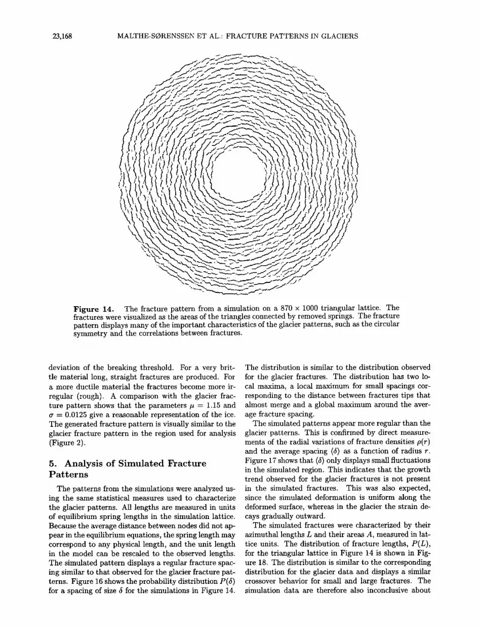
Figure 14 shows the fracture pattern from a simula- tion on a triangular lattice with a Gaussian distribu- tion of breaking threshold with average • - 1.1 and standard deviation • - 0.03. These parameters corre- spond to the distribution previously used to simulate clay [Walmann et al., 1996], but the substrate bind- ing k is stronger here. The fracture pattern is visually similar to the glacier fractures. The pattern has cir- cular symmetry, and many of the features observed in the ice are reproduced. For example, fractures start close to the ends of other fractures, and long fractures are trailed by a series of smaller fractures. However, the simulated fractures appear wider and more irreg- ular than the glacier fractures. The irregularity is an effect of the finite lattice size and the computational accuracy used, as will be discussed later.

A similar simulation was performed in a polar square lattice, for which more brittle materials can be simu- lated. The polar square lattice is a square lattice that has been bent to align the originally vertical lines with radial lines from a chosen center and the originally hor- izontal lines with azimuthal lines at a constant radial

distance from the center. Figure 15 shows patterns for different distributions of breaking thresholds. A more brittle material is produced by decreasing the standard

23,168 MALTHE-SORENSSEN ET AL.' FRACTURE PATTERNS IN GLACIERS

Figure 14. The fracture pattern from a simulation on a 870 x 1000 triangular lattice. The fractures were visualized as the areas of the triangles connected by removed springs. The fracture pattern displays many of the important characteristics of the glacier patterns, such as the circular symmetry and the correlations between fractures.

deviation of the breaking threshold. For a very brit- tle material long, straight fractures are produced. For a more ductile material the fractures become more ir-

regular (rough). A comparison with the glacier frac- ture pattern shows that the parameters • = 1.15 and • = 0.0125 give a reasonable representation of the ice. The generated fracture pattern is visually similar to the glacier fracture pattern in the region used for analysis (Figure 2).

5. Analysis of Simulated Fracture Patterns

The patterns from the simulations were analyzed us- ing the same statistical measures used to characterize the glacier patterns. All lengths are measured in units of equilibrium spring lengths in the simulation lattice. Because the average distance between nodes did not ap- pear in the equilibrium equations, the spring length may correspond to any physical length, and the unit length in the model can be rescaled to the observed lengths. The simulated pattern displays a regular fracture spac- ing similar to that observed for the glacier fracture pat- terns. Figure 16 shows the probability distribution P(5) for a spacing of size 5 for the simulations in Figure 14.

The distribution is similar to the distribution observed

for the glacier fractures. The distribution has two lo- cal maxima, a local maximum for small spacings cor- responding to the distance between fractures tips that almost merge and a global maximum around the aver- age fracture spacing.

The simulated patterns appear more regular than the glacier patterns. This is confirmed by direct measure- ments of the radial variations of fracture densities p(r) and the average spacing {5) as a function of radius r. Figure 17 shows that (5) only displays small fluctuations in the simulated region. This indicates that the growth trend observed for the glacier fractures is not present in the simulated fractures. This was also expected, since the simulated deformation is uniform along the deformed surface, whereas in the glacier the strain de- cays gradually outward.

The simulated fractures were characterized by their azimuthal lengths L and their areas A, measured in lat- tice units. The distribution of fracture lengths, P(L), for the triangular lattice in Figure 14 is shown in Fig- ure 18. The distribution is similar to the corresponding distribution for the glacier data and displays a similar crossover behavior for small and large fractures. The simulation data are therefore also inconclusive about

MALTHE-SORENSSEN ET AL.: FRACTURE PATTERNS IN GLACIERS 23,169

Figure 15. The fracture pattern from simulations on a 1051 x 250 polar, square lattice. The simulations are for different distributions of the breaking thresholds. The threshold distribution is Gaussian with an average b - 1.15. Standard deviations are (a) rr - 0.01, (b) rr - 0.0125, and (c) rr- 0.015. Figure 15b is most similar to the glacier pattern in Figure 2.

the form of the length distribution. In an intermedi- ate range, P(L) is consistent with a power law, but the range of the power law is limited by the upper crossover. It has been argued that the crossover for large L is due to the finite system size, an assertion that can be tested for the simulation model. Figure 19 shows the fracture length distribution for different system sizes/2 for sim- ulations on a triangular lattice. The upper crossover does not depend systematically on /2. The crossover might therefore depend on other characteristic length

scales, such as the characteristic fracture spacing, or on properties of the distribution of breaking thresholds. For the polar square lattice, simulations have been per- formed for several distributions of breaking thresholds. Figure 20 shows P(L, a), where rr is the standard de- viation of the width of breaking thresholds. Figure 20 shows that the upper crossover of the distribution varies systematically with rr. This indicates that the behavior of the size distribution depends on characteristic length scales associated with the brittleness of the material.

23,170 MALTHE-SORENSSEN ET AL.' FRACTURE PATTERNS IN GLACIERS

0.08 f ' , 0.06

• 0.04

0.02

0.00

0 20 40 60

Figure 16. A plot of the probability density P(5) of radial distances 5 between fractures, where 5 is mea- sured in units of the equilibrium spring length. The dis- tribution is to a good approximation Gaussian around its average value, and the corresponding Gaussian dis- tribution is shown by the dotted line.

10 o -1

10

10 '2

10_ 3

10 -4

10 -5 1 1000 lO lOO

L

Figure 18. A plot of the probability density P(L) for a fracture length L. The distribution is based on 6100 fractures from the simulation in Figure 14.

The crossover for large L in the distribution P(L) does therefore not necessarily depend on system size alone.

The effect of fracture interactions was estimated by a plot of L(A) for the simulated fractures. Figure 21 shows L(A) for the fracture population in Figure 14. The general trend of the curve is linearly increasing on the double logarithmic plot. However, systematic devi- ations can be observed. A crossover to a linear behavior, L oc A, is observed for small fractures. This is an effect of the finite lattice size, analogous to the effect of a fi- nite resolution in the photographs. For small fractures the length of a removed bond is large compared to the additional widening due to fracture propagation, and small fractures therefore appear to grow in length with- out widening. Another crossover is observed for large fractures. Owing to the substrate attachment, the per- turbation from a broken fracture is localized. Conse-

quently, the middle of a large fracture does not notice a

rupture at the fracture tip. The effect is similar to the effect of faults propagating through the crust, thereby restricting the widening of the fault but not the growth in length. The resulting behavior is L oc A. In an in- termediate region a power law behavior L oc A • can be observed; however, the range of the intermediate region is too small to allow an unambiguous estimation of the power law exponent. A power law L oc A • fitted over the whole range of length scales provides an exponent /• - 0.81+0.05. This is consistent with the behavior ob- served for the glacier patterns and indicates that on the given range of length scales the simulation model repro- duces the scaling behavior of L versus A found for the glacier patterns. From simulations of fractures in clay [Malthe-S•renssen et al., 1998a] it was found that the upper crossover length Lo, which separates the power law behavior L oc A • and the linear behavior L oc A, increases with the substrate attachment force constant

k according to L0 oc k-1/2 The scaling regime can

lO o

A

2O 10 '1

10 -2

15 • 10 '3 lO

10 -4

5 10-5 1

o

o lOO 200 300 400 Figure 19. r

Figure 17. A plot of the average spacing (5) as a function of distance r to the the deformation center for

the simulated pattern in Figure 14.

lOOO

A plot of the probability densities P(L) for the fracture length L for simulations on triangular lattices. The lattice size œ was systematically varied from œ = 1000 (solid line), œ = 600 (dashed line), œ = 300 (dotted line), to œ = 100 (dash-dotted line).

MALTHE-SORENSSEN ET AL.: FRACTURE PATTERNS IN GLACIERS 23,171

-1 lO

-2 lO

lO -4

10-5 1 10 100 1000

L

Figure 20. A plot of the probability densities P(L) for the fracture length L for simulations on a 1051 x 250 polar, square lattice. The breaking thresholds were drawn from a Gaussian distribution with average/• = 1.15 and standard deviation cr with cr: 0,01 (circles), cr = 0.0125 (diamonds), cr = 0.015 (triangles).

therefore be' systematically increased by decreasing k. However, this would also increase the average distance between fractures and would require larger systems to be simulated to retain the quality of the statistics.

A similar analysis was performed for the simulation on the polar, square lattice. The behavior is similar to the behavior observed for simulations on a triangular lattice. In particular, the results for different values of rr are indistinguishable, although the size of the largest fracture depends on the distribution, as observed for the size distribution.

6. Discussion

The model geometry represents a strong simplifica- tion of the glacier behavior. The modeled surface is conical, and the deformation is radially uniform. The glacier cauldron, on the other hand, is irregular, and the strain decays outward from the center. The defor- mation history may also differ from that portrayed in the model. In the glacier a zone of intense crevassing, and therefore of large, localized strain, moved outward when the glacier sunk down. This could be explicitly included in the model as a narrow zone of uniform ra-

dial extension that moves outward or by a nonuniform extension that decays outward. However, the present model reproduces the visual features of the glacier frac- tures, and it would therefore be difficult to determine if a more elaborate model produces even better results. We assume that a small modification of the degree of extensmn would create a small trend in the fracture

spacing and the average fracture length, as observed in the glacier, but the difference would not have a signifi- cant impact on the other statistical measures or on the visual appearance of the pattern. A very narrow bend- ing zone or a large gradient in the extension would pro-

duce fractures that are significantly more directed than the produced fractures, but such results would not be consistent with the observed behavior, which consists of fractures that are less directed than the modeled frac-

tures.

The simulation model represents the glacier as a thin layer attached to a deformable substrate. This simplifi- cation is motivated by the clearly defined average spac- ing between fractures observed in the glaciers, which confirms the picture of a thin, fracturing surface sup- ported by a deeper, ductile region. The substrate at- tachment model therefore appears to be a reasonable approximation to the coupling between the surface and the ductile bulk of the glacier. However, the glacier and the model differ in the way the geometry and strain are related. In the glacier the surface is most severely strained in regions where the surface has a small radius of curvature, whereas in the simulation model the strain is determined by the movement of the substrate attach- ment points. The maximum strain does therefore not occur at the rim of the cone, but the strain is constant along the cone and zero where the cone bends to a flat surface. In the model the surface shape serves both to provide geometrical restrictions on the movement and to produce a uniform extension. The model represents the effect of bending over an extended area but does not model that bending in detail. A more detailed model- ing of the surface bending, for which the strain and the geometry were modeled separately, could also be intro- duced but would require a more elaborate formalism without adding significantly to the understanding. The simple model presented here is a compromise which ig- nores the detailed straining history of the surface but includes the main constraining effects of the cauldron geometry and a uniform radial extension within that geometry.

Simulations on triangular lattices show that circular fractures similar to those observed in the glaciers may be produced in a general lattice that is not specifically

1000.C

100.0

10.0

1.0

0.1

1 10 100 1000 10000 A

Figure 21. A plot of the length L as a function of the open area A of the fractures from the simulation in Figure 14. The error bars from the logarithmic binning are shown by the shaded area.

23,172 MALTHE-SORENSSEN ET AL.: FRACTURE PATTERNS IN GLACIERS

adapted to the particular problem. However, for more brittle materials, that is, for smaller standard devia- tions in the breaking thresholds, simulations on triangu- lar lattices did not produce narrower and more directed fractures as expected. Instead, wiggling, sinusoidal frac- tures were observed. This is an artifact of the lattice

symmetry and the computational accuracy. Because the lattice directions do not coincide everywhere with the major stress axis, there is a competition between the main stress field and local stress field perturbations due to the discrete lattice. On small scales the fractures

have a tendency to follow the lattice directions and not the direction imposed by the stress field, in particular, for small fractures and low computational accuracies. This effect can be reduced by increasing the system size, to reduce the relative magnitude of the fluctua- tions, and by increasing the computational accuracy. These options were, however, not available with our al- gorithms because computation time t increased rapidly with both system size /2 (t oc /24) and computational accuracy.

Brittle materials could be simulated in a polar, square lattice that was oriented along the equidistance curves of the conical surface. An oriented lattice is much less

prone to fracture branching, since the lattice directions and the main stress axes coincide. In addition, a square lattice is less subject to tip branching, since a deflec- tion of the fracture tip would require a 90 ø turn away from the main stress direction. However, fractures sim- ulated in a square lattice model did not propagate only as straight lines. The merging of growing fractures con- nected neighboring tips and generated irregular, com- posite fractures. A particular feature of the square lat- tice fracture patterns is shear zones: Fracture tips tend to stop along straight lines in the fracture patterns. A similar behavior was not observed for either the trian-

gular lattice or in the glacier. This might be an ef- fect of a general problem with square lattice spring net- works: They are not stable under shear deformations. The springs can rotate without extending to relieve a shear deformation. Triangular lattices do not have this problem unless many bonds are broken. However, in the extensional deformations studied here, fracture propa- gation does not depend on the shear component of the stress field. The polar, square lattice therefore appears to be a reasonable compromise to allow simulations of brittle materials in large lattices. We emphasize that lattice adaptions to suit particular problems are not necessary; similar results can be achieved with other lattice types but represent an advantageous method to increase the efficiency of the simulations.

7. Conclusions

The fracture patterns that appear above draining subglacial lakes provide large ensembles .')f fractures from approximately homogeneous deformations in a ho- mogeneous material. The small strain gradients that

were observed did not significantly influence the frac- ture patterns and had a negligible impact on the sta- tistical characterization. These fracture populations are therefore well suited for investigations of statistical rela- tions for interacting fractures. It is important to realize that the combination of data from different fields, which might have been subjected to different deformation his- tories and also might contain different lithologies, is dangerous and, in general, cannot be trusted. It is therefore necessary to search for large fracture popula- tions from homogeneous conditions and well-controlled deformations in order to study their statistics.

The analysis of the fracture pattern was based on aerial pictures of the surface. Similar methods can be applied in many other scenarios if the fractures can be observed directly or a relief map can be produced. Stan- dard methods from image analysis can be applied to produce an image containing the open fractures. A par- ticular advantage of image analysis techniques is that the sampling biases, that is, the effect of a finite image resolution, can be estimated, and their effects can be included in the statistical analysis.

The fracture population was characterized by its spac- ing, the distribution of fracture sizes, and the scaling relation between fracture length and area. In the re- gion of analysis the glacier pattern displayed a regu- lar fracture spacing, which increased slowly with dis- tance to the cauldron center. The distribution of frac-

ture lengths did not display a convincing power law, as has frequently been claimed in other studies, but was dominated by crossovers for small and large fractures. The largest fracture was significantly smaller than the system size, and simulations indicated that the length distribution did not scale systematically as the system size was increased. This indicates that the crossover for

large lengths did not depend only on the finite sample size but also on intrinsic lengths in the system. The simulation results suggest that the intrinsic length is related to the average fracture spacing, the ductility of the material, or other details of the model. Without a better understanding of the crossover length scales a power law scaling behavior for the size distribution cannot be established. However, even if a a power law relationship is assumed to be valid, the exponent can- not be estimated without independent knowledge of the crossover behavior because the crossovers define the re-

gion over which a power law behavior is expected. This is illustrated by a direct fit of a power law function to the distribution P(L). The exponent c• in P(L) oc L -•' depends on the region over which the fit is performed.

The discussion of crossovers in the size distribution

of fractures illustrates the importance of a proper un- derstanding of crossover behaviors when scaling rela- tionships are established. For the behavior of L(A) the finite image resolution is actually an advantage because it represents a systematic error. We can therefore es- timate the behavior in the limit of small fractures. In

addition, we expect a power law behavior for large frac-

MALTHE-SORENSSEN ET AL.: FRACTURE PATTERNS IN GLACIERS 23,173

tures from theoretical considerations. This information was included in a crossover function that was fitted to

the entire data set. The crossover analysis allowed both the crossover length and the asymptotic power law ex- ponent /3 to be estimated. The analysis showed that L c• A 3 for large fractures, where/3 = 0.79 4-0.05. We emphasize that this relation characterizes the interac- tions between fracture in the whole fracture population and not the growth of individual fractures. The expo- nent /3 is larger than the exponent obtained from lab- oratory experiments on clay [Walmann et al., 1996], which suggests that different materials can be charac- terized by different exponents, but the uncertainties do not rule out a universal behavior of/3 = 2/3, corre- sponding to the behavior of strongly interacting en ech- elon fractures [ Vermilye and $cholz, 1995].

The fracture patterns produced by the simulation model display excellent visual and statistical agreement with the glacier fractures. An even better agreement was found for simulations of extensional deformations

in clay [Walmann et al., 1996]. The agreement sug- gests that there are universal features of the fracture pattern that are captured by the model and that do not depend on details of the deformation. The fracture pattern produced by the simulation model depends on the deformation history, which is explicitly included in the model. Here, motion along a three-dimensional sur- face was necessary to produce a circular fracture pat- tern. Any deformation history can be included in the model, and the model is therefore a powerful tool to study fracture patterns and to test deformation scenar- ios. However, only extensional deformations have been tested, and new features might be needed to model com- pression or shear.

Acknowledgments. We thank H. H. Hardy, Conoco, for support and enthusiasm, P. Meakin for discussions, and a referee (H. BjSrnsson) for explaining the processes behind the generation of subsidence cauldrons. This work was sup- ported by VISTA, a research corporation between the Nor- wegian Academy of Science and Letters and Den norske stats oljeselskap a.s. (STATOIL), and has received financial sup- port and a grant of computing time from the Norwegian Research Council.

References

Allen, D. M.d. G., Relaxation Methods, McGraw-Hill, New York, 1954.

Anderson, E. M., The dynamics of formation of cone sheets, ring dikes and cauldron subsidences, Proc. R. Soc. Edin- burgh, 56, 128-163, 1936.

BjSrnsson, H., Subglacial water reservoirs, jSkulhlaups and volcanic eruptions, JSkull, 25, 1-14, 1975.

Bouchaud, E., Scaling properties of cracks, J. Phys. Con- dens. Matter, 9, 4319-4344, 1997.

Brown, S. R., C. H. Scholz, and J. B. Rundle, A simpli- fied spring-block model of earthquake seismicity, Geophys. Res. Left., 18, 215-218, 1991.

Burridge, R., and L. Knopoff, Model and theoretical seis- micity, Bull. Seismol. Soc. Am., 57, 341-347, 1967.

Clark, R. M., and S. J. D. Cox, A modern regression ap- proach to determining fault displacement-length scaling relationships, J. Struct. Geol., 18, 147-152, 1996.

Cowie, P. A., and C. H. Scholz, Growth of faults by accumu- lation of seismic slip, J. Geophys. Res., 97, 11,085-11,095, 1992a.

Cowie, P. A., and C. H. Scholz, Physical expanation for the displacement-length relationship of faults using a post- yield fracture mechnics model, J. Struct. Geol., 1•, 1133- 1148, 1992b.

Duxbury, P.M., P. L. Leath, and P. D. Beale, Breakdown properties of quenched random systems: The random-fuse network, Phys. Rev. B, 36, 367-380, 1987.

l•bder, J., Fractals, Plenum, New York, 1988. Feng, $., and P. N. Sen, Percolation on elastic networks:

New exponent and threshold, Phys. Rev. Lett., 52, 216- 219, 1984.

Fischer, U. H., and G. Clarke, Stick-slip sliding behaviour at the base of a glacier, Ann. Glaciol., 2d, 390--396, 1997.

Gudmundsson, A., Stress field generating ring faults in vol- canoes, Geophys. Res. Lett., 2d, 1559-1562, 1997.

Hatton, C. G., i. G. Main, and P. G. Meredith, Non- universal scaling of fracture length and opening displace- ment, Nature, 367, 160-162, 1994.

Herrmann, H. J., and S. Roux, Statistical Models for the Fracture of Disordered Media, North-Holland, New York, 1990.

Hindmarsh, R., Deforming beds: Viscous and plastic scales of deformation, Quat. Sci. Rev., 16, 1039-1056, 1997.

Huang, Q., and J. Angelier, Fracture spacing and its relation to bed thickness, Geol. Mag., 126,355-362, 1989.

Malthe-S0renssen, A., T. Walmann, J. Feder, T. J0ssang, P. Meakin, and H. H. Hardy, Simulation of extensional fractures in clay, Phys. Rev. E, 58, 5548-5564, 1998a.

Malthe-SOrenssen, A., T. Walmann, B. Jamtveit, J. Feder, and T. JOssang, Modeling and characterization of frac- tures in the VatnajSkul Glacier, Geology, 26, 931-934, 1998b.

Mandal, N., S. K. Deb, and D. Khan, Evidence for a non- linear relationship between fracture spacing and layer thickness, J. Struct. Geol., 16, 1275-1281, 1994.

Mandelbrot, B. B., The Fractal Geometry of Nature, W. H. Freeman, New York, 1982.

Meakin, P., A simple model for elastic fracture in thin films, Thin Solid Films, 151, 165-190, 1987.

Narr, W., and J. Suppe, Joint spacing in sedimentary rocks, J. Struct. Geol., 13, 1037-1048, 1991.

Nicol, A., J. J. Walsh, J. Watterson, and P. A. Gillespie, Fault size distributions--are they really power-law?, J. Struct. Geol., 18, 191-197, 1996.

Oertel, G., The mechanism of faulting in clay experiments, Tectonophysics, 2, 343-393, 1965.

Ramberg, H., Gravity, Deformation and the Earth's Crust in Theory, Experiments, and Geological Application, 2nd ed., Academic, San Diego, Calif., 1981.

Ramsay, J. G., and M. I. Huber, The Techniques of Modern Structural Geology. v. 2, Folds and Fractures, Academic, San Diego, Calif., 1987.

Ranalii, G., Correlation between length and offset in strike- slip faults, Techtonophysics, 37, T1-T7, 1977.

Renshaw, C. E., and J. C. Park, Effect of mechanical in- teractions on the scaling of fracture length and aperture, Nature, 386,482-484, 1997.

Roux, $., and E. Guyon, Mechanical percolation: A small beam lattice study, J. Phys. Lett. Paris, d6, L999-L1005, 1985.

$cholz, C. H., and P. A. Cowie, Determination of total strain from faulting using slip measurements, Nature, 3d6,837- 839, 1990.

23,174 MALTHE-SORENSSEN ET AL.: FRACTURE PATTERNS IN GLACIERS

Scholz, C. H., and B. B. Mandelbrot, Fractals in Geophysics, Birkh&user, Basel, Switzerland, 1989.

Scholz, C. H., N.H. Dawers, J.-Z. Yu, M. H. Anders, and P. A. Cowie, Fault growth and fault scaling laws: Prelim- inary results, J. Geophys. Res., 98, 21,951-21,961, 1993.

Smrekar, S. E., and E. R. Stofan, Corona formation and heat loss on Venus by coupled upwelling and delamination, Science, 277, 1289-1294, 1997.

Vermilye, J. M., and C. H. Scholz, Relation between vein length and aperture, J. Struct. Geol., 17, 423-434, 1995.

Walmann, T., A. Malthe-S0renssen, J. Feder, T. J0ssang, P. Meakin, and H. H. Hardy, Scaling relations for the lengths and widths of fractures, Phys. Rev. Lett., 77, 5393-5396, 1996.

Walsh, J. J., and J. Watterson, Distributions of cumulative displacement and seismic slip on a single normal fault sur- face, J. Struct. Geol., 9, 1039-1046, 1987.

J. Feder, T. J0ssang, A. Malthe-S0renssen, and T. Wal- mann, Department of Physics, University of Oslo, Box 1048 Blindern, N-0316 Oslo, Norway. (e-mail: feder@fys.uio.no; jossang@fys.uio.no; malthe@fys.uio.no; walman@fys.uio.no)

B. Jamtveit, Department of Geology, University of Oslo, Box 1047 Blindern, N-0317 Oslo, Norway. (e-mail: j amt veit @ geologi. uio. no)

(Received December 30, 1998; revised May 17, 1999; accepted June 16, 1999.)