Embed Size (px)
Citation preview

Research ArticleSimulation Modeling and Analysis of Soliton WavesInteraction and Propagation in CNN Transmission Linesfor Innovative Data Communication and Processing
G Borgese1 S Vena2 P Pantano2 C Pace1 and E Bilotta2
1Dipartimento di Informatica Modellistica Elettronica e Sistemistica (DIMES) Universita della CalabriaVia P Bucci 42C 87036 Arcavacata di Rende Cosenza Italy2Dipartimento di Fisica Universita della Calabria Via P Bucci 31C 87036 Arcavacata di Rende Cosenza Italy
Correspondence should be addressed to G Borgese gianlucaborgesedimesunicalit
Received 14 February 2015 Revised 7 April 2015 Accepted 14 April 2015
Academic Editor Lu Zhen
Copyright copy 2015 G Borgese et al This is an open access article distributed under the Creative Commons Attribution Licensewhich permits unrestricted use distribution and reproduction in any medium provided the original work is properly cited
We present an innovative approach to study the interaction between oblique solitons using nonlinear transmission lines based onCellular Neural Network (CNN) paradigm A single transmission line consists of a 1D array of cells that interact with neighboringcells through both linear and nonlinear connections Each cell is controlled by a nonlinear Ordinary Differential Equation inparticular the Korteweg de Vries equation which defines the cell status and behavior Two typologies of CNN transmission linesare modelled crisscross and ring lines In order to solve KdV equations two different methods are used 4th-order Runge-Kutta andForward Euler methodsThis is done to evaluate their accuracy and stability with the purpose of implementing CNN transmissionlines on embedded systems such as FPGA andmicrocontrollers Simulationanalysis Graphic User Interface platforms are designedto conduct numerical simulations and to display elaboration results From this analysis it is possible both to identify the presenceand the propagation of soliton waves on the transmission lines and to highlight the interaction between solitons and rich nonlineardynamics With this approach it is possible to simulate and develop the transmission and processing of information within largebrain networks and high density sensor systems
1 Introduction
In the scientific literature in the last 40 years the presence ofsolitons in Nonlinear Transmission Lines (NLTL) has beenextensively studied both theoretically and experimentally [1ndash4] In the continuous case the Korteweg de Vries (KdV)equation [5] can be easily deduced by using the reductiveperturbation methods [6] It is well known that this equationhas solutions of soliton type the behavior of which has beenextensively studied both numerically [7 8] and analytically[9 10] Also some interesting related negative-order inte-grable equations including the negative-order KdV equationand some associated properties were obtained such as theresults in [11ndash13] Since the early work in NTLs [1 14 15]these solitons are still subject to studies [16ndash20] Recently thefirst robust electrical oscillator has been built the dynamicsof which is based on soliton waves [21 22]
Recent works present a completely different approach[23ndash26] based on a Cellular Neural Network (CNN) Intro-duced in 1988 by Chua and Yang [27 28] CNN consists ofa lattice of individual cells which interact with neighboringcells usually to perform very advanced sensory recognitiontasks In general the state of the CNN cells evolves in compli-ancewith nonlinearOrdinaryDifferential Equations (ODEs)and it is well known that the behavior of such systems is veryrich with striking manifestations of chaos Nonlinear ODEsdescribe a set of physical and biological phenomena funda-mental in contemporary scientific research and dynamicalsystems theory
Thenonlinear dynamics of theCNN is extremely complexand is used in contexts of real-time image processing [29]to study the emergent behaviors of complex systems (egTuring patterns) or as metamodel to simulate other math-ematical systems such as Cellular Automata (CA) [30 31]
Hindawi Publishing CorporationDiscrete Dynamics in Nature and SocietyVolume 2015 Article ID 139238 13 pageshttpdxdoiorg1011552015139238
2 Discrete Dynamics in Nature and Society
i minus 2 i minus 1 i + 1 i + 2i
Figure 1 Each cell interacts in both linear (blue lines) and nonlinear fashion (red lines) with their adjacent cells but just in a linear way withneighboring not adjacent cells
PWL PWL
i + 1 i + 2ii minus 1i minus 2
minus
minus
minus
minus minus
minusminus
minusminus
minusminus
Figure 2 CNN circuits The linear connections are made using active and passive resistances whereas non-linear connections are modeledusing non-linear piece-wise functions
CNNs can be easily implemented in hardware and thereforecapable of processing large amounts of information veryquickly and in parallel They can potentially be used to buildartificial organs such as retinas or other sensory systemsto be embodied in artificial robots to analyze vast amountsof data automatically coming from Magnetic ResonanceImaging (MRI) for patients with degenerative diseases [32]
In [33] CNN NLTL have been presented and imple-mented on FPGAThis FPGA system called DCMARK (Dis-tributed Computing Micro-ARCHitecture) allows solvingcomplex differential equations using less time than other sys-tems DCMARK uses the 1D KdV equation just as a bench-mark to evaluate and test the proper working of the systemUltimately it can produce a complex nonlinear dynamicsand show soliton waves One of the main problems in thesoliton theory is the interaction between solitons in multipledimensions [34ndash37] due to its connection with applicationFor example this problem is of fundamental importance inoptical computing [38]
This approach allows the introduction of crisscrossedtransmission lines for studying the interaction among solitonwaves Unlike traditional models based on PDEs that donot permit studying the intersection of oblique solitons thisapproach allows crossing the lines of propagation in a verysimple way and observing the behavior of solitons whenthey cross another line or when they collide with each otherThroughout this paper wewill see how this nonlinear dynam-ics is extremely rich and varied as it presents unexpected andunpredictable behaviour Such dynamics never observed inthese contexts may be useful for engineering applicationsspecifically dedicated to physical systems for transmittinginformation In this paper we deal with the followingthe general concept of CNN transmission and typologiesof NLTL investigated in Section 2 the simulationanalysissoftware environments used in Section 3 the evaluationof simulation results in Section 4 and the conclusions inSection 5
2 CNN Transmission Lines
As already introduced before a CNN transmission line canbe seen as a 1D cellular structure of119873 elements called ldquocellsrdquowhich interact through both linear and nonlinear connectionwith their adjacent cells and through only linear connectionwith the other neighbours as in Figure 1
Let us suppose that the dynamics of each cell can bemodeled through the following ODE
119906119894= 119875 (119906
119894=plusmn1) + 119871 (119906119894=plusmn2) (1)
where
119875 (119909) = 119886119909+ 1198871199092+ sdot sdot sdot (2)
is a polynomial function of 119909 and 119871(119909) = 119904119909 is a linearfunction of 119909 If we restrict our attention to polynomials ofsecond degree (1) can be written as
119906119894=
+2sum
119895=minus2119894 =119895120572119894+119895119906119894+119895+
+1sum
119895=minus1119894 =119895120573119894+1198951199062119894+119895 (3)
where120572119894+119895
(with 119895 = minus2 minus1 +1 +2)120573119894+119895
(with 119895 = minus1 +1) arecoefficients In (3)120572
119894= 120573119894= 0Assuming that120572
119894+119895and120573119894+119895
donot depend on the 119894th cell that is we consider homogeneousnetworks then (3) depends on 6 parameters 120572
minus2 120572minus1 12057211205722 120573minus1 and 1205731 representing the genome of the networkEquation (3) differs from the standard CNN because of thepresence of a reaction-diffusion term and because it is a state-controlled network
These networks can be easily implemented in hardwareFigure 2 using single-cell capacitors and resistors for activeand passive connections respectively Nonlinear connectionscan be modeled through Piecewise Linear (PWL) functions
Considering 120572minus2 = 12ℎ3 120572
minus1 = minus1ℎ3 1205721 = 1ℎ3 1205722 =
minus12ℎ3 120573minus1 = 12ℎ and 1205731 = minus12ℎ where ℎ is a constant
Discrete Dynamics in Nature and Society 3
minus1
00
0
21
34
56
7850
100
150
200
250
300
246
it
ui(t)
21
344
56
t
100
150
200
250
i
Figure 3 The initial Gaussian data decomposed into a series oflocalized travelling waves
parameter that depends on the number of cells and on thespatial interval (3) becomes
119906119894=
12ℎ3
[119906119894minus2 minus 2119906119894minus1 + 2119906119894+1 minus119906119894+2]
minus32ℎ[119906
2119894+1 minus119906
2119894minus1]
(4)
This is the spatial discretized version of 1D KdV equationIn fact (4) in the continuum limit ℎ rarr 0 approximates to thefollowing 1D KdV equation
120597119906 (119905 119909)
120597119905= minus 3120597 [119906 (119905 119909)]
2
120597119909minus1205973119906 (119905 119909)
1205971199093 (5)
Equation (4) is getting solving of Kirchhoff rsquos law as in[25]
Simulating (4) and assuming an initial function such asa Gaussian function we observe the emergence of travelingwaves as shown in Figure 3
Simulating a CNN transmission line of 300 cells andfixing properly the boundary conditions traveling solitonwaves are shown In fact as the classical solitons of theKdV equation they have very well-defined profiles with aparticular relationship between amplitude width and veloc-ity of propagation The taller and slimmer solitons travelfaster than the lower and wider ones and they maintain theirdistinctive character in the interaction with the others as itwill be explained later
If we consider 120572119894lt 0 in (4) a new linear damping term
is added In this case this equation becomes a modified KdVequation due to the presence of inhomogeneity If 120572
119894= 12119905
(4) becomes in the continuous case just the cylindrical KdVequation
Model (1) whose corresponding patterns are plotted inFigure 3 gives rise to a rich environment in which thenonlinear dynamics can be studied
On the basis of the same reasoning with some modi-fications it is possible to simulate the crisscross of two 1DCNN transmission lines analysing the interaction between
solitons belonging to different lines Even if the interactionof oblique solitons is a classic problem it is still far frombeing solved The main obstacle to its solution is that theequations at its basis are rare and no approximation seemsto be convincing The interest of researchers in this area isvery high especially in the context of optical computingbecause these studies may provide a significant input fornew forms of computation Now numerical models basedon CNN transmission lines can provide new and naturalapproaches to solve this long-standing problem
Considering two transmission lines that intersect in agiven cell (119886 119887) called cross cell as in Figure 4 the state ofeach cell except for cross cell (119886 119887) is governed by (4) Notonly does the neighborhood of cross cell (119886 119887) consist of thetwo cells at its left and right respectively but also it is made upof its upper and lower cells As before the neighboring cellsup and down have a linear excitatory synaptic connectionwhereas the other connection is nonlinear Upper or lowercells have rather inhibitory synaptic connections
Froma circuital point of view this leads to a configurationsimilar to that in Figure 5
All the cells of the two CNN transmission lines have(4) as spatial discretized state equation just at the point ofintersection between the two lines cross cell (119886 119887) is ruled bythe following spatial discretized state equation
119906119886119887=
12ℎ3
(119906119886minus2119887 minus119906119886+2119887 minus 2119906119886minus1119887 + 2119906119886+1119887)
minus32ℎ(119906
2119886+1119887 minus119906
2119886minus1119887)
+12ℎ3
(119906119886119887minus2 minus119906119886119887+2 minus 2119906119886119887minus1 + 2119906119886119887+1)
minus32ℎ(119906
2119886119887+1 minus119906
2119886119887minus1)
(6)
This equation that governs the behavior of the cross cellcould be obtained as done for (4) in [25] solving Kirchhoff rsquoslaw for the circuit in Figure 5 and finding the expression ofcurrent through the capacitor (119886 119887) The state 119906(119886 119887) of thecross cell and the voltage across the capacitor is representedby 119877 the inhibitory synaptic connection 1198771015840 the excitatorysynaptic connection and 11987710158401015840 the coefficient of the nonlinearterm Then the equation of the state of the cross cell (119886 119887)becomes
119906119886minus2119887 minus 119906119886119887
119877minus119906119886minus1119887 minus 119906119886119887
1198771015840+1199062119886minus1119887 minus 119906
2119886119887
11987710158401015840
+119906119886119887minus2 minus 119906119886119887
119877minus119906119886119887minus1 minus 119906119886119887
1198771015840+1199062119886119887minus1 minus 119906
2119886119887
11987710158401015840
=119906119886+2119887 minus 119906119886119887
119877minus119906119886+1119887 minus 119906119886119887
1198771015840+1199062119886+1119887 minus 119906
2119886119887
11987710158401015840
+119906119886119887+2 minus 119906119886119887
119877minus119906119886119887+1 minus 119906119886119887
1198771015840+1199062119886119887+1 minus 119906
2119886119887
11987710158401015840
+119862119889119906119886119887
119889119905
(7)
4 Discrete Dynamics in Nature and Society
a minus 2 b a minus 1 b a b
a b + 2
a b + 1
a b minus 1
a b minus 2
a + 1 b a + 2 b
Figure 4 Block diagram representation of the crisscrossed lines structure at the point of intersection between the two lines (red and yellowlines for nonlinear interactions blue and violet lines for linear interactions)
PWL
PWL
PWL
PWL
PWL PWL
minusminus
minusminus minus
minus minus
minus
minus
minus minus
minus
minusminus
minusminus
minusminus
minusminus
a b + 2
a b + 1
a minus 2 b a minus 1 b a b a + 1 b a + 2 b
a b minus 1
a b minus 2
Figure 5 Circuital representation of the crisscrossed lines structure at the point of intersection
Discrete Dynamics in Nature and Society 5
from which
119862119889119906119886119887
119889119905=119906119886+2119887 minus 119906119886minus2119887
119877minus119906119886+1119887 minus 119906119886minus1119887
1198771015840
+1199062119886+1119887 minus 119906
2119886minus1119887
11987710158401015840+119906119886119887+2 minus 119906119886119887minus2
119877
minus119906119886119887+1 minus 119906119886119887minus1
1198771015840+1199062119886119887+1 minus 119906
2119886119887minus1
11987710158401015840
(8)
taking 1198771015840 = 1198772 119877119862 = 2ℎ2 and 11987710158401015840119862 = 2ℎ3 where ℎ= cost and grouping together equation terms state equation(6) is obtained ℎ is a normalization parameter by which itis possible to tune the system model to improve convergenceand stability
The dynamics of cross cell is regulated by the state ofeight neighboring cells with radius 2 Neighboring cells withradius 1 interact with the state of the cell in both linear andnonlinear ways
Hence the soliton interaction is studied in two differentscenarios a ring line on which there are a single solitonpropagating and a crisscross of two lines with a soliton onboth lines The motivation for the choice of these two topo-logical setups sprang from facility for analysis and detectionof soliton dynamics In particular the second one (relatingto crisscross setup) is the best for analyzing the interactionbetween oblique solitons very useful for highlighting typicaldynamical behaviors of interaction without any complica-tions related to topology
In order to simulate the presence of a soliton we canuse as an initial condition a function such as a Gaussianfunction or a square hyperbolic secant functionwith differentmagnitudes
Considering a square hyperbolic secant function as initialcondition
119904 (119909) = 119860 sdot sech2119909 (9)
This function avoids divergence integration problemsthanks to its zero-tangent envelope for 119909 rarr plusmninfin
According to [7] if one considers the following initialcondition
119906 (119909 0) = 119901 (119901 + 1) sdot sech2119909 with 119901 gt 0 (10)
the eigenvalues of Schrodinger equation spectrum to whichevery Korteweg de Vries solution is related are
120582119899= (119901minus 119899)
2
with 119899 = 0 1 119873 (index of eigenvalue)(11)
So if 119901 is an integer number there will be the birth of119901 solitons from the initial state otherwise there will be 119901solitons with a radiation tail coming after
The magnitude of solitons is
119860119899= 2120582119899 (12)
and the velocity of propagation is
119888119899= 4120582119899= 2119860119899 (13)
As already introduced amplitude width and velocity areconnected For example amplitude is directly proportionalto velocity of propagation Higher amplitude corresponds tohigher velocity of propagation
In order to increase slightly the stability and accuracy ofForward Euler method which will be firstly validated using acustom MATLAB tool and then implemented on embeddedplatforms a particular handling is done on discretized stateequations
Starting from (4) and sorting the equation terms119873 singleequations [39] are obtained from the KdV equation
120597119906119894
120597119905=
12Δ1199093
[119906119894minus2 minus119906119894+2 + 2 (119906119894+1 minus119906119894minus1)]
+3
2Δ119909[119906
2119894minus1 minus119906
2119894+1]
(14)
where 119894 = 0 119873 is the space iteration index and Δ119909 is thespatial step of the discrete grid This numerical discretizationof spatial derivative terms of (5) has been done using a space-centered finite difference method [40]
For the time derivative term of (5) just for the firstiteration we used a forward-time finite difference method asin [7 41] because there is no preceding value at the first stepof numerical integration process obtaining (13) Hence forthe other iterations we used a centered-time finite differencemethod obtaining (14) We set 119870
1198941 = 12Δ1199093 1198701198942 = 32Δ119909
and1198701 = 1Δ1199093 1198702 = 3Δ119909
119906119896+1119894
= 119906119896
119894+Δ119905 119870
1198941 [119906119896
119894minus2 minus119906119896
119894+2 + 2 (119906119896
119894+1 minus119906119896
119894minus1)]
+1198701198942 (119906119896
119894minus12minus119906119896
119894+12)
119906119896+1119894
= 119906119896minus1119894+Δ119905 1198701 [119906
119896
119894minus2 minus119906119896
119894+2 + 2 (119906119896
119894+1 minus119906119896
119894minus1)]
+1198702 [119906119896
119894minus12minus119906119896
119894+12+119906119896
119894(119906119896
119894minus1 minus119906119896
119894+1)]
(15)
where 119896 = 0 119872 are the time iteration index 119894 = 0 119873are the spatial iteration index and Δ119905 is the integration time
The same considerations about the spatial and time dis-cretization methods have also been done for the crisscrossedlines scenario as well as the ring line scenario Starting from(6) and sorting the equation terms the spatial discretizedstate equation for the cross cell of intersection between thetwo lines is obtained
120597119906119886119887
120597119905=
12Δ1199093
[119906119886minus2119887 minus119906119886+2119887 +119906119886119887minus2 minus119906119886119887+2
+ 2 (119906119886+1119887 minus119906119886minus1119887 +119906119886119887+1 minus119906119886119887minus1)]
+3
2Δ119909[119906
2119886minus1119887 minus119906
2119886+1119887 +119906
2119886119887minus1 minus119906
2119886119887+1]
(16)
where 119886 119887 = 0 119873 are the spatial iteration index forthe two lines and Δ119909 is the space step of the discrete gridEquation (16) is the equation in which the forward-time finite
6 Discrete Dynamics in Nature and Society
Figure 6 C++ SIMANSOL GUI tool for simulation and analysis
difference method is applied while in (17) the centred-timedifference method is used for time discretization
119906119896+1119886119887
= 119906119896
119886119887+Δ119905 119870
1198941 [119906119896
119886minus2119887 minus119906119896
119886+2119887 +119906119896
119886119887minus2 minus119906119896
119886119887+2
+ 2 (119906119896119886+1119887 minus119906
119896
119886minus1119887 +119906119896
119886119887+1 minus119906119896
119886119887minus1)]
+1198701198942 [119906119896
119886minus11198872minus119906119896
119886+11198872+119906119896
119886119887minus12minus119906119896
119886119887+12]
(17)
119906119896+1119886119887
= 119906119896minus1119886119887+Δ119905 1198701 [119906
119896
119886minus2119887 minus119906119896
119886+2119887 +119906119896
119886119887minus2 minus119906119896
119886119887+2
+ 2 (119906119896119886+1119887 minus119906
119896
119886minus1119887 +119906119896
119886119887+1 minus119906119896
119886119887minus1)]
+1198702 [119906119896
119886minus11198872minus119906119896
119886+11198872+119906119896
119886119887minus12minus119906119896
119886119887+12
+119906119896
119886119887(119906119896
119886minus1119887 minus119906119896
119886+1119887 +119906119896
119886119887minus1 minus119906119896
119886119887+1)]
(18)
where 119896 = 0 119872 is the time iteration index 119886 119887 = 0 119873are the spatial iteration index for the two lines and Δ119905 is theintegration time
Using this combined approach a stable propagation of asoliton through all cells for all time cycles is obtained Thiskind of discretization is less accurate than other types but itis also the best technique in terms of implementation easinessand resources saving on embedded systems
3 SimulationAnalysisSettings and Environment
In the literature there are many numerical methods to solvestate ODEs In this work two methods are used for two dif-ferent aims a 4th-order Runge-Kutta (RK4) method in orderto conduct accurate high level analysis and a simpler For-ward Euler (FE)method to be implemented after a validationphase on embedded platforms such as FPGAs microcon-trollers DSP or ASIC FE method is chosen in order to relaxthe computing load of embedded platforms to the detrimentof accuracy and stability
With the goal of conducting extensive simulations andanalysis two Graphic User Interface (GUI) environments
Figure 7 MATLAB SIMANSOL GUI tool for simulation and anal-ysis
have been designed (SIMulation-ANalysis-SOLiton tools)The first called C++ SIMANSOL has been designed usingC++ language (Figure 6) the latter called ML SIMANSOL[42] instead has been designed in MATLAB environment(Figure 7) C++ SIMANSOL tool has been used mainlyfor fast and accurate analysis while ML-SIMANSOL toolhas been used for validation and investigation in order toverify the efficiency accuracy and stability of FE methodMATLAB is preferred to other high level languages becauseof its optimal aptitude to handle matrices and vectors easilyHaving these two high level environments allows both tocompare their respective simulation results and to validatethe ODE solving process A comparison between ForwardEuler method and Runge-Kutta method is not to show anevident difference between these two methods trivially butjust for verifying if the stability and accuracy of ForwardEuler method are acceptable using a limited number of CNNcells with respect to Runge-Kutta method The impossibilityof implementing on FPGA one 1D CNN formed by a hugenumber of computing processors (one for each cell) causesproblems of equation solution instability and divergence Soit was very important to understand the minimum numberof processors to implement on FPGA in order to minimize
Discrete Dynamics in Nature and Society 7
Table 1 Ring line simulation settings
ML-SIMANSOL 1st test 2nd test 3rd testNumber of cells (119873) 100 400 400Amplitude (119860) 2 6 12Time step (Δ119905) 001 s 000001 s 000001 sSpatial step (Δ119909) 05 005 005Number of iterations 10000 400000 400000
these problems In addition implementing a Forward Eulermethod for numerical integration permits saving a lot ofFPGA resources guaranteeing the possibility to implementlarger and larger Cellular Neural Network on the FPGA [26]allowing facing more complex dynamics problems
In the C++ SIMANSOL tool (Figure 6) there are threedifferent windows initial input function window simulationsetup window and multiwires grid setup window It is possi-ble to control all simulation parameters such as integrationmethod (Euler RK4th RK2th RK45 and RKAdaptive)boundaries (periodic zero flux and fixed) number of cellsnumber of iterations initial input function (Gaussian hyper-bolic secant sin soliton impulse etc) time step spatial stepand simulation scenario (single line crisscrossed lines andgrid network)
Instead MATLAB SIMANSOL tool (Figure 7) consists ofonly one main window from which it is possible to controlseveral simulation parameters such as number of cells num-ber of iterations soliton amplitude time step spatial stepanalysis type (time spatial or timespatial) simulation sce-nario (ring line or crisscross lines) and plot simulationresults This tool as already said implements the FE integra-tion method
Using these tools it is possible to give a complete visionand to understand complex dynamics phenomena Threetypes of graphs can be displayed a state cell variable versustime graph in which the time evolution of the state variableassociated with a certain cell of the ring line is shown astate cell variable versus space graph where the value of allstate cell variable associated with all cells is displayed fora well-defined time step a timespace graph in which thetime and space evolution of the state cell variable of all cellsis highlighted This last graph is very interesting becauseit allows getting a global vision about the propagation ofsolitons and their interaction
4 Simulation Setup and Results
41 Ring Line Analysis In the first scenario a ring lineof 100ndash400 cells is considered according to what was saidpreviously The ring-fashion feature is obtained simply byimposed periodic boundary conditions Three MATLABsimulations using the MATLAB (ML) SIMANSOL tool havebeen conducted under the following conditions (Table 1)
411 1st Test Soliton with Magnitude 2 In Figure 8 the statevariable of 10th cell in function of time (number of iterations)is shown A single soliton with magnitude 2 propagates
2
15
1
05
0
0 2000 4000 6000 8000 10000
t
u(t)
Figure 8 A single soliton with magnitude 2 which propagatesthrough the ring line in correspondence with the 10th cell
10000
9000
8000
7000
6000
5000
4000
3000
2000
1000
10 20 30 40 50 60 70 80 90 100
i
t
2181614121080604020
Figure 9 A SpaceTime graph in which a single soliton with mag-nitude 2 propagates through the ring line
through the ring line performing several loops This solitonhas a velocity of propagation of 4 according to (9) completinga single loop in about 1250 iterations or rather 125 sThere arenot any numerical instability or divergence problems duringsimulations This simulation allows verifying the quality ofForward Euler method to be used for implementation ofsoliton ring line on embedded devices [26 33]
As shown in Figure 9 the narrow parallel lines withslope of 4 represent the single soliton which performs loopsthrough the ring
As already explained in Section 2 with an amplitude of 2according to [7] just a single soliton is foreseen
412 2nd Test Soliton with Magnitude 6 This time the statecell variable of 200th cell is analysed (Figure 10) The solitonnow having an amplitude of 6 generates two solitons Henceat the 150000th iteration it is possible to see the interactionbetween the two solitons with magnitudes 8 and 2 respec-tively These two solitons come from a single soliton withinitial magnitude 6 which propagates through the ring lineThey have a velocity of propagation of 16 and 4 respectivelyThis interaction is possible because of different velocity of twosolitons
From Figure 11 it is possible to understand the velocity ofsolitons on the basis of straight linesThenarrow parallel lineswith slope of 16 represent the faster soliton withmagnitude of8 while the large line with slope of 4 represents the solitonwith magnitude of 2 In this graph the soliton interaction
8 Discrete Dynamics in Nature and Society
0
0 05 1 15 2 25 3 35 4 45
123456789
t
minus1
times105
u(t)
Figure 10 The two solitons which propagate and interact throughthe ring line in correspondence with the 200th cell
8
7
6
5
4
3
2
1
050 100 150 200 250 300 350 400
4
35
3
25
2
15
1
05
times105
t
i
Figure 11 A SpaceTime graph in which a single soliton with mag-nitude 6 propagates through the ring line and is divided into twosolitons
0
0
1 iter5000 iter10000 iter
25000 iter80000 iter
50 100 150 200 250 300 350 400
123456789
minus1
i
u(i)
Figure 12 The generation and propagation through the ring line oftwo solitons from a single soliton with magnitude 6
points are evident When there is an interaction betweensolitons it is possible to see a phase shift that is shown inthe graph as a shift of lines The slow soliton has a phase shiftlarger than fast soliton and the direction of phase shift is pos-itive for slow soliton
It is also interesting to see in Figure 12 the generation andpropagation through the ring line of the two solitons coming
002468
101214161820
05 1 15 2 25 3 35 4 45t
times105
u(t)
Figure 13 The three solitons which propagate and interact throughthe ring line in correspondence with the 150th cell
18
16
14
12
10
8
6
4
2
050
4
35
3
25
2
15
1
05
100 150 200 250 300 350 400
times105
t
i
Figure 14 A SpaceTime graph in which a single soliton with mag-nitude 12 propagates through the ring line and is divided into threesolitons
from a single soliton (blue) with magnitude 6 It is possible tosee the soliton generation at five different time iterations
413 3th Test Soliton withMagnitude 12 In this case follow-ing the time evolution of state cell variable of 150th cell moreinteractions between solitons can be seen (Figure 13) At the110000th iteration there is an interaction between the solitonwith magnitude 18 and the soliton with magnitude 2 at the150000th iteration it is possible to see the interaction betweenthe two solitons with magnitudes 8 and 2 respectively whileat the 270000th iteration we find an interaction betweensolitons with magnitudes 18 and 8 respectively These threesolitons come from a single soliton with initial magnitude 12which propagates through the ring lineThese solitons have avelocity of propagation of 36 16 and 4 respectively
Also in this case from Figure 14 it is interesting to seethe different velocity of solitons and the soliton interactionpoints The narrow parallel lines with slope of 36 representthe faster soliton with magnitude of 18 while the other lineswith slope of 16 and 4 represent the solitons with magnitudeof 2 and 8 respectively In this graph the soliton interactionpoints are evident When there is an interaction betweensolitons it is possible to see a phase shift that is shown in thegraph as a shift of lines as in the other cases seen previously
From Figure 15 the generation and propagation throughthe ring line of three solitons coming from a single soliton
Discrete Dynamics in Nature and Society 9
1 iter5000 iter10000 iter
25000 iter40000 iter
0
0
5
10
15
20
50 100 150 200 250 300 350 400i
minus5
u(i)
Figure 15 The generation and propagation through the ring line ofthree solitons from a single soliton with magnitude 12
Table 2 Simulation settings crisscross scenario
C++ SIMANSOL 1st test 2nd test 3rd testLine 119886 input Soliton None SolitonLine 119887 input Soliton Soliton Soliton (delayed)Time step (Δ119905) 00001 s 00001 s 00001 sSpatial step (Δ119909) 05 05 05Number of cells on 119886119887 lines 300 300 300Soliton magn (119860) 1 1 1ML-SIMANSOL 1st test 2nd test 3rd testLine 119886 input Soliton Soliton SolitonLine 119887 input Soliton None Soliton (delayed)Time step (Δ119905) 00001 s 00001 s 00001 sSpatial step (Δ119909) 05 05 05Number of cells on 119886119887 lines 100 100 100Soliton magn (119860) 2 2 2
(blue) with magnitude 12 are shown It is possible to see thesoliton evolution at five different time iterations as in the pre-vious cases
42 Crisscross Lines Analysis In this section some simula-tions of crisscross transmission lines are shownAlso for thesesimulations the SIMANSOL tools are used In both toolsperiodic boundary conditions are chosen building a sort ofcrossed ringsThree different types of test are conductedTheinitial conditions for these simulations are summarized inTable 2
With the C++ SIMANSOL tool solitons that propagatealong the lines before and after the crossing point are shownon the graph while using ML-SIMANSOL tool the SpaceTime graphs for lines 119886 and 119887 are plotted
421 1st Test One Soliton on Both Lines 119886 and 119887 As it canbe seen in Figures 16 and 17 two solitons belonging todifferent lines meet in the crossing point and separate again
propagating on their own line as if this interaction neverhappened After the interaction they preserve their distinc-tiveness The only observed phenomenon is the presence ofa small dispersive track and reflected solitons linked to theperiodic boundary conditions rather than to the interactionbetween the two solitons
422 2nd Test Just One Soliton on Line 119886 The secondexperiment involves the presence of a single soliton passingthrough the points of intersection between the two linesWhen the soliton reaches the point of intersection it slowsdown while on the two lines disturbances occur Aftercrossing the interaction point two new solitons emerge onefor each line it is possible to see two wave trains as well onefor each line but traveling in the opposite direction comparedto solitons as shown in Figures 18 and 19
There is also a decreasing of magnitude of the two sol-itons on line 119886 after the crossing point soliton has magni-tudes 06 on line 119886 and 05 on line 119887 for simulation with C++SIMANSOL tool while 13 and 05 respectively on averagefor simulation with ML-SIMANSOL tool The larger solitonis the one that resides on the same line as the one of theincoming soliton In addition it is possible to see phenomenaof dispersive tracks and reflected solitons too
423 3th Test One Soliton on Line 119886 and One Delayed Solitonon Line 119887 The third experiment concerns the interactionbetween two solitons of the same amplitude but phase-shifted The first soliton reaches the intersection cell beforethe other one and undergoes a process of division similarto that described in the previous experiment When thesecond soliton reaches the point of intersection it moves inan unstable environment The second soliton undergoes aprocess of division and at the end of the interaction a totalof 4 new solitons emerge Figures 20 and 21 show the secondsoliton while going through the intersection cell Again wenote that there is no symmetry between the two pairs ofsolitons On the line of the soliton which first crosses theintersection cell an emerging pair is generated which has awidth slightly larger than the second pair
The generation of two small solitons and dispersive tailson both lines is also evident
The results that emerge from this series of experimentsare extremely interesting Using both simulation tools it ispossible to see the same results even if there are numericalmismatches because of the two different integrationmethodsThey show that the interaction of oblique solitons is very richand diverse In Table 3 the results of the experiments areshown
In the first case two identical solitons interact and emergeunchanged after crossing In the second case a soliton is splitinto two smaller and different solitons In the third case twoidentical but phase-shifted solitons splits into four solitonsslightly different from each other
This kind of results even if it is still under researchcould give also some ideas about a possible utilization ofthese CNN transmission lines in terms of digital logic gatesmaking the most of their nonlinear and innovative features
10 Discrete Dynamics in Nature and Society
1080604020
a
b
minus300minus200
minus100
0
100
200
300600
500400
300200
100
0
1080604020
a
b
minus300
minus200
minus100
0
100
200
300600
500400
300200
100
0
Figure 16 Simulation with C++ SIMANSOL tool two identical solitons meet and cross with no interaction
05
15
1
2
25
3
t
times105
05
0
15
25
1
2
10 20 30 40 50 60 70 80 90 100
a
(a)
05
15
1
2
25
3
t
times105
10 20 30 40 50 60 70 80 90 100
b
05
0
15
25
1
2
(b)
Figure 17 Simulation with ML-SIMANSOL tool SpaceTime graphs for line 119886 (left) and line 119887 (right) One soliton on each line
1
05
0
ab
minus200
minus300
minus100
0
100
200
300 600500
400
300200
100
0
1
05
0
ab
minus200
minus300
minus100
0
100
200
300 600500
400
300200
100
0
Figure 18 Simulation with C++ SIMANSOL tool a soliton crossing an intersection point between two lines and divides itself into twosmaller solitons
Discrete Dynamics in Nature and Society 11
05
10 20 30 40 50 60 70 80 90 100
15
1
2
25
3
t
a
times105
05
0
15
1
2
(a)
10 20 30 40 50 60 70 80 90 100
05
15
1
2
25
3
t
b
times105
08
06
04
02
0
12
1
minus02
minus04
(b)
Figure 19 Simulation with ML-SIMANSOL tool SpaceTime graphs for line 119886 (left) and line 119887 (right) Only one soliton on line 119886
1
05
0
ab
minus300
minus400
minus200
minus100
0
100
200 600500
400
300200
100
0
(a)
1
05
0
ab
600500
400
300200
100
0minus300
minus400
minus200
minus100
0
100
200
(b)
Figure 20 Simulation with C++ SIMANSOL tool solitons (one on line 119887with a negative delay) before and after they crossed the intersectioncell
Table 3 Results table crisscross scenario
C++ SIMANSOL 1st test 2nd test 3rd testLine 119886 input Soliton (119860 = 1) None Soliton (119860 = 1)Line 119887 input Soliton (119860 = 1) Soliton (119860 = 1) Soliton (delayed)Line 119886 output Soliton (119860 = 1) Soliton (119860 = 05) Two solitons (119860 = 04 03)Line 119887 output Soliton (119860 = 1) Soliton (119860 = 06) Two solitons (119860 = 04 03)ML-SIMANSOL 1st test 2nd test 3rd testLine 119886 input Soliton (119860 = 2) Soliton (119860 = 2) Soliton (119860 = 2)Line 119887 input Soliton (119860 = 2) None Soliton (delayed)Line 119886 output Soliton (119860 = 2) Soliton (119860 = 13) Two solitons (119860 = 14 07)Line 119887 output Soliton (119860 = 2) Soliton (119860 = 05) Two solitons (119860 = 14 07)
12 Discrete Dynamics in Nature and Society
05
15
1
2
05
0
15
1
2
25
3
t
times105
minus05
10 20 30 40 50 60 70 80 90 100
a
(a)
05
15
1
2
25
3
t
times105
05
0
15
25
1
2
minus05
10 20 30 40 50 60 70 80 90 100
b
(b)
Figure 21 Simulation with ML-SIMANSOL tool SpaceTime graphs for line 119886 (left) and line 119887 (right) One soliton on line 119886 and one solitonwith a negative spatial delay of 25 cells on line 119887
5 Conclusions
In this work a new approach to the transmission lines basedon nonlinear CNN is presented After providing the basicequation that governs the status of each cell the presenceand the interaction of solitary waves have been detectedThese waves interact with each other while maintaining theirdistinctivenessThis behavior is not surprising because in thecase where the network is continuous the equation of statejust becomes the well-known KdV equation The introduc-tion of nonhomogeneous terms provides a new approach tothe study of wave propagation inmultidimensional nonlinearand dispersive media Furthermore this approach allowsdealing very effectively with the problems related to inter-action between oblique solitons Several simulations in twodifferent scenarios (ring line and crisscross lines) have beenconducted with the help of two custom simulation tools Thepossibility to implement a simple Forward Euler method forsolving KdV ODE on embedded systems has been validatedThe results have great potential applications especially in theconstruction of information transmission lines embodiedinto other artificial intelligent media such as automaticexpert systems and robotic agentsThere aremany advantagesusing CNNs for designing transmission lines CNNs can beeasily implemented in silicon performing multiple processesin parallel at very high speed They constitute a very flexiblesimulation environment by which we investigate nonlineardynamics and carry out a huge number of trials with differentinitial data Using traditional systems the direct observationof solitons behavior could be very complicated Such anapproach may guarantee a technological environment fordeveloping new and unconventional forms of computationwhich exploit fully nonlinear dynamics opening interestingperspectives for the study of multidimensional solitons withreference to optical computing applications In addition this
innovative approach allows simulating neuromorphic sys-tems creating new simulation hardware for the developmentof brain-like physical agents
Conflict of Interests
The authors declare that there is no conflict of interestsregarding the publication of this paper
References
[1] R Hirota and K Suzuki ldquoTheoretical and experimental studiesof lattice solitons in nonlinear lumped networksrdquo Proceedings ofthe IEEE vol 61 no 10 pp 1483ndash1491 1973
[2] M Toda Theory of Nonlinear Lattices Original Japanese Edi-tion Springer Berlin Germany 1978
[3] K Fukushima M Wadati T Kotera K Sawada and Y Nara-hara ldquoExperimental and theoretical study of the recurrencephenomena in nonlinear transmission linerdquo Journal of thePhysical Society of Japan vol 48 no 3 pp 1029ndash1035 1980
[4] S Giambo P Pantano and P Tucci ldquoAn electrical model forKorteweg-de Vries equationrdquo American Journal of Physics vol52 pp 238ndash243 1984
[5] D J Korteweg and G de Vries ldquoXLI On the change of form oflong waves advancing in a rectangular canal and on a new typeof long stationary wavesrdquo Philosophical Magazine Series 5 vol39 no 240 pp 422ndash443 1895
[6] A M Anile J Hunter P Pantano and G Russo Ray Methodsfor Nonlinear Waves in Fluids and Plasmas Longman Scientificand Technics 1993
[7] N J Zabusky and M D Kruskal ldquoInteraction of lsquosolitonsrsquo in acollisionless plasma and the recurrence of initial statesrdquoPhysicalReview Letters vol 15 no 6 pp 240ndash243 1965
Discrete Dynamics in Nature and Society 13
[8] F Nijhoff and H Capel ldquoThe discrete Korteweg-de Vries equa-tionrdquo Acta Applicandae Mathematicae vol 39 no 1ndash3 pp 133ndash158 1995
[9] C S Gardner J M Greene M D Kruskal and R M MiuraldquoMethod for solving the Korteweg-deVries equationrdquo PhysicalReview Letters vol 19 no 19 pp 1095ndash1097 1967
[10] C S Gardner J M Greene M D Kruskal and R M MiuraldquoKorteweg-devries equation and generalizations VI methodsfor exact solutionrdquo Communications on Pure and AppliedMath-ematics vol 27 no 1 pp 97ndash133 1974
[11] Z Qiao and J Li ldquoNegative-order KdV equation with bothsolitons and kink wave solutionsrdquo Europhysics Letters vol 94no 5 Article ID 50003 2011
[12] Z Qiao and E Fan ldquoNegative-order Korteweg-de Vries equa-tionsrdquo Physical Review E vol 86 no 1 Article ID 016601 2012
[13] B Feng and Y Zhang ldquoTwo kinds of new integrable couplingsof the negative-order Korteweg-de Vries equationrdquo Advances inMathematical Physics vol 2015 Article ID 154915 8 pages 2015
[14] J Kolosick D L Landt H C S Hsuan and K E LonngrenldquoExperimental study of solitary waves in a nonlinear transmis-sion linerdquo Applied Physics vol 2 no 3 pp 129ndash131 1973
[15] R H Freeman and A E Karbowiak ldquoAn investigation ofnonlinear transmission lines and shock wavesrdquo Journal of Phys-ics D Applied Physics vol 10 no 5 pp 633ndash643 1977
[16] W-S Duan ldquoNonlinear waves propagating in the electricaltransmission linerdquo Europhysics Letters vol 66 no 2 pp 192ndash197 2004
[17] L Guardado F Benıte E Kaikina F Ruiz and M HernandezldquoAn asymptotic solution to non-linear transmission linesrdquoNon-linear Analysis Real World Applications vol 8 no 3 pp 715ndash724 2007
[18] F I I Ndzana A Mohamadou T C Kofane and L Q EnglishldquoModulated waves and pattern formation in coupled discretenonlinear LC transmission linesrdquo Physical Review E vol 78Article ID 016606 pp 1ndash13 2008
[19] S I Mostafa ldquoAnalytical study for the ability of nonlineartransmission lines to generate solitonsrdquo Chaos Solitons amp Frac-tals vol 39 no 5 pp 2125ndash2132 2009
[20] E Kengne and R Vaillancourt ldquoPropagation of solitary waveson lossy nonlinear transmission linesrdquo International Journal ofModern Physics B vol 23 no 1 pp 1ndash18 2009
[21] D S Ricketts X Li and D Ham ldquoElectrical soliton oscillatorrdquoIEEE Transactions onMicrowaveTheory and Techniques vol 54no 1 pp 373ndash382 2006
[22] T H Lee ldquoDevice physics electrical solitons come of agerdquoNature vol 440 no 7080 pp 36ndash37 2006
[23] T Roska L O Chua DWolf T Kozek R Tetzlaff and F PufferldquoSimulating nonlinear waves and partial differential equationsvia CNN I Basic techniquesrdquo IEEETransactions onCircuits andSystems I Fundamental Theory and Applications vol 42 no 10pp 807ndash815 1995
[24] L Fortuna A Rizzo and M G Xibilia ldquoModeling complexdynamics via extended PWL-based CNNsrdquo International Jour-nal of Bifurcation andChaos inApplied Sciences andEngineeringvol 13 no 11 pp 3273ndash3286 2003
[25] E Bilotta and P Pantano ldquoCellular nonlinear networks meetKdV equation a newparadigmrdquo International Journal of Bifur-cation and Chaos vol 23 no 1 Article ID 1330003 2013
[26] G Borgese C Pace P Pantano and E Bilotta ldquoFPGA-baseddistributed computing microarchitecture for complex physicaldynamics investigationrdquo IEEE Transactions on Neural Networksand Learning Systems vol 24 no 9 pp 1390ndash1399 2013
[27] LOChua andL Yang ldquoCellular neural networks theoryrdquo IEEETransactions on Circuits and Systems vol 35 no 10 pp 1257ndash1272 1988
[28] L O Chua A Paradigm for Complexity World Scientific Serieson Nonlinear Science World Scientific Singapore 1996
[29] L O Chua and T Roska Cellular Neural Networks and VisualComputing Foundations and Applications Cambridge Univer-sity Press Cambridge UK 2004
[30] E Bilotta P Pantano and S Vena ldquoArtificial micro-worldsPart I a new approach for studying life-like phenomenardquo Inter-national Journal of Bifurcation and Chaos vol 21 no 2 pp 373ndash398 2011
[31] E Bilotta and P Pantano ldquoArtificial micro-worlds part IIcellular automata growth dynamicsrdquo International Journal ofBifurcation and Chaos vol 21 no 3 pp 619ndash645 2011
[32] A Cerasa E Bilotta A Augimeri et al ldquoA cellular neural net-work methodology for the automated segmentation of multiplesclerosis lesionsrdquo Journal of Neuroscience Methods vol 203 no1 pp 193ndash199 2012
[33] G Borgese C Pace P Pantano and E Bilotta ldquoReconfigurableimplementation of a CNN-UM platform for fast dynamicalsystems simulationrdquo in Applications in Electronics PervadingIndustry Environment and Society vol 289 of Lecture Notes inElectrical Engineering Springer Berlin Germany 2014
[34] F Kako and N Yajima ldquoInteraction of ion-acoustic solitons intwo-dimensional spacerdquo Journal of the Physical Society of Japanvol 49 no 5 pp 2063ndash2071 1980
[35] J N Dinkel C Setzer S Rawal and K E Lonngren ldquoSolitonpropagation and interaction on a two-dimensional nonlineartransmission linerdquoChaos Solitons and Fractals vol 12 no 1 pp91ndash96 2001
[36] A A Alexeyev ldquoA multidimensional superposition principleclassical solitonsrdquo Physics Letters A vol 335 no 2-3 pp 197ndash206 2005
[37] T Soomere ldquoSolitons interactionsrdquo in Encyclopedia of Complex-ity and Systems Science pp 8479ndash8505 Springer NewYork NYUSA 2009
[38] B A Malomed D Mihalache F Wise and L Torner ldquoSpa-tiotemporal optical solitonsrdquo Journal of Optics B Quantum andSemiclassical Optics vol 7 no 5 pp R53ndashR72 2005
[39] L Fortuna M Frasca and A Rizzo ldquoGenerating solitons inlattices of nonlinear circuitsrdquo in Proceedings of the IEEE Inter-national Symposium on Circuits and Systems (ISCAS rsquo01) vol 2pp 680ndash683 Sydney Australia May 2001
[40] A C Vliegenthart ldquoOn finite-difference methods for the Kor-teweg-de Vries equationrdquo Journal of Engineering Mathematicsvol 5 no 2 pp 137ndash155 1971
[41] R Courant K Friedrichs and H Lewy ldquoOn the partialdifference equations of mathematical physicsrdquo IBM Journal ofResearch and Development vol 11 pp 215ndash234 1967
[42] G Borgese ldquoMATLAB SIMANSOL GUIrdquo httpesgunicalitshareMSIMANSOL GUIrar
Submit your manuscripts athttpwwwhindawicom
Hindawi Publishing Corporationhttpwwwhindawicom Volume 2014
MathematicsJournal of
Hindawi Publishing Corporationhttpwwwhindawicom Volume 2014
Mathematical Problems in Engineering
Hindawi Publishing Corporationhttpwwwhindawicom
Differential EquationsInternational Journal of
Volume 2014
Applied MathematicsJournal of
Hindawi Publishing Corporationhttpwwwhindawicom Volume 2014
Probability and StatisticsHindawi Publishing Corporationhttpwwwhindawicom Volume 2014
Journal of
Hindawi Publishing Corporationhttpwwwhindawicom Volume 2014
Mathematical PhysicsAdvances in
Complex AnalysisJournal of
Hindawi Publishing Corporationhttpwwwhindawicom Volume 2014
OptimizationJournal of
Hindawi Publishing Corporationhttpwwwhindawicom Volume 2014
CombinatoricsHindawi Publishing Corporationhttpwwwhindawicom Volume 2014
International Journal of
Hindawi Publishing Corporationhttpwwwhindawicom Volume 2014
Operations ResearchAdvances in
Journal of
Hindawi Publishing Corporationhttpwwwhindawicom Volume 2014
Function Spaces
Abstract and Applied AnalysisHindawi Publishing Corporationhttpwwwhindawicom Volume 2014
International Journal of Mathematics and Mathematical Sciences
Hindawi Publishing Corporationhttpwwwhindawicom Volume 2014
The Scientific World JournalHindawi Publishing Corporation httpwwwhindawicom Volume 2014
Hindawi Publishing Corporationhttpwwwhindawicom Volume 2014
Algebra
Discrete Dynamics in Nature and Society
Hindawi Publishing Corporationhttpwwwhindawicom Volume 2014
Hindawi Publishing Corporationhttpwwwhindawicom Volume 2014
Decision SciencesAdvances in
Discrete MathematicsJournal of
Hindawi Publishing Corporationhttpwwwhindawicom
Volume 2014 Hindawi Publishing Corporationhttpwwwhindawicom Volume 2014
Stochastic AnalysisInternational Journal of
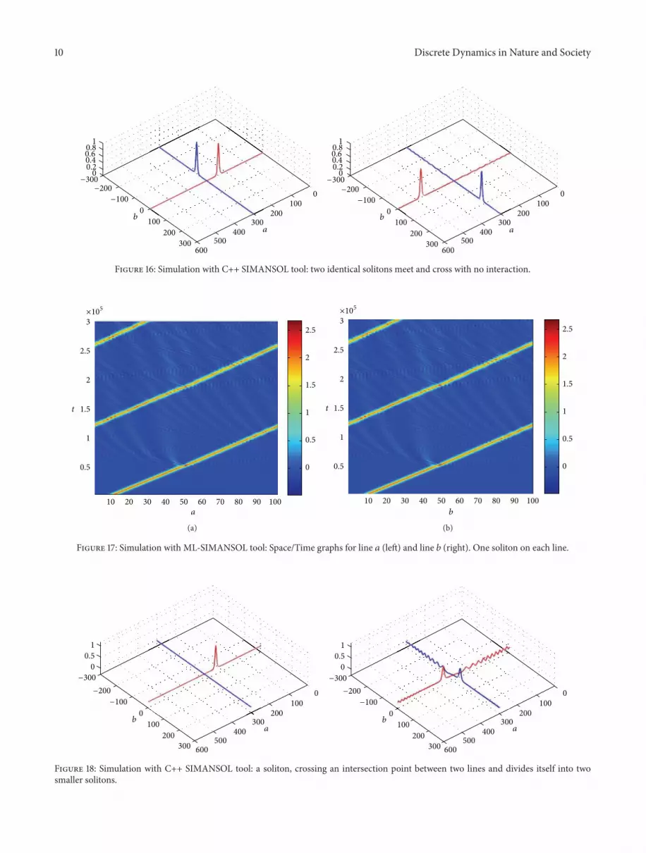
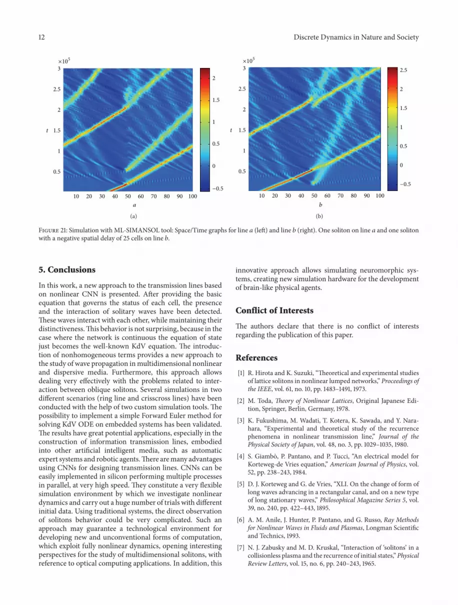


