Agricultural and Forest Meteorology, 47 (1989) 31-47 31 Elsevier Science Publishers B.V., Amsterdam - - Printed in The Netherlands

SIMULATION O F G R E E N H O U S E M I C R O C L I M A T E P R O D U C E D B Y E A R T H T U B E H E A T E X C H A N G E R S

H.J. LEVIT, R. GASPAR and R.D. PIACENTINI

Grupo de Energia Solar, Instituto de Fisica Rosario, Consejo Nacional de Investigaciones Cientificas y Tecnicas and Universidad Nacional de Rosario, Av. PeUegrini 250, (2000) Rosario (Argentina)

(Received March 10, 1988; revision accepted November 29, 1988)

ABSTRACT

Levit, H.J., Gaspar, R. and Piacentini, R.D., 1989. Simulation of greenhouse microclimate pro- duced by earth tube heat exchangers. Agric. For. Meteorol., 47: 31-47.

The conditioning system studied in this paper consists of underground pipes laid horizontally which act as "air-ground" heat exchangers. Ambient air inside the greenhouse is forced through the pipes and subsequently expelled once more into the former. The system exploits the thermal inertia of the soil whose temperature at a certain depth is virtually constant. Two models simu- lating respectively the greenhouse and the underground pipes were modified and integrated so as to simulate the operation of the system. The heat and mass balance equations that constitute the resulting model are given. With the aim of finding the optimal characteristics of the system from the technico-economic point of view, this model was used to compute the heating of a typical greenhouse in the region (Humid Pampa zone, Argentina). The results obtained for different temperature requirements are given, together with the temperature gradients of the air inside the greenhouse on a typical day in winter, both with and without the conditioning system. Finally a comparison was made between the cost of running the system and a conventional one.

INTRODUCTION

Whilst greenhouses enhance crop development by creating a microclimate, their use implies the aim of increased production and quality on the part of the producer, which consequently obliges the latter to incorporate a series of dif- ferent systems such as heating, cooling, moistening or addition of CO2, so as to achieve better air-conditioning. In Argentina, most producers adopt rudi- mentary systems: they heat by burning coal, ventilate by opening the green- houses and whitewash the coverings so as to protect them from the high degree of insolation during the summer.

Thermal conditioning systems can be divided into those which make use of conventional sources of energy (combustion or electric power) and those which

0168-1923/89/$03.50 © 1989 Elsevier Science Publishers B.V.

32

make use of new sources of energy or new technologies, such as solar, biomass, wind or geothermal energy.

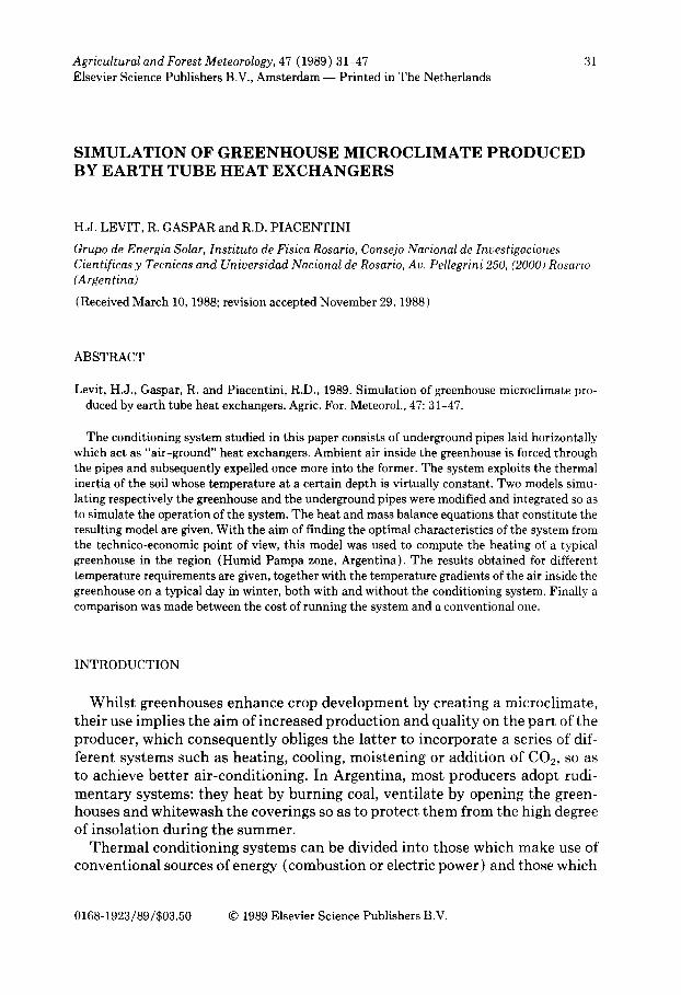
The conditioning system presented in this paper belongs to the second cat- egory, as it is based on the earth's natural conditioning capacity. Underground pipes serve as heat exchangers, heating or cooling the air, which, after having been forced through them, mixes with the air within the greenhouse in a closed circuit as shown in Fig. 1.

The use of the ground's natural potential for conditioning has been proposed and discussed by a number of authors. Peterson et al. (1975), Walker et al. (1977) and Ewen et al. (1980) studied how air discharged from mines may be used to condition greenhouses. In order for such a system to function, however, the greenhouses must necessarily be located near a mine. Kurata and Takak- ura (1985), Kozai {1985) and Mavroyanopoulus and Kyritsis (1986) sug- gested storing the excess heat accumulated during the day in the ground around the pipes so that it may be used at night when heating is required. Kurata and Takakura (1985) analysed the system using a model to simulate a single geo- metric configuration of the underground pipes concluding that by determining the heat storage and release temperatures of the pipes, the cost of the fan op- eration should also be considered, thereby implying the need for a technico- economic study of this system. Kozai (1985) and Mavroyanopoulus and Kyr- itsis (1986) discussed the heat balance by means of measurements carried out on a model similar to the above mentioned. They end their study by remarking that the heat absorbed by the system is due to natural heat storage in the subsoil from summer to winter rather than from day to night. They also show that the heat stored in the subsoil during the day represents less than 13% of the heat absorbed by the underground pipes during night for the 2 months which most need heating, thus indicating that the benefit to be derived from operating the system during the daytime is not significant.

VETI'IIATOR AND CONDITIONED AIR

GROUND

AIR INLET UNDERGROUND ETCS PIPE

Fig. 1. Perspective view of a greenhouse with underground pipe conditioning system.

33

Puri (1986, 1987) examined by the finite element formulation and the boundary element method, respectively, the behaviour of an earth tube heat exchanger. He does not however contemplate the recirculation of the air in a closed circuit; the latter is more recommendable both from the thermal and agronomical point of view.

In temperate climates, heating systems such as these are eminently suitable for use in horticultural greenhouses given that: the greenhouses only require heating for a few hours per day, and not every day during the winter months; the air temperature and the temperature inside the greenhouses without heat- ing are higher than the corresponding figures in most of the literature cited, - - in winter the average air temperature is 12.1°C whilst the average minimum for this period is 5.9 °C and the average winter temperatures at depths of 0.20 and 1 m are 12.8 and 14.5 ° C, respectively (outside greenhouse).

The above three conditions indicate that in these climates the pipes work under conditions that are different from the majority of the previously men- tioned cases.

A typical use of the heating system of around 500 h for the winter months implies that there is no risk of the thermal energy reservoir of the soil being depleted during the heating season. A daily use of approximately 8-h duration, followed by 16 h of stoppage guarantees that under a periodic regime, the power supplied by the pipes will satisfy the heating requirements.

DESCRIPTION OF EARTH TUBE CONDITIONING SYSTEM (ETCS)

It is a well-known fact that without perturbations, the temperature of"deep soil" remains virtually constant throughout the year. Furthermore, as soil pos- sesses a high thermal capacity, it constitutes a valuable heat source or heat sink. This is extremely significant when the objective is to condition enclosure naturally. The conditioning system proposed and examined in this research, the ETCS, consists of a series of underground cylindrical pipes placed horizon- tally as shown in Fig. 1. the flow rate of the air which is forced through the pipes generally ranges between 0.028 and 0.833 m 3 s- 1.

The tubes used in the ETCS can be made of any material which fits the following requirements: good heat conductor; does not deteriorate as a result of humidity or through contact with the chemical components present in the soil; capable of bearing the constant or accidental loads that will act upon them. In the present design they are connected to the interior of the greenhouse by means of manifolds at their extremities (Fig. 1 ). For practical purposes, the tube diameters vary from 0.10 to 0.40 m and their lengths from 6 to 30 m.

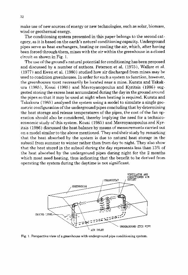
Although the ETCS can be used either for heating or for cooling, in temper- ate regions like the one studied in this paper (Humid Pampa, Argentina), only the former application is of practical interest. Table 1 shows the monthly cli-

34

TABLE 1

Month ly climatic values registered in Zavalla (33°S, 60°53 'W, 50 m above mean sea level), rep- resentat ive of the Argentine 'Pampa Humeda ' region

M o n t h Air tempera ture ( ° C) Average soil temperature ( ° C)

Average Average Average - 0 . 0 5 m - 0 . 2 0 m - 1.00 m maximum m i n i m u m

Jan. 30.9 17.1 25.2 26.4 24.8 22.8 Feb. 29.2 16.0 22.8 25.7 24.3 23.0 Mar. 26.7 14.9 20.7 22.5 22.7 22.8 Apr. 23.1 10.9 17.0 18.7 19.2 21.0 May 18.0 5.5 11.5 13.8 14.4 18.2 June 17.3 4.3 11.0 11.3 11.7 15.3 July 17.1 6.1 11.5 12.1 12.6 14.7 Aug. 17.0 5.3 11.4 11.6 11.9 14.2 Sep. 19.3 6.2 13.3 13.5 13.9 14.6 Oct. 22.9 10.9 17.2 18.3 17.6 16.3 Nov. 26.3 15.0 20.1 21.3 20.6 18.6 Dec. 28.2 14.9 21.8 23.3 23.1 21.0

matic values registered in Zavalla (33 ° S, 60 ° 53' W, 50 m above mean sea level ) representative of this region.

During the cold period, the greenhouse is kept closed and the air is recycled through the tubes. This results in a higher thermal yield since the outside air is not allowed to intervene; furthermore, the system is perfectly compatible with the use of CO2-adding devices. In this study the ETCS is not made to operate during the daytime with the greenhouse closed so as to store heat, since the general operating conditions indicate this to be inadvisable. Furthermore, as is demonstrated by Mavroyanopoulus and Kyritsis (1986), the energy stored in the ground during the day is very small compared with the magnitude of the energy that must be extracted during the night. The cost of the electricity consumed by the fans make this system unfeasible.

T H E G R E E N H O U S E - E T C S M O D E L

In order to simulate the behaviour of a greenhouse functioning with the ETCS, the mathematical model chosen must not only give an adequate de- scription of the physical processes which take place in greenhouses, but must also provide an accurate evaluation of the working of the tubes and their in- teraction with the greenhouse microclimate. With this objective in mind, the first stage of the research consisted of modifying the model used by Levit and Gaspar (1988), adding to it a subsystem which simulated the behaviour of the tubes.

35

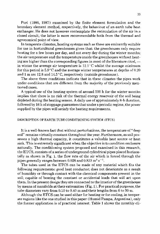
THE GREENHOUSE

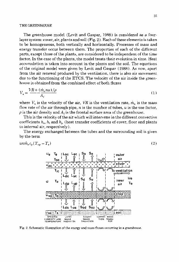
The greenhouse model (Levit and Gasper, 1988) is considered as a four- layer system: cover, air, plants and soil (Fig. 2 ). Each of these elements is taken to be homogeneous, both vertically and horizontally. Processes of mass and energy transfer occur between them. The properties of each of the different parts, except those of the plants, are considered to be independent of the time factor. In the case of the plants, the model treats their evolution in time. Heat accumulation is taken into account in the plants and the soil. The equations of the original model were given by Levit and Gaspar (1988). As now, apart from the air renewal produced by the ventilation, there is also air movement due to the functioning of the ETCS. The velocity of the air inside the green- house is obtained from the combined effect of both fluxes

V R "~- ( rna nU ) / fl Va- (1)

Af

where V~ is the velocity of the air, VR is the ventilation rate, rha is the mass flow rate of the air through pipe, n is the number of tubes, u is the use factor, p is the air density and Af is the frontal surface area of the greenhouse.

This is the velocity of the air which will intervene in the different convective coefficients h , hi and hp (heat transfer coefficients of cover, floor and plants to internal air, respectively).

The energy exchanged between the tubes and the surrounding soil is given by the term

unrna cp ( Top - T a) (2)

We Te I L o c L e c S o S e i , outer T, ~ II ~ = II 11" ; , , - a ! ! air

o c I - x / I I I v I I i ' ~ z l I = 4 + "1" + + = 4 - + + 4- + + "P "r + + - - + + "t] 4" 4 "1 - - ~ ~ - --

~o=,.4. + ~ 4. + + + +I + + 4. + -~ + 4. + + ~ c o v e r 4" . ~ w ¢ + + I + + + 4. + I + + + + + 14. + +1 + + + + + + - "~

Tc ~ ~' I I ~ Im~'vl~.~ventilation Ldc Luc M i I ? >

Ta L" L Sd Su [ I inner T: lip up II ~l" I I I air e

I v I [ ^, .

I Lds Lus ISsd Ssu I~ ~-It, ~-I . . . . . . . . . . t ............................. I . . . . . . . . . . . . . . . . . . . ' ~ 1 . [ ~ : . ' . . . . . . . . . . . . . . . . . . . .

i~s~:::: ::: ~::~s,i ~i!~ i :: i:: if:: ::i ~i:::J ~i::~::i~i::i!i::iii i~i~! i~ i~i~ ~:~i ~iii~ i~ i:::: ~i ~i~i~;~i:~i~i i i i ii~:!ii;!::::::~ ~:: ::ioj~ :ii::i::i::i~iii~i!~:~s o!:!::: i~::iiiiiii :: S P E C I F I C L O N G S H O R T C O N V E C M A S S

H U M I D I T Y A N D W A V E W A V E T I O N T R A N S T E M P E R A T U R E R A D I A T I O N R A D I A T I O N FER

Fig. 2. Schematic illustration of the energy and mass fluxes occurring in a greenhouse.

36

where Cp is the specific heat of air, Top is the temperature at the pipe outlet and is determined by resolving the model of the ETCS subsystem and Ta is the internal air temperature.

The heat balance equation of the internal air temperature, per unit of floor area, is modified from Levit and Gaspar (1988) in the following way

h~ ( Tic - Ta )-~b + hi ( Ts - Ta ) + 2hp ( Tp - Ta ) A ~ ai (3)

+hv(Te-Ta)-~ Qc ,~Sp t-unrh~cp(Top-Ta)=O Av 60Ab

where Tic is the internal cover temperature, Ac is the cover surface area, Ab is the floor area of greenhouse, Ts is the greenhouse soil temperature, Tp is the temperature of the plant leaves, Av is the floor area covered by vegetation, Lai is the leaf area index (foliage area per unit floor area), hv is the heat transfer coefficient by ventilation, Te is the temperature of the external air, Qc is the energy by convection from heaters, ~ is the latent heat of vaporization of water and Sp is the rate of spraying.

ETCS MODEL

A model of an earth tube system suited to the present study has been pre- sented by Purl (1.986), where the following assumptions were made: (i) coupled processes of heat and moisture transfer exist; (ii) the soil pressure is approximated by air pressure; (iii) the vapour-liquid interface is a function of temperature only; (iv) temperature gradients within the soil system are sufficiently small so that the total pressure is constant throughout the trans- port process; (v) the medium is macroscopically homogeneous and does not expand or contract with changing moisture content and (vi) the temperature and moisture distribution profiles in the tube vicinity are not affected either by the greenhouse or by the neighbouring tubes so that each tube has radial symmetry in temperature and soil moisture content.

Under these conditions, the equations of energy and mass balance are (Purl, 1986)

Ot-r~rtk, r~r )+ Oy\ (~y )-7-~FtplDo,vap~)-~.~y(Do,vappl~y) (4)

00 101" OT'~ O{ OTh 1 0 { 0Oh O{ 00"~

where C is the volumetric thermal capacity of the soil, T is the soil temperature, t is the time, r is the radial distance from the tube axis, ks is the thermal con- ductivity of ground, y is the axial distance from the tube inlet, Pl is the density

37

of moisture, Do,vap is the isothermal diffusivity of moisture in vapour form, 0 is the volumetric moisture content, DT is the thermal diffusivity and Do is the isothermal moisture diffusivity, with the initial conditions

O(r,y,O) =Oo(r) (6)

T(r,y,O ) =To(r) (7)

The boundary conditions for 0 are simple if it is assumed that no mass flux exists at the impervious ends in the ground.

00 =o (s)

O0 ~y(r,Lp,t) =0 (9)

where Lp is the pipe length. As regards the boundary conditions for the temperatures, if the precaution

of thermally insulating the ends is taken, there will be

O~y(r,O,t) =0 (10)

O~y(r,Lp,t) =0 (11)

At r = RL it is assumed that the values are those of the ground, independent of the existence of the pipe

T(RL,y,t) = T(RL) (12)

O(RL,y,t) = 0(RL) ( 13 )

At r= Rp

00 Or (Rp ,y,t) = 0 (impervious pipe ) ( 14 )

- k s~ (Rp ,y,t) = ht (Tap (y,t) - T(Rp,y,t) ) = - rhacp OTap

0y (15)

where RL is the arbitrarily large radial distance, Rp is the pipe radius, h t is the heat transfer coefficient from tube to air and Tap is the air temperature inside the pipe, with

T~p (0, t )= Ta(t) (16)

Two of the possible numerical solutions for the previous system of equations are as follows.

38

(i) In those cases where the variations in soil moisture are sufficiently large to affect the functioning of the tubes, the type of solution provided by Puri (1986) which uses finite elements to calculate T(r , y , t ) , O(r,y,t) and Tap(y, t ) should be used. In particular, Puri (1986) uses the TWODEPEP program de- veloped by the International Mathematical and Statistical Library (IMSL, 1983) to solve the system.

(ii) Often, where design is an important consideration, some additional sim- plifying hypotheses validated by experimental data are acceptable; the simu- lation of the system on microcomputers thus becomes a feasible option, dis- pensing with the need for more powerful computers. These hypotheses are: (a) as the radial temperature gradients in the soil in the vicinity of the tubes are significantly higher than the axial ones, the derivations on the longitudinal coordinate y may be disregarded; (b) the variation in soil moisture is incon- sequential, hence it can be assumed that 0 (r,y,t) = ct.

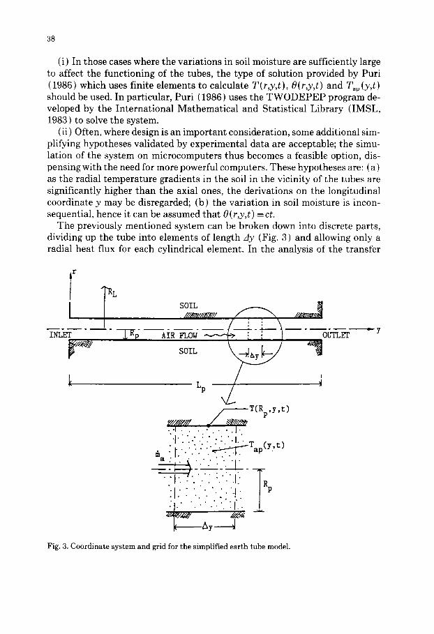
The previously mentioned system can be broken down into discrete parts, dividing up the tube into elements of length Ay (Fig. 3) and allowing only a radial heat flux for each cylindrical element. In the analysis of the transfer

r

I 7L I SOIL

IIl$/llAk~'lll

SOIL

T(Rp,y ,t)

. . i . . . - . • . . J .

' i : . - .: ." : : . - I . . : I . ' " "'"'" " ~ T a p ( y ' t )

I:: ":1. : .. . " : - I P . . . . . . . . ' . . . ' : j ' . .

OUTLET

1 - y

Fig. 3. Coordinate system and grid for the simplified earth tube model.

39

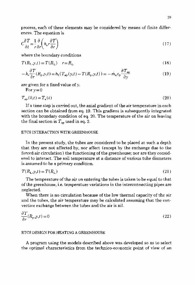
process, each of these elements may be considered by means of finite differ- ences. The equation is

cOT l O ( k s r O T ~ O t - r O r \ Or] (17)

where the boundary conditions

T(RL,y,t) =T(RL) r=RL (18)

-- k s ~ ( R p ,y,t) = ht ( Tap (y,t) - T(Rp,y,t) ) = - rhacp OTap (19) Oy

are given for a fixed value ofy. F o r y = 0

Tap (0, t)= Ta(t) (20)

If a time step is carried out, the axial gradient of the air temperature in each section can be obtained from eq. 19. This gradient is subsequently integrated with the boundary condition of eq. 20. The temperature of the air on leaving the final section is Top used in eq. 2.

ETCS INTERACTION WITH GREENHOUSE

In the present study, the tubes are considered to be placed at such a depth that they are not affected by, nor affect (except by the exchange due to the forced air circulation) the functioning of the greenhouse; nor are they consid- ered to interact. The soil temperature at a distance of various tube diameters is assumed to be a primary condition.

T(RL ,y , t )=T(RL) (21)

The temperature of the air on entering the tubes is taken to be equal to that of the greenhouse, i.e. temperature variations in the interconnecting pipes are neglected.

When there is no circulation because of the low thermal capacity of the air and the tubes, the air temperature may be calculated assuming that the con- vective exchange between the tubes and the air is nil.

~ (Rp ,y , t ) = 0 (22)

ETCS DESIGN FOR HEATING A GREENHOUSE

A program using the models described above was developed so as to select the optimal characteristics from the technico-economic point of view of an

40

TABLE 2

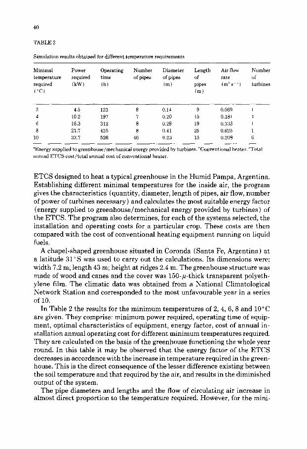
Simulation results obtained for different temperature requirements

Minimal Power Operating Number Diameter Length Air flow Number temperature required time of pipes of pipes of rate of required (kW) (h) (m) pipes (m:~s 1) turbines (°C) (m)

2 4.5 123 8 0.14 9 0.069 1 4 10.2 197 7 0.20 15 0.181 1 6 16.3 312 8 0.29 19 0.333 1 8 21.7 425 8 0.41 25 0.625 1

10 33.7 526 46 0.23 15 0.208 6

~Energy supplied to greenhouse/mechanical energy provided by turbines, bConventional heater. ~Total annual ETCS cost/total annual cost of conventional beater.

ETCS designed to heat a typical greenhouse in the Humid Pampa, Argentina. Establishing different minimal temperatures for the inside air, the program gives the characteristics (quantity, diameter, length of pipes, air flow, number of power of turbines necessary) and calculates the most suitable energy factor (energy supplied to greenhouse/mechanical energy provided by turbines) of the ETCS. The program also determines, for each of the systems selected, the installation and operating costs for a particular crop. These costs are then compared with the cost of conventional heating equipment running on liquid fuels.

A chapel-shaped greenhouse situated in Coronda (Santa Fe, Argentina) at a latitude 31°S was used to carry out the calculations. Its dimensions were: width 7.2 m; length 43 m; height at ridges 2.4 m. The greenhouse structure was made of wood and canes and the cover was 150-H-thick transparent polyeth- ylene film. The climatic data was obtained from a National Climatological Network Station and corresponded to the most unfavourable year in a series of 10.

In Table 2 the results for the minimum temperatures of 2, 4, 6, 8 and 10 o C are given. They comprise: minimum power required, operating time of equip- ment, optimal characteristics of equipment, energy factor, cost of annual in- stallation annual operating cost for different minimum temperatures required. They are calculated on the basis of the greenhouse functioning the whole year round. In this table it may be observed that the energy factor of the ETCS decreases in accordance with the increase in temperature required in the green- house. This is the direct consequence of the lesser difference existing between the soil temperature and that required by the air, and results in the diminished output of the system.

The pipe diameters and lengths and the flow of circulating air increase in almost direct proportion to the temperature required. However, for the mini-

41

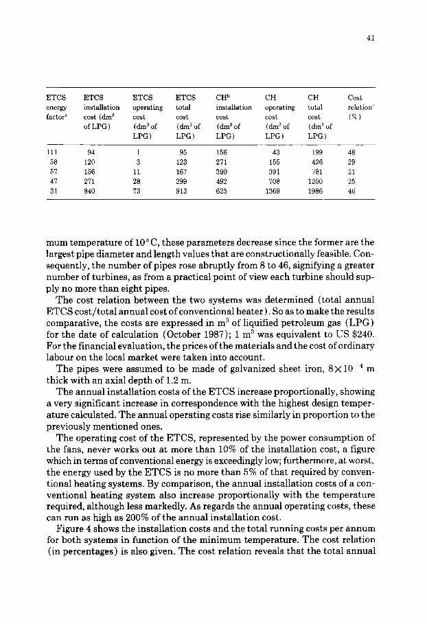
ETCS ETCS ETCS ETCS CH b CH CH

energy installation operating total installation operating total

factor a cost (dm 3 cost cost cost cost cost of LPG) (dm 3 of (din 3 of (dm 3 of (dm 3 of (dm '~ of

LPG) LPG) LPG) LPG) LPG)

Cost relation c (%)

111 94 1 95 156 43 199 48

58 120 3 123 271 155 426 29

57 156 11 167 390 391 781 21

47 271 28 299 492 708 1200 25

31 840 73 913 625 1369 1986 46

mum temperature of 10 ° C, these parameters decrease since the former are the largest pipe diameter and length values that are constructionally feasible. Con- sequently, the number of pipes rose abruptly from 8 to 46, signifying a greater number of turbines, as from a practical point of view each turbine should sup- ply no more than eight pipes.

The cost relation between the two systems was determined (total annual ETCS cost/total annual cost of conventional heater). So as to make the results comparative, the costs are expressed in m 3 of liquified petroleum gas (LPG) for the date of calculation (October 1987); 1 m 3 was equivalent to US $240. For the financial evaluation, the prices of the materials and the cost of ordinary labour on the local market were taken into account.

The pipes were assumed to be made of galvanized sheet iron, 8× 10 -4 m thick with an axial depth of 1.2 m.

The annual installation costs of the ETCS increase proportionally, showing a very significant increase in correspondence with the highest design temper- ature calculated. The annual operating costs rise similarly in proportion to the previously mentioned ones.

The operating cost of the ETCS, represented by the power consumption of the fans, never works out at more than 10% of the installation cost, a figure which in terms of conventional energy is exceedingly low; furthermore, at worst, the energy used by the ETCS is no more than 5% of that required by conven- tional heating systems. By comparison, the annual installation costs of a con- ventional heating system also increase proportionally with the temperature required, although less markedly. As regards the annual operating costs, these can run as high as 200% of the annual installation cost.

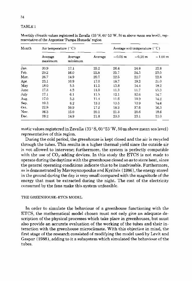
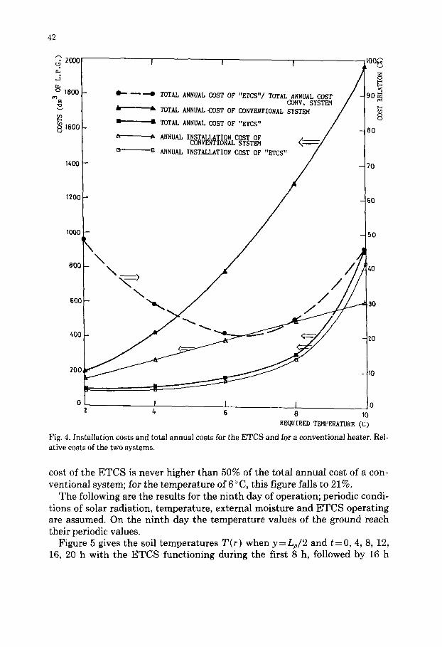
Figure 4 shows the installation costs and the total running costs per annum for both systems in function of the minimum temperature. The cost relation (in percentages) is also given. The cost relation reveals that the total annual

42

L; 2OOO J o 1800

~SO0 L)

1400

1200

I I I

~ "--'0 TOTAL ANNUAL COST OF "ETCS"/ TOTAL ANNUAL COST CONV.

*- :- TOTAL ANNUAL COST OF CONVENTIONAL SYSTEM SYSTEM

TOTAL ANNUAL COST OF "ETCS" / a L ANNUAL INSTALLATION COST OF / /

CONVENTIONAL SYSTF24

ANNUAL INSTALLATION COST OF "ETCS"

E4

80

1000 ~'~- /

400

r"

o ~ I f I 4 6 8 tO

REQUIRED TEMPERATURE (C)

Fig. 4. Instal la t ion costs and total annual costs for the ETCS and for a convent ional heater. Rel- ative costs of the two systems.

- 7 0

50

- 50

~40

30

20

10

cost of the ETCS is never higher than 50% of the total annual cost of a con- ventional system; for the temperature of 6°C, this figure falls to 21%.

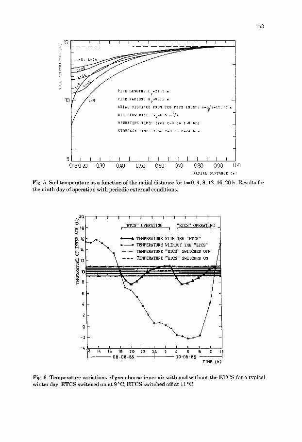
The following are the results for the ninth day of operation; periodic condi- tions of solar radiation, temperature, external moisture and ETCS operating are assumed. On the ninth day the temperature values of the ground reach their periodic values.

Figure 5 gives the soil temperatures T(r) when y=Lp/2 and t=O, 4, 8, 12, 16, 20 h with the ETCS functioning during the first 8 h, followed by 16 h

43

~15

t=O, t=24

o

O P E R A T I ~ TIME: f r o m t=O t o t=8 hrs

0.]5 0.20 030 0.40 0.50 060 0.70 OBO 090 100 RADIAL DISTANCE (m)

Fig. 5. Soil temperature as a function of the radial distance for t=O, 4, 8, 12, 16, 20 h. Results for the n i n t h day of operat ion wi th periodic external conditions.

2 O c.) v

2

0

-2

-412

I [ I I I I I I I I i

"ETCS" OPERATING "ETCS" OPERATING | m s !

• TEMPERATURE WITH THE "ETCS"

o TEPIPERATURE WITHOUT THE "ETCS"

TEMPERATURE "ETCS" SWITCHED OFF

TEMPERATURE "ETCS" SWITCHED ON

-

! i I I I I I I I I I 14 t6 18 20 22 2~4 2 4 G 5 10

os-os-ss I 09-05-85 i

TIHE (h)

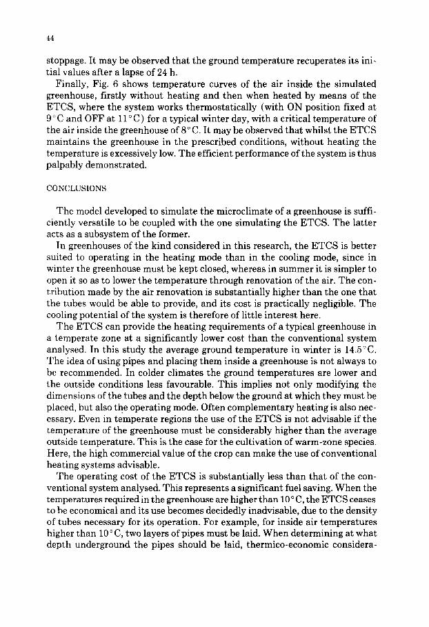
Fig. 6. Tempera ture var ia t ions of greenhouse inner air wi th and wi thout the ETCS for a typical winter day. E T C S switched on at 9 ° C; ETCS switched off a t 11 ° C.

44

stoppage. It may be observed that the ground temperature recuperates its ini- tial values after a lapse of 24 h.

Finally, Fig. 6 shows temperature curves of the air inside the simulated greenhouse, firstly without heating and then when heated by means of the ETCS, where the system works thermostatically (with ON position fixed at 9 °C and OFF at 11 °C ) for a typical winter day, with a critical temperature of the air inside the greenhouse of 8 ° C. It may be observed that whilst the ETCS maintains the greenhouse in the prescribed conditions, without heating the temperature is excessively low. The efficient performance of the system is thus palpably demonstrated.

CONCLUSIONS

The model developed to simulate the microclimate of a greenhouse is suffi- ciently versatile to be coupled with the one simulating the ETCS. The latter acts as a subsystem of the former.

In greenhouses of the kind considered in this research, the ETCS is better suited to operating in the heating mode than in the cooling mode, since in winter the greenhouse must be kept closed, whereas in summer it is simpler to open it so as to lower the temperature through renovation of the air. The con- tribution made by the air renovation is substantially higher than the one that the tubes would be able to provide, and its cost is practically negligible. The cooling potential of the system is therefore of little interest here.

The ETCS can provide the heating requirements of a typical greenhouse in a temperate zone at a significantly lower cost than the conventional system analysed. In this study the average ground temperature in winter is 14.5°C. The idea of using pipes and placing them inside a greenhouse is not always to be recommended. In colder climates the ground temperatures are lower and the outside conditions less favourable. This implies not only modifying the dimensions of the tubes and the depth below the ground at which they must be placed, but also the operating mode. Often complementary heating is also nec- essary. Even in temperate regions the use of the ETCS is not advisable if the temperature of the greenhouse must be considerably higher than the average outside temperature. This is the case for the cultivation of warm-zone species. Here, the high commercial value of the crop can make the use of conventional heating systems advisable.

The operating cost of the ETCS is substantially less than that of the con- ventional system analysed. This represents a significant fuel saving. When the temperatures required in the greenhouse are higher than 10 o C, the ETCS ceases to be economical and its use becomes decidedly inadvisable, due to the density of tubes necessary for its operation. For example, for inside air temperatures higher than 10 ° C, two layers of pipes must be laid. When determining at what depth underground the pipes should be laid, thermico-economic considera-

45

tions should not be the only decisive factors. Provision should also be made for the root temperatures not decreasing perceptibly, since this could have a neg- ative effect upon the crop development.

Maintenance of the system is simple: it is limited to maintaining the fans and thermostat , plus occasional cleaning of the pipes to remove any dust or live organisms that may have accumulated inside the tubes. The cleaning pro- cess is facilitated by the sloping of the tubes.

The use of the ETCS appears to be well justified in greenhouses, whereas enclosures designed for human residences or livestock housings generally re- quire higher temperatures. The major advantages of this system are that it protects the crops against frost and enables the vital functions of certain crops to continue.

LIST OF SYMBOLS

Ab Ac Af Av Cp C DT De D0,vap hi h. h~ ht hv ks Lai Ldc Ldp Lds Lec Loc Lp Luc Lup Lus rh~ n Qc

floor area of greenhouse (m 2) cover surface area (m 2) frontal surface area of greenhouse (m 2) floor area covered by vegetation (m 2) specific heat of air (J kg -1 K -1) volumetric thermal capacity of soil (J m -3 K - 1 ) thermal moisture diffusivity (m 2 s - 1 K - ~ ) isothermal moisture diffusivity (m 2 s-1) isothermal diffusivity of moisture in vapour form (m 2 s - ~ ) heat transfer coefficient of floor to internal air (W m -2 K -1) heat t ransfer coefficient of plants to internal air (W m -2 K - ~ ) heat t ransfer coefficient of cover to internal air (W m -2 K -~) heat transfer coefficient of tube to air (W m -2 K -1) heat transfer coefficient by ventilation (W m -2 K - ~ ) thermal conductivity of soil (W m-1 K - ' ) leaf area index (foliage area per unit floor area) downward thermal radiation from cover (W m -2) downward thermal radiation to plants (W m -2) downward thermal radiation to floor (W m-2) upward thermal radiation from cover (W m -2) downward thermal radiation to cover (W m -2) pipes length (m) upward thermal radiation to cover (W m-2) upward thermal radiation from plants (W m -2) upward thermal radiation from floor (W m - 2 ) mass flow rate of the air through pipe (kg s -~) number of tubes energy by convection from heaters (W)

46

r RL Rp Sd Se So Ssd Ssu Su S, t T Ta Tap We Tic Toe

T, 7s U va VR

Y 2

P Pl 0 (2)

0 9 e

O)sc O)sp

O)ss

radial distance from the tube axis (m) arbitrarily large radial distance (m) pipe radius (m) solar radiation going down from cover (W m -z) solar radiation going up external house (W m -2) incident solar radiation flux (W m -z) solar radiation to floor (W m -2) solar radiation going up from floor (W m -2) solar radiation to cover (W m -e) spraying rate (kg min -1 ) time (s) ground temperature (K) internal air temperature (K) air temperature along the pipe (K) external temperature (K) internal cover temperature (K) outside cover temperature (K) temperature at the tubes outlet (K) plant leaves temperature (K) greenhouse soil temperature (K) use factor (on/off) velocity of air (m s - 1 ) ventilation rate (m 3 s - 1 )

axial distance from the tube inlet (m) latent heat of vaporization of water (J kg- 1 ) air density (kg m -a) density of moisture (kg m -:~) volumetric moisture content (m 3 of mois ture /m 3 of moist soil) specific humidity of internal air specific humidity of external air saturation specific humidity at temperature Tie saturation specific humidity at temperature Tp saturation specific humidity at temperature T~

REFERENCES

Ewen, L.S, Walker, J.N. and Buxton, J.W., 1980. Environment in a greenhouse thermally buffered with ground-conditioned air. Trans. ASAE, 23: 985-989.

IMSL, 1983. TWODEPEP User's Manual. International Mathematical and Statistical Libraries, Houston, U.S.A.

Kozai, T., 1985. Thermal performance of a solar greenhouse with an underground heat storage system. Proc. Int. Syrup. on Thermal Application of Solar Energy, Hakone, Japan, pp. 503- 508.

Kurata, K. and Takakura, T., 1985. Simulation of climate within a solar greenhouse equipped with

47

underground heat storage units. Proc. Int. Symp. on Thermal Application of Solar Energy, Hakone, Japan, pp. 521-526.

Levit, H.J. and Gaspar, R., 1988. Energy budget for greenhouses in humid-temperate climate. Agric. For. Meteorol., 42: 241-254.

Mavroyanopoulus, G.N. and Kyritsis, S., 1986. The performance of greenhouse heated by an earth- air heat exchanger. Agric. For. Meteorol., 36: 263-268.

Peterson, W.O., Walker, J.N., Duncan, G.A. and Anastasi, D.T., 1975. Composition of coal mine air in relationship to greenhouse environment control. Trans. ASAE, 18: 140-144.

Puri, V.M., 1986. Feasibility and performance curves for intermittent earth tube heat exchangers. Trans. ASAE, 29: 526-532.

Puri, V.M., 1987. Earth tube heat exchanger performance correlation using boundary element method. Trans. ASAE, 30: 514-520.

Walker, J.N., Peterson, W.O., Duncan, G.A. and Anastasi, D.T., 1977. Temperature and humidity in a greenhouse ventilated with coal mine air. Trans. ASAE, 19: 311-317.