Simulation of Hemiplegic Subjects’ Locomotion

Nicolas Fusco, Guillaume Nicolas, Franck Multon, and Armel Cretual

Laboratoire de Physiologie et de Biomecanique de l’Exercice MusculaireRennes 2 University, Av. Charles Tillon CS 24414, 35044 Rennes, France

{nicolas.fusco, guillaume.nicolas, franck.multon, armel.cretual}@uhb.fr

Abstract. This paper aims at describing a new method to simulatethe locomotion of hemiplegic subjects. To this end, we propose to useinverse kinematics in order to make the feet follow a trajectory with re-spect to the root frame linked to the pelvis. The 11 degrees of freedomare then retrieved by inversing the kinematic function while taking otherconstraints into account. These constraints, termed secondary tasks im-pose that the solution ensures joints limits and energy minimisation. Inaddition to those general constraints, the main originality of this workis to take spasticity into account. This new constraint is obtained ac-cording to the specificity of the subject’s pathology. The results showthat angular trajectories for the pelvis, the hips and the knees for thesimulated and the real motion are very similar. This preliminary workis promising and could be used to simulate the effects of reeducation ormedical treatments on patients’ gait.

Keywords: inverse kinematics, locomotion, hemiplegia, spasticity.

1 Introduction

Using computer simulation and animation in biomechanics is a new approach toperforming motion analysis. Nevertheless, animation based only on kinematicscould generate unrealistic movements. Hence, to simulate human locomotion, alarge set of solutions is proposed in the literature [1]. Among these techniques,inverse kinematics is widely used to ensure foot-contact with the ground withoutsliding [2] or to adapt an existing movement to a different skeleton [3].

Several past works [4] have proposed an explicit method to solve inverse kine-matics problems for limbs composed of only a few segments. These methodsare efficient for isolated upper and lower limbs but seem difficult to apply tothe whole body. To deal with more complex structures, the problem is gener-ally solved using a linear approximation of the direct kinematics equation [5].In some cases, several constraints can be applied, for example, controlling sev-eral extremities or constraining centre of mass movements. This problem can besolved by weighting each constraint [6]. [7] proposed a task-priority formulationto take all of these constraints into account.

Whatever the technique is, because of the redundancy, there generally existsan infinity of possible solutions. A secondary task is then proposed to selecta specific solution. The main problem is to determine the constraints that will

S. Gibet, N. Courty, and J.-F. Kamp (Eds.): GW 2005, LNAI 3881, pp. 236–247, 2006.c© Springer-Verlag Berlin Heidelberg 2006

Simulation of Hemiplegic Subjects’ Locomotion 237

help to compute a human-like movement. To this end, several methods have beenproposed. [8] offered to select the solutions that are close to captured trajecto-ries for arm movements. [9] added a weight matrix in the resolution process. Theweights were identified by optimisation until the calculated movement resembleda captured one. All these approaches are based on real movements and cannotbe used if no knowledge on the resulting movement is available (such as for simu-lating new behaviors). A more general approach is to control also the position ofthe centre of mass [10]. These methods are well adapted to quasi-static motions,but are not suitable for movements involving dynamics such as locomotion.

Simulating a human-like motion is a complex problem because a large numberof parameters has to be considered, including energy, comfort, equilibrium, jointlimits, muscle activation, etc. To simulate such specific locomotion of subjectswith hemiplegia, the nature of the pathology also has to be considered. In thispaper, we focus on hemiplegic subjects with spasticity. The spasticity engen-ders an increase in the stretching reflex linked to speed of muscle contraction.As a consequence, the locomotion of such subjects is generally dissymmetricwith lower speeds than those of healthy subjects. [11] demonstrated that thereis no correlation between dissymmetry and walking speed but that individualbehaviors occurred. This result indicates that no general method can be directlyapplied to a patient. [12, 13] reported a lower hip flexion during the balance phaseand a lower hip extension after foot-strike. They also pointed-out an exagger-ated knee flexion at foot-strike and a lower knee flexion at the balance phase.The latter is explained by a deficiency of the motor controller and spasticityof the rectus femoris and the gastrocnemius. [14] demonstrated that cocontrac-tions disorders influenced the metabolic energetic cost of walking in patients withcerebral palsy. Moreover, several authors demonstrated that hemiplegic patientsgenerally spend more energy than healthy subjects do for walking at the samespeed [15, 16]. However, this difference tends to decrease when walking speedincreases [17]. In fact, the more the self-selected velocity of hemiplegic subjectsis near that of healthy subjects, the more the difference tends to decrease. Thismeans that self-selected speed is a reliable index of pathology level. Individ-ual behaviors were again pointed-out. Of course, computer simulation makes itimpossible to measure directly energy expenditure. However, [18] demonstratedthat mechanical power estimates correctly the O2 cost of walking in subjectswith hemiplegia. As a consequence, energy requirements of a simulated walkcould be approximated by the computation of the corresponding internal work.

In this paper, we propose a new approach to simulate locomotion of hemiplegicsubjects with cerebral palsy. To do so, we propose to model spasticity through itseffects on the stretching reflex that decrease joint limits and angular velocity. Wefocus on the rectus femoris and gastrocnemius that directly act on knee flexionand extension. The method described in sections 2 is applied to a skeleton thatwas fitted to anatomical landmarks taken on a real hemiplegic subject. Thistechnique is based on inverse kinematics and secondary tasks are used to takepathology into account. In section 3, the simulated angular trajectories are thencompared to those of this subject to evaluate the model’s efficiency.

238 N. Fusco et al.

2 Modelisation

2.1 Inverse Kinematics to Model Human Locomotion

Given a set of anatomical landmarks measured on a real subject, we are ableto construct the kinematic function that links the angular representation of theposture to the position of lower-body extremities. In this study, we focus onthe lower-body including the pelvis, femurs and tibias. The root frame of thekinematic chain has its origin at the middle of the pelvis. Its orientation isfixed meaning it has the same orientation as the pseudo-Galilean frame linkedto the laboratory. The pelvis can rotate along its main axes, i.e. it has 3 degreesof freedom (DOF). Each hip is associated to 3 new DOF which simulate theflexion/extension, adduction/abduction and medial and lateral rotation of thistypical ball and socket joint. Each knee is considered as a hinge joint with 1DOF corresponding to the flexion/extension. The system is thus composed of 11DOF (Fig. 1). The root frame is in fact that of the pelvis at the initial posturewith every angle set to zero.

Root frame

3 rotations

��Pelvis frame

3 rotations

������

�������3 rotations�����

�������

Left femur frame

1 rotation

��

Right femur frame

1 rotation

��Left tibia frame Right tibia frame

Fig. 1. Structure of the 11-DOF skeleton

Hence, the position of each ankle with respect to F is:

X = f (θ) (1)

where X = (xl, yl, zl, xr, yr, zr) is the position of the effectors with respect to theCartesian position of the left and the right ankle, θ stands for the 11-dimensionalvector of angles applied to the DOF. The set of all θ is called configuration space.From equation 1, we numerically compute the Jacobian of the system:

∆X = J (θ)∆θ (2)

Given, the trajectories of the ankles in the root frame, referred to as poulainein the remainder of the paper, the primary task is ensured by inversing equation2:

∆θ = J+ (θ)∆X (3)

Simulation of Hemiplegic Subjects’ Locomotion 239

where J+ is the pseudo-inverse of J. As 6 constraints are applied to this 11-DOFsystem, that leads to a 5-dimensional kernel space of J , termed Ker. This kernelis the image of the configuration space by the matrix (I − J+J), I being theunity matrix. Nevertheless, nothing ensures that the solution proposed with thisequation verifies constraints such as joint limits or energy expenditure minimisa-tion. For this, a secondary task z is generally proposed to take those constraintsinto account [5]:

∆θ = J+ (θ) ∆X + α(I − J+J

)∇z (4)

where α is a weight associated with the secondary task and z stands for a costfunction to minimise. Generally, this secondary task is solved iteratively withthe steepest descent method. On one hand, if several constraints are proposedconcurrently, the system tries to solve a least square problem. A compromise ofall the conditions is consequently found with this method. On the other hand,some of the constraints (such as preserving joint limits) require strict verificationwhile others (such as energy expenditure) only need to be minimised.

2.2 Specifying Pathology Using the Secondary Task

When the primary task is solved we obtain an initial value ∆θm :

∆θm = J+∆X (5)

This solution has a minimal norm but nothing ensures that it respects jointlimits and produces realistic trajectories. If ∆θm is a solution of equation 3 andφ an element of Ker, then ∆θm + φ is also a solution of equation 3. The goal ofthe secondary tasks is to find the optimal φ that minimises a set of functions.Let us call θt the current value of θ. To model the specific gait of hemiplegicsubjects, we chose the functions below:

– T1: To account for joint limits, we defined a continuous and derivable costfunction that rapidly increases beyond the joint limits. In this paper, wepropose an exponential function:

f1 (θt, ∆θm, δ) =∑11

i=1

(eζ(αi−bupi) + eζ(blowi−αi)

)

with α = (θt + ∆θm + (I − J+J) δ)(6)

where bupi and blowi are respectively the upper and the lower joint limits forthe ith DOF. ζ is a constant coefficient that ensures a rapid increase whenthe angle is beyond the joint limits and a rapid decrease when it is withinthose limits (Fig. 2). δ is any element of the configuration space.

For subjects with cerebral palsy causing knee flexion/extension disorders,the joint limits are customised. Hence, the maximum and minimum kneeangle were obtained specifically for this subject. A new function taking thespasticity into account by also constraining the knee angular velocity witha maximum value has been defined. This value was obtained by computing

240 N. Fusco et al.

−0.5 −0.4 −0.3 −0.2 −0.1 0 0.1 0.2 0.3 0.4 0.50

0.5

1

1.5

2

2.5

3

3.5x 10

10

Angle (rad)

Cos

t fun

ctio

n f1

Fig. 2. Cost function f1 depending on an angle giving a maximum and a minimumjoint limit

the maximum angular velocity of the affected knee while walking at themaximum speed. This angular velocity was multiplied by an empirical factor1.2 to take a 20 % offset into account. The resulting angular velocity canvary between 0 and max by adding a new function f1bis

.

f1bis(θt, ∆θm, δ) = eζ(αknee−vup) + eζ(vlow−αknee)

with αknee = (θt + ∆θm + (I − J+J) δ)knee

(7)

where αknee is the knee angle of the affected side and αknee its angular ve-locity, vup and vlow are respectively the upper and the lower knee angularvelocity limits. ζ is a constant coefficient that ensures a rapid increase whenthe velocity is beyond the knee angular velocity limits and a rapid decreasewhen it is within those limits.

– T2: minimising the rotational kinetic energy of each body segment:

f2 (θt, ∆θm, δ) =5∑

b=1

[12RbIbR

Tb

(wb

((I − J+J)δ, ∆θm

))2

]

(8)

where b stands for the body segment index, Ib is the inertia of segment b.wb is a function that computes the angular velocity vector of segment b de-pending on ∆θm and the optimized parameter δ. Rb is the transform matrixbetween the body segment frame and the root frame, computed from θt.

Simulation of Hemiplegic Subjects’ Locomotion 241

– T3: searching for a solution close to the rest posture:

f3 (θt, ∆θm, δ) =∥∥θt + ∆θm +

(I − J+J

)δ − θr

∥∥2 (9)

where θr is the angle at rest posture provided by motion capture on statictrials.

We propose to use the Multidirectional Search (MDS) method [19] to solvethis secondary tasks problem. It enables one to minimise cost functions wetherthere are derivable or not and is less sensible to local minimum than the steepestdescent method.

According to an initial value which is the posture at the previous time step,MDS evaluates among a set of neighbours the cost function fi. The neighboursare selected by using a simplex ∆ that is linked to all the main axes of the searchspace:

∆j = {∀i, δj + β · unit (i)} (10)

where δj is the current solution at step j, β stands for the size of the simplexand unit(i) is a vector composed with zeros excepted for the ith element (equalto 1). ∆j is a set of candidates that can be evaluated thanks to the cost function.In order to cover a wider space of research, two operators are used: a contraction(× 0.5 in our examples) and an expansion operator (× 2 in our examples). Thosetwo operators modify the simplex size by scaling it by real factors respectivelylower and greater than 1. Among all the resulting candidates, the system selectsthe one that minimises the cost function. This candidate becomes the new cur-rent solution δj+1. The process is repeated until a stable solution δ is obtainedor the cost function goes under a given threshold ε set to 10−4 in our example.

The optimal solution of the inverse kinematics problem is given at nextstep by:

θt+∆t = θt + ∆θm +(I − J+J

)δ (11)

3 Experimental Validation

3.1 Experimental Set Up and Procedure

A volunteer with hemiplegia participated in this experiment after giving in-formed consent. The subject age, height and mass were 25 years, 1.8 m andmass 83 Kg respectively. This patient with cerebral palsy suffered from spastic-ity of the right rectus femoris and right gastrocnemius so that his locomotion wasclearly affected. Three-dimensional kinematics of the subjects hemiplegic lowerextremity were documented with the Vicon370 motion analysis system (prod-uct of Oxford Metrics, Oxford, UK). Seven infrared, 60 Hz cameras recordedthe location of thirty reflective markers placed over standardized anatomicallandmarks overlying the bony landmarks (Fig. 3). The subject’s motion datawas captured during gait test on a treadmill for walking speeds increasing from0.5 to 1.1 m.s−1. Finally, the poulaines which are the effectors’ position for the

242 N. Fusco et al.

Fig. 3. Anatomical landmarks used for motion capture

primary task, were obtained on the subject walking at 0.5 m.s−1. Given thesepoulaines, the problem is to calculate realistic angular trajectories.

In order to evaluate the resulting simulation, we proposed to calculate theRoot Mean Square (RMS) which evaluates the difference between the simulatedand the captured trajectories:

Ci =

√√√√ 1

T

T∑

t=0

(θi (t) − θi (t)

)2(12)

where t stands for the time and T for the total duration, i for the DOF and θi

for the captured trajectory. In this equation, θi is shifted to θi mean value.

3.2 Results

First, Fig. 4 shows that the primary task is absolutely ensured. In fact, the RMSerrors between the captured poulaines and those simulated are less than 1 mm.

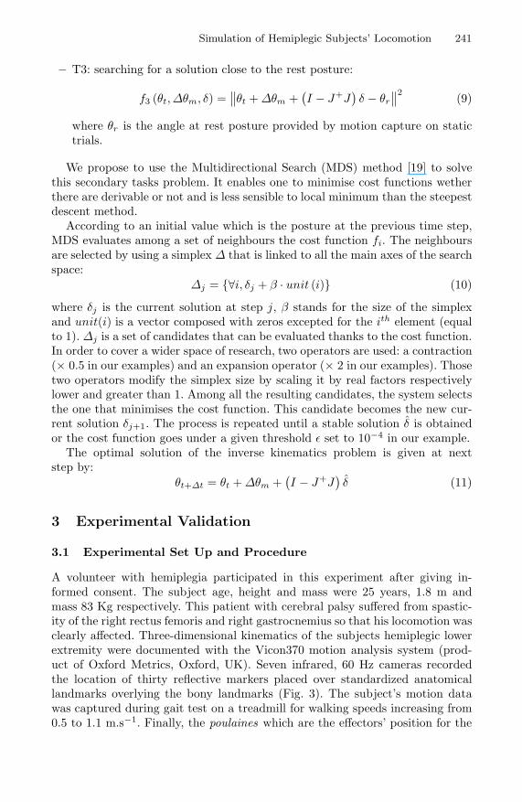
Second, in Fig. 5, one can see simulated (continuous line) and experimen-tal data (dashed line) angular trajectories for the hips and the knees. All thesimulated trajectories have a similar shape compared to real ones.

Regarding the subject’s pathological specificity, the simulated angular trajec-tories of the affected side show a lower hip flexion during the balance phase anda lower hip extension after foot-strike. However, the differences (around 0.1 rad)

Simulation of Hemiplegic Subjects’ Locomotion 243

−0.05 0 0.05 0.1 0.15−0.95

−0.9

−0.85

−0.8

−0.75

−0.7

Left poulaines captured compared with those simulated on X et Z axis

Distance (m)

Dis

tanc

e (m

)

0 0.1 0.2 0.3 0.4 0.5−0.95

−0.9

−0.85

−0.8

−0.75

−0.7

Left poulaines captured compared with those simulated on Y et Z axis

Distance (m)

Dis

tanc

e (m

)

−0.25 −0.24 −0.23 −0.22 −0.21 −0.2−0.92

−0.9

−0.88

−0.86

−0.84

Right poulaines captured compared with those simulated on X et Z axis

Distance (m)

Dis

tanc

e (m

)

−0.1 0 0.1 0.2 0.3 0.4−0.92

−0.9

−0.88

−0.86

−0.84

Right poulaines captured compared with those simulated on Y et Z axis

Distance (m)

Dis

tanc

e (m

)

left poulaine capturedleft poulaine simulated

right poulaine capturedright poulaine simulated

left poulaine capturedleft poulaine simulated

right poulaine capturedright poulaine simulated

Fig. 4. Simulated and captured poulaines for the healthy and the affected leg, in thefrontal plane on the left and in the sagittal plane on the right

with the healthy leg are small. Futhermore, as reported in previous works [20]the flexion of the healthy knee resembles a shape classically encountered withhealthy subjects. However, the flexion of the affected knee is far from a classicalshape encountered with healthy subjects. We observe an exaggerated knee flex-ion at foot-strike and a lower knee flexion at the balance phase on the affectedside compared to the healthy one. The maximal flexion of the healthy side is1.15 rad against 0.74 rad for the affected side.

Third, for the differents joints, as those reported in Table 1, the results showedare very close to the real trajectory. Indeed, the RMS error value between thesimulated and the real angular trajectory is lower or equal to 0.11 rad.

In the same way, we compare the RMS error between the simulated Cartesianposition of each joint with those of the real movement. Again, Table 2 reportederror equal or less than 10 mm. These results indicate that Cartesian positionsare ensured by the simulation.

The results exhibit very similar Cartesian position while the angular trajecto-riese simulated are very close to real ones for all the articulations. Nevertheless,some differences occur. This seems to be mainly due to two reasons. First, theapplication of the captured, and thus, noisy poulaine to the virtual patient. Thispoulaine is obtained thanks to markers that slide over the skeleton. As proofof this sliding, for some points, we obtain an instantaneous distance between

244 N. Fusco et al.

0 20 40 60 80 100

1.6

1.8

2

2.2Left Hip

Time (% cycle)

Ang

le (

rad)

0 20 40 60 80 1001.5

1.6

1.7

1.8

1.9

2Right Hip

Time (% cyle)

Ang

le (

rad)

0 20 40 60 80 1000.4

0.6

0.8

1

1.2

1.4Left Knee

Time (% cyle)

Ang

le (

rad)

0 20 40 60 80 1000.4

0.5

0.6

0.7

0.8Right Knee

Time (% cyle)

Ang

le (

rad)

(a)

(c)

(b)

(d)

Fig. 5. Simulated (continuous line) vs. captured (dashed line) angular trajectories forthe hips (a and b) and the knees (c and d)

Table 1. RMS error between the simulated and the real angular trajectories

Joints’ angles RMS (rad)Pelvis inclination 0.03Pelvis obliquity 0.10Pelvis int/ext rotation < 0.01Left Hip fle/ext 0.01Left Hip abd/add < 0.01Left Hip int/ext rotation 0.03Right Hip fle/ext 0.01Right Hip abd/add < 0.01Right Hip int/ext rotation 0.10Left Knee fle/ext 0.11Right Knee fle/ext < 0.01

markers greater than dimensions calculated in the static trial. For example, theminimum knee flexion is equal to 0.45 rad for the healthy knee in the real angulartrajectories. This is a very high value since this time corresponds to a foot-strikewhere the knee is supposed to be quite extended. This problem could be solved

Simulation of Hemiplegic Subjects’ Locomotion 245

Table 2. RMS error between the simulated and the real postion trajectories

Joints’ position Axis RMS (mm)x 4

Left trochanter y 9z 5x 3

Right trochanter y 5z < 1x 1

Left Knee y 10z 4x 1

Right Knee y 1z < 1

by retrieving actual joint centres instead of directly using external markers. Sec-ond, we may implicate the choice of the secondary task. In fact, the secondarytask does not take into account all the parameters of the subject’s gait and hispathology.

4 Discussion

We described a preliminary work to simulate the gait of hemiplegic subjectswith cerebral palsy. The pathology of a subject was modeled through constraintequations. Those equations are obtained according to the subject’s pathologyspecificity. The subject had a spasticity of the rectus femoris and of the gastroc-nemius that engendered knee flexion disorders. We consequently proposed tomodel its pathology by adding a function limiting his minimum and maximumknee flexion and knee flexion velocity.

This methodological work obviously requires validation on a wider set of sub-jects. Moreover, the poulaine that is applied as an entry of our model also con-tains information linked to the subject pathology. To validate our model, it couldbe interesting to use other poulaines : ranging from other subjects with cerebralpalsy to healthy one.

The possible applications of such a model are linked to reeducation.First, it could allow us to carry-out fundamental research on the links be-

tween all disorders encountered with hemiplegic subjects. Hence, in the liter-ature, the main problem is to define cause-to-effect links between observablephenomena [18]. Nevertheless, as locomotion is the consequence of a large setof coupled parameters, it is impossible to isolate the effect of one of them onanother. With simulation, it is possible to change only one parameter and verifyits consequences. For example, are the knee flexion disorders greater than stepduration dissymmetry for energy expenditure?

Second, for reeducation, this kind of model could be used to evaluate possibleconsequences of several methods on energy expenditure. In the literature, it

246 N. Fusco et al.

is demonstrated that knee flexion disorders causes a raising of the trunk andthe pelvis in the frontal plane during the balance phase of the affected leg. Toovercome this problem, it has been proposed to use controlateral shoe-lifts thatallow the subject to balance the leg without touching the ground and rotatingthe pelvis. If the goal is to decrease energy expenditure while walking in everydaylife, is this strategy more interesting than retrieving a larger knee flexion?

For both applications, the poulaine could be captured on the patients so thatthe main limitation of our method is lowered. Indeed, the goal is to have acomputer model walk as the real model while only changing a minimum setof parameters (increasing joint limits, scaling the poulaine to increase the steplength, time-scaling the poulaine to obtain symmetrical cyles for examples).

Acknowledgements

This work was partially funded by the Conseil Regional de Bretagne (BritannyRegional Council). We also thank H. Gain and Dr. P. Le Cavorzin for their helpin the selection of the patient.

References

1. Multon, F., France, L., Cani-Gascuel, M., Debunne, G.: Computer animation ofhuman walking: a survey. Journal of Visualization and Computer Animation 10(1999) 39–54

2. Boulic, R., Thalmann, D.: Combined direct and inverse kinematic control forarticulated figures motion editing. Computer Graphics Forum 11 (1992) 189–202

3. Monzani, J., Baerlocher, P., Boulic, R., Thalmann, D.: Using an intermediateskeleton and inverse kinematic for motion retargeting. In: Eurographics, Interlaken(2000)

4. Tolani, D., Badler, N.: Real-time inverse kinematics of the human arm. Presence,Teleoperators, and Virtual Environments 5 (1996) 393–401

5. Baerlocher, P.: Inverse kinematics techniques for the interactive posture control ofarticulated figures. PhD thesis, EPFL, Switzerland (2001)

6. Philips, C., Zaho, J., Badler, N.: Interactive real-time articulated figure manipula-tion using multiple kinematic constraints. Computer Graphics 24 (1990) 245–250

7. Baerlocher, P., Boulic, R.: Task-priority formulations for the kinematic control ofhighly redundant structures. In: IEEE IROS’98. (1998) 323–329

8. Wang, X., Verriest, J.: A geometric algorithm to predict the arm reach posture forcomputer-aided ergonomic evaluation. The Journal of Visualization and ComputerAnimation 9 (1998) 33–47

9. Zhang, X., Kuo, A., Chaffin, D.: Optimization-based differential kinematic mod-eling exhibits a velocity-control : strategy for dynamic posture determination inseated reaching movements. Journal of Biomechanics 31 (1998) 1035–1042

10. Boulic, R., Mas, R., Thalmann, D.: Complex character positioning based on acompatible flow model of multple supports. IEEE Transactions on Visualizationand Computer Graphics 3 (1997) 241–261

11. Feys, H., De Weerdt, W., Nieuwboer, A., Nuyens, G., Hanston, L.: Analysis of tem-poral gait characteristics and speed walking in stroke patients and control group.Musculoskeletal Management 1 (1995) 73–85

Simulation of Hemiplegic Subjects’ Locomotion 247

12. Olney, S., Griffin, M., Monga, T., Mc Bride, I.: Work and power in gait of strokepatients. Archives physical medicine and rehabilitation 72 (1991) 309–314

13. Olney, S., Richards, C.: Hemiparetic gait following stroke. part i: Characteristics.gait and posture 4 (1996) 136–148

14. Viswanath, B., Dowling, J., Frost, G., Bar-Or, O.: Role of cocontraction in the o2cost of walking in children with cerebral palsy. Medicine and Science in Sports andExercise (1996) 1498–1504

15. Olney, S., Monga, T., Costigan, P.: Mechanical energy of walking of stroke patients.Archives physical medicine and rehabilitation 67 (1986) 92–98

16. Waters, R., Mulroy, S.: The energy expenditure of normal and pathologic gait.Gait and Posture 9 (1999) 207–231

17. Zamparo, P., Francescato, M., De Luca, G., Lovati, L., Di Prampero, P.: Theenergy cost of level walking in patients with hemiplegia. Scandinavia Journal ofMedicine and Science in Sports 5 (1995) 348–352

18. Viswanath, B., Dowling, J., Frost, G., Bar-Or, O.: Role of mechanical powerestimates in the o2 cost of walking in children with cerebral palsy. Medecineand Science in Sports and Exercise (1999) 1703–1708

19. Torczon, V.: Multi-directional Search: A Direct Search Algorithm for ParallelMachines. Ph.d. thesis, Rice University, Houston,Texas, USA (1989)

20. Burdett, R., Skrinar, G., Simon, S.: Comparison of mechanical work and metabolicenergy consumption during noram gait. Journal of Orthopaedic Research 1 (1983)63–72