SIMULATION OF PRESSURE VARIATIONS WITHIN KIMILILI WATER SUPPLY SYSTEM USING EPANET

International Journal of Civil Engineering and Technology (IJCIET), ISSN 0976 – 6308 (Print),

ISSN 0976 – 6316(Online), Volume 6, Issue 4, April (2015), pp. 28-38 © IAEME

28

SIMULATION OF PRESSURE VARIATIONS WITHIN

KIMILILI WATER SUPPLY SYSTEM USING EPANET

CHRISTOPHER BWIRE1,

RICHARD ONCHIRI2, NJENGA MBURU

3

1Post Graduate Student, Masinde Muliro University of Science and Technology, Department of Civil

and Structural Engineering, P.O.Box 190-50100 Kakamega

2Lecturer, Masinde Muliro University of Science and Technology, Department of Civil and

Structural Engineering, P.O.Box 190-50100 Kakamega, Kenya

3Lecturer, Dedan Kimathi University of Technology, Department of Civil and Structural

Engineering, P.O.Box 657-10100 Nyeri, Kenya

ABSTRACT

Water Supply system is a system of engineered hydrologic and hydraulic components which

provide water supply for domestic use, industrial purposes, fire fighting and so on. The system

comprises of intake structures, treatment units, storage tanks and distribution systems. A well

designed water supply system is meant to operate optimally such that consumers have access to

portable water of sufficient pressure and quality at all times. However during operations of water

supply systems, cases of pressure drops, Leakages and contamination occur and the main challenge

is the lack of a simple tool to accurately predict zones of low pressures and areas where quality is

compromised. This study will investigate the operations of Kimilili Water Supply system in

Bungoma County in terms of pressure Variations from the Treatment Works to the consumer points.

The main objective of the study is to simulate pressure variations in the distribution system using

EPANET software and Compare with measured data in the field. The EPANET programme analyses

the pressure at each node, track the flow of water in each pipe and height of the Water in each tank

during simulation period. After simulation of the whole Water Supply system, results were presented

in various forms and compared with the field measured data using pressure loggers. Simulated water

pressure did not vary significantly with the actual values indicating that the pipes still had their

hydraulic capacities even though some sections of the network need augmentation.

Keywords: Hydraulic Simulation, Water Pressure, Pressure Variation, Nodes, Pressure Logger

INTERNATIONAL JOURNAL OF CIVIL ENGINEERING AND

TECHNOLOGY (IJCIET)

ISSN 0976 – 6308 (Print)

ISSN 0976 – 6316(Online)

Volume 6, Issue 4, April (2015), pp. 28-38

© IAEME: www.iaeme.com/Ijciet.asp

Journal Impact Factor (2015): 9.1215 (Calculated by GISI)

www.jifactor.com

IJCIET

©IAEME



29

1. INTRODUCTION

A water supply system consists of source, treatment, distribution and storage facilities whose

main function is for domestic water supply, industrial as well as fire fighting purposes. A water

distribution network is composed of a number of links connected together to form loops or branches.

The links are composed of pumps, fittings and valves. Links have constant flow with no branches.

Water supply systems have also nodes which are basically end points of the pipe where two or more

links are joined. Water distribution network analysis follows the continuity equation where the

algebraic sum of flow rates in the pipes meeting at a node together with any external flows is zero.

The water supplied by a municipal water supply system meets the three levels of usage as follows

a) The average daily demand which reflects the amount of water used per day and does not

consider occupancy differences such as commerce and industry

b) The maximum daily consumption which reflects the day within a year long period on which

the consumption was highest. This figure is approximately 150% of the average daily demand.

c) The instantaneous flow demand which represents peak flows i.e when consumption is highest

between 7 a.m -9a.m and between 5p.m and 7p.m. During the peak period the flows can reach

as high as 225% of the average daily demand [8].

It is therefore imperative that municipal water supplies are able to deliver these flows thus the

need to have a more predictive tool to depict the same. During design of water distribution systems,

it is vital to consider the projected lifespan of the system (design life), per capita water demand, the

relationship between average and peak demands and the allowable system pressure and flow

velocities. These parameters are crucial for the efficient operations of the systems. Due to their

design nature, water distribution systems include areas of vulnerability where contamination can

occur. Dead ends in the system result into low pressures and high water age thus they should be

always eliminated in distribution systems [1, 8, 12]. Water traversing the distribution system gets

into contact with a host of materials, some of which can significantly change the quality of water.

Corrosion, valves and fixtures degradation can cause contamination thus degradation of water quality

[2, 15, 17].

Pipes within a distribution system are commonly designed on the basis of average rather than

maximum hourly demands which results in considerable lower investments costs and a reasonable

compromise on reliability. Storage facilities enable water distribution systems meet demand when

treatment facility is idle or unable to produce the demand. It is more advantageous to provide several

smaller storage units at different parts of the system than to provide an equivalent large capacity at a

central point within the system. The best economical arrangement is to have storage at full capacity

at night when demand is less and increase when it falls to 50% during the day [3]. Storage equalizes

demand on supplies, transmission and distribution mains, resulting in smaller facilities than would be

required if there were no storage. It also balances system pressures as well as provides reserve for

emergencies.

1.1 Causes of Pressure Variations in Water Distribution systems

Water pressure in a distribution system can be described by static water pressure, dynamic

water pressure and water flow rate. Water pressure in a system can be lost due to the following

factors:

i) Number of plumbing fixtures being run at once: With a municipal water supply as well as

private well water supply systems, the building water pressure seen at any individual plumbing

fixture will vary depending on how many fixtures are being run. We tend to see this effect

more on private well water systems where the total water supply system flow rate may be more

limited.



30

ii) Variation in municipal water delivery pressure: the municipal water system pressure may vary

in the street as well as a function of level of water use in the whole community or when work is

being done on the system.

iii) Water pipe diameter, length, elbows and bends: Water flow rate in a building also depends on

the diameter, length, and number of bends or valves in the piping system. And if water pipes

become clogged with mineral deposits or debris, the water flow rate will diminish in the

building, even if the static water pressure remains high.

iv) Clogged water pipes reduce water flow rate, not water pressure.

v) Variations in building occupancy levels: Where building demand for water flow varies widely,

a single pressure reducing valve may not be able to handle the maximum water demand flow

rate. This condition occurs at buildings where there is a large water supply main to an

apartment or office building whose water demand can vary.

vi) Water filter clogging: Rapid sand filtration units may become clogged if they are not

backwashed regularly. This reduces the flow within the delivery pipes.

1.2 Instruments for examining Pressure variations

Pressure variations in a water distribution system can be examined using pressure data

loggers. One example is the Extech SD750 Three Channel Pressure Data Logger.

1.3 Overview of previous studies

Simulation of hydraulic parameters for Water Supply networks has been undertaken using

EPANET by various studies. This is because EPANET is public domain software which is stand

alone and can be accessed by public. The other software are expensive and have limited license

period. Most studies on hydraulic modeling using EPANET have concerned themselves with

pressure losses at nodal points and at valves and fittings. Others have also attempted to model water

quality as well as pressure driven demand within the network [4, 9, 10]. These studies indicated that

EPANET can be a useful tool in the efficient management of water supply systems but they were

concerned majorly with pressure at nodes based on demands.

Kristin Brown undertook modeling of leakage in water distribution network in 2007 at

Florida State University. In the study, WATERCAD was used to model water quality under steady

state analysis. The study recommended future research using other transient softwares that can show

the relationship between water quality and pressure variations.

In another study by Saheb Mansouri for his thesis in civil engineering at the University of

British Columbia in March 2013 titled” contaminant intrusion in water distribution systems” , it was

concluded that contaminant intrusion results due to leakages. The studies recommended future

research using a model that can show an interaction between low pressures and contaminant

ingress.This study therefore builds on such studies but brings in the concept of pressure transients i.e

variations in pressure in all the zones of a distribution system. It is a more detailed extrapolation of

nodal simulation. Other models have also simulated water quality in distribution systems using

EPANET where water quality parameters have been followed throughout the system [6]. This study

focused on how water quality parameters vary within the distribution system. It did not study if there

was any relationship between pressure variations and water quality.

In 2007, Mosab Elbashir undertook a study on Hydraulic Transient in a pipeline at Lund

University. Using FORTRAN programme to simulate transients as a result of changes in operations

of pumps, it was concluded that transients in a pipeline result in water hammer thus affecting water

quality and pressure.Also in March 2011,at De Montfort University in Leicester, Hossam Saleh

carried out a study on Pressure, Leakage and energy management in water distribution systems. The

study investigated interaction between demand and different times and pressure within the network



31

This study therefore seeks to improve on the previous studies and evaluate if water quality is

compromised in a distribution system as a result of pressure variations.

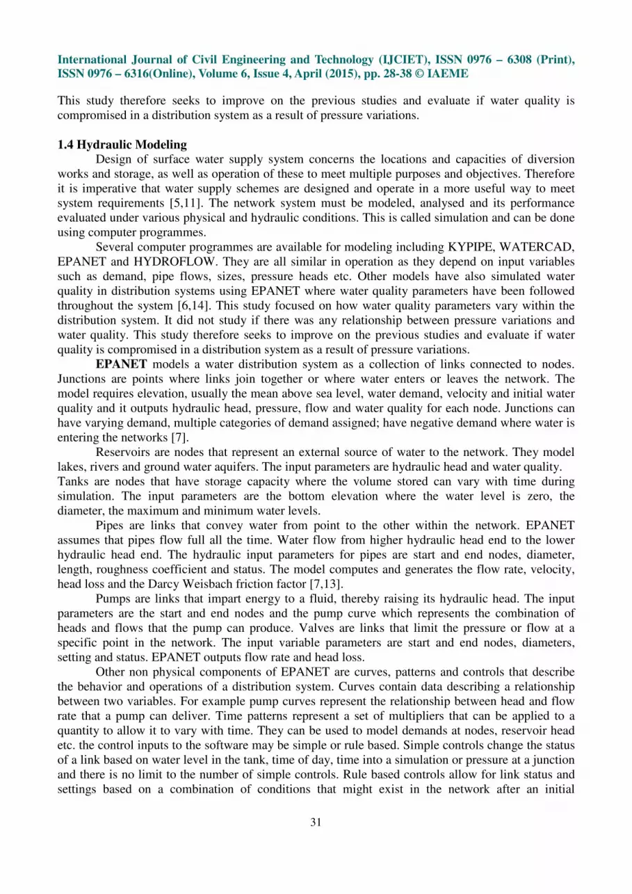
1.4 Hydraulic Modeling

Design of surface water supply system concerns the locations and capacities of diversion

works and storage, as well as operation of these to meet multiple purposes and objectives. Therefore

it is imperative that water supply schemes are designed and operate in a more useful way to meet

system requirements [5,11]. The network system must be modeled, analysed and its performance

evaluated under various physical and hydraulic conditions. This is called simulation and can be done

using computer programmes.

Several computer programmes are available for modeling including KYPIPE, WATERCAD,

EPANET and HYDROFLOW. They are all similar in operation as they depend on input variables

such as demand, pipe flows, sizes, pressure heads etc. Other models have also simulated water

quality in distribution systems using EPANET where water quality parameters have been followed

throughout the system [6,14]. This study focused on how water quality parameters vary within the

distribution system. It did not study if there was any relationship between pressure variations and

water quality. This study therefore seeks to improve on the previous studies and evaluate if water

quality is compromised in a distribution system as a result of pressure variations.

EPANET models a water distribution system as a collection of links connected to nodes.

Junctions are points where links join together or where water enters or leaves the network. The

model requires elevation, usually the mean above sea level, water demand, velocity and initial water

quality and it outputs hydraulic head, pressure, flow and water quality for each node. Junctions can

have varying demand, multiple categories of demand assigned; have negative demand where water is

entering the networks [7].

Reservoirs are nodes that represent an external source of water to the network. They model

lakes, rivers and ground water aquifers. The input parameters are hydraulic head and water quality.

Tanks are nodes that have storage capacity where the volume stored can vary with time during

simulation. The input parameters are the bottom elevation where the water level is zero, the

diameter, the maximum and minimum water levels.

Pipes are links that convey water from point to the other within the network. EPANET

assumes that pipes flow full all the time. Water flow from higher hydraulic head end to the lower

hydraulic head end. The hydraulic input parameters for pipes are start and end nodes, diameter,

length, roughness coefficient and status. The model computes and generates the flow rate, velocity,

head loss and the Darcy Weisbach friction factor [7,13].

Pumps are links that impart energy to a fluid, thereby raising its hydraulic head. The input

parameters are the start and end nodes and the pump curve which represents the combination of

heads and flows that the pump can produce. Valves are links that limit the pressure or flow at a

specific point in the network. The input variable parameters are start and end nodes, diameters,

setting and status. EPANET outputs flow rate and head loss.

Other non physical components of EPANET are curves, patterns and controls that describe

the behavior and operations of a distribution system. Curves contain data describing a relationship

between two variables. For example pump curves represent the relationship between head and flow

rate that a pump can deliver. Time patterns represent a set of multipliers that can be applied to a

quantity to allow it to vary with time. They can be used to model demands at nodes, reservoir head

etc. the control inputs to the software may be simple or rule based. Simple controls change the status

of a link based on water level in the tank, time of day, time into a simulation or pressure at a junction

and there is no limit to the number of simple controls. Rule based controls allow for link status and

settings based on a combination of conditions that might exist in the network after an initial



32

hydraulic state of the system is computed. For example a set of rules that shut down a pump and

opens a bypass valve when the level in the tank exceeds a certain level.

EPANET’s hydraulic simulation model computes junction heads and link flows for a fixed

set of reservoir levels, tanks levels and water demand over a suction of points in time. These

parameters are updated from one time step to another according to prescribed time patterns, while

tank levels are updated using the current flow solution.

The solution for head and flows at a particular point in time involves solving the conservation

of flow at each junction and the head loss relationship across each link in the network through a

process called hydraulic balancing. The process uses an iterative technique to solve the non linear

equations involved. The hydraulic time step for the extended time simulation is set by the user with

one hour being the default.

2. MATERIALS AND METHODS

Kimilili Water Supply network is divided into 5 zones for purposes of smooth operation and

maintenance. Pressure and flow measurements were carried out at each of the 33 nodes representing

the 5 different zones. The measurements were done during peak periods (5am-8am), (12.00-200) pm

and (5-9pm) which corresponded to the simulation period. This period was used as it represented

critical water consumption hours when consumers are either preparing for work in the morning,

preparing for lunch or are back in the evening and preparing for dinner. Measurements were done

using Ultrasonic Flow meter (Portaflow C) type FSC-1/FLD1.

The following was the general procedure used for pressure and flow measurement process at all the

selected points within the 5 zones of the distribution system.

• Power the Portaflow device on

• Input pipe specifications i.e. outer diameter, pipe materials and wall thickness

• Input fluid properties i.e. type of fluid and viscosity

• Enter the name of the site where measurement is being performed

• Outer diameter of the pipe ranges from 13mm to 6000mm, wall thickness ranges from 0.1mm

to 100mm

• Enter lining material for the pipe i.e. tar epoxy, mortar, Rubber, Teflow, Pyrex glass, Pvc etc

• Select sensor monitoring method V or Z method. V method is generally selected (for

diameters upto 300mm) while Z Method is used where ample space is not provided, high

turbidity occurs, there is weak receiving waveform and thick scale is deposited on the pipe

internal surface.

• Select the kind of sensor i.e. FLD12/FSD12

• Select the location for mounting the detector which should meet the following conditions:

• There is a straight pipe portion of 10D or more on the upstream side and that of 5D or more on

the downstream side

• There are no factors to disturb the flow (such as pump and valve) within about 30D of the

upstream side. (JEMIS-032)

• Pipe is always filled with fluid. Neither air bubbles nor foreign materials are contained in the

fluid.

• There is an ample maintenance space around the pipe to which the detector is to be mounted

• Avoid mounting the detector near a deformation, flange or welded part of the pipe.

• For a horizontal pipe, mount the detector within ±45° of the horizontal plane. For a vertical

pipe, it can be mounted at any position on the outer circumference



33

• Mount sensor: wipe off contaminates from the transmitting surface of the sensor and sensor

mounting surface of the pipe. Apply the silicone grease on the transmitting surface of the

sensor while spreading it evenly. Film thickness of silicone grease should be about 3mm.

• Start measuring: when wiring, piping settings and mountings of the sensor are completed, start

the measurement. The contents displayed on the measurement screen are; instantaneous flow,

instantaneous flow velocity, integrated flow rate, analog output and analog input.

Sample Display on the Portaflow-C device

Hydraulic Modeling

EPANET’s hydraulic simulation model computes junction heads and link flows for a fixed

set of reservoir levels, tank levels, and water demands over a succession of points in time. From one

time step to the next reservoir levels and junction demands are updated according to their prescribed

time patterns while tank levels are updated using the current flow solution.

The solution for heads and flows at a particular point in time involves solving simultaneously

the conservation of flow equation for each junction and the head loss relationship across each link in

the network. This process, known as “hydraulically balancing” the network, requires using an

iterative technique to solve the nonlinear equations involved. EPANET employs the “Gradient

Algorithm” for this purpose.

The general procedure for running a hydraulic simulation model involves the following:

• Creating Project defaults such as Identification labels for junctions, reservoirs, Tanks, Pipes,

Pumps, Valves, Patterns, Curves and ID increments

• Drawing the network i.e. pipes, nodes, junctions

• Setting object properties such as x, y coordinates, elevations, base demands etc, hydraulic

properties

• Running a single period analysis to indicate hydraulic properties at a given time



34

• Running an extended period analysis –to make a network more realistic we create a time

pattern that makes demands at nodes vary in periodic way over the course of a day for example

3 hours pattern step makes demand change at eight different times of the day.

• Create a pattern editor with multipliers to simulate demand variations at different times of the

day

3. RESULTS AND DISCUSSION

Simulation Results in terms of Pressure for 10 nodes selected from the 5 zones were analyzed

and compared with the actual measured data. Below is a brief of the findings:

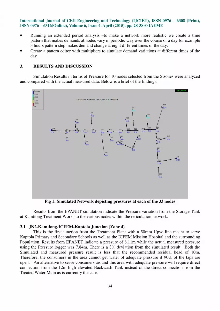
Fig 1: Simulated Network depicting pressures at each of the 33 nodes

Results from the EPANET simulation indicate the Pressure variation from the Storage Tank

at Kamtiong Treatment Works to the various nodes within the reticulation network.

3.1 JN2-Kamtiong-ICFEM-Kaptola Junction (Zone 4)

This is the first junction from the Treatment Plant with a 50mm Upvc line meant to serve

Kaptola Primary and Secondary Schools as well as the ICFEM Mission Hospital and the surrounding

Population. Results from EPANET indicate a pressure of 8.11m while the actual measured pressure

using the Pressure logger was 7.84m. There is a 3% deviation from the simulated result. Both the

Simulated and measured pressure result is less that the recommended residual head of 10m.

Therefore, the consumers in the area cannot get water of adequate pressure if 90% of the taps are

open. An alternative to serve consumers around this area with adequate pressure will require direct

connection from the 12m high elevated Backwash Tank instead of the direct connection from the

Treated Water Main as is currently the case.



35

Fig 2: Pressure Distribution within the network

Fig 3: EPANET Simulated Pressure Compared to Actual Measured Pressure

3.2 JN8-Kamusinga Girls School-(Zone 4)

Results as simulated from EPANET indicate that there is a pressure of 17.02 m and the actual

field pressure as measured was 15.5m. Thus there is a deviation of about 8.9%. The pressure here is

adequate as it is above the required minimal residual head of 10m. The significant deviation can be

attributed to the aged status of the pipeline which has resulted in scaling and increased friction factor.

3.3 JN10-Friends School Kamusinga-(Zone 2)

The line that serves Friends School Kamusinga was identified as JN10 and pressure

measurements were done within the School Compound. Pressure measured was 13m while the

EPANET results indicate an ideal situation of 15m pressure. The variation was attributed to an

online abstraction by the Western Kenya Police Training College located adjacent to the School.

Nevertheless the pressure is enough for the school.

3.4 JN17-Sirende Junction-(Zone 2)

This node is located on the South Eastern end of the Supply area. It one of the nodes further

away from the Treatment Works and also on the lower elevations compared to the Treatment Plant.

The Pressure as measured at this node was 18.56m while the EPANET results indicate that the

pressure should be 20.03m. The Pressures in this part of the network are excessive and consumers



36

complained of water hammer in their taps. This has led to leakages along the line which lead to high

levels of Non Revenue Water as corroborated by the Water Utility Technical staff. It is

recommended that a break Pressure Tank of 10m3 be placed at about 2km to Sirende Junction to try

and contain the excessive pressures witnessed in the pipeline.

3.5 JN20-Water Offices-(Zone 1)

Pressure measurement at the Water Utility offices indicated as pressure of 26m at the Tap

while EPANET simulation indicated a pressure of 23.05m. This node had measured pressures

exceeding simulated results. This was attributed to the reduction in size of the pipeline from 75mm at

the off take to 38mm at the Water offices. This has lead to leakages through the tap it was

recommended that a new pipeline of 75mm be laid to replace the 38mm which would reduce the

pressure to manageable levels. It was also recommended that Pressure Reducing valve be installed

on the line.

3.6 JN12-Nabwana Estate Line-(Zone 1)

This Zone is at the Central Business District of Kimilili Town and consumers are mostly

commercial units as well as residential homes. Measured pressure was 15.43m while the simulated

EPANET Result was 17.76m indicating that the actual pressure in the field was lower than the ideal

one. Generally pressure in this zone is fine and consumers are happy since water of significant

pressure is received even on 3 story buildings within the town. There is however rapid growth and

connections onto the network. It is further recommended that a section valve be placed just after JN

11 to regulate flows based on the demands.

3.7 JN23-Matili R.C Church line-(Zone 3)

Pressure measured at this node was 30m while EPANET indicated a result of 34.7m. This

line is 50mm Upvc and has very few connections. Thus very few consumers use the line which

results in pressure build up. A connection to Matili Technical Training Institute needs to be effected

to reduce the excessive pressure within the line.

3.8 JN26-Bahayi line-(Zone 3)

This node recorded actual pressure of 34.5m while EPANET indicated a pressure of 39.48m.

These are excessive pressures and a pressure reducing valve is proposed on each of the pipeline

junction to avert bursts and leakages that tare frequent in this zone.

3.9 JN27-Misikhu Junction-(Zone 5)

Actual Measured pressure at this junction was 23.5m while EPANET Indicated a Pressure of

23.05m. This is the main junction from where a line goes to Namarambi Weigh Bridge and the other

line proceeds towards Lugulu through Tete. It eventually feeds Mikuva and Lugulu market.

3.10 JN33-Mikuva line-(Zone 5)

This node is on the pipeline branching from the Main line at Lugulu Market. It had an actual

pressure of 20.4m while the simulated pressure through EPANET was 24.03m indicating a deviation

of about 4m. The area has quite enough pressure bearing in mind that is among the zones with lower

elevations within the network. The Main improvement recommended on this line is to extend the

pipeline from Mikuva to some 3km towards Siloi area to help even out pressure build up.



37

4. CONCLUSION AND RECOMMENDATIONS

The Study was aimed at simulating the Variation of Pressure within the 5 zones of Kimilili

Water Reticulation network to find out how it is distributed within the zones. Field measurements

were also carried out and compared with the simulated data. In can therefore be concluded as

follows:

• Less than 12% of the nodes in the entire Kimilili Water reticulation have residual pressures

less than the recommended minimum of 10m. These areas are mainly around the Treatment

Plant owing to their elevation orientation. Therefore to serve these consumers with adequate

pressure , it is recommended that a dedicated line be laid from the Backwash Tank located at

the Treatment Works

• Pressure varies within the network and generally increases as one move further away from the

Treatment Works as a result of the buildup.

• More than 80% of the network receives pressures above 16m which requires Break pressure

tanks and Pressure reducing Valves to prevent excessive water hammer in the taps.

• Simulated Pressure results from EPANET are generally higher than actual field results due to

the aging nature of the network.

• EPANET Software is a useful tool for extended period simulation which should be embraced

by Water Utilities especially in the Developing Countries to simulate and predict Hydraulic

Parameters thereby manage efficiently the Water distribution networks.

• The Study utilized EPANET simulation to visualize pressure variations in the Water

reticulation network. Further research can be done using the same software but to establish if

there is any relation between pressure variation and levels of Contaminants ingress in the

network and also relate it to water age.

ACKNOWLEDGEMENTS

The Authors are grateful to Masinde Muliro University of Science and Technology,

Kakamega, Kenya for their cooperation and encouragement to carry out the Study. We are also

grateful to the technical staff of Nzoia Water and Sanitation Company (Nzowasco) for their

dedicated technical support.

REFERENCES

1. Oklahoma Department of Environment and Quality Manual, (2008).

2. Environmental Protection Agency Manual (2008)

3. Hickey, H (FEMA) ,(2008):Water Supply Systems and Evaluation Methods Vol.I.: Water

Supply Systems concept

4. Cheung, P. B., Van Zyl, J.E. & Reis, L.F.R. (2005): Extension of Epanet for Pressure Driven

Demand Modelling in Water Distribution System CCWI2005 Water Management for the

21st Century, Exeter, UK.

5. Kapelan, Z., Savic,D.A,.and Walters,G.A (2000): Inverse Transient analysis in pipe networks

for leakage detection and roughness calibration, proceedings of water network modeling for

optimal design and management, Exeter, UK.

6. Senyondo,(2000).: Master’s Thesis on “Optimization of Water Distribution Network using

EPANET”

7. Rossman A. L. (2000) EPANET Users’ Manual. National Risk Management Laboratory.

United States Environmental Protection Agency, Ohio.



38

8. Ang, W. K. & Jowitt P.W. (2006): Solution for water distribution systems under pressure-

deficient conditions. Journal of Water Resources Planning and Management, Volume 132,

issue (3): pp175-182.

9. Chandapillai, J. (1991): Realistic Simulation of Water Distribution Systems. Journal of

Transportation Engineering, Volume 117, Issue (2):pp 258-263.

10. Clement J.,Cheung et al, (2004).: Predictive Models for Water Distribution Systems,

Distribution Network Design using Differential Evolution”. Journal of distribution systems:

A UK case study”, Copernicus Publications, Drink, UK

11. Hayuti M. H., Burrows R. & Naga D. (2007): Modelling water distribution systems with

deficient pressure. Water Management, 160: 215-224.

12. Hickey, H (FEMA) ,(2008):Water Supply Systems and Evaluation Methods Vol.I.: Water

Supply Systems concept

13. Machell,J., Mounce, S. R. and Boxall, J. B(2004):“Online modelling of water Mays, L.W.

(2004) Water supply systems security. McGraw-Hill. Modelling “Intermittent Water Supply

Systems with Epanet”. 8th annual conference

14. Nyende-Byakika, S. (2011) Modelling of Pressurised Water Supply Networks that may

exhibit Transient Low Pressure-Open Channel Flow Conditions. PhD Thesis. Vaal University

of Technology. Vanderbijlpark. South Africa.

15. Nyende-Byakika, S., Ngirane-Katashaya G. & Ndambuki, J.M. (2010) Behaviour of stretched

water supply networks. Nile Water Science and Engineering Journal, 3(1).

16. Ozger S. (2003) A semi-pressure driven approach to reliability assessment of water

distribution networks. PhD Thesis. Arizona State University.

17. Sarbu, I and Valea, S.E (2011): “Nodal analysis of looped water Issue 3, Volume 5, Pp 452-

460, 2011.

Documents

SIMULATION OF PRESSURE VARIATIONS WITHIN KIMILILI WATER SUPPLY SYSTEM USING EPANET