Embed Size (px)
Citation preview

arX
iv:c
ond-
mat
/000
4416
v1 [
cond
-mat
.sup
r-co
n] 2
5 A
pr 2
000
EPJ manuscript No.(will be inserted by the editor)
Small Bipolarons in the 2-dimensional Holstein-Hubbard Model
I The Adiabatic Limit
L. Proville a and S. Aubry
Laboratoire Leon Brillouin (CEA-CNRS), CEA Saclay 91191-Gif-sur-Yvette Cedex, France
Received: December 10 1998 / Revised: February 1, 2008
Abstract. The spatially localized bound states of two electrons in the adiabatic two-dimensional Holstein-
Hubbard model on a square lattice are investigated both numerically and analytically. The interplay
between the electron-phonon coupling g, which tends to form bipolarons and the repulsive Hubbard inter-
action υ ≥ 0, which tends to break them, generates many different ground-states. There are four domains
in the g, υ phase diagram delimited by first order transition lines. Except for the domain at weak electron-
phonon coupling (small g) where the electrons remain free, the electrons form bipolarons which can 1)
be mostly located on a single site (small υ, large g); 2) be an anisotropic pair of polarons lying on two
neighboring sites in the magnetic singlet state (large υ, large g); or 3) be a ”quadrisinglet state” which
is the superposition of 4 electronic singlets with a common central site. This quadrisinglet bipolaron is
the most stable in a small central domain in between the three other phases. The pinning modes and the
Peierls-Nabarro barrier of each of these bipolarons are calculated and the barrier is found to be strongly
depressed in the region of stability of the quadrisinglet bipolaron.
PACS. 71.10.Fd Lattice fermion models (Hubbard model, etc.) – 71.38.+i Polarons and electron phonon
interactions – 74.20.Mn Nonconventional mechanisms (spin fluctuations, polarons and bipolarons, res-
onating valence bond model, anyon mechanism, marginal Fermi liquid, Luttinger liquid, etc.) – 74.25.Jb
Electronic structure
a Present Address: DAMTP Cambridge University, Cam-
bridge, CB3 9EW, UK
1 Introduction
The standard BCS theory of superconductivity [1] holds
for a system of noninteracting electrons weakly coupled

2 L. Proville, S. Aubry: Small Bipolarons in the 2-dimensional Holstein-Hubbard Model
to a quantum field of phonons. It has been well-known for
several decades that when the electron-phonon coupling
increases too much, the BCS theory breaks down because
of lattice instabilities [2]. As a consequence, rather low
critical temperatures (≈ 30K) were predicted as the upper
bound for real BCS superconductors [3]. Many theories
have subsequently been developed to describe the strong
coupling regime with the hope to predict the existence
of non-BCS superconductors with high critical tempera-
ture. After the discovery by Bednorz and Muller [4,5,6]
of cuprate materials, which can be superconducting at
temperatures as high as 100K or more, the bipolaron ap-
proach (among others) regained much interest [7].
Since Landau [8], it has been acknowledged that a sin-
gle electron (or equivalently a pair of noninteracting elec-
trons coupled to a deformable classical field) may localize
in the potential created self-consistently by a deformation
of the field. The resulting object is called ”polaron” for one
electron or ”bipolaron” for two electrons. The bipolaron
theory of Alexandrov et al.[9] involves small bipolarons
which are pairs of electrons with opposite spins, sharply
localized at single sites of the lattice. Actually, because
the phonons are quantum, these bipolarons are hard-core
bosons that could condense in a superfluid state. For mod-
els in two dimensions and more, bipolarons exist only
when the electron-phonon coupling is large enough [10],
and they are always sharply localized as small bipolarons
when the interactions are local. Thus, taking physically re-
alistic parameters for the model, the effective mass of the
bipolarons becomes so huge (quasi-infinite) that it seems
quite unreasonable to expect the bipolarons to become
superfluid at a non-negligible temperature. This aspect
of the problem has been emphasized recently in ref.[11].
However, the argument used by these authors was based
on standard considerations that did not take into account
the effect of mass reduction we shall discuss in this and a
subsequent paper [17].
Indeed, in realistic physical models, the characteristic
energy of the bare electrons is usually a few eV and is
much larger than the phonon energies which is at most
about a tenth of an eV. As a result, the quantum fluctu-
ations of the phonons become generally negligible as soon
as the electron-phonon coupling is strong enough to gen-
erate bipolarons. Then the potential interactions between
the bipolarons are much larger than their quantum kinetic
energy. In that situation, the many bipolaron structures
should be well described by an effective Ising pseudospin
Hamiltonian, predicting an insulating Bipolaron Charge
Density Wave at low temperature [12,13,14].
However, there might exist special and exceptional sit-
uations where the effective mass of the bipolarons is not
quasi-infinite but becomes small enough so that they pos-
sibly condense into a superfluid state. The smaller the
bipolaron mass is, the higher the critical temperature should
be. As conjectured in ref.[15] and [16], this situation might
be produced by a well-balanced interplay between the
bare electronic kinetic energy, the electron-phonon cou-
pling and the direct electron-electron repulsion. The aim
of this paper is to study this interplay in the simplest

L. Proville, S. Aubry: Small Bipolarons in the 2-dimensional Holstein-Hubbard Model 3
Holstein-Hubbard (HH) model where these interactions
are present.
This first paper is devoted to the study of a single bipo-
laron in the HH model in the adiabatic limit, assuming
classical phonons. Obviously the assumption that there
are no quantum phonon fluctuations does not allow su-
perfluid states (with many electrons). In the next paper
[17], the quantum phonon correction to the adiabatic case
will be studied. There, it will be shown that in some re-
gions of the parameter space, there is indeed a drastic
reduction of the quantum bipolaron’s effective mass due
to quantum resonances between several almost degenerate
adiabatic bipolaron structures. A large part of the scien-
tific material of these two papers can be already found (in
French) in the PhD dissertation of one of us [18].
Some numerical studies of the bipolarons in the one-
dimensional adiabatic HH model, were already presented
in ref.[19] (as well as few preliminary studies in two dimen-
sions). Bipolarons always exist in one-dimensional mod-
els as expected, but when the Hubbard term υ increases
from zero, a first order transition occurs between the single
site bipolaron (S0) and a bipolaron (S1) composed of two
bounded polarons on two neighboring sites in a magnetic
singlet state. It was observed that the classical mobility of
the bipolaron (assuming the lattice dynamics is classical)
was significantly enhanced in the vicinity of this transi-
tion. Owing to the presence of the Hubbard term, quite
small bipolarons could become nevertheless highly mobile
over hundreds of lattice spacings.
The behavior of the bipolaron in the two-dimensional
case is quite different from the one-dimensional case. Al-
though it does not describe precisely the CuO2 planes
of cuprates [6], it might exhibit similar features as more
realistic models. In two-dimensional models with local in-
teractions, the bipolarons exist only for a large enough
electron-phonon coupling and are always sharply localized
(small bipolarons). We numerically calculate these bipo-
larons by using a continuation method of these solutions
from the anti-integrable limit [20], where the electronic
transfer integral is zero.
The ground state of the bipolarons in this limit can be
easily found and consists of either a bipolaron localized at
a single site (S0) or of two uncoupled polarons at arbitrary
different sites, but there are many other states with larger
energy that are combinations of singlet states (multisin-
glets). Many of these bipolaron states can be continued
when the transfer integral varies from zero and their en-
ergies can be compared. Although the bipolaron (S0) or
the singlet bipolaron (S1), persist with the lowest energy
in large parts of the phase diagram, it is found that a
quadrisinglet state (QS) becomes the ground-state in an
intermediate regime of parameters.
We show that we can reproduce quite accurately the
same phase diagram by choosing variational wave func-
tions for the electrons made from simple combinations of
exponentials reproducing the main characteristic of the
spin structure of the bipolaron. ( This is an extension of
the variational method used in ref.[21]). Further exten-

4 L. Proville, S. Aubry: Small Bipolarons in the 2-dimensional Holstein-Hubbard Model
sions could be developed later for the many-body prob-
lem.
We investigate the properties of all the obtained so-
lutions by calculating their binding energies, their pin-
ning and breathing modes and also their Peierls-Nabarro
energy barrier. We find a substantial softening of their
pinning (and breathing) modes and a sharp depression
of the PN energy barrier in the region where the (QS)
bipolaron becomes the ground-state. Although the classi-
cal mobility of the bipolarons never becomes as large as
in the one-dimensional case [19], it is sufficient to favor
a good quantum mobility [17] in a specific region of the
phase diagram.
2 The Model
To keep in mind the physical magnitude of the dimen-
sionless parameters involved in our reduced model, let us
first write the Holstein-Hubbard Hamiltonian with all its
parameters measured in the original physical units:
H = − T∑
<i,j>,σ
C+i,σCj,σ +
∑
i
hω0(a+i ai)
+∑
i
gni(a+i + ai) +
∑
i
υni,↑ni,↓ (1)
The electrons are represented by the standard fermion
operators C+i,σ and Cj,σ at site i with spin σ =↑ or ↓. Then
T is the transfer integral of the electrons between nearest
neighbor sites < i, j > of the lattice. In physical systems,
its order of magnitude is usually measured in eV.
a+i and ai are standard creation and annihilation bo-
son operators of phonons. hω0 is the phonon energy of a
dispersionless optical phonon branch with order of mag-
nitude a tenth of an eV at most.
g is the constant of the on-site electron-phonon cou-
pling which may physically range from zero to a fraction of
an eV. The on-site electron-electron interaction is repre-
sented by a Hubbard term with positive coupling υ which
may range physically from negligible to large values of the
order of 10 eV.
Choosing E0 = 8g2/hω0 as the energy unit and intro-
ducing the position and momentum operators:
ui =hω0
4g(a+
i + ai) (2)
pi = i2g
hω0(a+
i − ai) (3)
we obtain the dimensionless Hamiltonian:
H =∑
i
(
1
2u2
i +1
2uini + Uni↑ni↓
)
− t
2
∑
<i,j>,σ
C+i,σCj,σ
−γ2
∑
i
p2i (4)
The parameters of the system are now:
E0 = 8g2/hω0 U =υ
E0t =
T
E0γ =
1
4(hω0
2g)4
(5)
The parameter γ measures how ”quantum” is the lat-
tice. The BCS theory requires g << hω0: that is, large γ.
We are interested in the opposite regime of strong electron-
phonon coupling: that is, g larger than the phonon energy
hω0. Then γ becomes small.
Thus the adiabatic approximation, which is simply ob-
tained by taking γ = 0, becomes valid in the strong elec-
tron phonon regime. We shall assume this condition in

L. Proville, S. Aubry: Small Bipolarons in the 2-dimensional Holstein-Hubbard Model 5
this first paper. Then {ui} commutes with the Hamilto-
nian and can be taken as a scalar variable. For a given set
of {ui}, the adiabatic Hamiltonian
Had =∑
i
(
1
2u2
i +1
2uini + Uni↑ni↓
)
− t
2
∑
<i,j>,σ
C+i,σCj,σ
(6)
commutes with the total spin of the system.
Thus, the eigenstates of a system with two electrons
are either nondegenerate singlet states or three-fold degen-
erate triplet states. The wavefunction of the singlet state
has the form
|Ψ >=∑
i,j
ψi,jC+i,↑C
+j,↓|∅ > (7)
where |∅ > is the vacuum (no electrons in the system) and
ψi,j = ψj,i is normalized
∑
i,j
|ψi,j |2 = 1 (8)
on the 2D lattice (ZD)2 (D = 2 being the lattice di-
mension we consider in this paper). The wave function of
the triplet state (oriented with the spin +1 in order to fix
the ideas), has the form
|Ψ >T =∑
i,j
ψTi,jC
+i,↑C
+j,↑|∅ > (9)
where ψTi,j = −ψT
j,i is normalized and antisymmetric.
Actually, the singlet wave and the triplet functions which
are eigenstates of the adiabatic Hamiltonian (6) both yield
the same eigen-equation for their components ψi,j or ψTi,j
− t
2∆ψi,j +
(
1
2(ui + uj) + Uδi,j
)
ψi,j = Fel({ui})ψi,j
(10)
where ∆ is the discrete Laplacian operator in the 2D lat-
tice (ZD)2 defined as (∆Ψ)i =∑
j:i Ψj where j ∈ (ZD)2
are the nearest neighbors of i ∈ (ZD)2.
Unlike the singlet states, the eigenenergies of the triplet
states do not depend on the Hubbard term U since ψTi,i = 0
and thus are just the same as for noninteracting electrons.
Taking into account that in our model, the transfer in-
tegrals with amplitude t > 0 connect only the nearest
neighbor sites, it is straightforward to check that the sin-
glet state defined as ψi,j = |ψTi,j | always has less energy
than the triplet state with wave function {ψTi,j}. As a re-
sult, the ground-state of our system is necessarily a singlet
state with the form (7).
The energy of (6) depends on {ψi,j} and {ui} as
F ({ψi,j}, {ui}) =∑
i
(
1
2u2
i +ui
2ρi + U |ψi,i|2
)
− t
2< ψ|∆|ψ > (11)
where the electronic density at site i is
ρi =∑
j
(|ψi,j |2 + |ψj,i|2) (12)
Extremalizing F ({ψi,j}, {ui}) with respect to the nor-
malized electronic state {ψi,j} and the displacements {ui}
yields the set of coupled equations (10) and
ui +ρi
2= 0 (13)
Fel({ui}) is an eigenenergy of two interacting electrons
in the potential generated by the lattice distortion {ui}.
Using eq.13, the extrema of eq.11 are those of the varia-
tional energy

6 L. Proville, S. Aubry: Small Bipolarons in the 2-dimensional Holstein-Hubbard Model
Fv({ψi,j}) =∑
i
(
−1
8ρ2
i + U |ψi,i|2)
− t
2< ψ|∆|ψ >
(14)
for ψi,j normalized and where ρi is given by eq.12. Then,
it follows that
− t
2∆ψi,j +
(
−1
4(ρi + ρj) + Uδi,j
)
ψi,j = Felψi,j (15)
and also that the solutions of this equation, the energy of
the system is
Fv({ψi,j}) = Fel +1
8
∑
i
ρ2i (16)
3 Numerical Continuations of Bipolarons
from the Anti-Integrable Limit
3.1 Bipolarons in the Anti-Integrable Limit
In the anti-integrable limit t = 0, the adiabatic ground-
state for two electrons is easily found. For U ≤ 1/4, it
consists of a pair of electrons localized at a single site i.
This is the standard small bipolaron known in the litera-
ture, denoted (S0) (see fig.1). For a bipolaron at site i, its
electronic wave function is
|Ψ >= C+i,↑C
+i,↓|∅ > (17)
and its energy is Fv = U − 1/2.
When U ≥ 1/4, the ground-state consists of two un-
bound polarons localized at arbitrary different sites i and
j and with arbitrary spins. It is thus degenerate and its
energy Fv = −1/4 is independent of the Hubbard interac-
tion. When sites i and j are nearest neighbors, we define
the bipolaron (S1) [15,16] (see fig.1) with electronic wave
function
|Ψ >=1√2(C+
i,↑C+j,↓ + C+
j,↑C+i,↓)|∅ > (18)
where i and j are nearest neighbor sites.
Since a single polaron has the electronic spin 1/2, when
the transfer integral t is small but not zero, a standard
perturbation theory yields an antiferromagnetic exchange
coupling 2t2/U between the two spins of the uncoupled
neighboring polarons. When the spins are chosen in the
singlet state represented by eq.18, these two polarons have
the energy Fv ≈ −1/4 − t2/U . When they are not lo-
cated at nearest-neighbor sites but at the lattice distance
n, perturbation theory to order n yields an antiferromag-
netic exchange coupling proportional to U(t/U)2n. Thus,
for t << U , the minimum energy is obtained for nearest
neighbor bipolarons in the singlet magnetic state (S1). It
is maximum when U is close to and above 1/4, just when
(S1) becomes of lower energy than (S0). For t fixed, it de-
creases to zero when U increases. This binding energy also
vanishes in the anti-integrable limit t. Unlike bipolaron
(S0), bipolaron (S1) breaks the square lattice symmetry
and is oriented either in the x direction or the y direction.
When t is not very small, the spatial extension of the
polarons goes significantly beyond single sites, and it is
not obvious that a low-order perturbation theory holds.
The true ground state might not be obtained by contin-
uation of the solutions (S0) or (S1). There are infinitely
L. Proville, S. Aubry: Small Bipolarons in the 2-dimensional Holstein-Hubbard Model 7
many other bipolaron states at t = 0 (solutions of eq.10),
which have been classified in appendix (A) 1. Some of
them are not very different in energy and could compete to
become the true bipolaron ground-state when t increases.
Therefore, it becomes useful to test the ground-state of
the bipolaron at t 6= 0 among the extrema of eq.14 that
are obtained by continuation from those calculated in the
anti-integrable limit at t = 0.
It is of course impossible to continue and to test nu-
merically the energy of all the solutions of eqs.10 at t = 0.
The study of appendix (A) shows that the binding energy
of the bipolarons is non-negligible only when the total
number Ns of occupied sites is not too large. The non-
connected bipolaron states are discarded because at t = 0
they always have more energy than their connected com-
ponent with the smallest energy, and at t 6= 0, their ab-
sence of connectivity is not favorable for gaining energy
from the electronic kinetic energy term with amplitude t.
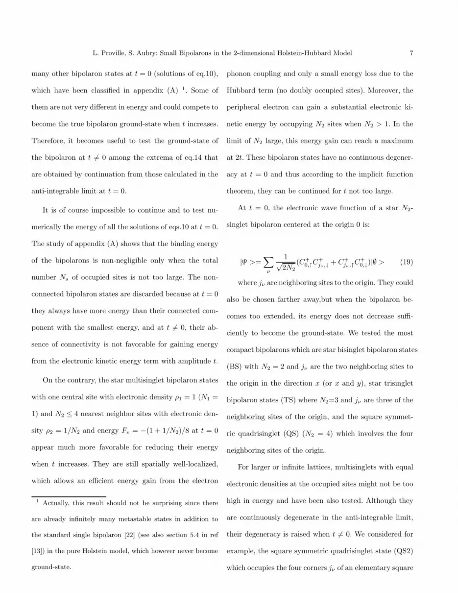
On the contrary, the star multisinglet bipolaron states
with one central site with electronic density ρ1 = 1 (N1 =
1) and N2 ≤ 4 nearest neighbor sites with electronic den-
sity ρ2 = 1/N2 and energy Fv = −(1 + 1/N2)/8 at t = 0
appear much more favorable for reducing their energy
when t increases. They are still spatially well-localized,
which allows an efficient energy gain from the electron
1 Actually, this result should not be surprising since there
are already infinitely many metastable states in addition to
the standard single bipolaron [22] (see also section 5.4 in ref
[13]) in the pure Holstein model, which however never become
ground-state.
phonon coupling and only a small energy loss due to the
Hubbard term (no doubly occupied sites). Moreover, the
peripheral electron can gain a substantial electronic ki-
netic energy by occupying N2 sites when N2 > 1. In the
limit of N2 large, this energy gain can reach a maximum
at 2t. These bipolaron states have no continuous degener-
acy at t = 0 and thus according to the implicit function
theorem, they can be continued for t not too large.
At t = 0, the electronic wave function of a star N2-
singlet bipolaron centered at the origin 0 is:
|Ψ >=∑
ν
1√2N2
(C+0,↑C
+jν ,↓ + C+
jν ,↑C+0,↓)|∅ > (19)
where jν are neighboring sites to the origin. They could
also be chosen farther away,but when the bipolaron be-
comes too extended, its energy does not decrease suffi-
ciently to become the ground-state. We tested the most
compact bipolarons which are star bisinglet bipolaron states
(BS) with N2 = 2 and jν are the two neighboring sites to
the origin in the direction x (or x and y), star trisinglet
bipolaron states (TS) where N2=3 and jν are three of the
neighboring sites of the origin, and the square symmet-
ric quadrisinglet (QS) (N2 = 4) which involves the four
neighboring sites of the origin.
For larger or infinite lattices, multisinglets with equal
electronic densities at the occupied sites might not be too
high in energy and have been also tested. Although they
are continuously degenerate in the anti-integrable limit,
their degeneracy is raised when t 6= 0. We considered for
example, the square symmetric quadrisinglet state (QS2)
which occupies the four corners jν of an elementary square

8 L. Proville, S. Aubry: Small Bipolarons in the 2-dimensional Holstein-Hubbard Model
of the lattice. One of its degenerate wave functions is
|Ψ >=∑
ν 6=ν′
1√8C+
jν ,↑C+jν′ ,↓|∅ > (20)
with energy Fv = −1/8
3.2 Numerical Technique of Continuation
The most efficient numerical techniques for the continu-
ation of solutions of sets of equations as a function of a
parameter, are usually based on a Newton method. For ex-
ample, such techniques were developed efficiently for cal-
culating discrete breathers [23]. In our case to calculate
accurately adiabatic bipolarons on a 2D system, a rea-
sonable size should be 10 × 10. Then calculating the 104
components of ψi,j with a Newton method, requires to
work with huge matrices containing 108 coefficients: that
is, to use a large-memory, fast computer. Actually, smaller
size conventional computers suffice if one uses appropri-
ate techniques needing a much smaller working space. This
technique does not allow to continue all solutions but only
those which are locally stable (in particular, the bipolaron
ground-state) and those that can be made stable by fixing
some spatial symmetries of the bipolaron.
This method is quite simple in its principle. To solve
eq.15 with condition (12), we start from a normalized trial
solution of eq.15, Φ = {φi,j} with φi,j = φj,i, and we
calculate recursively a new normalized trial solution Ψ1 =
T (Φ) = {ψi,j} as
N1ψi,j = − t
2∆φi,j +
(
Uδi,j −∑
k
(φ2i,k + φ2
j,k) −K
)
φi,j
(21)
where N1 is the normalization factor (chosen negative)
and K is some positive constant that we introduce to en-
sure the convergence to a minimum energy state. Actually,
it can be chosen to be zero in the domain of parameter we
study.
We find numerically that for n large enough, Ψn =
T (Ψn−1) and its normalization factor Nn converge to the
limits Ψ and N , respectively. Ψ is a solution of eq.15 with
the condition (12) and for the eigenenergy Fel = N −
K. This solution corresponds to the eigenvector of eq.15
(where ρi and ρj are fixed) associated with the eigenvalue
Fel which is such that Fel −K has the largest modulus. In
principle, the constant K is chosen large enough in order
that Fel is surely the lowest negative eigenvalue: that is,
for the electronic ground-state. One can easily check in the
anti-integrable limit that K = 0 is an appropriate choice
when U < 1/2. Varying one of the model parameters by
small steps, each solution is taken as a trial solution for
the next step. It is easy to determine whether the solution
varies quasicontinuously or discontinuously.
For the solutions in the anti-integrable limit which are
non-degenerate, it can be checked that the hypotheses of
the implicit function theorem, are fulfilled. Thus continu-
ation is in principle possible 2. For those which belong to
a degenerate continuum, the conditions for applying the
implicit theorem are not fulfilled, but when some spatial
2 The implicit function theorem was already used in simi-
lar anti-integrable limits, for example in ref.[24] for polarons
and bipolarons in the original Holstein model or in ref.[25] for
discrete breathers.

L. Proville, S. Aubry: Small Bipolarons in the 2-dimensional Holstein-Hubbard Model 9
x=-y
x
y x=y
S0S1
yx=y
x=-y
x
y
QS
Fig. 1. Schemes of the bipolarons (S0), (S1) and (QS) appearing as possible ground-states
0.00 0.05 0.10 0.15 0.20 0.25 0.30 0.35 0.40U
0.02
0.04
0.06
0.08
0.10
0.12
0.14
t
0.22 0.24 0.26 0.28 0.30U
0.08
00.
085
t
QS
S1S0
extendedstate
S1
S0
Fig. 2. Phase diagram of the bipolaron in the 2D Holstein-Hubbard model in the plane of parameters U and t. There are four
phase domains separated by first order transition lines corresponding to bipolarons (S0), (S1), (QS) and two unbound extended
electrons. Also shown are the limit of metastability of the bipolaron (S0) (dotted line), bipolaron (S1) (dot-dashed line) and
bipolaron (QS) (dashed line). Insert: Magnification of the phase diagram around the triple point involving phases (S0), (S1)
and (QS).
symmetries or some constraints on the solution are fixed,
the degeneracy at t = 0 can lifted and this theorem ap-
plies.
In the anti-integrable limit, only (S0) for U < 1/2 and
(S1) for 0 < U (and (Sn) with n > 0 being the distance
between two polarons) are numerically stable: that is, can
be followed continuously from t = 0 by using algorithm
(21). Actually, we choose as initial solution at t = 0, the
exact bipolaron solutions described above, which are (S0),
(S1), (QS), (BS), (TS) and (QS2). Maintaining by force

10 L. Proville, S. Aubry: Small Bipolarons in the 2-dimensional Holstein-Hubbard Model
the spatial symmetries of the solution at t = 0, the conver-
gence process becomes stable again, and the continuation
of these solutions is feasible.
The main advantage of our method is that it can be
performed on standard computers. Its flaw is that we might
not be able to follow continuously a solution that is mathe-
matically continuable. Actually, rather few bipolaron states
are continuable. In contrast, our method is very reliable for
finding the true bipolaron ground state, because it brings
spontaneously the bipolaron solution to a local minimum
of the variational energy.
Actually, we checked that when there is no symmetry
constrains and independant of the initial trial solution,
in most cases our numerical algorithm converges sponta-
neously toward the same bipolaron state, which then can
be considered as the true bipolaron ground-state. How-
ever, this situation does not occur in the vicinity of the
first order transition lines where we can obtain a few dif-
ferent bipolaron states depending on the initial condition,
but then their energies can be easily compared to find the
ground-state.
3.3 Bipolaron Phase Diagram
The ground-state for a pair of electrons is obtained by
comparing the energies Fv of many bipolarons continued
from the anti-integrable limit (see also [19]). For larger
t, the ground-state corresponds to a pair of electrons ex-
tended over the whole system. There is a first order tran-
sition line, when t becomes smaller, at which the two elec-
trons bind with each other and self-localize into a bipo-
laron. The region below this line is divided into three do-
mains separated by other first-order transition lines. For
U small, the bipolaronic ground-state is (S0). When U in-
creases for t not too large, there is a transition line between
bipolarons (S0) and (S1). For larger t, this transition line
bifurcates at a triple point at t ≈ 0.785 and U ≈ 0.235 into
two first order transition lines which both join the transi-
tion line with the extended states. In between the fork that
is generated, there is a small domain where the bipolaron
(QS) that was initially unstable for t small, recovers its
stability and even becomes the ground-state. Other bipo-
laronic structures continued from the anti-integrable limit
at t = 0 appear as minimum energy states in the domain
shown on fig.2. The (QS) solution can be viewed as a lo-
calized RVB state similar to that proposed by Anderson
some years ago [26] in the pure Hubbard model in 2D as
a theory for superconductivity in cuprates.
In our model, this (QS) bipolaron has the quantum
symmetry (s) because the kinetic energy term is Laplacian-
like. However, the study of appendix (C) in the anti-integrable
limit, suggests that it is close in energy to other states with
quantum symmetry (s′) or (d). Such symmetries could be
favored by slight model variations on the form of the ki-
netic energy.
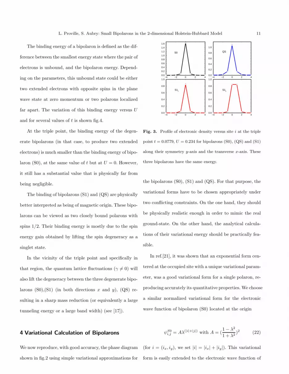
At the triple point, the bipolaronic structure of our
model is degenerate between three states (S0), (S1) and
(QS). Fig.3 shows the profiles of the electronic density
for these three types of bipolaron, which have the same
energy. Interestingly, they extend significantly over only a
few sites, and thus can be called small bipolarons.
L. Proville, S. Aubry: Small Bipolarons in the 2-dimensional Holstein-Hubbard Model 11
The binding energy of a bipolaron is defined as the dif-
ference between the smallest energy state where the pair of
electrons is unbound, and the bipolaron energy. Depend-
ing on the parameters, this unbound state could be either
two extended electrons with opposite spins in the plane
wave state at zero momentum or two polarons localized
far apart. The variation of this binding energy versus U
and for several values of t is shown fig.4.
At the triple point, the binding energy of the degen-
erate bipolarons (in that case, to produce two extended
electrons) is much smaller than the binding energy of bipo-
laron (S0), at the same value of t but at U = 0. However,
it still has a substantial value that is physically far from
being negligible.
The binding of bipolarons (S1) and (QS) are physically
better interpreted as being of magnetic origin. These bipo-
larons can be viewed as two closely bound polarons with
spins 1/2. Their binding energy is mostly due to the spin
energy gain obtained by lifting the spin degeneracy as a
singlet state.
In the vicinity of the triple point and specifically in
that region, the quantum lattice fluctuations (γ 6= 0) will
also lift the degeneracy between the three degenerate bipo-
larons (S0),(S1) (in both directions x and y), (QS) re-
sulting in a sharp mass reduction (or equivalently a large
tunneling energy or a large band width) (see [17]).
4 Variational Calculation of Bipolarons
We now reproduce, with good accuracy, the phase diagram
shown in fig.2 using simple variational approximations for
−4 −2 0 2 40.0
0.2
0.4
0.6
0.8
1.0−4 −2 0 2 4
0.0
0.2
0.4
0.6
0.8
1.0
1.2
1.4
1.6
−4 −2 0 2 40.0
0.2
0.4
0.6
0.8
1.0−4 −2 0 2 4
0.0
0.2
0.4
0.6
0.8
1.0
S0 QS
S1x S1y
Fig. 3. Profile of electronic density versus site i at the triple
point t = 0.0779, U = 0.234 for bipolarons (S0), (QS) and (S1)
along their symmetry y-axis and the transverse x-axis. These
three bipolarons have the same energy.
the bipolarons (S0), (S1) and (QS). For that purpose, the
variational forms have to be chosen appropriately under
two conflicting constraints. On the one hand, they should
be physically realistic enough in order to mimic the real
ground-state. On the other hand, the analytical calcula-
tions of their variational energy should be practically fea-
sible.
In ref.[21], it was shown that an exponential form cen-
tered at the occupied site with a unique variational param-
eter, was a good variational form for a single polaron, re-
producing accurately its quantitative properties. We choose
a similar normalized variational form for the electronic
wave function of bipolaron (S0) located at the origin
ψS0i,j = Aλ(|i|+|j|) with A = (
1 − λ2
1 + λ2)2 (22)
(for i = (ix, iy), we set |i| = |ix| + |iy|). This variational
form is easily extended to the electronic wave function of

12 L. Proville, S. Aubry: Small Bipolarons in the 2-dimensional Holstein-Hubbard Model
0.0 0.1 0.2 0.3 0.4 0.5U
−0.05
0.00
0.05
0.10
0.15
0.20
0.25
S0
S1
QS
0.0 0.1 0.2 0.3 0.4U
0.00
0.02
0.04
0.06
0.08
0.10
0.12
0.14
0.16
0.18
0.20
0.224 0.227 0.229 0.232 0.234
0.00
30.
005
0.00
7
S0S0
QS
QSS1 extended
state
Fig. 4. Binding energy versus U of bipolaron (S0) (thin dotted
line), (S1) (thin dot-dashed line) and (QS) (thin dashed line)
at t = 0.05 (top) (compared to two remote polarons) and t =
0.08 (bottom) compared to two extended polarons. The upper
envelope (thick line) is the binding energy of the ground-state.
Insert: magnification at the first order transition between (S0)
and (QS).
bipolaron (S1) in a singlet magnetic state located at sites
(0, 0) and (1, 0):
ψS1i,j =
B√2(λ(|ix−1|+|iy|+|jx|+|jy|) + λ(|ix|+|iy|+|jx−1|+|jy|))
with B =(1 − λ2)2
(1 + λ2)√
1 + 6λ2 + λ4(23)
The variational form for the electronic wave function
of bipolaron (QS) centered at the origin is a combination
of four of these variational forms in the four directions of
the square lattice, but now it becomes useful to introduce
two variational parameters λ and µ instead of only one, to
distinguish between the spatial extension of the polaron
that is at the center from those that are the periphery:
ψQSi,j =
C√8µ(|jx|+|jy|)
∑
±
(λ(|ix±1|+|iy|) + λ(|ix|+|iy±1|))
+C√8µ(|ix|+|iy|)
∑
±
(λ(|jx±1|+|jy|) + λ(|jx|+|jy±1|)) (24)
where for normalization
C−2 = (1 + µ2
(1 − µ2)(1 − λ2))2
[
(1 + λ2)2 + λ2(3 − λ2)(1 + λ2) + 8λ2]
+4(1 + λµ)2(λ + µ)2
(1 − λµ)4(25)
The energy (14) can be analytically calculated with
the variational forms (22), (23) and (24). Extremalizing
the resulting energy with respect to the parameters λ and
µ yields the energies of bipolarons (S0), (S1) and (QS)
with a very good accuracy. We do not reproduce here these
tedious calculation. We also remark that this variational
method allows one to compute the bipolaron structures
even when they become unstable so that they cannot be
numerically continued with our method. Comparing these
variational energies allows one to produce a phase diagram
that is very close to the exactly calculated one (see fig.5).
However, it is worthwhile to mention that the varia-
tional form (24) of bipolaron (QS) may yield some arte-
facts which are not found in the exact numerical calcula-

L. Proville, S. Aubry: Small Bipolarons in the 2-dimensional Holstein-Hubbard Model 13
0.0 0.1 0.2 0.3 0.4U
0.03
0.08
0.12
t
S0S1
extended electrons
Fig. 5. Comparison between the exact phase diagram fig.2
(thick lines) and its approximate calculation (dashed lines)
sec.4
tions (as often occurs in variational calculations). Fortu-
nately, they occur in parameter regions where this solution
is not the ground-state, and thus do not affect the phase
diagram. First, there is a first order transition of λ and
µ near the anti-integrable limit. Second, there is another
anomaly when increasing U . It is found that ψQS bifur-
cates onto a unbound solution where µ = 1. This corre-
sponds to an unbound pair of electrons in the spin singlet
state where one electron is self-localized as a polaron and
the second one is extended. As a result, the validity of the
exponential form ψQS is limited to the (QS) region, that
is when this bipolaron is the ground-state.
5 Internal Modes and Peierls Nabarro
Barriers
The phonon frequencies of the bipolaron can be easily cal-
culated within the standard Born-Oppenheimer approx-
imation (in units√γ) as explained in [19]. It is found
that the bipolarons exhibit several localized (or internal)
modes. The breathing mode has the same symmetry as
the bipolaron. The pinning modes are spatially antisym-
metric and tend to move this bipolaron either in the x
direction or the y direction. Fig.6 shows the variations of
their frequencies with U . It is found that in the region
of the triple point where three bipolaronic structures are
almost degenerate, both the breathing and the pinning
modes, soften significantly (approximately by a factor 2).
These weak frequencies for the internal modes can be
considered as evidence that the self consistent potential in
which the bipolaron is pinned becomes rather flat, which
means a small Peierls Nabarro barrier (PN). It is thus use-
ful to calculate precisely this PN energy barrier in order
to confirm this conjecture. In addition, it is found that
the paths that yield the lowest PN energy barrier vary in
the parameter space. The several ways to move the bipo-
laron are sometimes almost equivalent in energy. These
paths should play a role in the quantum tunnelling of the
bipolarons
The PN energy barrier is the minimum energy that
must be provided to the bipolaron to move it by one lat-
tice spacing. For that we have to determine a continuous
path of bipolaronic configurations which connects the ini-
tial bipolaron to a shifted equivalent bipolaron. There is
a maximum of energy along any path, and the minimum
over all paths of this maximum (called minimax) yields
the PN energy barrier.

14 L. Proville, S. Aubry: Small Bipolarons in the 2-dimensional Holstein-Hubbard Model
0.0 0.1 0.2 0.3 0.4U
0.0
0.1
0.2
0.3
0.4
0.5
0.6
0.7
0.8
0.9
1.0
S0 S1
0.07 0.12 0.17 0.22 0.27 0.32U
0.0
0.2
0.4
0.6
0.8
1.0
S0 QS S1
Fig. 6. Phonon frequencies versus U of the pinning mode
(thick line) and breathing mode (thin line) for bipolaron (S0)
(dotted line), bipolaron (S1) (dot-dashed line), bipolaron (QS)
(dashed line) at t = 0.05 (top) and t = 0.08 (bottom). When,
these bipolarons are ground-state, the corresponding lines are
plain. Vertical lines indicate the first order transitions.
To move a bipolaron with electronic wave function
{ψin,m} from site i to a neighboring site j (where {ψj
n,m} =
{ψin+j−i,m+j−i}), we consider a continuum of bipolaronic
solutions {ψn,m(c)} which depend on c for c0 ≤ c ≤ c1,
and such that {ψn,m(c0)} = {ψin,m} and {ψn,m(c1)} =
{ψjn,m}.
It is convenient for simplicity to choose as variable
c(Ψ), one of the bipolaron components or a simple func-
tion of them. For any continuous path that connects the
bipolaronic ground-state Ψ i = {ψin,m} at site i to the same
configuration Ψ j = {ψjn,m} at an equivalent neighboring
site j, c must take all the values between c0 = c(Ψ i) to
c1 = c(Ψ j). For each value of c, the energy of the bipo-
laronic state will be always larger than or equal to the
minimum of energy of the bipolaronic configuration where
the component corresponding to c(Ψ) is fixed to c. Thus,
starting from the initial ground-state configuration, and
following continuously this minimum by varying this con-
straint c, we may pull continuously the bipolaron from one
site i to its neighboring site j.
For that purpose, the choice of c(Ψ) has to be appro-
priate to obtain a path of bipolaronic configurations that
connects continuously the two bipolaronic configurations
Ψ i and Ψ j and that yields the lowest minimax. We guess
intuitively that the bipolaron could be effectively pulled
only if this constraint affects the ”main body” of the bipo-
laron instead of a minor component. For our investiga-
tions, we found several continuous paths of configurations
competing for providing the minimax. We obtain them by
using several kinds of constraints for a bipolaron at site i
moving to site j which may be:
ψi,i = c (26)
ψi,j = ψj,i = c (27)
ψj,k = ψk,j = c (28)
ψi,i − ψj,j = c (29)

L. Proville, S. Aubry: Small Bipolarons in the 2-dimensional Holstein-Hubbard Model 15
(k 6= i is a neighboring site of j and bond j − k could be
either collinear with or orthogonal to bond i− j.). These
constraints c are easily taken into account with few minor
changes in the numerical programs described above min-
imizing the variational form (14). When ψi,i, ψi,j or ψj,k
is fixed to c, it suffices to drop the corresponding equation
(15). When ψi,i − ψj,j = c, it is convenient to define the
new variable φ = (ψi,i + ψj,j)/√
2. Then, the variational
form (14), depends on φ, c and ψn,m for (m,n) 6= (i, i) and
6= (j, j). The vector with components φ and {ψm,n} (with
(m,n) 6= (i, i) and 6= (j, j)), has norm√
1 − c2/2 which is
fixed by the constraint c. Extremalizing (14) with respect
to its free variables yields a set of equations that differ
slightly from (15), although they depend on c as a param-
eter. They can be solved with the same iterative method
as before.
We may thus obtain a continuous path of configura-
tions parameterized by c and connecting the bipolaron
ground-state to the same state shifted by one lattice spac-
ing. The extrema of the energy Fv(c) given by (14) (which
satisfy ∂Fv(c)/∂c = 0) correspond to bipolaronic solutions
without constraint. Actually, they can be identified among
the bipolarons that are classified in appendix (A). When
one of these bipolaron is found spatially symmetric with a
symmetry center at the middle of the bond < i, j >, there
is no need to continue the path beyond this point because
it is clear that it can be completed by symmetry. We test
the different constraints (29) and among those that yield
a continuous path, the lowest maximum is considered as
the minimax.
0 0.2 0.4 0.6 0.8 1c=ψi,i−ψj,j
−0.
50−
0.45
−0.
40−
0.35
−2 −1 0 1 2sites
0.0
0.5
1.0
1.5
dens
ity
U=0.1
S0
Fig. 7. Energy variation versus c of the bipolaronic ground-
state state under the constraint ψi,i −ψj,j = c. Bipolaron (S0)
is initially at site i and j is the neighboring site towards which
this bipolaron moves. t = 0.08 and U = 0 (plain line), U = 0.1
(long dashed line). Vertical lines indicate the location of the
energy extrema corresponding to the initial bipolaron (S0).
Insert: Variation of the Profile of electronic density along the
continuous path of the bipolaron at t = 0.08, U = 0.1.
The PN energy barrier is then the difference between
the minimum of energy and the maximum along this best
continuous path.
When the PN energy barrier is smaller than or at most
comparable to the binding energy of the bipolaron, the
two polarons remain surely bound during their continuous
lattice translation and it is then reasonable to believe that
the minimax obtained with the above method is correct.
However, there are regions in the parameter space where
this condition is not fulfilled, and a precise determination
of this PN energy barrier might be questionable. In any
case, the obtained value, if not exact, is necessarily an
overestimate.

16 L. Proville, S. Aubry: Small Bipolarons in the 2-dimensional Holstein-Hubbard Model
When (S0) is the ground-state and U is not too large,
the energy variation versus c = ψi,i−ψj,j starting from the
ground-state bipolaron (S0) is shown in fig.7. This path
does not need to be continued beyond the point c = 0
because it exhibits a minimax at c = 0 corresponding to a
spatially symmetric bipolaron and thus can be completed
by symmetry. This bipolaron has only one unstable mode
and is the continuation at U small of the stable bipolaron
(S1) beyond its bifurcation point. At U = 0, its electronic
state corresponds to two electrons with opposite spins in
the lowest eigenstate of the potential generated by the lat-
tice distortion (Slater determinant). The analysis of ap-
pendix (B) suggests that for U < 0, this bipolaron can
be continued as the two-site bipolaron (2S0) in the anti-
integrable limit.
When U becomes larger, the previous constraint does
not always yield a continuous path, and another constraint
ψi,j = c is found efficient for providing a continuous path
with a minimax. The energy variation versus c = ψi,j
starting from the ground-state bipolaron (S0) is shown in
fig.8 for some bipolarons. We observed that in addition
to the minimum (S0), it exhibits two other extrema. The
second minimum corresponds to the spatially symmetric
bipolaron (S1). Again, there is no need to construct a com-
plete path reaching (S0), since this path can be completed
by symmetry. This figure shows that a pitchfork bifurca-
tion occurs for the minimax when U increases from zero
(at fixed t). The unstable bipolaron (2S0) bifurcates into
a minimum corresponding to the stable bipolaron (S1)
and two symmetric minimax corresponding to intermedi-
ate unstable bipolarons (with one unstable mode), which
are nothing but the star sister bipolarons (S1/S0) de-
scribed in appendix (A.2) 3. Actually, this bifurcation line
between (S1/S0) and (S1) appears on fig.2 as the left bor-
der line of the domain of metastability of bipolaron (S1).
In that regime, the motion of the bipolaron involving the
minimum energy consists in first stretching bipolaron (S0)
into bipolaron (S1) along one lattice direction, and next in
squeezing this bipolaron in the same direction to recover
the bipolaron (S0) translated by one lattice spacing. This
feature is identical to those found for the two-site model
in appendix (B).
When bipolaron (QS) (which does not exist for the
two-site model) becomes the ground-state instead of (S0),
the PN energy barrier should be studied from this ini-
tial configuration. Fig.9 shows the energy variation versus
ψi,j = c starting from bipolaron (QS). The continuous
path exhibits another minimum corresponding to the sta-
ble bipolaron (S1), which is spatially symmetric. Again,
the continuous path can be completed by symmetry. There
is a minimax which correspond to another bipolaronic con-
figuration, which we did not analyze in detail but is likely
to be the star trisinglet denoted (TS) described in ap-
pendix (A.1). This curve also demonstrates that for this
value of t, the bipolaronic ground-state changes by a first-
order transition from (QS) to (S1) when increasing U .
3 It is worthwhile to note a similar phenomenon observed
when narrow discrete breathers become mobile [27]. Interme-
diate discrete breathers breaking the lattice symmetry were
also found to appear [28].

L. Proville, S. Aubry: Small Bipolarons in the 2-dimensional Holstein-Hubbard Model 17
0 0.2 0.4 0.6ψi,j
−0.
41−
0.36
−0.
31−
0.26
ener
gy
t=0.03
0.65 0.70
−0.
263
−0.
253
S0
S1
S1
0.2 0.4 0.6ψi,j
−0.
35−
0.33
−0.
31en
ergy
t=0.08
S0
S1
Fig. 8. Same as fig.7 but with the constraint ψi,j = c and dif-
ferent parameters. top: t = 0.03, U = 0.1 (full line), U = 0.15
(long dashed line), U = 0.2 (dashed line) insert: magnification
bottom: t = 0.08, U = 0.18 (full line), U = 0.2 (dashed line).
Vertical lines indicates the location of the energy extrema cor-
responding to bipolaron (S0) and to bipolaron (S1).
It is also worthwhile to note that there is also a PN en-
ergy barrier between the bipolaron (S0) and (QS), which
have the same symmetry (see fig.10). We tested that it
does not generate any path with a lower PN energy bar-
rier when shifting the bipolaron (S0) or (QS) by one lattice
spacing. For that, we compare the energy barrier obtained
0.2 0.4 0.6ψi,j
−0.
32−
0.31
−0.
30−
0.29
ener
gy
QS
S1
Fig. 9. Same as fig.7 but for bipolaron (QS) with the con-
straint ψi,j = c at t = 0.08, U = 0.235 (dotted-dashed line),
t = 0.075, U = 0.25 (dashed line) and t = 0.07, U = 0.26
(full line), (Vertical lines indicates the location of the energy
extrema corresponding to bipolaron (QS) and (S1).
for shifting (S0) by one lattice spacing via the direct path
(S1) EB(S0 → S1), to that obtained by the indirect path
(S0) via (QS) and (S1) involving the jump of two con-
secutive barriers EB(S0 → QS) and EB(QS → S1). We
found that the energy barrier between (S0) and (QS) was
always relatively too high to favor the indirect path.
When bipolaron (S1) becomes the ground-state, there
are two PN energy barriers depending on the direction it is
displaced, transversally or longitudinally. If it is displaced
longitudinally in the direction of the bond (i, j) where (S1)
is localized, the minimax may be obtained by varying the
constraint ψj,k = ψk,j = c which tends to displace (S1)
longitudinally. Fig.11 shows this energy variation versus
c starting from bipolaron (S1). The maximum along this
path corresponds to the longitudinal star bisinglet bipo-
laron (BS). For t = 0.03 and U > 0.28, it costs less energy

18 L. Proville, S. Aubry: Small Bipolarons in the 2-dimensional Holstein-Hubbard Model
0.1 0.3 0.5 0.7 0.9
−0.
324
−0.
322
−0.
320
ener
gy
t=0.08 U=0.23
−2 −1 0 1 2sites
0.0
0.4
0.8
1.2
1.6
dens
ity
S0QS
−3 −2 −1 0 1 2 3sites
0.0
0.5
1.0
1.5
dens
ity
0.0 0.2 0.4 0.6 0.8ψii
−0.
44−
0.42
−0.
40−
0.38
ener
gy
0.35 0.40 0.45 0.50 0.55 0.60
−0.36142
−0.36137
−0.36132
S0
QS
S0QS
Fig. 10. Top: Radial PN energy barrier versus ψi,i = c be-
tween (S0) and (QS) at t = 0.08, U = 0.23 Insert: Profile
variation of the bipolaron electronic density along the same
path. Bottom: Same at t = 0.092, U = 0.1 between bipo-
laron (S0) and the extended state at ψi,i = 0 (full line) and
t = 0.092,U = 0.204 between bipolaron (S0), (QS) as an inter-
mediate state and the extended state (thin line). Insert: Bipo-
laron profile (bottom left) and magnification of the (QS) region
(top right).
to use this path with minimax (BS′) than to use the path
with minimax (S1/S0) passing by bipolaron (S0).
The transversal PN energy barrier of bipolaron (S1)
can be also calculated. Actually, the transversal motion of
(S1) with the lowest PN energy barrier has to be done in
two steps (in the anti-integrable limit). If we denote by
(i, j, k, l) the corner sites of an elementary square of the
2D lattice and move (S1) from the bond i−j to bond l−k,
then (S1) rotates once by π/2 around the center site i and
again by π/2 but around the center site l. These two jumps
have the same PN energy barrier. It can be measured from
the height of the minimax determined by the constraint
ψi,l = ψl,k = c. This path yields the 2 star multisinglet
(BS′) with a diagonal symmetry axis where ψi,j = ψi,l and
where the two branches (i, j) and (i, l) are orthogonal. It
is found that the longitudinal and transverse PN energy
barrier are almost equal.
The precise determination of the PN energy barrier be-
comes more delicate close to the border line of the phase
diagram fig.2 with the domain of extended electrons. Here
the binding energy of the bipolaron becomes very weak.
To move a bipolaron, it may cost less energy to pass the
energy barrier for breaking the pair of electrons (fig.10),
producing extended electronic states, and next to pass a
new equivalent energy barrier for reconstructing the bipo-
laron at another site.
Figs.12 gather the resulting PN energy barrier versus
U and for several values of t obtained by comparison of
these different paths (for that reason we have broken lines
with possible discontinuities). The essential result is that
close to the region of the triple point between bipolaron
(S0), (S1) and (QS), the Peierls-Nabarro energy barrier
sharply drops and reaches the same order of magnitude as
the binding energy of the bipolarons. When U slightly in-

L. Proville, S. Aubry: Small Bipolarons in the 2-dimensional Holstein-Hubbard Model 19
−1 0 1 2 3sites
0.0
0.2
0.4
0.6
0.8
1.0
dens
ity
x
0 0.2 0.4ψij
−0.
25−
0.23
−0.
21−
0.19
ener
gy
−1 0 1 2sites
0.0
0.2
0.4
0.6
0.8
1.0
dens
ity
y
S1x
BS
Fig. 11. Same as fig.7 but for bipolaron (S1) moving in the
longitudinal direction with the constraint ψj,k = c or rotating
transversally with the constraint ψi,l = c at t = 0.01, U = 0.3
(upper lines), t = 0.03, U = 0.3 (lower lines). (Vertical lines
indicates the location of the energy extrema corresponding to
bipolaron (S1) and (BS) or (BS′)). Although almost the same,
the curves for the transversal motion are slightly lower than
those for the longitudinal motion. Insert: Variation of the Pro-
file of electronic density along the axis i−j of bipolaron (S1) for
the two continuous paths of the bipolaron at t = 0.03, u = 0.3
corresponding to the longitudinal motion (left top) and the
transversal motion (right bottom).
creases beyond this point, the binding energy of the bipo-
laron sharply decreases. Conversely, when U slightly de-
creases, the PN energy barrier sharply increases. In that
region, the paths allowing a shift by one lattice spacing of
a bipolaron with the smallest PN energy barrier involves
the successive transformations . . . (QS) → (S1) → (QS)
. . . .
There are regions in the parameter space where the
bipolaron binding energy becomes very small, for example
0 0.1 0.2 0.3 0.4U
0.0
0.1
0.2
t=0.03
0.20 0.24 0.28U
0.00
0.05
0 0.1 0.2 0.3 0.4U
0.0
0.1
0.2
t=0.07
0.25 0.33U
0.00
70.
012
0 0.1 0.2 0.3U
0.00
0.05
0.10
0.15
0.20
t=0.08
0.23 0.26U
0.00
00.
004
0.00
8
Fig. 12. Peierls-Nabarro energy barrier (thick lines) and Bind-
ing energy (thin lines) of ground-state bipolarons versus U for
different values of t: t = 0.03 (top), t = 0.07 (middle) and
t = 0.08 (bottom). The lines are broken because of the change
of minimax. Inserts: magnification in the region of first order
transition.

20 L. Proville, S. Aubry: Small Bipolarons in the 2-dimensional Holstein-Hubbard Model
when t is small and U > 1/4) (e.g. fig.12 at t = 0.03).
The PN energy barrier of a bipolaron is then practically
equal to the PN energy barrier of a free single polaron. In
other regions, close to the first-order transition border line
with the extended states, the bipolaron binding energy
also becomes very small, but then the PN energy barrier is
practically that which has to be overcome for the electron
delocalization.
6 Concluding remarks
The interplay between the electron-phonon coupling and
the direct electronic repulsion has been treated accurately
in the adiabatic Holstein-Hubbard model in two dimen-
sions. Numerical investigations complemented by analytic
variational calculations yield the phase diagram of the
ground-state of a single bipolaron, which consists of sev-
eral domains separated by first order transition lines (see
fig.2). It is found that the different bipolaronic states that
are obtained, already exist at the anti-integrable limit and
can be generated from this limit by continuation.
There is an interesting region in the phase diagram
where the bipolaronic ground-state becomes a quadrisin-
glet bipolaron, which is a superposition of four singlets
sharing one central site. The binding energy of that bipo-
laron is the result of the spin resonance between a strongly
localized polaron and a peripheral electron localized on its
nearest neighbors.
There is a triple point where the three kinds of bipo-
laron coexist with the same binding energy, which is still
significantly large and non-negligible. The internal modes
of the bipolarons soften significantly in that region. More-
over, the Peierls-Nabarro energy barrier (PN) of the bipo-
laron in that region is strongly depressed, which improves
the classical mobility of this bipolaron. This effect is re-
lated to the appearance of several intermediate metastable
bipolaronic state which have almost the same energy. A
small variation of parameters (U, t) in that region suffices
either to lift the near degeneracy, with a PN energy bar-
rier which grows very fast, or to depress sharply the bind-
ing energy of the bipolaron itself. The energy landscape
around the bipolaron has been explored. It has been found
that it is quite flat in the region of the triple point with
several minimum energy states close in energy and small
energy barriers between them.
These features strongly support the conjecture that
the quantum tunneling of the bipolaron will be strongly
enhanced in the vicinity of this triple point due both to the
small PN energy barrier and to the hybridization between
the nearly degenerate states. This assertion will be con-
firmed by the results of the next paper where the quantum
lattice fluctuations will be treated as perturbation through
a tight binding model [17].
Unlike the conclusion of ref.[11], we find a plausible
mechanism for a drastic reduction, under specific condi-
tions by several orders of magnitude, of the effective mass
of a bipolaron while preserving a relatively large binding
energy. Let us recall that fig.4 shows that the binding en-
ergy close to the triple point is still about 0.005E0. Since
E0 = 8g2/hω0 could reach in some realistic physical mod-
els a magnitude of about 10eV , this binding energy can

L. Proville, S. Aubry: Small Bipolarons in the 2-dimensional Holstein-Hubbard Model 21
be close to 0.05eV which corresponds in temperature units
to 500 K!. In the same region, the Peierls-Nabarro energy
barrier has a value almost equal to this binding energy.
It is drastically reduced compared to what could be ex-
pected for small bipolarons in standard theories. Note that
is about 50 times smaller than the Peierls-Nabarro energy
barrier of the bipolaron (S0) at U = 0 and the same value
of t.
When the temperature of the system goes below this
characteristic temperature where bipolarons can form, and
if the tunnelling energy could reach comparable values
(which will be shown in the next paper), this effect might
be sufficient to favor a superfluid state at 0K against ei-
ther a bipolaron ordering or a magnetic polaron order-
ing. This state could persist to unusually large temper-
atures. There is, of course, another condition, which is
that the direct bipolaron interactions are not too strong.
This is very unlikely to be true at half-filling, where the
polarons are close-packed, but this condition might be-
come fulfilled when the density of electrons moves suf-
ficiently far from half-filling. These quantitative results
in the Holstein-Hubbard model yield a more quantita-
tive support to earlier but less specific conjectures that
high Tc superconductivity could be explained by a well
balanced competition between electron-electron repulsion
and electron-phonon interaction [15,16].
The methods used above should also work with other
perturbations from the anti-integrable limit. In the present
paper, the Laplacian form for the kinetic energy implies
that the bipolaron ground-state when it has the square
symmetry, has necessarily the trivial quantum symmetry
(s). However, it is not physically unrealistic to assume
that the electronic kinetic energy terms in Hamiltonian (1)
might be different from a discrete Laplacian form 4. When
there are second-nearest-neighbor electronic transfers with
significant amplitudes (but not necessarily as large as the
nearest-neighbor integral) and with appropriate signs, the
ground-state electronic wave function {ψi,j} of bipolaron
(QS) should have a (d) symmetry (see appendix C). A
superfluid state of such bipolarons with a degenerate in-
ternal quantum symmetry could be perhaps related with
the now well accepted fact that the superconducting order
parameter of cuprates has a (d) wave symmetry [29]. Fur-
ther works will investigate consequences of this quantum
symmetry. We expect that when the (d) wave symmetry
is favored by appropriate terms, the stability domain of
the bipolarons that can take advantage of this symmetry
will be extended: that is, those of bipolaron (QS).
In principle, the method used in this paper for cal-
culating adiabatic bipolarons could be extended to more
complex and realistic models. There are many kinds of
bipolarons in the anti-integrable limit, as shown in ap-
pendix (A). It is not obvious that only bipolarons (S0),
(S1) or (QS) are competing as ground-states. More gen-
erally, if there are more transfer integrals between further
neighbors, other N2 star multisinglets with N2 > 4 (eg.
4 A reduced Holstein-Hubbard Hamiltonian on the copper
square 2D sublattice of cuprates should involve more than
nearest-neighbor transfer integral due to the oxygen bridges.

22 L. Proville, S. Aubry: Small Bipolarons in the 2-dimensional Holstein-Hubbard Model
N2 = 8 etc. . . ) might become more favorable as bipolaron
ground-state in some cases.
Of course, the present study with only two electrons
is by far not sufficient to describe real cuprates where the
density of electrons is close to half filling. Our model suf-
fers in that we are not yet able to describe in a satisfactory
fashion the interactions between the bipolarons. Neverthe-
less, we believe that we already obtained useful informa-
tions on the effect of competing strong electron-phonon
and strong electron-electron interactions. Our approach
supports the possibility of a bipolaronic mechanism to ex-
plain high Tc cuprate superconductors, and this might be
a clue for a more consistent explanation for the origin of
high Tc superconductivity in real high Tc superconducting
cuprates.
Of course, one may argue against our approach that as-
suming a large tunnelling energy for bipolarons is a warn-
ing that the system might not be well described anymore
by perturbative methods from the adiabatic limit. But,
our results also warn that perturbative methods from a
Fermi liquid model with strong electron interactions is
also quite far from its limit of validity because of the non-
negligible lattice distortions that could be generated. From
a strict mathematical point of view, there are no reasons
why the same physical state could be not described from
different limits, so that a debate about this question of
principle is useless. In the end, only the efficiency and
simplicity of a theory, are the right criteria for physicists.
We thank R.S. MacKay and C. Baesens for useful dis-
cussions. One of us (LP) acknowledges DAMTP in Cam-
bridge for its hospitality during the completion of this
manuscript.
References
1. J. Bardeen, L.N. Cooper and J.R. Schrieffer, Phys.Rev.
106 (1957) 162–164 and 108 (1957) 1175–1204
2. A.B. Migdal, Zh. Eksperim. Fiz. 34 (1958) pp. 1438 and
Soviet Phys.-JETP 7 (1958) pp. 996
3. W.L. McMillan, Phys. Rev. 167 (1968) pp. 331
4. J.G. Bednorz and K.A. Muller, Z.Phys. B64 (1986) pp.
1796
5. K.A. Muller and G. Benedek, Phase Separations in
Cuprate Superconductors World Scientific Pub. (the Sci-
ence and Culture series) (1993)
6. J.R. Waldram Superconductivity of Metals and Cuprates
IOP Publishing Ltd (1996)
7. A.S. Alexandrov, E.K.H. Salje and W.H. Liang, Polarons
and Bipolarons in High Tc Superconductors and related
Materials (1995) Cambridge University Press
8. L. Landau, Phys. Z. Sowjetunion 3 (1933) 664
9. A.S. Alexandrov, J. Ranninger and S. Robaszkiewicz,
Phys.Rev. B33 (1986) 4526–4552
10. D. Emin and T. Holstein, Phys. Rev. Lett. 36 (1976) 4526;
D. Emin, Phys.Today (june 1982) pp. 34
11. B.K. Chakraverty, J. Ranninger and D. Feinberg, Phys.
Rev. Lett. 81 (1998) 433–436
12. S. Aubry and P. Quemerais, in Low Dimensional Electronic
Properties of Molybdenum Bronzes and Oxides Ed. Claire
Schlenker, Kluwer Academic Publishers Group (1989) 295–
405

L. Proville, S. Aubry: Small Bipolarons in the 2-dimensional Holstein-Hubbard Model 23
13. S. Aubry, G. Abramovici and J.L. Raimbault, J. Stat.
Phys. 67 (1992) 675–780
14. S. Aubry, J.Physique IV colloque (Paris) C2 3 (1993) 349–
355
15. S. Aubry in ref.[5], 304–334
16. S. Aubry in ref.[7], 271–308
17. L. Proville and S. Aubry, in preparation
18. L. Proville Structures Polaroniques et Bipolaroniques dans
le Modelele de Holstein Hubbard Adiabatique a deux elec-
trons et ses Extensions PhD Dissertation, University Paris
XI, (1998)
19. L. Proville and S. Aubry, Physica 113D (1998) 307–317
20. S. Aubry, Physica 86D (1995) 284–296
21. G. Kalosakas, S. Aubry and G. Tsironis, Phys. Rev. B58
(1998) 3094–3104
22. P.Y. Le Daeron, Transition Metal-Isolant dans les chaines
de Peierls PhD Dissertation, University Paris XI, (1983)
23. J.L. Marın and S. Aubry, Nonlinearity 9 (1997) 1501–1528
24. C. Baesens and R.S. MacKay, Nonlinearity 7 (1994) 59–84
25. R.S. MacKay and S. Aubry, Nonlinearity 7 (1994) 1623–43
26. P.W. Anderson, G. Baskaran, Z. Zou and T. Hsu,
Phys.Rev.Lett. 58 (1987) 2790–2793
27. S. Aubry and T. Cretegny, Physica 119D (1998) 34–46
28. T. Cretegny, PhD Dissertation (ENS Lyon 1998) and T.
Cretegny and S. Aubry, in preparation
29. D. Pines, Physica 282C (1997) 273–278
30. C. Baesens and R. MacKay, Excited states in the Adiabatic
Holstein Model , J. Phys. A, in press (1998)
31. Spectres de vibration et symetrie des cristaux H. Poulet et
J-P. Mathieu, Gordon & Breach Paris (1970)
A Bipolaron States at the Anti-integrable
Limit
We describe an elementary classification of the bipolaron
solutions in the anti-integrable limit. It could also proba-
bly be obtained as a special case of two electrons of the
more sophisticated homology theory that was recently de-
veloped by Baesens and MacKay [30] for the pure Holstein
model with many electrons.
These bipolaron solutions {ψi,j} fulfill eq.10 and 13 at
t = 0, which yields
(
−1
4(ρi + ρj) + Uδi,j
)
ψi,j = Felψi,j (30)
where the electronic density ρi is defined by eq.12.
We first note that for any solution of this equation,
the phases of the complex numbers ψi,j can be chosen
arbitrarily and independently. Thus, in this paper, we re-
move this trivial degeneracy by choosing their phases to be
zero, that is ψi,j is assumed to be real positive. However,
it could be removed by fixing another symmetry for the
bipolaron (e.g. symmetry (s′) or (d)). In principle, remov-
ing the phase degeneracy is necessary to allow a unique
continuation of a solution at t 6= 0 (if there is no other
continuous degeneracy). Since we noted that the bipolaron
ground-state at t 6= 0 necessarily fulfills this condition, it
could be found among these continued solutions. Actually,
this trick is analogous to that used in ref.[25] for proving
the existence of discrete breathers.
There is another trivial degeneracy at t = 0 but that is
now discrete. Any solution of eq.30 yields infinitely many

24 L. Proville, S. Aubry: Small Bipolarons in the 2-dimensional Holstein-Hubbard Model
other solutions with the same energy, which are simply ob-
tained by arbitrary permutations of the sites of the lattice
j = P(i).
For each solution, the set of occupied sites i ∈ S is
defined by the condition ρi 6= 0. We call link a pair of
sites (i, j) such that ψi,j 6= 0 ( which implies i ∈ S and
j ∈ S). A bipolaron state at t = 0 is said to be connected
if the graph generated by all the links is connected.
We first investigate the connected states of eq.30, which
implies that when ψi,j 6= 0,
Uδi,j −1
4(ρi + ρj) = Fel. (31)
Fel is independent of the pair of connected sites (i, j).
Considering two different sites i and j connected to a third
site n, it comes out that ρi + ρn = ρj + ρn, which implies
ρi = ρj . More generally, two occupied sites connected by
some path with an even number of links have necessarily
the same electronic density. As a result, the set of occupied
sites S is the union of two disjoint sets of sites S1 and S2
where the electronic densities are the same. For i ∈ S1,
the electronic density is ρi = ρ1 and for j ∈ S2 , ρj = ρ2.
Moreover, sites i ∈ S1 are only linked to sites j ∈ S2 and
vice versa.
We consider separately the connected bipolaron states
without and with doubly occupied sites i. These sites are
defined by the condition ψi,i 6= 0.
A.1 Connected Bipolaron States with no Doubly
Occupied Site
If ψi,i = 0 for any i, the electronic wave function is a
normalized combination of two sites singlet states defined
in eq.18, and consequently these states and their energies
do not depend on U .
Ns = N1 +N2 is defined as the total number of occu-
pied sites, N1 is the number of sites in S1 with density ρ1
and N2 the number of sites in S2 with density ρ2. Since
the total number of electrons is two,
N1ρ1 +N2ρ2 = 2. (32)
It follows from eq.14 that
Fv = −1
8
∑
i
ρ2i = −1
8(N1ρ
21 +N2ρ
22) (33)
and equivalently from eq.16 and eq.31
Fv = −1
4(ρ1 + ρ2) +
1
8(N1ρ
21 +N2ρ
22) (34)
Identifying the two results (33) and (34), and using
eq.32, two solutions come out which are first
ρ1 =1
N1and ρ2 =
1
N2with (35)
Fv = − Ns
8N1N2(36)
and second
ρ1 = ρ2 =2
Ns
with (37)
Fv = − 1
2Ns
(38)
In the first case(35), we have ρ1 6= ρ2 when N1 6= N2.
Then ψi,j 6= 0 when i ∈ S1 and j ∈ S2 or vice versa.

L. Proville, S. Aubry: Small Bipolarons in the 2-dimensional Holstein-Hubbard Model 25
This condition determines a rectangular N1 ×N2 matrix.
The square of its real positive coefficients fulfills the linear
eqs.12
∑
j∈S2
ψ2i,j =
1
2N1(39)
∑
i∈S1
ψ2i,j =
1
2N2(40)
A particular solution of this set of equations is ψ2i,j =
1/(2N1N2). However, there are N1 +N2 linear equations
to determine the N1N2 coefficients. Except for the case
N1 = 1 or equivalently N2 = 1, (we have N1 6= N2),
this solution ψi,j is degenerate and belongs to a nonvoid
bounded and compact domain defined by the positivity of
ψ2i,j .
The solutions with N1 = 1 appear especially interest-
ing, not only because they are not continuously degenerate
but because their energy Fv = −(N2 + 1)/(8N2) < −1/8
is significantly lower than zero. It is not far above those of
the bipolaron (S0) which is Fv = −1/2 + U and those of
the singlet bipolaron (S1) which is Fv = −1/4 (see fig.13).
We call them star multisinglets. (S1) and (QS) are star
multisinglets with N2 = 1 and N2 = 4 (see fig.1).
In the second case (37) or in the first case when N1 =
N2, the electronic densities at the Ns = 2N1 occupied
sites are equal. Then there are in general Ns(Ns − 1)/2
nonzero coefficients ψi,j = ψj,i since there are no dou-
bly occupied sites (ψi,i = 0). They fulfill Ns equations
∑
j ψ2i,j = 1/(2Ns) (12). Again, this system has a trivial
solution, which is ψ2i,j = 1/(2Ns(Ns − 1)) for i 6= j ∈ S.
However, when Ns ≥ 4, this system of equations becomes
2 3 4 5 6Ns
−0.
25−
0.20
−0.
15−
0.10
ener
gy
a
b
c
Fig. 13. At t = 0, energy as a function of Ns: (a) star sisters
solutions for U = 0.25, (b) star sisters solutions U = 0.4, and
(c) star multisinglets (S1) for Ns = 2, bisinglet (BS) for Ns =
3, trisinglet (TS) for Ns = 4, quadrisinglet (QS) for Ns = 5.
underdetermined and yields continuously degenerate so-
lutions that belong to a compact domain since again ψ2i,j
must be found positive.
It is worthwhile to remark that although these so-
lutions were assumed to be connected, when they form
a continuously degenerate set this set may contain non-
connected states just at the border of the compact do-
main of solutions. For example, in this second case, let
us split the set S of occupied sites in two disjoint sub-
sets T1 and T2 with Ms ≥ 2 and Ns − Ms ≥ 2 sites
respectively. Let us set ψk,l = ψl,k = 0 for k ∈ T1 and
l ∈ T2, which corresponds to Ms(Ns − Ms) conditions.
When Ns(Ns − 1)/2 −Ms(Ns −Ms) ≥ Ns, the equation
∑
j ψ2i,j = 1/Ns has the solution ψi,j = 1/
√
(Ms − 1)Ns
for i 6= j ∈ T1 and ψi,j = 1/√
(Ns −Ms − 1)Ns for
i 6= j ∈ T2. This situation is found to occur for Ns ≥ 6.

26 L. Proville, S. Aubry: Small Bipolarons in the 2-dimensional Holstein-Hubbard Model
A.2 Connected Bipolaron States with Doubly
Occupied Sites at U 6= 0
Let us require Ns > 1 to avoid the onsite bipolaron (S0).
Such connected solutions {ψi,j} of eq.30 have at least one
doubly-occupied site k ( i.e such that ψk,k 6= 0). The set
of occupied sites can be split in two sets S1 and S2 with
electronic density ρ1 and ρ2, respectively. Let us consider
a doubly occupied site k which we assume to belong to
the set of sites S1 with electronic density ρ1. Let us also
consider a site l ∈ S2 such that ψk,l 6= 0. There exists
such a site since the solution is connected. Then, because
of eq.31, we have
Fel = −1
2ρk+U = −1
4(ρk+ρl) = −1
4(ρ1+ρ2) = −1
2ρ1+U
(41)
which implies
U =ρ1 − ρ2
4(42)
All the doubly occupied sites must belong to S1. The
nonzero Hubbard amplitude U obviously implies distinct
electronic density for doubly-occupied and non-doubly-
occupied sites. It follows from eq.32 that
ρ1 = 21 + 2UN2
Ns
and ρ2 = 21 − 2UN1
Ns
(43)
which implies
− 1
2N2< U <
1
2N1(44)
in order that both ρ1 and ρ2 be positive.
We now obtain from eqs.14,16 at t = 0
Fv =1
8(N1ρ
21 +N2ρ
22) −
1
4(ρ1 + ρ2) (45)
and substituting 43 in 45
Fv =1
2Ns
[4U2N1N2 + 2U(N1 −N2) − 1] (46)
According to eq.12, the set of electronic states ψi,j =
ψj,i satisfy
ρ1
2= ψ2
i,i +∑
j∈S2
ψ2i,j for i ∈ S1 (47)
ρ2
2=∑
i∈S1
ψ2i,j for j ∈ S2 (48)
where ρ1 and ρ2 are given by eqs.43. There areN1+N2 lin-
ear equations for calculating N1(N2 +1) positive numbers
ψ2i,i with i ∈ S1 and ψ2
i,j = ψ2j,i with i ∈ S1 and j ∈ S2. A
particular solution is obtained when all ψ2i,j = ρ2/(2N1) =
(1−2UN1)/(NsN1) and all ψ2i,i = (N1ρ1−N2ρ2)/(2N1) =
(N1 − N2 + 4UN1N2)/(N1N2). The positivity of ψ2i,i re-
quires
N2 −N1
4N1N2< U (49)
Actually, there are no positive solutions at all to eqs.47
and 48 when this condition is not fulfilled.
When conditions (44) and (49) are fulfilled and when
N1 > 1, the number of variables exceeds the number of
equations, and there is a compact set of degenerate posi-
tive solutions to the linear eqs.47 and 48.
When N1 = 1 and when
N2 − 1
4N2≤ U ≤ 1
2(50)
there is a unique solution to this set of linear equations.
For a given Ns, it has the lowest energy Fv (plotted on
fig.13 for different values of U). This solution is called
N2 star sister. It can be interpreted as a mixing between
the bipolaron (S0) and the N2 star multisinglet. We de-
note (S0/S1) the one star sister that mixes both (S0)
and (S1) etc. . . . According to the implicit function the-
orem, this nondegenerate solution can be continued to t

L. Proville, S. Aubry: Small Bipolarons in the 2-dimensional Holstein-Hubbard Model 27
nonzero except at the bifurcation points at U = 1/2 and
U = (N2 − 1)/4N2 where this solution bifurcates with
(S0) and theN2 star multisinglet, respectively. In the anti-
integrable limit t = 0, its energy is larger than both those
of (S0) and N2 multisinglet (see part 5 for t > 0).
A.3 Non Connected Bipolaron States
Let us now assume that we have a solution {ψi,j} of eq.30,
which is not connected. Then, it can be decomposed into
a sum of normalized connected components {ψαi,j}. We
define Sα as a set of lattice sites that are connected with
each other by a sequence of links. ψαi,j 6= 0 is proportional
to ψi,j for i ∈ Sα and j ∈ Sα and zero elsewhere. The
proportionality coefficient λα is chosen in order that {ψαi,j}
normalized. Then we have
ψi,j =∑
α
λαψαi,j (51)
with
∑
α
|λα|2 = 1 (52)
Two components α and β have no common occupied site.
Then, {ψαi,j} is a connected solution of eq.30, for the
eigenenergy Fαel = Fel/|λα|2 and the Hubbard term Uα =
U/|λα|2.
If component α has no doubly occupied sites, it does
not depend on U . Then if Nα1 +Nα
2 = Nαs represents the
number of sites in each of the two groups of sites with
different electronic densities defined at the beginning of
this appendix, eq.31 implies
|λα|2 = −4Fel
Nα1 N
α2
Nαs
(53)
If component α has doubly occupied sites (see ap-
pendix. A.2), then eq.30 implies
|λα|2 = −Nαs Fel − U(Nα
2 −Nα1 ) (54)
There are constraints for solving the second equation
because of inequalities (44) and (49), which imply
− 1
2Nα2
<U
|λα|2<
1
2Nα1
(55)
Nα2 −Nα
1
4Nα1 N
α2
<U
|λα|2(56)
Conversely, we can construct non-connected bipolaron
states which are combination of non-overlapping connected
states. Then the amplitude |λα|2 is defined by eqs. 53 or
54, but then we have to choose Fel in order that the nor-
malization condition (52) is fulfilled. This is easy to do
when only components α with no doubly occupied sites
are involved. Otherwise, we have to take into account the
constraints (44) and (49). There are many such solutions
but we did not investigate them in detail. Some of them
are easy to find: for example, the nonconnected solution
with two components involving the bipolaron (S0) located
on two adjacent sites. This solution is called (2S0) and has
the energy U − 1/4.
It can be checked that the energy of the disconnected
state is always larger than those of its components with
the smallest energy.

28 L. Proville, S. Aubry: Small Bipolarons in the 2-dimensional Holstein-Hubbard Model
B Two-site model
It is instructive to analyze all the extrema of the varia-
tional form (14) on a lattice reduced to only two sites i
and j, because it can be explicitly calculated in all detail.
However, a limitation of this restricted model is that in
addition to the absence of extended states, the bipolaron
(QS) cannot occur with only two sites.
Setting ψi,i = x, ψj,j = y and ψi,j = z, using the
normalization x2 + y2 + 2z2 = 1, (14) becomes
Fv = −1
4− 1
4(x2 − y2)2) + U(x2 + y2)
−√
2t(x + y)√
1 − x2 − y2 (57)
Considering as equivalent the extrema obtained by sym-
metries (x→ −x, y → −y) and (x→ y, y → x), there are
up to 4 kinds of extrema to this variational form at t = 0:
– Bipolaron (S0) with energy U−1/2 is a local minimum
for U < 1/2 and becomes a saddle point with only
one unstable direction for U > 1/2. There are two
symmetric such solutions located either at site i or at
site j.
– Bipolaron (S1) with energy −1/4 is a local minimum
for U > 0 and becomes a maximum (with two unstable
directions) for U < 0.
– Bipolaron (2S0) is a non connected state consisting
of ψi,i = ψj,j = 1/√
2 and ψi,j = ψj,i = 0. It is a
maximum (two unstable directions) for U > 0 and a
saddle point (one unstable direction) for U < 0.
– When 0 < U < 1/2, there is another extremum which
is the 1 star sister (S1/S0) described in appendix (A).
It is a saddle point with one unstable direction. It bi-
furcates with bipolaron (S1) at U = 0 and with bipo-
laron (S0) at U = 1/2. There are two symmetric such
solutions located at site i or j.
The minimax corresponding to the PN energy barrier
for moving either bipolaron (S0) or (S1) is nothing but
the unique saddle point which could be (2S0) (U < 0),
(S1/S0) (0 < U < 1/2) or (S1) (1/2 < U).
At t = 0 and U = 0, bipolarons (S1) and (2S0), which
are both spatially symmetric, have also the same energy
and the same electronic density (see fig.14). When t 6= 0,
this degeneracy is raised as shown in fig.14.
C Quantum Symmetries of Bipolarons
Eventhough no nontrivial quantum symmetry appears for
the bipolaronic ground-states of our model, it is worth-
while to going forward now some further work of ours and
discuss the possibility of nontrivial quantum symmetries.
Actually, such symmetries are already latent in the anti-
integrable limit and could be manifested easily in appro-
priately modified models.
As we pointed out, in the anti-integrable limit, only the
modulus of ψm,n is determined but not the phases. This
degeneracy is expected to be lifted by the perturbation
from this limit due the electronic kinetic energy. However,
it might not be completely lifted in some cases.
This situation may occur for bipolarons associated with
a lattice distortion (or equivalently an electronic density)
which has the square symmetry of the lattice (group C4v).

L. Proville, S. Aubry: Small Bipolarons in the 2-dimensional Holstein-Hubbard Model 29
−0.2 0 0.2 0.4 0.6U
−0.
6−
0.4
−0.
20.
00.
2
ener
gy
t=0
S1
S1
S0
S0
2S0
S1/S0
2S0
−0.2 0 0.2 0.4 0.6U
−0.
6−
0.4
−0.
20.
00.
2
ener
gy
t=0.05
S0
S1
S0
2S0
2S0
S1
S1/S0
Fig. 14. Bipolaron energies versus U at the anti-integrable
limit t = 0 (top) and at t = 0.05 (bottom). Ground-state (thick
full line), stable bipolaron (full line), minimax (thick dashed
line), maximum (thin dashed lines)
This symmetry group has only two generators, which are
for example the π/2 rotation and the reflection with re-
spect to the x axis. Any of the symmetry transforma-
tions change only the phase of the electronic wave function
{ψm,n} but not its modulus |ψm,n|.
There are three possible group representations for C4v
usually denoted A, B and E in textbooks of crystallogra-
phy [31]. We denote them (s), (s′) and (d) respectively 5).
(see fig.15)
– When {ψm,n} has the (s) symmetry, it is unchanged
by any symmetry operation. This representation has
obviously dimension 1.
– When {ψm,n} has the (s′) symmetry, {ψm,n} is changed
into {−ψm,n}, by a π/2 rotation of the lattice. It is un-
changed by reflection with respect to the x axis. The
other transformations are obtained by combinations of
these ones. This representation has also dimension 1.
– For the (d) symmetry, {ψm,n} is changed into {iψm,n},
by a π/2 rotation of the lattice and {ψm,n} is changed
into {ψ∗m,n}, by reflection with respect to the x axis.
This representation has dimension 2.
We now note that, in the anti-integrable limit, bipo-
laron (S0) always has the symmetry (s). For bipolaron
(S1), which does not have the square symmetry but only
an axis of symmetry, the symmetry is too poor to generate
a d symmetry. Bipolaron (QS) is more interesting because
it has the square symmetry for its electronic density but
its quantum wave function may have three different quan-
tum symmetries (s), (s′) and (d) respectively (see fig15).
These three states are degenerate in the anti-integrable
limit but the electronic kinetic energy lifts this degener-
5 In principle, the (d) symmetry characterizes the dimension
5 representation l = 2 of the continuous rotation group O(3) in
three dimensions. We still use this terminology for the symme-
try group of the square lattice although it is not appropriate,
but because it is the most standard one in symmetry theory of
superconductivity.
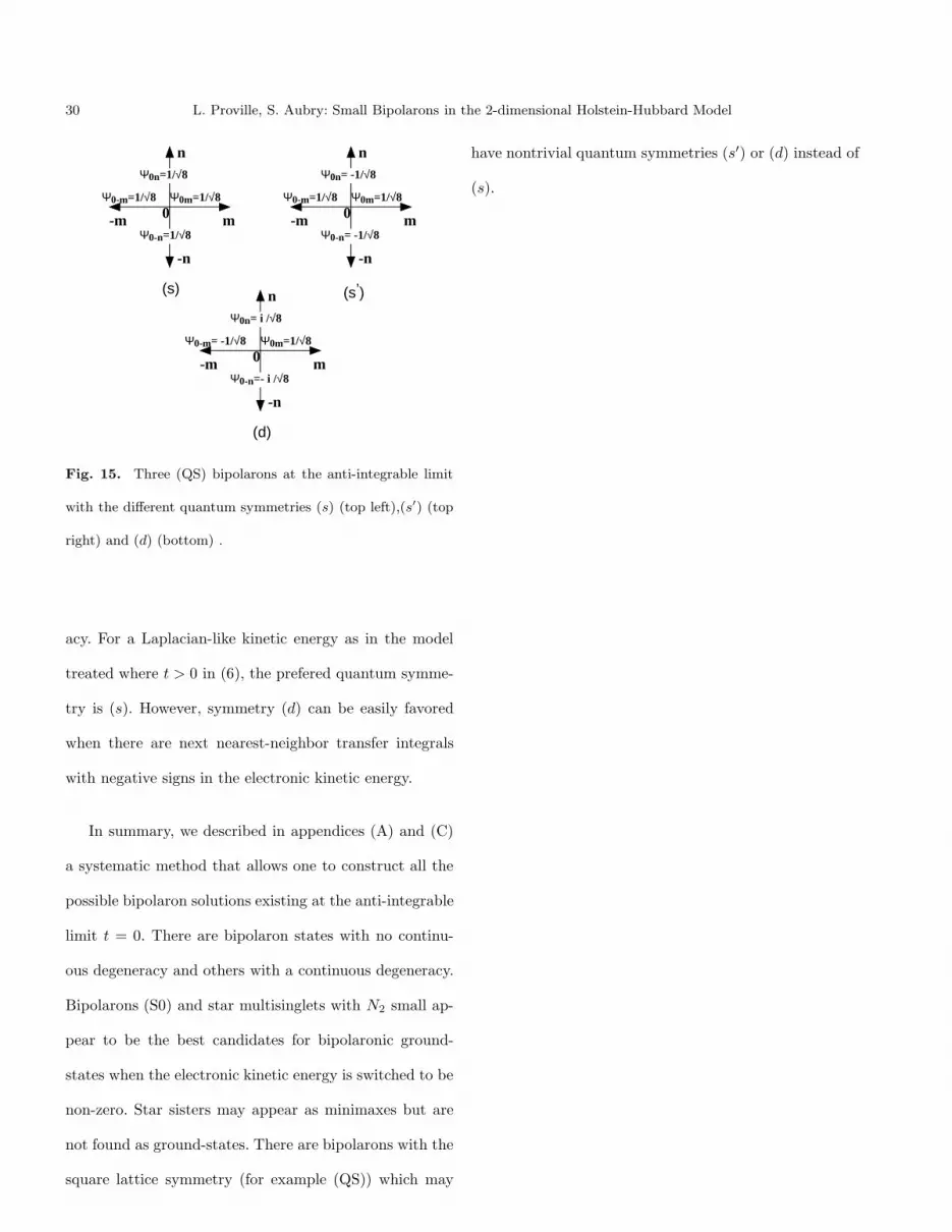
30 L. Proville, S. Aubry: Small Bipolarons in the 2-dimensional Holstein-Hubbard Model
Ψ0-m=1/√8
-m
Ψ0m=1/√8
Ψ0-n=1/√8
Ψ0n=1/√8
0 m
n
-n
(s)
Ψ0m=1/√8
Ψ0-n= -1/√8
Ψ0-m=1/√8
Ψ0n= -1/√8
0-m m
n
-n
(s’)
Ψ0m=1/√8
Ψ0-n=- i /√8
Ψ0-m= -1/√8
Ψ0n= i /√8
0-m m
n
-n
(d)
Fig. 15. Three (QS) bipolarons at the anti-integrable limit
with the different quantum symmetries (s) (top left),(s′) (top
right) and (d) (bottom) .
acy. For a Laplacian-like kinetic energy as in the model
treated where t > 0 in (6), the prefered quantum symme-
try is (s). However, symmetry (d) can be easily favored
when there are next nearest-neighbor transfer integrals
with negative signs in the electronic kinetic energy.
In summary, we described in appendices (A) and (C)
a systematic method that allows one to construct all the
possible bipolaron solutions existing at the anti-integrable
limit t = 0. There are bipolaron states with no continu-
ous degeneracy and others with a continuous degeneracy.
Bipolarons (S0) and star multisinglets with N2 small ap-
pear to be the best candidates for bipolaronic ground-
states when the electronic kinetic energy is switched to be
non-zero. Star sisters may appear as minimaxes but are
not found as ground-states. There are bipolarons with the
square lattice symmetry (for example (QS)) which may
have nontrivial quantum symmetries (s′) or (d) instead of
(s).


