Embed Size (px)
Citation preview
Computer Physics Communications 176 (2007) 539–549
www.elsevier.com/locate/cpc
Small scale localization in turbulent flows. A priori tests applied toa possible Large Eddy Simulation of compressible turbulent flows
Daniela Tordella a,∗, Michele Iovieno a, Silvano Massaglia b
a Politecnico di Torino, Dipartimento di Ingegneria Aeronautica e Spaziale, C.so Duca degli Abruzzi 24, 10129 Torino, Italyb Università degli Studi di Torino, Dipartimento di Fisica Generale, Via P. Giuria 1, 10125 Torino, Italy
Received 12 July 2006; accepted 16 December 2006
Available online 2 February 2007
Abstract
Amethod for the localization of small scales in turbulent velocity fields is proposed. The method is based on the definition of a function f of the
velocity and vorticity fields that reproduces a normalized form of the twisting-stretching term of the Helmholtz equation. By means of this method
the equations of motion can be selectively filtered in regions that are rich in small scale motions. The method is applied through a criterion built
on a statistical link between the function f and a local property of the turbulence that was derived from the analysis a homogeneous and isotropic
high Reynolds number (Reλ = 280) turbulence field. The localization criterion is independent of the subgrid scale model used in a possible Large
Eddy Simulation carried out after the small scale localization is obtained. This extends the typology of possible applications to the analysis of
experimental laboratory data. In case of compressible regimes, a second sensor that depends on the local pressure variation and divergence can be
associated to the previous one in order to determine the eventual emergence of shocks. The capture of shocks is made possible by suppressing the
subgrid terms where this second sensor indicates the presence of a shock.
A priori tests were carried out on the turbulent channel flow, Reλ = 180 and 590, to validate the localization procedure in a highly inhomoge-
neous flow configuration. A second set of a priori test was carried out on a turbulent time decaying jet which initiates its evolution at Mach 5 and
which reproduces a few hydrodynamical properties of high Reynolds number hypersonic jets which exist in the Universe.
2007 Elsevier B.V. All rights reserved.
PACS: 47.27.ep; 47.27.wg; 47.40.ki; 97.21.+a; 98.38.Fs
Keywords: Small scale localization; Astrophysical jets; Turbulence; Large eddy simulation
1. Introduction
The Large Eddy Simulation method is surely going to be
one of the most frequently used tools to predict the behavior of
turbulent flows in many different physical and engineering ap-
plications. Turbulent flows in nature are characterized by very
high Reynolds numbers. Consequently, any attempt to numeri-
cally solve the Navier–Stokes equations for such flows requires
a great number of scales to be resolved. At present, the largest
three-dimensional turbulence simulations have a resolution that
allows a ratio between the largest and the smallest scale of
about a thousand (see, for example, Kaneda and Ishihara 2006,
* Corresponding author.
E-mail address: [email protected] (D. Tordella).
isotropic turbulence in a box, 40963 grid points [1]). Thus, in
general, the large scales only of the flow can be accurately
simulated and a Large Eddy Simulation (LES) approach is con-
sidered appropriate. An instance of these occurrences is that of
astrophysical flows.
Astrophysical flows occur in very large sets of spatial scales
and velocities. Typical velocities for outflows from the Sun and
stars attain 200–400 km s−1 and form solar and stellar super-
sonic winds and jets; for outflows from collapsed objects, e.g.,
black holes, jets can reach the speed of light. Correspondingly,
the spatial scales range from hundreds of Astronomical Units,
for stellar outflows, up to hundreds of kiloparsecs for jets from
Active Galactic Nuclei (AGNs in the following). The resulting
Reynolds numbers exceed 1010–1013. Moreover, such flows are
hypersonic, with Mach numbers that attain values of up to ∼50
in Herbig–Haro jets and ∼100–1000 in jets from AGNs, with
0010-4655/$ – see front matter 2007 Elsevier B.V. All rights reserved.
doi:10.1016/j.cpc.2006.12.004
540 D. Tordella et al. / Computer Physics Communications 176 (2007) 539–549
the consequent formation of shocks. Three-dimensional DNS
of astrophysical flows undergoing shear-layer instabilities can,
nowadays and in a foreseeable future, capture just the behavior
that occurs at the largest scales (e.g., Bodo et al. [2], Micono et
al. [3]) but not the development of turbulent motions, which are
very likely induced by the instabilities.
In this context, there are two conflicting requirements: (1) to
capture discontinuities such as shock waves without the intro-
duction of spurious oscillations, which requires a relatively high
numerical dissipation, (2) the numerical algorithm should not
damp the resolved turbulent structures, which requires a low
numerical dissipation.
The problem of the reliable representation of small scales
in compressible turbulent flow simulations has often been over-
looked. It has often been assumed that numerical dissipation,
implicit in upwind shock capturing numerical schemes, could
simulate net energy transfer from larger to smaller scales. How-
ever, it has been shown, by Ducros et al. [4], that such an
approach is not compatible with LES modeling due to the an-
tithetic behavior of the high numerical viscosity which over-
whelms the subgrid scale term effects.
Our aim is the development of a general method that allows
the detection of small turbulence scales. In order to locate the
small scales, we propose the introduction of a criterion based
on the local structure of the vorticity field, in particular, on
its twisting and stretching intensity. In such a way, it would
be possible to selectively introduce a compressible sub-grid
scale model (for example, the Smagorinsky Model evaluated
by means of Favre-averaged quantities).
The criterion for the small scale localization, which is de-
scribed in Section 2, is based on the introduction of a local func-
tion f of the vorticity and velocity gradient and on Morkov-
in’s hypothesis (Morkovin [6]), which states that the essential
dynamics of supersonic turbulence follows the incompressible
pattern. Function f uses information from the stretching term
in the vorticity equation, which is responsible for the genera-
tion of smaller scales. The behavior of the function is observed
in a developed homogeneous and isotropic turbulence (HIT)
field, either fully resolved, by means of direct numerical sim-
ulation (DNS, Biferale et al. [7], Reλ = 280) or under-resolved,
by means of a sequence of filtering operations carried out using
different filter scales. The box filter has been used. A range of
f typical values for the homogeneous and isotropic turbulence
can be selected by means of a threshold tω and through the com-
putation of the probability density distribution that function f
is larger than a given threshold. The behavior of this thresh-
old tω is observed through a priori tests on high-resolution,
direct numerical simulation of incompressible homogeneous
and isotropic turbulence. A link with a statistical local property
of the turbulence is apparent. Values larger than a certain limit
value cannot be observed if the field is fully resolved. This ob-
servation has been exploited to build the localization criterion.
An earlier instance of localization procedure was the Se-
lective Structure-Function Model (SSF) developed in 1993 by
M. Lesieur and collaborators (see, e.g., Lesieur and Metais [8]).
In this study the idea was to switch off the turbulent viscos-
ity when the flow is not sufficiently three-dimensional. Based
on statistical data from Homogeneous Isotropic Turbulence, if
the angle between the vorticity—at a given grid point—and the
surrounding vorticity average exceeds a certain threshold (20
degrees), the eddy viscosity is settled. This threshold value re-
sults to depend on the resolution of the simulation, see again
Lesieur and Metais [8].
In the present paper we propose a function f that, besides
the twisting process, includes the stretching process. The dis-
cussion on the physical character and implications of function f
is in Section 2. This new localization criterion does not depend
on the simulation discretization. Before applying it to a priori
tests concerning the implementation of the Large Eddy Simu-
lation method to a highly inhomogeneous and anisotropic flow,
such as a supersonic turbulent jet, we present a further evidence
of the efficiency of the present localization criterion in the tur-
bulent channel flow. This flow, in fact, can be considered the
paradigm of inhomogeneous turbulent flows. The efficiency of
the use of this criterion in wall turbulence is obtained by com-
paring the distribution of the probability that f > tω in the DNS
of the turbulent channel flow at two values of Reynolds num-
ber (Reτ = 180 [9,10], Reτ = 590 [11]) and in few associated
filtered fields where the small scales where removed, see Sec-
tion 2.
The criterion was then applied to snapshots from a numeri-
cal simulation of the temporal decay of a hypersonic jet with
an initial Mach number of 5 (according to Bodo et al. [2],
Micono et al. [3], see also the review by Ferrari [13]), see Sec-
tion 3.2. This has made it possible to identify the presence of
small scales and then the region where it is opportune to fil-
ter the motion equations and insert a subgrid scale turbulence
model. In such a way the compressible momentum balance is
corrected by adding the contribution from the subgrid terms to
the turbulent stresses. This improves the general properties of
the jet—in particular, the spatial growth rate—obtaining values
which agree well with the central value of available experimen-
tal determinations (see, e.g., Brown and Roshko [15], Lu and
Lele [16], Slessor et al. [17], Smith and Dussage [18]). The
concluding remarks are given in Section 4.
2. Small scale localization criterion
The criterion for small scale localization is based on the in-
troduction of the function
(1)f (u,ω) =|ω · ∇u|
|ω|2,
where u is the velocity vector, and ω = curlu is the vorticity
vector.
Function f is a normalized form of the vortex-stretching
term in the Helmholtz equation. This term is responsible for
the generation of vortical three-dimensional small scales. It can
be observed that when the flow is three-dimensional and rich
in small scales f is necessarily different from zero. In gen-
eral, function f is zero in 2D vortical fields. When a mean
steady or unsteady shear flow is present, f is different from
zero. This also includes laminar flow configurations. To avoid
this problem, the dependence of f from the mean field must
D. Tordella et al. / Computer Physics Communications 176 (2007) 539–549 541
be removed by subtracting the mean field from the velocity and
vorticity fields. In such a way a function f ′ that only depend
on the fluctuation field can be introduced. Two formulation can
be proposed, the first to be used in a field obtained from direct
numerical simulation (DNS),
(2)f ′DNS(u,ω) =
|(ω − ω) · ∇(u − u)||ω − ω|2
,
where u, ω are the average of the velocity and vorticity that are
defined according to the space–time averaging introduced by
Monin and Yaglom [21, Section 3.1]
(3)g =∞
∫
−∞
∞∫
−∞
g(x − ξ , t − τ)ψ(ξ , τ )dξ dτ,
where g is a generic physical quantity and ψ(ξ ,τ ) is a weight-
ing function which satisfy the normalization condition
∞∫
−∞
∞∫
−∞
ψ(ξ ,τ )dξ dτ = 1.
The second formulation is to be used when dealing with filtered
fields coming from Large Eddy Simulations (LES)
(4)f ′LES
(
〈u〉, 〈ω〉)
=|(〈ω〉 − 〈ω〉) · ∇(〈u〉 − 〈u〉)|
|〈ω〉 − 〈ω〉|2,
where 〈·〉 indicated a filtered quantity. Again, quantities 〈u〉 and〈ω〉 are the mean of the filtered velocity and vorticity according
to definition (3).
The above remarks suggest the use of f ′ as a potential lo-
cal indicator of the presence of small scales in a 3D fluctuating
field where the stretching-twisting process is active. This can
made possible if a statistical link between the certainty of the
presence of small scales (as in high Reynolds number Homoge-
neous Isotropic Turbulence) and special values of the function
f ′ in such a flow can be found. To this end, a question can
be asked. Are there values of f ′ which can/cannot be found
in a highly developed turbulent field where the small scale are
surely present and, which, vice versa, cannot/can be found in a
coarser field as is the filtered field that is obtained from a LES?
In order to understand the behavior of f ′, with regards
to the local property of a fully developed turbulent flow,
f ′ is first observed in a fully resolved homogeneous and
isotropic incompressible turbulence, then in a few under-
resolved homogeneous-isotropic turbulences as well as in a
turbulent inhomogeneous field, as it is the channel flow. In these
fields, a typical range of f ′ values can be determined by consid-
ering a threshold tω and by computing the probability density
distribution that f ′ is larger than a chosen value both in the
resolved and under-resolved fields.
For this purpose, a priori tests have been carried out on a
DNS of a homogeneous and isotropic turbulence (in the fol-
lowing called HIT, 10243 grid, Reλ = 280, see Biferale et
al. [7]) and on four box filtered fields with resolutions of
643,1283,2563 and 5123 deduced from this DNS. The 10243
turbulence is here considered a resolved fully developed tur-
bulent field and is taken as a reference. The function f ′ is
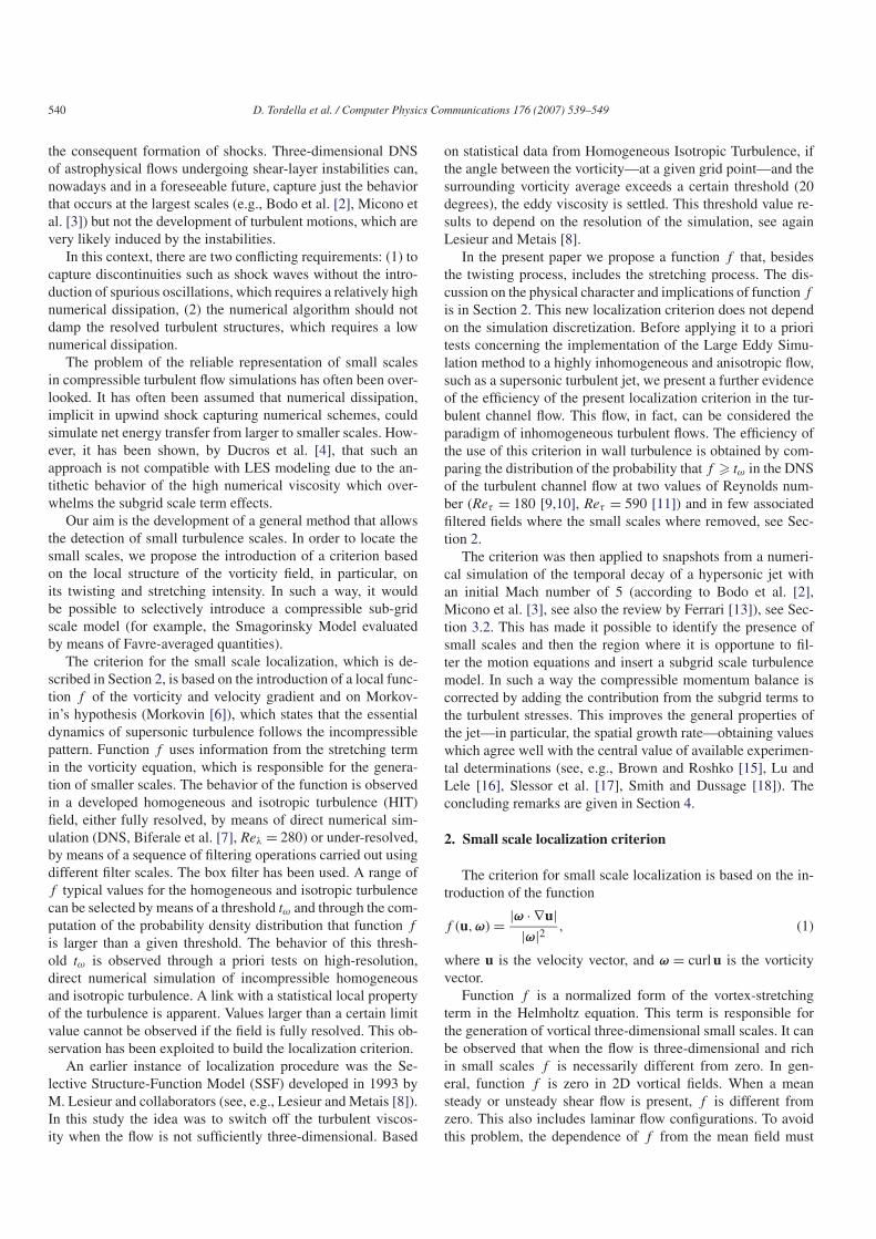
Fig. 1. Distribution of the probability of f ′ for different resolutions of incom-
pressible homogeneous and isotropic turbulence (sensor f ′DNS for the resolu-
tion 10243 , sensor f ′LES for the filtered fields).
computed for all the fields. As previously mentioned, the range
of the possible f ′ values in a resolved HIT and in an under-
resolved HIT can be obtained by considering a threshold tωand by computing the probability density distribution that f ′ islarger than the given value. In Fig. 1, it can be noticed that there
is an almost zero probability of having f ′ > tω ≈ 0.5 in the re-
solved turbulence. This value can be regarded as the maximum
stretching which a turbulent flow with a fine grain can yield.
On the contrary, in the unresolved cases, larger values are pos-
sible, with a probability that is in [0,0.2]. Thus, in theory, if
in a simulation of a fully developed turbulent flow, f ′ assumes
values larger than 0.5, the turbulent field should be considered
under-resolved and should benefit from the local activation of
the Large Eddy Simulation method (LES) by inserting a sub-
grid scale term in the motion equation. In this way, we consider
regions where f ′ is higher than tω as under-resolved regions
where there should be scales that are smaller than the local filter
scale and where the activation of a LES procedure is opportune.
It should be noticed that the value of tω, which gives an ex-
actly zero p(f ′ > tω) is not numerically well determinable. It is
opportune to fix a value that corresponds to a sufficiently small
finite probability. We have considered that a threshold, where
f ′ values with a probability of about 2 out of 100 can be al-
lowed, can be reasonable. From the 10243 grid curve in Fig. 1,
this yields tω ∼ 0.40 (that is, p(f ′ > tω) ∼ 0.02).
To verify the reliability of this proposal in a highly inho-
mogeneous turbulent field, we considered the direct numerical
simulation of a turbulent channel flow at Reτ = 180 with a grid
resolution of (Nx,Ny,Nz) = (96,128,64) [9] and its filtered
counterpart with a resolution of (Nx,Ny,Nz) = (48,65,32)
points in the streamwise, normal and spanwise directions, re-
spectively, as well as the direct numerical simulations of a
turbulent channel flow at Reτ = 590 with a grid resolution
of (Nx,Ny,Nz) = (384,257,384) [11] and its two filtered
counterparts with resolution (Nx,Ny,Nz) = (96,129,96) and
(Nx,Ny,Nz) = (192,185,192). We computed f ′DNS, relation
(2), in the DNS fields and f ′LES, relation (4), in the filtered
fields. Then, we compared the probability distributions that
542 D. Tordella et al. / Computer Physics Communications 176 (2007) 539–549
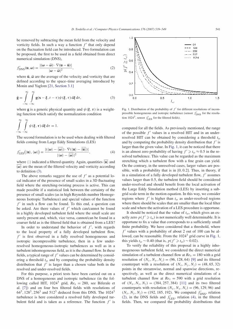
Fig. 2. Distribution of probability that p(f ′ > 0.4) along the channel
width. The filter is uniform in streamwise (x) and spanwise (z) directions,
while it varies as an hyperbolic tangent in the wall normal direction y.
The filter widths are: for the resolution 192 × 185 × 192: δx/Lx = 0.01,
δz/Lz = 0.01, δy (0)/h = 0.012; for the resolution 96 × 129 × 96:
δx/Lx = 0.02, δz/Lz = 0.02, δy (0)/h = 0.025; for the resolution 48×65×32:
δx/Lx = 0.04, δz/Lz = 0.06, δy (0)/h = 0.05. The domain of all simula-
tions is Lx = 2πh, Lz = πh, where h is the channel halfwidth. Probabilities
at Reτ = 590 are computed using the instantaneous field available online at
http://davinci.tam.uiuc.edu/data/moser/chandata (see [11]).
function f > tω across the channel in the highly resolved DNS
fields and in the filtered fields. Fig. 2 shows these distributions.
Once again it can be seen that the field which contains the
smallest scales relevant to its proper Reynolds number shows
a very low probability. In fact, in Fig. 2 one can see that the
curve which represents the DNS field by Moser et al. [11]
shows a probability as low as 0.03, i.e. of the order of the
probability p(f ′ > 0.4) ∼ 0.02 which is observed in the 10243
HIT. This small difference can be considered due to the nu-
merical uncertainty, but also to the fact that the curve that
represents this DNS field is not the result of a statistical av-
erage because one temporal instant only is available for this
data base (see http://davinci.tam.uiuc.edu/data/moser/chandata,
[11]). The DNS at Reτ = 180 shows a probability of about
0.06. This DNS has statistics in excellent agreement with other
analogous DNS and with laboratory data, see also [10], but, ac-
cording with the present criterion of subgrid scale localization,
is not perfectly resolved. In fact, the value 0.06, though small,
is definitely higher than the uncertainty threshold that we pro-
pose, that is a too a high value to be interpreted as exclusively
due to the computational uncertainty. A posteriori, we think that
the explanation is a non-sufficient resolution in the spanwise
direction where we put 64 points only. Fig. 2 also shows that
the filtered fields always have high values of the probability
p(f ′ > tω). The lower the resolution the higher the probabil-
ity, a fact that is in full agreement with what is observed in the
Homogeneous Isotropic Turbulence, see Fig. 1, and which sup-
ports the proposed small scale localization criterion.
Underlying the present small scale localization criterion, is
the hypothesis that the compressibility effects do not have much
influence on the turbulence dynamics, apart from varying the
local fluid properties (Morkovin [6], Duros et al. [4]).
3. Application to the time evolution of a highly
compressible turbulent jet
3.1. Description of the test flows
Astrophysical jets are highly collimated supersonic flows
that emerge from objects, such as neutron stars, Young Stel-
lar Objects (YSOs) or the supermassive black holes that are
thought to power the galactic nuclei. The mass accretion–
ejection phenomenon is usually mediated by an accretion disk.
According to this scheme, jets are accelerated via magneto-
centrifugal processes in the vicinities of the accreting object.
As previously mentioned, jets are usually hypersonic and, in
many instances, relativistic and are subject to shear-layer (or
Kelvin–Helmholtz) instabilities (see Ferrari [13] for a review).
We have studied numerically, and in Cartesian geometry, the
temporal evolution of a 3D jet subject to periodicity conditions
along the longitudinal direction. The flow is governed by the
ideal fluid equations for mass, momentum, and energy conser-
vation, in the non-relativistic limit (as appropriate for the case
of Herbig–Haro jets)
(5)∂ρ
∂t+ ∇ · (ρv) = 0,
(6)ρ
[
∂v
∂t+ (v · ∇)v
]
= −∇p,
(7)∂p
∂t+ (v · ∇)p − Γ
p
ρ
[
∂ρ
∂t+ (v · ∇)ρ
]
= 0,
where the fluid variables p, ρ and v are, as customary, the pres-
sure, density, and velocity, respectively; Γ (= 5/3) is the ratio
of the specific heats.
The initial flow structure is a cylindrical jet in the 3D do-
main {(0,D) × (−R,R) × (−R,R)}, described by a Cartesian
coordinate system (x, y, z). The initial jet velocity is along the
x-direction; its symmetry axis is defined by (y = 0, z = 0).
The initial jet velocity, at t = 0, is Vx(y, z) = V0 within the
jet, i.e. for (y, z) 6 a, where a is the initial jet radius, and
Vx(y, z) = 0 elsewhere. The initial particle density is set to
ρ(y, z) = ρ0 within the jet and ρ(y, z) = νρ0 outside, with ν
the initial density ratio of the external medium to jet proper. Fi-
nally, we assume that the jet is initially in pressure equilibrium
with its surroundings; for this reason, we assume an initially
uniform pressure distribution p0.
In the following, we will express lengths in units of the initial
jet radius a, times in units of the sound crossing time of the
radius a/c0 (with c0 =√
Γp0/ρ0), velocities in units of c0 (thus
coinciding with the initial Mach number), densities in units of
ρ0 and pressures in units of p0.
This initial configuration is then perturbed at t = 0. The par-
ticular functional form of this perturbation is such as to excite a
wide range of modes. Thus, we impose a superposition of lon-
gitudinally periodic transverse velocity disturbances, using the
functional forms
(8)vy(x, y, z) = Vy,0
n0∑
n=1
sin(nk0x + φn),
D. Tordella et al. / Computer Physics Communications 176 (2007) 539–549 543
(9)vz(x, y, z) = Vy,0
n0∑
n=1
cos(nk0x + φn),
where Vy,0 = 0.01V0 and {φn} are the phase shifts of the var-
ious Fourier components. These perturbations are therefore a
superposition of a fundamental mode, plus a number of its har-
monics. This form also allows us to choose n0 harmonics. In
the following, we have used the value n0 = 8; this value is suf-
ficiently small for the shortest wavelength mode excited to still
be accurately followed in time (i.e. to be adequately resolved)
by our calculations.
The wavelength of the fundamental mode is set equal to
the length of the computational domain; thus, k0 = 2π/D,
therefore if we set k0 = 0.2, D = 10π . The shortest perturba-
tion wavelength, 2πn0/k0, is fixed by the maximum value of
n = n0, which—as already mentioned—is set at n0 = 8. It is
essential to note that the fundamental mode (of wavelength D)
does not necessarily coincide with the most unstable mode; the
wavelength of the most unstable mode depends on the actual
values of the parameters that characterize the initial state of the
jet.
We cover our integration domain (0 6 x 6 D, −R 6 y 6 R,
−R 6 z 6 R) by a 1283 or 2563 grid, with R = 6. We have
adopted free boundary conditions at the outer y and z bound-
aries (y = ±R, z = ±R), that is, the gradient of each variable is
set to zero at these boundaries, while periodic boundary condi-
tions have been imposed in the longitudinal direction x. The
main control parameters of this problem are the initial flow
Mach number M ≡ V0/c0 and the density ratio ν.
The hydrodynamic equations (4), (5) and (6), supplemented
with the previously described initial and boundary conditions,
were solved using the PLUTO code (described in [14] and
in http://plutocode.to.astro.it). This Godunov-type code sup-
plies a series of high-resolution shock-capturing schemes that
are particularly suitable for the present application. In order
to discretize the Euler equations, we chose a version of the
Piecewise-Parabolic-Method (PPM) [19], which is third-order
accurate in space and second-order in time.
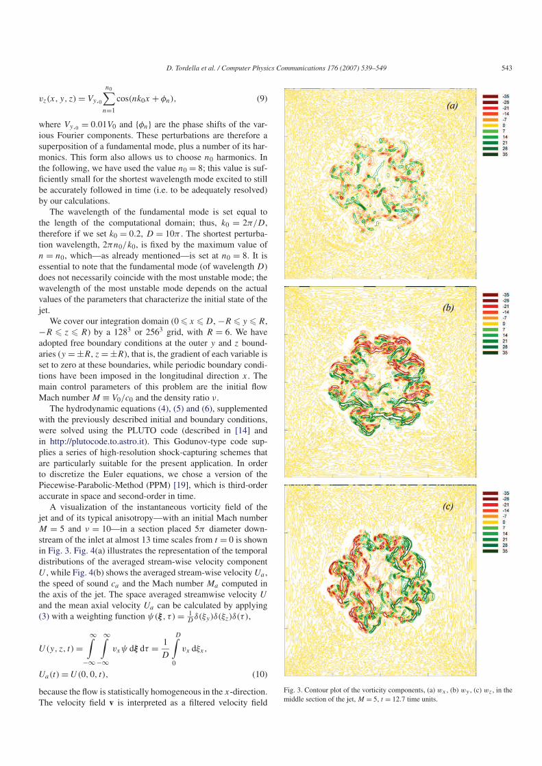
A visualization of the instantaneous vorticity field of the
jet and of its typical anisotropy—with an initial Mach number
M = 5 and ν = 10—in a section placed 5π diameter down-
stream of the inlet at almost 13 time scales from t = 0 is shown
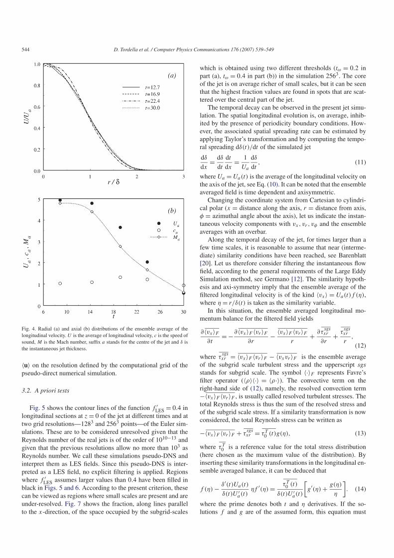
in Fig. 3. Fig. 4(a) illustrates the representation of the temporal
distributions of the averaged stream-wise velocity component
U , while Fig. 4(b) shows the averaged stream-wise velocity Ua ,
the speed of sound ca and the Mach number Ma computed in
the axis of the jet. The space averaged streamwise velocity U
and the mean axial velocity Ua can be calculated by applying
(3) with a weighting function ψ(ξ , τ ) = 1D
δ(ξy)δ(ξz)δ(τ ),
U(y, z, t) =∞
∫
−∞
∞∫
−∞
vxψ dξ dτ =1
D
D∫
0
vx dξx,
(10)Ua(t) = U(0,0, t),
because the flow is statistically homogeneous in the x-direction.
The velocity field v is interpreted as a filtered velocity field
Fig. 3. Contour plot of the vorticity components, (a) wx , (b) wy , (c) wz , in the
middle section of the jet, M = 5, t = 12.7 time units.
544 D. Tordella et al. / Computer Physics Communications 176 (2007) 539–549
Fig. 4. Radial (a) and axial (b) distributions of the ensemble average of the
longitudinal velocity. U is the average of longitudinal velocity, c is the speed of
sound, M is the Mach number, suffix a stands for the centre of the jet and δ is
the instantaneous jet thickness.
〈u〉 on the resolution defined by the computational grid of the
pseudo-direct numerical simulation.
3.2. A priori tests
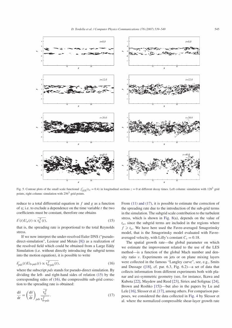
Fig. 5 shows the contour lines of the function f ′LES = 0.4 in
longitudinal sections at z = 0 of the jet at different times and at
two grid resolutions—1283 and 2563 points—of the Euler sim-
ulations. These are to be considered unresolved given that the
Reynolds number of the real jets is of the order of 1010−13 and
given that the previous resolutions allow no more than 103 as
Reynolds number. We call these simulations pseudo-DNS and
interpret them as LES fields. Since this pseudo-DNS is inter-
preted as a LES field, no explicit filtering is applied. Regions
where f ′LES assumes larger values than 0.4 have been filled in
black in Figs. 5 and 6. According to the present criterion, these
can be viewed as regions where small scales are present and are
under-resolved. Fig. 7 shows the fraction, along lines parallel
to the x-direction, of the space occupied by the subgrid-scales
which is obtained using two different thresholds (tω = 0.2 in
part (a), tω = 0.4 in part (b)) in the simulation 2563. The core
of the jet is on average richer of small scales, but it can be seen
that the highest fraction values are found in spots that are scat-
tered over the central part of the jet.
The temporal decay can be observed in the present jet simu-
lation. The spatial longitudinal evolution is, on average, inhib-
ited by the presence of periodicity boundary conditions. How-
ever, the associated spatial spreading rate can be estimated by
applying Taylor’s transformation and by computing the tempo-
ral spreading dδ(t)/dt of the simulated jet
(11)dδ
dx=
dδ
dt
dt
dx=
1
Ua
dδ
dt,
where Ua = Ua(t) is the average of the longitudinal velocity on
the axis of the jet, see Eq. (10). It can be noted that the ensemble
averaged field is time dependent and axisymmetric.
Changing the coordinate system from Cartesian to cylindri-
cal polar (x = distance along the axis, r = distance from axis,
φ = azimuthal angle about the axis), let us indicate the instan-
taneous velocity components with vx, vr , vφ and the ensemble
averages with an overbar.
Along the temporal decay of the jet, for times larger than a
few time scales, it is reasonable to assume that near (interme-
diate) similarity conditions have been reached, see Barenblatt
[20]. Let us therefore consider filtering the instantaneous flow
field, according to the general requirements of the Large Eddy
Simulation method, see Germano [12]. The similarity hypoth-
esis and axi-symmetry imply that the ensemble average of the
filtered longitudinal velocity is of the kind 〈vx〉 = Ua(t)f (η),
where η = r/δ(t) is taken as the similarity variable.
In this situation, the ensemble averaged longitudinal mo-
mentum balance for the filtered field yields
(12)
∂〈vx〉F∂t
= −∂〈vx〉F 〈vr〉F
∂r−
〈vx〉F 〈vr 〉Fr
+∂τ
sgsxr
∂r+
τsgsxr
r,
where τsgsxr = 〈vx〉F 〈vr〉F − 〈vxvr〉F is the ensemble average
of the subgrid scale turbulent stress and the upperscript sgs
stands for subgrid scale. The symbol 〈·〉F represents Favre’s
filter operator (〈ρ〉〈·〉 = 〈ρ·〉). The convective term on the
right-hand side of (12), namely, the resolved convection term
−〈vx〉F 〈vr 〉F , is usually called resolved turbulent stresses. The
total Reynolds stress is thus the sum of the resolved stress and
of the subgrid scale stress. If a similarity transformation is now
considered, the total Reynolds stress can be written as
(13)−〈vx〉F 〈vr 〉F + τsgsxr = τT
0 (t)g(η),
where τT0 is a reference value for the total stress distribution
(here chosen as the maximum value of the distribution). By
inserting these similarity transformations in the longitudinal en-
semble averaged balance, it can be deduced that
(14)f (η) −δ′(t)Ua(t)
δ(t)U ′a(t)
ηf ′(η) =τT0 (t)
δ(t)U ′a(t)
[
g′(η) +g(η)
η
]
.
where the prime denotes both t and η derivatives. If the so-
lutions f and g are of the assumed form, this equation must
D. Tordella et al. / Computer Physics Communications 176 (2007) 539–549 545
Fig. 5. Contour plots of the small scale functional f ′LES(tω = 0.4) in longitudinal sections z = 0 at different decay times. Left column: simulation with 1283 grid
points, right column: simulation with 2563 grid points.
reduce to a total differential equation in f and g as a function
of η; i.e. to exclude a dependence on the time variable t the two
coefficients must be constant, therefore one obtains
(15)δ′(t)Ua(t) ∝ τT0 (t),
that is, the spreading rate is proportional to the total Reynolds
stress.
If we now interpret the under-resolved Euler DNS (“pseudo-
direct-simulation”, Lesieur and Metais [8]) as a realization of
the resolved field which could be obtained from a Large Eddy
Simulation (i.e. without directly introducing the subgrid terms
into the motion equation), it is possible to write
(16)δ′pds(t)U0-pds(t) ∝ τT
0-pds(t),
where the subscript pds stands for pseudo-direct simulation. By
dividing the left- and right-hand sides of relation (15) by the
corresponding sides of (16), the compressible sub-grid correc-
tion to the spreading rate is obtained:
(17)dδ
dt=
(
dδ
dt
)
pds
τT0
τT0-pds
.
From (11) and (17), it is possible to estimate the correction of
the spreading rate due to the introduction of the sub-grid terms
in the simulation. The subgrid scale contribution to the turbulent
stress, which is shown in Fig. 8(a), depends on the value of
tω, since the subgrid terms are included in the regions where
f > tω. We have here used the Favre-averaged Smagorinsky
model, that is the Smagorinsky model evaluated with Favre-
averaged velocity, with Lilly’s constant Cs = 0.18.
The spatial growth rate—the global parameter on which
we estimate the improvement related to the use of the LES
method—is a function of the global Mach number and den-
sity ratio ν. Experiments on jets or on plane mixing layers
were collected in the famous “Langley curve”, see, e.g., Smits
and Dussage ([18], cf. par. 6.3, Fig. 6.2)—a set of data that
collects information from different experiments both with pla-
nar and axi-symmetric geometry (see, for instance, Ikawa and
Kubota [22], Maydew and Reed [23], Siriex and Solignac [24],
Brown and Roshko [15])—but also in the papers by Lu and
Lele [16], Slessor et al. [17], among others. For comparison pur-
poses, we considered the data collected in Fig. 4 by Slessor et
al. where the normalized compressible shear-layer growth rate
546 D. Tordella et al. / Computer Physics Communications 176 (2007) 539–549
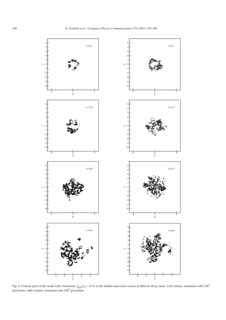
Fig. 6. Contour plots of the small scales functional f ′LES(tω = 0.4) in the middle transversal section at different decay times. Left column: simulation with 1283
grid points, right column: simulation with 2563 grid points.
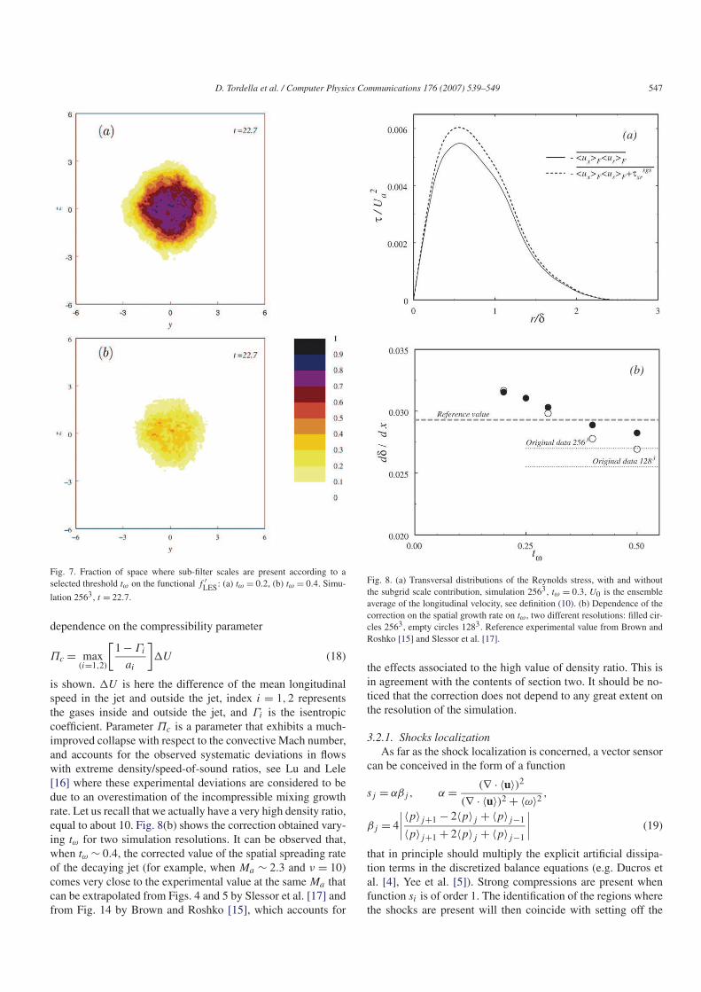
D. Tordella et al. / Computer Physics Communications 176 (2007) 539–549 547
Fig. 7. Fraction of space where sub-filter scales are present according to a
selected threshold tω on the functional f ′LES: (a) tω = 0.2, (b) tω = 0.4. Simu-
lation 2563 , t = 22.7.
dependence on the compressibility parameter
(18)Πc = max(i=1,2)
[
1− Γi
ai
]
1U
is shown. 1U is here the difference of the mean longitudinal
speed in the jet and outside the jet, index i = 1,2 represents
the gases inside and outside the jet, and Γi is the isentropic
coefficient. Parameter Πc is a parameter that exhibits a much-
improved collapse with respect to the convective Mach number,
and accounts for the observed systematic deviations in flows
with extreme density/speed-of-sound ratios, see Lu and Lele
[16] where these experimental deviations are considered to be
due to an overestimation of the incompressible mixing growth
rate. Let us recall that we actually have a very high density ratio,
equal to about 10. Fig. 8(b) shows the correction obtained vary-
ing tω for two simulation resolutions. It can be observed that,
when tω ∼ 0.4, the corrected value of the spatial spreading rate
of the decaying jet (for example, when Ma ∼ 2.3 and ν = 10)
comes very close to the experimental value at the same Ma that
can be extrapolated from Figs. 4 and 5 by Slessor et al. [17] and
from Fig. 14 by Brown and Roshko [15], which accounts for
Fig. 8. (a) Transversal distributions of the Reynolds stress, with and without
the subgrid scale contribution, simulation 2563 , tω = 0.3, U0 is the ensemble
average of the longitudinal velocity, see definition (10). (b) Dependence of the
correction on the spatial growth rate on tω , two different resolutions: filled cir-
cles 2563 , empty circles 1283 . Reference experimental value from Brown and
Roshko [15] and Slessor et al. [17].
the effects associated to the high value of density ratio. This is
in agreement with the contents of section two. It should be no-
ticed that the correction does not depend to any great extent on
the resolution of the simulation.
3.2.1. Shocks localization
As far as the shock localization is concerned, a vector sensor
can be conceived in the form of a function
sj = αβj , α =(∇ · 〈u〉)2
(∇ · 〈u〉)2 + 〈ω〉2,
(19)βj = 4
∣
∣
∣
∣
〈p〉j+1 − 2〈p〉j + 〈p〉j−1
〈p〉j+1 + 2〈p〉j + 〈p〉j−1
∣
∣
∣
∣
that in principle should multiply the explicit artificial dissipa-
tion terms in the discretized balance equations (e.g. Ducros et
al. [4], Yee et al. [5]). Strong compressions are present when
function si is of order 1. The identification of the regions where
the shocks are present will then coincide with setting off the
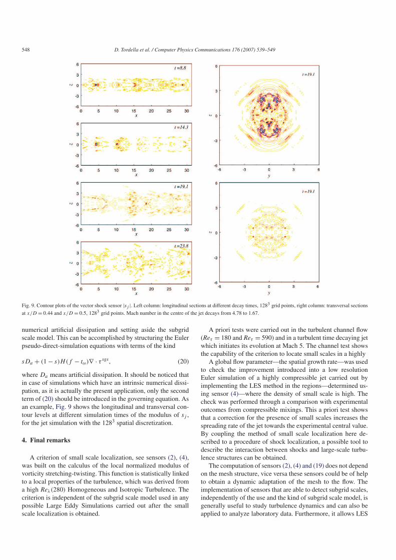
548 D. Tordella et al. / Computer Physics Communications 176 (2007) 539–549
Fig. 9. Contour plots of the vector shock sensor |sj |. Left column: longitudinal sections at different decay times, 1283 grid points, right column: transversal sections
at x/D = 0.44 and x/D = 0.5, 1283 grid points. Mach number in the centre of the jet decays from 4.78 to 1.67.
numerical artificial dissipation and setting aside the subgrid
scale model. This can be accomplished by structuring the Euler
pseudo-direct-simulation equations with terms of the kind
(20)sDa + (1 − s)H(f − tω)∇ · τ sgs,
where Da means artificial dissipation. It should be noticed that
in case of simulations which have an intrinsic numerical dissi-
pation, as it is actually the present application, only the second
term of (20) should be introduced in the governing equation. As
an example, Fig. 9 shows the longitudinal and transversal con-
tour levels at different simulation times of the modulus of sj ,
for the jet simulation with the 1283 spatial discretization.
4. Final remarks
A criterion of small scale localization, see sensors (2), (4),
was built on the calculus of the local normalized modulus of
vorticity stretching-twisting. This function is statistically linked
to a local properties of the turbulence, which was derived from
a high Reλ(280) Homogeneous and Isotropic Turbulence. The
criterion is independent of the subgrid scale model used in any
possible Large Eddy Simulations carried out after the small
scale localization is obtained.
A priori tests were carried out in the turbulent channel flow
(Reτ = 180 and Reτ = 590) and in a turbulent time decaying jet
which initiates its evolution at Mach 5. The channel test shows
the capability of the criterion to locate small scales in a highly
A global flow parameter—the spatial growth rate—was used
to check the improvement introduced into a low resolution
Euler simulation of a highly compressible jet carried out by
implementing the LES method in the regions—determined us-
ing sensor (4)—where the density of small scale is high. The
check was performed through a comparison with experimental
outcomes from compressible mixings. This a priori test shows
that a correction for the presence of small scales increases the
spreading rate of the jet towards the experimental central value.
By coupling the method of small scale localization here de-
scribed to a procedure of shock localization, a possible tool to
describe the interaction between shocks and large-scale turbu-
lence structures can be obtained.
The computation of sensors (2), (4) and (19) does not depend
on the mesh structure, vice versa these sensors could be of help
to obtain a dynamic adaptation of the mesh to the flow. The
implementation of sensors that are able to detect subgrid scales,
independently of the use and the kind of subgrid scale model, is
generally useful to study turbulence dynamics and can also be
applied to analyze laboratory data. Furthermore, it allows LES
D. Tordella et al. / Computer Physics Communications 176 (2007) 539–549 549
of complex flows to be obtained without a priori assumptions of
the flow structure. The local character of such functions should
allow easy parallelization.
Acknowledgements
The numerical calculations were performed at CINECA,
in Bologna, Italy, thanks to the support of INAF (Istituto
Nazionale di Astrofisica). We would like to thank Andrea
Mignone for his assistance in carrying out the numerical simu-
lations.
References
[1] Y. Kaneda, T. Ishihara, High-resolution direct numerical simulation of tur-
bulence, Journal of Turbulence 7 (20) (2006) 1–17.
[2] G. Bodo, P. Rossi, S. Massaglia, Three-dimensional simulations of jets,
Astron. Astrophys. 333 (1998) 1117–1129.
[3] M. Micono, G. Bodo, S. Massaglia, P. Rossi, A. Ferrari, R. Rosner,
Kelvin–Helmholtz instabilities in three-dimensional radiative jets, Astron.
Astrophys. 360 (2000) 795–808.
[4] F. Ducros, V. Ferrand, F. Nicoud, C. Weber, D. Darracq, C. Gacherieu,
T. Poinsot, Large-eddy simulation of the shock-turbulence interaction,
J. Comp. Phys. 152 (1999) 517–549.
[5] H.C. Yee, N.D. Sandham, M.J. Djomehri, Low-dissipative high-order
shock-capturing methods using characteristic-based filters, J. Comp.
Phys. 150 (1999) 199–238.
[6] M.V. Morkovin, Effects of compressibility on turbulent flows, in: A. Favre
(Ed.), Mècanique de la turbulence, 1961, p. 367.
[7] L. Biferale, G. Boffetta, A. Celani, A. Lanotte, F. Toschi, Particle trap-
ping in three-dimensional fully developed turbulence, Phys. Fluids 17 (2)
(2005), 021701/1–4.
[8] M. Lesieur, O. Metais, New trends in large eddy simulations of turbulent
flows, Annu. Rev. Fluid Mech. 28 (1996) 45–83.
[9] M. Iovieno, G. Passoni, D. Tordella, A new large-eddy simulation near-
wall treatment, Phys. Fluids 16 (11) (2004) 3935–3944.
[10] M. Iovieno, G. Passoni, D. Tordella, Vorticity fluctuation in the LES of the
channel flow through new wall condition and the noncommutation error
procedure, in: H.I. Andersson, P.A. Krogstad (Eds.), Advances in Turbu-
lence, vol. 10, CIMNE, Barcelona, 2004, pp. 245–248.
[11] R.D. Moser, J. Kim, N.N. Mansour, Direct numerical simulation of turbu-
lent channel flow up to Reτ = 590, Phys. Fluids 11 (4) (1999) 943–945.
[12] M. Germano, Turbulence, the filtering approach, J. Fluid Mech. 236
(1992) 325–336.
[13] A. Ferrari, Modeling extragalactic jets, Annu. Rev. Astron. Astrophys. 36
(1998) 539–598.
[14] A. Mignone, G. Bodo, S. Massaglia, T. Matsakos, O. Tesileanu, C. Zanni,
A. Ferrari, PLUTO: a numerical code for computational astrophysics, As-
trophys. J. (2006).
[15] G.L. Brown, A. Roshko, On density effects and large structure in turbulent
mixing layers, J. Fluid Mech. 64 (1974) 775–816.
[16] G. Lu, S.K. Lele, On the density ratio effect on the growth-rate of a com-
pressible mixing layer, Phys. Fluids 6 (2) (1994) 1073–1075.
[17] M.D. Slessor, M. Zhuang, P.E. Dimotakis, Turbulent shear-layer mixing:
growth-rate compressibility scaling, J. Fluid Mech. 414 (2000) 35–45.
[18] J. Smits, J.P. Dussage, Turbulent Shear Layers in Supersonic Flow, AIP
Press, Woodbury, New York, 1996.
[19] P. Colella, P.R. Woodward, The piecewise parabolic method (PPM) for
gas-dynamical simulations, J. Comp. Phys. 54 (1) (1984) 174–201.
[20] G.I. Barenblatt, Scaling, Self-Similarity, and Intermediate Asymptotics,
Cambridge University Press, 1996, cf. Preface, p. xiii.
[21] A.S. Monin, A.M. Yaglom, Statistical Fluid Mechanics, vol. 1, MIT Press,
Cambridge, 1979.
[22] H. Ikawa, T. Kubota, Investigation of supersonic turbulent mixing layer
with zero pressure gradient, AIAA J. 13 (1975) 566–572.
[23] R.C. Maydew, J.F. Reed, Turbulent mixing of compressible free jets,
AIAA J. 1 (1963) 1443.
[24] M. Sirieix, J.L. Solignac, Contribution à l’étude experimentale de la
couche de melange turbulent isobare d’un ecoulment supersonique, in:
Separated Flows, AGARD CP4, 1966.


