Embed Size (px)
Citation preview

ADDIS ABABA UNIVERSITY
ADDIS ABABA INSTITUTE OF TECHNOLOGY
DEPARTMENT OF ELECTRICAL AND COMPUTER ENGINEERING
ASSESSMENT OF RESOURCE POTENTIAL AND MODELING OF
STANDALONE PV/WIND HYBRID SYSTEM FOR RURAL
ELECTRFICATION, CASE STUDY AXUM DISTRICT
A THESIS SUBMITTED TO THE ADDIS ABABA INSTITUTE OF
TECHNOLOGY, SCHOOL OF GRADUATE STUDIES OF ADDIS
ABABA UNIVERSITY
IN PARTIAL FULFILLMENT OF THE REQUIRMENT FOR THE
DEGREE OF
MASTER OF SCIENCE IN ELECTRICAL AND COMPUTER
ENGINEERING
BY
SOLOMON KIROS
ADVISOR
DR. GETACHEW BEKELE
JULY 2014
ADDIS ABABA UNIVERSITY
SCHOOL OF GRADUATE STUDIES
ASSESSMENT OF RESOURCE POTENTIAL AND MODELING OF
STANDALONE PV/WIND HYBRID SYSTEM FOR RURAL
ELECTRFICATION, CASE STUDY AXUM DISTRICT
ADDIS ABABA UNIVERSITY
ADDIS ABABA INSTITUTE OF TECHNOLOGY
DEPARTMENT OF ELECTRICAL AND COMPUTER ENGINEERING
By
Solomon Kiros
Advisor
Dr. Getachew Bekele
July 2014
ADDIS ABABA UNIVERSITY
SCHOOL OF GRADUATE STUDIES
ASSESSMENT OF RESOURCE POTENTIAL AND MODELING OF
STANDALONE PV/WIND HYBRID SYSTEM FOR RURAL
ELECTRFICATION, CASE STUDY AXUM DISTRICT
By
Solomon Kiros
Approved by Board of Examiners
Dr. Getachew Bekele ____________ ____________
Advisor Signature Date
Prof. Singh ____________ ____________
External Examiner Signature Date
Dr. Solomon Abebe ____________ ___________
Internal Examiner Signature Date
____________ ____________
Chairman Signature Date

i
DECLARATION
I hereby declare that the work which is being presented in this thesis entitles “ASSESSMENT
OF RESOURCE POTENTIAL AND MODELING OF STAND ALONE PV/WIND
HYBRID SYSTEM FOR RURAL ELECTRFICATION, CASE STUDY IN AXUM
DISTRICT” is original work of my own, has not been presented for a degree in any other
university and that all sources of material used for the thesis have been duly acknowledged.
--------------------------------------------- --------------------------
Solomon Kiros Date
(Candidate)
This is to certify that the above declaration made by the candidate is correct to the best of my
knowledge.
--------------------------------------------- --------------------------
Dr. Getachew Bekele Date
(Thesis Advisor)

ii
Acknowledgment
Most of all I would like to thank the almighty God because this work was impossible without his
blessings and wills. At the beginning of my MSc I was not even confident to define what a
research mean, but now due to the help of one person I am able to understand it. That person is
Dr. Getachew Bekele who was my advisor in this thesis. He gave me valuable advices throughout
the research. So I want to thank him for his continuous follow up and encouragement to the
successful accomplishment of my work.
I am also very much grateful to my wife Genet Kefyalew for her uninterrupted support and
encouragement as well as her brilliant approach in handling all household matters without my
help. She sacrificed a lot by giving priority for the successful accomplishment of my thesis work.
I also wish to express my thanks to Weldie not only for his help in collecting the data required for
the analysis part of my work but also for his constructive comments he gave me by reviewing the
research. Finally I want to thank Anbesa, Fishatsion kebede, Afewerki leake for their commitment
in arranging transportation and Tsegay mebrahtu for driving me to the selected village.
iii
Abstract
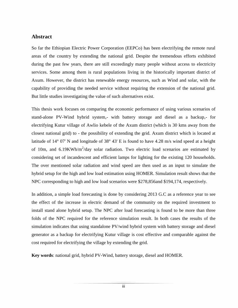
So far the Ethiopian Electric Power Corporation (EEPCo) has been electrifying the remote rural
areas of the country by extending the national grid. Despite the tremendous efforts exhibited
during the past few years, there are still exceedingly many people without access to electricity
services. Some among them is rural populations living in the historically important district of
Axum. However, the district has renewable energy resources, such as Wind and solar, with the
capability of providing the needed service without requiring the extension of the national grid.
But little studies investigating the value of such alternatives exist.
This thesis work focuses on comparing the economic performance of using various scenarios of
stand-alone PV-Wind hybrid system,- with battery storage and diesel as a backup,- for
electrifying Kutur village of Awlio kebele of the Axum district (which is 30 kms away from the
closest national grid) to - the possibility of extending the grid. Axum district which is located at
latitude of 14° 07' N and longitude of 38° 43' E is found to have 4.28 m/s wind speed at a height
of 10m, and 6.19KWh/m2/day solar radiation. Two electric load scenarios are estimated by
considering set of incandescent and efficient lamps for lighting for the existing 120 households.
The over mentioned solar radiation and wind speed are then used as an input to simulate the
hybrid setup for the high and low load estimation using HOMER. Simulation result shows that the
NPC corresponding to high and low load scenarios were $278,856and $194,174, respectively.
In addition, a simple load forecasting is done by considering 2013 G.C as a reference year to see
the effect of the increase in electric demand of the community on the required investment to
install stand alone hybrid setup. The NPC after load forecasting is found to be more than three
folds of the NPC required for the reference simulation result. In both cases the results of the
simulation indicates that using standalone PV/wind hybrid system with battery storage and diesel
generator as a backup for electrifying Kutur village is cost effective and comparable against the
cost required for electrifying the village by extending the grid.
Key words: national grid, hybrid PV-Wind, battery storage, diesel and HOMER.
iv
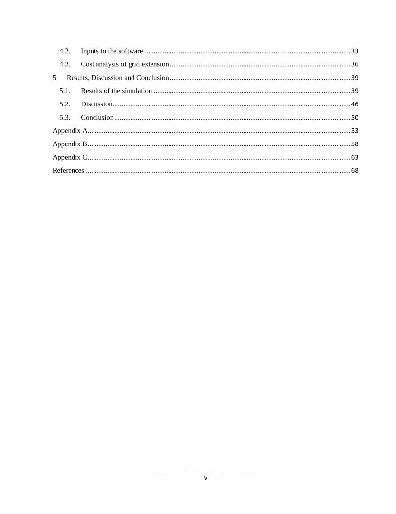
Table of Contents
DECLARATION .................................................................................................................................................. i
Acknowledgment ............................................................................................................................................ ii
Abstract .......................................................................................................................................................... iii
List of Tables ................................................................................................................................................. vi
List of Figures ............................................................................................................................................... vii
Acronyms ..................................................................................................................................................... viii
1. Introduction............................................................................................................................................. 1
1.1. Back ground of the study ................................................................................................................ 1
1.2. Statement of the problem ................................................................................................................ 3
1.3. Objectives of the study ................................................................................................................... 4
1.4. Methodology ................................................................................................................................... 4
2. Literature review and basic theory of system components ..................................................................... 6
2.1. Renewable energy technologies...................................................................................................... 6
2.2. Wind energy.................................................................................................................................... 6
2.2.1. Basic theory of wind ............................................................................................................... 6
2.2.2. Wind Data Analysis and Resource Estimation ....................................................................... 7
2.2.3. Analytical method for predicting long-term wind energy availability ................................... 8
2.2.4. Assessment of Wind potential .............................................................................................. 11
2.3. Solar energy .................................................................................................................................. 11
2.3.1. Basic theory of solar energy ................................................................................................. 11
2.3.2. Solar data analysis and resource estimation.......................................................................... 12
2.3.3. Measurement of sunshine duration and estimation of solar radiation .................................. 13
2.4. Hybrid system for rural electrification .......................................................................................... 14
3. Resource assessment and Load estimation ........................................................................................... 19
3.1. Assessment of solar radiation ....................................................................................................... 19
3.2. Load estimation ............................................................................................................................ 23
3.3. Population growth and load forecasting ....................................................................................... 27
4. Modeling of the hybrid system and cost analysis of grid extension ..................................................... 32
4.1. Modeling the hybrid system ......................................................................................................... 32
v
4.2. Inputs to the software .................................................................................................................... 33
4.3. Cost analysis of grid extension ..................................................................................................... 36
5. Results, Discussion and Conclusion ..................................................................................................... 39
5.1. Results of the simulation .............................................................................................................. 39
5.2. Discussion ..................................................................................................................................... 46
5.3. Conclusion .................................................................................................................................... 50
Appendix A ................................................................................................................................................... 53
Appendix B ................................................................................................................................................... 58
Appendix C ................................................................................................................................................... 63
References .................................................................................................................................................... 68
vi
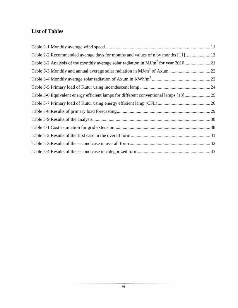
List of Tables
Table 2-1 Monthly average wind speed .......................................................................................... 11
Table 2-2 Recommended average days for months and values of n by months [11] ..................... 13
Table 3-2 Analysis of the monthly average solar radiation in MJ/m2 for year 2010 ...................... 21
Table 3-3 Monthly and annual average solar radiation in MJ/m2 of Axum ................................... 22
Table 3-4 Monthly average solar radiation of Axum in KWh/m2 .................................................. 22
Table 3-5 Primary load of Kutur using incandescent lamp ............................................................ 24
Table 3-6 Equivalent energy efficient lamps for different conventional lamps [18] ...................... 25
Table 3-7 Primary load of Kutur using energy efficient lamp (CFL) ............................................. 26
Table 3-8 Results of primary load forecasting ................................................................................ 29
Table 3-9 Results of the analysis .................................................................................................... 30
Table 4-1 Cost estimation for grid extension .................................................................................. 38
Table 5-2 Results of the first case in the overall form .................................................................... 41
Table 5-3 Results of the second case in overall form ..................................................................... 42
Table 5-4 Results of the second case in categorized form .............................................................. 43
vii
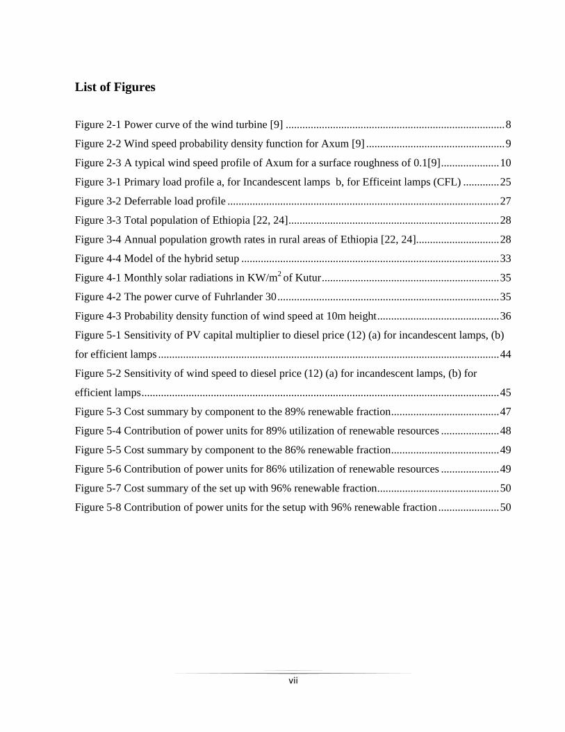
List of Figures
Figure 2-1 Power curve of the wind turbine [9] ............................................................................... 8
Figure 2-2 Wind speed probability density function for Axum [9] .................................................. 9
Figure 2-3 A typical wind speed profile of Axum for a surface roughness of 0.1[9] ..................... 10
Figure 3-1 Primary load profile a, for Incandescent lamps b, for Efficeint lamps (CFL) ............. 25
Figure 3-2 Deferrable load profile .................................................................................................. 27
Figure 3-3 Total population of Ethiopia [22, 24] ............................................................................ 28
Figure 3-4 Annual population growth rates in rural areas of Ethiopia [22, 24].............................. 28
Figure 4-4 Model of the hybrid setup ............................................................................................. 33
Figure 4-1 Monthly solar radiations in KW/m2 of Kutur ................................................................ 35
Figure 4-2 The power curve of Fuhrlander 30 ................................................................................ 35
Figure 4-3 Probability density function of wind speed at 10m height ............................................ 36
Figure 5-1 Sensitivity of PV capital multiplier to diesel price (12) (a) for incandescent lamps, (b)
for efficient lamps ........................................................................................................................... 44
Figure 5-2 Sensitivity of wind speed to diesel price (12) (a) for incandescent lamps, (b) for
efficient lamps ................................................................................................................................. 45
Figure 5-3 Cost summary by component to the 89% renewable fraction ....................................... 47
Figure 5-4 Contribution of power units for 89% utilization of renewable resources ..................... 48
Figure 5-5 Cost summary by component to the 86% renewable fraction ....................................... 49
Figure 5-6 Contribution of power units for 86% utilization of renewable resources ..................... 49
Figure 5-7 Cost summary of the set up with 96% renewable fraction............................................ 50
Figure 5-8 Contribution of power units for the setup with 96% renewable fraction ...................... 50
viii
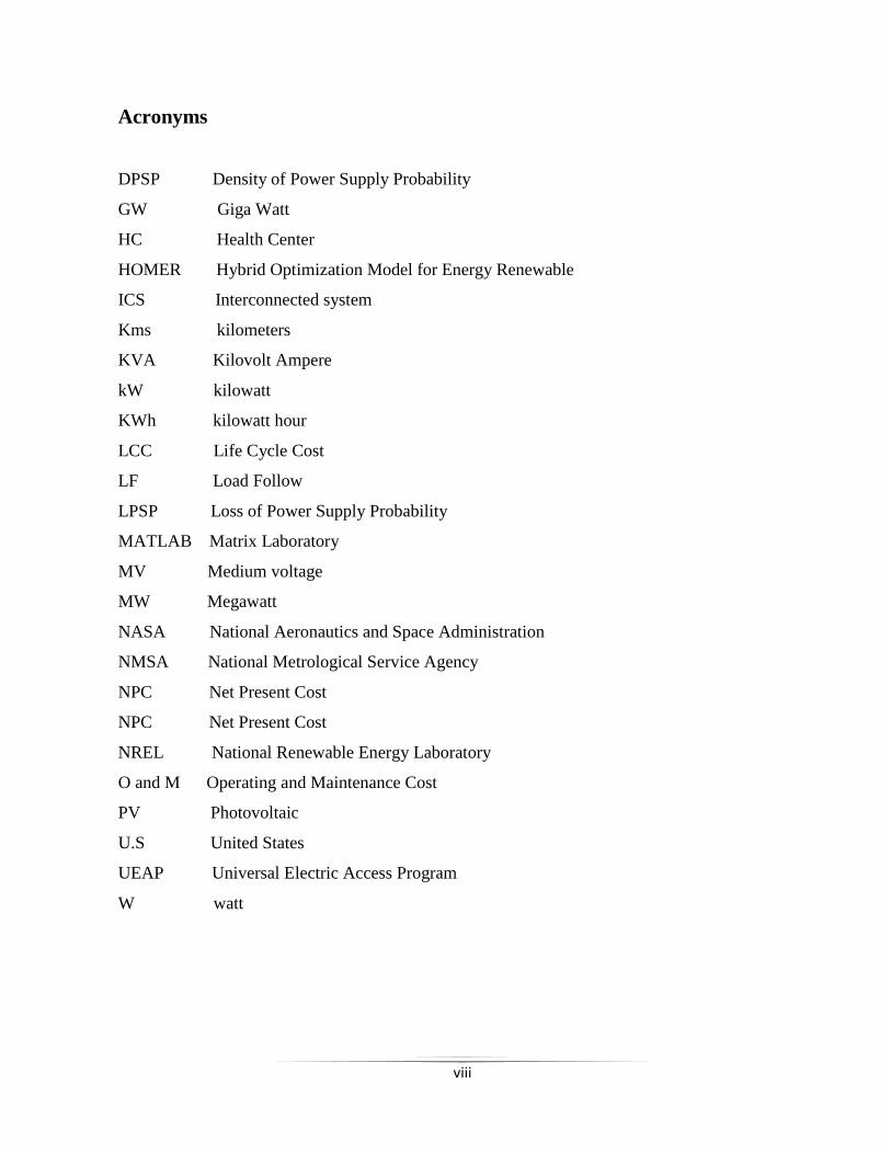
Acronyms
DPSP Density of Power Supply Probability
GW Giga Watt
HC Health Center
HOMER Hybrid Optimization Model for Energy Renewable
ICS Interconnected system
Kms kilometers
KVA Kilovolt Ampere
kW kilowatt
KWh kilowatt hour
LCC Life Cycle Cost
LF Load Follow
LPSP Loss of Power Supply Probability
MATLAB Matrix Laboratory
MV Medium voltage
MW Megawatt
NASA National Aeronautics and Space Administration
NMSA National Metrological Service Agency
NPC Net Present Cost
NPC Net Present Cost
NREL National Renewable Energy Laboratory
O and M Operating and Maintenance Cost
PV Photovoltaic
U.S United States
UEAP Universal Electric Access Program
W watt
1
1. Introduction
1.1. Back ground of the study
At the current rates of consumption, the reserves of oil and gas would be adequate to meet
demand for only another 41 and 67 years, respectively [1]. In addition to this, environmental
problems are growing dramatically due to a combination of several factors. These factors include
an increase in world population, energy consumption, and industrial activity. Solutions to such
environmental challenges require a policy aimed at long-term sustainable and clean development.
In this respect, renewable energy resources appear to be one of the most efficient and effective
solutions.
Despite over a century of investment in electric power systems, there are roughly 1.6 billion
people who lack access to electricity service, mainly in rural areas. While there are some open
questions regarding the precise cause and effect relationships between rural electrification and
human welfare, it is generally considered an important social, economic, and political priority to
provide electricity to all. Unfortunately, the very complicated links between electricity and
development are often obscured behind two idealized visions of rural electrification. Electricity is
often limited to meeting the basic needs of households, and those basic needs tend to be in
lighting, and entertainment. Electricity for productive activities or for welfare enhancing
community structures (e.g. schools or clinics) tends to lag behind basic household electrification
or sometimes is completely neglected in rural electrification objectives, making integration of
electrification into larger development goals difficult [3].
An estimate of Ethiopia‟s future electricity generation capacity includes more than 45000MW,
10000MW and 5000MW from hydropower, wind and geothermal resources, respectively [2].
Moreover, the country is a conducive geographic condition for solar power generation. Despite
the abundance of potential resources suitable for the energy sector development, the level of
electricity production has been poor. Currently, the national generation capacity stands at about
2000MW after the completion of Tekeze, Gilgel Gibe II and Tana-Beles with a capacity of
300MW, 420MW and 460MW, respectively. As a result, the overall access to electricity is
increased to 35% [2].

2
The government has also a plan to exploit energy from wind and geothermal to improve the
access to electricity to 50% in the coming five years [2]. The Ethiopian Electric Power
Corporation (EEPCo), a sole electric power producer and supplier in the country is therefore
endowed to fulfill the plan by increasing the production to 10,000MW in the near future including
the other renewable energy resources especially wind [2]. Moreover, there is also a program to
give electric access from solar to more than 150,000 households of remote rural areas of the
country with sufficient solar radiation resource in the coming five years [2].
The electric supply system throughout the country is interconnected system (ICS). Hence, most of
the remote rural areas which are located far off the grid do not have access to electricity. This
could be attributed to a set of problems, such as, insufficient generation capacity, high cost of
extending MV distribution line, lack of good planning and etcetra. Consequently, the rural areas
have been dependent on local solutions for electricity supply. These areas have been using
traditional biomass as source of energy for baking as well as cooking, and oil for lighting purpose.
The limited availability of biomass resource is forcing them to relay on an efficient energy
sources. These problems of the community and the current price increase in imported oil as well
as the negative effects of fossil fuels on the local and global environment motivates the search for
other alternatives.
The rural areas of Axum are among the villages of Ethiopia which are facing similar problems
due to the difficulty of giving electric access by extending the grid. But this can be minimized by
looking for alternative resources which can be used as a standalone to give electric access to the
community. Solar and wind can be the first option.
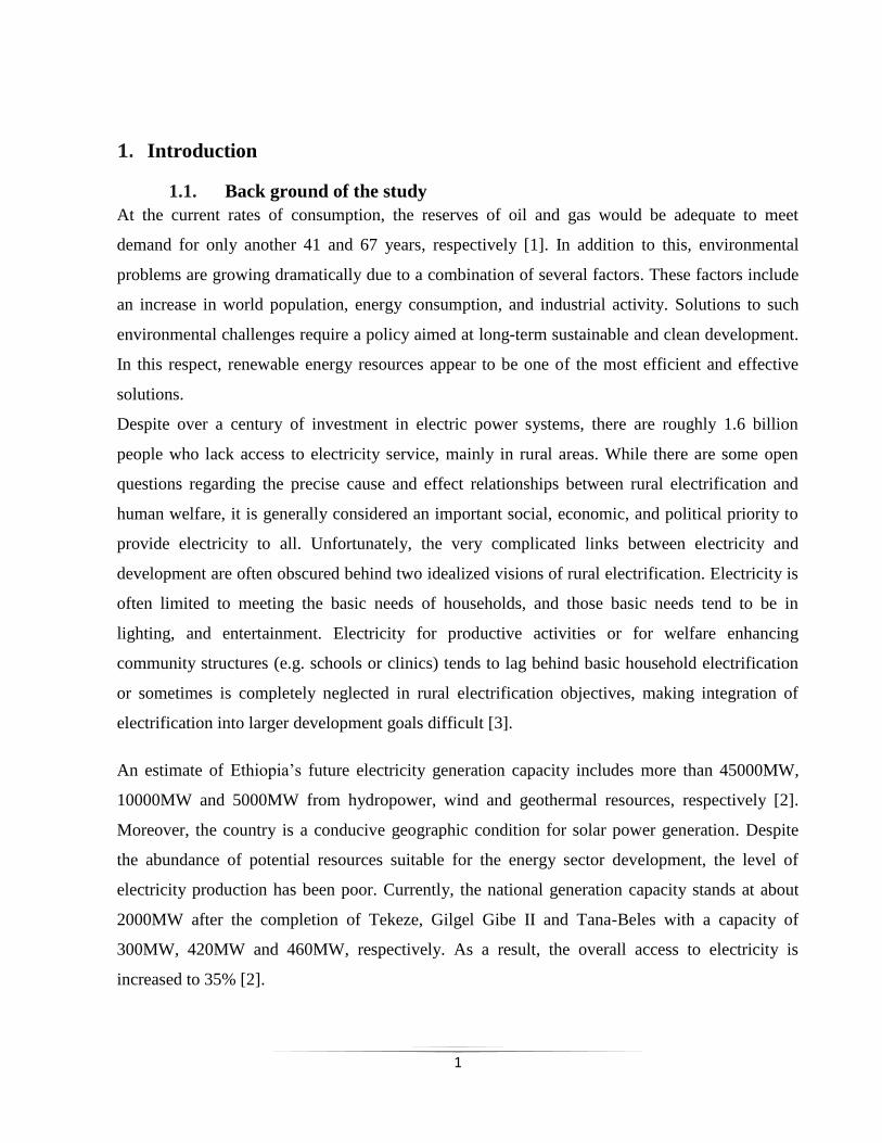
Figure 1-1 shows the settlement of the people of Kutur village found in Axum district which is
30kms away from the closest national grid. It also shows their traditional use of firewood for
baking. As it is shown on the figure, the area has a Tailor house. In addition to this, it has small
shops which supply the daily goods needed by the community. It also shows the traditional
“mitad” or stove used for baking bread and “Injera” (a flat pancake type bread). So far, the people
of this area have been using firewood as a main source of energy as shown in the figure below.
Hence, the greenery in the vicinity is highly exposed to deforestation. Therefore, this work is
conducted to show the possibility of using PV-wind hybrid system for electrifying the village. It
3
also shows its significance in improving the life of inhabitants and fertility of the land by reducing
deforestation caused by the people of the area.
Figure 1-1 picture taken from Kutur village
1.2. Statement of the problem
Rural electrification is the basic issue of the government of Ethiopia for assuring the agricultural
lead industrialization. As a result, the Ethiopian Electric Power Corporation is trying to electrify
some rural areas which are even more than 120 kms away from a nearby substation or from
existing MV distribution line by expending much money to extend the existing national grid even
though most of the rural areas are potentially rich in renewable energy resources. These resources
can be used as a stand-alone with minimum cost as compared against the cost required for
extending the grid.
Most of the remote rural areas of the country are still without electricity access. Likewise the rural
people of Axum district which are far away from the national grid are also facing the same
problem; and they did not get electric access from the grid so far. As the consequence; the people
of these areas are still confined to using traditional biomass as a source of energy for cooking
their food, and imported oil for lighting. As a result, they are exposed to health problems caused
by smokes while also contributing to deforestation. Therefore, it is important to investigate the
potential role of various electrification options.
4
Moreover, supplying energy from hybrid system will help them improve their life style as well as
reduce deforestation. In addition, it will contribute a lot to the achievement of agricultural lead
industrialization by minimizing the expense of Universal Electric Access Program.
1.3. Objectives of the study
General objective
In this thesis, assessment of resource potential and modeling of the Stand- alone PV/Wind Hybrid
System for electrifying rural areas in the Axum region will be done.
Specific objectives
The specific objectives of this thesis work are
To select the best optimized hybrid model for providing electricity to the community by
considering its overall installation cost, contribution of renewable energy sources and
energy cost per kWh.
To analyze the power and energy demand of the society of the selected areas by
considering the basic needs of the people.
To select appropriate solar modules, wind turbines and batteries depending on the energy
demand for the individual sites.
To compare the investment cost of the hybrid system against the cost required to electrify
the areas by extending the national grid.
To determine the demand of the community at the life span of the project through load
forecasting.
1.4. Methodology
As mentioned above, this research is mainly concerned to looking in to better option of energy
sources to electrify villages in remote areas of Ethiopia which are far-off from the existing
national grid by comparing against the cost needed to extend the national grid. The main concern
is the assessment of resource potential and modeling of the stand-alone hybrid system by

5
analyzing the data taken from different data sources. These are done through reviewing literatures
related to hybrid systems, and adopting different concepts and methodologies as required.
Primary data:
The primary work is field data collection, which includes data of the number of households and
site observation to evaluate their living style. The field data supported by photographs to show
equipments used by the community, as well as their daily life style and activity related to energy
consumption. The power demand of each house hold has been estimated based on the need of the
community and application of numerical data using Microsoft excel spread sheet. In addition, a
simple exponential load forecasting method is used to consider the effect of change of electric
load of the community with in the life span of the project which is 25 years.
Secondary Data:
The wind speed and solar radiation of the selected sites are collated from different sources such
as: the national metrological service agency of Ethiopia (NMSA), National Aeronautics and
Space Administration (NASA), previous works by other scholars and others. Then the data
collected from NMSA are analyzed using theoretically proved formulas. Moreover, the data
needed for calculating the cost of extending the grid is taken from EEPCO, and it is analyzed
using Microsoft excel spread sheet.
Finally the hybrid system is modeled and simulated using HOMER software based on the primary
and secondary analyzed data to get the best optimized solution for both load estimations which
are estimated by considering incandescent and CFL for lighting.
6
2. Literature review and basic theory of system components
2.1. Renewable energy technologies
The sun generates its energy by nuclear fusion of hydrogen nuclei to helium. Sunlight is the main
source of energy to the surface of the earth that can be harnessed via a variety of natural and
synthetic processes. Basically all the forms of energy in the world as we know it are solar in
origin. Oil, coal, natural gas, and wood were originally produced by photosynthetic processes,
followed by complex chemical reactions in which decaying vegetation was subjected to very high
temperatures and pressures over a long period of time. Even the energy of the wind has a solar
origin, since it is caused by differences in temperature in various regions of the earth [5].
Renewable energy systems are important to decrease environmental pollution, and this can be
achieved by the reduction of air emissions due to the substitution of conventional energy
resources. The most important effects of air pollutants on the human and natural environment are
their impact on the public health, agriculture, and ecosystems. The financial impact of these
effects can be measured easily by relating to tradable goods. In addition to these factors, the
consumption of renewable energy resources does not result in the depletion of resources [6]. And
the instable energy provision which is the major problem of these energy resources can then be
solved by using hybrid energy supply systems.
2.2. Wind energy
2.2.1. Basic theory of wind
Global wind is caused by pressure differences across the earth‟s surface due to the uneven heating
of the earth by solar radiation. The uneven heating of the earth resulted in circulation of the
atmosphere which is greatly influenced by the effects of the rotation of the earth. In addition,
variations in the circulation can be caused due to seasonal variations in the distribution of solar
energy.
This wind blows predominately in the horizontal plane, responding to horizontal pressure
gradients since the pressure gradient force in the vertical direction is usually cancelled by the
downward gravitational force. At the same time, there are forces that struggle to mix the different
temperature and pressure air masses distributed across the earth„s surface. Similarly, inertia of the
7
air, the earth„s rotation, and friction with the earth‟s surface (resulting in turbulence), affect the
atmospheric winds. Wind speed can also vary with height above the ground, geographical
location and time.
These variations of wind speed with time can be categorized as inter-annual, annual, diurnal and
short-term. The Inter-annual wind speed variation can have a large effect on long-term wind
turbine production since it occurs over time scales greater than one year. Diurnal variation can be
defined as an increase in wind speed during the day with the wind speeds lowest during the hours
from midnight to sunrise. This is caused due to differential heating of the earth‟s surface during
the daily radiation cycle. Even though daily variations in solar radiation are responsible for
diurnal wind variations in temperate latitudes over relatively flat land areas, it can also vary with
location and altitude above sea level. The largest diurnal changes generally occur in spring and
summer, and the smallest in winter. Similarly, the short term wind speed variation can be defined
as the mean variations over time intervals of 10 minutes or less, and it includes turbulence and
gusts [7].
2.2.2. Wind Data Analysis and Resource Estimation
Wind resource or power production potential of a particular site can be evaluated by direct and
statistical techniques. Wind is produced due to temperature variation which results in pressure
variation, and it blows from high pressure to low pressure area. The power from wind can be
calculated using the formula
3
21 AUP Eqn. 2-1
Where: P is wind power
A is Rotor area
U is wind speed
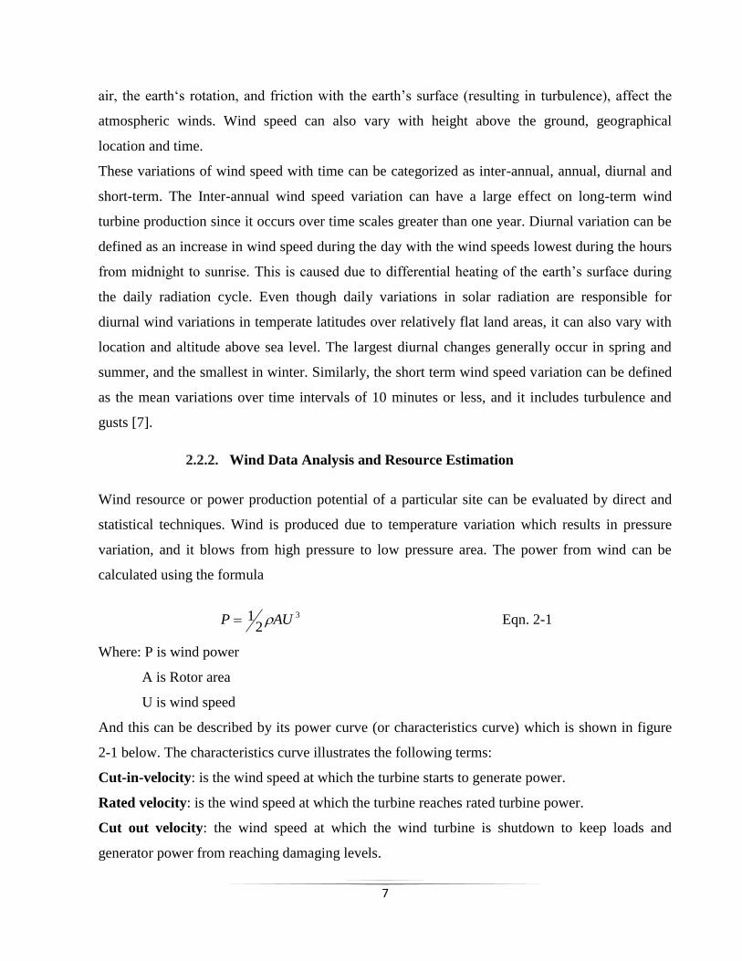
And this can be described by its power curve (or characteristics curve) which is shown in figure
2-1 below. The characteristics curve illustrates the following terms:
Cut-in-velocity: is the wind speed at which the turbine starts to generate power.
Rated velocity: is the wind speed at which the turbine reaches rated turbine power.
Cut out velocity: the wind speed at which the wind turbine is shutdown to keep loads and
generator power from reaching damaging levels.
8
Figure 2-1 Power curve of the wind turbine [9]
The power density can be calculated as
N
i
iUNA
P
1
312
1 Eqn. 2-2
This is the formula used to calculate the most approximate value for power density since the cubic
of average speed is different from the sum of the cubic of individual speeds [8].
2.2.3. Analytical method for predicting long-term wind energy availability
After the wind speed data has been recorded for more than five years, the distribution probability
can be used to predict a future wind speed availability and elucidate: (1) the period without wind,
or when the wind is too weak to start up the wind turbines; (2) the range of most likely wind
speeds; and (3) the nominal power output and the probabilities associated with various outputs
[3]. The wind data can then be analyzed using two different analysis methods. These are the
Rayleigh which uses the mean wind speed as a parameter, and Weibull which uses two
parameters for statistical analysis.
The Weibull probability distribution (h (v)) is a mathematical expression which has been found to
provide a good approximation to the measured wind speed distribution.
9
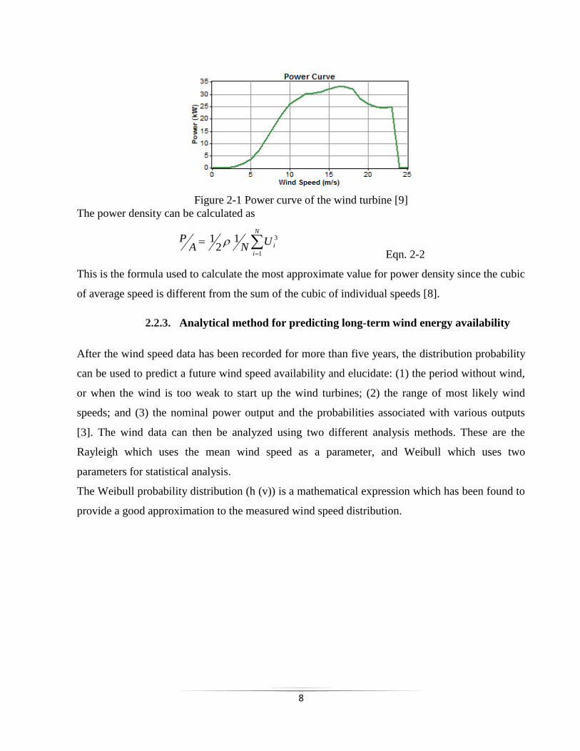
Figure 2-2 Wind speed probability density function for Axum [9]
A Weibull distribution graph is usually used to describe wind variation over a certain period of
time at a particular site. Figure 2-2 shows a typical distribution plot for wind speed data based on
wind speed measured five times every day for three years, 2007–2011, in Axum. As can be seen
in the graph, the mean wind speed is about 4.83 m/s. The mean wind speed can be obtained by
summing up the products of each wind speed interval and the probability of getting that wind
speed.
The distribution of wind is expressed by Weibull distribution which is called a Raleigh
distribution for K=2 [3, 10]. It is given by equations (2-3 to 2-5).
2
2 4exp
2)(
v
v
v
vvf
Eqn. 2-3
2
4exp1)(
v
vVvprob
Eqn. 2-4
2
4exp)(
v
vVvprob
Eqn. 2-5
Where, f (v)= Weibull probability density function of wind distribution
v = mean wind speed (m/s)
v=instantaneous wind speed (m/s)
prob(v<=V)=probability of instantaneous wind speed is less than V
prob(v<=V)=probability of instantaneous wind speed is greater than V
10
Wind speeds are always measured at 10 m height anemometer. But, wind turbines are installed at
higher elevations at which the wind speed is completely different from the 10 m measurement.
This variation of wind speed with height can be expressed with equation 2-6 [3, 10].
00
lnlnz
zzv
z
zzv r
r Eqn.2-6
Where: Zr Reference height (m)
Z Height where wind speed is to be determined (m)
Z0 Measure of surface roughness (0.1 to 0.25 for crop land)
zv Wind speed at height of Z m (m/s)
rzv Wind speed at the reference height (m/s)
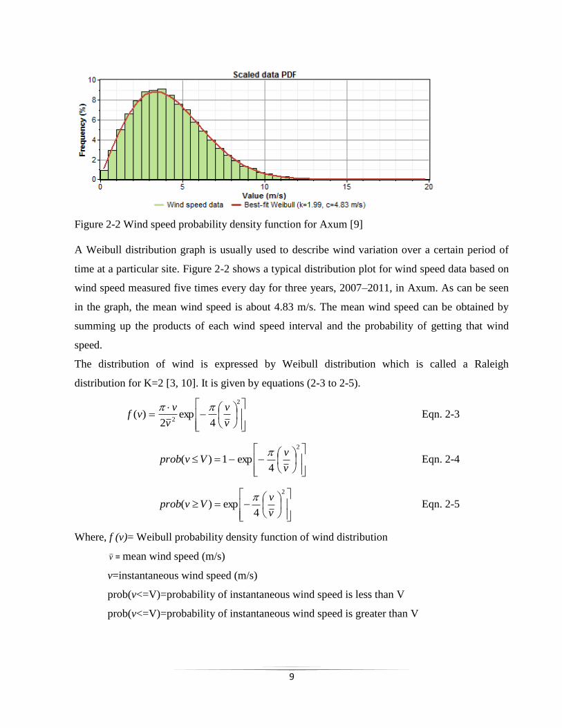
Figure 2-3 A typical wind speed profile of Axum for a surface roughness of 0.1[9]
From the relationship given in equation 2-6 it can be observed that the wind speed increases with
height and therefore a higher tower captures more wind energy. If the wind speed 𝑣(𝑧𝑟) at a
certain reference height 𝑧𝑟 above a surface with a known roughness length (zo); then, the wind
speed 𝑣(𝑧) at a height of z can be determined using equation 2-6 above [6]. The figure shown
above illustrates a typical wind speed profile for a surface roughness length of 0.1 of the selected
site.
11
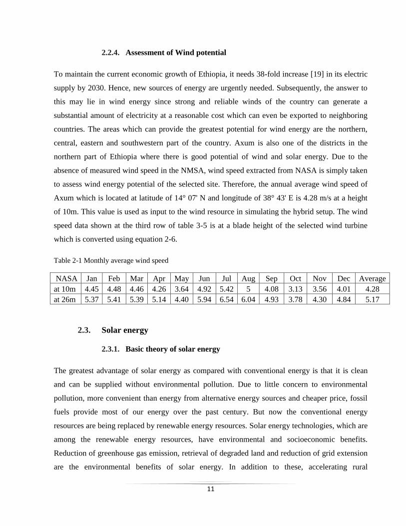
2.2.4. Assessment of Wind potential
To maintain the current economic growth of Ethiopia, it needs 38-fold increase [19] in its electric
supply by 2030. Hence, new sources of energy are urgently needed. Subsequently, the answer to
this may lie in wind energy since strong and reliable winds of the country can generate a
substantial amount of electricity at a reasonable cost which can even be exported to neighboring
countries. The areas which can provide the greatest potential for wind energy are the northern,
central, eastern and southwestern part of the country. Axum is also one of the districts in the
northern part of Ethiopia where there is good potential of wind and solar energy. Due to the
absence of measured wind speed in the NMSA, wind speed extracted from NASA is simply taken
to assess wind energy potential of the selected site. Therefore, the annual average wind speed of
Axum which is located at latitude of 14° 07' N and longitude of 38° 43' E is 4.28 m/s at a height
of 10m. This value is used as input to the wind resource in simulating the hybrid setup. The wind
speed data shown at the third row of table 3-5 is at a blade height of the selected wind turbine
which is converted using equation 2-6.
Table 2-1 Monthly average wind speed
NASA Jan Feb Mar Apr May Jun Jul Aug Sep Oct Nov Dec Average
at 10m 4.45 4.48 4.46 4.26 3.64 4.92 5.42 5 4.08 3.13 3.56 4.01 4.28
at 26m 5.37 5.41 5.39 5.14 4.40 5.94 6.54 6.04 4.93 3.78 4.30 4.84 5.17
2.3. Solar energy
2.3.1. Basic theory of solar energy
The greatest advantage of solar energy as compared with conventional energy is that it is clean
and can be supplied without environmental pollution. Due to little concern to environmental
pollution, more convenient than energy from alternative energy sources and cheaper price, fossil
fuels provide most of our energy over the past century. But now the conventional energy
resources are being replaced by renewable energy resources. Solar energy technologies, which are
among the renewable energy resources, have environmental and socioeconomic benefits.
Reduction of greenhouse gas emission, retrieval of degraded land and reduction of grid extension
are the environmental benefits of solar energy. In addition to these, accelerating rural
12
electrification, creation of employment opportunities and improving diversification and stability
of energy supply are its socioeconomic benefits [5].
2.3.2. Solar data analysis and resource estimation
Solar radiation data are available in several forms. There are two popularly used measuring
instruments to know the amount of radiation incident on a horizontal surface of a specific
(selected) area. Among these the one which measures the sun shine duration is used by the
national metrological service agency of Ethiopia. Therefore, some mechanism has to be used to
convert the values of the measured data to the required solar radiation if someone wants to know
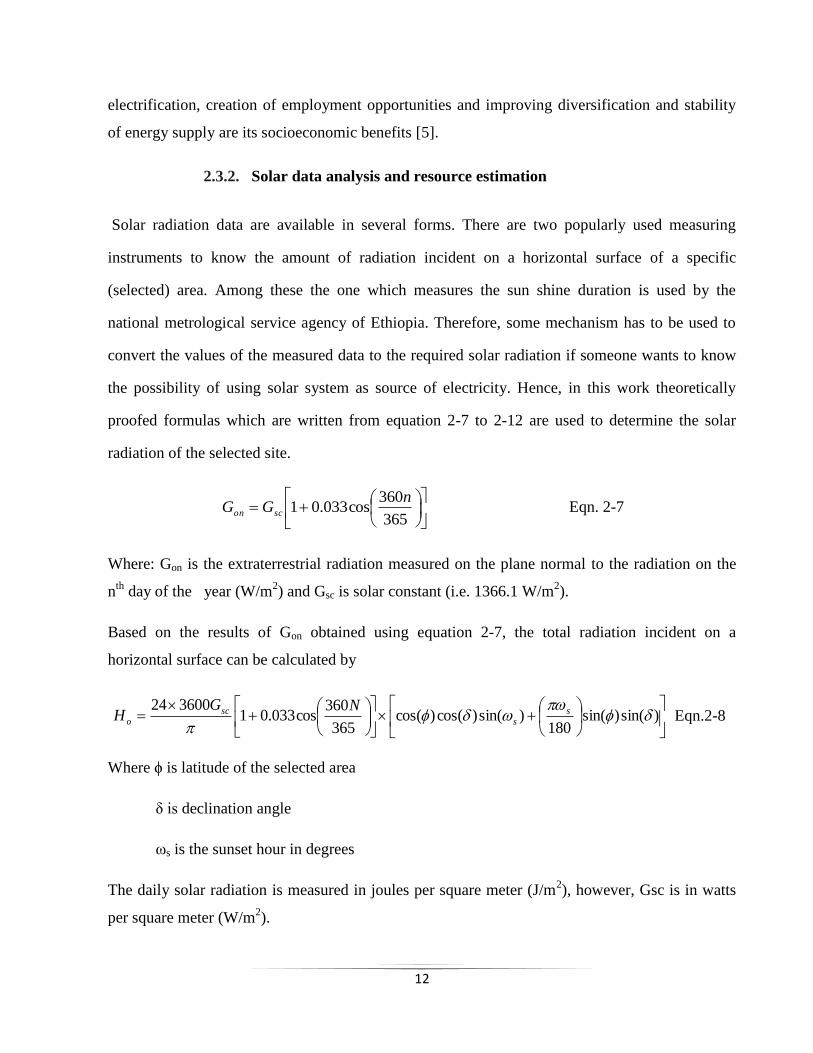
the possibility of using solar system as source of electricity. Hence, in this work theoretically
proofed formulas which are written from equation 2-7 to 2-12 are used to determine the solar
radiation of the selected site.
365
360cos033.01
nGG scon Eqn. 2-7
Where: Gon is the extraterrestrial radiation measured on the plane normal to the radiation on the
nth
day of the year (W/m2) and Gsc is solar constant (i.e. 1366.1 W/m
2).
Based on the results of Gon obtained using equation 2-7, the total radiation incident on a
horizontal surface can be calculated by
)sin()sin(
180)sin()cos()cos(
365
360cos033.01
360024
s
s
sc
o
NGH Eqn.2-8
Where ϕ is latitude of the selected area
δ is declination angle
ωs is the sunset hour in degrees
The daily solar radiation is measured in joules per square meter (J/m2), however, Gsc is in watts
per square meter (W/m2).
13
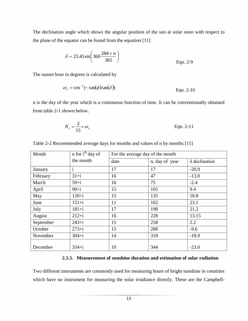
The declination angle which shows the angular position of the sun at solar noon with respect to
the plane of the equator can be found from the equation [11]
365
284360sin45.23
n
Eqn. 2-9
The sunset hour in degrees is calculated by
)tantan(cos 1
s Eqn. 2-10
n is the day of the year which is a continuous function of time. It can be conventionally obtained
from table 2-1 shown below.
ssN 15
2 Eqn. 2-11
Table 2-2 Recommended average days for months and values of n by months [11]
Month n for ith
day of
the month
For the average day of the month
date n, day of year δ declination
January i 17 17 -20.9
February 31+i 16 47 -13.0
March 59+i 16 75 -2.4
April 90+i 15 105 9.4
May 120+i 15 135 18.8
June 151+i 11 162 23.1
July 181+i 17 198 21.2
August 212+i 16 228 13.15
September 243+i 15 258 2.2
October 273+i 15 288 -9.6
November 304+i 14 318 -18.9
December 334+i 10 344 -23.0
2.3.3. Measurement of sunshine duration and estimation of solar radiation
Two different instruments are commonly used for measuring hours of bright sunshine in countries
which have no instrument for measuring the solar irradiance directly. These are the Campbell-
14
Stokes sunshine recorder which uses a solid glass sphere of approximately 10 cm as a lens that
produces an image of the sun on the opposite surface of the sphere, and a photoelectric sunshine
recorder.
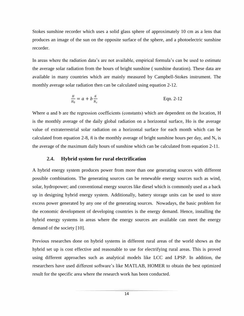
In areas where the radiation data‟s are not available, empirical formula‟s can be used to estimate
the average solar radiation from the hours of bright sunshine ( sunshine duration). These data are
available in many countries which are mainly measured by Campbell-Stokes instrument. The
monthly average solar radiation then can be calculated using equation 2-12.
𝐻
𝐻0= 𝑎 + 𝑏
𝑛
𝑁𝑠 Eqn. 2-12
Where ɑ and b are the regression coefficients (constants) which are dependent on the location, H
is the monthly average of the daily global radiation on a horizontal surface, Ho is the average
value of extraterrestrial solar radiation on a horizontal surface for each month which can be
calculated from equation 2-8, 𝑛 is the monthly average of bright sunshine hours per day, and Ns is
the average of the maximum daily hours of sunshine which can be calculated from equation 2-11.
2.4. Hybrid system for rural electrification
A hybrid energy system produces power from more than one generating sources with different
possible combinations. The generating sources can be renewable energy sources such as wind,
solar, hydropower; and conventional energy sources like diesel which is commonly used as a back
up in designing hybrid energy system. Additionally, battery storage units can be used to store
excess power generated by any one of the generating sources. Nowadays, the basic problem for
the economic development of developing countries is the energy demand. Hence, installing the
hybrid energy systems in areas where the energy sources are available can meet the energy
demand of the society [10].
Previous researches done on hybrid systems in different rural areas of the world shows as the
hybrid set up is cost effective and reasonable to use for electrifying rural areas. This is proved
using different approaches such as analytical models like LCC and LPSP. In addition, the
researchers have used different software‟s like MATLAB, HOMER to obtain the best optimized
result for the specific area where the research work has been conducted.
15
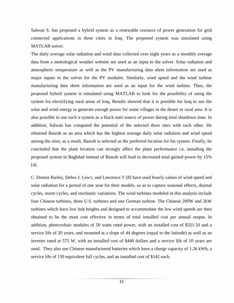
Salwan S. has proposed a hybrid system as a renewable resource of power generation for grid
connected applications in three cities in Iraq. The proposed system was simulated using
MATLAB solver.
The daily average solar radiation and wind data collected over eight years as a monthly average
data from a metrological weather website are used as an input to the solver. Solar radiation and
atmospheric temperature as well as the PV manufacturing data sheet information are used as
major inputs to the solver for the PV modules. Similarly, wind speed and the wind turbine
manufacturing data sheet information are used as an input for the wind turbine. Then, the
proposed hybrid system is simulated using MATLAB to look for the possibility of using the
system for electrifying rural areas of Iraq. Results showed that it is possible for Iraq to use the
solar and wind energy to generate enough power for some villages in the desert or rural area. It is
also possible to use such a system as a black start source of power during total shutdown time. In
addition, Salwan has compared the potential of the selected three sites with each other. He
obtained Basrah as an area which has the highest average daily solar radiation and wind speed
among the sites; as a result, Basrah is selected as the preferred location for his system. Finally, he
concluded that the plant location can strongly affect the plant performance i.e. installing the
proposed system in Baghdad instead of Basrah will lead to decreased total gained power by 15%
[4].
C. Dennis Barley, Debra J. Lew1, and Lawrence T [8] have used hourly values of wind speed and
solar radiation for a period of one year for their models, so as to capture seasonal effects, diurnal
cycles, storm cycles, and stochastic variations. The wind turbines modeled in this analysis include
four Chinese turbines, three U.S. turbines and one German turbine. The Chinese 200W and 2kW
turbines which have low hub heights and designed to accommodate the low wind speeds are then
obtained to be the most cost effective in terms of total installed cost per annual output. In
addition, photovoltaic modules of 50 watts rated power, with an installed cost of $321.50 and a
service life of 20 years, and mounted at a slope of 44 degrees (equal to the latitude) as well as an
inverter rated at 575 W, with an installed cost of $440 dollars and a service life of 10 years are
used. They also use Chinese manufactured batteries which have a charge capacity of 1.26 kWh, a
service life of 150 equivalent full cycles, and an installed cost of $142 each.
16
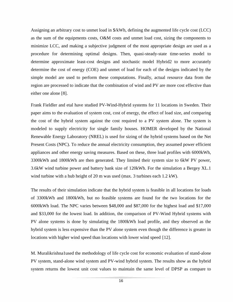
Assigning an arbitrary cost to unmet load in $/kWh, defining the augmented life cycle cost (LCC)
as the sum of the equipments costs, O&M costs and unmet load cost, sizing the components to
minimize LCC, and making a subjective judgment of the most appropriate design are used as a
procedure for determining optimal designs. Then, quasi-steady-state time-series model to
determine approximate least-cost designs and stochastic model Hybrid2 to more accurately
determine the cost of energy (COE) and unmet of load for each of the designs indicated by the
simple model are used to perform these computations. Finally, actual resource data from the
region are processed to indicate that the combination of wind and PV are more cost effective than
either one alone [8].
Frank Fieldler and etal have studied PV-Wind-Hybrid systems for 11 locations in Sweden. Their
paper aims to the evaluation of system cost, cost of energy, the effect of load size, and comparing
the cost of the hybrid system against the cost required to a PV system alone. The system is
modeled to supply electricity for single family houses. HOMER developed by the National
Renewable Energy Laboratory (NREL) is used for sizing of the hybrid systems based on the Net
Present Costs (NPC). To reduce the annual electricity consumption, they assumed power efficient
appliances and other energy saving measures. Based on these, three load profiles with 6000kWh,
3300kWh and 1800kWh are then generated. They limited their system size to 6kW PV power,
3.6kW wind turbine power and battery bank size of 120kWh. For the simulation a Bergey XL.1
wind turbine with a hub height of 20 m was used (max. 3 turbines each 1.2 kW).
The results of their simulation indicate that the hybrid system is feasible in all locations for loads
of 3300kWh and 1800kWh, but no feasible systems are found for the two locations for the
6000kWh load. The NPC varies between $48,000 and $87,000 for the highest load and $17,000
and $33,000 for the lowest load. In addition, the comparison of PV-Wind Hybrid systems with
PV alone systems is done by simulating the 1800kWh load profile, and they observed as the
hybrid system is less expensive than the PV alone system even though the difference is greater in
locations with higher wind speed than locations with lower wind speed [12].
M. Muralikrishna1used the methodology of life cycle cost for economic evaluation of stand-alone
PV system, stand-alone wind system and PV-wind hybrid system. The results show as the hybrid
system returns the lowest unit cost values to maintain the same level of DPSP as compare to
17
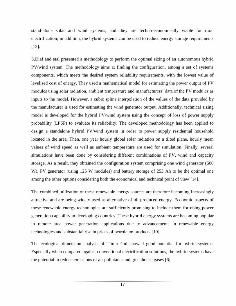
stand-alone solar and wind systems, and they are techno-economically viable for rural
electrification; in addition, the hybrid systems can be used to reduce energy storage requirements
[13].
S.Diaf and etal presented a methodology to perform the optimal sizing of an autonomous hybrid
PV/wind system. The methodology aims at finding the configuration, among a set of systems
components, which meets the desired system reliability requirements, with the lowest value of
levelised cost of energy. They used a mathematical model for estimating the power output of PV
modules using solar radiation, ambient temperature and manufacturers‟ data of the PV modules as
inputs to the model. However, a cubic spline interpolation of the values of the data provided by
the manufacturer is used for estimating the wind generator output. Additionally, technical sizing
model is developed for the hybrid PV/wind system using the concept of loss of power supply
probability (LPSP) to evaluate its reliability. The developed methodology has been applied to
design a standalone hybrid PV/wind system in order to power supply residential household
located in the area. Then, one year hourly global solar radiation on a tilted plane, hourly mean
values of wind speed as well as ambient temperature are used for simulation. Finally, several
simulations have been done by considering different combinations of PV, wind and capacity
storage. As a result, they obtained the configuration system comprising one wind generator (600
W), PV generator (using 125 W modules) and battery storage of 253 Ah to be the optimal one
among the other options considering both the economical and technical point of view [14].
The combined utilization of these renewable energy sources are therefore becoming increasingly
attractive and are being widely used as alternative of oil produced energy. Economic aspects of
these renewable energy technologies are sufficiently promising to include them for rising power
generation capability in developing countries. These hybrid energy systems are becoming popular
in remote area power generation applications due to advancements in renewable energy
technologies and substantial rise in prices of petroleum products [10].
The ecological dimension analysis of Timur Gul showed good potential for hybrid systems.
Especially when compared against conventional electrification solutions, the hybrid systems have
the potential to reduce emissions of air pollutants and greenhouse gases [6].

18
The main components of the hybrid system for this thesis work are: photovoltaic and wind. In
addition to these, storage battery and diesel are used as a backup system to fill the gap resulted
due to less production of energy from PV and wind.
19
3. Resource assessment and Load estimation
3.1. Assessment of solar radiation
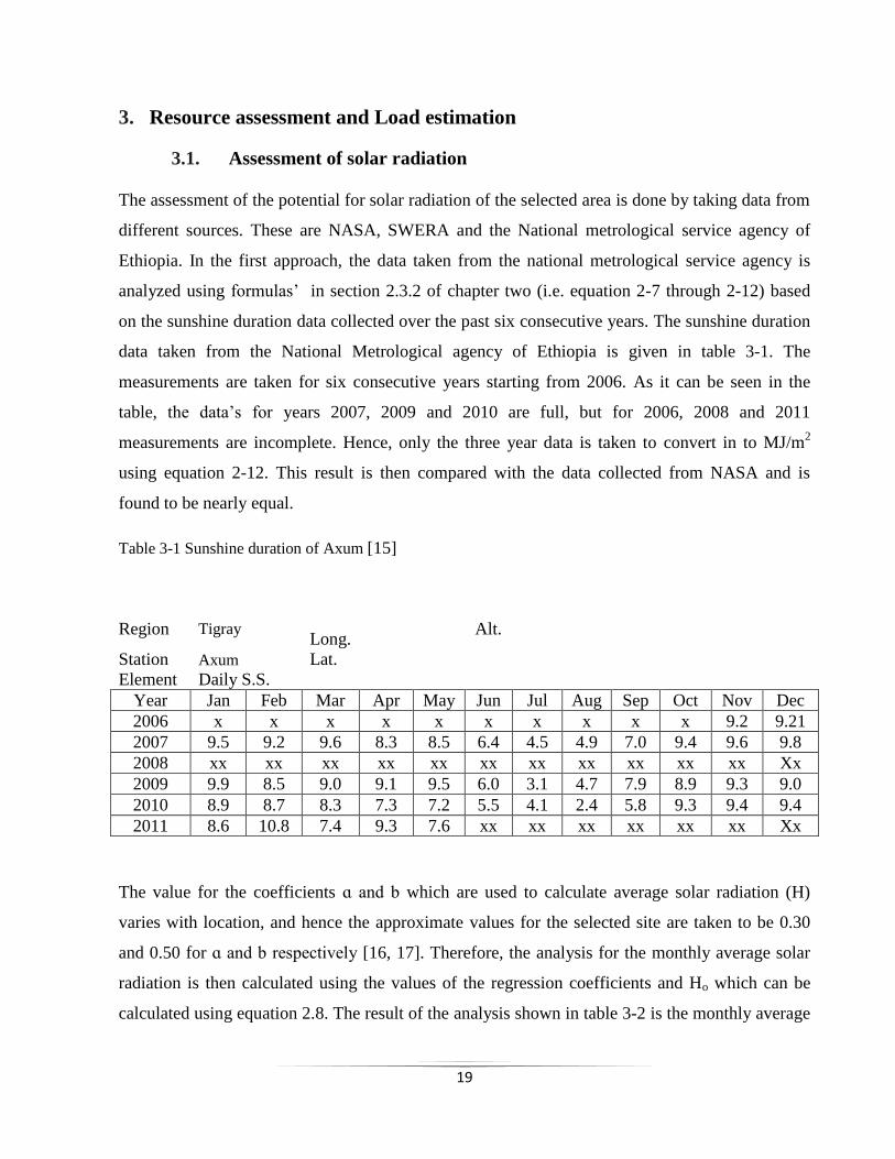
The assessment of the potential for solar radiation of the selected area is done by taking data from
different sources. These are NASA, SWERA and the National metrological service agency of
Ethiopia. In the first approach, the data taken from the national metrological service agency is
analyzed using formulas‟ in section 2.3.2 of chapter two (i.e. equation 2-7 through 2-12) based
on the sunshine duration data collected over the past six consecutive years. The sunshine duration
data taken from the National Metrological agency of Ethiopia is given in table 3-1. The
measurements are taken for six consecutive years starting from 2006. As it can be seen in the
table, the data‟s for years 2007, 2009 and 2010 are full, but for 2006, 2008 and 2011
measurements are incomplete. Hence, only the three year data is taken to convert in to MJ/m2
using equation 2-12. This result is then compared with the data collected from NASA and is
found to be nearly equal.
Table 3-1 Sunshine duration of Axum [15]
The value for the coefficients ɑ and b which are used to calculate average solar radiation (H)
varies with location, and hence the approximate values for the selected site are taken to be 0.30
and 0.50 for ɑ and b respectively [16, 17]. Therefore, the analysis for the monthly average solar
radiation is then calculated using the values of the regression coefficients and Ho which can be
calculated using equation 2.8. The result of the analysis shown in table 3-2 is the monthly average
Region Tigray
Long. Alt.
Station Axum
Lat.
Element Daily S.S.
Year Jan Feb Mar Apr May Jun Jul Aug Sep Oct Nov Dec
2006 x x x x x x x x x x 9.2 9.21
2007 9.5 9.2 9.6 8.3 8.5 6.4 4.5 4.9 7.0 9.4 9.6 9.8
2008 xx xx xx xx xx xx xx xx xx xx xx Xx
2009 9.9 8.5 9.0 9.1 9.5 6.0 3.1 4.7 7.9 8.9 9.3 9.0
2010 8.9 8.7 8.3 7.3 7.2 5.5 4.1 2.4 5.8 9.3 9.4 9.4
2011 8.6 10.8 7.4 9.3 7.6 xx xx xx xx xx xx Xx
20
solar radiation in MJ/m2
for the sunshine duration measured in 2010. In the same manner, the
monthly average solar radiation for the hours of bright sunshine measured in 2007 and 2009 is
converted in to MJ/m2. Finally the monthly average solar radiation of the selected site based on
the three year fully measured data is summarized and obtained to be as shown in table 3-3.
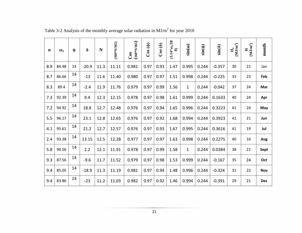
The symbols used in table 3-2 represent the measured and calculated values which are used to
analyze the extraterrestrial radiation (i.e. Ho) and the solar radiation for the location. n and ϕ
represents measured sunshine duration and the latitude angle of the area respectively. However,
the symbols δ, ωs and Ns indicates the calculated values for declination angle, sunset angle and
day length which are obtained using equations 2-9, 2-10 and 2-11 respectively.
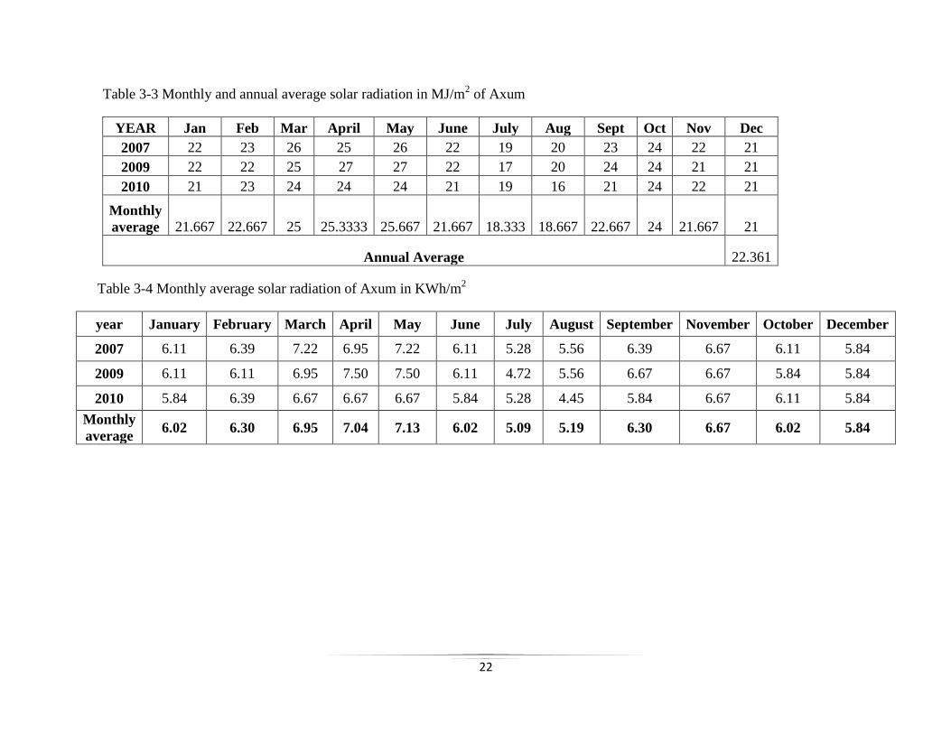
The monthly solar radiation data for each month of the years with full measured hours of bright
sunshine are shown in table 3-3. This table also shows monthly and annual average solar radiation
in MJ/m2 of Axum.
21
Table 3-2 Analysis of the monthly average solar radiation in MJ/m2 for year 2010
n ωs ϕ δ N
(360
*N
/36
5)
Cos
(36
0*
N/3
65)
Cos
(ϕ)
Cos
(δ)
(3.1
4*
ωs/
18
0)
sin
(ω)
sin
(ϕ)
sin
(δ)
Ho
(MJ
/m2)
H
(MJ
/m2)
mon
th
8.9 84.48 14 -20.9 11.3 11.11 0.981 0.97 0.93 1.47 0.995 0.244 -0.357 30 21 Jan
8.7 86.66 14
-13 11.6 11.40 0.980 0.97 0.97 1.51 0.998 0.244 -0.225 33 23 Feb
8.3 89.4 14
-2.4 11.9 11.76 0.979 0.97 0.99 1.56 1 0.244 -0.042 37 24 Mar
7.3 92.39 14
9.4 12.3 12.15 0.978 0.97 0.98 1.61 0.999 0.244 0.1633 40 24 Apr
7.2 94.92 14
18.8 12.7 12.48 0.976 0.97 0.94 1.65 0.996 0.244 0.3223 41 24 May
5.5 96.17 14
23.1 12.8 12.65 0.976 0.97 0.92 1.68 0.994 0.244 0.3923 41 21 Jun
4.1 95.61 14
21.2 12.7 12.57 0.976 0.97 0.93 1.67 0.995 0.244 0.3616 41 19 Jul
2.4 93.38 14
13.15 12.5 12.28 0.977 0.97 0.97 1.63 0.998 0.244 0.2275 40 16 Aug
5.8 90.56 14 2.2 12.1 11.91 0.978 0.97 0.99 1.58 1 0.244 0.0384 38 21 Sept
9.3 87.56 14
-9.6 11.7 11.52 0.979 0.97 0.98 1.53 0.999 0.244 -0.167 35 24 Oct
9.4 85.05 14
-18.9 11.3 11.19 0.981 0.97 0.94 1.48 0.996 0.244 -0.324 31 22 Nov
9.4 83.86 14
-23 11.2 11.03 0.982 0.97 0.92 1.46 0.994 0.244 -0.391 29 21 Dec
22
Table 3-3 Monthly and annual average solar radiation in MJ/m2 of Axum
YEAR Jan Feb Mar April May June July Aug Sept Oct Nov Dec
2007 22 23 26 25 26 22 19 20 23 24 22 21
2009 22 22 25 27 27 22 17 20 24 24 21 21
2010 21 23 24 24 24 21 19 16 21 24 22 21
Monthly
average 21.667 22.667 25 25.3333 25.667 21.667 18.333 18.667 22.667 24 21.667 21
Annual Average 22.361
Table 3-4 Monthly average solar radiation of Axum in KWh/m2
year January February March April May June July August September November October December
2007 6.11 6.39 7.22 6.95 7.22 6.11 5.28 5.56 6.39 6.67 6.11 5.84
2009 6.11 6.11 6.95 7.50 7.50 6.11 4.72 5.56 6.67 6.67 5.84 5.84
2010 5.84 6.39 6.67 6.67 6.67 5.84 5.28 4.45 5.84 6.67 6.11 5.84
Monthly
average 6.02 6.30 6.95 7.04 7.13 6.02 5.09 5.19 6.30 6.67 6.02 5.84
23
But the values specified in table 3-3 are not enough to use as an input to the software and to
determine the potential of the area for implementing photovoltaic system. Consequently, these are
then converted in to KWh/m2 using the conversion relation 1MJ is equal to 277.78Wh [18].
Finally, the monthly and annual average solar irradiance in KWh/m2 is obtained as shown in table
3-4.
As it can be seen in table 3.4 the monthly average solar irradiance of Axum district has maximum
value on the month of May with a value of 7.13 KWh/m2 and minimum on July and August with
a value of 5.09 KWh/m2 and 5.19 KWh/m
2. Since July and August are the months of the rainy
season of Axum, the intensity of solar has reduced as compare with the other months of the year.
The annual average solar radiation of the area is found to be 6.19 KWh/m2, and this value
indicates that the area has good potential for the implementation of photovoltaic (PV) system to
give electric access to the community.
3.2. Load estimation
The load estimation is mainly concerned with calculating the power and energy demand of the
community. The primary and deferrable load estimation is performed for a village with 120
households by considering the basic needs of the community. The primary load contains lighting,
radio receiver, TV and DVD player [3]. In addition to these, the community has school, clinic,
farmers training center (FTC) and flour mill.
a. Primary load
The purpose of this work as already stated in the objective is to assess the resource potential and
to model the stand-alone PV-Wind hybrid system to give electric access to the people living in
Kutur village of Axum district, who are 30kms away from the existing national grid. At the same
time it will also compare the investment cost required to electrify this area using this model
against the cost required to extend a grid found nearby. For simulating the hybrid system using
HOMER software the daily consumption in hours for the selected area is taken as an input to the
software. The primary load is calculated by considering lower income and higher income (i.e. the
model) farmers of the area. These model farmers use TV and DVD player in their daily activities
in addition to the basic loads used by the lower income generating people. As per the information
24
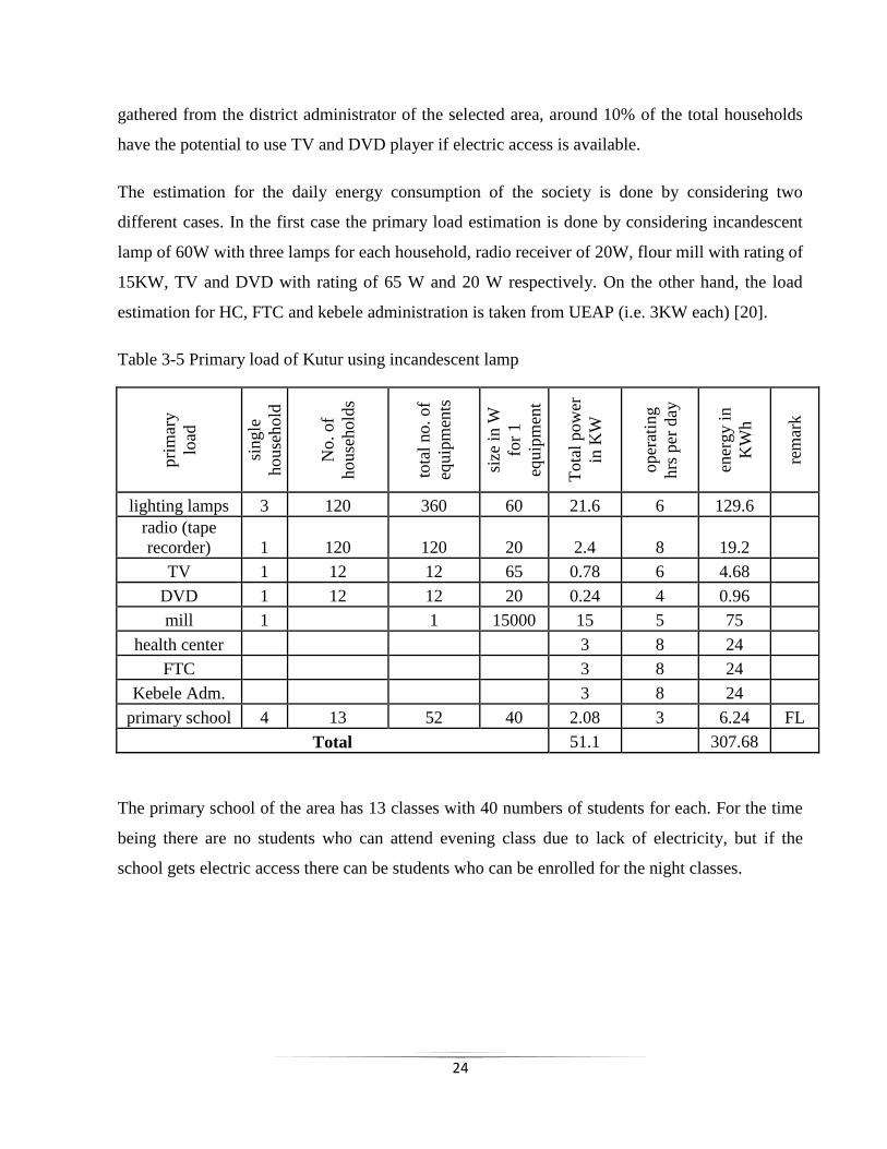
gathered from the district administrator of the selected area, around 10% of the total households
have the potential to use TV and DVD player if electric access is available.
The estimation for the daily energy consumption of the society is done by considering two
different cases. In the first case the primary load estimation is done by considering incandescent
lamp of 60W with three lamps for each household, radio receiver of 20W, flour mill with rating of
15KW, TV and DVD with rating of 65 W and 20 W respectively. On the other hand, the load
estimation for HC, FTC and kebele administration is taken from UEAP (i.e. 3KW each) [20].
Table 3-5 Primary load of Kutur using incandescent lamp
pri
mar
y
load
single
house
hold
No. of
house
hold
s
tota
l no. of
equip
men
ts
size
in W
for
1
equip
men
t
Tota
l pow
er
in K
W
oper
atin
g
hrs
per
day
ener
gy i
n
KW
h
rem
ark
lighting lamps 3 120 360 60 21.6 6 129.6
radio (tape
recorder) 1 120 120 20 2.4 8 19.2
TV 1 12 12 65 0.78 6 4.68
DVD 1 12 12 20 0.24 4 0.96
mill 1 1 15000 15 5 75
health center 3 8 24
FTC 3 8 24
Kebele Adm. 3 8 24
primary school 4 13 52 40 2.08 3 6.24 FL
Total 51.1 307.68
The primary school of the area has 13 classes with 40 numbers of students for each. For the time
being there are no students who can attend evening class due to lack of electricity, but if the
school gets electric access there can be students who can be enrolled for the night classes.
25
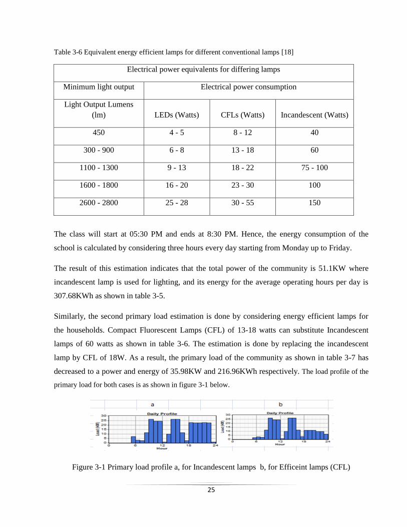
Table 3-6 Equivalent energy efficient lamps for different conventional lamps [18]
Electrical power equivalents for differing lamps
Minimum light output Electrical power consumption
Light Output Lumens
(lm) LEDs (Watts) CFLs (Watts) Incandescent (Watts)
450 4 - 5 8 - 12 40
300 - 900 6 - 8 13 - 18 60
1100 - 1300 9 - 13 18 - 22 75 - 100
1600 - 1800 16 - 20 23 - 30 100
2600 - 2800 25 - 28 30 - 55 150
The class will start at 05:30 PM and ends at 8:30 PM. Hence, the energy consumption of the
school is calculated by considering three hours every day starting from Monday up to Friday.
The result of this estimation indicates that the total power of the community is 51.1KW where
incandescent lamp is used for lighting, and its energy for the average operating hours per day is
307.68KWh as shown in table 3-5.
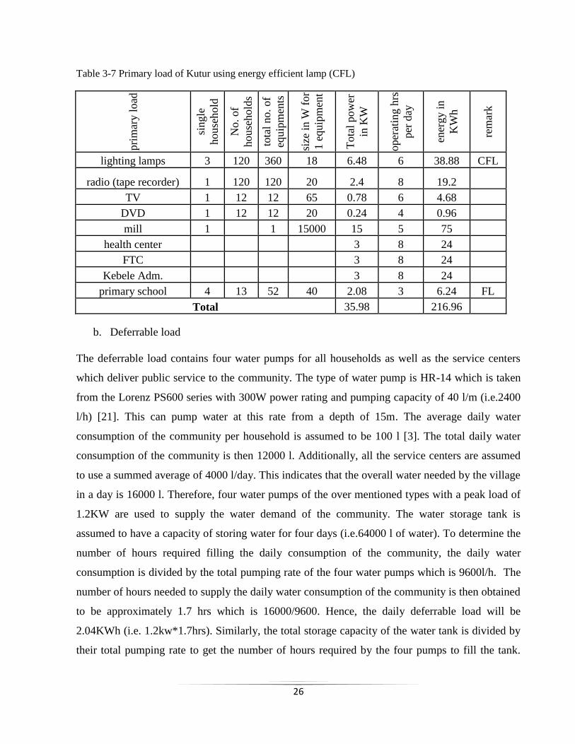
Similarly, the second primary load estimation is done by considering energy efficient lamps for
the households. Compact Fluorescent Lamps (CFL) of 13-18 watts can substitute Incandescent
lamps of 60 watts as shown in table 3-6. The estimation is done by replacing the incandescent
lamp by CFL of 18W. As a result, the primary load of the community as shown in table 3-7 has
decreased to a power and energy of 35.98KW and 216.96KWh respectively. The load profile of the
primary load for both cases is as shown in figure 3-1 below.
Figure 3-1 Primary load profile a, for Incandescent lamps b, for Efficeint lamps (CFL)
26
Table 3-7 Primary load of Kutur using energy efficient lamp (CFL)
pri
mar
y l
oad
single
house
hold
No. of
house
hold
s
tota
l no. of
equip
men
ts
size
in W
for
1 e
quip
men
t
Tota
l pow
er
in K
W
oper
atin
g h
rs
per
day
ener
gy i
n
KW
h
rem
ark
lighting lamps 3 120 360 18 6.48 6 38.88 CFL
radio (tape recorder) 1 120 120 20 2.4 8 19.2
TV 1 12 12 65 0.78 6 4.68
DVD 1 12 12 20 0.24 4 0.96
mill 1 1 15000 15 5 75
health center 3 8 24
FTC 3 8 24
Kebele Adm. 3 8 24
primary school 4 13 52 40 2.08 3 6.24 FL
Total 35.98 216.96
b. Deferrable load
The deferrable load contains four water pumps for all households as well as the service centers
which deliver public service to the community. The type of water pump is HR-14 which is taken
from the Lorenz PS600 series with 300W power rating and pumping capacity of 40 l/m (i.e.2400
l/h) [21]. This can pump water at this rate from a depth of 15m. The average daily water
consumption of the community per household is assumed to be 100 l [3]. The total daily water
consumption of the community is then 12000 l. Additionally, all the service centers are assumed
to use a summed average of 4000 l/day. This indicates that the overall water needed by the village
in a day is 16000 l. Therefore, four water pumps of the over mentioned types with a peak load of
1.2KW are used to supply the water demand of the community. The water storage tank is
assumed to have a capacity of storing water for four days (i.e.64000 l of water). To determine the
number of hours required filling the daily consumption of the community, the daily water
consumption is divided by the total pumping rate of the four water pumps which is 9600l/h. The
number of hours needed to supply the daily water consumption of the community is then obtained
to be approximately 1.7 hrs which is 16000/9600. Hence, the daily deferrable load will be
2.04KWh (i.e. 1.2kw*1.7hrs). Similarly, the total storage capacity of the water tank is divided by
their total pumping rate to get the number of hours required by the four pumps to fill the tank.
27
And this is obtained to be 6.67hrs. This result is then multiplied with the total power demanded by
the water pumps which is 1.2kW to get the corresponding energy equivalent of the reservoir
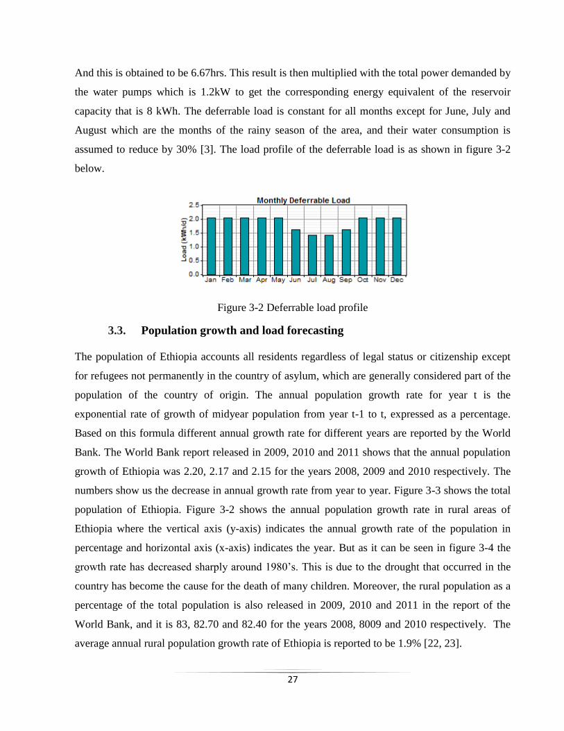
capacity that is 8 kWh. The deferrable load is constant for all months except for June, July and
August which are the months of the rainy season of the area, and their water consumption is
assumed to reduce by 30% [3]. The load profile of the deferrable load is as shown in figure 3-2
below.
Figure 3-2 Deferrable load profile
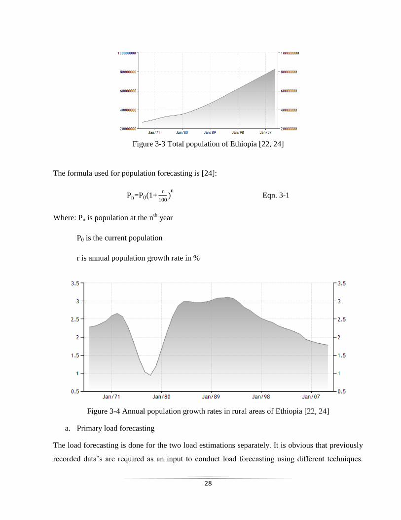
3.3. Population growth and load forecasting
The population of Ethiopia accounts all residents regardless of legal status or citizenship except
for refugees not permanently in the country of asylum, which are generally considered part of the
population of the country of origin. The annual population growth rate for year t is the
exponential rate of growth of midyear population from year t-1 to t, expressed as a percentage.
Based on this formula different annual growth rate for different years are reported by the World
Bank. The World Bank report released in 2009, 2010 and 2011 shows that the annual population
growth of Ethiopia was 2.20, 2.17 and 2.15 for the years 2008, 2009 and 2010 respectively. The
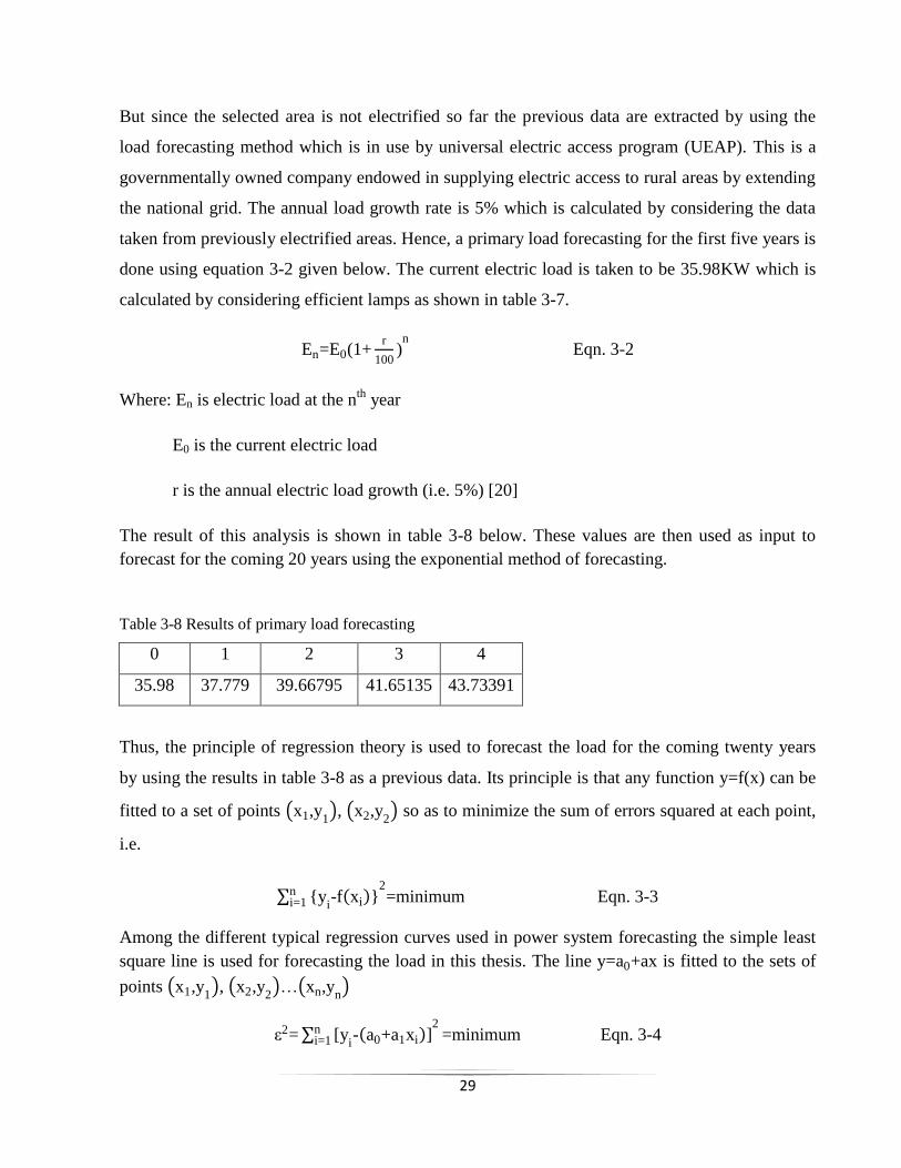
numbers show us the decrease in annual growth rate from year to year. Figure 3-3 shows the total
population of Ethiopia. Figure 3-2 shows the annual population growth rate in rural areas of
Ethiopia where the vertical axis (y-axis) indicates the annual growth rate of the population in
percentage and horizontal axis (x-axis) indicates the year. But as it can be seen in figure 3-4 the
growth rate has decreased sharply around 1980‟s. This is due to the drought that occurred in the
country has become the cause for the death of many children. Moreover, the rural population as a
percentage of the total population is also released in 2009, 2010 and 2011 in the report of the
World Bank, and it is 83, 82.70 and 82.40 for the years 2008, 8009 and 2010 respectively. The
average annual rural population growth rate of Ethiopia is reported to be 1.9% [22, 23].
28
Figure 3-3 Total population of Ethiopia [22, 24]
The formula used for population forecasting is [24]:
Pn=P0(1+r
100)n Eqn. 3-1
Where: Pn is population at the nth
year
P0 is the current population
r is annual population growth rate in %
Figure 3-4 Annual population growth rates in rural areas of Ethiopia [22, 24]
a. Primary load forecasting
The load forecasting is done for the two load estimations separately. It is obvious that previously
recorded data‟s are required as an input to conduct load forecasting using different techniques.
29
But since the selected area is not electrified so far the previous data are extracted by using the
load forecasting method which is in use by universal electric access program (UEAP). This is a
governmentally owned company endowed in supplying electric access to rural areas by extending
the national grid. The annual load growth rate is 5% which is calculated by considering the data
taken from previously electrified areas. Hence, a primary load forecasting for the first five years is
done using equation 3-2 given below. The current electric load is taken to be 35.98KW which is
calculated by considering efficient lamps as shown in table 3-7.
En=E0(1+r
100)n Eqn. 3-2
Where: En is electric load at the nth
year
E0 is the current electric load
r is the annual electric load growth (i.e. 5%) [20]
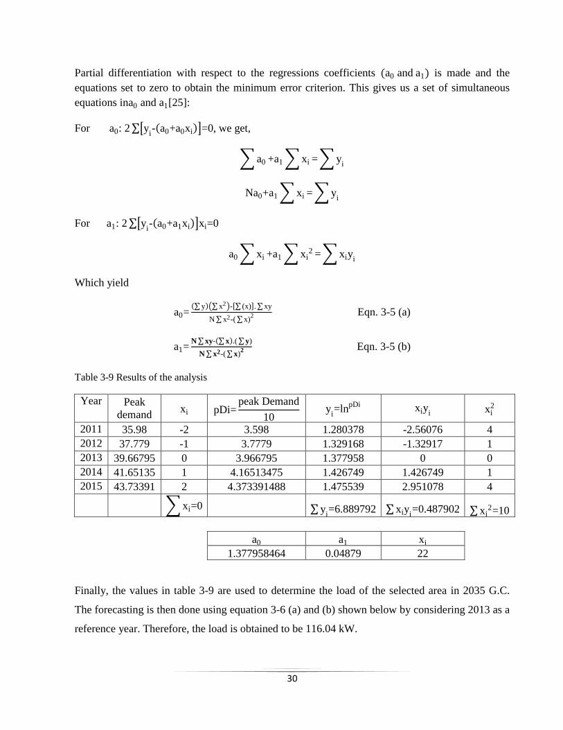
The result of this analysis is shown in table 3-8 below. These values are then used as input to
forecast for the coming 20 years using the exponential method of forecasting.
Table 3-8 Results of primary load forecasting
0 1 2 3 4
35.98 37.779 39.66795 41.65135 43.73391
Thus, the principle of regression theory is used to forecast the load for the coming twenty years
by using the results in table 3-8 as a previous data. Its principle is that any function y=f(x) can be
fitted to a set of points x1,y1 , x2,y
2 so as to minimize the sum of errors squared at each point,
i.e.
{yi-f xi }
2=minimumn
i=1 Eqn. 3-3
Among the different typical regression curves used in power system forecasting the simple least
square line is used for forecasting the load in this thesis. The line y=a0+ax is fitted to the sets of
points x1,y1 , x2,y
2 … xn,y
n
ε2= [yi- a0+a1xi ]
2ni=1 =minimum Eqn. 3-4
30
Partial differentiation with respect to the regressions coefficients (a0 and a1) is made and the
equations set to zero to obtain the minimum error criterion. This gives us a set of simultaneous
equations ina0 and a1[25]:
For a0: 2 yi- a0+a0xi =0, we get,
a0 +a1 xi = yi
Na0+a1 xi = yi
For a1: 2 yi- a0+a1xi xi=0
a0 xi +a1 xi2 = xiyi
Which yield
a0= y x2 - (x) . xy
N x2-( x)2 Eqn. 3-5 (a)
a1=N xy- x .( y)
N x2-( x)2 Eqn. 3-5 (b)
Table 3-9 Results of the analysis
Year Peak
demand xi pDi=
peak Demand
10 y
i=ln
pDi xiyi
xi2
2011 35.98 -2 3.598 1.280378 -2.56076 4
2012 37.779 -1 3.7779 1.329168 -1.32917 1
2013 39.66795 0 3.966795 1.377958 0 0
2014 41.65135 1 4.16513475 1.426749 1.426749 1
2015 43.73391 2 4.373391488 1.475539 2.951078 4
xi=0 y
i=6.889792 xiyi
=0.487902 xi2=10
a0 a1 xi
1.377958464 0.04879 22
Finally, the values in table 3-9 are used to determine the load of the selected area in 2035 G.C.
The forecasting is then done using equation 3-6 (a) and (b) shown below by considering 2013 as a
reference year. Therefore, the load is obtained to be 116.04 kW.
31
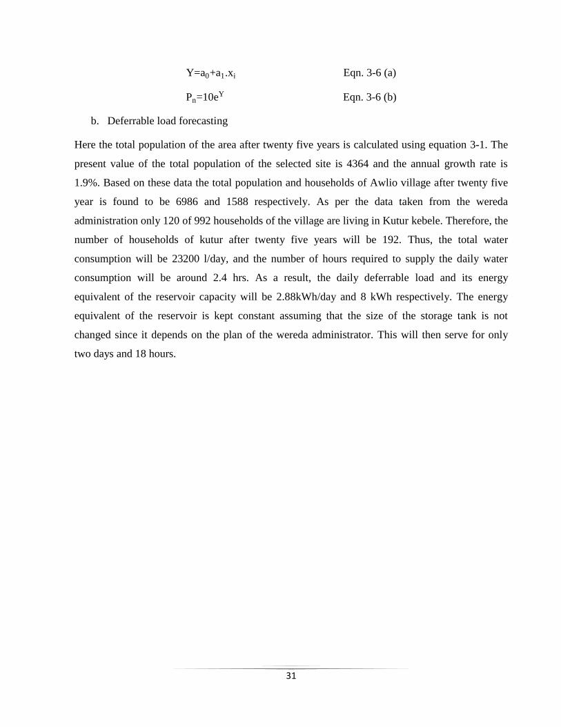
Y=a0+a1.xi Eqn. 3-6 (a)
Pn=10eY Eqn. 3-6 (b)
b. Deferrable load forecasting
Here the total population of the area after twenty five years is calculated using equation 3-1. The
present value of the total population of the selected site is 4364 and the annual growth rate is
1.9%. Based on these data the total population and households of Awlio village after twenty five
year is found to be 6986 and 1588 respectively. As per the data taken from the wereda
administration only 120 of 992 households of the village are living in Kutur kebele. Therefore, the
number of households of kutur after twenty five years will be 192. Thus, the total water
consumption will be 23200 l/day, and the number of hours required to supply the daily water
consumption will be around 2.4 hrs. As a result, the daily deferrable load and its energy
equivalent of the reservoir capacity will be 2.88kWh/day and 8 kWh respectively. The energy
equivalent of the reservoir is kept constant assuming that the size of the storage tank is not
changed since it depends on the plan of the wereda administrator. This will then serve for only
two days and 18 hours.
32
4. Modeling of the hybrid system and cost analysis of grid extension
4.1. Modeling the hybrid system
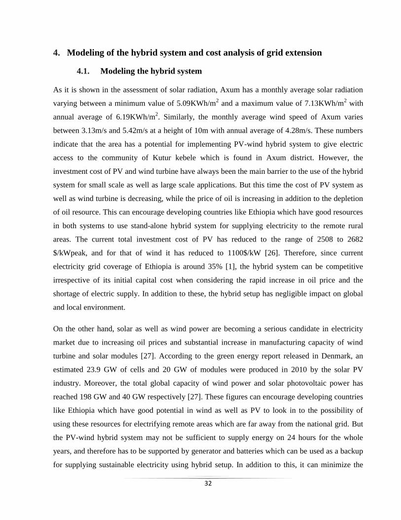
As it is shown in the assessment of solar radiation, Axum has a monthly average solar radiation
varying between a minimum value of 5.09KWh/m2 and a maximum value of 7.13KWh/m
2 with
annual average of 6.19KWh/m2. Similarly, the monthly average wind speed of Axum varies
between 3.13m/s and 5.42m/s at a height of 10m with annual average of 4.28m/s. These numbers
indicate that the area has a potential for implementing PV-wind hybrid system to give electric
access to the community of Kutur kebele which is found in Axum district. However, the
investment cost of PV and wind turbine have always been the main barrier to the use of the hybrid
system for small scale as well as large scale applications. But this time the cost of PV system as
well as wind turbine is decreasing, while the price of oil is increasing in addition to the depletion
of oil resource. This can encourage developing countries like Ethiopia which have good resources
in both systems to use stand-alone hybrid system for supplying electricity to the remote rural
areas. The current total investment cost of PV has reduced to the range of 2508 to 2682
$/kWpeak, and for that of wind it has reduced to 1100$/kW [26]. Therefore, since current
electricity grid coverage of Ethiopia is around 35% [1], the hybrid system can be competitive
irrespective of its initial capital cost when considering the rapid increase in oil price and the
shortage of electric supply. In addition to these, the hybrid setup has negligible impact on global
and local environment.
On the other hand, solar as well as wind power are becoming a serious candidate in electricity
market due to increasing oil prices and substantial increase in manufacturing capacity of wind
turbine and solar modules [27]. According to the green energy report released in Denmark, an
estimated 23.9 GW of cells and 20 GW of modules were produced in 2010 by the solar PV
industry. Moreover, the total global capacity of wind power and solar photovoltaic power has
reached 198 GW and 40 GW respectively [27]. These figures can encourage developing countries
like Ethiopia which have good potential in wind as well as PV to look in to the possibility of
using these resources for electrifying remote areas which are far away from the national grid. But
the PV-wind hybrid system may not be sufficient to supply energy on 24 hours for the whole
years, and therefore has to be supported by generator and batteries which can be used as a backup
for supplying sustainable electricity using hybrid setup. In addition to this, it can minimize the
33
investment cost of the setup since the cost of generators varies between 200 $/kW and 228 $/kW
[21, 28].
The main objective of this work is to assess resource potential and to model PV-Wind hybrid
system with generator and battery as a back up to electrify 120 households of Kutur kebele, and
the model is also simulated for the load at the end of the life span of the project which is obtained
using simple load forecasting. Additionally, it will compare the initial capital cost of the hybrid
system against the cost required for extending a grid.
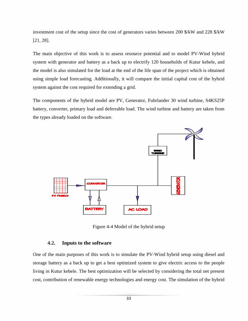
The components of the hybrid model are PV, Generator, Fuhrlander 30 wind turbine, S4KS25P
battery, converter, primary load and deferrable load. The wind turbine and battery are taken from
the types already loaded on the software.
Figure 4-4 Model of the hybrid setup
4.2. Inputs to the software
One of the main purposes of this work is to simulate the PV-Wind hybrid setup using diesel and
storage battery as a back up to get a best optimized system to give electric access to the people
living in Kutur kebele. The best optimization will be selected by considering the total net present
cost, contribution of renewable energy technologies and energy cost. The simulation of the hybrid
34
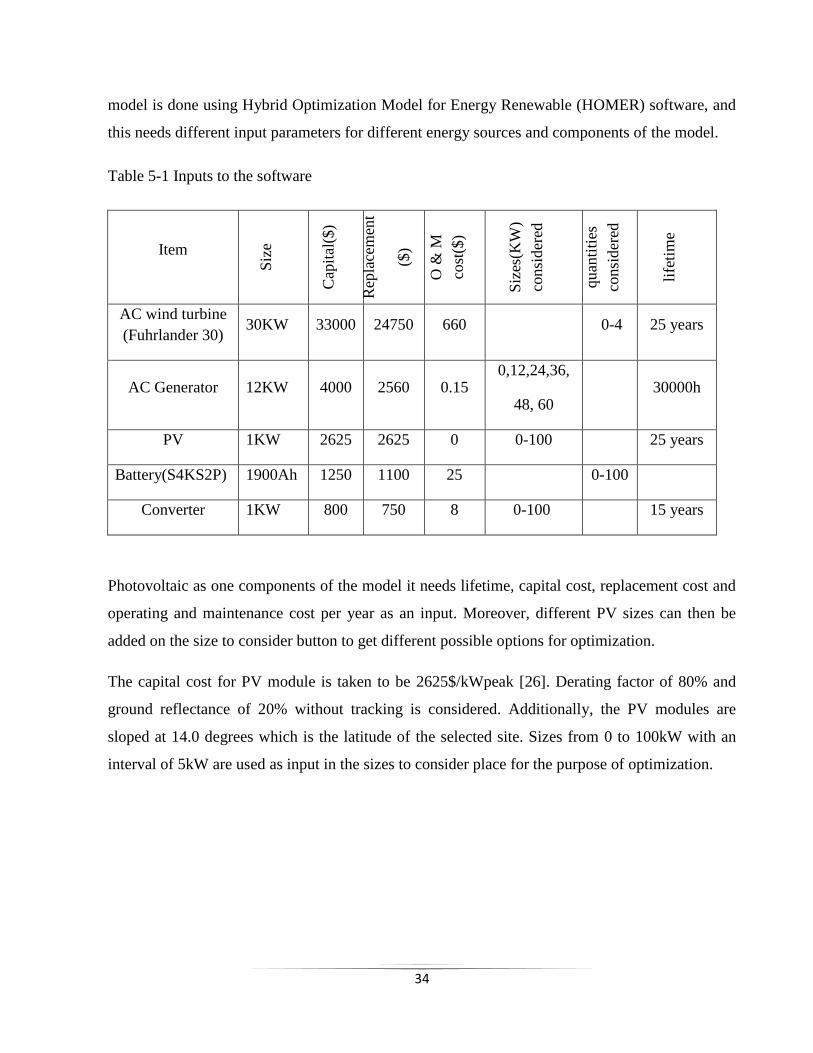
model is done using Hybrid Optimization Model for Energy Renewable (HOMER) software, and
this needs different input parameters for different energy sources and components of the model.
Table 5-1 Inputs to the software
Item S
ize
Cap
ital
($)
Rep
lace
men
t
($)
O &
M
cost
($)
Siz
es(K
W)
consi
der
ed
quan
titi
es
consi
der
ed
life
tim
e
AC wind turbine
(Fuhrlander 30) 30KW 33000 24750 660
0-4 25 years
AC Generator 12KW 4000 2560 0.15 0,12,24,36,
48, 60 30000h
PV 1KW 2625 2625 0 0-100 25 years
Battery(S4KS2P) 1900Ah 1250 1100 25 0-100
Converter 1KW 800 750 8 0-100
15 years
Photovoltaic as one components of the model it needs lifetime, capital cost, replacement cost and
operating and maintenance cost per year as an input. Moreover, different PV sizes can then be
added on the size to consider button to get different possible options for optimization.
The capital cost for PV module is taken to be 2625$/kWpeak [26]. Derating factor of 80% and
ground reflectance of 20% without tracking is considered. Additionally, the PV modules are
sloped at 14.0 degrees which is the latitude of the selected site. Sizes from 0 to 100kW with an
interval of 5kW are used as input in the sizes to consider place for the purpose of optimization.
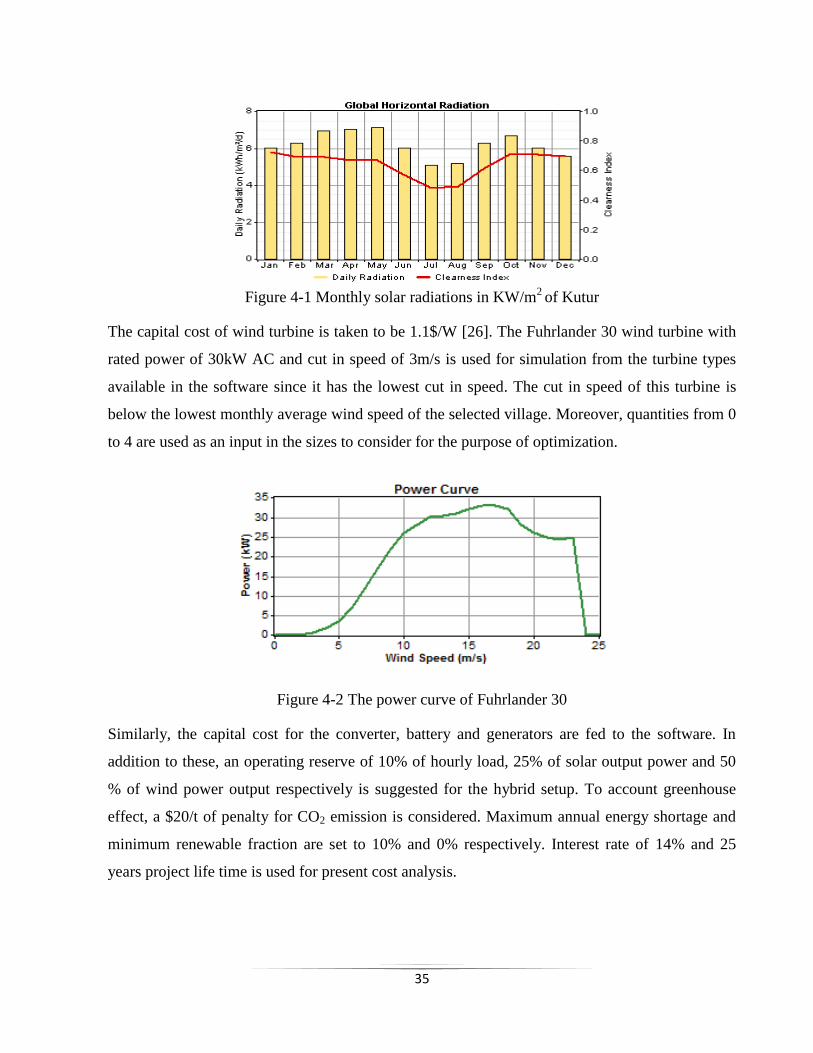
35
Figure 4-1 Monthly solar radiations in KW/m
2 of Kutur
The capital cost of wind turbine is taken to be 1.1$/W [26]. The Fuhrlander 30 wind turbine with
rated power of 30kW AC and cut in speed of 3m/s is used for simulation from the turbine types
available in the software since it has the lowest cut in speed. The cut in speed of this turbine is
below the lowest monthly average wind speed of the selected village. Moreover, quantities from 0
to 4 are used as an input in the sizes to consider for the purpose of optimization.
Figure 4-2 The power curve of Fuhrlander 30
Similarly, the capital cost for the converter, battery and generators are fed to the software. In
addition to these, an operating reserve of 10% of hourly load, 25% of solar output power and 50
% of wind power output respectively is suggested for the hybrid setup. To account greenhouse
effect, a $20/t of penalty for CO2 emission is considered. Maximum annual energy shortage and
minimum renewable fraction are set to 10% and 0% respectively. Interest rate of 14% and 25
years project life time is used for present cost analysis.
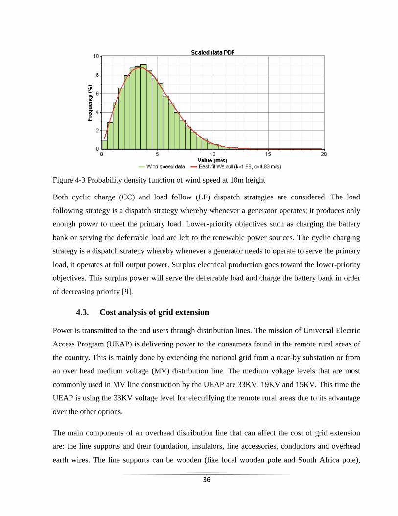
36
Figure 4-3 Probability density function of wind speed at 10m height
Both cyclic charge (CC) and load follow (LF) dispatch strategies are considered. The load
following strategy is a dispatch strategy whereby whenever a generator operates; it produces only
enough power to meet the primary load. Lower-priority objectives such as charging the battery
bank or serving the deferrable load are left to the renewable power sources. The cyclic charging
strategy is a dispatch strategy whereby whenever a generator needs to operate to serve the primary
load, it operates at full output power. Surplus electrical production goes toward the lower-priority
objectives. This surplus power will serve the deferrable load and charge the battery bank in order
of decreasing priority [9].
4.3. Cost analysis of grid extension
Power is transmitted to the end users through distribution lines. The mission of Universal Electric
Access Program (UEAP) is delivering power to the consumers found in the remote rural areas of
the country. This is mainly done by extending the national grid from a near-by substation or from
an over head medium voltage (MV) distribution line. The medium voltage levels that are most
commonly used in MV line construction by the UEAP are 33KV, 19KV and 15KV. This time the
UEAP is using the 33KV voltage level for electrifying the remote rural areas due to its advantage
over the other options.
The main components of an overhead distribution line that can affect the cost of grid extension
are: the line supports and their foundation, insulators, line accessories, conductors and overhead
earth wires. The line supports can be wooden (like local wooden pole and South Africa pole),

37
reinforced concrete pole and steel, but due to its strength and availability UEAP is using concrete
poles for MV distribution line to give electric access for the people of rural areas.
The main tasks during line extension are surveying, excavation, pole erection, pole top
configuration and stringing of conductors. For the MV distribution line construction All
Aluminum Alloy Conductor with a size of 95mm2 and 50mm
2 are used. However, the number of
poles to be erected and the requirement of angle assemblies depend on the distance of the site
from a nearby substation or MV distribution line, and geographical location of the selected site.
Moreover, different accessories are used depending on type of assemblies. The assemblies that
can be used in the construction are suspension, light angle 1, light angle 2, heavy angle, T-off,
tension tower, and dead-end. These are classified based on the angle deviation from a straight line
[20].
Based on the note mentioned earlier, the cost estimation for delivering electric access to Kutur
village which is found in Axum is done. The distance of Kutur from an existing grid (i.e. Axum)
is 30km, and based on this distance a rough survey is conducted to select the best route, and to
identify the type of assemblies to be used for MV distribution line construction during the site
visit. The power demand of the community and the rating of the transformers are estimated by the
standard Excel sheet the UEAP is using now. As a result, the number of transformers needed for
the community is obtained to be 1x50KVA and 1x100KVA.
Therefore, to give electric access to the 120 households, HC, FTC, flour mill, kebele
administration and primary school of Kutur from the national grid found nearby, it needs
extension of 30 km MV line and erection of two transformers with a rating of 1x50KVA and
1x100KVA. Hence, the cost is analyzed using an interlinked spread Microsoft excel sheet used by
the UEAP; and the result obtained is as shown in table 4-1. The total cost includes material,
transportation and labor cost. The investment cost is therefore obtained to be 5,007,181.05
Ethiopian birr which is equivalent with 285,309.5 US dollar.
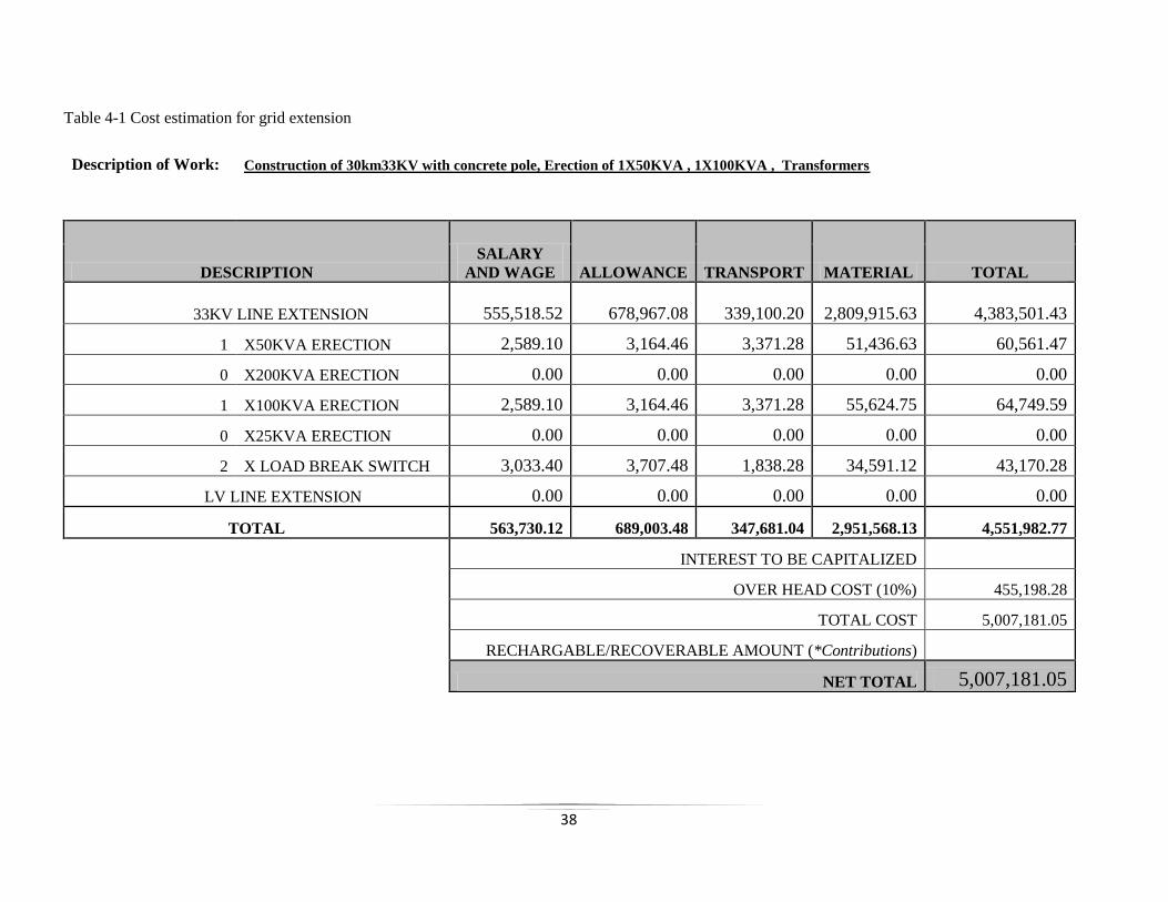
38
Table 4-1 Cost estimation for grid extension
Description of Work: Construction of 30km33KV with concrete pole, Erection of 1X50KVA , 1X100KVA , Transformers
DESCRIPTION
SALARY
AND WAGE ALLOWANCE TRANSPORT MATERIAL TOTAL
33KV LINE EXTENSION 555,518.52 678,967.08 339,100.20
2,809,915.63 4,383,501.43
1 X50KVA ERECTION 2,589.10 3,164.46 3,371.28 51,436.63 60,561.47
0 X200KVA ERECTION 0.00 0.00 0.00 0.00 0.00
1 X100KVA ERECTION 2,589.10 3,164.46 3,371.28 55,624.75 64,749.59
0 X25KVA ERECTION 0.00 0.00 0.00 0.00 0.00
2 X LOAD BREAK SWITCH 3,033.40 3,707.48 1,838.28 34,591.12 43,170.28
LV LINE EXTENSION 0.00 0.00 0.00 0.00 0.00
TOTAL 563,730.12 689,003.48 347,681.04 2,951,568.13 4,551,982.77
INTEREST TO BE CAPITALIZED
OVER HEAD COST (10%) 455,198.28
TOTAL COST 5,007,181.05
RECHARGABLE/RECOVERABLE AMOUNT (*Contributions)
NET TOTAL 5,007,181.05
39
5. Results, Discussion and Conclusion
5.1. Results of the simulation
The simulation result window of HOMER displays the components of the system and three
outputs (i.e. the total net present cost, levelized cost of energy, and operating cost). In addition,
the window has cost summary tab which displays the total cash flow, categorized either by
component or by cost type, and electrical tab which displays details about the production and
consumption of electricity by the system. The other tabs are PV, wind turbine, generator, grid,
battery, converter and emissions.
HOMER simulates every system in the search space and ranks all feasible systems according to
increasing net present cost, and displays the result in the optimization tab. The list of the
optimization results which are capable of meeting the system load and constraints are then
displayed in overall form and categorized form. In the overall form the top ranked system
configuration (i.e. a combination of a particular numbers and size of components) according to
the net present cost (NPC) are displayed. However, in the categorized form only the least-cost
systems for each system configuration are displayed.
In the optimization result it can be observed, size of different components in each system
configuration and their symbols, dispatch strategy, initial capital, operating and maintenance
cost, total NPC, COE, renewable fraction and shortage capacity. Moreover, the consumption of
diesel and operating hours of the generators can also be easily observed.
A sensitivity analysis is also done to get an answer for the effect of input variables having
dynamic nature. It takes the most cost effective system configuration for each combination of
sensitive variable values. The results of this analysis can be displayed either in a graphic or
tabular form. In this work PV capital cost multiplier linked with PV replacement cost
multiplier, wind speed and diesel price are used as sensitivity parameters for sensitivity
analysis, even though, there are a lot of parameters to be considered.
Therefore, HOMER is used for simulating the hybrid system containing PV, wind, converter,
diesel and storage battery. To get optimal combination of the hybrid components which could
be implemented as a hybrid system for supplying electricity to the community of Kutur kebele,
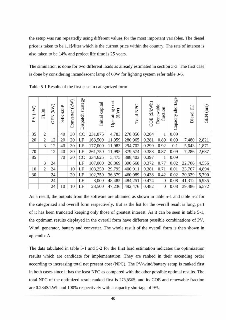
40
the setup was run repeatedly using different values for the most important variables. The diesel
price is taken to be 1.1$/liter which is the current price within the country. The rate of interest is
also taken to be 14% and project life time is 25 years.
The simulation is done for two different loads as already estimated in section 3-3. The first case
is done by considering incandescent lamp of 60W for lighting system refer table 3-6.
Table 5-1 Results of the first case in categorized form
PV
(kW
)
FL
30
GE
N (
kW
)
S4K
S25P
Conver
ter
(kW
)
Dis
pat
ch s
trat
egy
Init
ial
capit
al
Oper
atin
g c
ost
($/y
r)
Tota
l N
PC
CO
E (
$/k
Wh)
Ren
ewab
le
frac
tion
Cap
acit
y s
hort
age
Die
sel
(L)
GE
N (
hrs
)
35 2 40 30 CC 231,875 4,783 278,856 0.284 1 0.09
20 2 12 20 20 LF 163,500 11,959 280,965 0.281 0.89 0.09 7,480 2,821
3 12 40 30 LF 177,000 11,983 294,702 0.299 0.92 0.1 5,643 1,871
70 12 40 30 LF 261,750 11,995 379,574 0.388 0.87 0.09 7,286 2,687
85 70 30 CC 334,625 5,475 388,403 0.397 1 0.09
3 24 LF 107,000 28,869 390,568 0.372 0.77 0.02 22,706 4,556
10 2 24 10 LF 108,250 29,795 400,911 0.381 0.71 0.01 23,767 4,894
30 24 20 LF 102,750 36,379 460,089 0.438 0.42 0.02 30,329 5,790
24 LF 8,000 48,485 484,251 0.474 0 0.08 41,312 6,935
24 10 10 LF 28,500 47,236 492,476 0.482 0 0.08 39,486 6,572
As a result, the outputs from the software are obtained as shown in table 5-1 and table 5-2 for
the categorized and overall form respectively. But as the list for the overall result is long, part
of it has been truncated keeping only those of greatest interest. As it can be seen in table 5-1,
the optimum results displayed in the overall form have different possible combinations of PV,
Wind, generator, battery and converter. The whole result of the overall form is then shown in
appendix A.
The data tabulated in table 5-1 and 5-2 for the first load estimation indicates the optimization
results which are candidate for implementation. They are ranked in their ascending order
according to increasing total net present cost (NPC). The PV/wind/battery setup is ranked first
in both cases since it has the least NPC as compared with the other possible optimal results. The
total NPC of the optimized result ranked first is 278,856$, and its COE and renewable fraction
are 0.284$/kWh and 100% respectively with a capacity shortage of 9%.
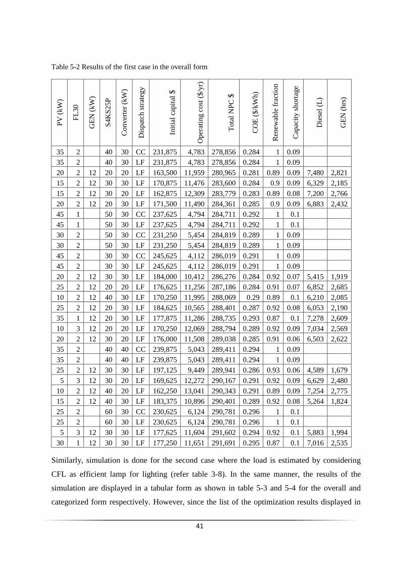
41
Table 5-2 Results of the first case in the overall form P
V (
kW
)
FL
30
GE
N (
kW
)
S4
KS
25
P
Co
nv
erte
r (k
W)
Dis
pat
ch s
trat
egy
Init
ial
cap
ital
$
Op
erat
ing c
ost
($
/yr)
To
tal
NP
C $
CO
E (
$/k
Wh
)
Ren
ewab
le f
ract
ion
Cap
acit
y s
ho
rtag
e
Die
sel
(L)
GE
N (
hrs
)
35 2 40 30 CC 231,875 4,783 278,856 0.284 1 0.09
35 2 40 30 LF 231,875 4,783 278,856 0.284 1 0.09
20 2 12 20 20 LF 163,500 11,959 280,965 0.281 0.89 0.09 7,480 2,821
15 2 12 30 30 LF 170,875 11,476 283,600 0.284 0.9 0.09 6,329 2,185
15 2 12 30 20 LF 162,875 12,309 283,779 0.283 0.89 0.08 7,200 2,766
20 2 12 20 30 LF 171,500 11,490 284,361 0.285 0.9 0.09 6,883 2,432
45 1 50 30 CC 237,625 4,794 284,711 0.292 1 0.1
45 1 50 30 LF 237,625 4,794 284,711 0.292 1 0.1
30 2 50 30 CC 231,250 5,454 284,819 0.289 1 0.09
30 2 50 30 LF 231,250 5,454 284,819 0.289 1 0.09
45 2 30 30 CC 245,625 4,112 286,019 0.291 1 0.09
45 2 30 30 LF 245,625 4,112 286,019 0.291 1 0.09
20 2 12 30 30 LF 184,000 10,412 286,276 0.284 0.92 0.07 5,415 1,919
25 2 12 20 20 LF 176,625 11,256 287,186 0.284 0.91 0.07 6,852 2,685
10 2 12 40 30 LF 170,250 11,995 288,069 0.29 0.89 0.1 6,210 2,085
25 2 12 20 30 LF 184,625 10,565 288,401 0.287 0.92 0.08 6,053 2,190
35 1 12 20 30 LF 177,875 11,286 288,735 0.293 0.87 0.1 7,278 2,609
10 3 12 20 20 LF 170,250 12,069 288,794 0.289 0.92 0.09 7,034 2,569
20 2 12 30 20 LF 176,000 11,508 289,038 0.285 0.91 0.06 6,503 2,622
35 2 40 40 CC 239,875 5,043 289,411 0.294 1 0.09
35 2 40 40 LF 239,875 5,043 289,411 0.294 1 0.09
25 2 12 30 30 LF 197,125 9,449 289,941 0.286 0.93 0.06 4,589 1,679
5 3 12 30 20 LF 169,625 12,272 290,167 0.291 0.92 0.09 6,629 2,480
10 2 12 40 20 LF 162,250 13,041 290,343 0.291 0.89 0.09 7,254 2,775
15 2 12 40 30 LF 183,375 10,896 290,401 0.289 0.92 0.08 5,264 1,824
25 2 60 30 CC 230,625 6,124 290,781 0.296 1 0.1
25 2 60 30 LF 230,625 6,124 290,781 0.296 1 0.1
5 3 12 30 30 LF 177,625 11,604 291,602 0.294 0.92 0.1 5,883 1,994
30 1 12 30 30 LF 177,250 11,651 291,691 0.295 0.87 0.1 7,016 2,535
Similarly, simulation is done for the second case where the load is estimated by considering
CFL as efficient lamp for lighting (refer table 3-8). In the same manner, the results of the
simulation are displayed in a tabular form as shown in table 5-3 and 5-4 for the overall and
categorized form respectively. However, since the list of the optimization results displayed in
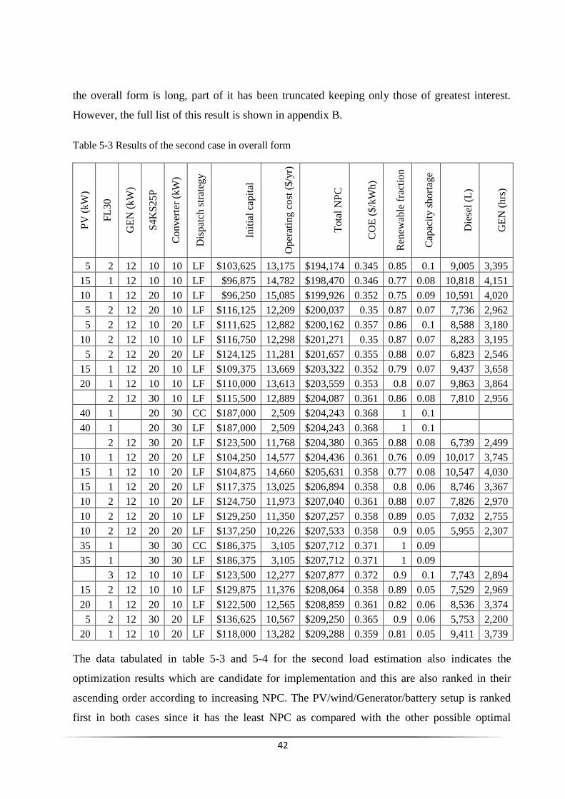
42
the overall form is long, part of it has been truncated keeping only those of greatest interest.
However, the full list of this result is shown in appendix B.
Table 5-3 Results of the second case in overall form
PV
(k
W)
FL
30
GE
N (
kW
)
S4
KS
25
P
Co
nv
erte
r (k
W)
Dis
pat
ch s
trat
egy
Init
ial
cap
ital
Op
erat
ing c
ost
($
/yr)
To
tal
NP
C
CO
E (
$/k
Wh
)
Ren
ewab
le f
ract
ion
Cap
acit
y s
ho
rtag
e
Die
sel
(L)
GE
N (
hrs
)
5 2 12 10 10 LF $103,625 13,175 $194,174 0.345 0.85 0.1 9,005 3,395
15 1 12 10 10 LF $96,875 14,782 $198,470 0.346 0.77 0.08 10,818 4,151
10 1 12 20 10 LF $96,250 15,085 $199,926 0.352 0.75 0.09 10,591 4,020
5 2 12 20 10 LF $116,125 12,209 $200,037 0.35 0.87 0.07 7,736 2,962
5 2 12 10 20 LF $111,625 12,882 $200,162 0.357 0.86 0.1 8,588 3,180
10 2 12 10 10 LF $116,750 12,298 $201,271 0.35 0.87 0.07 8,283 3,195
5 2 12 20 20 LF $124,125 11,281 $201,657 0.355 0.88 0.07 6,823 2,546
15 1 12 20 10 LF $109,375 13,669 $203,322 0.352 0.79 0.07 9,437 3,658
20 1 12 10 10 LF $110,000 13,613 $203,559 0.353 0.8 0.07 9,863 3,864
2 12 30 10 LF $115,500 12,889 $204,087 0.361 0.86 0.08 7,810 2,956
40 1 20 30 CC $187,000 2,509 $204,243 0.368 1 0.1
40 1 20 30 LF $187,000 2,509 $204,243 0.368 1 0.1
2 12 30 20 LF $123,500 11,768 $204,380 0.365 0.88 0.08 6,739 2,499
10 1 12 20 20 LF $104,250 14,577 $204,436 0.361 0.76 0.09 10,017 3,745
15 1 12 10 20 LF $104,875 14,660 $205,631 0.358 0.77 0.08 10,547 4,030
15 1 12 20 20 LF $117,375 13,025 $206,894 0.358 0.8 0.06 8,746 3,367
10 2 12 10 20 LF $124,750 11,973 $207,040 0.361 0.88 0.07 7,826 2,970
10 2 12 20 10 LF $129,250 11,350 $207,257 0.358 0.89 0.05 7,032 2,755
10 2 12 20 20 LF $137,250 10,226 $207,533 0.358 0.9 0.05 5,955 2,307
35 1 30 30 CC $186,375 3,105 $207,712 0.371 1 0.09
35 1 30 30 LF $186,375 3,105 $207,712 0.371 1 0.09
3 12 10 10 LF $123,500 12,277 $207,877 0.372 0.9 0.1 7,743 2,894
15 2 12 10 10 LF $129,875 11,376 $208,064 0.358 0.89 0.05 7,529 2,969
20 1 12 20 10 LF $122,500 12,565 $208,859 0.361 0.82 0.06 8,536 3,374
5 2 12 30 20 LF $136,625 10,567 $209,250 0.365 0.9 0.06 5,753 2,200
20 1 12 10 20 LF $118,000 13,282 $209,288 0.359 0.81 0.05 9,411 3,739
The data tabulated in table 5-3 and 5-4 for the second load estimation also indicates the
optimization results which are candidate for implementation and this are also ranked in their
ascending order according to increasing NPC. The PV/wind/Generator/battery setup is ranked
first in both cases since it has the least NPC as compared with the other possible optimal
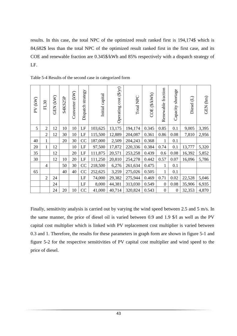
43
results. In this case, the total NPC of the optimized result ranked first is 194,174$ which is
84,682$ less than the total NPC of the optimized result ranked first in the first case, and its
COE and renewable fraction are 0.345$/kWh and 85% respectively with a dispatch strategy of
LF.
Table 5-4 Results of the second case in categorized form
PV
(k
W)
FL
30
GE
N (
kW
)
S4
KS
25
P
Co
nv
erte
r (k
W)
Dis
pat
ch s
trat
egy
Init
ial
cap
ital
Op
erat
ing c
ost
($
/yr)
To
tal
NP
C
CO
E (
$/k
Wh
)
Ren
ewab
le f
ract
ion
Cap
acit
y s
ho
rtag
e
Die
sel
(L)
GE
N (
hrs
)
5 2 12 10 10 LF 103,625 13,175 194,174 0.345 0.85 0.1 9,005 3,395
2 12 30 10 LF 115,500 12,889 204,087 0.361 0.86 0.08 7,810 2,956
40 1 20 30 CC 187,000 2,509 204,243 0.368 1 0.1
20 1 12 10 LF 97,500 17,872 220,336 0.384 0.74 0.1 13,777 5,320
35 12 20 LF 111,875 20,571 253,258 0.439 0.6 0.08 16,392 5,852
30 12 10 20 LF 111,250 20,810 254,278 0.442 0.57 0.07 16,096 5,786
4 50 30 CC 218,500 6,276 261,634 0.475 1 0.1
65 40 40 CC 252,625 3,259 275,026 0.505 1 0.1
2 24 LF 74,000 29,382 275,944 0.469 0.71 0.02 22,528 5,046
24 LF 8,000 44,381 313,030 0.549 0 0.08 35,906 6,935
24 20 10 CC 41,000 40,714 320,824 0.543 0 0 32,353 4,870
Finally, sensitivity analysis is carried out by varying the wind speed between 2.5 and 5 m/s. In
the same manner, the price of diesel oil is varied between 0.9 and 1.9 $/l as well as the PV
capital cost multiplier which is linked with PV replacement cost multiplier is varied between
0.3 and 1. Therefore, the results for these parameters in graph form are shown in figure 5-1 and
figure 5-2 for the respective sensitivities of PV capital cost multiplier and wind speed to the
price of diesel.
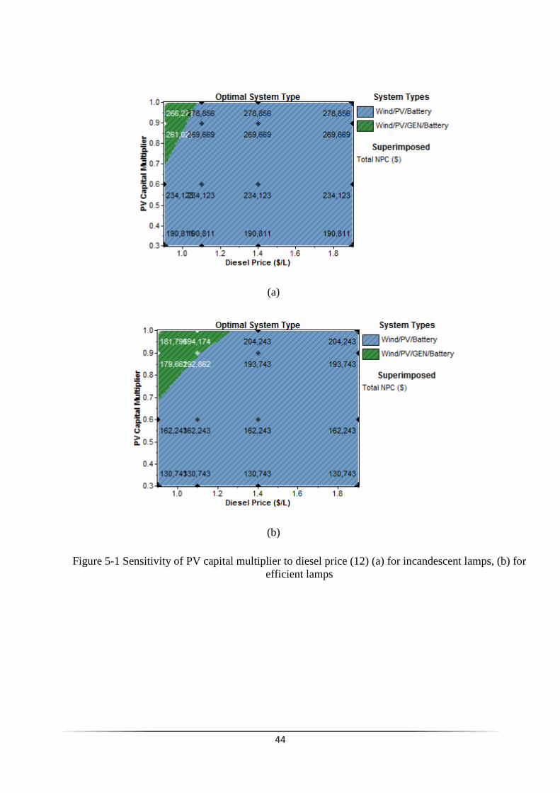
44
(a)
(b)
Figure 5-1 Sensitivity of PV capital multiplier to diesel price (12) (a) for incandescent lamps, (b) for
efficient lamps
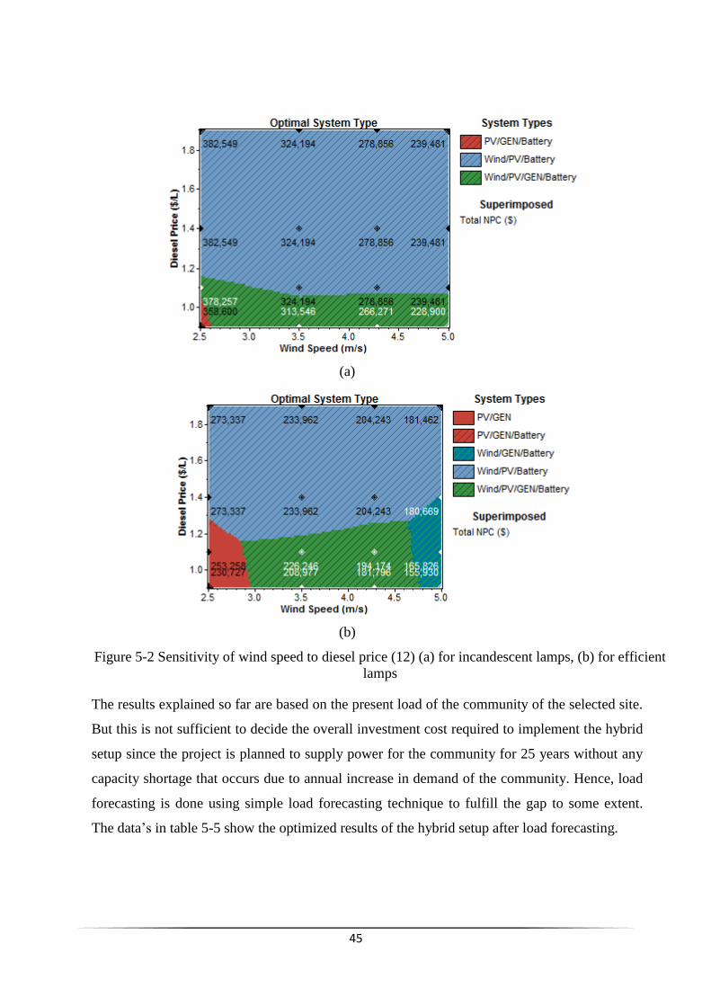
45
(a)
(b)
Figure 5-2 Sensitivity of wind speed to diesel price (12) (a) for incandescent lamps, (b) for efficient
lamps
The results explained so far are based on the present load of the community of the selected site.
But this is not sufficient to decide the overall investment cost required to implement the hybrid
setup since the project is planned to supply power for the community for 25 years without any
capacity shortage that occurs due to annual increase in demand of the community. Hence, load
forecasting is done using simple load forecasting technique to fulfill the gap to some extent.
The data‟s in table 5-5 show the optimized results of the hybrid setup after load forecasting.
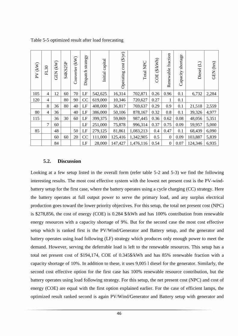
46
Table 5-5 optimized result after load forecasting P
V (
kW
)
FL
30
GE
N (
kW
)
S4
KS
25
P
Co
nv
erte
r (k
W)
Dis
pat
ch s
trat
egy
Init
ial
cap
ital
Op
erat
ing c
ost
($
/yr)
To
tal
NP
C
CO
E (
$/k
Wh
)
Ren
ewab
le f
ract
ion
Cap
acit
y s
ho
rtag
e
Die
sel
(L)
GE
N (
hrs
)
105 4 12 60 70 LF 542,625 16,314 702,871 0.26 0.96 0.1 6,732 2,284
120 4 80 90 CC 619,000 10,346 720,627 0.27 1 0.1
8 36 80 40 LF 408,000 36,817 769,637 0.29 0.9 0.1 21,518 2,559
80 4 36 40 LF 386,000 50,106 878,167 0.32 0.8 0.1 39,326 4,977
115 36 30 60 LF 399,375 59,869 987,445 0.36 0.62 0.08 48,056 5,351
7 60 LF 251,000 75,878 996,314 0.37 0.75 0.09 59,957 5,000
85 48 50 LF 279,125 81,861 1,083,213 0.4 0.47 0.1 68,439 6,090
60 60 20 CC 111,000 125,416 1,342,905 0.5 0 0.09 103,887 5,839
84 LF 28,000 147,427 1,476,116 0.54 0 0.07 124,346 6,935
5.2. Discussion
Looking at a few setup listed in the overall form (refer table 5-2 and 5-3) we find the following
interesting results. The most cost effective system with the lowest net present cost is the PV-wind-
battery setup for the first case, where the battery operates using a cycle charging (CC) strategy. Here
the battery operates at full output power to serve the primary load, and any surplus electrical
production goes toward the lower priority objectives. For this setup, the total net present cost (NPC)
is $278,856, the cost of energy (COE) is 0.284 $/kWh and has 100% contribution from renewable
energy resources with a capacity shortage of 9%. But for the second case the most cost effective
setup which is ranked first is the PV/Wind/Generator and Battery setup, and the generator and
battery operates using load following (LF) strategy which produces only enough power to meet the
demand. However, serving the deferrable load is left to the renewable resources. This setup has a
total net present cost of $194,174, COE of 0.345$/kWh and has 85% renewable fraction with a
capacity shortage of 10%. In addition to these, it uses 9,005 l diesel for the generator. Similarly, the
second cost effective option for the first case has 100% renewable resource contribution, but the
battery operates using load following strategy. For this setup, the net present cost (NPC) and cost of
energy (COE) are equal with the first option explained earlier. For the case of efficient lamps, the
optimized result ranked second is again PV/Wind/Generator and Battery setup with generator and
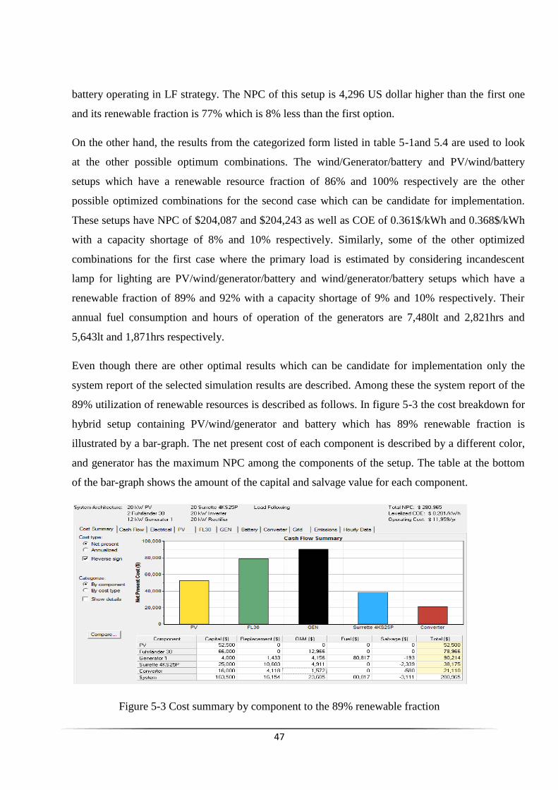
47
battery operating in LF strategy. The NPC of this setup is 4,296 US dollar higher than the first one
and its renewable fraction is 77% which is 8% less than the first option.
On the other hand, the results from the categorized form listed in table 5-1and 5.4 are used to look
at the other possible optimum combinations. The wind/Generator/battery and PV/wind/battery
setups which have a renewable resource fraction of 86% and 100% respectively are the other
possible optimized combinations for the second case which can be candidate for implementation.
These setups have NPC of $204,087 and $204,243 as well as COE of 0.361$/kWh and 0.368$/kWh
with a capacity shortage of 8% and 10% respectively. Similarly, some of the other optimized
combinations for the first case where the primary load is estimated by considering incandescent
lamp for lighting are PV/wind/generator/battery and wind/generator/battery setups which have a
renewable fraction of 89% and 92% with a capacity shortage of 9% and 10% respectively. Their
annual fuel consumption and hours of operation of the generators are 7,480lt and 2,821hrs and
5,643lt and 1,871hrs respectively.
Even though there are other optimal results which can be candidate for implementation only the
system report of the selected simulation results are described. Among these the system report of the
89% utilization of renewable resources is described as follows. In figure 5-3 the cost breakdown for
hybrid setup containing PV/wind/generator and battery which has 89% renewable fraction is
illustrated by a bar-graph. The net present cost of each component is described by a different color,
and generator has the maximum NPC among the components of the setup. The table at the bottom
of the bar-graph shows the amount of the capital and salvage value for each component.
Figure 5-3 Cost summary by component to the 89% renewable fraction
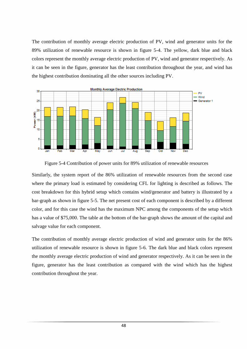
48
The contribution of monthly average electric production of PV, wind and generator units for the
89% utilization of renewable resource is shown in figure 5-4. The yellow, dark blue and black
colors represent the monthly average electric production of PV, wind and generator respectively. As
it can be seen in the figure, generator has the least contribution throughout the year, and wind has
the highest contribution dominating all the other sources including PV.
Figure 5-4 Contribution of power units for 89% utilization of renewable resources
Similarly, the system report of the 86% utilization of renewable resources from the second case
where the primary load is estimated by considering CFL for lighting is described as follows. The
cost breakdown for this hybrid setup which contains wind/generator and battery is illustrated by a
bar-graph as shown in figure 5-5. The net present cost of each component is described by a different
color, and for this case the wind has the maximum NPC among the components of the setup which
has a value of $75,000. The table at the bottom of the bar-graph shows the amount of the capital and
salvage value for each component.
The contribution of monthly average electric production of wind and generator units for the 86%
utilization of renewable resource is shown in figure 5-6. The dark blue and black colors represent
the monthly average electric production of wind and generator respectively. As it can be seen in the
figure, generator has the least contribution as compared with the wind which has the highest
contribution throughout the year.
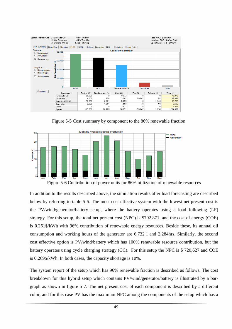
49
Figure 5-5 Cost summary by component to the 86% renewable fraction
Figure 5-6 Contribution of power units for 86% utilization of renewable resources
In addition to the results described above, the simulation results after load forecasting are described
below by referring to table 5-5. The most cost effective system with the lowest net present cost is
the PV/wind/generator/battery setup, where the battery operates using a load following (LF)
strategy. For this setup, the total net present cost (NPC) is $702,871, and the cost of energy (COE)
is 0.261$/kWh with 96% contribution of renewable energy resources. Beside these, its annual oil
consumption and working hours of the generator are 6,732 l and 2,284hrs. Similarly, the second
cost effective option is PV/wind/battery which has 100% renewable resource contribution, but the
battery operates using cycle charging strategy (CC). For this setup the NPC is $ 720,627 and COE
is 0.269$/kWh. In both cases, the capacity shortage is 10%.
The system report of the setup which has 96% renewable fraction is described as follows. The cost
breakdown for this hybrid setup which contains PV/wind/generator/battery is illustrated by a bar-
graph as shown in figure 5-7. The net present cost of each component is described by a different
color, and for this case PV has the maximum NPC among the components of the setup which has a
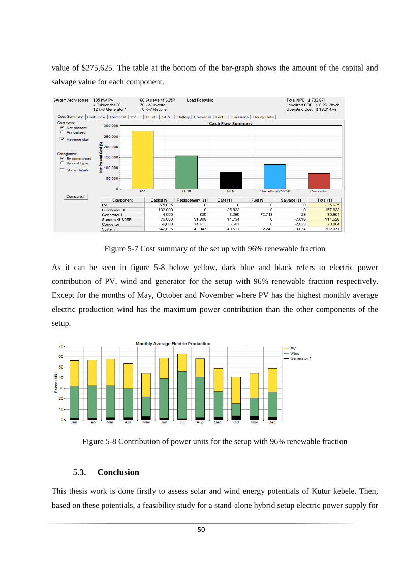
50
value of $275,625. The table at the bottom of the bar-graph shows the amount of the capital and
salvage value for each component.
Figure 5-7 Cost summary of the set up with 96% renewable fraction
As it can be seen in figure 5-8 below yellow, dark blue and black refers to electric power
contribution of PV, wind and generator for the setup with 96% renewable fraction respectively.
Except for the months of May, October and November where PV has the highest monthly average
electric production wind has the maximum power contribution than the other components of the
setup.
Figure 5-8 Contribution of power units for the setup with 96% renewable fraction
5.3. Conclusion
This thesis work is done firstly to assess solar and wind energy potentials of Kutur kebele. Then,
based on these potentials, a feasibility study for a stand-alone hybrid setup electric power supply for

51
the community is done. This is done first by considering the present number of households (i.e.
120), and then a simple load forecasting method is used to consider the change in the electric load of
the community with in the life span of the project which is 25 years. In addition to these, its cost is
compared against the cost required to electrify the area by extending MV distribution network from
the closest national grid.
The solar energy potential of the site is determined based on the data taken from NMSA. Since only
sunshine hour data are available, theoretically proved standard formulas are used to convert in to
solar radiation to determine the potential of the area. The result is also cross checked against the
satellite data obtained from NASA. However, the wind energy potential is taken from NASA since
there is no measured data for the selected site in NMSA. From the results, it can be observed that
the annual average wind speed of the selected site at ten meter height is 4.28m/s and its annual solar
radiation is 6.19kWh/m2/day. These results demonstrated the availability of extensive utilizable
solar and wind energy at the selected location.
The hybrid setup is then simulated using HOMER software in order to select the best optimized
result. For improving the viability of the supply the sources are integrated with other energy
conversion systems i.e. diesel generator and battery. The results of this study indicate that they can
be applicable to villages which have similar climatic conditions.
The feasibility study for the hybrid setup is based on the findings of the wind and solar energy
potentials at the particular site. With the potentials determined, two different approaches are
followed in the hybrid system design. In the first approach, the present load which is estimated
based on the current number of households of the area is used as input for the load profile. In the
second approach, the load attained at the end of the life span of the project which is obtained using a
simple load forecasting method is used as an input to simulate the hybrid setup.
The results obtained in the second approach have shown that the net present cost is more than three
folds of the first one. This has occurred due to the increase in the load of the community.
In the results, numerous alternative feasible hybrid setups, with different levels of contribution by
the renewable resources were obtained. Despite the numerous alternatives, the choice is restricted
by the varying net present cost, cost of energy and contribution of renewable energy resources of
each setup. The cost of energy of the hybrid setup is compared against the current global electricity
tariff and the tariff in the country, and it is found that the costs of the feasible setups obtained in the

52
study are higher than the current tariff in the country since the main source of energy is hydropower.
However, this will have a great role in alleviating deforestation, prevention of soil degradation and
improvement of the quality of life of the many people residing in the area by minimizing the health
problems caused by the smokes from fire-wood. Moreover, it will have a considerable effect in
minimizing the shortage of power within the country as well as in the reduction of pollutant
emissions in to the environment.
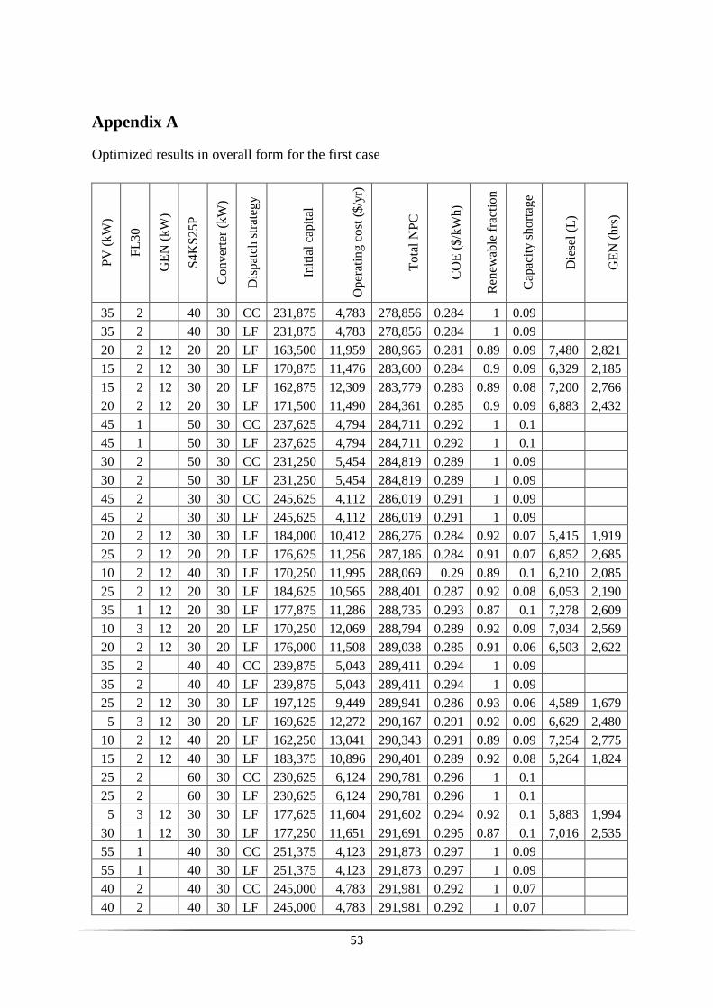
53
Appendix A
Optimized results in overall form for the first case
PV
(k
W)
FL
30
GE
N (
kW
)
S4
KS
25
P
Co
nv
erte
r (k
W)
Dis
pat
ch s
trat
egy
Init
ial
cap
ital
Op
erat
ing c
ost
($
/yr)
To
tal
NP
C
CO
E (
$/k
Wh
)
Ren
ewab
le f
ract
ion
Cap
acit
y s
ho
rtag
e
Die
sel
(L)
GE
N (
hrs
)
35 2 40 30 CC 231,875 4,783 278,856 0.284 1 0.09
35 2 40 30 LF 231,875 4,783 278,856 0.284 1 0.09
20 2 12 20 20 LF 163,500 11,959 280,965 0.281 0.89 0.09 7,480 2,821
15 2 12 30 30 LF 170,875 11,476 283,600 0.284 0.9 0.09 6,329 2,185
15 2 12 30 20 LF 162,875 12,309 283,779 0.283 0.89 0.08 7,200 2,766
20 2 12 20 30 LF 171,500 11,490 284,361 0.285 0.9 0.09 6,883 2,432
45 1 50 30 CC 237,625 4,794 284,711 0.292 1 0.1
45 1 50 30 LF 237,625 4,794 284,711 0.292 1 0.1
30 2 50 30 CC 231,250 5,454 284,819 0.289 1 0.09
30 2 50 30 LF 231,250 5,454 284,819 0.289 1 0.09
45 2 30 30 CC 245,625 4,112 286,019 0.291 1 0.09
45 2 30 30 LF 245,625 4,112 286,019 0.291 1 0.09
20 2 12 30 30 LF 184,000 10,412 286,276 0.284 0.92 0.07 5,415 1,919
25 2 12 20 20 LF 176,625 11,256 287,186 0.284 0.91 0.07 6,852 2,685
10 2 12 40 30 LF 170,250 11,995 288,069 0.29 0.89 0.1 6,210 2,085
25 2 12 20 30 LF 184,625 10,565 288,401 0.287 0.92 0.08 6,053 2,190
35 1 12 20 30 LF 177,875 11,286 288,735 0.293 0.87 0.1 7,278 2,609
10 3 12 20 20 LF 170,250 12,069 288,794 0.289 0.92 0.09 7,034 2,569
20 2 12 30 20 LF 176,000 11,508 289,038 0.285 0.91 0.06 6,503 2,622
35 2 40 40 CC 239,875 5,043 289,411 0.294 1 0.09
35 2 40 40 LF 239,875 5,043 289,411 0.294 1 0.09
25 2 12 30 30 LF 197,125 9,449 289,941 0.286 0.93 0.06 4,589 1,679
5 3 12 30 20 LF 169,625 12,272 290,167 0.291 0.92 0.09 6,629 2,480
10 2 12 40 20 LF 162,250 13,041 290,343 0.291 0.89 0.09 7,254 2,775
15 2 12 40 30 LF 183,375 10,896 290,401 0.289 0.92 0.08 5,264 1,824
25 2 60 30 CC 230,625 6,124 290,781 0.296 1 0.1
25 2 60 30 LF 230,625 6,124 290,781 0.296 1 0.1
5 3 12 30 30 LF 177,625 11,604 291,602 0.294 0.92 0.1 5,883 1,994
30 1 12 30 30 LF 177,250 11,651 291,691 0.295 0.87 0.1 7,016 2,535
55 1 40 30 CC 251,375 4,123 291,873 0.297 1 0.09
55 1 40 30 LF 251,375 4,123 291,873 0.297 1 0.09
40 2 40 30 CC 245,000 4,783 291,981 0.292 1 0.07
40 2 40 30 LF 245,000 4,783 291,981 0.292 1 0.07
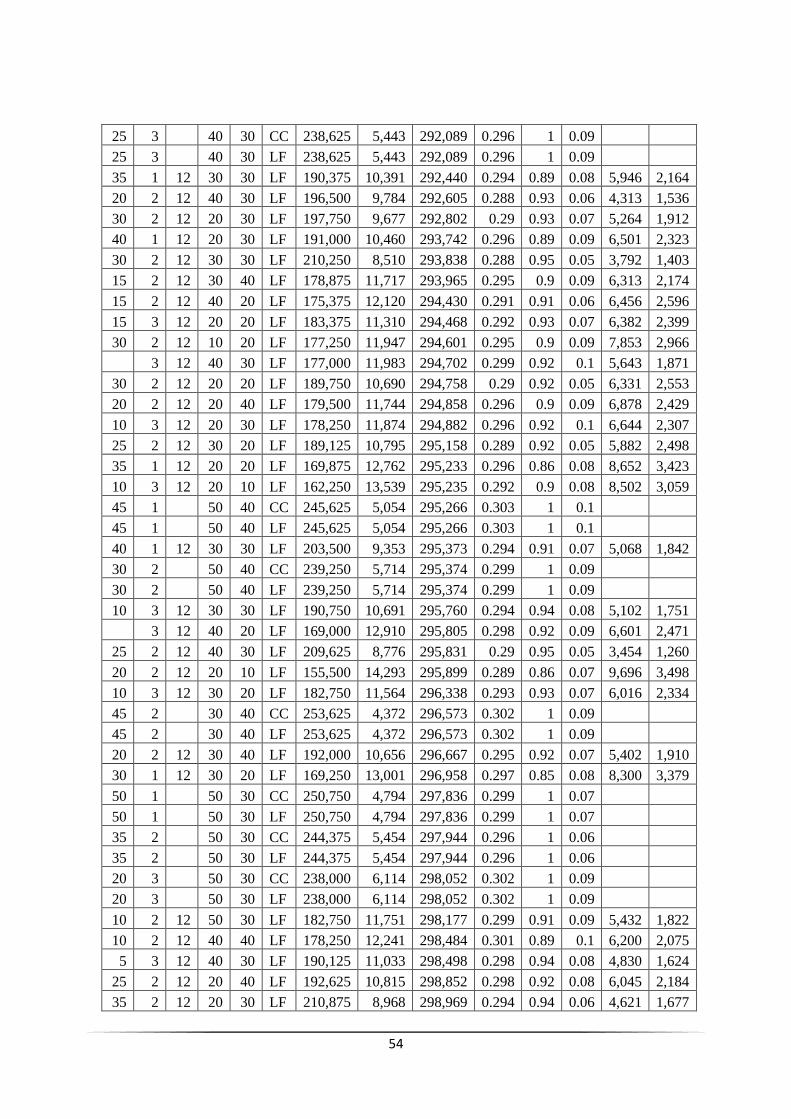
54
25 3 40 30 CC 238,625 5,443 292,089 0.296 1 0.09
25 3 40 30 LF 238,625 5,443 292,089 0.296 1 0.09
35 1 12 30 30 LF 190,375 10,391 292,440 0.294 0.89 0.08 5,946 2,164
20 2 12 40 30 LF 196,500 9,784 292,605 0.288 0.93 0.06 4,313 1,536
30 2 12 20 30 LF 197,750 9,677 292,802 0.29 0.93 0.07 5,264 1,912
40 1 12 20 30 LF 191,000 10,460 293,742 0.296 0.89 0.09 6,501 2,323
30 2 12 30 30 LF 210,250 8,510 293,838 0.288 0.95 0.05 3,792 1,403
15 2 12 30 40 LF 178,875 11,717 293,965 0.295 0.9 0.09 6,313 2,174
15 2 12 40 20 LF 175,375 12,120 294,430 0.291 0.91 0.06 6,456 2,596
15 3 12 20 20 LF 183,375 11,310 294,468 0.292 0.93 0.07 6,382 2,399
30 2 12 10 20 LF 177,250 11,947 294,601 0.295 0.9 0.09 7,853 2,966
3 12 40 30 LF 177,000 11,983 294,702 0.299 0.92 0.1 5,643 1,871
30 2 12 20 20 LF 189,750 10,690 294,758 0.29 0.92 0.05 6,331 2,553
20 2 12 20 40 LF 179,500 11,744 294,858 0.296 0.9 0.09 6,878 2,429
10 3 12 20 30 LF 178,250 11,874 294,882 0.296 0.92 0.1 6,644 2,307
25 2 12 30 20 LF 189,125 10,795 295,158 0.289 0.92 0.05 5,882 2,498
35 1 12 20 20 LF 169,875 12,762 295,233 0.296 0.86 0.08 8,652 3,423
10 3 12 20 10 LF 162,250 13,539 295,235 0.292 0.9 0.08 8,502 3,059
45 1 50 40 CC 245,625 5,054 295,266 0.303 1 0.1
45 1 50 40 LF 245,625 5,054 295,266 0.303 1 0.1
40 1 12 30 30 LF 203,500 9,353 295,373 0.294 0.91 0.07 5,068 1,842
30 2 50 40 CC 239,250 5,714 295,374 0.299 1 0.09
30 2 50 40 LF 239,250 5,714 295,374 0.299 1 0.09
10 3 12 30 30 LF 190,750 10,691 295,760 0.294 0.94 0.08 5,102 1,751
3 12 40 20 LF 169,000 12,910 295,805 0.298 0.92 0.09 6,601 2,471
25 2 12 40 30 LF 209,625 8,776 295,831 0.29 0.95 0.05 3,454 1,260
20 2 12 20 10 LF 155,500 14,293 295,899 0.289 0.86 0.07 9,696 3,498
10 3 12 30 20 LF 182,750 11,564 296,338 0.293 0.93 0.07 6,016 2,334
45 2 30 40 CC 253,625 4,372 296,573 0.302 1 0.09
45 2 30 40 LF 253,625 4,372 296,573 0.302 1 0.09
20 2 12 30 40 LF 192,000 10,656 296,667 0.295 0.92 0.07 5,402 1,910
30 1 12 30 20 LF 169,250 13,001 296,958 0.297 0.85 0.08 8,300 3,379
50 1 50 30 CC 250,750 4,794 297,836 0.299 1 0.07
50 1 50 30 LF 250,750 4,794 297,836 0.299 1 0.07
35 2 50 30 CC 244,375 5,454 297,944 0.296 1 0.06
35 2 50 30 LF 244,375 5,454 297,944 0.296 1 0.06
20 3 50 30 CC 238,000 6,114 298,052 0.302 1 0.09
20 3 50 30 LF 238,000 6,114 298,052 0.302 1 0.09
10 2 12 50 30 LF 182,750 11,751 298,177 0.299 0.91 0.09 5,432 1,822
10 2 12 40 40 LF 178,250 12,241 298,484 0.301 0.89 0.1 6,200 2,075
5 3 12 40 30 LF 190,125 11,033 298,498 0.298 0.94 0.08 4,830 1,624
25 2 12 20 40 LF 192,625 10,815 298,852 0.298 0.92 0.08 6,045 2,184
35 2 12 20 30 LF 210,875 8,968 298,969 0.294 0.94 0.06 4,621 1,677
55
15 3 12 20 30 LF 191,375 10,959 299,016 0.297 0.93 0.08 5,848 2,042
35 1 12 20 40 LF 185,875 11,520 299,034 0.304 0.87 0.1 7,257 2,594
50 2 30 30 CC 258,750 4,112 299,144 0.302 1 0.08
50 2 30 30 LF 258,750 4,112 299,144 0.302 1 0.08
35 1 12 40 30 LF 202,875 9,805 299,189 0.298 0.91 0.07 4,881 1,785
30 1 12 40 30 LF 189,750 11,143 299,204 0.3 0.88 0.08 6,017 2,181
35 3 30 30 CC 252,375 4,772 299,251 0.303 1 0.09
35 3 30 30 LF 252,375 4,772 299,251 0.303 1 0.09
35 2 12 30 30 LF 223,375 7,739 299,394 0.292 0.96 0.04 3,140 1,160
15 2 12 50 30 LF 195,875 10,562 299,619 0.296 0.93 0.07 4,413 1,523
30 2 12 10 30 LF 185,250 11,650 299,686 0.301 0.9 0.09 7,395 2,725
35 2 40 50 CC 247,875 5,303 299,966 0.305 1 0.09
35 2 40 50 LF 247,875 5,303 299,966 0.305 1 0.09
30 2 12 40 30 LF 222,750 7,866 300,012 0.292 0.96 0.04 2,673 985
20 2 12 40 20 LF 188,500 11,372 300,205 0.293 0.92 0.05 5,803 2,470
25 2 12 30 40 LF 205,125 9,691 300,311 0.296 0.93 0.06 4,574 1,668
15 3 12 30 30 LF 203,875 9,840 300,527 0.296 0.95 0.06 4,373 1,536
5 3 12 30 10 LF 161,625 14,146 300,575 0.297 0.9 0.08 8,451 3,029
45 1 12 30 30 LF 216,625 8,549 300,599 0.297 0.93 0.06 4,386 1,604
15 2 12 30 10 LF 154,875 14,841 300,654 0.294 0.86 0.07 9,594 3,453
15 2 12 40 40 LF 191,375 11,133 300,735 0.299 0.92 0.08 5,246 1,812
40 1 12 40 30 LF 216,000 8,663 301,093 0.297 0.93 0.05 3,915 1,434
25 2 60 40 CC 238,625 6,384 301,336 0.307 1 0.1
25 2 60 40 LF 238,625 6,384 301,336 0.307 1 0.1
5 3 12 40 20 LF 182,125 12,146 301,431 0.299 0.93 0.07 5,939 2,316
45 1 12 20 30 LF 204,125 9,916 301,528 0.301 0.9 0.08 5,956 2,117
20 2 12 50 30 LF 209,000 9,437 301,698 0.296 0.95 0.05 3,455 1,215
20 3 12 20 20 LF 196,500 10,726 301,854 0.296 0.94 0.06 5,872 2,291
5 3 12 30 40 LF 185,625 11,853 302,053 0.305 0.92 0.1 5,875 1,987
30 1 12 30 40 LF 185,250 11,893 302,074 0.306 0.87 0.1 7,002 2,524
20 3 12 10 20 LF 184,000 12,034 302,203 0.302 0.92 0.09 7,420 2,711
55 1 40 40 CC 259,375 4,383 302,428 0.307 1 0.08
55 1 40 40 LF 259,375 4,383 302,428 0.307 1 0.08
40 2 40 40 CC 253,000 5,043 302,536 0.302 1 0.07
40 2 40 40 LF 253,000 5,043 302,536 0.302 1 0.07
25 3 40 40 CC 246,625 5,703 302,644 0.307 1 0.09
25 3 40 40 LF 246,625 5,703 302,644 0.307 1 0.09
30 2 12 30 20 LF 202,250 10,221 302,647 0.294 0.94 0.03 5,385 2,383
35 1 12 30 40 LF 198,375 10,617 302,661 0.304 0.89 0.08 5,919 2,144
10 3 12 40 30 LF 203,250 10,131 302,765 0.299 0.95 0.06 4,059 1,387
15 3 12 30 20 LF 195,875 10,896 302,899 0.297 0.94 0.05 5,434 2,205
35 1 12 30 20 LF 182,375 12,271 302,912 0.3 0.87 0.06 7,665 3,241
20 2 12 40 40 LF 204,500 10,024 302,959 0.299 0.93 0.06 4,297 1,524
56
10 2 12 50 20 LF 174,750 13,055 302,985 0.301 0.9 0.07 6,688 2,635
30 2 12 20 40 LF 205,750 9,918 303,169 0.3 0.93 0.07 5,247 1,902
45 1 60 30 CC 250,125 5,464 303,799 0.305 1 0.07
45 1 60 30 LF 250,125 5,464 303,799 0.305 1 0.07
35 2 12 10 20 LF 190,375 11,556 303,881 0.303 0.91 0.08 7,502 2,863
30 2 60 30 CC 243,750 6,124 303,906 0.303 1 0.07
30 2 60 30 LF 243,750 6,124 303,906 0.303 1 0.07
40 1 12 20 40 LF 199,000 10,681 303,911 0.306 0.89 0.09 6,471 2,303
15 3 60 30 CC 237,375 6,784 304,014 0.31 1 0.1
15 3 60 30 LF 237,375 6,784 304,014 0.31 1 0.1
30 2 12 30 40 LF 218,250 8,743 304,125 0.298 0.95 0.05 3,770 1,387
15 3 12 20 10 LF 175,375 13,134 304,382 0.297 0.91 0.06 8,156 2,956
35 2 12 20 20 LF 202,875 10,337 304,409 0.297 0.93 0.04 5,979 2,464
20 3 12 20 30 LF 204,500 10,176 304,454 0.3 0.94 0.07 5,160 1,851
15 2 12 30 50 LF 186,875 11,977 304,520 0.305 0.9 0.09 6,313 2,174
3 12 50 30 LF 189,500 11,713 304,552 0.307 0.93 0.09 4,845 1,593
20 3 12 10 10 LF 176,000 13,107 304,741 0.302 0.91 0.08 8,604 3,077
60 1 40 30 CC 264,500 4,123 304,998 0.306 1 0.07
60 1 40 30 LF 264,500 4,123 304,998 0.306 1 0.07
3 12 40 40 LF 185,000 12,220 305,030 0.31 0.92 0.1 5,624 1,858
35 2 12 10 30 LF 198,375 10,859 305,042 0.305 0.92 0.08 6,714 2,459
45 2 40 30 CC 258,125 4,783 305,106 0.301 1 0.05
45 2 40 30 LF 258,125 4,783 305,106 0.301 1 0.05
30 3 40 30 CC 251,750 5,443 305,214 0.305 1 0.07
30 3 40 30 LF 251,750 5,443 305,214 0.305 1 0.07
20 2 12 20 50 LF 187,500 12,004 305,413 0.307 0.9 0.09 6,878 2,429
45 1 12 40 30 LF 229,125 7,768 305,426 0.299 0.95 0.04 3,156 1,164
10 3 12 20 40 LF 186,250 12,134 305,437 0.307 0.92 0.1 6,644 2,307
40 1 12 30 40 LF 211,500 9,568 305,478 0.304 0.91 0.07 5,032 1,816
25 2 12 50 30 LF 222,125 8,501 305,626 0.297 0.96 0.04 2,646 955
40 1 12 20 20 LF 183,000 12,487 305,658 0.304 0.87 0.07 8,299 3,352
45 1 50 50 CC 253,625 5,314 305,821 0.313 1 0.1
45 1 50 50 LF 253,625 5,314 305,821 0.313 1 0.1
30 2 50 50 CC 247,250 5,974 305,929 0.31 1 0.09
30 2 50 50 LF 247,250 5,974 305,929 0.31 1 0.09
25 2 12 40 40 LF 217,625 9,006 306,087 0.3 0.95 0.05 3,430 1,243
10 3 12 30 40 LF 198,750 10,932 306,132 0.304 0.94 0.08 5,087 1,741
20 3 12 30 30 LF 217,000 9,099 306,374 0.299 0.96 0.05 3,737 1,355
35 2 12 40 30 LF 235,875 7,197 306,571 0.297 0.97 0.03 2,098 780
40 2 12 30 30 LF 236,500 7,153 306,764 0.298 0.97 0.03 2,636 978
40 2 12 20 30 LF 224,000 8,435 306,854 0.3 0.95 0.05 4,140 1,488
45 2 30 50 CC 261,625 4,633 307,128 0.313 1 0.09
45 2 30 50 LF 261,625 4,633 307,128 0.313 1 0.09
57
20 2 12 30 50 LF 200,000 10,916 307,222 0.305 0.92 0.07 5,402 1,910
15 3 12 40 30 LF 216,375 9,252 307,250 0.3 0.96 0.05 3,305 1,159
25 2 12 20 10 LF 168,625 14,119 307,311 0.298 0.87 0.06 9,547 3,454
5 4 12 20 20 LF 190,125 11,931 307,320 0.308 0.94 0.09 6,364 2,308
25 2 12 40 20 LF 201,625 10,761 307,327 0.298 0.93 0.03 5,270 2,366
10 3 12 40 20 LF 195,250 11,445 307,673 0.302 0.94 0.05 5,330 2,173
35 3 40 20 CC 256,875 5,183 307,784 0.307 1 0.1
35 3 40 20 LF 256,875 5,183 307,784 0.307 1 0.1
10 2 12 40 10 LF 154,250 15,645 307,924 0.302 0.85 0.08 9,709 3,483
15 2 12 50 20 LF 187,875 12,228 307,990 0.302 0.91 0.05 5,968 2,490
30 1 12 40 20 LF 181,750 12,870 308,167 0.305 0.87 0.06 7,602 3,229
35 1 12 50 30 LF 215,375 9,468 308,371 0.304 0.92 0.06 4,029 1,469
50 1 50 40 CC 258,750 5,054 308,391 0.309 1 0.07
50 1 50 40 LF 258,750 5,054 308,391 0.309 1 0.07
35 2 50 40 CC 252,375 5,714 308,499 0.307 1 0.06
35 2 50 40 LF 252,375 5,714 308,499 0.307 1 0.06
10 2 12 50 40 LF 190,750 11,992 308,547 0.309 0.91 0.09 5,418 1,811
20 3 50 40 CC 246,000 6,374 308,607 0.313 1 0.09
20 3 50 40 LF 246,000 6,374 308,607 0.313 1 0.09
3 12 40 10 LF 161,000 15,031 308,640 0.307 0.89 0.09 8,635 3,075
5 3 12 50 30 LF 202,625 10,796 308,674 0.306 0.95 0.07 4,061 1,353
5 3 12 40 40 LF 198,125 11,271 308,838 0.309 0.94 0.08 4,813 1,611
4 12 30 20 LF 189,500 12,160 308,947 0.309 0.94 0.08 5,979 2,229
30 1 12 50 30 LF 202,250 10,871 309,034 0.308 0.9 0.07 5,217 1,897
10 2 12 40 50 LF 186,250 12,501 309,039 0.312 0.89 0.1 6,200 2,075
3 12 50 20 LF 181,500 12,987 309,065 0.309 0.92 0.08 6,088 2,346
50 1 12 30 30 LF 229,750 8,084 309,155 0.303 0.94 0.05 3,921 1,449
35 2 12 20 40 LF 218,875 9,198 309,219 0.304 0.94 0.06 4,596 1,660
25 3 12 10 20 LF 197,125 11,418 309,282 0.307 0.93 0.08 6,879 2,577
35 1 12 40 40 LF 210,875 10,020 309,296 0.308 0.91 0.07 4,844 1,760
25 2 12 20 50 LF 200,625 11,075 309,407 0.308 0.92 0.08 6,045 2,184
15 3 12 20 40 LF 199,375 11,212 309,510 0.308 0.93 0.08 5,843 2,039
30 1 12 40 40 LF 197,750 11,378 309,513 0.311 0.88 0.08 5,997 2,167
25 3 12 20 20 LF 209,625 10,171 309,531 0.302 0.95 0.05 5,390 2,180
35 1 12 20 50 LF 193,875 11,780 309,589 0.314 0.87 0.1 7,257 2,594
35 2 12 30 40 LF 231,375 7,964 309,603 0.302 0.96 0.04 3,111 1,141
10 2 12 60 30 LF 195,250 11,642 309,608 0.308 0.92 0.08 4,772 1,589
50 2 30 40 CC 266,750 4,372 309,698 0.312 1 0.08
58
Appendix B
Optimized result in overall form for efficient lamps
PV
(k
W)
FL
30
GE
N (
kW
)
S4
KS
25
P
Co
nv
erte
r (k
W)
Dis
pat
ch s
trat
egy
Init
ial
cap
ital
Op
erat
ing c
ost
($
/yr)
To
tal
NP
C
CO
E (
$/k
Wh
)
Ren
ewab
le f
ract
ion
Cap
acit
y s
ho
rtag
e
Die
sel
(L)
GE
N (
hrs
)
5 2 12 10 10 LF $103,625 13,175 $194,174 0.345 0.85 0.1 9,005 3,395
15 1 12 10 10 LF $96,875 14,782 $198,470 0.346 0.77 0.08 10,818 4,151
10 1 12 20 10 LF $96,250 15,085 $199,926 0.352 0.75 0.09 10,591 4,020
5 2 12 20 10 LF $116,125 12,209 $200,037 0.35 0.87 0.07 7,736 2,962
5 2 12 10 20 LF $111,625 12,882 $200,162 0.357 0.86 0.1 8,588 3,180
10 2 12 10 10 LF $116,750 12,298 $201,271 0.35 0.87 0.07 8,283 3,195
5 2 12 20 20 LF $124,125 11,281 $201,657 0.355 0.88 0.07 6,823 2,546
15 1 12 20 10 LF $109,375 13,669 $203,322 0.352 0.79 0.07 9,437 3,658
20 1 12 10 10 LF $110,000 13,613 $203,559 0.353 0.8 0.07 9,863 3,864
2 12 30 10 LF $115,500 12,889 $204,087 0.361 0.86 0.08 7,810 2,956
40 1 20 30 CC $187,000 2,509 $204,243 0.368 1 0.1
40 1 20 30 LF $187,000 2,509 $204,243 0.368 1 0.1
2 12 30 20 LF $123,500 11,768 $204,380 0.365 0.88 0.08 6,739 2,499
10 1 12 20 20 LF $104,250 14,577 $204,436 0.361 0.76 0.09 10,017 3,745
15 1 12 10 20 LF $104,875 14,660 $205,631 0.358 0.77 0.08 10,547 4,030
15 1 12 20 20 LF $117,375 13,025 $206,894 0.358 0.8 0.06 8,746 3,367
10 2 12 10 20 LF $124,750 11,973 $207,040 0.361 0.88 0.07 7,826 2,970
10 2 12 20 10 LF $129,250 11,350 $207,257 0.358 0.89 0.05 7,032 2,755
10 2 12 20 20 LF $137,250 10,226 $207,533 0.358 0.9 0.05 5,955 2,307
35 1 30 30 CC $186,375 3,105 $207,712 0.371 1 0.09
35 1 30 30 LF $186,375 3,105 $207,712 0.371 1 0.09
3 12 10 10 LF $123,500 12,277 $207,877 0.372 0.9 0.1 7,743 2,894
15 2 12 10 10 LF $129,875 11,376 $208,064 0.358 0.89 0.05 7,529 2,969
20 1 12 20 10 LF $122,500 12,565 $208,859 0.361 0.82 0.06 8,536 3,374
5 2 12 30 20 LF $136,625 10,567 $209,250 0.365 0.9 0.06 5,753 2,200
20 1 12 10 20 LF $118,000 13,282 $209,288 0.359 0.81 0.05 9,411 3,739
20 1 12 20 20 LF $130,500 11,514 $209,633 0.358 0.84 0.04 7,501 3,030
5 2 12 10 30 LF $119,625 13,098 $209,650 0.374 0.86 0.1 8,586 3,179
5 2 12 20 30 LF $132,125 11,293 $209,739 0.37 0.88 0.08 6,665 2,438
10 1 12 30 10 LF $108,750 14,762 $210,205 0.368 0.76 0.08 9,847 3,759
5 2 12 30 10 LF $128,625 12,005 $211,136 0.367 0.88 0.06 7,085 2,749
30 1 40 30 CC $185,750 3,700 $211,181 0.38 1 0.1
30 1 40 30 LF $185,750 3,700 $211,181 0.38 1 0.1
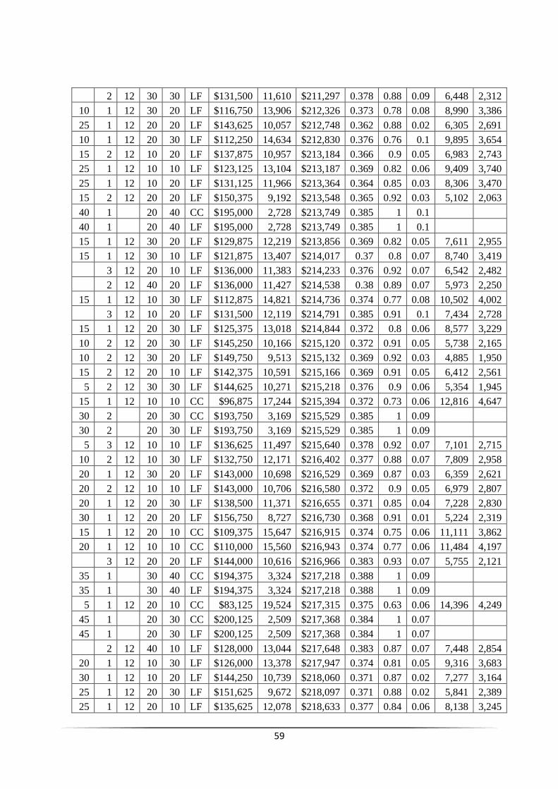
59
2 12 30 30 LF $131,500 11,610 $211,297 0.378 0.88 0.09 6,448 2,312
10 1 12 30 20 LF $116,750 13,906 $212,326 0.373 0.78 0.08 8,990 3,386
25 1 12 20 20 LF $143,625 10,057 $212,748 0.362 0.88 0.02 6,305 2,691
10 1 12 20 30 LF $112,250 14,634 $212,830 0.376 0.76 0.1 9,895 3,654
15 2 12 10 20 LF $137,875 10,957 $213,184 0.366 0.9 0.05 6,983 2,743
25 1 12 10 10 LF $123,125 13,104 $213,187 0.369 0.82 0.06 9,409 3,740
25 1 12 10 20 LF $131,125 11,966 $213,364 0.364 0.85 0.03 8,306 3,470
15 2 12 20 20 LF $150,375 9,192 $213,548 0.365 0.92 0.03 5,102 2,063
40 1 20 40 CC $195,000 2,728 $213,749 0.385 1 0.1
40 1 20 40 LF $195,000 2,728 $213,749 0.385 1 0.1
15 1 12 30 20 LF $129,875 12,219 $213,856 0.369 0.82 0.05 7,611 2,955
15 1 12 30 10 LF $121,875 13,407 $214,017 0.37 0.8 0.07 8,740 3,419
3 12 20 10 LF $136,000 11,383 $214,233 0.376 0.92 0.07 6,542 2,482
2 12 40 20 LF $136,000 11,427 $214,538 0.38 0.89 0.07 5,973 2,250
15 1 12 10 30 LF $112,875 14,821 $214,736 0.374 0.77 0.08 10,502 4,002
3 12 10 20 LF $131,500 12,119 $214,791 0.385 0.91 0.1 7,434 2,728
15 1 12 20 30 LF $125,375 13,018 $214,844 0.372 0.8 0.06 8,577 3,229
10 2 12 20 30 LF $145,250 10,166 $215,120 0.372 0.91 0.05 5,738 2,165
10 2 12 30 20 LF $149,750 9,513 $215,132 0.369 0.92 0.03 4,885 1,950
15 2 12 20 10 LF $142,375 10,591 $215,166 0.369 0.91 0.05 6,412 2,561
5 2 12 30 30 LF $144,625 10,271 $215,218 0.376 0.9 0.06 5,354 1,945
15 1 12 10 10 CC $96,875 17,244 $215,394 0.372 0.73 0.06 12,816 4,647
30 2 20 30 CC $193,750 3,169 $215,529 0.385 1 0.09
30 2 20 30 LF $193,750 3,169 $215,529 0.385 1 0.09
5 3 12 10 10 LF $136,625 11,497 $215,640 0.378 0.92 0.07 7,101 2,715
10 2 12 10 30 LF $132,750 12,171 $216,402 0.377 0.88 0.07 7,809 2,958
20 1 12 30 20 LF $143,000 10,698 $216,529 0.369 0.87 0.03 6,359 2,621
20 2 12 10 10 LF $143,000 10,706 $216,580 0.372 0.9 0.05 6,979 2,807
20 1 12 20 30 LF $138,500 11,371 $216,655 0.371 0.85 0.04 7,228 2,830
30 1 12 20 20 LF $156,750 8,727 $216,730 0.368 0.91 0.01 5,224 2,319
15 1 12 20 10 CC $109,375 15,647 $216,915 0.374 0.75 0.06 11,111 3,862
20 1 12 10 10 CC $110,000 15,560 $216,943 0.374 0.77 0.06 11,484 4,197
3 12 20 20 LF $144,000 10,616 $216,966 0.383 0.93 0.07 5,755 2,121
35 1 30 40 CC $194,375 3,324 $217,218 0.388 1 0.09
35 1 30 40 LF $194,375 3,324 $217,218 0.388 1 0.09
5 1 12 20 10 CC $83,125 19,524 $217,315 0.375 0.63 0.06 14,396 4,249
45 1 20 30 CC $200,125 2,509 $217,368 0.384 1 0.07
45 1 20 30 LF $200,125 2,509 $217,368 0.384 1 0.07
2 12 40 10 LF $128,000 13,044 $217,648 0.383 0.87 0.07 7,448 2,854
20 1 12 10 30 LF $126,000 13,378 $217,947 0.374 0.81 0.05 9,316 3,683
30 1 12 10 20 LF $144,250 10,739 $218,060 0.371 0.87 0.02 7,277 3,164
25 1 12 20 30 LF $151,625 9,672 $218,097 0.371 0.88 0.02 5,841 2,389
25 1 12 20 10 LF $135,625 12,078 $218,633 0.377 0.84 0.06 8,138 3,245
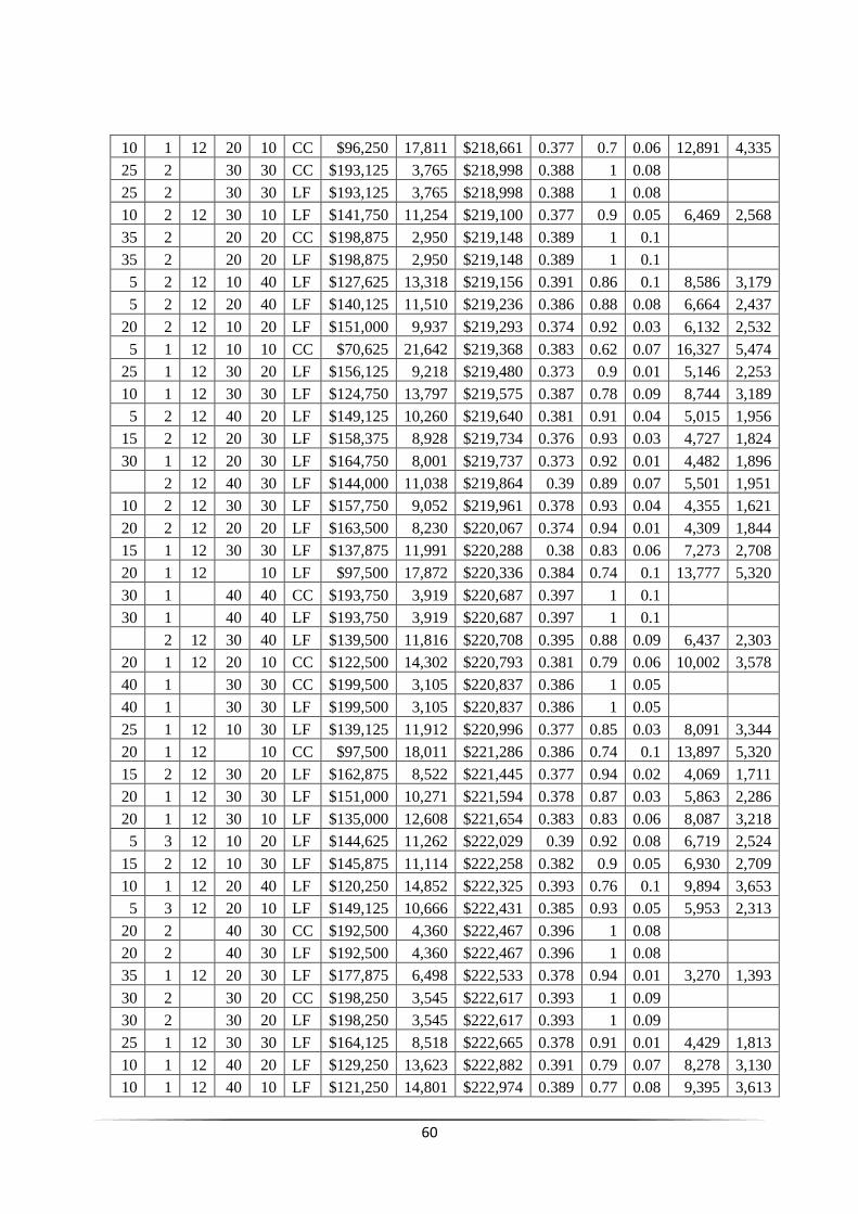
60
10 1 12 20 10 CC $96,250 17,811 $218,661 0.377 0.7 0.06 12,891 4,335
25 2 30 30 CC $193,125 3,765 $218,998 0.388 1 0.08
25 2 30 30 LF $193,125 3,765 $218,998 0.388 1 0.08
10 2 12 30 10 LF $141,750 11,254 $219,100 0.377 0.9 0.05 6,469 2,568
35 2 20 20 CC $198,875 2,950 $219,148 0.389 1 0.1
35 2 20 20 LF $198,875 2,950 $219,148 0.389 1 0.1
5 2 12 10 40 LF $127,625 13,318 $219,156 0.391 0.86 0.1 8,586 3,179
5 2 12 20 40 LF $140,125 11,510 $219,236 0.386 0.88 0.08 6,664 2,437
20 2 12 10 20 LF $151,000 9,937 $219,293 0.374 0.92 0.03 6,132 2,532
5 1 12 10 10 CC $70,625 21,642 $219,368 0.383 0.62 0.07 16,327 5,474
25 1 12 30 20 LF $156,125 9,218 $219,480 0.373 0.9 0.01 5,146 2,253
10 1 12 30 30 LF $124,750 13,797 $219,575 0.387 0.78 0.09 8,744 3,189
5 2 12 40 20 LF $149,125 10,260 $219,640 0.381 0.91 0.04 5,015 1,956
15 2 12 20 30 LF $158,375 8,928 $219,734 0.376 0.93 0.03 4,727 1,824
30 1 12 20 30 LF $164,750 8,001 $219,737 0.373 0.92 0.01 4,482 1,896
2 12 40 30 LF $144,000 11,038 $219,864 0.39 0.89 0.07 5,501 1,951
10 2 12 30 30 LF $157,750 9,052 $219,961 0.378 0.93 0.04 4,355 1,621
20 2 12 20 20 LF $163,500 8,230 $220,067 0.374 0.94 0.01 4,309 1,844
15 1 12 30 30 LF $137,875 11,991 $220,288 0.38 0.83 0.06 7,273 2,708
20 1 12 10 LF $97,500 17,872 $220,336 0.384 0.74 0.1 13,777 5,320
30 1 40 40 CC $193,750 3,919 $220,687 0.397 1 0.1
30 1 40 40 LF $193,750 3,919 $220,687 0.397 1 0.1
2 12 30 40 LF $139,500 11,816 $220,708 0.395 0.88 0.09 6,437 2,303
20 1 12 20 10 CC $122,500 14,302 $220,793 0.381 0.79 0.06 10,002 3,578
40 1 30 30 CC $199,500 3,105 $220,837 0.386 1 0.05
40 1 30 30 LF $199,500 3,105 $220,837 0.386 1 0.05
25 1 12 10 30 LF $139,125 11,912 $220,996 0.377 0.85 0.03 8,091 3,344
20 1 12 10 CC $97,500 18,011 $221,286 0.386 0.74 0.1 13,897 5,320
15 2 12 30 20 LF $162,875 8,522 $221,445 0.377 0.94 0.02 4,069 1,711
20 1 12 30 30 LF $151,000 10,271 $221,594 0.378 0.87 0.03 5,863 2,286
20 1 12 30 10 LF $135,000 12,608 $221,654 0.383 0.83 0.06 8,087 3,218
5 3 12 10 20 LF $144,625 11,262 $222,029 0.39 0.92 0.08 6,719 2,524
15 2 12 10 30 LF $145,875 11,114 $222,258 0.382 0.9 0.05 6,930 2,709
10 1 12 20 40 LF $120,250 14,852 $222,325 0.393 0.76 0.1 9,894 3,653
5 3 12 20 10 LF $149,125 10,666 $222,431 0.385 0.93 0.05 5,953 2,313
20 2 40 30 CC $192,500 4,360 $222,467 0.396 1 0.08
20 2 40 30 LF $192,500 4,360 $222,467 0.396 1 0.08
35 1 12 20 30 LF $177,875 6,498 $222,533 0.378 0.94 0.01 3,270 1,393
30 2 30 20 CC $198,250 3,545 $222,617 0.393 1 0.09
30 2 30 20 LF $198,250 3,545 $222,617 0.393 1 0.09
25 1 12 30 30 LF $164,125 8,518 $222,665 0.378 0.91 0.01 4,429 1,813
10 1 12 40 20 LF $129,250 13,623 $222,882 0.391 0.79 0.07 8,278 3,130
10 1 12 40 10 LF $121,250 14,801 $222,974 0.389 0.77 0.08 9,395 3,613
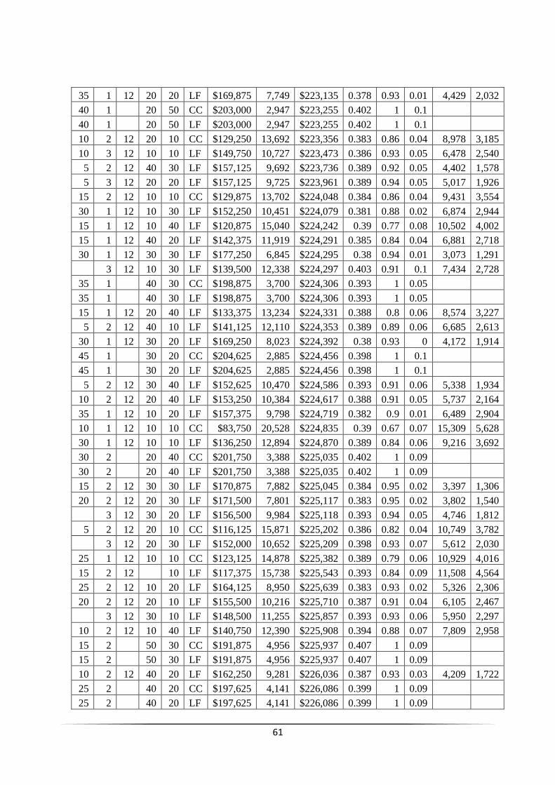
61
35 1 12 20 20 LF $169,875 7,749 $223,135 0.378 0.93 0.01 4,429 2,032
40 1 20 50 CC $203,000 2,947 $223,255 0.402 1 0.1
40 1 20 50 LF $203,000 2,947 $223,255 0.402 1 0.1
10 2 12 20 10 CC $129,250 13,692 $223,356 0.383 0.86 0.04 8,978 3,185
10 3 12 10 10 LF $149,750 10,727 $223,473 0.386 0.93 0.05 6,478 2,540
5 2 12 40 30 LF $157,125 9,692 $223,736 0.389 0.92 0.05 4,402 1,578
5 3 12 20 20 LF $157,125 9,725 $223,961 0.389 0.94 0.05 5,017 1,926
15 2 12 10 10 CC $129,875 13,702 $224,048 0.384 0.86 0.04 9,431 3,554
30 1 12 10 30 LF $152,250 10,451 $224,079 0.381 0.88 0.02 6,874 2,944
15 1 12 10 40 LF $120,875 15,040 $224,242 0.39 0.77 0.08 10,502 4,002
15 1 12 40 20 LF $142,375 11,919 $224,291 0.385 0.84 0.04 6,881 2,718
30 1 12 30 30 LF $177,250 6,845 $224,295 0.38 0.94 0.01 3,073 1,291
3 12 10 30 LF $139,500 12,338 $224,297 0.403 0.91 0.1 7,434 2,728
35 1 40 30 CC $198,875 3,700 $224,306 0.393 1 0.05
35 1 40 30 LF $198,875 3,700 $224,306 0.393 1 0.05
15 1 12 20 40 LF $133,375 13,234 $224,331 0.388 0.8 0.06 8,574 3,227
5 2 12 40 10 LF $141,125 12,110 $224,353 0.389 0.89 0.06 6,685 2,613
30 1 12 30 20 LF $169,250 8,023 $224,392 0.38 0.93 0 4,172 1,914
45 1 30 20 CC $204,625 2,885 $224,456 0.398 1 0.1
45 1 30 20 LF $204,625 2,885 $224,456 0.398 1 0.1
5 2 12 30 40 LF $152,625 10,470 $224,586 0.393 0.91 0.06 5,338 1,934
10 2 12 20 40 LF $153,250 10,384 $224,617 0.388 0.91 0.05 5,737 2,164
35 1 12 10 20 LF $157,375 9,798 $224,719 0.382 0.9 0.01 6,489 2,904
10 1 12 10 10 CC $83,750 20,528 $224,835 0.39 0.67 0.07 15,309 5,628
30 1 12 10 10 LF $136,250 12,894 $224,870 0.389 0.84 0.06 9,216 3,692
30 2 20 40 CC $201,750 3,388 $225,035 0.402 1 0.09
30 2 20 40 LF $201,750 3,388 $225,035 0.402 1 0.09
15 2 12 30 30 LF $170,875 7,882 $225,045 0.384 0.95 0.02 3,397 1,306
20 2 12 20 30 LF $171,500 7,801 $225,117 0.383 0.95 0.02 3,802 1,540
3 12 30 20 LF $156,500 9,984 $225,118 0.393 0.94 0.05 4,746 1,812
5 2 12 20 10 CC $116,125 15,871 $225,202 0.386 0.82 0.04 10,749 3,782
3 12 20 30 LF $152,000 10,652 $225,209 0.398 0.93 0.07 5,612 2,030
25 1 12 10 10 CC $123,125 14,878 $225,382 0.389 0.79 0.06 10,929 4,016
15 2 12 10 LF $117,375 15,738 $225,543 0.393 0.84 0.09 11,508 4,564
25 2 12 10 20 LF $164,125 8,950 $225,639 0.383 0.93 0.02 5,326 2,306
20 2 12 20 10 LF $155,500 10,216 $225,710 0.387 0.91 0.04 6,105 2,467
3 12 30 10 LF $148,500 11,255 $225,857 0.393 0.93 0.06 5,950 2,297
10 2 12 10 40 LF $140,750 12,390 $225,908 0.394 0.88 0.07 7,809 2,958
15 2 50 30 CC $191,875 4,956 $225,937 0.407 1 0.09
15 2 50 30 LF $191,875 4,956 $225,937 0.407 1 0.09
10 2 12 40 20 LF $162,250 9,281 $226,036 0.387 0.93 0.03 4,209 1,722
25 2 40 20 CC $197,625 4,141 $226,086 0.399 1 0.09
25 2 40 20 LF $197,625 4,141 $226,086 0.399 1 0.09
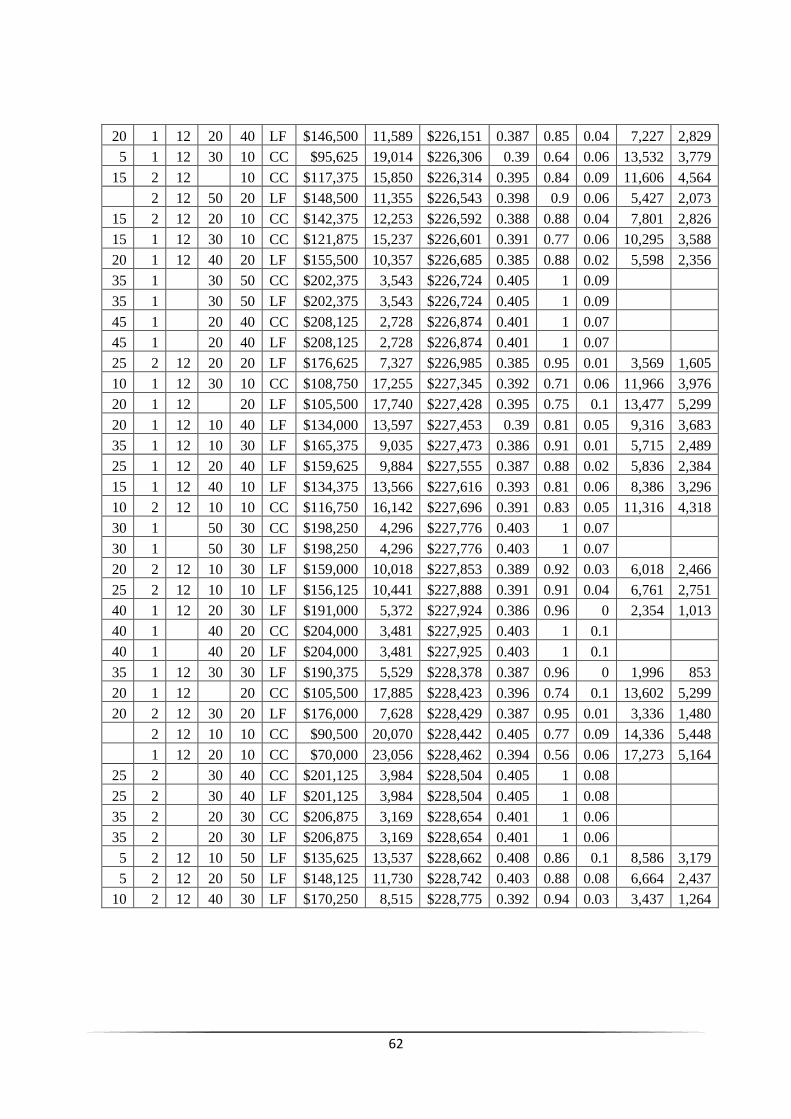
62
20 1 12 20 40 LF $146,500 11,589 $226,151 0.387 0.85 0.04 7,227 2,829
5 1 12 30 10 CC $95,625 19,014 $226,306 0.39 0.64 0.06 13,532 3,779
15 2 12 10 CC $117,375 15,850 $226,314 0.395 0.84 0.09 11,606 4,564
2 12 50 20 LF $148,500 11,355 $226,543 0.398 0.9 0.06 5,427 2,073
15 2 12 20 10 CC $142,375 12,253 $226,592 0.388 0.88 0.04 7,801 2,826
15 1 12 30 10 CC $121,875 15,237 $226,601 0.391 0.77 0.06 10,295 3,588
20 1 12 40 20 LF $155,500 10,357 $226,685 0.385 0.88 0.02 5,598 2,356
35 1 30 50 CC $202,375 3,543 $226,724 0.405 1 0.09
35 1 30 50 LF $202,375 3,543 $226,724 0.405 1 0.09
45 1 20 40 CC $208,125 2,728 $226,874 0.401 1 0.07
45 1 20 40 LF $208,125 2,728 $226,874 0.401 1 0.07
25 2 12 20 20 LF $176,625 7,327 $226,985 0.385 0.95 0.01 3,569 1,605
10 1 12 30 10 CC $108,750 17,255 $227,345 0.392 0.71 0.06 11,966 3,976
20 1 12 20 LF $105,500 17,740 $227,428 0.395 0.75 0.1 13,477 5,299
20 1 12 10 40 LF $134,000 13,597 $227,453 0.39 0.81 0.05 9,316 3,683
35 1 12 10 30 LF $165,375 9,035 $227,473 0.386 0.91 0.01 5,715 2,489
25 1 12 20 40 LF $159,625 9,884 $227,555 0.387 0.88 0.02 5,836 2,384
15 1 12 40 10 LF $134,375 13,566 $227,616 0.393 0.81 0.06 8,386 3,296
10 2 12 10 10 CC $116,750 16,142 $227,696 0.391 0.83 0.05 11,316 4,318
30 1 50 30 CC $198,250 4,296 $227,776 0.403 1 0.07
30 1 50 30 LF $198,250 4,296 $227,776 0.403 1 0.07
20 2 12 10 30 LF $159,000 10,018 $227,853 0.389 0.92 0.03 6,018 2,466
25 2 12 10 10 LF $156,125 10,441 $227,888 0.391 0.91 0.04 6,761 2,751
40 1 12 20 30 LF $191,000 5,372 $227,924 0.386 0.96 0 2,354 1,013
40 1 40 20 CC $204,000 3,481 $227,925 0.403 1 0.1
40 1 40 20 LF $204,000 3,481 $227,925 0.403 1 0.1
35 1 12 30 30 LF $190,375 5,529 $228,378 0.387 0.96 0 1,996 853
20 1 12 20 CC $105,500 17,885 $228,423 0.396 0.74 0.1 13,602 5,299
20 2 12 30 20 LF $176,000 7,628 $228,429 0.387 0.95 0.01 3,336 1,480
2 12 10 10 CC $90,500 20,070 $228,442 0.405 0.77 0.09 14,336 5,448
1 12 20 10 CC $70,000 23,056 $228,462 0.394 0.56 0.06 17,273 5,164
25 2 30 40 CC $201,125 3,984 $228,504 0.405 1 0.08
25 2 30 40 LF $201,125 3,984 $228,504 0.405 1 0.08
35 2 20 30 CC $206,875 3,169 $228,654 0.401 1 0.06
35 2 20 30 LF $206,875 3,169 $228,654 0.401 1 0.06
5 2 12 10 50 LF $135,625 13,537 $228,662 0.408 0.86 0.1 8,586 3,179
5 2 12 20 50 LF $148,125 11,730 $228,742 0.403 0.88 0.08 6,664 2,437
10 2 12 40 30 LF $170,250 8,515 $228,775 0.392 0.94 0.03 3,437 1,264
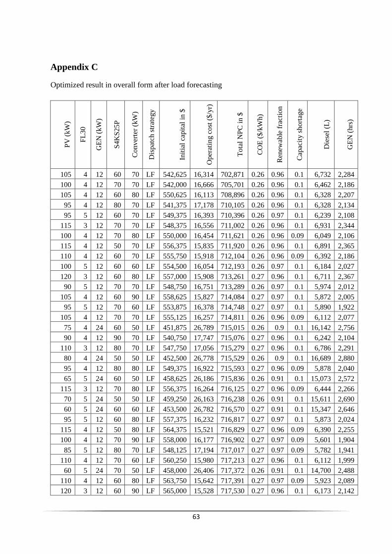
63
Appendix C
Optimized result in overall form after load forecasting
PV
(k
W)
FL
30
GE
N (
kW
)
S4
KS
25
P
Co
nv
erte
r (k
W)
Dis
pat
ch s
trat
egy
Init
ial
cap
ital
in
$
Op
erat
ing c
ost
($
/yr)
To
tal
NP
C i
n $
CO
E (
$/k
Wh
)
Ren
ewab
le f
ract
ion
Cap
acit
y s
ho
rtag
e
Die
sel
(L)
GE
N (
hrs
)
105 4 12 60 70 LF 542,625 16,314 702,871 0.26 0.96 0.1 6,732 2,284
100 4 12 70 70 LF 542,000 16,666 705,701 0.26 0.96 0.1 6,462 2,186
105 4 12 60 80 LF 550,625 16,113 708,896 0.26 0.96 0.1 6,328 2,207
95 4 12 80 70 LF 541,375 17,178 710,105 0.26 0.96 0.1 6,328 2,134
95 5 12 60 70 LF 549,375 16,393 710,396 0.26 0.97 0.1 6,239 2,108
115 3 12 70 70 LF 548,375 16,556 711,002 0.26 0.96 0.1 6,931 2,344
100 4 12 70 80 LF 550,000 16,454 711,621 0.26 0.96 0.09 6,049 2,106
115 4 12 50 70 LF 556,375 15,835 711,920 0.26 0.96 0.1 6,891 2,365
110 4 12 60 70 LF 555,750 15,918 712,104 0.26 0.96 0.09 6,392 2,186
100 5 12 60 60 LF 554,500 16,054 712,193 0.26 0.97 0.1 6,184 2,027
120 3 12 60 80 LF 557,000 15,908 713,261 0.27 0.96 0.1 6,711 2,367
90 5 12 70 70 LF 548,750 16,751 713,289 0.26 0.97 0.1 5,974 2,012
105 4 12 60 90 LF 558,625 15,827 714,084 0.27 0.97 0.1 5,872 2,005
95 5 12 70 60 LF 553,875 16,378 714,748 0.27 0.97 0.1 5,890 1,922
105 4 12 70 70 LF 555,125 16,257 714,811 0.26 0.96 0.09 6,112 2,077
75 4 24 60 50 LF 451,875 26,789 715,015 0.26 0.9 0.1 16,142 2,756
90 4 12 90 70 LF 540,750 17,747 715,076 0.27 0.96 0.1 6,242 2,104
110 3 12 80 70 LF 547,750 17,056 715,279 0.27 0.96 0.1 6,786 2,291
80 4 24 50 50 LF 452,500 26,778 715,529 0.26 0.9 0.1 16,689 2,880
95 4 12 80 80 LF 549,375 16,922 715,593 0.27 0.96 0.09 5,878 2,040
65 5 24 60 50 LF 458,625 26,186 715,836 0.26 0.91 0.1 15,073 2,572
115 3 12 70 80 LF 556,375 16,264 716,125 0.27 0.96 0.09 6,444 2,266
70 5 24 50 50 LF 459,250 26,163 716,238 0.26 0.91 0.1 15,611 2,690
60 5 24 60 60 LF 453,500 26,782 716,570 0.27 0.91 0.1 15,347 2,646
95 5 12 60 80 LF 557,375 16,232 716,817 0.27 0.97 0.1 5,873 2,024
115 4 12 50 80 LF 564,375 15,521 716,829 0.27 0.96 0.09 6,390 2,255
100 4 12 70 90 LF 558,000 16,177 716,902 0.27 0.97 0.09 5,601 1,904
85 5 12 80 70 LF 548,125 17,194 717,017 0.27 0.97 0.09 5,782 1,941
110 4 12 70 60 LF 560,250 15,980 717,213 0.27 0.96 0.1 6,112 1,999
60 5 24 70 50 LF 458,000 26,406 717,372 0.26 0.91 0.1 14,700 2,488
110 4 12 60 80 LF 563,750 15,642 717,391 0.27 0.97 0.09 5,923 2,089
120 3 12 60 90 LF 565,000 15,528 717,530 0.27 0.96 0.1 6,173 2,142
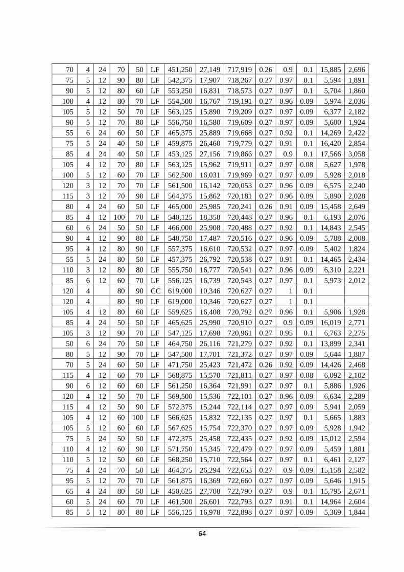
64
70 4 24 70 50 LF 451,250 27,149 717,919 0.26 0.9 0.1 15,885 2,696
75 5 12 90 80 LF 542,375 17,907 718,267 0.27 0.97 0.1 5,594 1,891
90 5 12 80 60 LF 553,250 16,831 718,573 0.27 0.97 0.1 5,704 1,860
100 4 12 80 70 LF 554,500 16,767 719,191 0.27 0.96 0.09 5,974 2,036
105 5 12 50 70 LF 563,125 15,890 719,209 0.27 0.97 0.09 6,377 2,182
90 5 12 70 80 LF 556,750 16,580 719,609 0.27 0.97 0.09 5,600 1,924
55 6 24 60 50 LF 465,375 25,889 719,668 0.27 0.92 0.1 14,269 2,422
75 5 24 40 50 LF 459,875 26,460 719,779 0.27 0.91 0.1 16,420 2,854
85 4 24 40 50 LF 453,125 27,156 719,866 0.27 0.9 0.1 17,566 3,058
105 4 12 70 80 LF 563,125 15,962 719,911 0.27 0.97 0.08 5,627 1,978
100 5 12 60 70 LF 562,500 16,031 719,969 0.27 0.97 0.09 5,928 2,018
120 3 12 70 70 LF 561,500 16,142 720,053 0.27 0.96 0.09 6,575 2,240
115 3 12 70 90 LF 564,375 15,862 720,181 0.27 0.96 0.09 5,890 2,028
80 4 24 60 50 LF 465,000 25,985 720,241 0.26 0.91 0.09 15,458 2,649
85 4 12 100 70 LF 540,125 18,358 720,448 0.27 0.96 0.1 6,193 2,076
60 6 24 50 50 LF 466,000 25,908 720,488 0.27 0.92 0.1 14,843 2,545
90 4 12 90 80 LF 548,750 17,487 720,516 0.27 0.96 0.09 5,788 2,008
95 4 12 80 90 LF 557,375 16,610 720,532 0.27 0.97 0.09 5,402 1,824
55 5 24 80 50 LF 457,375 26,792 720,538 0.27 0.91 0.1 14,465 2,434
110 3 12 80 80 LF 555,750 16,777 720,541 0.27 0.96 0.09 6,310 2,221
85 6 12 60 70 LF 556,125 16,739 720,543 0.27 0.97 0.1 5,973 2,012
120 4 80 90 CC 619,000 10,346 720,627 0.27 1 0.1
120 4 80 90 LF 619,000 10,346 720,627 0.27 1 0.1
105 4 12 80 60 LF 559,625 16,408 720,792 0.27 0.96 0.1 5,906 1,928
85 4 24 50 50 LF 465,625 25,990 720,910 0.27 0.9 0.09 16,019 2,771
105 3 12 90 70 LF 547,125 17,698 720,961 0.27 0.95 0.1 6,763 2,275
50 6 24 70 50 LF 464,750 26,116 721,279 0.27 0.92 0.1 13,899 2,341
80 5 12 90 70 LF 547,500 17,701 721,372 0.27 0.97 0.09 5,644 1,887
70 5 24 60 50 LF 471,750 25,423 721,472 0.26 0.92 0.09 14,426 2,468
115 4 12 60 70 LF 568,875 15,570 721,811 0.27 0.97 0.08 6,092 2,102
90 6 12 60 60 LF 561,250 16,364 721,991 0.27 0.97 0.1 5,886 1,926
120 4 12 50 70 LF 569,500 15,536 722,101 0.27 0.96 0.09 6,634 2,289
115 4 12 50 90 LF 572,375 15,244 722,114 0.27 0.97 0.09 5,941 2,059
105 4 12 60 100 LF 566,625 15,832 722,135 0.27 0.97 0.1 5,665 1,883
105 5 12 60 60 LF 567,625 15,754 722,370 0.27 0.97 0.09 5,928 1,942
75 5 24 50 50 LF 472,375 25,458 722,435 0.27 0.92 0.09 15,012 2,594
110 4 12 60 90 LF 571,750 15,345 722,479 0.27 0.97 0.09 5,459 1,881
110 5 12 50 60 LF 568,250 15,710 722,564 0.27 0.97 0.1 6,461 2,127
75 4 24 70 50 LF 464,375 26,294 722,653 0.27 0.9 0.09 15,158 2,582
95 5 12 70 70 LF 561,875 16,369 722,660 0.27 0.97 0.09 5,646 1,915
65 4 24 80 50 LF 450,625 27,708 722,790 0.27 0.9 0.1 15,795 2,671
60 5 24 60 70 LF 461,500 26,601 722,793 0.27 0.91 0.1 14,964 2,604
85 5 12 80 80 LF 556,125 16,978 722,898 0.27 0.97 0.09 5,369 1,844
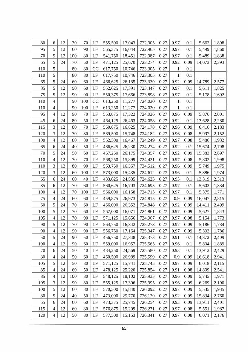
65
80 6 12 70 70 LF 555,500 17,043 722,905 0.27 0.97 0.1 5,662 1,898
95 5 12 60 90 LF 565,375 16,044 722,965 0.27 0.97 0.1 5,499 1,860
70 5 12 100 80 LF 541,750 18,451 722,987 0.27 0.97 0.1 5,489 1,838
65 5 24 70 50 LF 471,125 25,670 723,274 0.27 0.92 0.09 14,073 2,393
110 5 80 80 CC 617,750 10,746 723,305 0.27 1 0.1
110 5 80 80 LF 617,750 10,746 723,305 0.27 1 0.1
65 5 24 60 60 LF 466,625 26,135 723,339 0.27 0.92 0.09 14,789 2,577
85 5 12 90 60 LF 552,625 17,391 723,447 0.27 0.97 0.1 5,611 1,825
75 5 12 90 90 LF 550,375 17,666 723,898 0.27 0.97 0.1 5,178 1,692
110 4 90 100 CC 613,250 11,277 724,020 0.27 1 0.1
110 4 90 100 LF 613,250 11,277 724,020 0.27 1 0.1
95 4 12 90 70 LF 553,875 17,322 724,026 0.27 0.96 0.09 5,876 2,001
45 6 24 80 50 LF 464,125 26,463 724,058 0.27 0.92 0.1 13,628 2,280
115 3 12 80 70 LF 560,875 16,625 724,178 0.27 0.96 0.09 6,416 2,183
120 3 12 70 80 LF 569,500 15,748 724,182 0.27 0.96 0.08 5,997 2,152
100 4 12 80 80 LF 562,500 16,467 724,249 0.27 0.97 0.08 5,486 1,932
65 6 24 40 50 LF 466,625 26,230 724,274 0.27 0.92 0.1 15,674 2,708
70 5 24 50 60 LF 467,250 26,175 724,357 0.27 0.92 0.09 15,383 2,697
110 4 12 70 70 LF 568,250 15,899 724,421 0.27 0.97 0.08 5,802 1,998
110 3 12 80 90 LF 563,750 16,367 724,512 0.27 0.96 0.09 5,749 1,975
120 3 12 60 100 LF 573,000 15,435 724,612 0.27 0.96 0.1 5,886 1,974
65 6 24 60 40 LF 483,625 24,535 724,623 0.27 0.93 0.1 13,319 2,313
85 6 12 70 60 LF 560,625 16,703 724,695 0.27 0.97 0.1 5,603 1,834
100 4 12 70 100 LF 566,000 16,158 724,715 0.27 0.97 0.1 5,375 1,771
75 4 24 60 60 LF 459,875 26,973 724,815 0.27 0.9 0.09 16,047 2,815
60 5 24 70 60 LF 466,000 26,352 724,848 0.27 0.92 0.09 14,411 2,499
100 5 12 70 60 LF 567,000 16,071 724,861 0.27 0.97 0.09 5,627 1,843
105 4 12 70 90 LF 571,125 15,656 724,907 0.27 0.97 0.08 5,154 1,773
90 5 12 70 90 LF 564,750 16,342 725,273 0.27 0.97 0.09 5,186 1,734
90 4 12 90 90 LF 556,750 17,164 725,347 0.27 0.97 0.09 5,303 1,786
50 5 24 90 50 LF 456,750 27,348 725,373 0.27 0.91 0.1 14,372 2,409
100 4 12 90 60 LF 559,000 16,957 725,565 0.27 0.96 0.1 5,804 1,889
70 6 24 50 40 LF 484,250 24,569 725,580 0.27 0.93 0.1 13,912 2,429
80 4 24 50 60 LF 460,500 26,989 725,599 0.27 0.9 0.09 16,618 2,941
105 5 12 50 80 LF 571,125 15,741 725,745 0.27 0.97 0.09 6,018 2,115
85 4 24 60 50 LF 478,125 25,220 725,854 0.27 0.91 0.08 14,809 2,541
85 4 12 100 80 LF 548,125 18,102 725,935 0.27 0.96 0.09 5,745 1,971
105 3 12 90 80 LF 555,125 17,396 725,995 0.27 0.96 0.09 6,269 2,190
100 5 12 60 80 LF 570,500 15,840 726,092 0.27 0.97 0.09 5,535 1,935
80 5 24 40 50 LF 473,000 25,770 726,129 0.27 0.92 0.09 15,834 2,760
55 6 24 60 60 LF 473,375 25,745 726,254 0.27 0.93 0.09 13,911 2,401
115 4 12 60 80 LF 576,875 15,209 726,271 0.27 0.97 0.08 5,551 1,987
120 4 12 50 80 LF 577,500 15,153 726,341 0.27 0.97 0.08 6,071 2,176
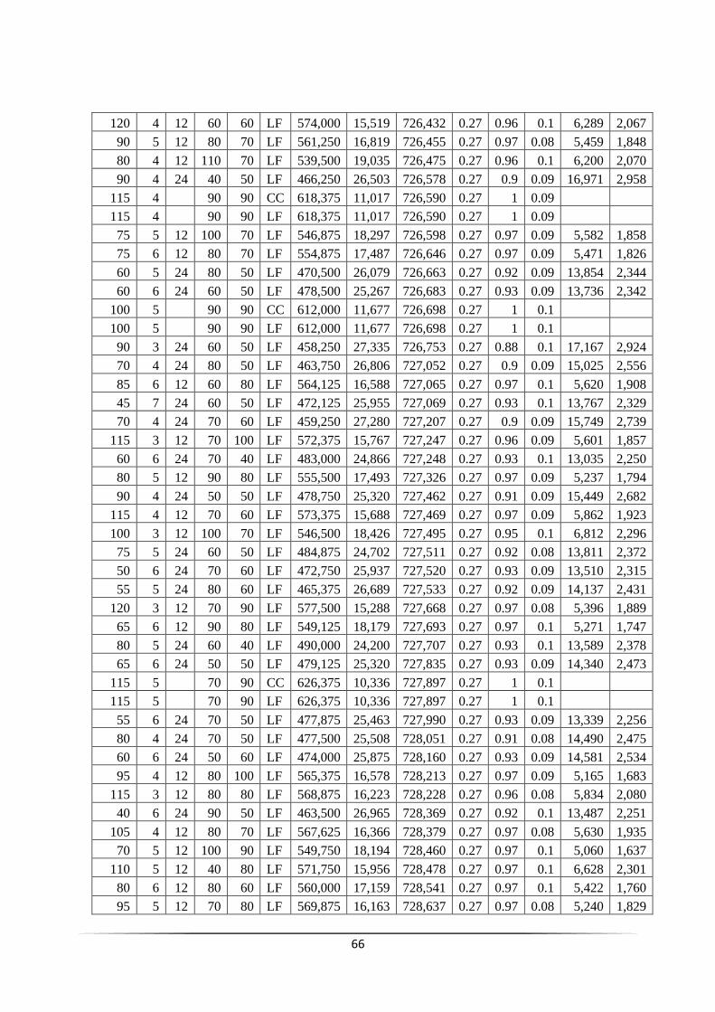
66
120 4 12 60 60 LF 574,000 15,519 726,432 0.27 0.96 0.1 6,289 2,067
90 5 12 80 70 LF 561,250 16,819 726,455 0.27 0.97 0.08 5,459 1,848
80 4 12 110 70 LF 539,500 19,035 726,475 0.27 0.96 0.1 6,200 2,070
90 4 24 40 50 LF 466,250 26,503 726,578 0.27 0.9 0.09 16,971 2,958
115 4 90 90 CC 618,375 11,017 726,590 0.27 1 0.09
115 4 90 90 LF 618,375 11,017 726,590 0.27 1 0.09
75 5 12 100 70 LF 546,875 18,297 726,598 0.27 0.97 0.09 5,582 1,858
75 6 12 80 70 LF 554,875 17,487 726,646 0.27 0.97 0.09 5,471 1,826
60 5 24 80 50 LF 470,500 26,079 726,663 0.27 0.92 0.09 13,854 2,344
60 6 24 60 50 LF 478,500 25,267 726,683 0.27 0.93 0.09 13,736 2,342
100 5 90 90 CC 612,000 11,677 726,698 0.27 1 0.1
100 5 90 90 LF 612,000 11,677 726,698 0.27 1 0.1
90 3 24 60 50 LF 458,250 27,335 726,753 0.27 0.88 0.1 17,167 2,924
70 4 24 80 50 LF 463,750 26,806 727,052 0.27 0.9 0.09 15,025 2,556
85 6 12 60 80 LF 564,125 16,588 727,065 0.27 0.97 0.1 5,620 1,908
45 7 24 60 50 LF 472,125 25,955 727,069 0.27 0.93 0.1 13,767 2,329
70 4 24 70 60 LF 459,250 27,280 727,207 0.27 0.9 0.09 15,749 2,739
115 3 12 70 100 LF 572,375 15,767 727,247 0.27 0.96 0.09 5,601 1,857
60 6 24 70 40 LF 483,000 24,866 727,248 0.27 0.93 0.1 13,035 2,250
80 5 12 90 80 LF 555,500 17,493 727,326 0.27 0.97 0.09 5,237 1,794
90 4 24 50 50 LF 478,750 25,320 727,462 0.27 0.91 0.09 15,449 2,682
115 4 12 70 60 LF 573,375 15,688 727,469 0.27 0.97 0.09 5,862 1,923
100 3 12 100 70 LF 546,500 18,426 727,495 0.27 0.95 0.1 6,812 2,296
75 5 24 60 50 LF 484,875 24,702 727,511 0.27 0.92 0.08 13,811 2,372
50 6 24 70 60 LF 472,750 25,937 727,520 0.27 0.93 0.09 13,510 2,315
55 5 24 80 60 LF 465,375 26,689 727,533 0.27 0.92 0.09 14,137 2,431
120 3 12 70 90 LF 577,500 15,288 727,668 0.27 0.97 0.08 5,396 1,889
65 6 12 90 80 LF 549,125 18,179 727,693 0.27 0.97 0.1 5,271 1,747
80 5 24 60 40 LF 490,000 24,200 727,707 0.27 0.93 0.1 13,589 2,378
65 6 24 50 50 LF 479,125 25,320 727,835 0.27 0.93 0.09 14,340 2,473
115 5 70 90 CC 626,375 10,336 727,897 0.27 1 0.1
115 5 70 90 LF 626,375 10,336 727,897 0.27 1 0.1
55 6 24 70 50 LF 477,875 25,463 727,990 0.27 0.93 0.09 13,339 2,256
80 4 24 70 50 LF 477,500 25,508 728,051 0.27 0.91 0.08 14,490 2,475
60 6 24 50 60 LF 474,000 25,875 728,160 0.27 0.93 0.09 14,581 2,534
95 4 12 80 100 LF 565,375 16,578 728,213 0.27 0.97 0.09 5,165 1,683
115 3 12 80 80 LF 568,875 16,223 728,228 0.27 0.96 0.08 5,834 2,080
40 6 24 90 50 LF 463,500 26,965 728,369 0.27 0.92 0.1 13,487 2,251
105 4 12 80 70 LF 567,625 16,366 728,379 0.27 0.97 0.08 5,630 1,935
70 5 12 100 90 LF 549,750 18,194 728,460 0.27 0.97 0.1 5,060 1,637
110 5 12 40 80 LF 571,750 15,956 728,478 0.27 0.97 0.1 6,628 2,301
80 6 12 80 60 LF 560,000 17,159 728,541 0.27 0.97 0.1 5,422 1,760
95 5 12 70 80 LF 569,875 16,163 728,637 0.27 0.97 0.08 5,240 1,829
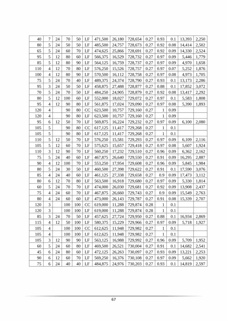
67
40 7 24 70 50 LF 471,500 26,180 728,654 0.27 0.93 0.1 13,393 2,250
80 5 24 50 50 LF 485,500 24,757 728,673 0.27 0.92 0.08 14,414 2,502
65 5 24 60 70 LF 474,625 25,866 728,691 0.27 0.92 0.09 14,330 2,524
95 5 12 80 60 LF 566,375 16,529 728,732 0.27 0.97 0.09 5,446 1,779
85 5 12 80 90 LF 564,125 16,759 728,737 0.27 0.97 0.09 4,970 1,658
110 4 12 70 80 LF 576,250 15,526 728,757 0.27 0.97 0.07 5,252 1,876
100 4 12 80 90 LF 570,500 16,112 728,758 0.27 0.97 0.08 4,973 1,705
75 5 24 70 40 LF 489,375 24,374 728,790 0.27 0.93 0.1 13,173 2,286
95 3 24 50 50 LF 458,875 27,488 728,877 0.27 0.88 0.1 17,852 3,072
70 5 24 70 50 LF 484,250 24,905 728,879 0.27 0.92 0.08 13,417 2,292
80 5 12 100 60 LF 552,000 18,027 729,072 0.27 0.97 0.1 5,583 1,808
95 4 12 90 80 LF 561,875 17,024 729,090 0.27 0.97 0.08 5,390 1,893
120 4 90 80 CC 623,500 10,757 729,160 0.27 1 0.09
120 4 90 80 LF 623,500 10,757 729,160 0.27 1 0.09
95 6 12 50 70 LF 569,875 16,224 729,232 0.27 0.97 0.09 6,100 2,080
105 5 90 80 CC 617,125 11,417 729,268 0.27 1 0.1
105 5 90 80 LF 617,125 11,417 729,268 0.27 1 0.1
110 5 12 50 70 LF 576,250 15,581 729,293 0.27 0.97 0.09 6,109 2,116
105 5 12 60 70 LF 575,625 15,657 729,418 0.27 0.97 0.08 5,607 1,924
110 3 12 90 70 LF 560,250 17,232 729,510 0.27 0.96 0.09 6,362 2,162
75 5 24 40 60 LF 467,875 26,640 729,550 0.27 0.91 0.09 16,295 2,887
90 4 12 100 70 LF 553,250 17,954 729,608 0.27 0.96 0.09 5,845 1,984
80 5 24 30 50 LF 460,500 27,398 729,622 0.27 0.91 0.1 17,590 3,076
85 4 24 40 60 LF 461,125 27,338 729,658 0.27 0.9 0.09 17,473 3,112
80 6 12 70 80 LF 563,500 16,918 729,680 0.27 0.97 0.09 5,330 1,814
60 5 24 70 70 LF 474,000 26,030 729,681 0.27 0.92 0.09 13,908 2,437
75 4 24 60 70 LF 467,875 26,660 729,743 0.27 0.9 0.09 15,549 2,763
80 4 24 60 60 LF 473,000 26,143 729,787 0.27 0.91 0.08 15,339 2,707
120 3 100 100 CC 619,000 11,288 729,874 0.28 1 0.1
120 3 100 100 LF 619,000 11,288 729,874 0.28 1 0.1
85 3 24 70 50 LF 457,625 27,724 729,950 0.27 0.88 0.1 16,934 2,869
115 4 12 50 100 LF 580,375 15,229 729,966 0.27 0.97 0.09 5,718 1,927
105 4 100 100 CC 612,625 11,948 729,982 0.27 1 0.1
105 4 100 100 LF 612,625 11,948 729,982 0.27 1 0.1
105 3 12 90 90 LF 563,125 16,988 729,992 0.27 0.96 0.09 5,709 1,952
60 5 24 60 80 LF 469,500 26,521 730,004 0.27 0.91 0.1 14,682 2,541
45 6 24 80 60 LF 472,125 26,263 730,097 0.27 0.93 0.09 13,221 2,253
90 6 12 60 70 LF 569,250 16,376 730,108 0.27 0.97 0.09 5,662 1,920
75 6 24 40 40 LF 484,875 24,976 730,203 0.27 0.93 0.1 14,819 2,597
68
References
[1].Invest in Ethiopia, Ethiopia trade and investment.
www.ethioembassy.org.uk/trade_and_investment. January 2012
[2].Ethiopian Television (ETV) news. http://www.erta.gov.et January 2012
[3].Bekele G. (2009) “The Study into the Potential and Feasibility of Standalone Solar-Wind Hybrid
Electric Energy Supply System for Application in Ethiopia”, KTH-Royal Institute of Technology
Doctoral Thesis.
[4].Salwan S. Dihrab*, K. Sopian. (2010). Electricity generation of hybrid PV/wind systems in Iraq.
Malaysia: University Kebangsaan Malaysia
[5].Soteris Kalogirou. Solar energy engineering: processes and systems, 1st edn.
[6].Timur Gül (2004).Integrated Analysis of Hybrid Systems for Rural Electrification in Developing
Countries, Stockholm.
[7].J.F. Manwell, J.G. McGowan and A.L. Rogers (2002). Wind energy explained theory, design and
application. University of Massachusetts, Amherst, USA.
[8].C. Dennis Barley, Debra J. Lew1, and Lawrence T. (1997). Sizing wind/ PV hybrids for
households in Inner Mongolia. Austin: Texas Ethiopian Television (ETV) news.
http://www.erta.gov.et January 2012
[9]. HOMER, The Optimization Model for Distributed Power: http://www.nrel.gov/homer
[10].Prof. Antonio Ficarella. A current and future state of art development of hybrid energy system
using wind and PV- solar. Rollo Dario
[11].Duffie J.A., Beckman W.A. (1991) “Solar Engineering of Thermal Processes”, 3rd
Edn. Wiley,
New York,
[12].Frank Fiedler, Victor Pazmino, Irati Berruezo, Victor Maison. PV-wind hybrid systems for
Swedish locations. Högskolan Dalarna: Borlänge
[13].M. Muralikrishna1 and V. Lakshminarayana, (2008). Hybrid (solar and wind) energy systems
for rural electrification. Kilakarai, Tamil Nadu, India, vol. 3, no. 5
[14].S. Diaf 1*, D. Diaf, M. Belhamel, M. Haddadi, A. Louche. A methodology for optimal sizing
of autonomous hybrid PV/wind system. France: Ajaccio
[15].Ethiopian National Metreological Agency
[16].Drake F. and, Mulugetta Y. (1996) “Assessment of solar and wind energy in Ethiopia. I. Solar
energy”, Solar Energy, Vol. 57, No. 3, pp. 205-217
69
[17].Mulugetta Y. and Drake F. (1996) “Assessment of solar and wind energy resources in Ethiopia:
II. Wind energy”, Solar Energy, Vol. 57, No. 4, pp. 323-334
[18].http://en.wikipedia.org
[19].Ethiopia news / GTZ Staff Magazine/August2010.
www.enervest.de/fileadmin/downloads/gtz060810. January 2012
[20].Getachew Asaye. EEPCo Human Power Training and Development. Over Head Distribution
Training 2011/12
[21].http://www.alibaba.com/products/denyo_generator_with_ATS/--410402.html. January 2012
[22].http://www.tradingeconomics.com/ethiopia/population-growth-annual-percent-wb-data.html
[23].http://www.tradingeconomics.com/ethiopia/rural-population-percent-of-total-population-wb-
data.html
[24].http://www.lorentz.de/[email protected] 18 Jan 2012
[25].A. S. Pabla ”Electric power distribution”, 6th edition, Tata McGraw Hill Edition Private
Limited, New Delhi
[26].Wind Power to be Competitive with Natural Gas by 2016 Monday 14 November 2011.
http://oilprice.com/Alternative-Energy/Wind-Power/Wind-Power-To-Be-Competitive-With-
Natural-Gas-By-2016.html. January 2012
[27].Renewable 2011 global report, version2.0/07/2011. http://www.ren21.net
[28].Hardy diesel generators. http://www.hardydiesel.com/diesel-generators-7-33-kw.html. January
2012

70


