Solving the Cell Suppression Problem on Tabular Data with Linear Constraints

Solving the Cell Suppression Problem on

Tabular Data with Linear Constraints

Matteo Fischetti • Juan José SalazarDEI, University of Padova, Italy

DEIOC, University of La Laguna, [email protected] • [email protected]

Cell suppression is a widely used technique for protecting sensitive information in statis-

tical data presented in tabular form. Previous works on the subject mainly concentrate

on 2- and 3-dimensional tables whose entries are subject to marginal totals. In this paper

we address the problem of protecting sensitive data in a statistical table whose entries are

linked by a generic system of linear constraints. This very general setting covers, among

others, k-dimensional tables with marginals as well as the so-called hierarchical and linkedtables that are very often used nowadays for disseminating statistical data. In particular,

we address the optimization problem known in the literature as the (secondary) Cell Sup-

pression Problem, in which the information loss due to suppression has to be minimized.

We introduce a new integer linear programming model and outline an enumerative algo-

rithm for its exact solution. The algorithm can also be used as a heuristic procedure to find

near-optimal solutions. Extensive computational results on a test-bed of 1,160 real-world and

randomly generated instances are presented, showing the effectiveness of the approach. In

particular, we were able to solve to proven optimality 4-dimensional tables with marginals

as well as linked tables of reasonable size (to our knowledge, tables of this kind were never

solved optimally by previous authors).

(Statistical Disclosure Control; Confidentiality; Cell Suppression; Integer Linear Programming;Tabular Data; Branch-and-Cut Algorithms)

1. IntroductionA statistical agency collects data obtained from indi-

vidual respondents. This data is usually obtained

under a pledge of confidentiality, i.e., statistical agen-

cies cannot release any data or data summaries

from which individual respondent information can be

revealed (sensitive data). On the other hand, statistical

agencies aim at publishing as much information as

possible, which results in a trade-off between privacy

rights and information loss. This is an issue of pri-

mary importance in practice; see, e.g., Willenborg and

De Wall (1996) for an in-depth analysis of statistical

disclosure control methodologies.

Cell suppression is a widely used technique for

disclosure avoidance. We will introduce the basic

cell suppression problem with the help of a simple

example taken from Willenborg and De Wall (1996).

Figure 1(a) exhibits a 2-dimensional statistical table

giving the investment of enterprises (per millions of

guilders), classified by activity and region. Let us

assume that the information in the cell (2,3)—the one

corresponding to Activity II and Region C—is con-

sidered confidential by the statistical office, according

to a certain criterion (as discussed, e.g., in Willenborg

and De Wall 1996), hence it is viewed as a sensitivecell to be suppressed (primary suppression). But that isnot enough: By using the marginal totals, an attackerinterested in the disclosure of the sensitive cell can

easily recompute its missing value. Then other table

entries cannot be published as well (complementary

Management Science © 2001 INFORMSVol. 47, No. 7, July 2001 pp. 1008–1027

0025-1909/01/4707/1008$5.001526-5501 electronic ISSN

FISCHETTI AND SALAZARThe Cell Suppression Problem on Tabular Data with Linear Constraints

Figure 1 Investment of Enterprises by Activity and Region

A B C Total

Activity I 20 50 10 80

Activity II 8 19 22 49

Activity III 17 32 12 61

Total 45 101 44 190

(a) Original table

A B C Total

Activity I 20 50 10 80

Activity II * 19 * 49

Activity III * 32 * 61

Total 45 101 44 190

(b) Published table

suppression). For example, with the missing entries in

Figure 1(b), an attacker cannot disclose the nominal

value of the sensitive cell exactly, although he/she can

still compute a range for the values of this cell which

are consistent with the published entries. Indeed, the

minimum value y23for the sensitive cell can be com-

puted by solving a linear program in which the values

yij for the missing cells �i� j� are treated as unknowns,

namely

y23�=min y23�

subject to

y21 +y23 = 30

y31 +y33 = 29

y21 +y31 = 25

y23 +y33 = 34

y21� y31� y23� y33 ≥ 0�

Notice that the right-hand side values are known to

the attacker, as they can be obtained as the difference

between the marginal and the published values in a

row/column.

The maximum value y23

for the sensitive cell can

be computed in a perfectly analogous way, by solving

the linear program of maximizing y23 subject to the

same constraints as before.

In the example, y23

= 5 and y23

= 30, i.e., the

sensitive information is “protected” within the pro-tection inverval [5, 30]. If this interval is considered

sufficiently wide by the statistical office, the sensitive

cell is called protected; otherwise new suppressions are

needed. (Notice that the extreme values of interval

[5, 30] are only attained if the cell corresponding to

Activity II and Region A takes the quite unreason-

able values of 0 and 25; bounding the cell variation to

±50% of the nominal value (say) results in the more

realistic protection interval [18, 26].)

The Cell Suppression Problem (CSP) consists of find-

ing a set of cells whose suppression guarantees the

protection of all the sensitive cells against the attacker,

with minimum loss of information associated with

the suppressed entries. This problem belongs to the

class of the strongly ��-hard problems (see, e.g.,

Kelly et al. 1992, Geurts 1992, Kao 1996), meaning

that it is very unlikely that an algorithm for the exact

solution of CSP exists, which guarantees an efficient

(polynomial-time) performance for all possible input

instances.

Previous works on CSP mainly concentrate on

heuristic algorithms for 2-dimensional tables with

marginals, see Cox (1980, 1995), Sande (1984), Kelly

et al. (1992), and Carvalho et al. (1994), among oth-

ers. Kelly (1990) proposed a mixed-integer linear pro-

graming formulation for 2- and 3-dimensional tables

with marginals, which requires a very large num-

ber of variables and constraints. Geurts (1992) refined

the 2-dimensional model slightly, and reported com-

putational experiences on small-size instances, the

largest instance solved to optimality being a table

with 20 rows, 6 columns, and 17 sensitive cells.

Gusfield (1988) gave a polynomial-time algorithm for

a special case of the problem in 2-dimensional tables.

Recently, we presented in Fischetti and Salazar (1999)

a new method capable of solving to proven optimality

2-dimensional instances with up to 250,000 cells and

10,000 sensitive cells on a personal computer.

Heuristics for 3-dimensional tables with marginals

have been proposed in Robertson (1995), Sande

(1984), and Dellaert and Luijten (1996).

In this paper we address the problem of pro-

tecting sensitive data in a statistical table whose

entries are linked by a generic system of linear equa-

tions. This very general setting covers, among others,

k-dimensional tables with marginals, as well as the

so-called hierarchical and linked tables.

Management Science/Vol. 47, No. 7, July 2001 1009


Hierarchical and linked tables consist of a set of

k-dimensional tables derived from a common dataset.

These structures became more and more important in

the recent years, as the technology today allows for

electronic dissemination of large collections of statis-

tical data-sets. As discussed, e.g., in Willenborg and

de Wall (1996), the intrinsic complexity of hierar-

chical and linked tables calls for updated disclosure

control methodologies. Indeed, the individual protec-

tion of each table belonging to a hierarchical/linked

set is not guaranteed to produce safe results. For

example, Sande (1998) showed how it is possible to

disclose confidential information by means of linear

programming methods applied to statistical surveys

recently published by credited statistical offices. This

gave us motivation to improve the current under-

standing of the cell suppression problem for complex

data structures. Unfortunately, the extension from

2-dimensional tables to hierarchical/linked tables is

far from trivial. In particular, the nice network struc-

ture we exploited in Fischetti and Salazar (1999) for

addressing 2-dimensional tables does not extend to

the general case, hence the study of the general setting

needs more sophisticated mathematical and algorith-

mic tools (e.g., Benders’ decomposition instead of the

classical max-flow/min-cut theorem).

The paper is organized as follows. A formal

description of the cell suppression problem is given

in §2. Section 3 introduces and discusses new math-

ematical models for the problem. In particular, a

new integer linear programming model is proposed,

having a 0-1 decision variable for each potential sup-

pression and an exponential number of linear con-

straints enforcing the protection level requirements.

Section 4 addresses efficient methods for solving the

proposed model within the so-called branch-and-cut

framework. Section 5 illustrates our solution method

through a simple example. Computational results are

given in §6, where nine real-world instances are opti-

mally solved on a PC within acceptable computing

time. In particular, we were able to solve to proven

optimality a 4-dimensional table with marginals and

four linked tables. Extensive computational results on

1,160 randomly generated 3- and 4-dimensional tables

are also reported. Some conclusions are finally drawn

in §7.

2. The Cell Suppression ProblemWe next give a formal definition of the cell suppres-

sion problem we address in this paper.

A table is a vector y= �y1 · · ·yn� whose entries satisfya given set of linear constraints known to a possible

attacker, namely

My = b

lbi ≤ yi ≤ ubi for all i = 1� � � � �n�

}� (1)

In other words, system (1) models the whole a priori

information on the table known to an attacker. Typi-

cally, each equation in (1) corresponds to a marginal

entry, whereas inequalities enforce the “external

bounds” known to the attacker.

In the case of k-dimensional tables with marginals,

each equation in (1) is of the type∑

j∈Qiyj − yi = 0,

where index i corresponds to a marginal entry and

index set Qi to the associated internal table entries.

Therefore, in this case M is a �0�±1-matrix and

b = 0. Moreover, in case k = 2, the linear system (1)

can be represented in a natural way as a network,a property having important theoretical and prac-

tical implications; see, e.g., Cox (1980, 1995), Kelly

et al. (1992), and Fischetti and Salazar (1999). Unfor-

tunately, this nice structure is not preserved for k ≥ 3,

unless the table decomposes into a set of independent

2-dimensional subtables.

A cell is an index corresponding to an entry of the

table.

Given a nominal table a, let PS = �i1� � � � � ip be

the set of sensitive cells to be protected, as identi-

fied by the statistical office according to some criteria.

For each sensitive cell ik �k = 1� � � � � p�, the statisti-

cal office provides three nonnegative values, namely

LPLk�UPLk, and SPLk, called Lower Protection Level,Upper Protection Level, and Sliding Protection Level,respectively, whose role will be discussed next. In typ-

ical applications, these values are computed as a cer-

tain percentage of the nominal value aik .

A suppression pattern is a subset of cells SUP ⊆�1� � � � �n corresponding to the unpublished cells. A

consistent table with respect to a given suppression

1010 Management Science/Vol. 47, No. 7, July 2001


pattern SUP and to a given nominal table a is a vectory = �y1 · · ·yn� satisfying

My = b

lbi ≤ yi ≤ ubi for all i ∈ SUP

yi = ai for all i �∈ SUP

� (2)

where the latter equations impose that the com-

ponents of y associated with the published entries

coincide with the nominal ones. In other words, any

consistent table gives a feasible way the attacker can

fill the missing entries of the published table.

A suppression pattern is considered feasible by the

statistical office if it guarantees the required protec-

tion intervals against an attacker, in the sense that,

for each sensitive cell ik �k= 1� � � � � p�, there exist twoconsistent tables, say f k and gk, such that

f kik≤ aik −LPLk� gkik ≥ aik +UPLk�

and gkik −f kik≥ SPLk� (3)

In other words, it is required that yik≤ aik −LPLk� yik ≥

aik +UPLk, and yik −yik≥ SPLk, where

yik �= max�yik � �2� holds and

yik�= min�yik � �2� holds�

Note that each nonzero sliding protection level

SPLk allows the statistical office to control the length

of the uncertainty range for cell k without forcing spe-cific upper and lower bounds UPLk and LPLk (theselatter bounds being typically set to zero in case SLPk �=0), a situation which is sometimes preferred to reduce

the potential correlation of the unpublished “true”

value aik with the attacker “middle-point” estimate

�yik +yik�/2.

As already mentioned, the statistical office is inter-

ested in selecting, among all feasible suppression pat-

terns, a one with minimum information loss. This

issue can be modeled by associating a weight wi ≥0 with each entry of the table, and by requiring

the minimization of the overall weight of the sup-

pressed cells, namely∑

i∈SUP wi. In typical applica-

tions, the weights wi provided by the statistical office

are proportional to ai or to log�ai�. The resulting

combinatorial problem is known in the literature as

the (complementary or secondary) Cell SuppressionProblem, or CSP for short.

3. A New Integer LinearProgramming Model

In the sequel, for notational convenience we define

the relative external bounds:

LBi �= ai− lbi ≥ 0 and UBi �= ubi−ai ≥ 0�

i.e., the range of feasible values for cell i known to the

attacker is �ai−LBi� ai+UBi�.To obtain a Mixed-Integer Linear Programming

(MILP) model for CSP, we introduce a binary variable

xi = 1 for each cell i, where xi = 1 if i ∈ SUP (sup-

pressed), and xi = 0 otherwise (published). Clearly, we

can fix xi = 0 for all cells that have to be published (if

any), and xi = 1 for all cells that have to be suppressed

(sensitive cells). Using this set of variables, the model

is of the form

minn∑i=1

wixi (4)

subject to x ∈ �0�1n and, for each sensitive cell ik �k=1� � � � � p�:

The suppression pattern associated

with x satisfies the lower protection

level requirement with respect to cell ik

� (5)

the suppression pattern associated

with x satisfies the upper protection


� (6)

the suppression pattern associated

with x satisfies the sliding protection


� (7)

3.1. The Classical ModelA possible way to express Conditions (5)–(7) through

linear constraints requires the introduction, for each

k = 1� � � � � p, of auxiliary continuous variables f k =[f ki � i = 1� � � � �n

]and gk = [

gki � i = 1� � � � �n]defin-

ing tables that are consistent with respect to the sup-

pression pattern associated with x and satisfy (3).

This is in the spirit of the MILP model proposed by

Kelly (1990) for 2-dimensional tables with marginals.

The resulting MILP model then reads:

minn∑i=1

wixi� (8)



subject to x ∈ �0�1n and, for each sensitive cell ik �k=1� � � � � p�:

Mfk = b

ai−LBixi ≤ f ki ≤ ai+UBixi for i = 1� � � � �n

}� (9)

Mgk = b

ai−LBixi ≤ gki ≤ ai+UBixi for i = 1� � � � �n

}� (10)

f kik≤ aik −LPLk� (11)

gkik ≥ aik +UPLk� (12)

gkik −f kik≥ SPLk� (13)

Notice that the lower/upper bounds on the vari-

ables f ki and gki in (9) and (10) depend on xi so as to

enforce f ki = gki = ai whenever xi = 0 (cell i is not sup-

pressed), and lbi ≤ f ki ≤ubi and lbi ≤ gki ≤ubi otherwise

(cell i is suppressed). Therefore, (9) and (10) stipu-

late the consistency of f k and gk, respectively, with

the published table, whereas (11), (12), and (13) trans-

late the protection level requirements (5), (6), and (7),

respectively.

Standard MILP solution techniques such as branch-

and-bound or cutting-plane methods (see, e.g.,

Nemhauser and Wolsey 1988) require the solution of

the Linear Programming (LP) relaxation of the model

in hand, obtained by relaxing conditions xi ∈ �0�1

into 0 ≤ xi ≤ 1 for all i. However, even the LP relax-

ation of Model (8)–(13) is very difficult to solve in

that it involves a really huge number of auxiliary vari-

ables f ki and gki and linking constraints between the x

and the auxiliary variables. For example, for a 100×100 table with marginals having 5% sensitive cells,

the model needs more than 10,000,000 variables and

20,000,000 constraints—a size that cannot be handled

explicitly by the today LP technology.

We next propose a new model based on Benders’

decomposition (see e.g. Nemhauser and Wolsey 1988).

The idea is to use standard LP duality theory to

avoid the introduction of the auxiliary variables f k

and gk �k = 1� � � � � p� along with the associated link-

ing constraints. In the new model, the protection level

requirements are in fact imposed by means of a fam-

ily of linear constraints in the space of the x-variables

only. Before formulating the new model, we need a

characterization of the vectors x for which Systems

(9)–(13) admit feasible f k and gk solutions, which is

obtained as follows.

3.2. Imposing the Upper ProtectionLevel Requirements

Assume that x is a given (arbitrary but fixed) param-

eter, and consider any given sensitive cell ik �k =1� � � � � p� along with the associated upper protec-

tion level requirement. Clearly, the linear system (10)

and (12) admits a feasible solution gk if and only

if aik +UPL ≤ yik , where yik is the optimal value of

the linear problem

yik �=maxyik� (14)

subject to

My = b� (15)

yi ≤ ai+UBixi for all i = 1� � � � �n� (16)

−yi ≤ −ai+LBixi for all i = 1� � � � �n� (17)

This is a parametric LP problem in the y-variablesonly, with variable upper/lower bounds depending

on the given parameter x. We call (14)–(17) the attackersubproblem associated with the upper protection of

sensitive cell ik, with respect to parameter x. By LP

duality, this subproblem is equivalent to the linear

problem

yik = mintb+n∑i=1

(�i�ai+UBixi�−�i�ai−LBixi�

)� (18)

subject to

�t−�t+tM = etik�≥ 0��≥ 0� unrestricted in sign

}� (19)

where eik denotes the ikth column of the identify

matrix of order n, and ��, and � are the dual vec-

tors associated with constraints (15), (16), and (17),

respectively.

It then follows that the linear system (10) and (12)

has a feasible solution if and only if

aik +UPLk ≤ yik = min

{tb+

n∑i=1

(�i�ai+UBixi�

−�i�ai−LBixi�)� �19� holds

}�



i.e., if and only if

aik +UPLk ≤ tb+n∑i=1


)for all �� satisfying �19��

Because of (19) and Ma = b, we have tb +∑ni=1��iai−�iai�= tMa+ ��−��ta= etika= aik . Hence

the above system can be rewritten as

n∑i=1��iUBi+�iLBi�xi ≥ UPLk�

for all �� satisfying �19�� (20)

In other words, System (20) defines a set of con-

straints, in the x variables only, which is equivalent to

Condition (6) concerning the upper protection level

requirement for sensitive cell ik.

Notice that (20) contains in principle an infinite

number of constraints, each associated with a dif-

ferent point �� of the polyhedron defined by

(19). However, it is well known (see, e.g., Nemhauser

and Wolsey 1988) that only the extreme points (and

rays) of such polyhedron can lead to nondominated

constraints (20), i.e., a finite number of such con-

straints is sufficient to impose the upper protection

level requirement for a given sensitive cell ik.

3.3. Imposing the Lower ProtectionLevel Requirements

Analogously, the lower protection level requirement

for a given cell ik is equivalent to imposing yik≤ aik −

LPLk, where

yik�= min�yik � �15�−�17� hold≡ −max�−yik � �15�−�17� hold� (21)

This is called the attacker subproblem associated to the

lower protection of sensitive cell ik, with respect to

parameter x. By LP duality, this subproblem is equiv-

alent to the linear problem

yik=mintb+

n∑i=1


)�

(22)

subject to

�t−�t+tM =−etik�≥ 0��≥ 0� unrestricted in sign.

}� (23)

Hence the lower protection level requirement (5) for

cell ik can be formulated as

aik −LPLk ≥ −(tb+

n∑i=1

(�i�ai+UBixi�

−�i�ai−LBixi�))

for all �� satisfying (23),

or, equivalently,

n∑i=1��iUBi+�iLBi�xi ≥ LPLk

for all �� satisfying (23).

3.4. Imposing the Sliding ProtectionLevel Requirements

As to the sliding protection level for sensitive cell ik,

the requirement is that

SPLk ≤ yik −yik�= max�yik � (15)–(17) hold

+ max�−yik � (15)–(17) hold�

Again, by LP duality, this condition is equivalent to

SPLk ≤ max

{tb+

n∑i=1

(�i�ai+UBixi�


}

+ max

{tb+

n∑i=1

(�i�ai+UBixi�


}�

Therefore, the feasibility condition can now be formu-

lated by requiring

SPLk ≤ �+ ′�tb+n∑i=1

(��i+�′

i��ai+UBixi�

− ��i+�′i��ai−LBixi�

)for all �� satisfying (19) and for all

�′��′� ′ satisfying (23),



or, equivalently,

n∑i=1

(��i+�′

i�UBi+ ��i+�′i�LBi

)xi ≥ SPLk

for all �� satisfying (19) and for all �′��′� ′

satisfying (23).

3.5. The New ModelThe above characterization of the feasible vectors xleads to the following new integer linear model for

CSP:

minn∑i=1

wixi (24)

subject to x ∈ �0�1n and, for each sensitive cell ik �k=1� � � � � p�:∑n

i=1��iUBi+�iLBi�xi ≥ UPLkfor all extreme points ��

satisfying (19)

� (25)

∑ni=1��iUBi+�iLBi�xi ≥ LPLkfor all extreme points ��

satisfying (23)

� (26)

∑ni=1

(��i+�′

i�UBi+ ��i+�′i�LBi

)xi ≥ SPLk

for all extreme points ��

satisfying (19) and for all extreme

points ��′��′� ′� satisfying (23)

� (27)

Notice that all the left-hand-side coefficients of vari-

ables xi are nonnegative. As a consequence, all the

constraints with zero right-hand-side value need not

to be included in the model, as they do not corre-

spond to a proper protection level requirement.

We call (25)–(27) the capacity constraints in analogy

with similar constraints we introduced in Fischetti

and Salazar (1999) for 2-dimensional tables with

marginals for enforcing a sufficient “capacity” of

certain cuts in the network representation of the

problem. Intuitively, the capacity constraints force to

suppress (i.e., to set xi = 1) a sufficient number of cells

whose positions within the table and contributions

to the overall protection are determined by the dual

variables �� of the attacker subproblems.

4. Solving the New ModelThe solution of model (24)–(27) can be achieved

through an enumerative scheme commonly known as

branch-and-cut, as introduced by Padberg and Rinaldi

(1991) (see Caprara and Fischetti 1997 for a recent

annotated bibliography on the subject). The main

ingredients of the scheme are described next.

4.1. Solving the LP RelaxationThe solution of the LP relaxation of Model (24)–(27)

is approached through the following cutting-plane

scheme. We start by solving the so-called master LP

min

{ n∑i=1

wixi � xi1 = · · · = xip = 1�x ∈ �0�1�n}

in which we only impose the suppression of the sen-

sitive cells. Let x∗ be the optimal solution found.

Our order of business is to check whether the vec-

tor x∗ (viewed as a given parameter) guarantees the

required protection levels. In geometrical terms, this

is equivalent to finding an hyperplane in the x-space

that separates x∗ from the polyhedron defined by the

capacity constraints. This is called the separation prob-lem associated with the family of capacity constraints

(25)–(27), and can be solved efficiently as follows.

For each sensitive cell ik, in turn, we apply the fol-

lowing steps:

1. We first solve the attacker subproblem (14)–(17)

for x = x∗ and check whether aik +UPLk ≤ yik . If this

is the case, then x∗ satisfies the upper protection level

requirement for the given ik, hence all the capacity

constraints (25) are certainly fulfilled. Otherwise, the

optimal dual solution �� of the attacker sub-

problem satisfies (19) and

tb+n∑i=1

(�i�ai+UBix

∗i �− �i�ai−LBix

∗i �)

= yik < aik +UPLk�

hence it induces a capacity constraint∑n

i=1(�iUBi +

�iLBi�xi ≥ UPLk in family (25) that is violated by x∗.This constraint is then added to the master LP.

2. We then check whether x∗ satisfies the lower pro-

tection level requirement for ik, which requires the

solution of the attacker subproblem (21) associated

with the lower protection level of cell ik, and possibly

add to the master LP a violated capacity constraint in

family (26).



3. Finally, we check whether x∗ satisfies the slidingprotection level for ik. This simply requires checking

whether the values yik and yikcomputed in the previ-

ous steps satisfy yik −yik≥ SPLk. If this is not the case,

setting �� = �� and ��′��′� ′� �= ��

leads to a violated capacity cut (27).

Clearly, Steps 1 and 3 (respectively, Steps 2 and

3) can be avoided if LPLk = SPLk = 0 (respectively,

UPLk = SPLk = 0).

After having considered all sensitive cells ik we

have two possible cases. If no capacity constraint has

been added to the master LP, then all of them are sat-

isfied by x∗ which is therefore an optimal solution of

the LP relaxation of Model (24)–(27). Otherwise, the

master LP amended by the new capacity constraints

is reoptimized and the approach is iterated on the

(possibly fractional) optimal solution x∗ of the new

master LP.

By using the above cutting-plane scheme one can

solve efficiently the overall LP relaxation of our

model, since the above-described separation proce-

dure for capacity constraints (25)–(27) can be imple-

mented to run in polynomial time.

4.2. Strengthening the LP RelaxationThe effectiveness of the branch-and-cut approach

greatly depends on how tightly the LP relaxation

approximates the integer solution set. In this respect,

adding to the model new classes of linear constraints

can be greatly beneficial, in that the additional con-

straints (which are redundant when the integrality

condition on the variables is active) can produce tight-

ened LP relaxations, and hence a significant speed-up

in the overall problem resolution.

We next outline some families of additional con-

straints that we found effective in our computational

experience. As in the case of capacity constraints,

these new inequalities are added to the LP relax-

ation on the fly, when they are violated by the solu-

tion x∗ of the current master LP. This requires the

exact/heuristic solution of the separation problem

associated with each new family of constraints.

4.2.1. Strengthened Capacity Constraints. Capac-ity constraints have been derived without using the

information on the integrality of the x variables.

Indeed, let

n∑i=1

sixi ≥ s0 (28)

represent any capacity inequality (25)–(27), whose

coefficients s1� � � � � sn are all nonnegative. We claim

that any integer vector x ≥ 0 satisfying (28) must also

satisfy

n∑i=1

min�si� s0xi ≥ s0� (29)

Indeed, let T �= �i ∈ �1� � � � �n � si > s0. Given any inte-

ger x ≥ 0 satisfying (28), if xi = 0 for all i ∈ T then∑ni=1 min�si� s0xi =

∑ni=1 sixi ≥ s0. Otherwise, we have∑n

i=1 min�si� s0xi ≥ s0xj ≥ s0, where j is any index in T

such that xj �= 0 (hence xj ≥ 1).

Notice that Condition (29) is stronger than (28)

when x is not integer, a case of interest when solving

the LP relaxation of our model.

As already discussed, the use of the strengthened

capacity constraints requires to address the associ-

ated separation problem. In our implementation we

use a simple separation heuristic in which we apply

the strengthening procedure only to the capacity con-

straints associated with the optimal dual solutions of

the attacker subproblems, computed as described in

§4.1.

Although very simple, the above improvement is

quite effective in practice, mainly when UPLk�LPLk,

and/or SPLk are small in comparison with the given

external relative bounds UBi and LBis. Indeed, our

computational experience shows that deactivating

this improvement has a dramatic impact on the model

quality, and hence on the convergence properties of

our code.

4.2.2. Cover Inequalities. Following the seminal

work of Crowder et al. (1983) on the solution of gen-

eral integer programming models, we can observe

that each single-capacity inequality implies a number

of “more combinatorial” restrictions. To be specific, let

again∑

i sixi ≥ s0 represent any strengthened capacity

constraints in (29), whose coefficients si are all non-

negative. Clearly, one has to suppress at least one cell

for any subset Q ⊆ �1� � � � �n such that∑

i �∈Q si < s0, a



condition that can be expressed by means of the fol-

lowing cover inequalities:

∑i∈Q

xi ≥ 1� for each cell subset Q �∑i �∈Q

si < s0� (30)

These inequalities can easily be improved to their

lifted form:

∑i∈EXT�Q�

xi ≥ EXT�Q�− Q+1�

for each cell subset Q �∑i �∈Q

si < s0� (31)

where EXT�Q� �=Q∪ �i � si ≥max�sj � j ∈Q. We refer

the interested reader to, e.g., Nemhauser and Wolsey

(1988) for a discussion on the validity of lifted cover

inequalities, and for possible procedures to solve the

associated separation problem.

4.2.3. Bridgeless Inequalities. As the weights wi

are assumed to be nonnegative, every CSP instance

has an optimal solution in which no suppression is

redundant. Therefore, one can require that the value

of each cell with xh = 1 cannot be recomputed exactly.

This is equivalent to associate a very small ficti-

tious sliding protection level > 0 to each suppressed

nonsensitive cell, and to set-up the associated attacker

subproblems with the requirement that

yh−yh≥ xh�

Notice that this condition is only active for sup-

pressed cells h and vanishes when xh = 0.

As already discussed, the above condition on the

optimal values yh and yhof the attacker subproblems

can be enforced by the following class of capacity con-

straints

n∑i=1��i+�′

i�UBi+ ��i+�′i�LBi�xi ≥ xh� (32)

valid for all extreme points �� satisfying (19)

and for all extreme points ��′��′� ′� satisfying (23),

with cell h playing the role of ik. These constraints

are of the same nature as Constraints (27), but have a

zero right-hand-side value when xh = 0.

As stated, Conditions (32) can be very weak, in

that the right-hand-side value is very close to zero.

However, they become effective in their strengthened

form: ∑i∈Q

xi ≥ xh� (33)

where Q �= �i ∈ �1� � � � �n � ��i+�′i�UBi+��i+�′

i�LBi >0, and �� and ��′��′� ′� are as before. We call

(33) the bridgeless inequalities, as in the 2-dimensional

case they forbid the presence of “bridges” in a cer-

tain network structure associated with the suppressed

cells; see Fischetti and Salazar (1999) for details.

The separation problem for bridgeless inequalities

is perfectly analogous to the one described for the

strengthened capacity constraints (sliding case), and

requires the solution of the two attacker subproblems

associated with any nonsensitive cell h with x∗h > 0.

4.3. BranchingWhenever the solution of the LP relaxation of our

strengthened model (say x∗) is noninteger and has

an objective value smaller than the value of the cur-

rent best feasible solution, we branch on a fractional

variable xb chosen according to the following “strong

branching” criterion (see Applegate et al. 1995). We

first identify the 10 fractional variables x∗i that are as

close as possible to 0.5. For each such variable, in

turn, we solve our current LP model amended by the

new condition xi = 0 or xi = 1, so as to estimate the

effect of branching on xi. The actual branching vari-

able xb is then chosen as the one maximizing the aver-

age subproblem lower bound �z0i +z1i �/2, where z0i and

z1i denote the optimal solution values of the two LP

problems associated with condition xi = 0 and xi = 1,

respectively.

4.4. Problem ReductionThe computing time spent in the solution of a given

instance depends on its size, expressed in terms of

both the number of decision variables involved, and

the number of nonzero protection levels (recall that

zero protection levels do not induce capacity con-

straints). We next outline simple criteria to reduce the

size of a given CSP instance.

A (typically substantial) reduction on the number of

nonzero protection levels is achieved in a preprocess-ing phase, to be applied before entering the branch-

and-cut scheme. This is based on the observation that



primary suppressions alone may be sufficient to pro-

tect some of the sensitive cells which therefore do

not need to be considered sensitive anymore. To be

specific, we consider the suppression pattern SUP �=�i1� � � � � ip and for each sensitive cell ik we solve the

attacker subproblem (14)–(17). In case yik ≥ aik +UPLkone can clearly set UPLk = 0, thus deactivating the

upper protection level requirement for ik. Otherwise,the (strengthened) capacity constraint associated with

the dual optimal solution of the attacker subproblem

qualifies as a relevant constraint, hence it is stored in

the branch-and-cut constraint pool. A similar reason-

ing applies to lower and sliding protection levels.

A naive implementation of the above idea may be

excessively time consuming for large instances, in that

it may require even more computing time than the

whole branch-and-cut algorithm applied on the origi-

nal instance. Hence a parametric resolution of the sev-

eral attacker subproblems involved in preprocessing

is needed. We suggest the following approach.

We introduce two p-dimensional arrays HIGH and

LOW, whose entries HIGHk and LOWk give, respec-

tively, lower and upper bounds on the solution

value yik and yikof the attacker subproblems associ-

ated with ik, with respect to the suppression pattern

SUP = �i1� � � � � ip. We initialize HIGHk �= LOWk �=aik for all k = 1� � � � � p and then consider the sensi-

tive cells ik according to a nonincreasing sequence

of the associated values max�SPLk�UPLk+LPLk. Foreach ik, we first check whether HIGHk < aik +UPLkor HIGHk− LOWk < SPLk, in which case we solve

the attacker subproblem (14)–(17) and obtain a con-

sistent table y maximizing yik . The entries of y are

then used to update all the entries of HIGH and LOW

by setting HIGHh = max�HIGHh� yih and LOWh =min�LOWh� yih for all h = 1� � � � � p. We then check

whether LOWk > aik − LPLk or HIGHk− LOWk <SPLk, in which case we solve the attacker subprob-

lem (21) and obtain a consistent table y minimizing

yik . As before, the entries of y are used to update all

the entries of HIGH and LOW. Finally, we use the

updated values HIGHk and LOWk to set UPLk = 0 (if

HIGHk ≥ aik +UPLk��LPLk = 0 (if LOWk ≤ aik −LPLk),and SPLK = 0 (if HIGHk− LOWk ≥ SPLk). In this way

we avoid a (typically substantial) number of attacker

subproblem resolutions.

Whenever a protection level associated to ik is not

satisfied, we have at hand a capacity constraint asso-

ciated with the dual optimal solution of the corre-

sponding attacker subproblem, which can be used to

initialize the constraint pool. In this way, with no

extra computing time we perform both the prepro-

cessing phase and initialize the constraint pool with a

number of relevant constraints.

We now address the reduction of variables in the

LP programs to be solved within our branch-and-

cut algorithm. Our approach is to fix to 0 or 1 some

decision variables during the processing of the cur-

rent node of the branch-decision tree. We use the

classical criteria based on LP reduced cost; see, e.g.,

Nemhauser and Wolsey (1988). According to our com-

putational experience, these criteria allow one to fix

a large percentage of the variables very early during

the computation. Moreover, we have implemented a

variable-pricing technique to speed-up the overall com-

putation and to drastically reduce memory require-

ment when instances with more than 10,000 variables

are considered; see, e.g., Nemhauser and Wolsey

(1988) for details.

4.5. HeuristicThe convergence of the overall branch-and-bound

scheme can be speeded up if a near-optimal CSP

solution is found very early during computation.

Therefore one is interested in an efficient heuristic

algorithm, to be applied (possibly several times) at

each node of the branch-decision tree.

The avaliability of a good heuristic solution is also

important when the convergence of the branch-and-

cut scheme requires large computing time, and one

has to stop the algorithm before convergence.

We have implemented a heuristic procedure in the

spirit of the one proposed by Kelly et al. (1992) and

Robertson (1995). Our procedure works in stages, in

each of which one finds heuristically a set of new

suppressions needed to guarantee the required pro-

tection levels for a certain sensitive cell ik. To be more

specific, we start by defining the current set of sup-

pressions, SUP �= �i1� � � � � ip, and define ci �= 0 for all

i ∈ SUP, and ci �=wi for all i �∈ SUP. Then we consider

all the sensitive cells ik according to some heuristically

defined sequence.



For each such ik, in turn, we first consider the fol-

lowing incremental attacker subproblem associated with

the upper protection level UPLk (if different from 0):

minn∑i=1

ci�y+i +y−

i � (34)

subject to

M�y+−y−�= 0 (35)

0≤ y+i ≤ UBi for all i = 1� � � � �n� (36)

0≤ y−i ≤ LBi for all i = 1� � � � �n� (37)

y−ik= 0 and y+

ik= UPLk� (38)

Variables y+i and y−

i correspond to possible incre-

ments or decrements of value ai in a consistent table

y �= a+ y+ − y−. Constraints (35)–(37) stipulate the

consistency of table y, whereas (38) imposes yik = aik +UPLk. The objective function (34) gives an estimation

of the additional weight associated with the suppres-

sion of the entries i �∈ SUP with yi �= ai (i.e., with y+i +

y−i > 0).

We solve Problem (34)–(38) and insert in SUP all

the cells i �∈ SUP having y+i + y−

i > 0 in the opti-

mal solution. This guarantees the fulfillment of the

upper protection level requirement for ik with respect

to the new set SUP of suppressions. Afterwards, we

set ci = 0 for all i ∈ SUP, and apply a similar tech-

nique to extend SUP to guarantee the fulfillment of

the lower and sliding protection levels. This requires

to solve Model (34)–(38) two additional times, a first

time with (38) replaced by y+ik= 0 and y−

ik= LPLk, and

a second time with (38) replaced by y+ik+y−

ik= SPLk.

As in the problem reduction, a parametric resolu-

tion of the incremental attacker subproblems typically

reduces considerably the computational effort spent

within the heuristic.

In some cases, the above heuristic can introduce

redundant suppressions. Hence it may be worth

applying a clean-up procedure to detect and remove

such redundancies; see, e.g., Kelly et al. (1992). To

this end, let SUP denote the feasible suppression pat-

tern found by the heuristic. The clean-up procedure

considers, in sequence, all the complementary sup-

pressions h∈ SUP\�i1� � � � � ip, according to decreasing

weights wh, and checks whether SUP\�h is a feasi-

ble suppression pattern as well, in which case SUP is

replaced by SUP\�h.Clean up can be very time consuming as it requires

the solution, for each h ∈ SUP\�i1� � � � � ip, of 2p

attacker subproblems associated with the sensitive

cells. A considerable speed-up is obtained by using

the “dual information” associated with the capacity

constraints stored in the current pool. Indeed, at each

iteration of the clean-up procedure let x∗ be defined as

x∗i = 1 if i ∈ SUP \ �h and x∗i = 0 otherwise. Our order

of business is to check whether x∗ does not define a

feasible suppression pattern. Clearly, a sufficient con-

dition for pattern infeasibility is that x∗ violates any

constraint in the pool. Therefore, before solving the

time-consuming attacker subproblems one can very

quickly scan and check for violation the constraints

stored in the pool: In case a violated constraint is

found, the computation can be stopped immediately

as we have a proof of the fact that SUP\�h is not

a feasible pattern, and we can proceed with the next

candidate suppression h. Otherwise, we need to check

SUP\�h for feasibility by solving parametrically a

sequence of attacker subproblems, as discussed in the

problem reduction subsection.

The above heuristic is applied at the very begin-

ning of our branch-and-cut code, right after the pre-

processing phase for reducing the number of nonzero

protection levels and the constraint pool initialization.

In addition, we have implemented a modified version

of the heuristic which exploits the information asso-

ciated with the fractional optimal solution x∗ of the

master LP problems solved during the branch-and-

cut execution. In this version, the cell cost in (34) are

defined as ci �= �1−x∗i �wi so as to encourage the sup-

pression of cells i with x∗i close to 1, which are likely

to be part of the optimal CSP solution. The modified

heuristic is applied right after the processing of each

branch-decision node.

5. ExampleLet us consider the 2-dimensional statistical table of

Figure 1(a). Each cell index will be denoted by a pair

of indices �i� j�, the first one representing the row

and the second the column. We assume LBij = UBij =



wij = aij for each cell in row i ∈ �1� � � � �4 and column

j ∈ �1� � � � �4 (including marginals). The required pro-

tection levels for the sensitive cell �2�3� are LPL23 =5�UPL23 = 8, and SPL23 = 0.

Initial Heuristic. Our initial heuristic finds the

solution x′ of value 59 represented in Figure 1(b),

whose nonzero components are x′21 = x′23 = x′31 = x′33 =1. The heuristic also initializes the branch-and-cut

constraint pool with the following two strengthened

capacity constraints: x13+ x33+ x43 ≥ 1 and x21+ x22+x24 ≥ 1.

Initial Master LP. Our initial master LP con-

sists of the xij variables associated with each table

entry (including marginals), with x23 fixed to 1, and

of the two cuts currently stored in the constraint

pool. Its optimal solution is given by x∗13 = x∗21 =x∗23 = 1, which corresponds to a lower bound of

40. Reduction tests based on LP reduced costs fix

to 0 (and remove from the master LP) variables

x11�x12�x14�x24�x32�x34�x41�x42�x43�x44.

Cut Generation. To find capacity constraints (25)

that are violated by the current master LP solution

x∗ (if any), we have to solve the attacker subprob-

lem (14)–(17) for x = x∗ and check whether y23 ≥ a23+UPL23. In the example, we obtain y23 = 22 < a23 +UPL23 = 22+ 8, hence a violated capacity constraint

can easily be obtained from any optimal dual solution

of the attacker subproblem, e.g., the one with nonzero

components given by:

2 = 1 (dual variable associated with

y21+y22+y23−y24=0��

5 = −1 (dual variable associated with

y11+y21+y31−y41=0��

�11 = 1 (dual variable associated with y11≤20��



�22 = 1 (dual variable associated with −y22≤−19��41 = 1 (dual variable associated with −y41≤−45��

A violated capacity constraint (25) is therefore 20x11+19x22 + 49x24 + 17x31 + 45x41 ≥ 8, whose associated

strengthened version reads 8x11 + 8x22 + 8x24 + 8x31 +8x41 ≥ 8, i.e., x11+x22+x24+x31+x41 ≥ 1.

Similarly, a violated capacity constraint (26) can be

found by solving the attacker subproblem (21) for x=x∗ and by checking whether y

23≤ a23−LPL23. In the

example, we obtain y23= 22> a23−LPL23 = 22−5, but

the associated strengthened capacity constraint coin-

cides with the one generated in the previous step.

Afterwards, the following two bridgeless inequali-

ties are generated: x11+ x31+ x41 ≥ x21 and x11+ x22+x24+x31+x33+x41+x43 ≥ x13. Notice that capacity con-

straints (27) need not be checked for violation, as

SPL23 = 0.

Reoptimizing the master LP amended by the above

three cuts yields a new optimal LP solution given by

x∗13 = x∗22 = x∗23 = 1, which improves the current lower

bound to 51. In this case, no new variable can be fixed

by using the LP reduced costs.

A new round of separation for the new LP solution

x∗ produces the following violated cuts: x12 + x21 +x24 + x32 + x42 ≥ 1�x12 + x32 + x42 ≥ x22, and x12 + x21 +x24+x32+x33+x42+x43 ≥ x13. After reoptimization, we

obtain the master LP solution x∗13 = x∗21 = x∗23 = x∗31 = 1

leading to a lower bound of 57.

Our separation procedures then find the cuts: x11+x22 + x24 + x32 + x33 + x34 + x41 ≥ 1, x32 + x33 + x34 ≥ x31,x11+x32+x33+x34+x41 ≥ x21, and x11+x22+x24+x32+x34+x41+x43 ≥ x13, leading to a new master LP solu-

tion �x∗21 = x∗23 = x∗31 = x∗33 = 1� whose value (59) meets

the current upper bound, thus certifying the optimal-

ity of current heuristic solution x′.Notice that, on this simple example, all the solu-

tions of our master LPs are integer (of course, this

is not always the case). Moreover, no cover inequal-

ity is generated, and no branching is needed to reach

integrality.

6. Computational ResultsThe algorithm described in the previous section was

implemented in ANSI C. We evaluated the perfor-

mance of the code on a set of real-world (but no

longer confidential) statistical tables. The software

was compiled with Watcom C/C++ 10.6 and run,

under Windows 95, on a PC Pentium II/266 with 32

RAM MB. As to the LP-solver, we used the com-

mercial package CPLEX 3.0. Our test bed consists



of 10 real-world instances provided by people from

different national statistical offices. It includes three

2-dimensional tables, two 3-dimensional tables, one

4-dimensional table, and four linked tables.

The first linked table (USDE1) corresponds to a

2-section of 6-dimensional 6× 4× 16× 4× 4× 4 table,

whereas the second linked table (USDE2) corresponds

to a 4-section of a 9-dimensional 4×29×3×4×5×6×5× 4× 5 table; for both instances UPLi = LPLi holds

for each cell i. The third linked table (USDE1a) is iden-

tical to USDE1, but we set UPLi = 2LPLi for each cell i.

The fourth linked table (USDE1b) was obtained from

USDE1a by dividing by 1,000 and rounding up to the

nearest integer all cell weights wi.

For all instances in our test bed, the external bounds

are lbi = 0 and ubi = +� for all i = 1� � � � �n, whereas

the sliding protection levels SPLk are zero for all sen-

sitive cells.

Table 1 reports information about the test bed and

the performance of our initial heuristic when applied

before entering branch-and-cut computation. For each

instance, the table gives:

name: name of the instance;

type: size (for k-dimensional tables) or structure of

the table;

cells: number of cells in the table �=n�;links: number of equations in the table (=number of

rows of matrix M);

p: number of sensitive cells (primary suppres-

sions);

pl: number of nonzero protection levels before

problem reduction;

Table 1 Statistics on Real-World Instances (Run on a PC Pentium II/266)

name type cells links p pl pl0 t0 HEU1 t1

CBS1 41×31 1�271 72 3 6 6 0�3 73�79 0�4CBS2 183×61 11�163 244 2�467 4�934 2 6�1 0�00 0�2CCSR 359×46 16�514 405 4�923 9�846 54 36�3 0�00 24�6CBS3 6×8×13 624 230 17 34 26 0�1 5�91 0�3CBS4 6×33×8 1�584 510 146 292 201 1�3 1�68 7�5CBS5 6×8×8×13 4�992 2�464 517 1�034 947 119�9 90�38 1�538�8USDE1 linked 1�254 1�148 165 330 320 0�5 30�21 16�8USDE2 linked 1�141 1�000 310 620 572 8�9 33�18 29�8USDE1a linked 1�254 1�148 165 330 322 0�8 26�43 17�1USDE1b linked 1�254 1�148 165 330 322 0�8 27�31 17�3

pl0: number of nonzero protection levels after

problem reduction;

t0: Pentium II/266 wall clock seconds spent in the

preprocessing phase for reducing the number

of nonzero protection levels;

HEU1: percentage ratio 100× �HEU ’ – optimal solu-

tion value)/(optimal solution value), where

HEU ’ is the upper bound value computed

by our initial heuristic before entering branch-

and-cut computation;

t1: Pentium II/266 wall clock seconds spent by

our initial heuristic.

A comparison of columns pl and pl0 shows that pl0is often significantly smaller than pl, meaning that our

preprocessing procedure was effective in detecting

redundant protection levels. This is particularly true

in case of 2-dimensional tables, whose simple struc-

ture often leads to large patterns of “self-protected”

sensitive cells.

The quality of our initial heuristic solution appears

rather poor when compared with the optimal

solution, in that columns HEU1 exhibits significant

percentage errors. In our opinion, however, the per-

formance of our initial heuristic is at least comparable

(and often significantly better) than that of the sup-

pression procedures commonly used by practitioners.

In other words, we believe that commonly used sup-

pression methodologies are likely to produce suppres-

sion patterns with excessively high information loss.

This behaviour was probably underestimated in the

past since no technique was available to solve com-

plex instances to proven optimality, nor to compute

reliable lower bounds on the optimal solution value.



Table 2 Branch-and-Cut Statistics (Run on a Pentium II/266)

name r -HEU r -LB r -time optimum sup node iter time

CBS1 29�13 2�91 5�1 103 5 5 75 9�4CBS2 0�00 0�00 6�4 403 2 1 1 6�4CCSR 0�00 0�00 61�3 256 27 1 1 61�3CBS3 1�88 1�00 8�4 22�590�362 27 32 416 66�0CBS4 1�25 0�20 40�9 186�433 51 19 70 123�7CBS5 0�00 0�00 4�924�1 6�312 261 1 76 4�924�1USDE1 3�42 0�55 626�6 2�228�523 254 22 202 1�187�0USDE2 1�38 2�68 702�0 4�643�198 181 46 238 2�397�2USDE1a 1�43 1�92 689�1 2�325�788 273 97 473 2�614�6USDE1b 1�25 1�21 670�6 2�157 274 16 240 1�311�5

The capability of benchmarking known heuristics is

therefore another important feature of our exact solu-

tion methodology.

Table 2 reports the following information on the

overall branch-and-cut algorithm:

r-HEU: percentage ratio 100× �r-HEU ’ − optimal

solution value)/(optimal solution value),

where r-HEU ’ is the upper bound value

computed by our heuristic at the end of

the root node of the branch-decision tree;

r-LB: percentage ratio 100 × (optimal solution

value − r-LB′)/(optimal solution value),

where r-LB’ is the lower bound value

available at the end of the root node of the

branch-decision tree;

r-time: Pentium II/266 wall clock seconds spent at

the root node, including the preprocessing

time t0 and the heuristic time t1 reported

in Table 1;

optimum: optimal solution value;

sup: number of complementary (nonsensitive)

suppressions in the optimal solution

found; note that this number is not nec-

essarily minimized, i.e., it is possible that

other solutions require a larger informa-

tion loss but fewer suppressions;

node: number of elaborated nodes in the deci-

sion tree;

iter: overall number of cutting-plane iterations;

time: Pentium II/266 wall clock seconds for the

overall branch-and-cut algorithm.

As shown in Table 2, our branch-and-cut code was

able to solve all the instances of our test bed within

acceptable computing time, even on a slow personal

computer with limited amount of RAM memory.

The 2-dimensional instances were solved easily by

our code. This confirms the findings reported in

Fischetti and Salazar (1999), where tables of size up

to 500×500 have been solved to optimality on a PC.

The 3-dimensional instances were also solved within

short computing time.

The 4-dimensional instance, on the other hand,

appears much more difficult to solve. This is of course

due to the large number of table links (equations) to

be considered. In addition, the number of nonzero

protection levels after preprocessing (as reported in

column pl0) is significantly larger than for the other

instances. This results into a large number of time-

consuming attacker subproblems that need to be

solved for capacity cut separation, and into a large

number of capacity cut constraints to be inserted

explicitly into the master LP. Moreover, we have

observed that the optimal solutions of the master

LPs tend to have more fractional components than

the ones in case of 2-dimensional tables with about

the same number of cells. In other words, increas-

ing the table dimension seems to have much larger

impact on the number of fractionalities than just

increasing the size of a table. As a consequence,

4-dimensional tables tend to require a larger number

of branchings to enforce the integrality of the vari-

ables. In addition, the heuristic approaches become

much more time consuming as they work explicitly

with all the nonzero variables of the current fractional

LP solution.

As to linked tables, their exact solution can

be obtained within reasonable computing time. As



expected, instance USDE1a requires significantly

more computing time than instance USDE1, due to

the larger upper protection levels imposed, whereas

an optimal solution of instance USDE1b can be found

more easily due to the reduced weight range.

A comparison of columns HEU1 and r-HEU shows

the effectiveness of our heuristic when driven by the

LP solution available at the end of the root node.

In particular, stopping branch and-cut execution right

after the root node would produce a heuristic proce-

dure comparing very favorably with the initial heuris-

tic, while also returning a reliable optimistic estimate

(lower bound) on the optimal solution value.

Column r-LB shows that very tight lower bounds

on the optimal solution value are available already

at the root node of the branch-decision tree. Quite

surprisingly, this is mainly due to the LP-relaxation

tightening introduced in §4.2, and in particular to the

simple capacity constraint strengthening described in

§4.2.1. Indeed, deactivating the model improvements

introduced in §4.2 results into a dramatic lower bound

deterioration.

Table 3 gives the following statistics on the gener-

ated cuts by the branch-and-cut scheme:

cap0: number of constraints saved in the pool

structure during the preprocessing and the

initial heuristic procedures;

cap: overall number of capacity constraints gen-

erated;

bri: overall number of bridgeless inequalities

generated;

cov: overall number of cover inequalities gener-

ated;

Table 3 Statistics on the Generated Cuts

name cap0 cap bri cov pool LProws

CBS1 10 70 184 92 109 168CBS2 2 0 0 0 2 2CCSR 27 0 0 0 27 27CBS3 25 226 504 523 3�744 255CBS4 125 90 52 69 153 166CBS5 639 1�500 0 0 418 502USDE1 217 978 781 86 1�760 937USDE2 301 965 364 96 1�311 535USDE1a 226 1�291 923 196 3�569 923USDE1b 226 1�371 849 137 2�256 993

pool: overall number of constraints recovered

from the pool structure;

LProws: maximum number of rows in the master LP.

According to the table, the number of capacity con-

straints that need to be generated explicitly is rather

small (recall that, in theory, the family of capacity con-

straints contain an exponential number of members).

Moreover, the pool add/drop mechanism allows us

to keep the master LP’s to a manageable size; see col-

umn LProws of the table. Finally, we observe that a

significant number of bridgeless and cover inequali-

ties are generated during the branch-and-cut execu-

tion to reinforce the quality of the LP relaxation of the

several master problems to be solved.

To better understand the practical behavior of our

method we made an additional computational expe-

rience on randomly-generated instances. To this end,

we generated a test-bed containing 1,160 synthetic

3- and 4-dimensional tables with different sizes and

structures, according to the following adaptation of

the scheme described in Fischetti and Salazar (1999).

The structure of each random table is controlled by

two parameters, nz and sen, which determine the

density of nonzeros and of sensitive cells, respectively.

Every internal cell i of the table has nominal value

ai = 0 with probability 1−nz/100. Nonzero cells have

an integer random value ai > 0 belonging to range

�1� � � � �5 with probability sen/100, and belonging to

range �6� � � � �500 with probability 1− sen/100�

Cells with 0 nominal value cannot be suppressed,

whereas all cells with nominal value in �1� � � � �5 are

classified as sensitive. For every sensitive cell, both

the lower and upper protection levels are set to the

nominal value, while the sliding protection level is

zero. The feasible range known to the attacker for sup-

pressed cells is �0�+�� in all cases.

All the generated random instances are available

for benchmarking purposes from the second author,

along with the associated optimal (or best-known)

solution values.

Tables 4 and 5 report average values, computed

over 10 instances, for various classes of 3- and

4-dimensional tables, respectively. Column succ

reports the number of instances solved to proven

optimality within a time limit of three hours; statistics



Table 4 3-Dimensional Random Instances (Time Limit of Three Hours on a PC Pentium II/400)

size sen nz p pl0 t0 HEU1 t1 r -HEU r -LB r -time sup node time cap bri cov succ

2×2×2 5 100 0�7 1�4 0�0 0�00 0�0 0�00 0�00 0�2 4�1 0�5 0�23 4�4 17�0 0�9 102×2×2 15 100 1�7 3�4 0�0 1�42 0�0 0�00 0�83 0�3 7�3 1�2 0�40 8�6 23�5 3�1 102×2×2 5 75 1�8 3�6 0�0 0�00 0�0 0�00 2�74 0�2 3�5 1�5 0�36 6�0 9�7 1�7 102×2×2 15 75 2�5 5�0 0�0 1�12 0�1 0�00 0�82 0�2 5�8 2�0 0�46 8�4 15�5 2�3 10

4×2×2 5 100 1�0 2�0 0�0 3�59 0�0 0�00 0�00 0�2 4�2 0�5 0�21 5�2 16�8 1�0 104×2×2 15 100 2�8 5�6 0�0 6�23 0�1 2�29 3�79 0�5 10�3 3�7 1�07 18�2 40�4 7�1 104×2×2 5 75 1�6 3�2 0�0 0�00 0�0 0�00 2�71 0�2 4�3 1�1 0�38 8�2 22�1 2�3 104×2×2 15 75 3�3 6�6 0�0 5�10 0�1 0�00 6�65 0�5 9�9 2�6 0�82 16�7 43�0 5�3 10

4×4×2 5 100 1�5 3�0 0�0 5�86 0�1 1�77 4�54 0�4 6�3 2�2 0�84 13�6 45�3 4�5 104×4×2 15 100 5�2 10�4 0�0 12�79 0�1 4�65 6�35 0�8 12�8 4�0 1�52 30�2 63�2 15�3 104×4×2 5 75 1�8 3�6 0�0 7�22 0�1 0�23 4�04 0�5 7�4 2�0 0�76 14�0 52�8 3�2 104×4×2 15 75 5�1 10�2 0�0 16�97 0�1 4�14 7�75 0�8 14�3 7�9 2�49 40�6 87�9 12�9 10

4×4×4 5 100 3�5 7�0 0�0 17�48 0�1 5�86 10�76 0�7 12�0 17�3 4�70 39�3 125�4 16�1 104×4×4 15 100 10�4 20�8 0�0 25�66 0�1 11�42 15�32 1�1 19�2 73�1 16�68 99�1 118�7 56�0 104×4×4 5 75 3�1 6�2 0�0 8�70 0�1 2�72 5�17 1�2 13�5 8�3 3�17 39�6 149�3 10�7 104×4×4 15 75 8�0 16�0 0�0 24�71 0�1 9�31 12�02 1�6 20�3 21�6 8�27 78�5 182�0 36�3 10

6×2×2 5 100 1�1 2�2 0�0 5�48 0�1 0�00 0�00 0�3 4�9 0�6 0�33 7�1 26�4 1�1 106×2×2 15 100 3�7 7�4 0�0 9�97 0�1 1�23 2�04 0�7 11�8 2�5 1�01 21�0 45�5 9�5 106×2×2 5 75 1�8 3�6 0�0 3�86 0�1 0�00 3�06 0�4 5�1 1�8 0�56 9�0 35�2 2�1 106×2×2 15 75 4�4 8�8 0�0 8�46 0�1 1�40 7�36 0�7 11�0 4�6 1�50 25�6 62�2 8�4 10

6×4×2 5 100 2�5 5�0 0�0 9�01 0�1 2�81 4�92 0�7 9�7 3�8 1�64 23�4 79�1 7�3 106×4×2 15 100 8�4 16�8 0�0 13�76 0�1 7�04 10�66 1�1 17�0 19�3 5�60 63�6 117�5 37�1 106×4×2 5 75 2�5 5�0 0�0 9�97 0�1 1�66 5�69 0�8 9�9 4�9 1�81 30�0 115�0 7�0 106×4×2 15 75 7�6 15�2 0�0 17�64 0�1 6�64 10�02 1�1 17�9 16�1 4�91 72�7 126�4 33�1 10

6×4×4 5 100 4�9 9�8 0�0 24�51 0�1 13�10 14�21 1�1 17�2 50�4 14�95 71�0 211�1 33�0 106×4×4 15 100 15�1 30�2 0�0 22�11 0�2 9�15 15�13 1�6 25�6 381�9 90�72 180�1 157�8 127�4 106×4×4 5 75 3�7 7�4 0�0 17�05 0�1 8�15 9�88 1�6 17�4 24�6 10�31 53�9 268�1 18�7 106×4×4 15 75 11�2 22�4 0�0 32�46 0�1 5�31 16�53 2�1 27�7 112�8 40�07 157�6 339�1 92�8 10

6×6×2 5 100 3�6 7�2 0�0 16�25 0�1 0�01 2�30 1�0 10�4 3�8 2�23 25�1 103�9 7�5 106×6×2 15 100 12�4 24�8 0�0 17�37 0�1 4�94 7�00 1�6 20�1 26�3 11�05 75�5 165�2 44�9 106×6×2 5 75 4�0 8�0 0�0 12�75 0�1 5�58 8�59 1�1 12�1 17�4 7�19 61�3 205�6 23�4 106×6×2 15 75 11�3 22�6 0�0 26�71 0�1 8�88 12�69 1�7 20�8 49�9 14�64 106�9 198�4 54�0 10

6×6×4 5 100 7�1 14�2 0�0 31�06 0�1 16�47 16�09 1�8 21�9 240�8 95�76 178�5 436�2 109�8 106×6×4 15 100 21�0 42�0 0�0 28�01 0�3 13�56 15�51 3�1 33�5 1801�6 728�55 366�7 309�2 262�5 106×6×4 5 75 5�4 10�8 0�0 13�24 0�1 7�13 14�78 2�4 21�8 528�7 362�12 291�9 794�4 180�0 106×6×4 15 75 15�7 31�4 0�0 24�31 0�2 13�35 15�83 3�7 33�5 527�2 232�24 290�5 544�0 184�0 10

6×6×6 5 100 9�4 18�8 0�0 30�24 0�2 18�49 16�94 3�8 29�4 1945�7 1512�07 493�3 1340�8 344�4 96×6×6 15 100 33�9 67�7 0�1 35�09 0�6 7�02 14�01 8�5 43�6 6328�9 4367�71 725�9 547�9 522�3 76×6×6 5 75 7�0 14�0 0�0 27�76 0�1 9�88 12�97 3�6 24�9 252�9 177�56 191�6 926�2 109�3 106×6×6 15 75 23�6 47�1 0�0 33�43 0�3 12�87 14�82 6�9 43�1 1969�6 1271�30 525�7 733�3 334�7 9

8×2×2 5 100 1�5 3�0 0�0 6�79 0�1 0�00 0�00 0�3 5�7 0�6 0�29 6�7 23�0 1�4 108×2×2 15 100 5�2 10�4 0�0 16�02 0�1 1�84 2�20 0�6 13�2 2�3 1�03 23�0 40�4 10�6 108×2×2 5 75 2�3 4�6 0�0 7�31 0�1 3�43 3�20 0�6 6�5 1�3 0�73 14�2 46�6 3�9 108×2×2 15 75 6�3 12�6 0�0 14�81 0�1 5�82 9�34 0�8 12�5 3�5 1�43 31�3 77�9 11�1 10

(Continued)



Table 4 Continued


8×4×2 5 100 3�5 7�0 0�0 12�81 0�1 3�06 5�71 0�8 12�1 5�4 2�19 28�6 94�7 10�4 108×4×2 15 100 11�0 22�0 0�0 17�01 0�1 2�48 7�07 1�5 20�6 16�0 5�71 64�1 102�3 32�4 108×4×2 5 75 3�8 7�6 0�0 14�07 0�1 1�17 5�75 1�1 11�6 7�5 3�09 45�8 150�3 14�0 108×4×2 15 75 10�1 20�2 0�0 20�63 0�1 6�83 8�78 1�5 20�3 20�0 6�36 81�9 137�9 30�5 10

8×4×4 5 100 6�5 13�0 0�0 29�60 0�1 9�72 11�66 1�3 19�6 102�4 31�42 100�5 235�2 56�8 108×4×4 15 100 19�1 38�2 0�0 26�61 0�2 8�40 13�12 1�8 31�7 322�1 79�27 158�5 133�9 92�4 108×4×4 5 75 4�9 9�8 0�0 30�42 0�1 12�01 12�22 1�9 18�9 69�3 35�86 95�9 379�8 47�8 108×4×4 15 75 14�1 28�2 0�0 27�17 0�2 9�81 13�10 2�8 29�9 146�0 57�10 183�0 350�9 108�7 10

8×6×2 5 100 5�0 10�0 0�0 16�16 0�1 1�07 4�67 1�9 14�5 10�4 6�50 46�1 211�6 18�2 108×6×2 15 100 15�8 31�6 0�0 15�42 0�2 5�18 5�19 2�1 24�9 15�2 13�46 83�7 200�6 47�9 108×6×2 5 75 4�8 9�6 0�0 14�24 0�1 7�32 10�52 1�6 14�7 23�4 10�79 72�8 318�0 26�3 108×6×2 15 75 14�4 28�8 0�0 22�38 0�2 5�21 12�23 2�5 24�9 77�1 26�71 154�8 317�5 82�5 10

8×6×4 5 100 8�6 17�2 0�0 27�83 0�2 12�87 17�01 2�5 27�3 694�4 322�67 287�2 694�1 192�2 108×6×4 15 100 27�4 54�8 0�1 29�80 0�4 11�11 12�40 4�5 41�5 1785�0 768�76 346�4 258�6 217�7 108×6×4 5 75 6�7 13�4 0�0 20�81 0�1 17�17 15�48 3�3 24�7 514�7 429�15 284�8 1059�3 175�1 108×6×4 15 75 20�6 41�2 0�0 32�89 0�3 12�99 14�95 5�5 41�0 1913�0 1110�19 527�9 790�6 366�7 10

8×6×6 5 100 12�2 24�3 0�1 43�39 0�2 21�32 17�47 5�3 32�2 1756�8 1649�62 493�3 1729�5 348�5 68×6×6 15 100 44�5 89�0 0�1 34�85 1�0 8�55 11�67 14�7 51�0 5309�1 3878�14 598�1 356�1 373�8 88×6×6 5 75 9�8 19�5 0�0 27�23 0�2 17�51 17�83 5�7 34�1 1535�1 1672�27 414�3 1825�8 278�0 88×6×6 15 75 33�2 66�4 0�1 38�63 0�6 13�87 13�81 12�6 53�4 3980�6 2999�47 800�3 673�6 504�9 10

8×8×2 5 100 6�6 13�2 0�0 21�60 0�1 7�16 7�64 1�6 17�6 24�7 14�03 68�4 315�1 26�0 108×8×2 15 100 19�8 39�6 0�0 23�97 0�2 6�56 4�47 3�6 29�8 39�9 24�27 106�8 302�9 62�0 108×8×2 5 75 6�4 12�8 0�0 18�63 0�1 8�24 11�42 2�9 16�6 43�9 22�57 93�8 431�2 40�2 108×8×2 15 75 17�9 35�1 0�0 27�61 0�2 11�99 14�56 3�1 28�6 263�4 115�81 270�5 611�0 147�6 10

8×8×4 5 100 11�6 23�1 0�0 38�79 0�2 21�36 18�44 4�7 33�8 4600�1 3309�48 870�1 1695�8 669�4 98×8×4 15 100 37�9 75�8 0�1 37�51 0�7 9�26 9�38 8�8 48�1 1037�8 525�73 379�0 207�1 203�3 108×8×4 5 75 9�5 19�0 0�0 35�15 0�2 11�42 15�26 5�0 31�8 1246�6 1624�78 437�4 2046�1 273�2 108×8×4 15 75 29�8 59�6 0�1 39�04 0�5 13�18 12�89 12�9 50�0 2211�5 1818�38 661�4 1195�6 368�3 10



Table 5 4-Dimensional Random Instances (Time Limit of Three Hours on a PC Pentium II/400)


2×2×2×2 5 100 1�0 2�0 0�0 1�20 0�1 0�00 4�09 0�6 9�8 1�7 1�09 14�5 83�5 4�8 102×2×2×2 15 100 3�1 6�2 0�0 3�65 0�1 0�00 6�40 1�1 22�9 4�0 1�96 41�7 148�1 14�4 102×2×2×2 5 75 2�1 4�2 0�0 0�45 0�1 0�00 0�00 0�7 9�7 0�5 0�70 20�4 75�4 3�9 102×2×2×2 15 75 4�7 9�4 0�0 2�12 0�1 2�12 6�30 1�5 22�8 6�6 3�19 57�4 190�1 19�5 10

3×2×2×2 5 100 1�1 2�2 0�0 2�55 0�0 0�00 1�64 0�8 11�3 1�2 1�05 15�2 96�5 3�8 103×2×2×2 15 100 4�0 8�0 0�0 8�69 0�1 1�33 4�32 1�3 25�2 4�7 2�91 46�0 172�5 19�4 103×2×2×2 5 75 2�2 4�4 0�0 0�00 0�1 0�00 4�55 1�0 11�2 2�6 2�25 22�9 151�7 3�2 103×2×2×2 15 75 5�8 11�6 0�0 7�77 0�1 2�94 10�73 2�0 26�4 15�5 8�12 85�9 287�9 34�0 10

3×3×2×2 5 100 1�8 3�6 0�0 4�80 0�1 1�17 1�48 0�9 15�0 1�2 1�03 21�6 102�2 5�2 103×3×2×2 15 100 5�9 11�8 0�0 15�57 0�1 6�87 7�43 2�4 29�6 11�2 6�75 75�6 263�4 34�1 103×3×2×2 5 75 2�4 4�8 0�0 4�81 0�1 1�31 5�27 1�9 16�6 7�3 7�95 37�1 300�3 5�3 103×3×2×2 15 75 7�3 14�6 0�0 10�79 0�1 6�99 13�86 4�3 38�7 23�9 21�08 126�0 613�2 43�0 10

3×3×3×2 5 100 2�9 5�8 0�0 16�87 0�1 3�00 8�60 1�3 21�5 6�0 3�66 39�1 217�3 13�1 103×3×3×2 15 100 9�2 18�4 0�0 14�48 0�1 8�29 13�72 3�3 37�2 41�4 22�29 118�0 387�6 53�6 103×3×3×2 5 75 3�0 6�0 0�0 12�35 0�1 6�58 9�70 4�5 22�7 55�7 82�21 72�5 754�1 22�0 103×3×3×2 15 75 8�9 17�8 0�0 17�27 0�2 8�74 19�74 10�3 47�5 222�6 259�32 224�1 1476�1 92�3 10

3×3×3×3 5 100 4�0 8�0 0�0 4�91 0�1 3�15 6�31 2�3 26�4 11�0 7�46 50�5 278�5 15�8 103×3×3×3 15 100 12�9 25�8 0�0 20�90 0�3 5�94 18�48 4�5 42�7 211�1 97�54 185�6 538�7 99�6 103×3×3×3 5 75 4�1 8�2 0�0 33�01 0�1 12�90 10�75 14�3 30�0 22�7 114�16 79�4 1221�0 17�6 103×3×3×3 15 75 11�9 23�8 0�0 21�43 0�3 9�26 22�32 21�4 58�1 1136�1 2028�95 541�6 3020�6 289�0 8

4×2×2×2 5 100 1�5 3�0 0�0 6�84 0�1 0�00 2�47 1�1 12�9 1�6 1�58 19�5 122�6 5�2 104×2×2×2 15 100 5�5 11�0 0�0 13�02 0�1 1�82 4�09 1�9 29�0 7�4 4�97 61�5 217�0 23�4 104×2×2×2 5 75 2�7 5�4 0�0 5�41 0�1 1�53 8�90 1�7 15�9 10�7 6�88 44�3 279�6 15�3 104×2×2×2 15 75 7�8 15�6 0�0 15�30 0�1 4�66 10�60 3�4 32�8 29�7 15�71 140�9 393�4 59�6 10

4×4×2×2 5 100 3�5 7�0 0�0 9�62 0�1 2�25 5�88 1�4 22�9 3�5 2�60 37�0 198�3 9�3 104×4×2×2 15 100 11�1 22�2 0�0 20�22 0�2 6�81 11�56 4�4 43�8 90�0 73�96 136�5 532�9 71�7 104×4×2×2 5 75 4�7 9�4 0�0 19�45 0�1 3�83 8�61 3�8 28�2 17�4 21�32 65�4 619�6 14�5 104×4×2×2 15 75 12�4 24�8 0�0 18�79 0�2 8�74 16�94 8�8 48�1 147�6 139�80 241�4 1021�9 96�7 10

4×4×4×2 5 100 6�6 13�2 0�1 17�73 0�2 8�84 11�04 6�4 36�5 94�9 105�69 122�1 808�6 54�5 104×4×4×2 15 100 18�3 36�5 0�1 19�21 0�4 7�99 12�80 11�1 57�1 459�8 576�02 277�4 1178�9 125�4 84×4×4×2 5 75 7�0 14�0 0�1 20�53 0�2 12�85 17�42 33�3 49�1 510�3 1922�18 318�9 4435�2 142�0 104×4×4×2 15 75 15�0 30�0 0�1 26�93 0�5 9�13 21�83 40�2 79�3 2483�3 7547�70 805�3 6593�3 415�7 3



Table 6 Fixed-Size Random Instances (Run on a PC Pentium II/400 with no Time Limit)

size sen nz p pl0 t0 HEU1 t1 r -HEU r -LB r -time sup node time cap bri cov

8×6×4 5 100 8�6 17�2 0�1 27�83 0�1 12�87 17�01 2�5 27�3 694�4 294�81 287�2 694�1 192�28×6×4 15 100 27�4 54�8 0�1 29�80 0�4 11�11 12�40 4�7 41�5 1785�0 693�61 346�4 258�6 217�78×6×4 25 100 47�2 94�4 0�1 23�78 0�8 3�88 4�63 4�3 40�5 45�1 22�50 97�7 28�8 43�48×6×4 35 100 66�4 127�6 0�2 19�44 1�1 2�25 2�71 3�9 36�8 47�8 23�89 30�2 12�8 23�5

8×6×4 5 75 6�7 13�4 0�1 20�81 0�1 17�17 15�48 3�3 24�7 514�7 414�17 284�8 1059�3 175�18×6×4 15 75 20�6 41�2 0�1 32�89 0�3 12�99 14�95 5�6 41�0 1913�0 1018�05 527�9 790�6 366�78×6×4 25 75 36�3 72�6 0�1 30�02 0�5 10�82 10�80 7�6 44�5 581�8 338�71 330�4 336�3 159�58×6×4 35 75 50�3 100�2 0�1 24�13 0�8 7�36 8�10 9�4 44�8 317�7 183�54 176�6 143�7 81�5

8×6×4 5 50 5�4 10�8 0�1 18�14 0�1 5�55 15�69 4�3 24�5 550�8 584�26 295�4 1886�9 151�68×6×4 15 50 15�9 31�8 0�1 29�73 0�2 11�23 20�25 7�7 43�6 4085�2 2866�80 1261�9 2036�6 907�48×6×4 25 50 28�8 57�6 0�1 36�65 0�4 15�28 15�49 10�9 50�6 1656�5 974�63 935�2 688�3 580�48×6×4 35 50 40�5 81�0 0�1 31�78 0�6 9�76 12�49 13�0 52�1 1829�2 1187�56 967�2 314�4 557�1

8×6×4 5 25 4�3 8�6 0�1 11�25 0�1 3�85 8�41 2�5 14�2 21�9 17�73 76�6 474�8 24�08×6×4 15 25 12�9 25�8 0�1 37�57 0�1 11�98 19�38 4�9 31�0 291�1 178�36 377�4 1049�9 205�88×6×4 25 25 23�8 47�6 0�1 27�67 0�3 15�02 16�58 6�0 39�1 261�9 132�05 507�1 532�3 224�88×6×4 35 25 33�2 66�4 0�1 25�91 0�4 11�52 15�60 7�4 40�7 451�3 221�13 599�7 323�0 279�4

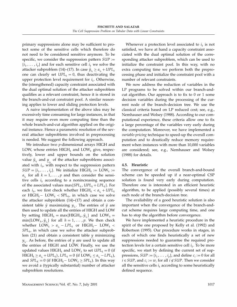
refer to the successfully solved instances only. Table 6

reports similar statistics for 8×6×4 tables of different

structures. In all cases, computing times are expressed

in wall-clock seconds of a PC Pentium II/400 with

64 Mbyte RAM.

Notice that random instances appear harder to

solve than the real-world ones, due to the lack of a

strong structure in the table entries. Nevertheless, we

could solve most of them to proven optimality within

short computing time. In addition, for all instances

the quality of the heuristic solutions (r-HEU) found

at the root node after a few seconds of computation

(r-time) is significantly better than the one found by

the initial heuristic (HEU1).

7. ConclusionsCell suppression is a widely used methodology in

Statistical Disclosure Control. In this paper we have

introduced a new integer linear programming model

for the cell suppression problem, in the very gen-

eral context of tables whose entries are subject to a

generic system of linear constraints. Our model then

covers k-dimensional tables with marginals as well as

hierarchical and linked tables. To our knowledge, this

is the first attempt to model and solve the cell sup-

pression problem in such a very general context. We

have also outlined a possible solution procedure in

the branch-and-cut framework. Computational results

on real-world instances have been reported. In par-

ticular, we were able to solve to proven optimality,

for the first time, real-world 4-dimensional tables with

marginals as well as linked tables. Extensive computa-

tional results on a test-bed containing 1,160 randomly-

generated 3- and 4- dimensional tables have been also

given.

AcknowledgmentWork partially supported by the European Union project IST-2000-

25069, Computational Aspects of Statistical Confidentiality (CASC),

coordinated by Anco Hundepool (Central Bureau of Statistics,

Voorburg, The Netherlands). The first author was supported by

M.U.R.S.T. (“Ministero della Ricerca Scientifica e Tecnologica”) and

by C.N.R. (“Consiglio Nazionale delle Ricerche”), Italy, while the

second author was supported by “Ministerio de Educación, Cultura

y Deporte,” Spain.

ReferencesApplegate, D., R. Bixby, W. Cook, V. Chvátal. 1995. Finding cuts

in the traveling salesman problem. DIMACS technical report

95-05, Center for Research on Parallel Computation, Rice Uni-

versity, Houston, TX.

Caprara, A., M. Fischetti. 1997. Branch-and-cut algorithms.

M. Dell’Amico, F. Maffioli, S. Martello, eds. Annotated Bibliogra-phies in Combinatorial Optimization. John Wiley & Sons.



Cox, L. H. 1980. Suppression methodology and statistical disclosure

control. J. Amer. Statist. Assoc. 75 377–385.. 1995. Network models for complementary cell suppression.

J. Amer. Statist. Assoc. 90 1453–1462.Crowder, H. P., E. L. Johnson, M. W. Padberg. 1983. Solving large-

scale zero-one linear programming problems. Oper. Res. 31803–834.

Carvalho, F. D., N. P. Dellaert, M. S. Osório. 1994. Statistical disclo-

sure in two-dimensional tables: General tables. J. Amer. Statist.Assoc. 89 1547–1557.

Dellaert, N. P., W. A. Luijten. 1996. Statistical disclosure in gen-

eral three-dimensional tables. Technical paper TI 96-114/9,

Tinbergen Institute, Rotterdam, The Netherlands.

Fischetti, M., J. J. Salazar. 1999. Models and algorithms for the

2-dimensional cell suppression problem in statistical disclosure

control. Math. Programming 84 283–312.Geurts, J., 1992. Heuristics for cell suppression in tables. Work-

ing paper, Netherlands Central Bureau of Statistics, Voorburg,

The Netherlands.

Gusfield, D., 1988. A graph theoretic approach to statistical data

security. SIAM J. Comput. 17 552–571.Kao, M. Y., 1996. Data security equals graph connectivity. SIAM J.

Discrete Math. 9 87–100.

Kelly, J. P., 1990. Confidentiality protection in two- and three-

dimensional tables. Ph.D. dissertation, University of Maryland,

College Park, MD.

Kelly, J. P., B. L. Golden, A. A. Assad. 1992. Cell suppression:

Disclosure protection for sensitive tabular data, Networks 22397–417.

Nemhauser, G. L., L. A. Wolsey. 1988. Integer and combinatorial opti-mization. John Wiley & Sons.

Padberg, M., G. Rinaldi. 1991. A branch-and-cut algotithm for the

resolution of large-scale symmetric traveling salesman prob-

lems. SIAM Rev. 33 60–100.Robertson, D. A. 1995. Cell suppression at Statistics Canada.

Proc. Second Internat. Conf. Statist. Confidentiality. Luxem-

bourg.

Sande, G. 1984. Automated cell suppression to preserve confiden-

tiality of business statistics. Statist. J. United Nations ECE 233–41.

. 1998. Blunders official statitical agencies make while pro-

tecting the confidentiality of business statistics. Internal report,

Sande and Associates.

Willenborg, L. C. R. J., T. de Waal. 1996. Statistical disclosure

control in practice. Lecture Notes in Statistics 111. Springer,

New York.

Accepted by Thomas M. Liebling; received October 1999. This paper has been with the authors 2 months for 1 revision.


Documents

Solving the Cell Suppression Problem on Tabular Data with Linear Constraints