arX

iv:h

ep-t

h/96

0510

5v1

15

May

199

6

LPTENS–95/25,hep-th/9605105,

May 1996.

SOLVING THE STRONGLY COUPLED 2D GRAVITY

III: STRING SUSCEPTIBILITY AND

TOPOLOGICAL N-POINT FUNCTIONS

Jean-Loup GERVAIS

Jean-Francois ROUSSEL

Laboratoire de Physique Theorique de l’Ecole Normale Superieure1,

24 rue Lhomond, 75231 Paris CEDEX 05, France.

Abstract

We spell out the derivation of novel features, put forward earlier in a letter, of twodimensional gravity in the strong coupling regime, at CL = 7, 13, 19. Within the oper-ator approach previously developed, they neatly follow from the appearence of a newcosmological term/marginal operator, different from the standard weak-coupling one,that determines the world sheet interaction. The corresponding string susceptibilityis obtained and found real contrary to the continuation of the KPZ formula. Stronglycoupled (topological like) models—only involving zero-mode degrees of freedom—aresolved up to sixth order, using the ward identities which follow from the dependenceupon the new cosmological constant. They are technically similar to the weakly cou-pled ones, which reproduce the matrix model results, but gravity and matter quantumnumbers are entangled differently.

1Unite Propre du Centre National de la Recherche Scientifique, associee a l’Ecole NormaleSuperieure et a l’Universite de Paris-Sud.

1 Introduction

The truncation of the chiral operator algebra at CL = 7, 13, 19 seems to be the keyto the strong coupling regime of two dimensional gravity2. After the first hints[2],the trucations theorems were proven at the level of primaries (for half integer spins)in ref.[3], the final complete proof being given in a recent paper of ours[4]. In ref.[5],and in the present article, we analyse further the physics of these theories and beginsolving the topological models proposed in ref.[4], where gravity is in the strongcoupling regime.

In the strong coupling regime, the screening charges are complex, so that thedimensions of primaries are not real in general. These truncation theorems expressthe fact that, nevertheless, at the special values of CL the operator algebra of thechiral intertwinors—that appear as chiral components of the powers of the Liou-ville exponentials—has a consistent restriction to Verma modules with real Virasorohighest weights. Thus one is led to consider that strongly coupled two dimensionalgravity should be expressible entirely in terms of the corresponding chiral compo-nents. This brings in drastic changes with respect to the weakly coupled regime.It rules out the Liouville exponentials, which are the well known local fields of thepresent description of 2D gravity in the conformal gauge, both classically and at theweakly coupled quantum level[3]. However, a new set of local fields may be con-structed, which is consistent with the truncation theorems. Then the correspondingphysics follows quite naturally, using methods very similar to the weak couplingones.

In ref.[4] we emphasized that the transition from weak to strong coupling may becharacterized by a deconfinement of chirality. Indeed, in the weak coupling regime,the Liouville exponentials may be consistently restricted to the sector where left andright chiral components have the same Virasoro weight, so that we may say that chi-rality (of gravity) is confined. In this regime, the quantum numbers associated witheach screening charge may take independent values. In the strong coupling regime,on the contrary, the reality condition forces us to link the quantum numbers associ-ated with the two screening charges, for each chirality. This is however incompatiblewith the equality between left and right weights, so that the (gravity) chirality fluc-tuates: it is deconfined. The main motivation to study the strongly coupled regimeis of course the building of the (so called) non critical strings. Indeed, the balance ofcentral charges prevents us from doing so in the weak coupling regime. The actualconstruction is still too complicated beyond the three point functions, but we haveset up[4, 5] models—which we call topological since their only degrees of freedomare zero modes—where gravity is strongly coupled. We shall present details abouttheir solution which were left out from ref.[5].

The article is organised as follows. In section 2 we derive the string susceptibility,drawing a parallel with the weak coupling calculation. In section 3, we study thethree point functions of our topological models. It was derived earlier[4] only withthe same screening choice for the three legs, but we need to treat the mixed case.Section 4 is devoted to the derivation of the N point function from the Ward identitiesgenerated by taking derivatives with respect to the strong-coupling cosmologicalconstant. Using Mathematica, we derive irreducible irreducible vertices, up to six

2Evidence that a similar mechanism is at work for W3 gravity are given in ref.[1].

1

legs, which give a consistent perturbation theory up to sixth order. This is similarto earlier studies in the weak coupling regime[10] but we let the screening numberfluctuate, contrary to this reference. Consistency of the perturbative expansion ofthe topological models leads us to counting rules for its relation with the Feynmanpath integrals, which could not be guessed a priori. However, at the end we verifythat the same rules also hold in the weak coupling regime, if the screening numbersare allowed to fluctate. As a matter of fact, the two types of topological models (i.e.the continuous version of matrix models, and our new ones) are found to be verysimilar technically, although gravity and matter quantum numbers are entangledcompletely differently.

2 The string susceptibility

2.1 The weak coupling case revisited

To begin with, we review the derivation in the weak coupling regime, followingessentially ref.[7]. We shall provide details left out previously which will shed lighton the strong coupling case. In particular, it will be useful to draw a close parallelwith the DDK argument. With our notations, the latter follows from the following3

effective action, with cosmological constant µc, background metric g:

S(w)µc

= − 1

8π

∫dzdz

√−g{gab∂aΦ∂bΦ + QLR(2)Φ + µce

α−Φ}, (2.1)

The two screening charges α± and QL are related as usual:

α−α+ = 2, α− + α+ = QL, (2.2)

and the Liouville central charge is such that

CL = 1 + 3Q2L. (2.3)

For CL > 25, α± are real; this is the weak coupling regime. For 25 > CL > 1, α± arecomplex; this is the strong coupling situation which we want to study further in thepresent article. The Virasoro weight of the operator exp(−βΦ) is ∆G = −1

2β(β+QL).

Recall the basic point of DDK. Consider the correlator

⟨∏

ℓ

e−βℓΦ(zℓ,zℓ)

⟩(νh)

µc

≡∫DφeS

(w)µc

(∏

ℓ

e−βℓφ(zℓ,zℓ)

)(νh)

, (2.4)

νh is the number of handles. The notation is that Φ is the Liouville operator, while φis the c-number field that appears in the functional integral. The latter is unchangedif we change variable by letting φ = φ − ln(µc)/α−. This gives

⟨∏

ℓ

e−βℓΦ(zℓ,zℓ)

⟩(νh)

µc

=

⟨∏

ℓ

e−βℓΦ(zℓ,zℓ)

⟩(νh)

1

µ[∑

ℓβℓ+QL(1−νh)]/α−

c . (2.5)

3 The upper index “(w)” is to recall that this effective action is relevent to the weak couplingregime.

2

the last term comes from the linear term of the action and the Gauss-Bonnet theorem

1

8π

∫ ∫dzdzR(2) = (1 − νh). (2.6)

Now, we compare this procedure with the corresponding discussion in the operatormethod. There, the operator algebra of each chiral component has a quantum groupsymmetry4 of the type Uq(sl(2)) ⊙ Uq(sl(2)), with

q = eih, q = eih, h = πα2−

2, h = π

α2+

2. (2.7)

The two quantum group parameters are related by

hh = π2, h + h =CL − 13

6. (2.8)

The first relation shows that they are, in a sense, dual pairs. The above symbol⊙ has a special meaning which was much discussed before[11, 4, 8]. The Hilbertspace of states is of course a direct sum of products of a left and a right VirasoroVerma modules. These are characterized by the eigenvalue of the rescaled zero-mode momenta , of the Backlund free field with chiral components ϑR(x),ϑL(x) defined by writing on the cylinder,

ϑR(x) = q0 + ip0x + i∑

n 6=0

e−inx pn

n, =

2i

α−

p0,

ϑL(x) = q0 + ip0x + i∑

n 6=0

e−inxpn

n, =

2i

α−

p0. (2.9)

A right Verma module is charaterized by the highest-weight eigenvalue

∆() =h

4π(2

0 − 2), 0 = 1 +π

h(2.10)

of L0, with similar formulae for the left Verma modules. For = ±0, ∆ van-ishes. This describes the two Sl(2, C) invariant states. In ref.[7], it was shown thatthe transformation law Eq.2.5 corresponds to the following definition for arbitrarycosmological constant:

e−βΦ(µc)

= µβ/α−

c µ−/2c e−βΦ µ/2

c . (2.11)

From this it is easy to recover the standard results for νh = 0, and 1. First, considerthe sphere (νh = 0). In the operator method, the left hand side of Eq.2.5 is givenby ⟨

∏

ℓ

e−βℓΦ(zℓ,zℓ)

⟩(0)

µc

=< −0,−0|∏

ℓ

e−βℓΦ(µc)

|0, 0 > . (2.12)

where the notation |0, 0 > represents the state with left and right weights ∆ =∆ = 0. Making use of Eq.2.11, we get

⟨∏

ℓ

e−βℓΦ(zℓ,zℓ)

⟩(0)

µc

= µ∑

ℓβℓ

c < −0,−0|µ−/2c

∏

ℓ

e−βℓΦµ/2c |0, 0 > .

4 For recent developments in this connection see refs.[8],[9].

3

The contribution of the term QLR(2)Φ of the effective action is recovered whenµ±/2

c hit the left and right vacuua, since, according to Eq.2.2, QL/α− = 0, andthe result follows for νh = 0. Next, for the torus νh = 1, one should take the tracein the Hilbert space:

⟨∏

ℓ

e−βℓΦ(zℓ,zℓ)

⟩(1)

µc

= Tr

[∏

ℓ

e−βℓΦ(µc)

]. (2.13)

Making again use of Eq.2.11, we now get

⟨∏

ℓ

e−βℓΦ(zℓ,zℓ)

⟩(0)

µc

= µ∑

ℓβℓ

c Tr

[µ−/2

c

∏

ℓ

e−βℓΦµ/2c

]= µ

∑ℓβℓ

c

⟨∏

ℓ

e−βℓΦ(zℓ,zℓ)

⟩(0)

1

Thus, we get the same result without the term QL/α−. This agrees with Eq.2.5with νh = 1.

In order to compute the string susceptibilty, we next consider

Z(νh)(µc)

(A) ≡⟨δ[∫

dzdzeα−Φ − A]⟩(νh)

µc

. (2.14)

It is clear, from the form of the µc dependence of exp(−βΦ) that, without enteringinto the detailed definition of the δ function, we should have

δ[∫

dzdzeα−Φ − A]

µc

= µ−/2c δ

[∫dzdzµ−1

c eα−Φ − A]

1µ/2

c . (2.15)

Consider the sphere, one gets

Z(0)(µc)

(A) =< −0,−0|µ−/2c δ

[∫dzdzµ−1

c eα−Φ − A]

1µ/2

c |0, 0 > .

Z(0)(µc)

(A) = µ1+Q/α−

c Z(0)(1) (Aµc).

Assuming that for large area Z(0)(µc)

(A) ∼ Aγstr−3, this gives the well known result

γstr = 2 − Q/α− = 1 − π

h. (2.16)

A similar discussion also gives back the standard result for νh = 1.Next we describe the cosmological dependence of the chiral components which is

such that Eq.2.11 holds. Our basic assumption will be that it remains the same forthe strong coupling regime. Contact with the quantum group classification is madeby letting

β = α−J + α+J . (2.17)

Then the corresponding local Liouville exponential operator is given by[3, 6]

e−βΦ(z, z) =∑

m, m

V(J, J)

m m(z) V

(J, J)

m m (z) (2.18)

This form is dictated by locality and closure under fusion. The notation for thechiral operators refers to a particular normalization whose precise expression will

4

be needed later on. In ref.[5], it was remarked that Eq.2.11 is derivable from thefollowing generalised Weyl transformation law

V(J J)

m m (µ)= µJ+Jπ/hµ−/2V

(J J)

m mµ/2

V(J J)

m m (µ) = µJ+Jπ/hµ−/2V(J J)

m m µ/2. (2.19)

Taking two different parameters µ and µ is only relevent for the strong couplingcase. For the weak coupling one, the left and right quantum numbers are all equal(chirality is confined) so that in deriving Eq.2.11, one only deals with the productµµ. The previous discussion is immediately recovered with µc = µµ.

2.2 The strong coupling regime

At this point we turn to the strong coupling regime. Now 1 < CL < 25. Thescreening charges α± are complex and related by complex conjugation. Thus com-

plex weights appear in general. The weight of a chiral operator V(J J)

m mis equal to

∆(J,J

), with J,J

= 0 + 2J + 2Jπ/h. We shall denote by |J, J > the corre-sponding highest weight state. There are two types of exceptional cases such thatthe weights are real. These are the states |J, J > (resp. | − J − 1, J >), withnegative (resp. positive) weights. One could try to work with the correspondingLiouville exponentials exp[−J(α− − α+)Φ] (resp exp[((J + 1)α− − α+)Φ]), but thiswould be inconsistent, since these operators do not form a closed set under fusingand braiding. Moreover,the chiral vertex operators are such that

< J2, J2|V (JJ)

mm|J1, J1 >∝ δJ1, J2−m δ

J1, J2−m. (2.20)

As a result, it follows from Eqs.2.18, that Liouville exponential operators do notpreserve the reality condition for highest weights just recalled. The basic problem isthat Eq.2.18 involves the V operators with arbitrary m m, while the reality conditionforces us to only use V operators of the type

V(J)m, + ≡ V

(−J−1,J)−m m , or V

(J)m,− ≡ V (J,J)

m m . (2.21)

Next recall that the truncation theorems hold for

C = 1 + 6(s + 2), s = 0,±1. (2.22)

For these values, there exists a closed chiral operator algebra restricted to the phys-ical Hilbert space

H±phys ≡

1∓s⊕

r=0

∞⊕

n=−∞

H±r/2(2∓s)+n/2 (2.23)

where H±J denotes the Verma modules with highest weights |∓ (J +1/2)−1/2, J >.

The physical operators χ(J)± are defined for arbitrary5 2J ∈ Z/(2 ∓ s), and 2J1 ∈

Z/(2 ∓ s). to be such that6

χ(J)± PH±

J1

=∑

ν≡J+m∈Z+

(−1)(2∓s)(2J1+ν(ν+1)/2)V(J)m,± PH±

J1

, (2.24)

5 By the symbol Z/(2± s), we mean the set of numbers r/(2± s) + n, with r = 0, · · ·, 1± s, ninteger; Z denotes the set of all positive or negative integers, including zero.

6Z+ denotes the set of non negative integers.

5

where PH±

J1

is the projector on H±J1

. According to the formulae previously recalled,

their weights are, respectively,

∆−(J, CL) = −CL − 1

6J(J + 1), ∆+(J, CL) = 1 +

25 − CL

6J(J + 1). (2.25)

Note that the cases of positive and negative weights are completely separated opera-torially, eventhough we discuss them simultaneously to avoid repetitions. Moreover,the definition of V

(J)m, + is not symmetric between the two screening charges. For the

left components, it is appropriate to make the other choice7

V(J)m,+ ≡ V

(J,−J−1)

−m m , V(J)m,− ≡ V

(J,J)

m m . (2.26)

With this, one defines the left physical fields by a formula similar to Eq.2.24:

χ(J)± P

H±

J1

=∑

ν≡J+m∈Z+

(−1)(2∓s)(2J1+ν(ν+1)/2)V(J)m,± P

H±

J1

, (2.27)

Since Eqs.2.25 are invariant under J → −J − 1, we get the same formuale for theweights of the left physical operators just defined:

∆−(J, CL) = −CL − 1

6J(J + 1), ∆

+(J, CL) = 1 +

25 − CL

6J(J + 1), (2.28)

The particular way to define the left and right components just summarised has an-other motivation, which we stressed already before. Complex conjugation exchanges

the two screening charges, so that the operators χ(J)+ , and χ

(J)+ are not hermitian.

The present choice ensures that the amplitudes are nevertheless invariant undercomplex conjugation if we exchange left and right quantum numbers.

Now we have enough recollection to turn back to the string susceptibility. Asis well known, the basic tool of the weak coupling derivation, was the existence ofthe cosmological term exp(α−Φ), of weight (1, 1), whose integral over z z definesthe invariant area and may be added to the free field action (see Eq.2.1) withoutbreaking conformal invariance. In the strong coupling regime, this cosmologicalterm is not acceptable since it does not preserve the reality conditions. On theother hand, Eqs.2.25 2.28 are clearly such that ∆+(0, CL) = ∆

+(0, CL) = 1. As we

pointed out earlier, the corresponding operator

V0,0 = χ(0)+ (z)χ

(0)+ (z). (2.29)

defines a new cosmological term and is local. Thus the area element of the strongcoupling regime is χ

(0)+ (z)χ

(0)+ (z)dzdz. It is factorized into a simple product of a

single z component by a z component. The effective action Eq.2.1 should be mod-ified accordingly. However, it is reasonable to assume that the behaviour underglobal rescaling (global Weyl transformation) of the chiral components will remainessentially the same. Moreover, the reality condition recalled above led us[5] to takeµ = µh/π, with µ real. According to Eq.2.19, this gives

χ(J)+ (µ) = µ−J−1+Jπ/hµ−/2χ

(J)+ µ/2

χ(J)+ (µ) = µJh/π−(J+1)µ−h/2πχ

(J)+ µh/2π. (2.30)

7 This is actually a notational convenience, since clearly the two choices are exchanged by lettingJ → −J − 1

6

For the cosmological term this gives

V0,0(µc)

= µ−1c µ−(+h/π)/4

c V0,0(1) µ(+h/π)/4

c , (2.31)

where we have let µc = µ2, so that the overall factor becomes µ−1c as it should. From

there, the computation of the string susceptibility, already summarised in ref.[5] goesas follows. Consider, now the expectations values similar to Eq.2.14

Z(νh)µc

(A) ≡⟨δ[∫

dzdzχ(0)+ (µc)

χ(0)+ (µc)

− A]⟩(νh)

µc

. (2.32)

At this time, we only have the operator method at our disposal, so that we maydefine the right hand side only for νh = 0, and νh = 1 as, respectively,

Z(0)µc

(A) ≡ < −0, −0|δ[∫

dzdzV0,0 − A]

(µc)|0, 0 >,

Z(1)µc

(A) ≡ Tr

{δ[∫

dzdzV0,0 − A]

(µc)

}. (2.33)

Again we shall not need the detailed definition of the delta function. Only the Weyltramsformation, analogous to Eq2.15 will matter, that is

δ[∫

dzdzV0,0 − A]

(µc)= µ−(+h/π)/4

c δ[∫

dzdzµ−1c V0,0 − A

]

(1)µ(+h/π)/4

c .

(2.34)From there on the calculation proceeds exactly as in the weak coupling regime, andwe shall not repeat it . The basic point is that the factors µ±(+h/π)/4

c give realeigenvalues when they hit the left or right vacua, since 0(1 + h/π) = (CL − 1)/6.This is contrast with the weak coupling factors µ±/2

c that would give complex resulthere. It came out from our choice of µ, µ, which therefore ensures the reality of thestring susceptibility. For νh = 0 one finds γstr = (2 − s)/2. Comments about thisresult were given in ref.[5].

3 The three-point functions

3.1 The gravity coupling constants revisited

The Verma modules of gravity are conveniently characterized by the eigenvalue ofthe rescaled momentum . The spectrum of eigenvalue is of the form

J, J=

0 + 2J + 2Jπ/h. The starting point to derive the three-point functions is theexpression[4] of the matrix element of the V fields recalled above between suchhighest weight states. It is convenient to rewrite it under the form

< −3|V (J1J1)

mm|2 >= δJ2−J3−m,0 δ

J2−J3−m,0g−3

1,2

g−31,2

= (−1)νν(i/2)ν+ν Hνν(1)Hνν(2)Hνν(3)

Hνν(ν/2,ν/2)(3.1)

with

i = 0 + 2Ji + 2π

hJi, i = 1, 2, 3;

ν + νπ

h=

1

2(1 + 2 + 3 − 0) ≡ νe (3.2)

7

The g’s are called coupling constants. Each factor Hνν() was shown to be ex-pressible as a sum over path. It is convenient to write it under the form (with = 0 + 2J + 2J π

h)

Hνν() =(−π

h

)−(1/4+J)ν(−h

π

)−(1/4+J)ν ~www

− νe

~www. (3.3)

In general we define the symbol~wwBe

Ae

~ww for Be − Ae ≡ νe = ν + ν πh, with ν and ν

positive integers, as the following product of factors along a general path

~wwwBe

Ae

~www =N−1∏

ℓ=0

(−π

h

)Rℓ−1/2

F

[Re

ℓ + Reℓ+1

2− h

2π

]

ǫℓ/2

×

N−1∏

ℓ=0

(−h

π

)Rℓ−1/2

F

[Re

ℓ + Reℓ+1

2− π

2h

]

ǫℓ/2

, (3.4)

where the product is taken along any path going from Ae to Be with intermediatepoints Re

ℓ , such that

Reℓ+1 − Re

ℓ = ǫℓ +π

hǫℓ, ǫℓ = 0, ±1, ǫℓ = 0, ±1, ǫℓǫℓ = 0;

Re0 = Ae, Re

N = Be, Reℓ = Re

ℓ

h

π, Re

ℓ = Rℓ +π

hRℓ. (3.5)

Note that we shall always be in the case where Rℓ and Rℓ are rational, while hπ

is not. Thus the last equation is unambiguous. We shall not bother about theprecise choice of sheet for square root of gamma functions. It should be specifiedaccording to ref.[7]. It is not important since it will only appear in the final legfactors. This product does not depend upon the choice of path8. Up to the factorwe have put in front of Eq.3.3 it coincides with the one introduced in refs.[4], [11].One may visualise the path as made up with N segments of coordinates ǫℓ, ǫℓ,starting from the point specified by Re

ℓ . Using the fact that ǫℓǫℓ = 0, one may

rewrite the factors (−π/h)Rℓ−1/2, and (−h/π)Rℓ−1/2 may be rewritten, respectively

as (−π/h)(Rℓ+Rℓ+1−1)/2, and (−h/π)(Rℓ+Rℓ+1−1)/2, so that our definition only involvesthe midpoints (Re

ℓ + Reℓ+1)/2 of each segment. It is easy to verify that we have the

composition law ~wwwBe

Ae

~www

~wwwCe

Be

~www =

~wwwCe

Ae

~www (3.6)

So far, we assumed that ν and ν are positive integers. This last relation allows us toextend the definition to arbitrary signs. Next, it is useful to use the fact that F (z)satisfies the relation F (1 − z) = (F (z))−1 to derive the identity

~wwwBe

Ae

~www =

~wwww1 + π

h− Be

1 + πh− Ae

~wwww. (3.7)

8 This may be seen, in particular, by making use of ref.[12]

8

Returning to Eq.3.1, one finds that it may be written as

g−31,2

= (−1)νν(

i

2

)ν+ν (−π

h

)(ν−ν)/2 ~www1

1 − νe

~www~www

2

2 − νe

~www~www

3

3 − νe

~www~www

0

−νe

~www.

(3.8)The last term has been retransformed using Eq.3.7 so that it takes the same formas the other three with = 0. Letting 4 = 0, we may thus write compactly

g−31,2

= (−1)νν(

i

2

)ν+ν (−π

h

)(ν−ν)/2 4∏

i=1

~wwwi

i − νe

~www (3.9)

3.2 The dressings

3.2.1 The weak coupling case

In the weak coupling regime, one represents[7] matter by another copy of the Li-ouville theory with a different central charge. Following our previous works thesymbols pertaining to matter are noted with a prime (or, if convenient, with anindex M). The relations between matter and gravity parameters are

CM = 26 − CL, h/π = −π/h′, α′± = ∓iα∓. (3.10)

One constructs local fields in analogy with Eq.2.18:

e−(J ′α′− + J ′α′

+)Φ′(z, z) =∑

m, m

V ′ (J ′, J ′)

m m(z) V

′ (J ′, J ′)

m m(z). (3.11)

Φ′(z, z) is the matter field (it commutes with Φ(z, z)), There are two possible dress-ing of these operators by gravity such that the total weights are ∆ = ∆ = 1. Thefirst is achieved by considering the vertex operators

WJ ′,J ′ ≡ e−((−J ′ − 1)α− + J ′α+)Φ − (J ′α′− + J ′α′

+)Φ′

(3.12)

In particular for J ′ = J ′ = 0, we get the cosmological term exp(α−Φ). For theassociated Liouville zero modes, this means that

J,J= −′

J ′,J ′. The other choice

of dressing leads to the operators

WJ ′,J ′

conj = e−(J ′α− − (J ′ + 1)α+)Φ − (J ′α′− + J ′α′

+)Φ′

. (3.13)

3.2.2 The strong coupling case

We consider another copy of the strongly coupled theory, with central charge CM =26 − CL. Since this gives CM = 1 + 6(−s + 2), we are also at the special values,and the truncation theorems applies to matter as well. This “string theory” has notransverse degree of freedom, and is thus topological. The complete dressed vertexoperator are now

VJ ′,J′

= χ(J ′)+ χ

(J′)

+ χ′ (J ′)− χ′ (J

′)

− , (3.14)

VJ ′,J′

conj = χ(−J ′−1)+ χ

(−J′−1)

+ χ′ J ′)− χ′ J

′

− . (3.15)

As in the weak coupling formula, operators relative to matter are distinguished bya prime. The gravity part is taken to have positive weights so that it includes thecosmological term.

9

3.3 The matter coupling constants revisited

It is convenient to define symbols~wwB′e

A′e

~ww′related to matter, similar to

~wwBe

Ae

~ww. Let

~wwwwB′e

A′e

~wwww

′

=N−1∏

ℓ=0

(π

h′

)R′ℓ−1/2

F

[R′e

ℓ + R′eℓ+1

2− h′

2π

]

ǫ′ℓ/2

×

N−1∏

ℓ=0

(h′

π

)R′ℓ−1/2

F

[R′e

ℓ + R′eℓ+1

2− π

2h′

]

ǫ′ℓ/2

. (3.16)

It is the direct analogue of Eq.3.5, apart from a simple modification, namely,

we put the factors (π/h′)R′ℓ−1/2, and (h′/π)R′

ℓ−1/2, instead of (−π/h′)R′

ℓ−1/2, and

(−h′/π)R′ℓ−1/2. As we alradry know[7, 4, 5], tremendous simplifications occur when

gravity and matter are put together. Our definitions are such that this appearsneatly the level of the product symbols. Indeed, let us derive the following basicrelations ~wwww

B′e

A′e

~wwww

′

=

~wwww1 + π

hA′e

1 + πhB′e

~wwww =

~wwww

πh(1 − A′e)

πh(1 − B′e)

~wwww. (3.17)

The equality between the last two expressions is a direct consequence of Eq.3.7. Inorder to derive the first equality, one transforms the first line of Eq.3.16 by writing

F

[R′e

ℓ + R′eℓ+1

2− h′

2π

]=

{F

[1 − R′e

ℓ + R′eℓ+1

2− π

2h

]}−1

Let us define the associated path in Liouville theory by Reℓ = 1 − R′e

ℓ, so that the

second term becomes the inverse of the Liouville factor F[

Reℓ+Re

ℓ+1

2− π

2h

]. On the

other hand, an easy calculation shows that for the other F we have

F

[R′e

ℓ + R′eℓ+1

2− π

2h′

]= F

[Re

ℓ + Reℓ+1

2− h

2π

].

It follows from the relations given above that Rℓ = 1− R′ℓ, and Rℓ = R′

ℓ. Thereforethe associated path of gravity is such that ǫℓ = ǫ′ℓ, ǫℓ = −ǫ′ℓ. This allows to verifythat all the other factors also match, and Eq.3.17 follows.

Finally, the matter coupling is given by

g′−′3

′1,′

2=(

i

2

)ν′+ν′ (π

h′

)(ν′−ν′)/2 4∏

i=1

~wwww′

i

′i − ν ′e

~wwww

′

(3.18)

3.4 The leg factors

In this part, we rediscuss the simplifications that occur when gravity and matterare put together at the most basic level, that is, when the coupling constants aremultiplied. As originally discussed in [7], and as we just saw, the dressing conditionshave a simple expression in terms of the ’s, namely, one must have ′ = ±. Thetwo choices of sign corresponds to the two possible screening charges, and are treatedmuch in the same way. There are in fact only two really different situations, the firstwhen one takes the same dressing condition on all three legs—this is the case wehave considered in our previous works—and the second when one of the screeningcharges is of the opposite type. Let us discuss them in turn.

10

3.4.1 The same choice for every legs

This situation was discussed at length before. We return to it briefly as a preparationfor the mixed screening choice. First consider the case where ′

i = i ≡ hπi. Note

that, since by definition 4 = 0, the same screening condition holds (trivially) fori = 4. Applying the formulae given above one finds that νe′ = h

π(νe + 1), and

~wwww′

i

′i − νe′

~wwww

′

=~www

i − νe

i + 1

~www.

Making use of Eq.3.6 this leads to

~wwww′

i

′i − νe′

~wwww

′~wwwi,

i − νe

~www =

~wwwi

i + 1

~www =

(−π

h

)2Ji+1/2

F [i]

−1/2

.

Altogether, we get a product of leg factors

g−312

g′− 3

1 2= (−1)νν

(i

2

)2ν−1(−h

π

)2ν 4∏

i=1

1√

F [i]. (3.19)

The other screening condition ′i = −h

πi is treated similarly, obtaining

g−312

g′ 3

− 1− 2= (−1)νν

(i

2

)2ν−1 (−π

h

)2ν 4∏

i=1

1√

F [i]. (3.20)

3.4.2 The mixed case

The coupling constant g−312

is completely symmetric and, by relabelling, we mayalways choose the third leg to be the one which differs from the others. Again thereare two cases. First choose ′

i = hπi for i = 1, 2, and ′

3 = −hπ3. The relation

between νe and νe′ may be written as νe′ = hπ(νe − 3 + 1). A simple modification

of a calculation performed above then gives, for i = 1, 2,

~wwww′

i

′i − νe′

~wwww

′~wwwi

i − νe

~www =

~wwwi − νe + 3

i + 1

~www

~wwwi

i − νe

~www

=

~wwwi

i + 1

~www

~wwwi − νe + 3

i − νe

~www (3.21)

where we have used the multiplication law Eq.3.6. For i = 3, we write insteadνe′ = −h

πνe − 1 + h

π(1 + 2). One now gets

~wwww′

3 − νe′

′3

~wwww

′~www3 − νe

3

~www =

~wwww3

3 + πh

~wwww

~www3 − νe + 1 + 2.

3 − νe

~www (3.22)

The last term in Eq.3.8 may be treated in the same way as the third, and the resultis given by the last equation with 3 → 0. Altogether, one gets

g−312

g′ 3

1 2=(

i

2

)2(J3−J1−J2)+1 (−π

h

)ν−ν (−1)νν

√F [0]

1√

F [1]

1√

F [2]

1√

F [3]. (3.23)

11

When one performes the computation, one first arrives at the right hand side mul-tiplied by the factor

~www1 + 3 − νe

1 − νe

~www~www

2 + 3 − νe

2 − νe

~www~www

1 + 2 + 3 − νe

3 − νe

~www~www

1 + 2 − νe

−νe

~www.

Making use of Eq.3.17, one may verify that it is equal to one, thereby completingthe derivation. Thus in this case also the result is a product of leg factors. A similarcalculation allows us to deal with the other choice, obtaining

g−312

g′− 3

− 1− 2=(

i

2

)2(J3−J1−J2)+1(−h

π

)ν−ν(−1)νν

√F [0]

1√

F [1]

1√

F [2]

1√

F [3].

(3.24)

3.5 The three point functions.

The computation makes use of the relations just derived for the coupling constants.Let us first consider the weak coupling case for comparison. One gets with the

same screening on every legs9 :⟨∏

ℓ

WJ ′ℓ,J ′

ℓ

⟩=(g ′

3

− ′1− ′

2g′−′

3

′1′

2

)2

=1

F [0]

3∏

i=1

1

F [′i]

(3.25)

⟨3∏

ℓ=1

WJ ′ℓ,J ′

ℓ

conj

⟩=(g− ′

3

′1 ′

2g′−′

3

′1′

2

)2

=1

F [0]

3∏

i=1

1

F [′i]. (3.26)

In the weak coupling regime with one different screening, one gets⟨WJ ′

3,J ′3

conj

2∏

ℓ=1

WJ ′ℓ,J ′

ℓ

⟩=(g− ′

3

− ′1− ′

2g′−′

3

′1′

2

)2

=1

F [0]

1

F [′3]

2∏

i=1

1

F [′ℓ]

. (3.27)

Next consider the strong coupling case. First, in order to make contact with ourprevious work[4] let us consider the completely symmetric case

⟨∏

ℓ

VJ ′ℓ,J

′

ℓ

⟩= g

′3

− ′1− ′

2g′−′

3

′1′

2g− ′

3

′

1 ′

2

g′−′3

′1′

2=

1

F [0]

3∏

i=1

1√

F [′i]F [

′

i]. (3.28)

Next we shall rather make use of the non symmetric three-point function⟨VJ ′

3,J′

3

conj

2∏

ℓ=1

VJ ′ℓ,J

′

ℓ

⟩= g

− ′3

− ′1− ′

2g′−′

3

′1′

2g ′

3

′

1 ′

2

g′−′3

′1′

2=

1

F [0]

1√

F [′3]F [′

3]

2∏

i=1

1√

F [′i]F [

′

i]. (3.29)

All the expressions of coupling constants we have obtained involve a factor 1/F (0)which is divergent. We drop it from now on, since it may be reabsorbed by an overallchange of the normalization of the three point functions which will not matter forthe forthcoming discussion.

9up to separate multiplicative factors on each leg which we drop. See refs.[7], [11] for detailedcomputations of these factors, in some cases.

12

4 N-point functions

4.1 Strong coupling regime

As shown in ref.[10], and as we will recall below, the key tools in deriving the higherpoint functions of the weak coupling regime are the Ward identities which may bederived from the path integral formulation Eq.2.4, by taking derivatives with respectto the cosmological constant µc. In so doing, the details of the effective action arenot important. One only uses the fact that the dependence upon this parameter inEq.2.4 is entirely contained—by definition—in the last term of S(w)

µc. In the strong

coupling regime another cosmological term (V0,0) appears, and it is reasonable toassume that the higher point functions will be determined from the associated wardidentities. In this case, however, the vertex operators create and destroy gravitychirality, so that the effective action cannot be constructed out of an ordinary worldsheet boson. It should rather involve two independent chiral bosons with oppositechiralities. We leave its derivation for further studies, since its explicit form doesnot matter so much at present. We only assume that this theory can be describedby an effective action including the new cosmological term:

Sµc= S0 + µc

∫V0,0 (4.1)

where the action S0 does not depend on the cosmological constant µc. So, weconsider N-point correlators

∫e−SµcV−J1−1,−J1−1

conj VJ2,J2 ...VJN ,JN =⟨V−J1−1,−J1−1

conj VJ2,J2 ...VJN ,JN

⟩

µc

(4.2)

where the integral sign stands for the functional integration and the integration overthe position of the N insertion points. For notational simplicity we drop the primesof the spins appearing in the vertex operators. As before, making use of Eq.2.30 onederives the scaling law of these correlators:⟨V−J1−1,−J1−1

conj ...VJN ,JN

⟩

µc

=⟨V−J1−1,−J1−1

conj ...VJN ,JN

⟩

1µ

∑N

i=1Pi−(N

2−1)( s+2

2 )c (4.3)

with

Pi = P (Ji, J i) =QM

4[α′

−(Ji +1

2) + α′

+(J i +1

2)]. (4.4)

Derivation with respect to the cosmological constant of these N point functions givesN + 1 point functions with one external momentum put to zero:

∂

∂µc

⟨V−J1−1,−J1−1

conj VJ2,J2 ...VJN ,JN

⟩

µc

=⟨V−J1−1,−J1−1

conj VJ2,J2...VJN ,JNV0,0⟩

µc

. (4.5)

If this model can indeed be described by such an effective action, its perturbativeexpansion must yield Feynman rules. We already computed the three point verticespreviously and we represent it graphically with an outgoing momentum for the leg(J1, J1):

⟨V−J1−1,−J1−1

conj VJ2,J2VJ3,J3

⟩

µc

= Lconj

J1,J1LJ2,J2

LJ3,J3µ

P1+P2+P3−s+24

c =

J ,J3 3J ,J2 2

J ,J1 1

(4.6)

13

with

LJ,J =1

√F[(1 − h

π)(1 + 2J)

]F ([(1 − π

h)(1 + 2J)

]), (4.7)

Lconj

J,J=

1√

F[−(1 − π

h)(1 + 2J)

]F ([−(1 − h

π)(1 + 2J)

]), (4.8)

from previous sections. The particular three-point function⟨V−Ji−1,−Ji−1

conj V0,0VJi,Ji

⟩

µc

= µ2Pi−1c Lconj

Ji,JiL0,0LJi,Ji

(4.9)

is the derivative of the two point function. This allows us to compute it by takingthe primitive and get

⟨V−Ji−1,−Ji−1

conj VJi,Ji

⟩

µc

=1

2Pi

µ2Pic Lconj

Ji,JiLJi,Ji

(4.10)

by using that L0,0 = 1, which can be checked for every special value10 CL = 7, 13, 19.For amplitudes with truncated external legs, such a two point function is the inverseof the propagator, and its value is consequently given by11

Pµc(Ji, J i) = Pi

µ−2Pic

(Lconj

Ji,JiLJi,Ji

)=

J ,Ji i

. (4.11)

On the other hand, by taking derivatives, one gets higher order correlators. Thederivatives of the three point functions yields four point functions with one externalmoment put to zero. However, the N -point functions should be symmetric in theirN legs when expressed in terms of the variables we are using. (this is true for N = 3)and we get by symmetrisation the generic four-point function⟨V−J1−1,−J1−1

conj VJ2,J2VJ3,J3VJ4,J4

⟩

µc

= Lconj

J1,J1LJ2,J2

LJ3,J3LJ4,J4

µP1+P2+P3+P4−

s+22

c

(QM

4

[α′−(J1 + J2 + J3 + J4 + 1) + α′

+(J1 + J2 + J3 + J4 + 1)]− 1

)(4.12)

If we believe in this effective action description, it must yield Feynman rules byperturbative expansion. This total four point function 4.12 can therefore be obtainedfrom the following diagrams

= +++

(4.13)

the last one being the one particule irreducible amplitude. It is clear on this examplethat, by choosing one incoming and N − 1 outgoing momenta, we have consistently

10This property is again very specific to these central charges.11We rescaled by an unexplained factor (1/2) which will turn out necessary so that the Feynman

rules match with the derivation ones.

14

restricted ourselves to Feynman rules which only involve one particle irreduciblevertices of the same type. Our purpose here is to get those one particule irreduciblevertices, which are the basic ingredients of the theory. To do this, we shall substractfrom the total four point function 4.12 the first three diagrams of 4.13 which we shallcompute from the previous Feynman rules (the propagator 4.11 and the vertices 4.6with their selection rules12).

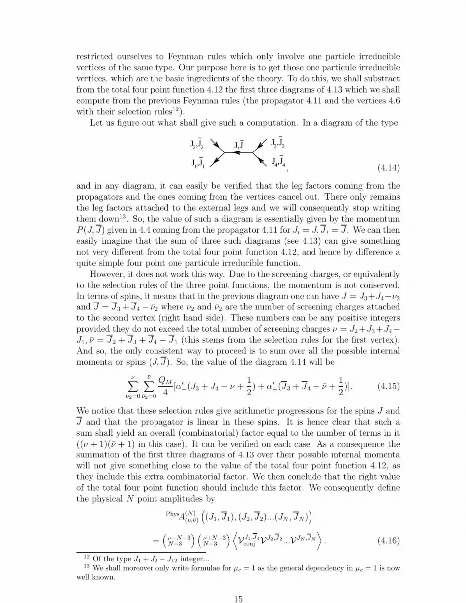
Let us figure out what shall give such a computation. In a diagram of the type

J ,J3 3J ,J2 2

J ,J1 1J ,J4 4

J,J

, (4.14)

and in any diagram, it can easily be verified that the leg factors coming from thepropagators and the ones coming from the vertices cancel out. There only remainsthe leg factors attached to the external legs and we will consequently stop writingthem down13. So, the value of such a diagram is essentially given by the momentumP (J, J) given in 4.4 coming from the propagator 4.11 for Ji = J, J i = J . We can theneasily imagine that the sum of three such diagrams (see 4.13) can give somethingnot very different from the total four point function 4.12, and hence by difference aquite simple four point one particule irreducible function.

However, it does not work this way. Due to the screening charges, or equivalentlyto the selection rules of the three point functions, the momentum is not conserved.In terms of spins, it means that in the previous diagram one can have J = J3+J4−ν2

and J = J3 + J4 − ν2 where ν2 and ν2 are the number of screening charges attachedto the second vertex (right hand side). These numbers can be any positive integersprovided they do not exceed the total number of screening charges ν = J2+J3+J4−J1, ν = J2 + J3 + J4 − J1 (this stems from the selection rules for the first vertex).And so, the only consistent way to proceed is to sum over all the possible internalmomenta or spins (J, J). So, the value of the diagram 4.14 will be

ν∑

ν2=0

ν∑

ν2=0

QM

4[α′

−(J3 + J4 − ν +1

2) + α′

+(J3 + J4 − ν +1

2)]. (4.15)

We notice that these selection rules give arithmetic progressions for the spins J andJ and that the propagator is linear in these spins. It is hence clear that such asum shall yield an overall (combinatorial) factor equal to the number of terms in it((ν + 1)(ν + 1) in this case). It can be verified on each case. As a consequence thesummation of the first three diagrams of 4.13 over their possible internal momentawill not give something close to the value of the total four point function 4.12, asthey include this extra combinatorial factor. We then conclude that the right valueof the total four point function should include this factor. We consequently definethe physical N point amplitudes by

PhysA(N)(ν,ν)

((J1, J1), (J2, J2)...(JN , JN)

)

=(

ν+N−3N−3

) (ν+N−3N−3

)⟨VJ1,J1

conj VJ2,J2...VJN ,JN

⟩. (4.16)

12 Of the type J1 + J2 − J12 integer...13 We shall moreover only write formulae for µc = 1 as the general dependency in µc = 1 is now

well known.

15

The combinatorial factors of the type(

ν+N−3N−3

)are the number of ways of placing ν

screening charges on the N − 2 vertices of a N point function14.Of course, this modifies the derivation rule 4.5 in the following way:

PhysA(N+1)(ν,ν)

((J1, J1), (J2, J2)...(JN , JN), (0, 0)

)

=(

ν + N − 2

N − 2

)(ν + N − 2

N − 2

)∂

∂µc

PhysA(N)(ν,ν)

((J1, J1), (J2, J2)...(JN , JN )

), (4.17)

which gives now for the four point function15

J ,J2 2

J ,J1 1 J ,J4 4

J ,J3 3

= PhysA(4)(ν,ν)

((J1, J1), (J2, J2), (J3, J3), (J4, J4)

)= (ν + 1)(ν + 1)×

(1 +

QM

4

[α′−(J1 + J2 + J3 + J4 + 1) + α′

+(J1 + J2 + J3 + J4 + 1)])

(4.18)

which differs from 4.12 by the simple factor (ν + 1)(ν + 1).Substracting from this total four point function the first three reducible diagrams

of 4.13, which are given by sums of the type 4.15, one gets the one particle irreduciblecorrelator

J ,J2 2

J ,J1 1 J ,J4 4

J ,J3 3

= 1PIA(4)(ν,ν)

((J1, J1), (J2, J2), (J3, J3), (J4, J4)

)

= (ν + 1)(ν + 1)1

4

(−(2 + s) +

QM

2(α′

−ν + α′+ν)

)(4.19)

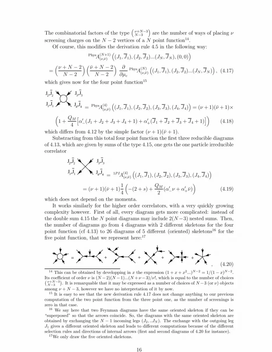
which does not depend on the momenta.It works similarly for the higher order correlators, with a very quickly growing

complexity however. First of all, every diagram gets more complicated: instead ofthe double sum 4.15 the N point diagrams may include 2(N−3) nested sums. Then,the number of diagrams go from 4 diagrams with 2 different skeletons for the fourpoint function (cf 4.13) to 26 diagrams of 5 different (oriented) skeletons16 for thefive point function, that we represent here:17

= ++ + +, (4.20)

14 This can be obtained by developping in x the expression (1 + x + x2...)N−2 = 1/(1 − x)N−2.Its coefficient of order ν is (N −2)(N −1)...(N + ν−3)/ν!, which is equal to the number of choices(

ν+N−3

N−3

). It is remarquable that it may be expressed as a number of choices of N −3 (or ν) objects

among ν + N − 3, however we have no interpretation of it by now.15 It is easy to see that the new derivation rule 4.17 does not change anything to our previous

computation of the two point function from the three point one, as the number of screenings iszero in that case.

16 We say here that two Feynman diagrams have the same oriented skeleton if they can be“superposed” so that the arrows coincide. So, the diagrams with the same oriented skeleton areobtained by exchanging the N − 1 incoming legs (J2, ..JN ). The exchange with the outgoing legJ1 gives a different oriented skeleton and leads to different computations because of the differentselection rules and directions of internal arrows (first and second diagrams of 4.20 for instance).

17We only draw the five oriented skeletons.

16

to 236 diagrams with 12 different oriented skeletons at six points, 2752 diagramswith 34 skeletons at seven points... The five point function seems already almostout of reach of human computationnal capabilities. This is why we used a computerand the “Mathematica” program for symbolic calculation. We defined an orienteddiagram as a tree of which root is the outgoing momentum. We generated all ofthem recursively, keeping only one diagram with each different skeleton in orderto speed up computation. Each of them was then computed recursively, the resultbeing given by multiple sums. They could be computed thanks to appropriate rulesfor simplification and computation of sums. And we eventually obtained all thediagrams by symmetrising each diagram with a given skeleton. We were able to dothat up to the six point functions, which already required some hours of CPU time.The one particule irreducible five and six point correlators were then obtained bydifference between the total correlators and these reducible diagrams. We got forthe five point function:

1PIA(5)(ν,ν)

((J1, J1), (J2, J2), (J3, J3), (J4, J4), (J5, J5)

)

=(

ν+22

) (ν+22

)(B(5)(ν, ν) −

5∑

i=1

(Pi)2

)(4.21)

where B(5)(ν, ν) is the following polynomial of degree 2 in ν, ν

B(5)(ν, ν) = 2 + 2a+ + 2a− + a2+ + 2a+a− + cn2

− 5 a− ν

3− 5 a+ ν

3− 11 a2

− ν

12− 11 a2

+ ν

12+

a2− ν2

4+

a2+ ν2

4+

10 a+ a− ν ν

9(4.22)

with a± = QMα′±/4,

and for the six point function

1PIA(6)(ν,ν)

((J1, J1), (J2, J2), (J3, J3), (J4, J4), (J5, J5), (J6, J6)

)=

(ν+33

) (ν+33

) [B(6)(ν, ν) +

3

2((2 + s) − a−ν − a+ν)

(6∑

i=1

(Pi)2

)], (4.23)

where 2 + s comes from 4 + 2a− + 2a+, with

B(6)(ν, ν) =1

16

(−96 − 144 a+ − 140 a2

+ − 46 a3+ − 144 a− − 280 a+ a− − 138 a2

+ a−

−140 a2− − 138 a+ a2

− − 46 a3− + 104 a− ν + 18 a+ a− ν + a2

+ a− ν + 114 a2− ν

+42 a+ a2− ν +49 a3

− ν−28 a2− ν2 +6 a+ a2

− ν2−16 a3− ν2 +2 a3

− ν3 +104 a+ ν +114 a2+ ν

+49 a3+ ν+18 a+ a− ν+42 a2

+ a− ν+a+ a2− ν−104 a+ a− ν ν−36 a2

+ a− ν ν−36 a+ a2− ν ν

+17 a+ a2− ν2 ν − 28 a2

+ ν2 − 16 a3+ ν2 + 6 a2

+ a− ν2 + 17 a2+ a− ν ν2 + 2 a3

+ ν3).

(4.24)The polynomials B(5) and B(6) are rather complicated and by now we have no

interpretation of them. On the other hand, the way these irreducible correlationfunctions depend on the momenta is particularly interesting. First, they are sym-metric in all of their legs, including the outgoing one, which is not the case of the

17

reducible diagram. Second, they are symmetric under the exchange of Pi into −Pi

(or equivalently Ji, J i into −Ji − 1,−J i − 1), as we only have even powers of themomenta (0 or 2). This is necessary to have a really symmetric correlator as one legis outgoing (this was not true for the total correlators, see 4.18 e.g.). This featurewas already noticed in the weak coupling regime[10], where higher order correlatorswhere computed at c = 1 in the case without screening charges (for matter). It wasobtained there that the irreducible N point functions only depend on momenta ateven power 2 Int((N − 3)/2), which is similar to the present results in the strongcoupling regime in the case with screenings. This symmetry of the irreducible cor-relation functions seems to be a good check of consistency of this description by aneffective action.

4.2 Weak coupling regime

We draw a parallel with the case of weak coupling in order to show that manythings in the previous derivation are not specific to the strong coupling regime.Similarly, we use two copies of the construction of the weak coupling regime, one formatter and the other for gravity, and get the dressed operators already introducedin Eqs.3.12,3.13. One knows from the so-called Seiberg bound that this second typeof dressing is to be chosen only for negative momenta of matter, and this is why wereverse the spins in the “conj” operators. This was discussed in details in ref.[10],and it was shown there that the integral representations give non vanishing resultsonly for one negative momentum, the others being positive. We shall simply followthis guide here and not go through the whole discussion as our main purpose issimply to show that many aspects of the previous derivations were not specific ofthe strong coupling regime. So we only consider (at least in a first step) correlatorsof the type ⟨

W−J1−1,−J1−1conj WJ2,J2...WJN ,JN

⟩

µc

. (4.25)

Their scaling law was computed in Eq.2.5 and may be rewritten

⟨W−J1−1,−J1−1

conj WJ2,J2...WJN ,JN

⟩

µc

∼ µ

∑iQi−(N

2−1)(1+ π

h)c (4.26)

with

Qi = −(Ji +

1

2

)+(Ji +

1

2

)π

h=

βi

α−

+1

2

(1 +

π

h

)=

βi

α−

+Q

2α−

. (4.27)

The three point functions are obtained from previous computations and are equalto one, up to (different) leg factors:

⟨W−J1−1,−J1−1

conj WJ2,J2WJ3,J3

⟩

µc

=

J ,J3 3J ,J2 2

J ,J1 1

^

^ ^

= M conj

J1,J1M

J2,J2M

J3,J3µ

Q1+Q2+Q3−12(1+ π

h)c (4.28)

18

with

MJ,J

=1

F (1 + 2J + πhJ)

, M conj

J,J=

1

F (1 + 2J + hπJ)

. (4.29)

From the particular three point function with one momentum put to zero, one de-duces the two point function by integration. The propagator is given by its inverse18

and is again given by the moment:

Pµc(Ji, Ji) = Qi =

J ,Ji i

^

(4.30)

where from now on we omit the leg factors and the µc dependence.All these derivations seem really similar to the ones performed in the case of

strong coupling. And it is actually possible to show that, up to some correpondance,all the diagrammatic computations are equivalent. Although the underlying physicsis completely different the following correspondence

VJi,Ji → WJi,Ji

VJi,Ji → WJi,Ji

Ji → Ji

J i → Ji

Pi → Qi

a− ≡ QMα′−/4 → −1

a+ ≡ QMα′+/4 → π/h = α2

−/2 ≡ ρ

(4.31)

relates both diagramatics. This can easily be checked for the dependence in µc

(Eqs.4.3 and 4.26 respectively19), for the momenta (Eqs.4.4 and 4.27), for the threepoint function (Eqs.4.6 and 4.28 respectively), and for the propagators (Eqs.4.11and 4.30). Consequently the higher order correlators and diagrams obtained eitherby derivation or from these Feynman rules obey the same correspondence. So we getimmediately the one particule irreducible correlators of the weak coupling regime byreplacing J i, a−, a+ by Ji,−1, ρ repectively. The four point one particule irreducibleamplitude is now given by

J ,J3 3J ,J2 2

J ,J1 1

^

^ ^

J ,J4

^

4 = 1PIA(4)

(ν,ν)

((J1, J1), (J2, J2), (J3, J3), (J4, J4)

)

= (ν + 1)(ν + 1)1

2(−1 − ρ − ν + ρν) (4.32)

where it was used that the first term in 4.19 comes from −(2+s)/4 = −1+(2−s)/4 =−1 − (a− + a+)/2 which gives via the correspondence −1 − ((−1) + (π/h))/2 =−(1 + π/h)/2 = −(1 + ρ)/2. The five point function is

1PIA(5)

(ν,ν)

((J1, J1), (J2, J2), (J3, J3), (J4, J4), (J5, J5)

)

18Up to a factor 1/2 here again19 Using (2 + s)/2 = 2 − (2 − s)/2 = 2 + a

−+ a+ → 2 + (−1) + (π/h) = 1 + π/h.

19

=(

ν+22

) (ν+22

) (B(5)(ν, ν) −

5∑

i=1

(Qi)2

)(4.33)

with now

B(5)(ν, ν) = 1 + ρ2 +3 ν

4+

ν2

4− 5 ρ ν

3− 11 ρ2 ν

12− 10 ρ ν ν

9+

ρ2 ν2

4(4.34)

and for the six point function

1PIA(6)

(ν,ν)

((J1, J1), (J2, J2), (J3, J3), (J4, J4), (J5, J5), (J6, J6)

)=

(ν+33

) (ν+33

) [B(6)(ν, ν) +

3

2(2 + 2ρ + ν − ρν)

(6∑

i=1

(Qi)2

)], (4.35)

with

B(6)(ν, ν) =1

16

(−46 − 2 ρ − 2 ρ2 − 46 ρ3 − 39 ν + 24 ρ ν − ρ2 ν − 12 ν2 + 6 ρ ν2

−2 ν3 + 87 ρ ν + 72 ρ2 ν + 49 ρ3 ν + 68 ρ ν ν + 36 ρ2 ν ν+

17 ρ ν2 ν − 34 ρ2 ν2 − 16 ρ3 ν2 − 17 ρ2 ν ν2 + 2 ρ3 ν3). (4.36)

The case without screenings in the case c = 1 (thus ρ = 1) was computed inref.[10] (Appendix B). The restriction of the previous formulae to this case yields

1PIA(4)

(ν,ν)

((J1, J1), (J2, J2), (J3, J3), (J4, J4)

)= −1, (4.37)

1PIA(5)

(ν,ν)

((J1, J1), (J2, J2), (J3, J3), (J4, J4), (J5, J5)

)= 2 −

5∑

i=1

(Qi)2 (4.38)

with Qi = Ji − J1 in this case, and

1PIA(6)

(ν,ν)

((J1, J1), (J2, J2), (J3, J3), (J4, J4), (J5, J5), (J6, J6)

)= −6 + 6

6∑

i=1

(Qi)2.

(4.39)The correspondence with the results of ref.[10] (Eqs.B.1, B.2) is immediate as themomenta ki they use are related to ours by ki =

√2Qi in the case c = 1.

5 Outlook

The general conclusion of the present study is that the strong coupling physics isgoverned by the new cosmological term, very much the way the weak coupling arisesfrom the standard Liouville theory. Of course a better understanding of the strongcoupling physics just described is needed. In particular one would like to reach ageometrical understanding of our new cosmological term and of its associated areaelement. A basic point is the deconfinement of chirality whose world sheet meaningis still mysterious. One way to gain insight would be to study our topological models,and their descriptions of the DDK type which should include a pair of chiral bosonsof opposite chiralities instead of the Liouville field. Our Feynman perturbationinvolves novel features as compared with the previous discussion of ref.[10], but weshowed that they also appear in the weak coupling regime, once we let the screeningnumbers fluctuate, contrary to ref.[10]. We may expect progress in the future.

20

References

[1] B. Rostand, J.-L. Gervais Nucl. Phys. B346 (1990) 473.

[2] J.-L. Gervais and A. Neveu, Phys. Lett. B151 (1985) 271.

[3] J.-L. Gervais, Comm. Math. Phys. 138 (1991) 301.

[4] J.-L. Gervais, J.-F. Roussel, Nucl. Phys. B426 (1994) 140.

[5] J.-L. Gervais, J.-F. Roussel, Phys. Lett. B338 (1994) 338.

[6] J.-L. Gervais, J. Schnittger, Phys. Lett. B315 (1993) 258; Nucl.

Phys. B431 (1994) 273.

[7] J.-L. Gervais, Nucl. Phys. B391 (1993) 287.

[8] E. Cremmer, J.-L. Gervais, J. Schnittger, Operator co-product realization of

quantum group transformations in two dimensional gravity I, hep/th 9503198,Comm. Math. Phys. to be published.

[9] E. Cremmer, J.-L. Gervais, J. Schnittger, Hidden Uq(sl(2))⊗Uq(sl(2)) quantum

group symmetry in two dimmensional gravity hep-th/9604131.

[10] P. Di Francesco, D. Kutasov, Nucl. Phys. B375 (1992) 119.

[11] E. Cremmer, J.-L. Gervais, J.-F. Roussel, Nucl. Phys. B413 (1994) 244;Comm. Math. Phys. 161 (1994) 597.

[12] J.-L. Gervais, On the Liouville coupling constants, hep-th/9601034, Phys. Lett.to be published.

21