Embed Size (px)
Citation preview

Some Mathematical Models of Intermolecular Autophosphorylation
Kevin Dohertya,b,c,1, Martin Meerea, Petri T. Piiroinena
aSchool of Mathematics, Statistics and Applied Mathematics, National University of Ireland, Galway, University Road,
Galway, IrelandbAgroParisTech, CRNH-IdF, UMR914, Nutrition Physiology and Ingestive Behavior, F-75005 Paris, France
cINRA, CRNH-IdF, UMR914 Nutrition Physiology and Ingestive Behavior, F-75005 Paris, France
Abstract
Intermolecular autophosphorylation refers to the process whereby a molecule of an enzyme phosphorylatesanother molecule of the same enzyme. The enzyme thereby catalyses its own phosphorylation. In the presentpaper, we develop two generic models of intermolecular autophosphorylation that also include dephosphoryla-tion by a phosphatase of constant concentration. The first of these, a solely time-dependent model, is writtenas one ordinary differential equation that relies upon mass-action and Michaelis-Menten kinetics. Beginningwith the enzyme in its dephosphorylated state, it predicts a lag before the enzyme becomes significantlyphosphorylated, for suitable parameter values. It also predicts that there exists a threshold concentrationfor the phosphorylation of enzyme and that for suitable parameter values, a continuous or discontinuousswitch in the phosphorylation of enzyme are possible. The model developed here has the advantage that it isrelatively easy to analyse compared with most existing models for autophosphorylation and can qualitativelydescribe many different systems. We also extend our time-dependent model of autophosphorylation to includea spatial dependence, as well as localised binding reactions. This spatio-temporal model consists of a systemof partial differential equations that describe a soluble autophosphorylating enzyme in a spherical geometry.We use the spatio-temporal model to describe the phosphorylation of an enzyme throughout the cell due toan increase in local concentration by binding. Using physically realistic values for model parameters, ourresults provide a proof-of-concept of the process of activation by local concentration and suggest that, in thepresence of a phosphatase, this activation can be irreversible.
Keywords: Cell Biology, Enzyme Kinetics, Dynamical Systems, Differential Equations
1. Introduction
An enzyme is autophosphorylated when the enzyme itself catalyses its own phosphorylation. The enzymecan achieve this through intermolecular autophosphorylation, where one molecule of the enzyme catalysesthe phosphorylation of another molecule of the same enzyme, or intramolecular autophosphorylation, wherea molecule of the enzyme catalyses its own phosphorylation [1]. Many kinases are autophosphorylated onseveral sites and this autophosphorylation is typically intramolecular [2]. However, several protein kinasesare also autophosphorylated intermolecularly. Well-studied examples include many Protein Tyrosine Kinases(PTKs) [3, 4], including the well studied Epigenetic Growth Factor Receptor (EGFR) [4, 5, 6]. Other notableexamples are Ataxia Telangiectasia Mutated (ATM) kinase [7, 8, 9], a protein that plays an important rolein the DNA damage checkpoint, and Aurora B kinase [10], a protein that plays important roles in a numberof mitotic processes.
Many proteins that autophosphorylate intermolecularly are in their active form as part of a dimer. Thisis true, for example, for PTKs [3] and DNA-PK [11] (a protein involved in the DNA damage checkpoint).However, some proteins that autophosphorylate intermolecularly dissociate after phosphorylation and areactive as monomers. A schematic of one example of this kind of enzyme autophosphorylation is given in
Email addresses: [email protected] (Kevin Doherty), [email protected] (Martin Meere),[email protected] (Petri T. Piiroinen)
1Corresponding author. Tel: +33615264842
Preprint submitted to Elsevier February 4, 2015

Unphosphorylated
Enzyme
Phosphorylated Enzyme
ATP ADPP
P P
P
P
Figure 1: A schematic representation of intermolecular enzyme autophosphorylation where the phosphorylation of the enzymeis catalysed by already phosphorylated enzyme. In this case, a molecule of phosphorylated enzyme binds to a molecule ofunphosphorylated enzyme, allowing for association with ATP and cleavage to form ADP and a molecule of phosphorylatedenzyme. A phosphate group is denoted by the letter P.
Figure 1. In this study, we are solely concerned with intermolecular autophosphorylation and dissociation toform monomers and we use the term autophosphorylation to refer to this in what follows.
Previous studies of specific autophosphorylation systems have incorporated mathematical modelling intotheir analyses [12, 13, 14]. A mathematical model of intermolecular kinase autophosphorylation has beendeveloped by Wang and Wu [15] in which association of enzyme with ATP is explicitly incorporated. However,their model only incorporates catalysation by phosphorylated enzyme and does not include catalysation by theunphosphorylated fraction or dephosphorylation. Their model also relies on the assumption that formationof the phosphorylated-unphosphorylated complex reaches equilibrium independently of the catalytic step.
In Section 2, we develop a model of autophosphorylation that incorporates catalysation by both phos-phorylated and unphosphorylated fractions of enzyme and dephosphorylation by a phosphatase of constantconcentration, as phosphatase mediated dephosphorylation plays a role in most cases of phosphorylation. Wedo not explicitly include association with ATP, a process which is fast and usually not explicitly modelled inenzyme kinetics. Our solely-time dependent autophosphorylation model relies on mass-action and Michaelis-Menten kinetics and is relatively easy to analyse. Model simulations result in the typical sigmoidal curvefor phosphorylated protein against time given suitable parameter values. Analysis of the model also revealshow total enzyme concentration affects autophosphorylation. The results show that phosphatase activitysets a threshold for phosphorylation of the enzyme, where a low concentration of total enzyme can result innegligible phosphorylation of enzyme. The inclusion of phosphatase activity in the model can also lead to adiscontinuous switch in the equilibrium value of phosphorylated enzyme when the total enzyme concentrationis varied.
Many autophosphorylating proteins are subject to changes in concentration, either globally or, due tobinding, at a specific cellular location. It is hypothesised that the activation of an autophosphorylatingenzyme due to its increased localised concentration can act to maintain its activation throughout the cell. InSection 3, we extend our solely-time dependent model of autophosphorylation to include a spatial dependenceand binding reactions. In order to investigate the cellular behaviour of an autophosphorylating enzyme thatconcentrates in a relatively small, immobile region, we use the idealised geometry of a concentration ofbinding sites in a spherical region at the centre of a spherical cell and we consider a phosphatase that ishomogeneously distributed.
Many kinases undergo changes in either their global cellular concentration or their localised concentrationat a specific cellular location. Our two autophosphorylation models demonstrate the importance of autophos-phorylation and phosphatase-mediated dephosphorylation in these cases. The results of the spatio-temporalmodel demonstrate that, given suitably low rates of phosphatase activity, it is possible for an autophospho-rylating enzyme to become activated throughout the cell due to an increase in its local concentration. We
2
shall also show that dephosphorylation can have the effect of making this activation effectively irreversible.
2. A Mathematical Model of Autophosphorylation of a Kinase
In this section, a mathematical model of intermolecular autophosphorylation is developed. Following this,the dependence of the model’s behaviour on its parameters is investigated. In particular, it is demonstratedhow the autophosphorylation of enzyme depends on the total enzyme concentration.
2.1. Model Development
An enzyme that catalyses its own phosphorylation through an intermolecular autophosphorylation mech-anism is considered. A schematic of one such process is given in Figure 1. The enzyme is assumed to be inits unphosphorylated form, denoted by E, or phosphorylated form, denoted by EP , and is dephosphorylatedby a phosphatase of constant concentration. The phosphorylation and dephosphorylation processes can bedescribed by the following chemical reactions:
E + EkE−→ E + EP,
E + EPkEP−→ EP + EP,
EPkp
−→ E,
where kE , kEP and kp are reaction rate constants that will be briefly described below. It is assumed that boththe unphosphorylated enzyme, E, and the phosphorylated enzyme, EP , can catalyse the phosphorylation ofE. The cases where only one fraction of enzyme catalyses the phosphorylation of E can be considered asspecial cases of the reaction system above.
The formation of a complex of two molecules of enzyme to produce a product can be modelled usingmass-action kinetics without including the complex explicitly as a component of the modelling. Note thatATP is not explicitly incorporated in the modelling. Instead, ATP binding and dissociation are incorporatedin the rates kE and kEP . For the dephosphorylation reaction Michaelis-Menten kinetics are assumed sincethe phosphatase is assumed to catalyse the reaction but its concentration is not changed in the reaction. Thereaction equations incorporating these assumptions are:
d[E]
dt= −kE [E]2 − kEP [E][EP ] +
kp[EP ]
KMp + [EP ], (1)
d[EP ]
dt= kE [E]2 + kEP [E][EP ]−
kp[EP ]
KMp + [EP ], (2)
where [E] = [E](t) and [EP ] = [EP ](t) refer to the concentrations of E and EP , respectively. The parameterskE and kEP are rate constants for phosphorylation by the unphosphorylated fraction and the phosphorylatedfraction of enzyme, respectively. The maximal rate of dephosphorylation is denoted by kp. The constant KMp
is the half-saturation constant for dephosphorylation, defined as the concentration of phosphorylated enzyme,EP , at which the rate of the reaction is kp/2. Each of the constants kE , kEP , kp and KMp are assumed tobe non-negative. Adding (1) and (2), it is clear that the total concentration of enzyme is conserved in themodel, with
[E](t) + [EP ](t) = ET , (3)
where the constant ET is the total enzyme concentration in the system. By substituting (3) into (2), both(1) and (2) can be replaced by the single species equation
d[EP ]
dt= kE(ET − [EP ])2 + kEP (ET − [EP ])[EP ]−
kp[EP ]
KMp + [EP ], (4)
which serves as our model for autophosphorylation. We now analyse (4) by considering its time-dependentand steady-state behaviour under different sets of parameter values.
3

Parameter Estimate Reference
Catalysis rate (kcat) 1− 100 s−1 [18, 16]Half-saturation constant (KM) 0.1− 1000 µM [16, 19]Phosphatase concentration 0.1− 10 µM [20, 21]
Table 1: Ranges of parameter values for cellular reactions, based on data taken from the literature.
2.2. Parameters
Since (4) is a generic model of autophosphorylation that can describe many different systems, a wide rangeof values for the parameters is considered. In this section, some representative values for the model parametersare given. The model contains five parameters, kE , kEP , kp, KMp and ET . Using the common notation ofenzyme kinetics, kcat refers to the rate of catalysis and KM is the half-saturation constant. Both kE and kEP
are of the form kcat/KM and kp is of the form kcat[P ], where [P ] is the concentration of phosphatase, in thiscase taken to be constant. Hence, the concentration of phosphatase is not explicitly included in the modellingbut is incorporated in the rate constant kp. Table 1 displays some typical ranges for these parameters alongwith references from the literature. Bar-Even et al. [16] examined the kinetic parameters of 1882 differentenzyme catalysed reactions and found that a typical value of kcat/KM is 0.1 µM−1s−1 and that 60% of thevalues for kcat/KM were in the range 10−3 − 1 µM−1s−1. They also found that a typical value of KM is100 µM and that 60% of KM values were in the range 10 − 1000 µM. Honegger et al. [17] found that theKM value of EGFR autophosphorylation is in the range 110− 130 µM.
2.3. Analysis of the Mathematical Model
In this section, the model of autophosphorylation (4) is analysed. First, the equilibrium behaviour of thesystem is considered. Next, the effect of total protein, ET , on the model’s equilibrium solutions is consideredand, finally, the relative contributions of the other model parameters to the behaviour are analysed.
2.3.1. Equilibrium Solutions and Time Dependent Behaviour
The equilibrium points, [EP ]e, of the autophosphorylation model, (4), are the real roots, [EP ] = [EP ]e,of the algebraic equation F ([EP ]) = 0, where
F ([EP ]) = kE(ET − [EP ])2 + kEP (ET − [EP ])[EP ]−kp[EP ]
KMp + [EP ]. (5)
It is clear that F ([EP ]) = 0 is a cubic equation in [EP ] with real coefficients, so that there will typically beeither one or three real equilibrium values (in a critical case there can be two). The stability of the equilibriumpoints is determined by analysing the derivative of F ([EP ]) with respect to [EP ]. An equilibrium point,[EP ] = [EP ]e, is stable if it satisfies F ′([EP ]e) < 0 and unstable if F ′([EP ]e) > 0, where F ′([EP ]e) denotesthe derivative of F ([EP ]) with respect to [EP ], evaluated at [EP ] = [EP ]e.
In Figure 2, the scaled equilibrium values, [EP ]e/ET , of the system are shown as the total enzymeconcentration, ET , is varied. Here, the figures are obtained by solving F ([EP ]) = 0 using the roots solver inMatlab R© [22]. In each of the three plots, Figures 2 (a)-(c), a particular choice for the remaining parametervalues, kE , kEP , kp and KMp has been made so as to illustrate the distinctive behaviours the system iscapable of exhibiting. It is noteworthy in particular that Figure 2 (c) displays three equilibrium points for arange of values of ET and that Figure 2 (b) displays only a single equilibrium point for all ET > 0.
In analysing each of the plots in Figure 2, a continuous or discontinuous switch in the phosphorylation ordephosphorylation of E may be observed, depending on parameter values. In each of the plots it can be seenthat there is a threshold for the phosphorylation of enzyme, where enzyme phosphorylation is suppressedfor low concentrations. In Figures 2 (a) and (b) it can be seen that an increase or decrease in the valuefor ET results in an increase or decrease in the fraction of phosphorylated enzyme at equilibrium, [EP ]e,respectively, following a sigmoid curve. A discontinuous switch occurs when a continuous change in the valueof ET results in a discontinuous change in the values of [EP ]e. This occurs through a saddle-node bifurcation,leading to bistability, i.e. the system has two possible stable equilibrium points for the same value of ET .
4

0 10 20 30 40 500
0.2
0.4
0.6
0.8
1
ET (µM)
[EP] e/E
T
(a)
0 2 4 6 8 100
0.2
0.4
0.6
0.8
1
ET (µM)
[EP] e/E
T
(b)
0 2 4 6 8 100
0.2
0.4
0.6
0.8
1
ET (µM)
[EP] e/E
T
(c)
Figure 2: Equilibrium values of the fraction of enzyme that is phosphorylated in the autophosphorylation model as a functionof the total enzyme concentration. Dashed lines and continuous lines correspond to unstable and stable equilibrium points,respectively. (a) kE = 0.01 µM−1s−1, kEP = 1 µM−1s−1, kp = 1 s−1, KMp = 100 µM. (b) kE = 0.01 µM−1s−1,kEP = 1 µM−1s−1, kp = 100 s−1, KMp = 100 µM. (c) kE = 0.001 µM−1s−1, kEP = 10 µM−1s−1, kp = 10 s−1,KMp = 0.1 µM.
5

0 5 10 15 200
0.2
0.4
0.6
0.8
1
[EP] e/E
T
ET (µM)
(a)
0 2 4 6 8 100
0.2
0.4
0.6
0.8
1
[EP]/E
T
ET = 5 µMET = 10 µMET = 15 µMET = 20 µM
(b)
t (min)
Figure 3: A plot of normalised equilibrium values against ET and time plots for various values of ET . In each of the plots,kE = 10−5 µM−1s−1, kEP = 0.01 µM−1s−1, kp = 0.1 µMs−1 and KMp = 1 µM. (a) The equilibrium values show adiscontinuous switch. As in Figure 2, dashed lines and continuous lines correspond to unstable and stable equilibrium points,respectively. (b) In this case, [EP ](t = 0) = 0 and ET takes different values, as given in the figure.
An example of this is shown in Figure 2 (c). In this case, two saddle-node bifurcations exist at ET = 1.9 µMand ET = 8.4 µM. The discontinuous switch arises due to the nonlinearity in the dephosphorylation term in(4). This demonstrates the effect that phosphatase-mediated dephosphorylation has on the system.
Figures 3 (b) and 4 (b) and (c) show some time-course plots of enzyme, E, alongside a plot of the equi-librium values against total enzyme concentration, using the same parameters. Figures 3 and 4 demonstratethat the time taken to achieve maximal phosphorylation decreases with an increasing value of ET . When thevalue of ET is below a threshold concentration for phosphorylation in Figure 3 (b), i.e. when ET = 5 µM,the enzyme remains unphosphorylated. However, when ET = 10 µM in Figure 3 (b), the enzyme remainsmostly dephosphorylated for approximately three minutes before rapidly becoming phosphorylated over atime of approximately one minute. When ET = 15 µM and ET = 20 µM in Figure 3 (b), phosphorylationis much faster, with almost all the enzyme becoming phosphorylated within two minutes. This behaviour isnot exclusive to the case of a discontinuous switch, as demonstrated by Figure 4, where time-course plots aregiven for a system which displays a continuous switch. In this case, when ET takes relatively low values, i.e.values of 1 µM, 2 µM or 3 µM it takes approximately one hour or more for the system to reach steady state.However, when the value of ET is much higher than the threshold concentration for phosphorylation, as inFigure 4 (c), most of the enzyme is found in its phosphorylated fraction within twenty minutes.
2.3.2. Dependence on Parameters
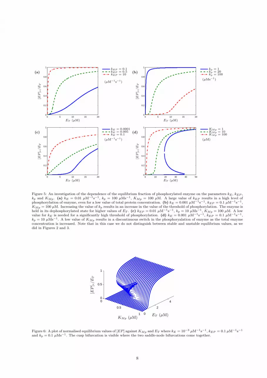
We now demonstrate how the behaviour of the system depends on the values of kE , kEP , kp and KMp.This is demonstrated in the plots of the equilibrium values of [EP ] in Figure 5. In Figures 5 (a), (b) and(c), a high value of kp or a low value of either kE or kEP results in a low threshold for phosphorylation andvice versa. Figure 5 (d) shows that if kE , kEP and kp are held fixed, a sufficiently low value of KMp resultsin a discontinuous switch. Note that in order for the phosphorylation of enzyme to be suppressed for lowconcentrations of total enzyme, kE should be less than kEP .
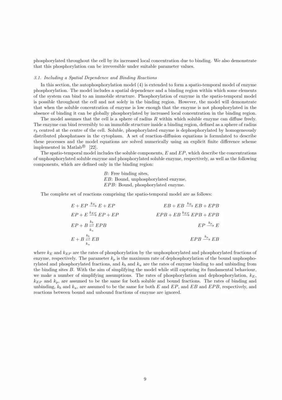
Figure 6 demonstrates that a relatively low value of KMp results in the equation F ([EP ]) = 0 havingthree real roots for a range of values of ET and the system displays the discontinuous switch behaviour.Increasing the value of KMp sufficiently results in a change to a continuous switch. This is the hallmark of acusp bifurcation that acts as an organising centre for the two branches of saddle-node bifurcations and thusfor the type of switch (continuous or discontinuous) the system displays.
3. A Spatio-Temporal Autophosphorylation Model
In this section we develop a mathematical model of autophosphorylation that includes a spatial depen-dence and binding reactions. We use this model to demonstrate how an enzyme can become significantly
6

0 2 4 6 8 100
0.2
0.4
0.6
0.8
1
[EP] e/E
T
ET (µM)
(a)
0 100 200 300 4000
0.2
0.4
0.6
0.8
1
[EP]/E
T
(b)
t (min)
ET = 1 µMET = 2 µMET = 3 µM
0 5 10 15 200
0.2
0.4
0.6
0.8
1
[EP]/E
T
(c)
t (min)
ET = 10 µMET = 20 µMET = 50 µM
Figure 4: A plot of the normalised equilibrium values against ET and time plots of the phosphorylated fraction of enzyme forvarious values of ET . In each plot, kE = 10−5 µM−1s−1, kEP = 10−3 µM−1s−1, kp = 0.1 µMs−1 and KMp = 100 µM. (a)The given set of parameter values results in a continuous switch for the equilibrium values. (b) In this case [EP ](t = 0) = 0and ET takes a number of relatively low values. (c) In this case [EP ](t = 0) = 0 and ET takes various, relatively high values.
7
0 5 10 15 200
0.2
0.4
0.6
0.8
1
ET (µM)
[EP] e/E
T
(a)kEP = 0.1kEP = 0.5kEP = 10
(µM−1s−1)
0 5 10 15 200
0.2
0.4
0.6
0.8
1
ET (µM)
[EP] e/E
T
(b)kp = 1kp = 20kp = 100
(µMs−1)
0 5 10 15 200
0.2
0.4
0.6
0.8
1
ET (µM)
[EP] e/E
T
(c)kE = 0.0001kE = 0.005kE = 0.1
(µM−1s−1)
0 10 20 30 40 500
0.2
0.4
0.6
0.8
1
ET (µM)
[EP] e/E
T
(d)KMp = 1KMp = 10KMp = 100
(µM)
Figure 5: An investigation of the dependence of the equilibrium fraction of phosphorylated enzyme on the parameters kE , kEP ,kp and KMp. (a) kE = 0.01 µM−1s−1, kp = 100 µMs−1, KMp = 100 µM. A large value of kEP results in a high level ofphosphorylation of enzyme, even for a low value of total protein concentration. (b) kE = 0.001 µM−1s−1, kEP = 0.1 µM−1s−1,KMp = 100 µM. Increasing the value of kp results in an increase in the value of the threshold of phosphorylation. The enzyme isheld in its dephosphorylated state for higher values of ET . (c) kEP = 0.01 µM−1s−1, kp = 10 µMs−1, KMp = 100 µM. A lowvalue for kE is needed for a significantly high threshold of phosphorylation. (d) kE = 0.001 µM−1s−1, kEP = 0.1 µM−1s−1,kp = 10 µMs−1. A low value of KMp results in a discontinuous switch in the phosphoryalation of enzyme as the total enzymeconcentration is increased. Note that in this case we do not distinguish between stable and unstable equilibrium values, as wedid in Figures 2 and 3.
0
0.5
1 0
2
40
0.5
1
ET (µM)
[EP] e/E
T
KMp (µM)
Figure 6: A plot of normalised equilibrium values of [EP ] againstKMp and ET where kE = 10−3 µM−1s−1, kEP = 0.1 µM−1s−1
and kp = 0.1 µMs−1. The cusp bifurcation is visible where the two saddle-node bifurcations come together.
8
phosphorylated throughout the cell by its increased local concentration due to binding. We also demonstratethat this phosphorylation can be irreversible under suitable parameter values.
3.1. Including a Spatial Dependence and Binding Reactions
In this section, the autophosphorylation model (4) is extended to form a spatio-temporal model of enzymephosphorylation. The model includes a spatial dependence and a binding region within which some elementsof the system can bind to an immobile structure. Phosphorylation of enzyme in the spatio-temporal modelis possible throughout the cell and not solely in the binding region. However, the model will demonstratethat when the soluble concentration of enzyme is low enough that the enzyme is not phosphorylated in theabsence of binding it can be globally phosphorylated by increased local concentration in the binding region.
The model assumes that the cell is a sphere of radius R within which soluble enzyme can diffuse freely.The enzyme can bind reversibly to an immobile structure inside a binding region, defined as a sphere of radiusrb centred at the centre of the cell. Soluble, phosphorylated enzyme is dephosphorylated by homogeneouslydistributed phosphatases in the cytoplasm. A set of reaction-diffusion equations is formulated to describethese processes and the model equations are solved numerically using an explicit finite difference schemeimplemented in Matlab R© [22].
The spatio-temporal model includes the soluble components, E and EP , which describe the concentrationsof unphosphorylated soluble enzyme and phosphorylated soluble enzyme, respectively, as well as the followingcomponents, which are defined only in the binding region:
B: Free binding sites,EB: Bound, unphosphorylated enzyme,EPB: Bound, phosphorylated enzyme.
The complete set of reactions comprising the spatio-temporal model are as follows:
E + EPkE−→ E + EP EB + EB
kE−→ EB + EPB
EP + EkEP−→ EP + EP EPB + EB
kEP−→ EPB + EPB
EP +Bkb
⇄
ku
EPB EPkp
−→ E
E +Bkb
⇄ku
EB EPBkp
−→ EB
where kE and kEP are the rates of phosphorylation by the unphosphorylated and phosphorylated fractions ofenzyme, respectively. The parameter kp is the maximum rate of dephosphorylation of the bound unphospho-rylated and phosphorylated fractions, and kb and ku are the rates of enzyme binding to and unbinding fromthe binding sites B. With the aim of simplifying the model while still capturing its fundamental behaviour,we make a number of simplifying assumptions. The rates of phosphorylation and dephosphorylation, kE ,kEP and kp, are assumed to be the same for both soluble and bound fractions. The rates of binding andunbinding, kb and ku, are assumed to be the same for both E and EP , and EB and EPB, respectively, andreactions between bound and unbound fractions of enzyme are ignored.
9

The partial differential equations describing the model reactions are as follows:
∂[E]
∂t=
D
r2∂
∂r
(
r2∂[E]
∂r
)
− kb[E][B] + ku[EB]
− kE [E]2 − kEP [E][EP ] +kp[EP ]
KMp + [EP ],
∂[EP ]
∂t=
D
r2∂
∂r
(
r2∂[EP ]
∂r
)
− kb[EP ][B] + ku[EPB]
+ kE [E]2 + kEP [E][EP ]−kp[EP ]
KMp + [EP ],
∂[EB]
∂t= kb[E][B]− ku[EB]− kE [EB]2
− kEP [EB][EPB] +kp[EPB]
KMp + [EPB],
∂[EPB]
∂t= kb[EP ][B]− ku[EPB] + kE [EB]2
+ kEP [EB][EPB]−kp[EPB]
KMp + [EPB],
∂[B]
∂t= −kb[EP ][B]− kb[E][B] + ku[EPB] + ku[EB],
(6)
where, similar to Section 2, [E] = [E](r, t), [EP ] = [EP ](r, t), [EB] = [EB](r, t), [EPB] = [EPB](r, t)and [B] = [B](r, t) refer to the concentrations of E, EP , EB, EPB and B, respectively. The parameterskb = kb(r) and ku = ku(r) are dependent on r. The forms chosen for kb and ku can be found in Section 3.2.The parameter D is the coefficient of diffusion, which is assumed to be constant and the same for both Eand EP .
3.2. Parameter Values for the Spatio-Temporal Model
A number of sample parameter values are taken for the spatio-temporal model, many of which are typicalvalues for several enzymes. These are now discussed and all the values that we assume are displayed in Table2. We take the range 0.1 − 1000 µM as a suitable range for enzyme concentrations [23]. It is assumed thatthe enzyme is initially homogeneously distributed throughout the cell with a concentration ET .
A range of values for kE and kEP are considered, based on the values given before in Table 1. Theparameters kE and kEP are both of the form kcat/KM and, hence, a range of values of 10−3 − 103 µM−1s−1
is considered for them. However, in order for the soluble enzyme to be effectively phosphorylated due to anincrease in concentration in the binding region, kEP should take a larger value than kE . A concentration of0.1− 10 µM is typical for many phosphatases [20, 21]. The parameter kp is of the form kcat[P ], and hence, arange of values of 0.1− 1000 µMs−1 is considered for kp.
As motivation for our choices of parameters for binding, we consider the Aurora B system, in whichAurora B, an autophosphorylating protein, binds to centromeres in mitosis. We assume that the bindingregion has a radius of rb = 300 nm. This is about half the total width of a biorientated centromere in mitosis[24, 25]. We assume that BT can take a maximum value of 104 µM. Values for the rate of protein binding,kb, vary significantly [26]. However, a typical rate of specific binding to DNA is 0.1− 1 µM−1s−1 [27, 28, 29].Based on these results we assume that
kb =
{
1 µM−1s−1 for r ≤ rb
0 for rb < r ≤ R(7)
Aurora B has a rate of unbinding of 0.01 s−1 [30, 31]. Hence, we assume that
ku =
{
0.01 s−1 for r ≤ rb
0 for rb < r ≤ R(8)
10
Parameter Description Estimate
kE , kEP Rates of phosphorylation 10−3 − 103 µM−1s−1
kp Rate of dephosphorylation 0.1− 1000 µMs−1
KMp Half-saturation constant for de-phosphorylation
0.1− 1000 µM
ET Total enzyme concentration 0.1− 1 µMBT Total binding site concentration < 104 µM
kb Rate of binding
{
0.1− 1 µM−1s−1 if r ≤ rb
0 µM−1s−1 if rb < r ≤ R
ku Rate of unbinding
{
0.01 s−1 if r ≤ rb
0 s−1 if rb < r ≤ R
R Cellular radius 5 µmrb Binding region radius 300 nmD Diffusion coefficient 1− 15 µm2s−1
Table 2: Parameter values for the spatio-temporal autophosphorylation model.
3.3. Analysis of the Spatio-Temporal Model
The spatio-temporal model introduced in Section 3.1 is solved numerically using a finite difference schemeimplemented in Matlab. An explicit scheme with forward differences in time and central differences in spacewas used. The initial conditions chosen for the simulations are
[E](r, t = 0) = ET for 0 ≤ r ≤ R, [EP ](r, t = 0) = 0 for 0 ≤ r ≤ R,
[EB](r, t = 0) = 0 for 0 ≤ r ≤ R, [EPB](r, t = 0) = 0 for 0 ≤ r ≤ R,
[B](r, t = 0) =
{
BT for 0 ≤ r ≤ rb
0 for rb < r ≤ R,
and the boundary conditions are
∂[E]
∂r(r = 0, t) = 0,
∂[EP ]
∂r(r = 0, t) = 0,
∂[E]
∂r(r = R, t) = 0,
∂[EP ]
∂r(r = R, t) = 0,
for t > 0. It was shown in Section 2 that, for the autophosphorylation model (4), the concentration of an au-tophosphorylated enzyme must be above a threshold concentration in order to be effectively phosphorylated.In order for the enzyme to remain unphosphorylated at relatively low concentration in the cytoplasm in theabsence of binding its soluble concentration must be below such a threshold. Increased local concentrationdue to binding can then result in phosphorylation of the enzyme following a continuous or discontinuousswitch as shown in Figure 7. This figure shows two representative plots of equilibrium values that wouldbe feasible candidates for the autophosphorylation of soluble enzyme due to binding. Both diagrams have asuitable threshold for phosphorylation that is higher than many typical cellular enzyme concentrations.
Note that the discontinuous switch can for all practical purposes be considered here to be irreversiblein the context of the real system. For example, if the soluble concentration of enzyme is in the region inwhich [EP ] has three equilibrium points and the enzyme is maintained in its dephosphorylated state, anincrease of ET past the bifurcation point due to localisation of the protein results in a switch to a high levelof phosphorylation. If ET is then lowered, such that it returns to the initial value of the soluble concentrationof enzyme, this level of phosphorylation of enzyme is maintained. In other words, increasing the concentrationof enzyme past a threshold for phosphorylation can result in an effectively irreversible phosphorylation of thekinase.
11
0 10 20 30 40 500
0.2
0.4
0.6
0.8
1
ET (µM)
(a)
[EP] e/E
T
0 2 4 6 8 100
0.2
0.4
0.6
0.8
1
ET (µM)
(b)
[EP] e/E
T
Figure 7: Plots of the equilibrium phosphorylated fraction of enzyme as a function of the concentration of total enzyme. Theplots here are the equilibrium solutions of (4). These exhibit typical responses that are necessary for the enzyme to remaindephosphorylated at suitably low soluble concentrations but to become phosphorylated due to concentration by binding. (a)Enzyme phosphorylation may follow a continuous switch. The parameters for this plot are kE = 10−4 µM−1s−1, kEP =0.01 µM−1s−1, kp = 10 µMs−1 and KMp = 100 µM. (b) The enzyme may be phosphorylated via a discontinuous switch dueto concentration. In this case, kE = 10−3 µM−1s−1, kEP = 10 µM−1s−1, kp = 10 µMs−1 and KMp = 0.1 µM.
3.3.1. The Model Demonstrates Phosphorylation of Soluble Enzyme Due to Increased Local Concentration
In order to maintain a significant phosphorylation of soluble enzyme, the rate of dephosphorylationshould be low enough that enzyme that is activated in the binding region is not dephosphorylated quicklyafter returning to soluble concentrations. Also, if the phosphorylation of soluble enzyme is to be the result ofan increase in local concentration, then the rates of phosphorylation should be low enough that the solubleenzyme remains dephosphorylated in the absence of binding. The analysis in Section 2 suggests that in orderfor the phosphorylation of the enzyme to be suppressed at typical soluble concentrations kE should be muchless than kEP . In this case, the phosphorylated fraction of enzyme, EP , contributes to phosphorylation muchmore than the dephosphorylated fraction, E, does.
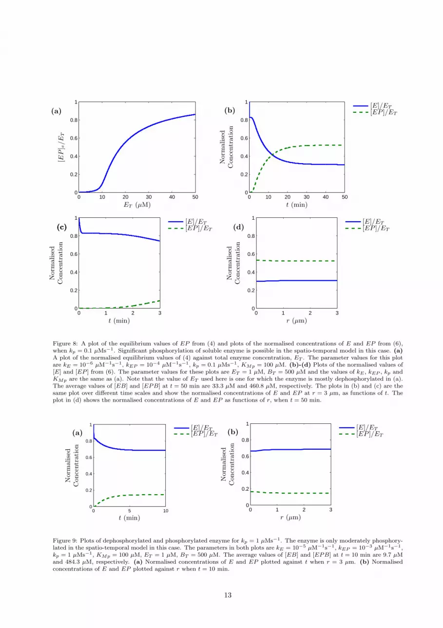
In Figure 8 (a), equilibrium values of (4) are plotted which show a continuous switch and it can be seenin this case that enzyme phosphorylation is suppressed for concentrations below 10 µM. In Figures 8 (b)-(d),[E]/ET and [EP ]/ET from (6) are plotted, using the same reaction rates as Figure 8 (a). In these cases,the initial soluble concentration of total protein, ET , is 1 µM, below the threshold for phosphorylation, asevidenced by Figure 8 (a). Figures 8 (b) and (c) show the normalised values of [E] and [EP ] at r = 3 µm.Figure 8 (c) shows clearly the change in soluble enzyme levels over the first three minutes. Initially, thereis a rapid drop in the concentration of total soluble enzyme due to binding. This is followed by a lag inthe phosphorylation of soluble enzyme due to the relatively slow dynamics of phosphorylation in the bindingregion. After 30 minutes, a significant fraction of soluble enzyme is phosphorylated throughout the cell, asseen in Figure 8 (d). Note that in Figure 8, the value of kEP is 10−4 µM−1s−1. This is lower than the typicalrate of an enzyme catalysed reaction of 10−3 − 1 µM−1s−1 [16].
3.3.2. Soluble Enzyme can be Phosphorylated when the rate of Phosphatase Activity is Low
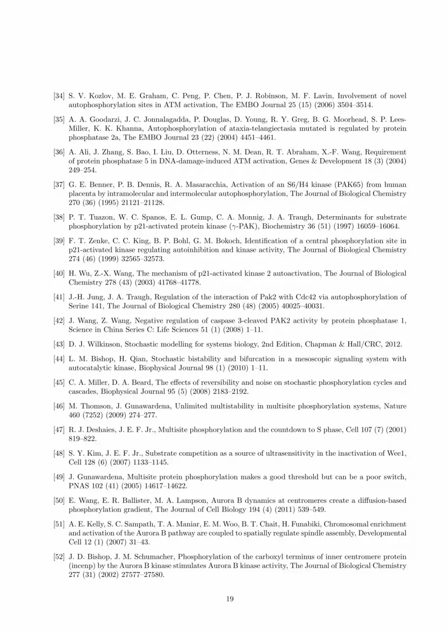
The parameter values in Figure 9 are the same as Figure 8, except the values of kE , kEP and kp are alllarger by a factor of 10. This does not change the profile of the plot of the equilibrium values, which is shownin Figure 8 (a). If kE , kEP and kp in (4) are all changed by the same factor then the equilibrium values of[EP ] remain unchanged, which is clear upon examination of (4). In the case where the values of kE , kEP
and kp are all larger by a factor of 10, the dynamics are much faster, as seen in Figure 9 (a), when comparedwith Figure 8 (b). These faster dynamics result in less phosphorylation of soluble enzyme at equilibrium,shown in Figure 9 (b), when compared with Figure 8 (d).
The soluble enzyme can be substantially phosphorylated in the model throughout the cytoplasm in adiffusion dependent manner if kp = 0.1 µMs−1, as in Figure 8, and can be phosphorylated at a moderatelevel if kp = 1 µMs−1, as in Figure 9. In both of these figures, KMp = 100 µM, meaning the first orderrate constants (kp/KMp) for the dephosphorylation reactions are 10−3 s−1 and 0.01 s−1 in Figures 8 and 9,
12
0 10 20 30 40 500
0.2
0.4
0.6
0.8
1
(a)
[EP] e/E
T
ET (µM)0 10 20 30 40 50
0
0.2
0.4
0.6
0.8
1
(b)[E]/ET
[EP ]/ET
t (min)
Norm
alised
Concentration
0 1 2 30
0.2
0.4
0.6
0.8
1
(c)(c)(c)[E]/ET
[EP ]/ET
t (min)
Norm
alised
Concentration
0 1 2 30
0.2
0.4
0.6
0.8
1
(d) [EP ]/ET
[E]/ET
r (µm)
Norm
alised
Concentration
Figure 8: A plot of the equilibrium values of EP from (4) and plots of the normalised concentrations of E and EP from (6),when kp = 0.1 µMs−1. Significant phosphorylation of soluble enzyme is possible in the spatio-temporal model in this case. (a)A plot of the normalised equilibrium values of (4) against total enzyme concentration, ET . The parameter values for this plotare kE = 10−6 µM−1s−1, kEP = 10−4 µM−1s−1, kp = 0.1 µMs−1, KMp = 100 µM. (b)-(d) Plots of the normalised values of[E] and [EP ] from (6). The parameter values for these plots are ET = 1 µM, BT = 500 µM and the values of kE , kEP , kp andKMp are the same as (a). Note that the value of ET used here is one for which the enzyme is mostly dephosphorylated in (a).The average values of [EB] and [EPB] at t = 50 min are 33.3 µM and 460.8 µM, respectively. The plots in (b) and (c) are thesame plot over different time scales and show the normalised concentrations of E and EP at r = 3 µm, as functions of t. Theplot in (d) shows the normalised concentrations of E and EP as functions of r, when t = 50 min.
0 5 100
0.2
0.4
0.6
0.8
1
(a)[E]/ET[EP ]/ET
t (min)
Norm
alised
Concentration
0 1 2 30
0.2
0.4
0.6
0.8
1
(b)[E]/ET
[EP ]/ET
Norm
alised
Concentration
r (µm)
Figure 9: Plots of dephosphorylated and phosphorylated enzyme for kp = 1 µMs−1. The enzyme is only moderately phosphory-lated in the spatio-temporal model in this case. The parameters in both plots are kE = 10−5 µM−1s−1, kEP = 10−3 µM−1s−1,kp = 1 µMs−1, KMp = 100 µM, ET = 1 µM, BT = 500 µM. The average values of [EB] and [EPB] at t = 10 min are 9.7 µMand 484.3 µM, respectively. (a) Normalised concentrations of E and EP plotted against t when r = 3 µm. (b) Normalisedconcentrations of E and EP plotted against r when t = 10 min.
13

0 2 4 6 8 100
0.2
0.4
0.6
0.8
1
(a)
[EP] e/E
T
ET (µM)0 5 10 15
0
0.2
0.4
0.6
0.8
1
Norm
alised
Concentration
t (min)
(b)[E]/ET
[EP ]/ET
0 1 2 30
0.2
0.4
0.6
0.8
1
Norm
alised
Concentration
r (µm)
(c)[E]/ET
[EP ]/ET
Figure 10: A plot of scaled equilibrium values of EP and plots of the normalised concentrations of E and EP demonstratingthe case where the phosphorylation of soluble enzyme by concentration is irreversible. In each of these plots, the parametersare kE = 10−6 µM−1s−1, kEP = 0.01 µM−1s−1, kp = 0.01 µMs−1, KMp = 0.1 µM. (a) A plot of scaled equilibrium valuesof (4). (b) This plot shows the normalised concentrations of both fractions of soluble enzyme for r = 3 µm, ET = 6 µM andBT = 500 µM. In this plot, kb takes a value of 0, instead of 1 µM−1s−1 after t = 8 min which is indicated by the verticaldashed-dotted line. Note that the value of ET = 6 µM is one for which the plot in (a) has three values. (c) This plot shows thenormalised concentrations of both fractions of soluble enzyme as a function of r under the same set of parameters as (b) whent = 6 min and the system is at steady state.
respectively.
3.3.3. Phosphorylation of Soluble Enzyme can be Irreversible
The simulations displayed in Figure 10 demonstrate that phosphorylation of soluble enzyme in the two-step model can be irreversible for a suitable choice of parameter values. Figure 10 (a) shows a plot of scaledequilibrium values of phosphorylated enzyme for which [EP ]e can take one of three equilibrium values fora suitable range of ET values. In Figures 10 (b) and (c), solutions of the two-step model in space andtime demonstrate that choosing ET = 6 µM results in significant phosphorylation of the enzyme throughoutthe cytoplasm. In Figure 10 (b), it is demonstrated that this phosphorylation is indeed irreversible. Att = 8 min, indicated by the vertical dashed-dotted line, the rate of enzyme binding, kb, is given a value of 0.The enzyme remains phosphorylated throughout the cytoplasm despite the fact that binding in the modelhas been switched off.
4. Discussion
In this section, we first discuss the model of autophosphorylation presented in Section 2. Following this,we discuss the spatio-temporal model of enzyme autophosphorylation described in Section 3. Finally, wemake some concluding statements.
14

4.1. The Solely Time-Dependent Model of Intermolecular Autophosphorylation
The model of autophosphorylation in Section 2 provides a mathematical description of a common motifin cellular biology. Here, we give a brief summary of results followed by a discussion of possible extensionsand modifications of the model.
4.1.1. A Generic Model of Intermolecular Autophosphorylation
The model of autophosphorylation in Section 2 includes phosphyorylation by both the unphosphorylatedand phosphorylated fractions of enzyme, as well as dephosphorylation by an enzyme of constant concentration.This results in a model of autophosphorylation where the total concentration of enzyme is an important factorin determining the fraction of the enzyme that is phosphorylated at steady state.
The inclusion of phosphatase activity in the model suppresses the phosphorylation of enzyme for a rangeof values of the concentration of total enzyme. The model also demonstrates that a discontinuous switch ispossible, due to the effect of the phosphatase, where an increase in total enzyme concentration can result ina rapid switch to a high level of phosphorylated enzyme at steady state.
Model simulations demonstrate that a lag in the phosphorylation of enzyme may exist whereby theenzyme remains in its dephosphorylated state for a period of time before there is a noticeable change inits phosphorylation level. This results in a sigmoidal concentration profile of phosphorylated enzyme as afunction of time, which is typical of autophosphorylation reactions. Model simulations also demonstratethat autophosphorylation can proceed more rapidly for some parameter regimes, with no noticeable lag inphosphorylation, and that the rate of autophosphorylation is dependent on the total enzyme concentration.
4.1.2. The Model may be Extended and Adapted
The model in Section 2 can be extended to include effects that may be a common feature of manyautophosphorylation systems and the effects of extra components in the modelling may be investigated. Forexample, the intermediate step of phosphodonor binding (which is incorporated here in the rate constantskE and kEP ) could be explicitly included in the model, as in the model of Wang and Wu [15]. Incorporatingthe concentration of phosphodonor as a dynamic variable can be used to examine the effect of saturation ofbinding to the phosphodonor. Another possible extension of the model could be the inclusion of a distinctsignalling protein that initiates autophosphorylation of the enzyme, as is the case in the model of Creager-Allen et al. [13], where Ca2+ is necessary for the autoactivation of CaMKII. Similarly, inhibition of enzymeautophosphorylation could be included.
Although the model of autophosphorylation in Section 2 does not attempt to model any particular systemexplicitly, it can improve our understanding of a number of systems that are known to include autophos-phorylation and phosphatase-mediated dephosphorylation. Examples include Myosin IIIa [32, 33] (a motorprotein that binds actin and localises to filopodial tips), Ataxia Telangiectasia Mutated (ATM) Kinase[7, 34, 8, 35, 36] (an enzyme that is activated by DNA double-strand breaks), and p21 Activated Kinase 2(PAK2) [37, 38, 39, 40, 41, 42] (a protein that responds to several stress signals). In order to model anyone of these systems explicitly, it may be necessary to incorporate other reactions specific to the system inquestion.
4.1.3. Stochastic Switches
The model presented in Section 2 is deterministic which is an appropriate approach when studying largemolecule numbers where stochastic effects can be ignored. However, stochastic models may also be ableto produce the results presented in Section 2. Although similar stochastic and deterministic models mayaccurately describe the same phenomena, for small protein numbers, a stochastic model may exhibit differentqualitative behaviour to a deterministic model [43]. In Section 2, it was shown that a discontinuous switchresults from a cubic expression for the equilibrium values of phosphorylated enzyme due to the nonlineareffects of phosphatase activity. However, Bishop and Qian [44] have shown that it is possible for a similarstochastic system to result in a discontinuous switch when the nonlinearity is merely quadratic. Othergroups have described similar stochastic switches, such as Miller and Beard [45] for a phosphorylation-dephosphorylation cycle.
15

4.2. The Spatio-Temporal Model of Enzyme Autophosphorylation
In Section 3, we incorporated a spatial dependence in our model of autophosphorylation and provided aproof-of-concept of how it is possible for an autophosphorylating enzyme to become phosphorylated through-out the cell by its increased local concentration. We now discuss the results of the model and consider possibleextensions of it.
4.2.1. The Modelling Improves Our Understanding of the Process
The model in Section 3 demonstrates that enzyme phosphorylation can be suppressed in the cytoplasmby phosphatase activity, as long as the rates of phosphorylation are sufficiently low. The enzyme can bephosphorylated throughout the cytoplasm in a diffusion-dependent manner by its concentration at bindingsites. In the modelling, this is achieved by choosing a sufficiently low value for the pseudo first-order rate ofphosphatase activity, kp/KMp.
It may also be possible to describe a similar cellular phosphorylation of enzyme due to localised con-centration using different models. For example, a model in which the phosphorylation of soluble enzyme issuppressed by phosphatase activity, as in the model in Section 3, but the binding of phosphatases at a specificcellular location leads to a lower soluble phosphatase concentration thereby enabling the initiation of globalenzyme phosphorylation.
Phosphorylation of soluble enzyme in the model in Section 3 can sometimes be effectively irreversibleunder suitable conditions, if there is a discontinuous switch involved in the phosphorylation of the enzyme.In the mathematical model, the enzyme can be irreversibly phosphorylated if the concentration of totalprotein is within a relatively narrow range of values. It is not known how robust an irreversible mechanismmay be, since it would need to be ensured that the soluble enzyme concentration is maintained within aspecific range. However, the inclusion of other processes, such as multisite phosphorylation, may resultin a model that demonstrates a robust irreversible phosphorylation mechanism for a wide range of solubleconcentrations. Multisite phosphorylation has been studied from a dynamical systems point of view in manydifferent systems and, generally, the inclusion of multisite phosphorylation leads to increased robustness andflexibility [46] and can also lead to higher thresholds for activation and lower thresholds for deactivation[47, 48, 49].
4.2.2. The Modelling Can Be Adapted to Model Specific Systems
The mathematical model in Section 3 can help us to understand the general process of global activation dueto localised concentration of a generic enzyme. Although this is a generic model it may be adapted or extendedin order to describe many specific biological systems, for example by the incorporation of extra reactions orby using different parameter values or the use of a different model geometry. The autophosphorylationof a protein due to its increased local concentration has been hypothesised in a number of systems. Forexample, Aurora B kinase (a protein that plays multiple important roles in mitotic processes) has beenobserved to activate throughout the cell in a diffusion-dependent manner due to its increased concentrationat centromeres [50]. However, the phosphorylation reactions that result in the full activation of Aurora B aremore complex than presented in Section 3 as the kinase is phosphorylated on more than one site [10, 51, 52].Another example is ATM kinase, mentioned in Section 4.1.2. This kinase exerts an influence on globalcellular dynamics in response to its increased local concentration at DNA double-strand breaks [7]. However,this kinase is also autophosphorylated on multiple sites [34, 8]. Myosin IIIa, briefly mentioned in Section4.1.2, is phosphorylated by its increased concentration [32, 33]. However, as its concentration is increasedat filopodial tips, a relatively small region, the model geometry used in Section 3 is not appropriate. Also,the phosphorylation of Myosin IIIa affects its actin binding affinity [32, 33], and due to this its filopodiallocalisation, and this may have to be incorporated in a successful model.
4.3. Concluding Remarks
Autophosphorylation is a mechanism that is involved in the regulation of several cellular enzymes andthus has a role to play in many biological functions. The models of intermolecular autophosphorylationpresented here demonstrate the importance of dephosphorylation in the behaviour of autophosphorylatingproteins and provide insight into the process of spatial activation by localised concentration. They may alsofind use in modelling systems in which there is concentration-dependent activation, either due to a global orlocal change in concentration. There is ample scope to extend the models introduced here to describe otherspecific molecular biological systems.
16

Acknowledgements
Kevin Doherty was supported in this work by the College of Science, National University of Ireland,Galway. Martin Meere thanks the National University of Ireland, Galway for the award of a travel grant.
[1] C. A. Dodson, S. Yeoh, T. Haq, R. Bayliss, A kinetic test characterizes kinase intramolecular andintermolecular autophosphorylation mechanisms, Science Signaling 6 (282).
[2] J. A. Smith, S. H. Francis, J. D. Corbin, Autophosphorylation: a salient feature of protein kinases,Molecular and Cellular Biochemistry 127-128 (1) (1993) 51–70.
[3] S. R. Hubbard, Protein tyrosine kinases: autoregulation and small-molecule inhibition, Current Opinionin Structural Biology 12 (6) (2002) 735–741.
[4] W. J. Gullick, J. Downward, M. D. Waterfield, Antibodies to the autophosphorylation sites of epidermalgrowth factor receptor protein-tyrosine kinase as probes of structure and function, The EMBO Journal4 (11) (1985) 2869–2877.
[5] J. Downward, P. Parker, M. D. Waterfield, Autophosphorylation sites on the epidermal growth factorreceptor, Nature 311 (5985) (1984) 483–485.
[6] A. M. Honegger, R. M. Kris, A. Ullrich, J. Schlessinger, Evidence that autophosphorylation of solubilizedreceptors for epidermal growth factor is mediated by intermolecular cross-phosphorylation, Proceedingsof the National Academy of Sciences of the United States of America 86 (1989) 925–929.
[7] C. J. Bakkenist, M. B. Kastan, DNA damage activates ATM through intermolecular autophosphorylationand dimer dissociation, Nature 421 (6922) (2003) 499–506.
[8] S. V. Kozlov, M. E. Graham, B. Jakob, F. Tobias, A. W. Kijas, M. Tanuji, P. Chen, P. J. Robinson,G. Taucher-Scholz, K. Suzuki, S. So, D. Chen, M. F. Lavin, Autophosphorylation and ATM activation:additional sites add to the complexity, The Journal of Biological Chemistry 286 (11) (2011) 9107–9119.
[9] S. So, A. J. Davis, D. J. Chen, Autophosphorylation at serine 1981 stabilizes ATM at DNA damagesites, The Journal of Cell Biology 187 (7) (2009) 977–990.
[10] Y. Yasui, T. Urano, A. Kawajiri, K. ichi Nagata, M. Tatsuka, H. Saya, K. Furukawa, T. Takahashi,I. Izawa, M. Inagaki, Autophosphorylation of a newly identified site of Aurora-B is indispensible forcytokinesis, The Journal of Biological Chemistry 279 (13) (2004) 12997–13003.
[11] L. G. DeFazio, R. M. Stansel, J. D. Griffith, G. Chu, Synapsis of DNA ends by DNA-dependent proteinkinase, The EMBO Journal 21 (12) (2002) 2843–3212.
[12] F. Wang, J. Dai, J. R. Daum, E. Niedzialkowska, B. Banerjee, P. T. Stukenberg, G. J. Gorbsky, J. M. G.Higgins, Histone H3 Thr-3 phosphorylation by Haspin postition Aurora B at centromeres in mitosis,Science 330 (6001) (2010) 231–235.
[13] R. L. Creager-Allen, R. E. Silversmith, R. B. Bourret, A link between dimerization and autophosphory-lation of the response regulator PhoB, The Journal of Biological Chemistry 288 (2013) 21755–21769.
[14] H. Okamoto, K. Ichikawa, Switching characteristics of a model for biochemical-reaction networks de-scribing autophosphorylation versus dephosphorylation of Ca2+/calmodulin-dependent protein kinaseII, Biological Cybernetics 82 (1) (2000) 35–47.
[15] Z.-X. Wang, J.-W. Wu, Autophosphorylation kinetics of protein kinases, Biochemical Journal 368 (2002)947–952.
[16] A. Bar-Even, E. Noor, Y. Savir, W. Liebermeister, D. Davidi, D. S. Tawfik, R. Milo, The moderatelyefficent enzyme: Evolutionary and physicochemical trends shaping enzyme parameters, Biochemistry50 (21) (2011) 4402 –4410.
17

[17] A. Honegger, T. J. Dull, D. Szapary, A. Komoriya, R. Kris, A. Ullrich, J. Schlessinger, Kinetic parametersof the protein tyrosine kinase activity of EGF-receptor mutants with individually altered autophospho-rylation sites, The EMBO Journal 7 (10) (1988) 3053–3060.
[18] P. Stralfors, A. Hiraga, P. Cohen, The protein phosphatases involved in cellular regulation: Purificationand characterisation of the glycogen-bound form of protein phosphatase-1 from rabbit skeletal muscle,European Journal of Biochemistry 149 (2) (1985) 295–303.
[19] N. K. Tonks, P. Cohen, The protein phosphatases involved in cellular regulation: Identification of theinhibitor-2 phosphatases in rabbit skeletal muscle, European Journal of Biochemistry 145 (1) (1984)65–70.
[20] B. Schwanhausser, D. Busse, N. Li, G. Dittmar, J. Schuchhardt, J. Wolf, W. Chen, M. Selbach, Globalquantification of mammalian gene expression control, Nature 473 (7347) (2011) 337–342.
[21] H. L. Tung, T. J. Resink, B. A. Hemmings, S. Shenolikar, P. Cohen, The catalytic subunits of proteinphosphatase-1 and protein phosphatase 2a are distinct gene products, European Journal of Biochemistry138 (3) (1984) 635–641.
[22] MATLAB, version 7.10.0 (R2010a), The MathWorks Inc., Natick, Massachusetts, 2010.
[23] K. R. Albe, M. H. Butler, B. E. Wright, Cellular concentrations of enzymes and their substrates, TheJournal of Theoretical Biology 143 (2) (1990) 163–195.
[24] D. Liu, G. Vader, M. J. M. Vromans, M. A. Lampson, S. M. A. Lens, Sensing chromosome bi-orientationby spatial separation of Aurora B kinase from kinetochore substrates, Science 323 (5919) (2009) 1350–1353.
[25] A. Suzuki, T. Hori, T. Nishino, J. Usukura, A. Miyagi, K. Morikawa, T. Fukagawa, Spindle microtubulesgenerate tension-dependent changes in the distribution of inner kinetochore proteins, The Journal of CellBiology 193 (1) (2011) 125–140.
[26] D. G. Myszka, Kinetic analysis of macromolecular interactions using surface plasmon resonance biosen-sors, Current Opinion in Biotechnology 8 (1) (1997) 50–57.
[27] K. Bondeson, Asa Frostell-Karlsson, L. Fagerstam, G. Magnusson, Lactose repressor-operator DNAinteractions: Kinetic analysis by a surface plasmon resonance biosensor, Analytical Biochemistry 214 (1)(1993) 245–251.
[28] H. K. Binz, P. Amstutz, A. Kohl, M. T. Stumpp, C. Briand, P. Forrer, M. G. Grutter, A. Pluckthun,High-affinity binders selected from designed ankyrin repeat protein libraries, Nature Biotechnology 22 (5)(2004) 575–582.
[29] V. J. B. Ruigrok, E. R. Westra, S. J. J. Brouns, C. Escude, H. Smidt, J. van der Oost, A captureapproach for supercoiled plasmid DNA using a triplex-forming oligonucleotide, Nucleic Acids Research41 (10).
[30] M. Murata-Hori, M. Tatsuka, Y.-L. Wang, Probing the dynamics and functions of Aurora B kinase inliving cells during mitosis and cytokinesis, Molecular Biology of the Cell 13 (4) (2002) 1099–1108.
[31] L. J. Ahonen, A. M. Kukkonen, J. Pouwels, M. A. Bolton, C. D. Jingle, P. T. Stukenberg, M. J. Kallio,Perturbation of Incenp function impedes anaphase chromatid movements and chromosomal passengerprotein flux at centromeres, Chromosoma 118 (1) (2009) 71–84.
[32] O. A. Quintero, J. E. Moore, W. C. Unrath, U. Manor, F. T. Salles, M. Grati, B. Kachar, C. M.Yengo, Intermolecular autophosphorylation regulates Myosin IIIa activity and localization in parallelactin bundles, The Journal of Biological Chemistry 285 (46) (2010) 35770–35782.
[33] O. A. Quintero, W. C. Unrath, S. M. Stevens, U. Manor, B. Kachar, C. M. Yengo, Myosin 3A kinaseactivity is regulated by phosphorylation of the kinase domain activation loop, The Journal of BiologicalChemistry 288 (52) (2013) 37126–37137.
18
[34] S. V. Kozlov, M. E. Graham, C. Peng, P. Chen, P. J. Robinson, M. F. Lavin, Involvement of novelautophosphorylation sites in ATM activation, The EMBO Journal 25 (15) (2006) 3504–3514.
[35] A. A. Goodarzi, J. C. Jonnalagadda, P. Douglas, D. Young, R. Y. Greg, B. G. Moorhead, S. P. Lees-Miller, K. K. Khanna, Autophosphorylation of ataxia-telangiectasia mutated is regulated by proteinphosphatase 2a, The EMBO Journal 23 (22) (2004) 4451–4461.
[36] A. Ali, J. Zhang, S. Bao, I. Liu, D. Otterness, N. M. Dean, R. T. Abraham, X.-F. Wang, Requirementof protein phosphatase 5 in DNA-damage-induced ATM activation, Genes & Development 18 (3) (2004)249–254.
[37] G. E. Benner, P. B. Dennis, R. A. Masaracchia, Activation of an S6/H4 kinase (PAK65) from humanplacenta by intramolecular and intermolecular autophosphorylation, The Journal of Biological Chemistry270 (36) (1995) 21121–21128.
[38] P. T. Tuazon, W. C. Spanos, E. L. Gump, C. A. Monnig, J. A. Traugh, Determinants for substratephosphorylation by p21-activated protein kinase (γ-PAK), Biochemistry 36 (51) (1997) 16059–16064.
[39] F. T. Zenke, C. C. King, B. P. Bohl, G. M. Bokoch, Identification of a central phosphorylation site inp21-activated kinase regulating autoinhibition and kinase activity, The Journal of Biological Chemistry274 (46) (1999) 32565–32573.
[40] H. Wu, Z.-X. Wang, The mechanism of p21-activated kinase 2 autoactivation, The Journal of BiologicalChemistry 278 (43) (2003) 41768–41778.
[41] J.-H. Jung, J. A. Traugh, Regulation of the interaction of Pak2 with Cdc42 via autophosphorylation ofSerine 141, The Journal of Biological Chemistry 280 (48) (2005) 40025–40031.
[42] J. Wang, Z. Wang, Negative regulation of caspase 3-cleaved PAK2 activity by protein phosphatase 1,Science in China Series C: Life Sciences 51 (1) (2008) 1–11.
[43] D. J. Wilkinson, Stochastic modelling for systems biology, 2nd Edition, Chapman & Hall/CRC, 2012.
[44] L. M. Bishop, H. Qian, Stochastic bistability and bifurcation in a mesoscopic signaling system withautocatalytic kinase, Biophysical Journal 98 (1) (2010) 1–11.
[45] C. A. Miller, D. A. Beard, The effects of reversibility and noise on stochastic phosphorylation cycles andcascades, Biophysical Journal 95 (5) (2008) 2183–2192.
[46] M. Thomson, J. Gunawardena, Unlimited multistability in multisite phosphorylation systems, Nature460 (7252) (2009) 274–277.
[47] R. J. Deshaies, J. E. F. Jr., Multisite phosphorylation and the countdown to S phase, Cell 107 (7) (2001)819–822.
[48] S. Y. Kim, J. E. F. Jr., Substrate competition as a source of ultrasensitivity in the inactivation of Wee1,Cell 128 (6) (2007) 1133–1145.
[49] J. Gunawardena, Multisite protein phosphorylation makes a good threshold but can be a poor switch,PNAS 102 (41) (2005) 14617–14622.
[50] E. Wang, E. R. Ballister, M. A. Lampson, Aurora B dynamics at centromeres create a diffusion-basedphosphorylation gradient, The Journal of Cell Biology 194 (4) (2011) 539–549.
[51] A. E. Kelly, S. C. Sampath, T. A. Maniar, E. M.Woo, B. T. Chait, H. Funabiki, Chromosomal enrichmentand activation of the Aurora B pathway are coupled to spatially regulate spindle assembly, DevelopmentalCell 12 (1) (2007) 31–43.
[52] J. D. Bishop, J. M. Schumacher, Phosphorylation of the carboxyl terminus of inner centromere protein(incenp) by the Aurora B kinase stimulates Aurora B kinase activity, The Journal of Biological Chemistry277 (31) (2002) 27577–27580.
19