Some studies on path protection in WDM networks

Photon Netw Commun (2007) 14:165–176DOI 10.1007/s11107-007-0075-0

Some studies on path protection in WDM networks

Yash Aneja · Arunita Jaekel · Subir Bandyopadhyay

Received: 12 October 2006 / Accepted: 8 June 2007 / Published online: 17 July 2007© Springer Science+Business Media, LLC 2007

Abstract Path protection in WDM networks is one of thepopular ways to design resilient WDM networks. Althoughcomplete ILP formulations for optimal design of WDM net-works have been proposed in literature, the computationalcost of actually solving such formulations make this ap-proach impractical, even for moderate sized networks. Thishigh computational cost arises mainly due to the large num-ber of integer variables in the formulations, which increasesthe complexity exponentially. As a result, most practical so-lutions use heuristics, which do not provide any guaranteeson the performance. In this article, we propose two novel ILPformulations, which drastically reduce the number of integervariables compared to existing ILPs. This leads to much moreefficient formulations. We also present a simple heuristic thatmay be used for larger networks for which ILP formulationsbecome computationally intractable.

Keywords WDM Optical networks · Path protection ·ILP · Logical topology · Multihop networks

1 Introduction

The physical topology of an optical network consists of aset of end-nodes (capable of generating data for transmis-sion, receiving data, and having a number of optical trans-mitters and receivers), router nodes, and the optical fibersinterconnecting these nodes. Wavelength division multiple-xing (WDM) divides the huge bandwidth of a fiber into nch

non-overlapping ranges of wavelengths, called WDM chan-nels. The transmission of data from any source node s to

Y. Aneja · A. Jaekel · S. Bandyopadhyay (B)University of Windsor, Windsor, ON, Canada N9B 3P4e-mail: [email protected]

a destination node d uses some carrier wavelength λi andthe modulated optical signal uses the i th channel, for somei, 1 ≤ i ≤ K . A lightpath in a WDM network is a point-to-point communication path that connects a transmitter at s to areceiver at d through a number of router nodes where the en-tire transmission is in the optical domain. We assume the wa-velength continuity constraint so that the lightpath from s to duses the same carrier wavelength λi from s to d on all traver-sed fiber links. The logical topology of a WDM network, is re-presented by a graph GL , where the nodes in GL are the end-nodes in the network and there is a directed edge i → j in GL

(often called a logical edge) from node i to node j , if there is alightpath from node i to node j . A multi-hop WDM networkis one where all pairs of end-nodes are not connected by alogical edge. In such a network, if two end-nodes X and Y arenot connected by a logical edge, to communicate from X to Y ,we need to find a path X → A1 → A2 → · · · → Ak → Y ,such that each edge in the path is a logical edge in the logicaltopology GL corresponding to the network. When we have alogical topology and, a routing strategy to handle the trafficrequest t (s, d) from s to d for all source s and destination d,the congestion of the network is defined as the load on thelogical edge which carries maximum amount of traffic. Someexcellent coverage of these topics may be found in [1–7].

The failure of a single fiber link is the most frequentcause of network failure and may cause all lightpaths usingthe faulty fiber to fail. There are two main approaches forfault management: path protection and restoration [8–21].In restoration, after a failure occurs, we try to find alter-nate routes for all disrupted lightpaths, using any unusedresources. In path protection, for each logical edge, we set uptwo lightpaths—the primary lightpath and the backup light-path, which uses a route through the physical topology thatis fiber-disjoint with respect to the route used by the pri-mary lightpath. The resources for the backup lightpath are

123

166 Photon Netw Commun (2007) 14:165–176

allocated at design time, before any failure has occurred.In the absence of failures, communication uses the primarylightpaths alone. When there is a link failure (for instancedue to a fiber cut), communication that uses the disruptedprimary lightpaths is resumed using the corresponding ba-ckup lightpaths. To reduce the amount of network resourcesreserved for backup lightpaths, shared path protection hasbeen proposed. In this approach, two backup lightpaths areallowed to share a fiber and a channel, if the correspondingprimary lightpaths use routes that are fiber-disjoint [19]. Anumber of exact ILP formulations for the design of survivableWDM networks have been proposed [19, 21–24]. Some heu-ristics for solving the design problem have been presented in[19,21,25].

Given the user requirements for data communication, spe-cified in the form of a traffic matrix T = [t (s, d)] and thecharacteristics of the network, the objective of our formula-tion is to minimize the network congestion by solving thefollowing subproblems:

(1) Determine an optimum logical topology GL for the net-work.

(2) Determine, for each logical edge in GL , an appropriatechannel and a route through the physical topology for aprimary lightpath and a backup lightpath.

(3) Find an optimum routing over the logical topology tohandle the traffic request t (s, d) for all source s and des-tination d.

These subproblems are interrelated since the objective is tominimize the congestion and subproblem 3 cannot be solveduntil subproblem 1 is solved. Subproblem 1 in turn requiressubproblem 2 to be solved in order to ensure that the logicaltopology is indeed realizable.

The logical topology design problem investigated in thisarticle is very similar to the problem proposed in [19]. In[19], the authors propose two formulations ILP1 and ILP2to solve the problem. In order to reduce the computationalcomplexity, the authors make some simplifying assumptions.One important aspect is finding the routes for the primary andthe backup path. In [19] an assumption is made that, whenlooking for a primary or a backup path from a source s toa destination d, it is sufficient to consider R edge-disjointroutes from s to d, for some pre-determined value of R.From these R routes, one will be selected for the primarypath and another one, distinct from the route selected forthe primary path, will be selected for the backup path. Thismeans that for each pair of end-nodes (s, d), edge disjointroutes ρ1(s, d), ρ2(s, d), . . . , ρR(s, d) will be pre-computedbefore solving the formulation. The first approach presentedin [19] (ILP1), solves the logical topology design problem,with the restriction that it examines only R predetermined

routes. The second approach ILP2 makes a further simplifi-cation where the work is done in two phases. Phase I deter-mines the primary paths only while phase II determines thecorresponding backup paths. Clearly, this reduces the com-plexity of the formulation. It is important to note that ILP1itself results in a sub-optimal solution. ILP2 makes furthersimplifications. Since ILP based formulations are intractablefor practical sized networks, the primary motivation for sucha formulation is to be a benchmark for heuristics. Solutionsusing these formulations are not good benchmarks since theyare sub-optimal solutions.

In this article we present two new formulations ILPA andILPB. ILPA does not make any assumptions about the routesfor the primary and the backup paths. In other words, it gua-rantees an optimal solution. It is well known [26] that thecomputational complexity of an ILP is dominated by thenumber of integer variables, which in the case of ILPA andILPB are binary (i.e., 0/1) variables. In terms of the numberof binary variables, ILPA is considerably simpler than bothILP1 and ILP2. ILPB solves the problem under the sameassumptions made for ILP1, so that it not only looks at Rpre-computed routes when determining the primary and thebackup paths but also involves considerably fewer binary va-riables even compared to the ILP2.

We have also proposed a heuristic for larger networks. Thisheuristic also looks at R pre-computed routes as in ILP1 andILP2. An interesting feature of this heuristic is the use of anexisting single commodity network flow algorithm to routetraffic whenever possible.

2 ILP for 1:N protection using a comprehensive search

We will call this formulation ILPA. The approach we usedin ILPA is as follows:

(1) Start with a list L of all possible logical edges in thenetwork. In a network with Ne end-nodes, the list L hasNe(Ne − 1) elements, one for each pair of end-nodes.

(2) Determine GL by selecting logical edges for the net-work, making sure that, for each logical edge in GL , it ispossible to establish a primary and a backup lightpath bysearch all possible routes through the physical topology.

(3) Find an optimum routing over GL for the specified trafficmatrix.

2.1 Notation used

Ne = number of end-nodes in the network.E = the set of all ordered pairs of nodes (i, j) such that i → jis a directed edge in the physical topology.

123

Photon Netw Commun (2007) 14:165–176 167

nch = number of channels permitted on each edge of the net-work.L= the list [�1, �2, . . . , �Ne(Ne−1)] of potential, directed lo-gical edges. Since there is one potential logical edge fromeach source s to each destination d, the number of elementsin L is Ne(Ne − 1).�p = the pth element of L, 1 ≤ p ≤ Ne(Ne − 1).source(p) (destination(p)) = end-node X (Y ) when �p is adirected logical edge X → Y from end-node X to end-nodeY .�max = a continuous variable denoting the congestion of thenetwork.bp = a binary variable for all p, 1 ≤ p ≤ Ne(Ne −1), definedas follows:

bp =⎧⎨

⎩

1 if �p is selected to be included in the logicaltopology,

0 otherwise.

x pe(ype)= a binary variable for the primary (backup) path,used if �p is selected, ∀p, 1 ≤ p ≤ Ne(Ne − 1), defined asfollows:

x pe(ype) =⎧⎨

⎩

1 if �p is selected, and the edge e appears inthe primary (backup) lightpath,

0 otherwise.

wkp(zkp)= a binary variable relevant when �p is selected,∀p, 1 ≤ p ≤ Ne(Ne − 1),∀k, 1 ≤ k ≤ nch , defined asfollows:

wkp(zkp) =⎧⎨

⎩

1 if �p is selected, and the primary (backup)lightpath for �p is allocated channel k,

0 otherwise.

δkpe , γ

kpe , αke, θ

kpe1e2 , and η

kpe are continuous1 variables which

are constrained, using the conditions specified in the ILPbelow to have a value of either 0 or 1 as follows:

δkpe (γ

kpe ) =

⎧⎪⎪⎨

⎪⎪⎩

1 if �p is selected, and the primary (backup)lightpath for �p is allocated channel k andassigned a route containing edge e,

0 otherwise.

αke =

⎧⎪⎪⎨

⎪⎪⎩

1 if there is at least one backup lightpath thatuses edge e and the backup lightpath isallocated channel k,

0 otherwise.

1 It is important to note that we have made extensive use of continuousvariables whose values are constrained to have discrete values. Thistechnique drastically reduces the number of integer variables and hencethe time to solve the MILP formulation.

θkpe1e2 =

⎧⎪⎪⎪⎪⎪⎪⎨

⎪⎪⎪⎪⎪⎪⎩

1 if �p is selected, and the primary lightpathfor �p is assigned a route containing edge e2,the corresponding backup lightpath isassigned a route containing edge e1 and thebackup lightpath is allocated channel k,

0 otherwise.

ηkpe =

⎧⎪⎪⎪⎪⎨

⎪⎪⎪⎪⎩

1 if �p is selected and the route for the primarylightpath for �p uses edge e and thecorresponding backup lightpath is allocatedchannel k,

0 otherwise.

f sdp = a continuous variable denoting the traffic on logical

edge �p from source end-node s to destination end-node d.tku (rk

u )= number of transmitters (receivers) at end-node utuned to the wavelength corresponding to channel k.ε = a very small constant.

For the ease of understanding, we have described the cons-traints for the following formulation in related groups.

2.2 The ILP formulation

The following ILP determines

• a logical topology,• a feasible RWA for the primary and the backup lightpaths

for every edge in the logical topology and• a routing over the logical topology to give minimum conge-

stion.

Objective function:

minimize �max (1)

subject to:

(a) Path creation and channel allocation constraints1. If we select the logical edge �p, then we select a pri-

mary path and a backup path for �p,∀i, 1 ≤ i ≤Ne,∀p, 1 ≤ p ≤ Ne(Ne − 1).

∑

{e∈E :i= f rom(e)}x pe −

∑

{e∈E :i=to(e)}x pe

=⎧⎨

⎩

bp, if i = source(p),−bp, if i = destination(p)0, otherwise

(2)

∑

{e∈E :i= f rom(e)}ype −

∑

{e∈E :i=to(e)}ype

=⎧⎨

⎩

bp, if i = source(p),−bp, if i = destination(p)0, otherwise

(3)

123


2. Enforce the wavelength continuity constraint for theprimary and for the backup lightpath.

nch∑

k=1

wkp − bp = 0, ∀p, 1 ≤ p ≤ Ne(Ne − 1) (4)

nch∑

k=1

zkp − bp = 0, ∀p, 1 ≤ p ≤ Ne(Ne − 1) (5)

3. If we select the logical edge �p, ensure that the pri-mary path and the backup path for �p are edge-disjoint.x pe + ype − bp ≤ 0,

∀e ∈ E, ∀p, 1 ≤ p ≤ Ne(Ne − 1) (6)

(b) Routing of the primary and the backup lightpaths

4. Define the constraints for the continuous variables δkpe

and γkpe .

x pe + wkp − δkpe ≤ bp, ∀e ∈ E,

k, 1 ≤ k ≤ nch,

p, 1 ≤ p ≤ Ne(Ne − 1)

(7)

δkpe − x pe ≤ 0, ∀e ∈ E,

k, 1 ≤ k ≤ nch,

p, 1 ≤ p ≤ Ne(Ne − 1) (8)

δkpe − wkp ≤ 0, ∀e ∈ E,

k, 1 ≤ k ≤ nch,

1 ≤ p ≤ Ne(Ne − 1) (9)

ype + zkp − γkpe ≤ bp, ∀e ∈ E,

k, 1 ≤ k ≤ nch,

p, 1 ≤ p ≤ Ne(Ne − 1)

(10)

γkpe − ype ≤ 0, ∀e ∈ E,

k, 1 ≤ k ≤ nch,

p, 1 ≤ p ≤ Ne(Ne − 1) (11)

γkpe − zkp ≤ 0, ∀e ∈ E,

k, 1 ≤ k ≤ nch,

1 ≤ p ≤ Ne(Ne − 1) (12)

5. Define the constraints for the continuous variable αke.

γkpe − αke ≤ 0, ∀p, 1 ≤ p ≤ Ne(Ne − 1),

∀e ∈ E,

∀k, 1 ≤ k ≤ nch (13)

αke ≤ 1, ∀e ∈ E,∀k, 1 ≤ k ≤ nch (14)

αke−Ne(Ne−1)∑

p=1

γkpe ≤ 0,

∀e ∈ E,∀k, 1 ≤ k ≤ nch (15)6. Ensure that each primary lightpath is edge-channel

disjoint with respect to all other primary as well asbackup lightpaths.

αke+Ne(Ne−1)∑

p=1

δkpe ≤ 1,

∀e ∈ E,∀k, 1 ≤ k ≤ nch (16)7. Define the constraints for the continuous variable

θkpe1e2 .

γkpe1 + x pe2 − θ

kpe1e2 ≤ bp, ∀p, 1 ≤ p ≤ Ne(Ne−1),

∀e1, e2 ∈ E, e1 �= e2,

∀k, 1 ≤ k ≤ nch (17)

θkpe1e2 − γ

kpe1 ≤ 0, ∀p, 1 ≤ p ≤ Ne(Ne − 1),

∀e1, e2 ∈ E, e1 �= e2,

∀k, 1 ≤ k ≤ nch (18)

θkpe1e2 − x pe2 ≤ 0, ∀p, 1 ≤ p ≤ Ne(Ne − 1),

∀e1, e2 ∈ E, e1 �= e2,

∀k, 1 ≤ k ≤ nch (19)8. Ensure that, if two backup lightpaths share a com-

mon edge and a channel, the corresponding primarylightpaths are edge disjoint.

Ne(Ne−1)∑

p=1

θkpe1e2 ≤ 1,

∀e1, e2 ∈ E, e1 �= e2,∀k, 1 ≤ k ≤ nch

(20)(c) Constraints corresponding to the transmitters and the

receivers

9. Ensure that, in a fault-free network, the number ofprimary lightpaths starting from (terminating at) anend-node is limited by the number of transmitters(receivers) at that end-node.

123


∑

p:source(p)=u

wkp ≤ tku ,

∀k, 1 ≤ k ≤ nch,∀u, 1 ≤ u ≤ Ne

(21)

∑

p:destination(p)=u

wkp ≤ rku ,

∀k, 1 ≤ k ≤ nch,∀u, 1 ≤ u ≤ Ne

(22)

10. Define the constraints for the continuous variable ηkpe .

x pe + zkp − ηkpe ≤ 1, ∀p, 1 ≤ p ≤ Ne(Ne − 1),

∀e ∈ E,

∀k, 1 ≤ k ≤ nch (23)

ηkpe − x pe ≤ 0, ∀p, 1 ≤ p ≤ Ne(Ne − 1),

∀e ∈ E,

∀k, 1 ≤ k ≤ nch (24)

ηkpe − zkp ≤ 0, ∀p, 1 ≤ p ≤ Ne(Ne − 1),

∀e ∈ E,

∀k, 1 ≤ k ≤ nch (25)

11. Ensure that, in a faulty network, the number ofprimary lightpaths starting from (terminating at) anend-node is limited by the number of transmitters(receivers) at that end-node.∑

p:source(p)=u

wkp − δkpe + η

kpe ≤ tk

u ,

∀e ∈ E,

∀k, 1 ≤ k ≤ nch,

∀u, 1 ≤ u ≤ Ne (26)

∑

p:destination(p)=u

wkp − δkpe + η

kpe ≤ rk

u ,

∀e ∈ E,

∀k, 1 ≤ k ≤ nch,

∀u, 1 ≤ u ≤ Ne (27)

(d) Traffic flow constraints

12. When we do not select logical edge �p, the trafficon �p must be zero.

f sdp − bptsd ≤ 0, ∀p, 1 ≤ p ≤ Ne(Ne − 1),

∀s, d, 1 ≤ s, d ≤ Ne, s �= d (28)

13. Eliminate logical edges that carry very little traffic.

εbp −∑

(s,d):s �=d

f sdp ≤ 0, ∀p, 1 ≤ p ≤ Ne(Ne−1),

∀s, d, 1 ≤ s, d ≤ Ne (29)

14. Route the traffic, from a given source s to a givendestination d, over the logical edges.

∑

p: f rom(p)=i

f sdp −

∑

p:to(p)=i

f sdp

=⎧⎨

⎩

t (s, d) if s = i, ∀i ∈ Ne,

−t (s, d) if d = i,0 otherwise.

(30)

15. Ensure that the total amount of traffic on any light-path does not exceed �max , the congestion.

∑

s,d:s �=d

f sdp − �max ≤ 0,

∀p, 1 ≤ p ≤ Ne(Ne − 1) (31)

16. Ensure that the traffic flow on a lightpath does notexceed 1.

∑

s,d:s �=d

f sdp ≤ 1, ∀p, 1 ≤ p ≤ Ne(Ne − 1) (32)

2.3 Justification of the ILP Equations

1. If we select �p, bp = 1. Only then, standard networkflow constraints [27,28] used in one Eqs. 2 (3) allow usto find the route for the primary(backup) path for �p. Ifbp = 0, no path should be selected.

2. Equation 4 (5) ensures that exactly one channel numberis reserved for the primary (backup) path, sincewkp (zkp)must be 1 for exactly one k, if we select �p. If we do notselect �p, wkp (zkp) must be 0, for all k. In other words,Eq. 4 (5) enforces the wavelength continuity constraint.The allocation of a channel is done only if we select �p.

3. If we select �p, Eq. 6 ensures that the primary path andthe backup paths for �p are edge-disjoint. If bp = 1, bothx pe and ype cannot be 1; in other words, if an edge ap-pears in the primary path, it cannot appear in the backuppath. If bp = 0, both x pe and ype must be 0.

4. Equations 7–9 define the continuous variable δkpe so that

δkpe = 1 if

• �p is selected and• the primary lightpath for �p is allocated channel k and• uses edge e.

If the condition is not satisfied, δkpe = 0.

If we select �p, bp = 1. If we allocate channel k forthe primary lightpath for �p, wkp = 1. If the primarylightpath uses edge e, x pe = 1. In this situation, Eqs.

7, 8, and 9 become δkpe ≥ 1, δ

kpe ≤ 1 and δ

kpe ≤ 1,

123


respectively. The only solution compatible with theseequations is δ

kpe = 1.

If we do not select �p, bp = 0 and Eqs. 2 and 4 statethat x pe = 0 and wkp = 0 for all e and k. Equations

7, 8, and 9 become δkpe ≥ 0 and δ

kpe ≤ 0 and δ

kpe ≤ 0,

respectively. The solution compatible to all the equationsis δ

kpe = 0.

If we do not allocate channel k to the primary lightpathfor �p, wkp = 0. If the primary lightpath does not useedge e, x pe = 0. If bp = 1, and wkp = 0, Eqs. 7 and 8

become x pe ≤ 1 + δkpe and δ

kpe ≤ 0. Since all variables

are non-negative, the only possible solution is δkpe = 0.

The remaining cases are similar.Equations 10–12 define the continuous variable γ

kpe so

that γkpe = 1 if

• �p is selected and• the backup lightpath for �p is allocated channel k and• uses edge e.

These equations are just like Eqs. 7–9.5. Equations 13–15 define a continuous variable αke, for

each channel k and edge e, such that αke = 1, if thereis at least one backup lightpath that uses edge e and isassigned channel k. Otherwise αke = 0.

If we select logical edge �p, the backup lightpath for�p uses edge e and we allocate channel k to this lightpath,

γkpe = 1. Equations 13 and 14 then states αke ≥ 1 and

αke ≤ 1, respectively. The only compatible solution isαke = 1.

If there is no backup lightpath that uses edge e and isassigned channel k, γ

kpe = 0 for all p. Equations 13 and

15 then states αke ≥ 0 and αke ≤ 0, respectively leadingto αke = 0.

6. If αke = 1, there must exist a backup lightpath thatuses edge e and is allocated channel k. Therefore noprimary path can use edge e and be allocated channel k.If δ

kpe = 1, some primary lightpath for logical edge �p

is allocated channel k and assigned a route containingedge e. Since at most one primary lightpath may useedge e and be allocated channel k,

∑Ne(Ne−1)p=1 δ

kpe is at

most 1. Equation 16 therefore has two purposes:

• each primary lightpath must be edge-channel disjointwith respect to all other primary lightpaths,

• each primary lightpath must be edge-channel disjointwith all backup lightpaths.

7. If we select logical edge �p, bp = 1. If we assign, to theprimary lightpath for �p , a route containing edge e2, x pe2

= 1. If we allocate channel k to the backup lightpath for�p and the lightpath passes through edge e1, γ

kpe1 = 1.

Therefore, if we

• select the logical edge �p,

• assign a route containing edge e2 to the primary light-path,

• allocate channel k to the backup lightpath,

Eqs. 17, 18, and 19 states that θkpe1e2 ≥ 1, θkp

e1e2 ≤ 1 and

θkpe1e2 ≤ 1, leading to θ

kpe1e2 = 1. It may be readily verified

that if any one of the conditions is false, θkpe1e2 = 0.

8. For a given channel k, edge e1 and edge e2 in the physicaltopology, if θ

kpe1e2 = 1, for some logical edge �p, the pri-

mary lightpath for �p passes through edge e2. If the ba-ckup lightpath for another logical edge �q , p �= q sharesthe edge e1 and the channel k with the backup lightpathfor logical edge �p, then θ

kqe1ei = 1 for all edge ei in

the primary path for logical edge �q . For such sharingof edge e1 and channel k by two backup lightpaths, theprimary paths for �p and �q must be distinct. Thereforeedge ei can never be the edge e2. Equation 20 stipulatesthat

∑Ne(Ne−1)p=1 θ

kpe1e2 cannot exceed 1. In other words,

if two backup lightpaths share a common edge and achannel number, the corresponding primary lightpathsmust be edge disjoint.

9. When there is no fiber failure, the number of primarylightpaths originating (terminating) at node u and usingchannel k, should not exceed the number of transmitters(receivers) at node u tuned to channel k. The number ofprimary lightpaths starting from (terminating at) a nodeu is

∑p:source(p)=u wkp(

∑p:destination(p)=u wkp). This

number must be limited by the number of transmitters(receivers) tk

u (rku ) at node u. Equations 21 and 22 enforce

this constraint.10. If we select the logical edge �p, and the corresponding

primary lightpath uses edge e, x pe = 1. If the backuplightpath corresponding to �p uses channel k, zkp = 1.

In this situation, Eqs. 23 and 24 state that ηkpe ≥ 1 and

ηkpe ≤ 1 leading to η

kpe = 1. If x pe = 0 (zkp = 0), Eq. 24

(25) force ηkpe to the value 0. In summary, for the case of

a single fiber failure on edge e, we define the continuousvariable η

kpe , using Eqs. 23–25 so that η

kpe = 1 iff we

select the �p, the primary lightpath for �p uses edge eand the corresponding backup lightpath uses channel k,and 0 otherwise.

11. The number of primary lightpaths at node u, using trans-mitters tuned to the wavelength corresponding to chan-nel k, before any fiber failures is

∑p:source(p)=u wkp.

If edge e fails,∑

p:source(p)=u δkpe provides the number

of those primary lightpaths originating from node u andusing channel k, which are now destroyed. Similarly,∑

p:source(p)=u

ηkpe provides the number of new backup lightpaths, re-

placing the destroyed primary lightpaths originating fromnode u, which use channel k. Therefore, the total num-ber of lightpaths (including the working primary paths

123


and the new backup lightpaths replacing the destroyedprimary paths) originating from node u and using chan-nel k is

∑p:source(p)=u wkp − δ

kpe + η

kpe . This number

must not exceed tku , the number of transmitters at node

u tuned to channel k. This explains Eq. 26.The explanation for Eq. 27 is almost identical, consi-

dering receivers, with lightpaths terminating at node u.12. The variable f sd

p denotes the traffic on logical edge �p

from source end-node s to destination end-node d. If weselect �p (i.e., bp = 1), then f sd

p cannot exceed t (s, d),the traffic from s to d. If we do not select �p, the amountof traffic on �p must 0, so that f sd

p must be 0. We enforcethis with Eq. 28.

13. To eliminate logical edges that carry very little traffic,Eq. 29 states that, when bp = 1, the total traffic f sd

p ,from source s to destination d over logical edge �p isgreater than or equal to a small constant ε. When bp = 0,Eq. 28 ensures that f sd

p = 0.14. We have used standard network flow techniques [27]

in Eq. 30 to route the traffic, from a given source s toa given destination d, over the logical edges. At anyintermediate node i in a logical path from s to d, theoutflow

∑p: f rom(p)=i f sd

p must be equal to the inflow∑

p:to(p)=i f sdp . At source s, there is no inflow, only the

outflow t (s, d). At destination d, there is no outflow,only the inflow t (s, d).

15. Equation 31 ensures that the total traffic on logical edge�p does not exceed �max . This ensures that �max is thecongestion.

16. Equation 32 makes sure that the total traffic on logicaledge �p does not exceed 1, the capacity of a lightpath(2.5–10 Gb/sec using current technology).

3 ILP for 1:N protection using a restricted search

We will call this formulation ILPB. The approach we used inILPB is similar to that we described in the previous section.The only difference is when we try to establish a primaryand a backup lightpath. In this search, to establish a lightpath(primary or backup) from end-node X to end-node Y , wewill only consider R edge disjoint paths X to Y . For everyordered pair of end-nodes (X, Y ), R edge disjoint paths willbe pre-computed before we start ILPB.

3.1 Notation used

In describing this ILP, we have used most of the symbolsdescribed in Sect. 2.1. We have not included those symbolsin the following list.R = number of edge-disjoint routes, numbered 1, 2, . . . ,

R − 1, R over the physical topology, between every pair ofend-nodes.

depr = a pre-computed binary coefficient for each logical edge

�p, 1 ≤ p ≤ Ne(Ne − 1), each edge e ∈ E and each routenumber r, r ≤ R defined as follows:

depr =

⎧⎨

⎩

1 if the r th route from source(p) to destination(p) uses edge e,

0 otherwise.

x pr (ypr )= a binary variable for the primary (backup) path,used if �p is selected, ∀p, 1 ≤ p ≤ Ne(Ne −1),∀r, 1 ≤ r ≤R, defined as follows:

x pr (ypr ) =

⎧⎪⎪⎨

⎪⎪⎩

1 if �p is selected, and the r th route fromsource(p) to destination(p) is chosen forthe primary (backup) lightpath,

0 otherwise.

For the ease of understanding, we have described theconstraints for the following formulation using the samegroups we used in Sect. 2.2.

3.2 The ILP formulation

The objective function of the ILP is the same as in Sect. 2,namely to minimize �max . Since most of the constraints wespecified in Sect. 2 are also used here, we only specify theconstraints which are different.

(a) Path creation and channel allocation constraints

1. If we select the logical edge �p, select a primary pathand a backup path for �p. Equation 2a (3a) replacesEq. 2 (3) in Sect. 2.

R∑

r=1

x pr − bp = 0, ∀p, 1 ≤ p ≤ Ne(Ne − 1) (2a)

R∑

r=1

ypr − bp = 0, ∀p, 1 ≤ p ≤ Ne(Ne − 1) (3a)

2. The primary path and the backup paths for �p must beedge-disjoint. Equation 6a replaces Eq. 6 in Sect. 2.

x pr+ ypr − bp ≤ 0,

∀p, 1 ≤ p ≤ Ne(Ne − 1),∀r, 1 ≤ r ≤ R

(6a)(b) Routing of the primary and the backup lightpaths

4. Define the constraints for the continuous variables δkpe

and γkpe . Equations 7a, 8a, 10a, and 11a replace Eq. 7,

8, 10, 11, respectively in Sect. 2.

R∑

r=1

depr · x pr+wkp−δ

kpe ≤ bp,

∀p, 1 ≤ p ≤ Ne(Ne−1),

∀e ∈ E,∀k, 1 ≤ k ≤ nch (7a)

123


δkpe −

R∑

r=1

depr · x pr ≤ 0, ∀p, 1 ≤ p ≤ Ne(Ne − 1),

∀e ∈ E,∀k, 1 ≤ k ≤ nch

(8a)

R∑

r=1

depr · ypr + zkp − γ

kpe ≤ bp,

∀p, 1 ≤ p ≤ Ne(Ne − 1),

∀e ∈ E,

∀k, 1 ≤ k ≤ nch (10a)

γkpe −

R−1∑

r=0

depr · ypr ≤ 0,

∀p, 1 ≤ p ≤ Ne(Ne − 1),

∀e ∈ E,

∀k, 1 ≤ k ≤ nch (11a)

5. Define the constraints for the continuous variableθ

kpe1e2 . Equation 17a (19a) replaces Eq. 17 (19) in

Sect. 2.

γkpe1 +

R∑

r=1

de2pr · x pr − θ

kpe1e2 ≤ bp,

∀p, 1 ≤ p ≤ Ne(Ne − 1),

∀e1, e2 ∈ E, e1 �= e2,

∀k, 1 ≤ k ≤ nch (17a)

θkpe1e2 −

R∑

r=1

de2pr · x pr ≤ 0,

∀p, 1 ≤ p ≤ Ne(Ne − 1),

∀e1, e2 ∈ E, e1 �= e2,

∀k, 1 ≤ k ≤ nch (19a)

(c) Constraints corresponding to the transmitters and thereceivers

10. Define the constraints for the continuous variableη

kpe . Equation 23a (24a) replace Eq. 23 (24) in

Sect. 2.

R∑

r=1

depr · x pr + zkp − η

kpe ≤ 1,

∀p, 1 ≤ p ≤ Ne(Ne − 1),

∀e ∈ E,

∀k, 1 ≤ k ≤ nch (23a)

ηkpe −

R∑

r=1

depr · x pr ≤ 0,

∀p, 1 ≤ p ≤ Ne(Ne − 1),

∀e ∈ E,

∀k, 1 ≤ k ≤ nch (24a)

3.3 Justification of the ILP Equations

If we select �p, bp = 1. Only then, from the possible R routesfrom source(p) to destination(p), exactly one route must beselected for the primary path for �p and exactly one routefor the backup path. If bp = 0, no path should be selected(Eqs. 2a and 3a).

In all the remaining equations, we note that, if we select�p, x pr (ypr ) is 1 for exactly one r, 1 ≥ r ≥ R. It is easy tosee that

∑Rr=1 de

pr · x pr (∑R

r=1 depr · ypr ) in ILPB replaces

x pe(ype) in ILPA.

4 Analysis and results

4.1 Complexity analysis

In this section, we measure the complexity of the ILP formu-lations in terms of three parameters

• the number of integer variables,• the number of continuous variables and• the number of constraints.

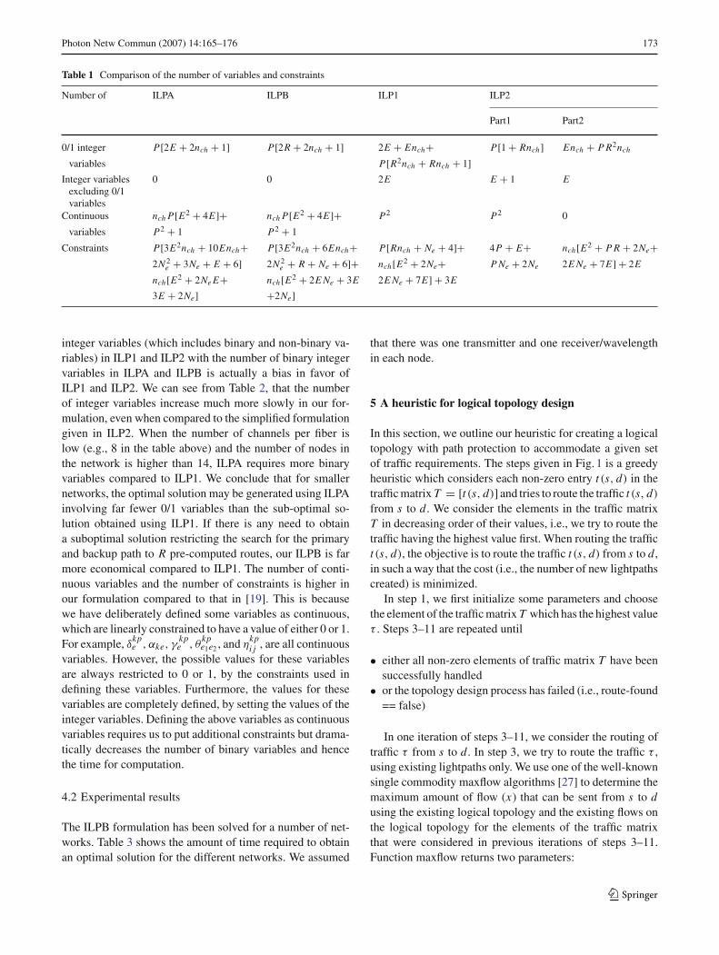
For our complexity analysis, we consider an arbitrary phy-sical network with Ne nodes, E edges, nch channels per fiber,and P = Ne × (Ne − 1) potential logical edges. We thendetermine the number of integer variables, continuous va-riables and constraints in our formulations (ILPA and ILPB)and compare these values to the corresponding values for theILP formulations (ILP1 and ILP2) given in [19]. We showthe results in Table 1. The most important factor affectingthe complexity of the ILP is the number of integer (binary)variables in the formulation [26], since the complexity in-creases exponentially with the number of binary variables.

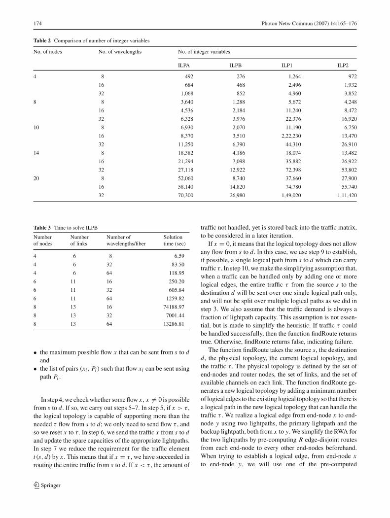
Table 2 illustrates how quickly the number of integervariables increase with the size of the network and the num-ber of available wavelengths per fiber. We note that ILP2,Part 1, always needs fewer binary variables than ILP2, Part2. For this reason, we have only shown the number of inte-ger variables needed in ILP2 part 2. For simplicity, we havecombined the non-binary integer variables in ILP1 and ILP2with the binary integer variables. Comparing the number of

123


Table 1 Comparison of the number of variables and constraints

Number of ILPA ILPB ILP1 ILP2

Part1 Part2

0/1 integer P[2E + 2nch + 1] P[2R + 2nch + 1] 2E + Ench+ P[1 + Rnch] Ench + P R2nch

variables P[R2nch + Rnch + 1]Integer variables

excluding 0/1variables

0 0 2E E + 1 E

Continuous nch P[E2 + 4E]+ nch P[E2 + 4E]+ P2 P2 0

variables P2 + 1 P2 + 1

Constraints P[3E2nch + 10Ench+ P[3E2nch + 6Ench+ P[Rnch + Ne + 4]+ 4P + E+ nch[E2 + P R + 2Ne+2N 2

e + 3Ne + E + 6] 2N 2e + R + Ne + 6]+ nch[E2 + 2Ne+ P Ne + 2Ne 2E Ne + 7E] + 2E

nch[E2 + 2Ne E+ nch[E2 + 2E Ne + 3E 2E Ne + 7E] + 3E

3E + 2Ne] +2Ne]

integer variables (which includes binary and non-binary va-riables) in ILP1 and ILP2 with the number of binary integervariables in ILPA and ILPB is actually a bias in favor ofILP1 and ILP2. We can see from Table 2, that the numberof integer variables increase much more slowly in our for-mulation, even when compared to the simplified formulationgiven in ILP2. When the number of channels per fiber islow (e.g., 8 in the table above) and the number of nodes inthe network is higher than 14, ILPA requires more binaryvariables compared to ILP1. We conclude that for smallernetworks, the optimal solution may be generated using ILPAinvolving far fewer 0/1 variables than the sub-optimal so-lution obtained using ILP1. If there is any need to obtaina suboptimal solution restricting the search for the primaryand backup path to R pre-computed routes, our ILPB is farmore economical compared to ILP1. The number of conti-nuous variables and the number of constraints is higher inour formulation compared to that in [19]. This is becausewe have deliberately defined some variables as continuous,which are linearly constrained to have a value of either 0 or 1.For example, δkp

e , αke, γkpe , θ

kpe1e2 , and η

kpi j , are all continuous

variables. However, the possible values for these variablesare always restricted to 0 or 1, by the constraints used indefining these variables. Furthermore, the values for thesevariables are completely defined, by setting the values of theinteger variables. Defining the above variables as continuousvariables requires us to put additional constraints but drama-tically decreases the number of binary variables and hencethe time for computation.

4.2 Experimental results

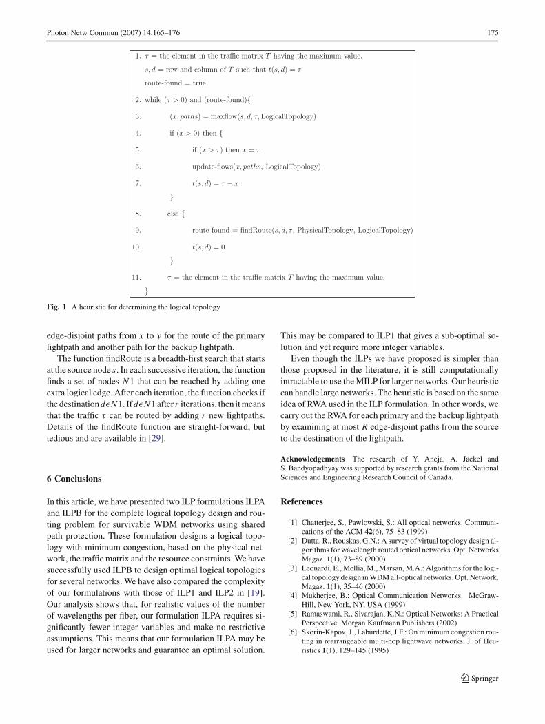
The ILPB formulation has been solved for a number of net-works. Table 3 shows the amount of time required to obtainan optimal solution for the different networks. We assumed

that there was one transmitter and one receiver/wavelengthin each node.

5 A heuristic for logical topology design

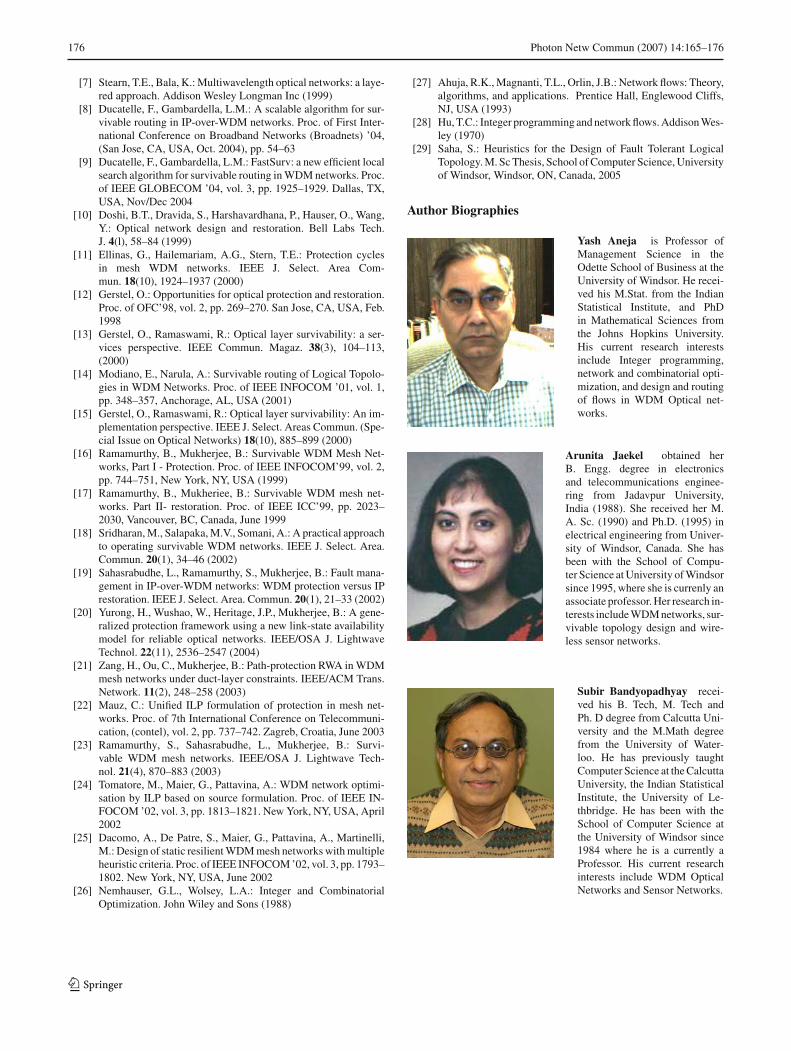
In this section, we outline our heuristic for creating a logicaltopology with path protection to accommodate a given setof traffic requirements. The steps given in Fig. 1 is a greedyheuristic which considers each non-zero entry t (s, d) in thetraffic matrix T = [t (s, d)] and tries to route the traffic t (s, d)

from s to d. We consider the elements in the traffic matrixT in decreasing order of their values, i.e., we try to route thetraffic having the highest value first. When routing the traffict (s, d), the objective is to route the traffic t (s, d) from s to d,in such a way that the cost (i.e., the number of new lightpathscreated) is minimized.

In step 1, we first initialize some parameters and choosethe element of the traffic matrix T which has the highest valueτ . Steps 3–11 are repeated until

• either all non-zero elements of traffic matrix T have beensuccessfully handled

• or the topology design process has failed (i.e., route-found== false)

In one iteration of steps 3–11, we consider the routing oftraffic τ from s to d. In step 3, we try to route the traffic τ ,using existing lightpaths only. We use one of the well-knownsingle commodity maxflow algorithms [27] to determine themaximum amount of flow (x) that can be sent from s to dusing the existing logical topology and the existing flows onthe logical topology for the elements of the traffic matrixthat were considered in previous iterations of steps 3–11.Function maxflow returns two parameters:

123


Table 2 Comparison of number of integer variables

No. of nodes No. of wavelengths No. of integer variables

ILPA ILPB ILP1 ILP2

4 8 492 276 1,264 972

16 684 468 2,496 1,932

32 1,068 852 4,960 3,852

8 8 3,640 1,288 5,672 4,248

16 4,536 2,184 11,240 8,472

32 6,328 3,976 22,376 16,920

10 8 6,930 2,070 11,190 6,750

16 8,370 3,510 2,22,230 13,470

32 11,250 6,390 44,310 26,910

14 8 18,382 4,186 18,074 13,482

16 21,294 7,098 35,882 26,922

32 27,118 12,922 72,398 53,802

20 8 52,060 8,740 37,660 27,900

16 58,140 14,820 74,780 55,740

32 70,300 26,980 1,49,020 1,11,420

Table 3 Time to solve ILPB

Number Number Number of Solutionof nodes of links wavelengths/fiber time (sec)

4 6 8 6.59

4 6 32 83.50

4 6 64 118.95

6 11 16 250.20

6 11 32 605.84

6 11 64 1259.82

8 13 16 74188.97

8 13 32 7001.44

8 13 64 13286.81

• the maximum possible flow x that can be sent from s to dand

• the list of pairs (xi , Pi ) such that flow xi can be sent usingpath Pi .

In step 4, we check whether some flow x, x �= 0 is possiblefrom s to d. If so, we carry out steps 5–7. In step 5, if x > τ ,the logical topology is capable of supporting more than theneeded τ flow from s to d; we only need to send flow τ , andso we reset x to τ . In step 6, we send the traffic x from s to dand update the spare capacities of the appropriate lightpaths.In step 7 we reduce the requirement for the traffic elementt (s, d) by x . This means that if x = τ , we have succeeded inrouting the entire traffic from s to d. If x < τ , the amount of

traffic not handled, yet is stored back into the traffic matrix,to be considered in a later iteration.

If x = 0, it means that the logical topology does not allowany flow from s to d. In this case, we use step 9 to establish,if possible, a single logical path from s to d which can carrytraffic τ . In step 10, we make the simplifying assumption that,when a traffic can be handled only by adding one or morelogical edges, the entire traffic τ from the source s to thedestination d will be sent over one single logical path only,and will not be split over multiple logical paths as we did instep 3. We also assume that the traffic demand is always afraction of lightpath capacity. This assumption is not essen-tial, but is made to simplify the heuristic. If traffic τ couldbe handled successfully, then the function findRoute returnstrue. Otherwise, findRoute returns false, indicating failure.

The function findRoute takes the source s, the destinationd, the physical topology, the current logical topology, andthe traffic τ . The physical topology is defined by the set ofend-nodes and router nodes, the set of links, and the set ofavailable channels on each link. The function findRoute ge-nerates a new logical topology by adding a minimum numberof logical edges to the existing logical topology so that there isa logical path in the new logical topology that can handle thetraffic τ . We realize a logical edge from end-node x to end-node y using two lightpaths, the primary lightpath and thebackup lightpath, both from x to y. We simplify the RWA forthe two lightpaths by pre-computing R edge-disjoint routesfrom each end-node to every other end-nodes beforehand.When trying to establish a logical edge, from end-node xto end-node y, we will use one of the pre-computed

123


Fig. 1 A heuristic for determining the logical topology

edge-disjoint paths from x to y for the route of the primarylightpath and another path for the backup lightpath.

The function findRoute is a breadth-first search that startsat the source node s. In each successive iteration, the functionfinds a set of nodes N1 that can be reached by adding oneextra logical edge. After each iteration, the function checks ifthe destination dεN1. If dεN1 after r iterations, then it meansthat the traffic τ can be routed by adding r new lightpaths.Details of the findRoute function are straight-forward, buttedious and are available in [29].

6 Conclusions

In this article, we have presented two ILP formulations ILPAand ILPB for the complete logical topology design and rou-ting problem for survivable WDM networks using sharedpath protection. These formulation designs a logical topo-logy with minimum congestion, based on the physical net-work, the traffic matrix and the resource constraints. We havesuccessfully used ILPB to design optimal logical topologiesfor several networks. We have also compared the complexityof our formulations with those of ILP1 and ILP2 in [19].Our analysis shows that, for realistic values of the numberof wavelengths per fiber, our formulation ILPA requires si-gnificantly fewer integer variables and make no restrictiveassumptions. This means that our formulation ILPA may beused for larger networks and guarantee an optimal solution.

This may be compared to ILP1 that gives a sub-optimal so-lution and yet require more integer variables.

Even though the ILPs we have proposed is simpler thanthose proposed in the literature, it is still computationallyintractable to use the MILP for larger networks. Our heuristiccan handle large networks. The heuristic is based on the sameidea of RWA used in the ILP formulation. In other words, wecarry out the RWA for each primary and the backup lightpathby examining at most R edge-disjoint paths from the sourceto the destination of the lightpath.

Acknowledgements The research of Y. Aneja, A. Jaekel andS. Bandyopadhyay was supported by research grants from the NationalSciences and Engineering Research Council of Canada.

References

[1] Chatterjee, S., Pawlowski, S.: All optical networks. Communi-cations of the ACM 42(6), 75–83 (1999)

[2] Dutta, R., Rouskas, G.N.: A survey of virtual topology design al-gorithms for wavelength routed optical networks. Opt. NetworksMagaz. 1(1), 73–89 (2000)

[3] Leonardi, E., Mellia, M., Marsan, M.A.: Algorithms for the logi-cal topology design in WDM all-optical networks. Opt. Network.Magaz. 1(1), 35–46 (2000)

[4] Mukherjee, B.: Optical Communication Networks. McGraw-Hill, New York, NY, USA (1999)

[5] Ramaswami, R., Sivarajan, K.N.: Optical Networks: A PracticalPerspective. Morgan Kaufmann Publishers (2002)

[6] Skorin-Kapov, J., Laburdette, J.F.: On minimum congestion rou-ting in rearrangeable multi-hop lightwave networks. J. of Heu-ristics 1(1), 129–145 (1995)

123


[7] Stearn, T.E., Bala, K.: Multiwavelength optical networks: a laye-red approach. Addison Wesley Longman Inc (1999)

[8] Ducatelle, F., Gambardella, L.M.: A scalable algorithm for sur-vivable routing in IP-over-WDM networks. Proc. of First Inter-national Conference on Broadband Networks (Broadnets) ’04,(San Jose, CA, USA, Oct. 2004), pp. 54–63

[9] Ducatelle, F., Gambardella, L.M.: FastSurv: a new efficient localsearch algorithm for survivable routing in WDM networks. Proc.of IEEE GLOBECOM ’04, vol. 3, pp. 1925–1929. Dallas, TX,USA, Nov/Dec 2004

[10] Doshi, B.T., Dravida, S., Harshavardhana, P., Hauser, O., Wang,Y.: Optical network design and restoration. Bell Labs Tech.J. 4(l), 58–84 (1999)

[11] Ellinas, G., Hailemariam, A.G., Stern, T.E.: Protection cyclesin mesh WDM networks. IEEE J. Select. Area Com-mun. 18(10), 1924–1937 (2000)

[12] Gerstel, O.: Opportunities for optical protection and restoration.Proc. of OFC’98, vol. 2, pp. 269–270. San Jose, CA, USA, Feb.1998

[13] Gerstel, O., Ramaswami, R.: Optical layer survivability: a ser-vices perspective. IEEE Commun. Magaz. 38(3), 104–113,(2000)

[14] Modiano, E., Narula, A.: Survivable routing of Logical Topolo-gies in WDM Networks. Proc. of IEEE INFOCOM ’01, vol. 1,pp. 348–357, Anchorage, AL, USA (2001)

[15] Gerstel, O., Ramaswami, R.: Optical layer survivability: An im-plementation perspective. IEEE J. Select. Areas Commun. (Spe-cial Issue on Optical Networks) 18(10), 885–899 (2000)

[16] Ramamurthy, B., Mukherjee, B.: Survivable WDM Mesh Net-works, Part I - Protection. Proc. of IEEE INFOCOM’99, vol. 2,pp. 744–751, New York, NY, USA (1999)

[17] Ramamurthy, B., Mukheriee, B.: Survivable WDM mesh net-works. Part II- restoration. Proc. of IEEE ICC’99, pp. 2023–2030, Vancouver, BC, Canada, June 1999

[18] Sridharan, M., Salapaka, M.V., Somani, A.: A practical approachto operating survivable WDM networks. IEEE J. Select. Area.Commun. 20(1), 34–46 (2002)

[19] Sahasrabudhe, L., Ramamurthy, S., Mukherjee, B.: Fault mana-gement in IP-over-WDM networks: WDM protection versus IPrestoration. IEEE J. Select. Area. Commun. 20(1), 21–33 (2002)

[20] Yurong, H., Wushao, W., Heritage, J.P., Mukherjee, B.: A gene-ralized protection framework using a new link-state availabilitymodel for reliable optical networks. IEEE/OSA J. LightwaveTechnol. 22(11), 2536–2547 (2004)

[21] Zang, H., Ou, C., Mukherjee, B.: Path-protection RWA in WDMmesh networks under duct-layer constraints. IEEE/ACM Trans.Network. 11(2), 248–258 (2003)

[22] Mauz, C.: Unified ILP formulation of protection in mesh net-works. Proc. of 7th International Conference on Telecommuni-cation, (contel), vol. 2, pp. 737–742. Zagreb, Croatia, June 2003

[23] Ramamurthy, S., Sahasrabudhe, L., Mukherjee, B.: Survi-vable WDM mesh networks. IEEE/OSA J. Lightwave Tech-nol. 21(4), 870–883 (2003)

[24] Tomatore, M., Maier, G., Pattavina, A.: WDM network optimi-sation by ILP based on source formulation. Proc. of IEEE IN-FOCOM ’02, vol. 3, pp. 1813–1821. New York, NY, USA, April2002

[25] Dacomo, A., De Patre, S., Maier, G., Pattavina, A., Martinelli,M.: Design of static resilient WDM mesh networks with multipleheuristic criteria. Proc. of IEEE INFOCOM ’02, vol. 3, pp. 1793–1802. New York, NY, USA, June 2002

[26] Nemhauser, G.L., Wolsey, L.A.: Integer and CombinatorialOptimization. John Wiley and Sons (1988)

[27] Ahuja, R.K., Magnanti, T.L., Orlin, J.B.: Network flows: Theory,algorithms, and applications. Prentice Hall, Englewood Cliffs,NJ, USA (1993)

[28] Hu, T.C.: Integer programming and network flows. Addison Wes-ley (1970)

[29] Saha, S.: Heuristics for the Design of Fault Tolerant LogicalTopology. M. Sc Thesis, School of Computer Science, Universityof Windsor, Windsor, ON, Canada, 2005

Author Biographies

Yash Aneja is Professor ofManagement Science in theOdette School of Business at theUniversity of Windsor. He recei-ved his M.Stat. from the IndianStatistical Institute, and PhDin Mathematical Sciences fromthe Johns Hopkins University.His current research interestsinclude Integer programming,network and combinatorial opti-mization, and design and routingof flows in WDM Optical net-works.

Arunita Jaekel obtained herB. Engg. degree in electronicsand telecommunications enginee-ring from Jadavpur University,India (1988). She received her M.A. Sc. (1990) and Ph.D. (1995) inelectrical engineering from Univer-sity of Windsor, Canada. She hasbeen with the School of Compu-ter Science at University of Windsorsince 1995, where she is currenly anassociate professor. Her research in-terests include WDM networks, sur-vivable topology design and wire-less sensor networks.

Subir Bandyopadhyay recei-ved his B. Tech, M. Tech andPh. D degree from Calcutta Uni-versity and the M.Math degreefrom the University of Water-loo. He has previously taughtComputer Science at the CalcuttaUniversity, the Indian StatisticalInstitute, the University of Le-thbridge. He has been with theSchool of Computer Science atthe University of Windsor since1984 where he is a currently aProfessor. His current researchinterests include WDM OpticalNetworks and Sensor Networks.

123

Documents

Some studies on path protection in WDM networks