Spatial change: continuity, reversibility, and emergent shapes

Spatial change: continuity, reversibility and emergent shapes

Ramesh Krishnamurti

Department of Architecture, Carnegie Mellon University, Pittsburgh, 15213, U.S.A

Rudi Stouffs

Architecture and CAAD, Swiss Federal Institute of Technology, Zurich, Switzerland

November 28, 1995 (revised) May 5, 1996

Abstract

Spatial composition can be viewed as computations involving spatial changes each

expressed as s − f(a) + f(b), where s is a shape, and f(a) is a representation of the emergent

part (shape) that is altered by replacing it with the shape f(b). We examine this formula in

three distinct but related ways. We begin by exploring the conditions under which a

sequence of spatial changes is continuous. We next consider the conditions under which

such changes are reversible. We conclude with the recognition of emergent shapes, i.e., the

determination of transformations f that make f(a) a part of s. We enumerate the cases for

shape recognition within algebras Uij, 0 ≤ i ≤ j ≤ 3 and within Cartesian products of these

algebras.

Spatial change

Computer-aided design is often nothing more than an euphemism for computer-aided

drafting, generally referring to systems that serve as repositories for designed information.

All too often newer approaches disguise old technology in new garments. (1) Design is

about change; design systems are formalisms which accommodate a notion of change;

computer-aided design is a process that employs computational mechanisms to effect

change. The manner of change affects the way the worlds of possible designs can be

(1) To some, taken literally, this statement is patently false when applied to disciplines where the foci

of interest center on the functional and behavioural descriptions associated with designed objects.

These descriptions are (typically, hierarchically) structured relationships between items of known

semantic types. In disciplines where design is through assembly, object-oriented approaches or case-

based design can be useful and effective. Where design proceeds by composition, where the objective

is not solely the designed object but also the discovery or manipulation of new ‘components’ along the

way, these methods, by their very nature, are ineffectual. It is this aspect of novelty which we believe

to be fundamental to design.

2 Shape Emergence: Spatial change

explored. A particularly enticing and related concept is that of emergence (Mitchell, 1993;

Stiny, 1993a, 1994).

New spatial objects and changes to spatial objects are produced by manipulative

operations on spatial objects. We consider a system for manipulating spatial objects. Such a

system [at least, implicitly] includes all objects that can be produced by the manipulative

operations, which at a minimum, comprise the spatial arithmetic operations and geometrical

transformations. Let s be an object (of interest) within this system. The basic operation of

producing a new shape (to the system) is by ‘adding’ to s in a specified manner, which we

can describe as s s + b. The symbol denotes a derivation of a new spatial object

from a given object. In this case, the new object is derived from the given object s by adding

the object b.

We may, of course, add the spatial object b, not as simply, but through some functional or

transformational form of it. Thus, s s + f(b), where f(b) is some transformation of the

object b.

Equally, a new object can be produced by ‘removing’ from s in some specified manner,

which we can describe as s s − f(a). We note here that the production of new spatial

objects by updating some aspects or properties of an existing object can be regarded as

‘addition’ or ‘subtraction’ depending on how the function f and the operators ‘+’ and ‘−’ are

defined.

We can, of course, effect change to s by the removal and subsequent addition of aspects or

properties of s by the formula s s − f(a) + g(b), where, in effect, f(a) is the altered part

and g(b) is its replacement. If we accept the possibility that ‘nothing’ can be added or

removed from s and still effect a change to s, the above formula is equivalent to two

changes, applied in sequence, each expressed as the formula

s s − f(a) + f(b),

where a or b may refer to an ‘empty’ object.

We can stipulate conditions on the application of this formula. For instance, if we impose

the condition that there be a connection between a and s − that is, there is a truth-functional

ψ such that s s − f(a) + f(b) can only be applied if ψ(s, f(a)) is satisfied − then we arrive

at the familiar notion of a ‘rule,’ a → b. Typically, ψ is satisfied when certain aspects or

properties of a ‘occur’ in s. If we impose the further condition that any and all changes are

Shape Emergence: Spatial change 3

effected only through formulae of this form, the system then specifies a ‘grammar.’ Of

particular importance is the notion of occurrence, for it is those emergent aspects or

properties of the object of interest that one normally wishes to change. The derivation s

s − f(a) + f(b) may be viewed as representing a basic equation of spatial change where f(a) is

a representation of the emergent properties in s that is being altered.

We claim that this formula captures nearly every kind of spatial editing change.

Consider, for example, the change s f(s) specifies a simple transformation of s. Here, the

emergent shape is, simply, s. In practice, we would replace s by f(s) directly rather than treat

it as an application of the rule s → f-(s), under an identity transformation.

The formula is interesting in two respects. Firstly, it offers a simple mechanism for

structuring change. Secondly, it specifies which aspects of s that we have to look for in

effecting the change. It is the latter that influences the way in which humans perceive

objects, and affects the way in which they perceive change. This perception is particularly

important to designers in their explorations of spatial forms.

In this paper, the objects are shapes and the changes are spatial changes. Functions on

shapes can be considered to be geometrical transformations. We can specify a part relation,

whereby any part of a shape is a shape. That is, a shape identifies an indefinite number of

shapes, each part of the original shape. Shapes emerge under the part relation – albeit –

these may not, originally, have been envisioned as such. Emergent shapes only become

explicit when manipulated as such. Recognizing emergent shapes requires determining a

transformation under which a shape is a part of the original shape.

The idea that designs are the products of evolving spatial changes has been considered by

others – for example, by Bridges (1991) who, informally, explores the [presumed] role of

computers in the design studio, and less informally by the Oxmans (1991), again in a

pedagogical context, who advocate that an understanding of precedents can be achieved

through analyses of spatial [transformational] change, which they refer to as refinement and

adaptation. The notion of studying spatial change – either informally or formally – is not

new. Figure 1 illustrates a design for a church by Leonardo da Vinci (from Leonardo Da

Vinci Engineer and Architect, The Montreal Museum of Fine Arts, 1987). This is an

example of many designs that Leonardo created with the irregular octagon, a form with

which he was fascinated. It is a cross-shaped radiating plan with alternating chapels and

niches. The satellite chapels connect diagonally converging into the central space. The

4 Shape Emergence: Spatial change

octagon dominates the plan. It is interesting to see how Leonardo used the unevenly spaced

grid and the [progressively added] axial lines to sculpt the emergent octagon [though he was

not always successful in this endeavour]. Figure 1 illustrates how an octagon emerges by

the superposition (or addition) of the two sets of grid lines.

The plan illustrates the three aspects of spatial change that form the subject matter of this

paper. Firstly, the development of the plan through spatial transformation (change) of the

underlying grid. Secondly, emergence of the octagons by delineating certain parts of the

grid and axial lines. Finally, there is an overall structure and continuity of composition.

Figure 1 Design of a church by Leonardo da Vinci (circa 1500).

Figure 2 Emerging octagon by adding two sets of grid lines

Shape Emergence: Shape rules and algebra 5

Shape rules and algebra

A shape rule is a mechanism that effects a spatial change. A shape rule a → b specifies a

spatial relationship between a and b, which when applied to a shape s under a transformation

f such that f(a) is a part of s, replaces f(a) in s by f(b) under rule application. That is, when

the shape rule is applied to the shape s it produces the shape, s f(a) + f(b). The set F of

valid transformations, commonly, is the set of all Euclidean transformations, which

comprise translations, rotations, reflections and scale.

A shape rule constitutes a formal specification of shape recognition and subsequent

manipulation. For a shape rule a → b, the left-hand side a specifies the similar shape to be

recognized, the right-hand side b specifies the replacement leading to the resulting shape. A

shape rule application consists of replacing the emergent shape corresponding to a, under

some allowable transformation, by b, under the same transformation.

Shape rules operate on shapes within an algebra, U, which is closed under the operations

of sum (shape union) ‘+’, difference ‘−’ and product (shape intersection) ‘⋅’, and a set of

transformations F. We define a part relation ‘≤’ on U such that f(a) ≤ s whenever a is a

shape in s for some member f of F.

Shapes form algebras under the part relation with well-defined properties (Stiny, 1991;

Stouffs, 1994). We denote a shape algebra by Uij, the set of all shapes made up of

i-dimensional elements embedded in a j-dimensional Euclidean space Ej, j ≥ i; by Ui if j is

understood; and by U, in general.

Shapes can be augmented in a number of ways, for instance, by distinguishing certain

parts of the shape, which introduce additional spatial relations. For instance, we can attach

labels from a given set to points. Labeled points, so formed, are ordered pairs that can be

arranged into sets to specify, in a manner analogous to U0, an algebra V0 of labeled points.

Spatial transformations of labeled points keep the labels the same though the points may

alter. Likewise, labels attached to the same point combine under sum. Thus, a labeled

shape can be considered as an element of the algebra V = U × V0. V has the same properties

as U. A labeled shape is made up of a shape and a finite, possibly empty, set of labeled

points. Other augmentations of shapes are possible (Stiny, 1992).

6 Shape Emergence: Shape description and topology

Shape description and topology

When designers work with shapes they do so in a manner quite distinct from the

(computational) representations for shapes. Often, this has to do with the process of

designing and with explanations for design choices or decisions. In other words, a shape is

structured so as to provide a description for it. Typically, this structuring takes the form of a

decomposition of the shape into parts, the sum of which equals the shape.

A particular form of a decomposition of a shape corresponds to a topology, which is

closed under sum and product (Hocking and Young, 1988). A topology for a shape satisfies

two additional conditions. Firstly, both the shape and the empty shape are in the topology.

Secondly, for any shape x which is a part of the given shape, there is a smallest shape in the

topology of which x is also a part. Every element of the topology is a part of the shape.

Thus, the sum of the elements of the topology equals the shape. A topology for a shape

specifies a way of cutting up a shape into a collection of fixed parts. A shape can have any

number of topologies defined on it.

There are two obvious topologies for a shape s, the trivial topology consisting of the

empty shape, 0, and the shape, s, and the infinite topology made up of all parts of s. The

more interesting topologies are those that cut up a shape somewhere in between these

extremes (Stiny, 1994). Figure 3 illustrates a shape and a topology defined on it.

Related to topologies for a shape are closure relations defined on shapes. A closure

relation c on a shape s is a mapping between parts of s that satisfies the following conditions.

i. c(0) = 0 and c(s) = s

ii. x ≤ c(x)

iii. c(c(x)) = c(x)

iv. c(x + y) = c(x) + c(y)

In addition, a closure relation c has the following properties.

v. x ≤ y ⇒ c(x) ≤ c(y)

vi. c(x ⋅ y) ≤ c(x) ⋅ c(y)

We denote the topology for a shape s by Ts, and its closure relation by cs. The connection

between a topology and its closure relation is strong in the sense that each specifies the

other. For any part x ≤ s, its closure cs(x) is an element of Ts. In fact, every element of Ts is

a closed shape. For shape s, with closure relation cs, .Ts cs x( )∪=

≤

Shape Emergence: Shape description and topology 7

New shapes can be produced from a shape by the application of shape rules. A shape rule

may be considered as a mapping between two shapes. Alternatively, as shown below, a

shape rule relates the descriptions (topologies) of the two shapes. A computation, from one

shape to another, is a series of shape rule applications that results in the production of the

second shape from the first.

Consider a shape s with topology Ts. Suppose the shape rule a → b is applicable to s.

Then, there is a transformation f such that f(a) ≤ s. Under shape rule application, we have,

t = s − f(a) + f(b).

There are two distinct ways in which such rule applications can be considered:

constructively and apperceptively. (2)

(2) ‘Doing’ and ‘seeing’ as George Stiny puts it. (Private communication)

Figure 3 A shape and a possible topology for it.

shape

topology

8 Shape Emergence: Shape description and topology

It is perhaps instructive to first examine the constructive effect of spatial change that is

wrought by rule application. We treat a rule as a function that ‘acts’ on parts of s. There are

a number of ways in which such a function can be expressed.

We note that t can be rewritten as:

t = s − f(a − b) + f(b − a).

That is, a → b has the same effect as the rule (a − b) → (b − a) where the left and right hand

shapes are now disjoint. However, f(b − a) may have parts in common with s. Thus:

t = s − f(a − b) + [f(b − a) − s].

Here, f(a − b) is a part of s, [f(b − a) − s] has no part in common with s, and the rule is

reduced to one in which the left and right hand shapes are disjoint, and the replacement

shape has no part in common with the given shape.

We can characterize this behavior of rule application by the function:

h(x) = if x ⋅ ≠ 0

= x otherwise, (1)

where = f(a − b) and = f(b − a) − s ≡ f(b) − s. Note that h affects those parts of s that

have something in common with f(a), but not in common with f(b). → provides a

representation of the shape rule a → b under the transformation f, , a representation of the

emergent shape, , a representation of the replacement shape, and h, a representation of the

application of the shape rule. The properties of h are given in table 1. The proof follows

directly from the definition of h.

It is important to note that although → has the same effect as a → b, these are not

equivalent rules either constructively and apperceptively. The rule → applies to more

spatial situations in s than does the rule a → b. Equally, it is important to note that → is

its own representation under the transformation f.

x = 0 h(0) = 0

x = s h(s) = t

x, y ≤ s

h(x + y) = h(x) + h(y)

h(x ⋅ y) ≤ h(x) ⋅ h(y)

x ≤ y ⇒ h(x) ≤ h(y)

Table 1 Properties of h

x a– b+ a

a b

a b

a

b

a b

a b

a b

Shape Emergence: Shape description and topology 9

h maps parts of s to parts of t, and, in the process, may be considered to induce a division

of t into a set of parts, Tt. For the closure relation cs on s, we can consider the relation ct:

ct(x) = h(cs(x ⋅ s)) + if x ⋅ ≠ 0

= h(cs(x)) otherwise.

Note that if x ⋅ = 0, x ≤ s. ct basically leaves untouched those closed shapes of s which

have no part in common with the replacement shape; otherwise, it adds to each closed

shape. ct satisfies the properties of a closure relation on t as proven below.

We note that ct(0) = h(cs(0)) = h(0) = 0.

We have ct(t) = h(cs(x ⋅ s)) + ≤ h(cs(s)) + = h(s) + = t. That is, ct(t) ≤ t.

If (x + y) ⋅ = 0, then ct(x + y) = h(cs(x + y)) = h(cs(x) + cs(y)) = h(cs(x)) + h(cs(y)) =

ct(x) + ct(y). Otherwise, ct(x + y) = h(cs((x + y) ⋅ s)) + = h(cs(x ⋅ s)) + h(cs(y ⋅ s)) + =

ct(x) + ct(y).

We now show that for x ≤ t, x ≤ ct(x). We note that x ⋅ = 0. If x ⋅ = 0, h(x) = x.

x ≤ cs(x) ⇒ h(x) ≤ h(cs(x)) ⇒ x ≤ ct(x). If x ≤ , then x ≤ h(cs(x ⋅ s)) + = ct(x). If neither

holds, then x can be partitioned with respect to , x = (x − ) + (x ⋅ ), and the inequality

naturally follows.

From ct(t) ≤ t and t ≤ ct(t), ct(t) = t, and ct( ) = h(cs( ⋅ s)) + = .

We have only ct(ct(x)) ≤ ct(x) left to consider. We have two cases to consider.

Suppose x ⋅ = 0. ct(x) = h(cs(x)). If cs(x) ⋅ = 0, ct(x) = cs(x), and ct(ct(x)) = ct(cs(x)) =

h(cs(cs(x))) = h(cs(x)) = ct(x). Otherwise, ct(x) = cs(x) − + . ct(ct(x)) = ct(cs(x) − ) +

ct( ) = h(cs(cs(x) − )) + ≤ h(cs(x)) + = cs(x) − + = ct(x).

If x ⋅ ≠ 0, ct(x) = h(cs(x ⋅ s)) + = cs(x ⋅ s) − + . ct(ct(x)) = ct(cs(x ⋅ s) − ) + ct( )

= h(cs(cs(x ⋅ s) − )) + ≤ h(cs(x ⋅ s)) + = cs(x ⋅ s) − + = ct(x).

Whence, the set is a topology for shape t.

b b

b

b

b b b

b

b b

a b

b b

b b b

b b b b

b a

a b a

b a b b a b

b b a b a b

a b b a b

Tt ct x( )

≤∪=

10 Shape Emergence: Rule application and continuity

Rule application and continuity

Stiny (1994) offers an interesting characterization of shape rule application that is related to

the way a shape is cut up into parts to form a description. In his paper, he gives a

handsomely deconstructivist interpretation whereby the present (shape) explains the

precedent (shape) which justifies the present, and does so through the concept of continuity.

We provide further elaboration.

Two topologies are related by a mapping that is deemed continuous whenever each closed

shape in one topology is mapped into a closed shape in the other (Stiny, 1994). We consider

the mapping h, defined previously, that relates two shapes s and t, and hence, their respective

topologies Ts and Tt. Formally, h is continuous whenever for x ≤ s, h(cs(x)) ≤ ct(h(x)), where

cs and ct are the closure relations in Ts and Tt. The continuity of h is now explored.

Consider any part x ≤ s. x ⋅ = 0. If x ⋅ = 0, h(x) = x, and ct(h(x)) = ct(x) = h(cs(x)).

Otherwise, consider a partitioning of x with respect to : x = x − + x ⋅ .

h(x) = x +

ct(h(x)) = ct(x − ) + ct( ) = h(cs(x − )) + h(cs( ))

h(cs(x)) = h(cs(x − ) + cs(x ⋅ )) = h(cs(x − )) + h(cs(x ⋅ )).

Whence,

h(cs(x)) ≤ ct(h(x))

⇔ h(cs(x − )) + h(cs(x ⋅ )) ≤ h(cs(x − ) + h(cs( ))

⇔ h(cs(x ⋅ )) ≤ h(cs(x − )) + h(cs( ))

⇔ cs(x ⋅ ) + ≤ cs(x − ) +

⇔ cs(x ⋅ ) ≤ cs(x − ) + (since cs(x ⋅ ) ⋅ = 0).

Since this must hold for any x ≤ s, it must also hold for x = ⇒ cs( ) = . Furthermore,

for x ≤ s, cs(x ⋅ ) ≤ cs( ), 0 ≤ cs(x − ), and thus, cs(x ⋅ ) ≤ cs( ) = ≤ cs(x − ) + .

It follows that cs( ) = is a necessary and sufficient condition for the rule application to

be continuous. That is, the representation of the emergent shape has to be closed in the

topology of s.

However, this condition is dependent on the specific choice of the function h. For

different choices for h, different conditions exist for the rule application to be continuous.

For instance, if we choose h as:

b a

a a a

a b

a b a b

a a a a

a a a b

a a b

a a b a a b

a a a a b

a a a

a a a a a a a a

a a

Shape Emergence: Rule application and continuity 11

h(x) = [x + cs(f(b) ⋅ s)]− f(a) + f(b) if x ⋅ f(a) ≠ 0

= x otherwise, (2)

and ct as:

ct(x) = h[cs(x ⋅ s) + cs(f(b) ⋅ s)] + f(b) if x ⋅ (f(b) − s) ≠ 0

= h(cs(x)) otherwise,

we can show that h (as defined by (2)) satisfies the properties in table 1, and that ct specifies

the closure relation for a topology for t. It is important to note that the term cs(f(b) ⋅ s) is

required to account for all parts of the replacement shape f(b) that has parts in common with

s. In this case, we can show, following an argument similar to the one above, that cs(f(a)) ≤

f(a) + cs(f(b) ⋅ s) is a necessary and sufficient condition for the rule application to be

continuous. Here, the condition for continuity of shape rule application is also independent

of x, but dependent on s, f(a) and f(b), as well as the topology defined on s by the closure

relation cs. There are two cases to consider with respect to this condition.

There are a set of rules for which rule application is always continuous, regardless of the

topology defined. These are strictly additive rules, for which a ≤ b, or cs(f(a)) ≤ cs(f(b) ⋅ s).

Note that this is equivalent to the condition, = 0.

Any rule application may be considered continuous if we choose the topology for s

carefully so that cs(f(a)) ≤ cs(f(b) ⋅ s) + f(a). We can examine this condition more closely for

its effect and condition on a topology.

Suppose we partition f(a) with respect to cs(f(b) ⋅ s). We then have,

cs(f(a)) = cs(f(a) − cs(f(b) ⋅ s)) + cs(f(a) ⋅ cs(f(b) ⋅ s)).

The second term is always a part of cs(f(b) ⋅ s); thus, we can rewrite the condition as:

cs(f(a) cs(f(b) ⋅ s)) ≤ f(a) + cs(f(b) ⋅ s).

Given the properties of the closure operation, we can restate this condition upon the

elements of the topology as follows: there exists a closed shape y of the topology Ts, such

that

f(a) − cs(f(b) ⋅ s) ≤ y ≤ f(a) + cs(f(b) ⋅ s)

If a ≤ b, then f(a) − cs(f(b) ⋅ s) = 0, and y = 0 becomes a solution. Since the empty shape 0 is

always an element in the topology Ts, additive rules are always continuous, as we saw

before.

We note that y = f(a − b) = constitutes a solution.

a

a


If f(b) ⋅ s = 0, there is exactly one solution, namely, y = f(a). Notice that this is similar to

the situation previously considered; here, = f(a) and = f(b).

Table 2 gives the continuity conditions on h as defined by (2). In general, the specific

range of solutions depends on the closure relation, as we need to evaluate cs(f(b) ⋅ s).

Discussion

Stiny demonstrates the relationship between continuity and shape emergence in the

following way. Every shape rule computation can be made continuous provided one can

structure topologies [and hence, descriptions] for shapes so that emergent shapes are

distinguished in the descriptions. He offers a construction in which every topology in the

sequence representing a series of shape rule applications contains as an element the

emergent shape that is altered by the corresponding shape rule in the sequence. It should be

noted that the sequence of topologies is induced retroactively.

Stiny develops his formulation in order to give an account of emergence in shape

computation. As a consequence, he requires that the emergent shapes are distinguished as

such in descriptions of shapes. For a shape rule a → b, f(a) is generally considered the

emergent shape, but any shape that is a part of f(a + b) ⋅ s and has f(a b) as a part, can be

considered a representation of the emergent shape. Thus, a representation of the emergent

shape has to be closed in each topology in the series that defines a computation for it to be

continuous. As the analysis above indicates this requirement is strong. In other words,

continuity of computation requires anticipation of the emergent shapes that are to be

changed.

h(x) = [x + cs(f(b) ⋅ s)]− f(a) + f(b) if x ⋅ f(a) ≠ 0

= x otherwise

a ≤ b

f(a) ∈ Ts

y ∈ Ts

f(a) − cs(f(b) ⋅ s)) ≤ y ≤ f(a) + cs(f(b) ⋅ s))f(a − b) ∈ Ts

f(a + b) ⋅ s ∈ Ts

Table 2 Continuity of h.

a b

Shape Emergence: Rule application and continuity 13

This proposition complements Stiny’s original result. Although every shape rule

computation can be made continuous, retroactive induction illustrates only the potential for

continuity; for computations to be continuous, representations of the emergent shapes have

to be closed (and thus, anticipated either way) in the descriptions within a computation.

It is important to note that the solution f(a) ∈ Ts is independent of b, but it is not

independent of cs, namely, the way in which a shape is decomposed into its description.

The solution f(a) ∈ Ts is a continuity condition for all shape rules of the form a → k. In fact,

in this case, it is the only solution. Notice that this condition does not presuppose any

conditions on the replacement shape and s.

The solution f(a) ∈ Ts is most interesting, and unarguably, the most intuitive. It is also the

condition that best draws out the apperceptive nature of shape rule application. Consider the

spatial change under an application of the rule a → a. In fact, s does not change. Yet,

sequences of spatial changes that include rules of the form a → a will not be continuous

unless f(a) ∈ Ts. That is, in order to ensure continuity of computation, in general,

descriptions of s have to be altered even when no spatial change has occurred. The shape

rule a → a may be viewed as reflecting the situation where designers pause and

‘contemplate’ the design hitherto. The mere act of observing one’s design might have the

effect of changing its description. This remark – as it pertains to the act of designing – gets

into the realms of philosophy and cognitive psychology, in neither areas of which would we

consider ourselves competent. See, for example, Stiny (1995).

One can, of course, impose an arbitrary topology on shapes where the emergent shape is

always an element, and restrict shape rule application to known elements. This then ensures

that for each such ‘object-oriented’ view of a shape, computations involving known objects

(within that view) will be continuous. However, these will also be independent of

precedent. If, as Stiny shows, one wants ‘interesting’ computations that distinguish

emergent shapes, then these, by necessity, involve precedent and are only object-oriented

after the fact. (3)

The above result is not altogether surprising for spatial computations involving object-

oriented descriptions. Taking any standard textbook definition of objects, it is straight-

forward to identify an isomorphism between objects and an augmented algebra of shapes

made up of ‘point’ figures, A0 ⊆ U0 × A, where the elements of U0 are indices to the objects.

A, of course, may reflect spatial and non-spatial attributes. Computation is, essentially,


defined on finite sets of points. Technical difficulties, if any, lie in the manner in which

elements of A can be operated on, for example, the inheritance of attributes or properties.

For spatial computations to be interesting, notions of emergence have to be introduced into

the definition and treatment of objects.

It is possible to ensure continuous computations by always distinguishing the emergent

shape f(a). In certain situations this will be possible by restructuring the topologies prior to

each shape rule application, and always if this restructuring is carried out retroactively

following Stiny’s procedure.

The restructuring of descriptions opens up interesting issues in design thinking. For

example, if we accept the hypothesis that descriptions convey structure and meaning – in

other words, the topology sits within a system of features such as hierarchical classification

schemes, for example, semantic networks or objected-oriented systems made up of known

components with known semantics – and given that all spatial changes can be effected by

mechanisms of the form given by s s − f(a) + f(b), the preceding analysis suggests that

there is a distinction to be drawn between descriptions that designers use while designing

and descriptions that designers employ to explain their designs. This may explain the

‘discrepancy’ that often surfaces between the avowed process, as evidenced by their stated

descriptions and reasons, that designers claim to adopt at the start of their design and the

actual process, again as evidenced by their stated descriptions and reasons, that they follow

in arriving at their designs. If we accept that continuity of descriptions is a measure of

articulate consistency, this may explain why object-oriented approaches and case-based

(3) The inherent dynamism of descriptions is a property that does not solely belong to the realm of

design. There are striking parallels in other areas that demonstrate the connection between continuity,

precedent and emergence. Stiny cites sources in law where one seeks articulate consistency or, at the

very least, continuity from precedent in order to explain a current legal position. In genetics,

hereditary diseases such as cystic fibrosis or sickle-cell anaemia have been linked to certain DNA

patterns within genes – researchers have attempted to establish historical precedents for present-day

patterns that can be explained through evolutionary gene mutation – in doing so, they have, sometimes,

reclassified or redefined their taxonomies The historian, Edward Hallett Carr, makes the same point in

the traditional field of historical research. In his book, What is History, Carr (1961, pp 35, 164)

declares history to be “… a continuous process of interaction between the historian and his facts, an

unending … dialogue between the events of the past and the progressively emerging future ends. The

historian’s interpretation of the past, his selection of significant and the relevant, evolves with the

progressive emergence of new goals” [our italics]. It seems that valid classifications, which can

‘explain’ designs, are equally post-rationalised.

Shape Emergence: Reversible and irreversible rules 15

reasoning are becoming increasingly popular in computer-aided design precisely because

operations on such descriptions are continuous. However, the analysis shows these systems

will be bereft of novelty, where novelty arises in situations where the designer does not view

a spatial entity as a fixed object with fixed descriptions, but perceives it to be malleable, and

thus can be reshaped thereby producing new spatial (and consequently, new semantic)

relationships. It is these emergent shapes made up of parts from known objects that, we

believe, contribute to novelty in design.

Reversible and irreversible rules

Rules combine to form grammars which are formal rewriting systems for producing objects

of interest. A shape grammar combines a set of shape rules. A shape grammar defines a

language, the set containing all shapes, generated by the grammar, that have no associated

symbols. Figure 4 shows a few shapes produced from an initial shape using just a single

rule. All shapes produced are members of the language of the corresponding grammar.

Computationally, an important issue is whether one can easily backtrack along a

computation to a shape from which alternative spatial forms may be explored. Related to

this is the question: whether for any rule in a grammar, a reverse rule can be constructed that,

when applying, consecutively, the original and the reverse rule to any element of the algebra

Figure 4 Exemplar derivations from an initial shape with a single rule.

⇒

rule:

→

derivations:

⇒ ⇒ ⇒

⇒ ⇒⇒

⇒

16 Shape Emergence: Reversible and irreversible rules

over which the grammar is defined, the result is identical to the original element. If it is the

case that the rules are all reversible, the corresponding grammar is said to be reversible.

The ability to reverse spatial computations is important for systems in which one can

explore design spaces. If computations are reversible, then a simple recording of the

changes that have been hitherto invoked is all that is required to return to any previous state.

If computations are not reversible, additional shape information has to be recorded. The

question then is whether the price of additional book-keeping may be offset by the greater

flexibility that irreversible rules offer to exploring the world of possible designs.

We now consider the reversibility of shape rule application.

Consider a shape rule a → b that applies to a shape s. Then,

t = s − f(a) + f(b) = s − f(a − b) + f(b − a) = s − f(a − b) + [f(b − a) − s].

Assume that there is a rule x → y, which may be identical to b → a, such that the shape

that results from applying to s, the rules a → b and x → y in that order and under the same

transformation f, equals s. We can assume that the rule x → y applies under the same

transformation; otherwise, we can always transform the rule such that it applies under the

same transformation, without changing the rule application or its scope. Thus,

s = t − f(x) + f(y) = t − f(x − y) + f(y − x) = t − f(x − y) + [f(y − x) − t].

Whence:

s = (s − f(a − b) + [f(b − a) − s]) − f(x − y) + [f(y − x) − t]

= s − f(a − b) − f(x − y) + [f(b − a) − s − f(x − y)] + [f(y − x) − t]

Since f(x − y) ⋅ s = 0 and [f(b − a) − s] ⋅ s = 0, the above equation implies the following:

f(b − a) − s − f(x − y) = 0 and s = s − f(a − b) + [f(y − x) − t].

Thus, f(b − a) − s ≤ f(x − y) and f(a − b) ≤ f(y − x) − t.

Similarly, substituting the expression for s in the expression for t, we obtain:

f(x − y) ≤ f(b − a) − s and f(y − x) − t ≤ f(a − b).

Therefore, f(x − y) = f(b − a) − s and f(y − x) − t = f(a − b).

These two equations give a specification for x and y in terms of the rule a → b, as well as

the shape s under application. The rule x → y is independent of s only if f(b − a) ⋅ s = 0 so

that f(x − y) = f(b − a). Similarly, note that a → b is the reverse rule for x → y for all shapes

t only when f(y − x) ⋅ t = 0. This condition was first given in Krishnamurti (1981) though not

formally proved there.

Shape Emergence: Reversible and irreversible rules 17

Discussion

Irreversibility of shape rules distinguishes shape grammars from most other grammar

formalisms. Intuitively, we note that when combining two shapes (or sets) under the

operation of ‘+’, identical elements ‘merge’. That is, only a single occurrence of the element

appears in the resulting shape or set. In the case of set grammars, if u denotes the

cardinality of a set u, max( u , v ) ≤ u + v ≤ u + v . On the other hand, in the case of

string or graph grammars (given an appropriate definition for the size of a graph) this would

constitute strict equality. No comparable measure exists for shapes except for shapes

defined in U0.

The condition f(b − a) ⋅ s = 0 is an expression of this situation. f(b − a) denotes the shape

that is added to s, which is not previously removed, under rule application. If the product

with s equals zero, no elements merge, and the rule application is reversible. The condition

is, generally, dependent on the particular rule application, i.e., on the original shape s and

transformation f. In the case that b ≤ a, f(b − a) = 0 and thus the rule is reversible

independent of the shape to which (and the transformation under which) it is applied. These

constitute purely subtractive rules. It is interesting to note that if a → b is a reversible rule,

its reverse rule b → a is not unless b = a.

Figures 5 and 6 respectively illustrate a reversible and an irreversible shape rule. In

general, shape rules are irreversible. Yet, every shape rule computation can be reversed

provided one records the mergent shape f(b − a) ⋅ s for each rule application in the

computation such that these shapes can be added, appropriately, in a reversal of

computation. In other words – unlike most spatial computational systems – it does not

suffice to merely record the acts of change, but also requires recording a representation of

the spatial changes along with the acts. Thus, like continuity, reversibility of computation

requires anticipation. In this case it requires an anticipation of the mergent shape f(b − a) ⋅ s

within the original shape s.

The significance from a design standpoint, to us, at any rate, stems from the fact that

designing is a temporal activity. The irreversibility of a rule has the effect of time stamping

each rule application and, thus, capturing design ‘intent’ at any given time.

It should be noted that whenever a reversible rule a → b is applied in a computation,

shape b does not add to the description (topology) of the resulting shape. It should be further

noted that the application of the reverse rule b → a at a subsequent stage in the computation

18 Shape Emergence: Reversible and irreversible rules

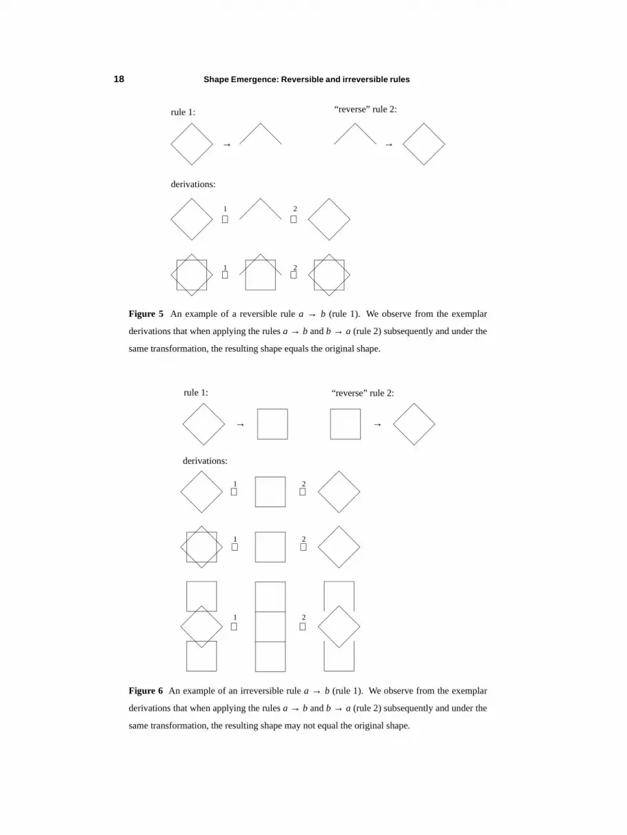
Figure 5 An example of a reversible rule a → b (rule 1). We observe from the exemplar

derivations that when applying the rules a → b and b → a (rule 2) subsequently and under the

same transformation, the resulting shape equals the original shape.

⇒ ⇒

“reverse” rule 2:rule 1:

→

derivations:

1 2

→

⇒ ⇒1 2

Figure 6 An example of an irreversible rule a → b (rule 1). We observe from the exemplar

derivations that when applying the rules a → b and b → a (rule 2) subsequently and under the

same transformation, the resulting shape may not equal the original shape.

⇒ ⇒1 2

⇒ ⇒

⇒ ⇒

“reverse” rule 2:rule 1:

→ →

derivations:

1 2

1 2

Shape Emergence: Shape recognition 19

under the same transformation f removes any trace of the effect of the original application on

the design. However, in the case of an irreversible rule a → b, the application of the rule

b → a under the same transformation f does not remove the effect of the original rule

application on the design. Moreover, for reversible rules, the computation to produce a

given design may be indifferent to the ordering of rule applications. This is because the

parts of the shape that are affected by the rules remain the same. This is not the case with

irreversible rules. Thus, general shape rule application is both spatial and temporal.

Shape recognition

We have thus far examined two distinct aspects of the application of a shape rule a → b to a

shape s. In our analyses we have assumed the existence of an affine transformation f such

that f(a) ≤ s. We now turn our attention to the question of determining all f’s that satisfy the

subshape relation, f(a) ≤ s. In general, shape recognition relates to finding one or all valid

transformations under which a shape is a part of a given shape. In the case of shape rule

application the solution to this problem consists of finding a correspondence between the

spatial elements in the left hand side of the rule, a, and elements of the given shape, s, and

determining the transformation f that represents this correspondence. (4) This is a hard

problem because a shape, with definite description, has indefinitely many ‘touchable’ parts.

In respect to this problem, we take the position that shapes are individuals as reflected by the

part relation defined on shapes. (5)

We consider shape recognition in each shape algebra, and across shape algebras (table 3).

Shape recognition in U0 is equivalent to set recognition and is thus trivial. For shapes in U1,

distinguishable points serve as the basis for reducing the problem (Krishnamurti, 1981;

(4) Some readers may be familiar with the equivalent problem in set or graph grammars, respectively

termed subset and subgraph detection, that consists of searching for either a single entity or a group of

entities within a set or a graph. Such a search is straightforward; it requires a one-to-one matching of

entities that are identical under a certain transformation. The determination of the matching is not

necessarily efficient, for example, subgraph isomorphism is NP-complete. On the other hand, a

prerequisite for shape rule computation is that any subshape of a shape is spatially replaceable.

(5) The concept of individuals differs from the generally accepted concept of classes (or sets) in that

no subdivision into subclasses or members is established or suggested a priori (Leonard and

Goodman, 1940). Stiny (1993b), in a reversal of his earlier position (Stiny, 1982), offers a comparison

between shapes and individuals, which differ algebraically. However, both shapes and individuals can

be divided into parts in any way whatsoever.

https://www.researchgate.net/publication/23541867_Shapes_are_individuals?el=1_x_8&enrichId=rgreq-7f3581db-9a91-4e24-8da5-903747c78cb1&enrichSource=Y292ZXJQYWdlOzIzNTQxMDI2O0FTOjEwMjAyNTcyNzU3ODEyMkAxNDAxMzM2MjM4MzQz

20 Shape Emergence: Shape recognition

Chase, 1989; Krishnamurti and Earl, 1992). For any given shape, its distinguishable points

correspond to points (labeled or otherwise) the properties of which (with respect to the

shape) are preserved under the part relation and affine transformations. Points of

intersection of segments in a shape are distinguished. The application of this concept to Ui,

for i > 0, is explored below.

In Uii, all shapes are necessarily co-equal. Consequently, no distinguishable points, lines

or planes can be constructed. As a result, for i > 0, an indeterminate number of transforma-

tions exist, the base transformation of which is the identity transformation. In U00, only the

identity transformations exists.

In j dimensions, a correspondence between j+1, not co-hyperplanar, distinguishable

points uniquely determines an affine transformation. However, for determining all valid

similarity transformations, j such points suffice, provided the corresponding ‘point figures’

are similar to each another. Each such transformation remains subject to evaluation with

respect to the shape a. Otherwise, if j, co-hyperplanar distinguishable points cannot be

determined, then there may be an indeterminate number of valid transformations. In such

cases, one can isolate a set of base transformations from which the other transformations can

be generated. Figure 7 illustrates this indeterminacy of transformations for shapes in U23

(see case 2.2 below).

In the sequel, we restrict discussion to similarity transformations. Note that even in the

case of shapes with rational descriptions, the resulting transformations may not be rational

(Krishnamurti and Earl, 1992). As such, the constructions described below do not guarantee

exact arithmetic.

U0 U00 U01 U02 U03 …

U1 U11 U12 U13 …

U2 U22 U23 …

U2 U33 …

Table 3 Table of shape algebras.

https://www.researchgate.net/publication/23540658_Shapes_and_shape_grammars_From_mathematical_model_to_computer_implementation?el=1_x_8&enrichId=rgreq-7f3581db-9a91-4e24-8da5-903747c78cb1&enrichSource=Y292ZXJQYWdlOzIzNTQxMDI2O0FTOjEwMjAyNTcyNzU3ODEyMkAxNDAxMzM2MjM4MzQz

https://www.researchgate.net/publication/23540782_Shape_Recognition_in_Three_Dimensions?el=1_x_8&enrichId=rgreq-7f3581db-9a91-4e24-8da5-903747c78cb1&enrichSource=Y292ZXJQYWdlOzIzNTQxMDI2O0FTOjEwMjAyNTcyNzU3ODEyMkAxNDAxMzM2MjM4MzQz

https://www.researchgate.net/publication/23540782_Shape_Recognition_in_Three_Dimensions?el=1_x_8&enrichId=rgreq-7f3581db-9a91-4e24-8da5-903747c78cb1&enrichSource=Y292ZXJQYWdlOzIzNTQxMDI2O0FTOjEwMjAyNTcyNzU3ODEyMkAxNDAxMzM2MjM4MzQz

Shape Emergence: Detecting emergent shapes in Ui 3 21

Detecting emergent shapes in Ui 3

We give the determinate and indeterminate cases for shapes defined on Ui 3, i < 3. Since the

representation of a shape in Ui 3 is embedded in E3, we distinguish the cases in E3 using as

primary distinguishable elements the distinct carriers of the segments in the shape to be

recognized. Additional distinguishable points may be constructed for the purpose of

generating a determinate number of valid transformations, though the cases themselves are

identified by the primary distinguishable elements. The cases are grouped by their shape

algebra and numbered accordingly: the first digit denotes the dimensionality of the algebra.

In the sequel, a denotes the shape to be recognized in the given shape s.

The cases for U03

The cases are trivial. There is one determinate case when at least three non-colinear

(distinguishable) points in the given shapes can be found. Otherwise, a possible

indeterminate number of valid transformations between the shapes exist.

Case 0.1 There are three non-colinear points.

Three non-colinear points uniquely determine an affine transformation in E2, i.e., for the

plane these define. In E3, if the ‘point figures’ are similar, this results in two Euclidean

transformations, of which one can be derived from the other using a reflection in this plane.

Figure 7 The base transformation maps carriers onto carriers without scaling: (a) no possible

transformation exists, even under scaling; (b) an infinite number of possible transformations

exist under scaling.

subshape:

(a)

(b)

22 Shape Emergence: Detecting emergent shapes in Ui 3

A fourth, non-coplanar, point suffices to invalidate one of these transformations.

Krishnamurti and Earl (1992) describe the computation of both transformations.

Case 0.2 There are two (distinct) points.

An indeterminate number of valid transformations exist. Given a base transformation

that maps both points in the shape to be recognized onto the respective points in the given

shape, the full set of possible transformations is derived using rotations about the line

connecting both points and a reflection in a plane through this line.

Case 0.3 There is a single point.

An indeterminate number of valid transformations exist. These can be derived from a

base transformation using (three-axes) rotations about this point, scalings that leave the

point fixed and a reflection in a plane through this point.

The cases for U13

The cases are completely described in Krishnamurti and Earl (1992). There are two

determinate cases, which are illustrated in Figure 8.

Case 1.1 There are two skew lines.

Skew lines are not parallel, nor do these intersect in a point. The common perpendicular

of two skew lines defines two distinguishable points, i.e., the feet of this perpendicular on

the lines. Since two points are sufficient to determine a fixed scaling factor, an additional

(distinguishable) point may be constructed on one of the lines. As such, this problem

reduces to Case 0.1, with three distinguishable points, for which a determinate number of

possible valid transformations exist. Krishnamurti and Earl (1992) describe a variant to this

construction.

Figure 8 Examples illustrating the determinate cases for U13:

(a) Case 1.1 and (b, c) Case 1.2.

(a) (b) (c)


Case 1.2 There are three coplanar lines, not all parallel, and not all concurrent at a

single point.

If no two lines are parallel, then, the intersection points of these lines constitute three

distinguishable points. Otherwise, the two points of intersection constitute two

distinguishable points that can be augmented with a third point constructed similar to Case

1.1.

There are also three indeterminate cases as illustrated in Figure 9.

Case 1.3 There are two non-parallel lines.

From a base transformation, all other transformations result from scalings that leave the

point of intersection fixed and a reflection in the plane defined by both lines.

Case 1.4 There are two (parallel) lines.

The full set of transformations is generated by composing a base transformation with

translations along the direction of the lines together with a reflection in a plane

perpendicular to the parallel lines.

Case 1.5 There is a single line.

The full set of possible transformations is found by composing the base transformation

with rotations about the line, denoted as l, scalings that leave a point on l fixed, translations

along the direction of l, and a reflection in a plane normal to l.

Figure 9 Examples illustrating the indeterminate cases for U13:

(a) Case 1.3, (b) Case 1.4 and (c) Case 1.5.

(a) (b) (c)

24 Shape Emergence: Detecting emergent shapes in Ui 3

The cases for U23

Krishnamurti and Stouffs (1993) identify the following cases. There is a single determinate

case, illustrated in Figure 10.

Case 2.1 There are four planes, not all parallel, and not all lines of intersection are

parallel, concurrent or coincident.

We can find two skew lines of intersection and reduce the problem to Case 1.1

consequently, for which there exists a determinate number of valid transformations.

There are five indeterminate cases in U23, illustrated in Figure 11.

Figure 10 Examples illustrating the determinate Case 2.1 for U23.

Figure 11 Examples illustrating the indeterminate cases for U23:

(a) Case 2.2, (b, c) Case 2.3, (d) Case 2.4, (e) Case 2.5 and (f) Case 2.6.

(d) (f)(e)

(b) (c)(a)


Case 2.2 There are three planes, and not all the lines of intersection are parallel or

coincident.

Another way to formulate this is the following: There are three planes, and their normal

vectors are linearly independent. All the lines of intersection are concurrent at a single

point, and the problem reduces to Case 1.3, for which there exists a possible indeterminate

number of valid transformations (under scaling and reflection).

Case 2.3 There are three planes, and these do not intersect in a single line.

All the lines of intersection may be parallel, but these do not coincide. This problem

reduces to Case 1.4, for which there exists a possible indeterminate number of valid

transformations (under translation and reflection).

Case 2.4 There are two non-parallel planes.

The full set of transformations is generated by composing a base transformation with

translations along the direction of the line of intersection together with scalings that leave a

point on this line fixed and a reflection in a perpendicular plane.

Case 2.5 There are two (parallel) planes.

A base transformation maps the carriers of the two planes in a onto the respective carriers

of two planes in s. All other transformations result from translations along two

perpendicular axes parallel to these planes, rotations about a line normal to both planes and a

reflection in a plane through this line.

Case 2.6 There is a single plane.

A base transformation maps the carrier of a plane in a onto the carrier of a plane in s. The

full set of possible transformations is generated by composing this base transformation with

translations along two perpendicular axes parallel to the plane, scalings that leave a point on

the plane fixed, rotations about a line normal to the plane and a reflection in a plane through

this line.

26 Shape Emergence: Shape recognition revisited

Shape recognition revisited

The preceding analysis considers all possible cases for each of the algebras Ui 3, 0 ≤ i ≤ 3.

However, in many cases, shape rule application is defined in a cartesian product of

algebra’s. Earlier we defined shape rule application in an algebra V = U × V0 of labeled

shapes. More generally, shape rule application can be defined in any cartesian product of

algebras U1 × U2 × …. As such, it is insufficient to enumerate the cases for each of the

algebras Ui 3 separately. Below, we consider the enumeration of the cases for any cartesian

product of algebras Ui 3, 0 ≤ i ≤ 3.

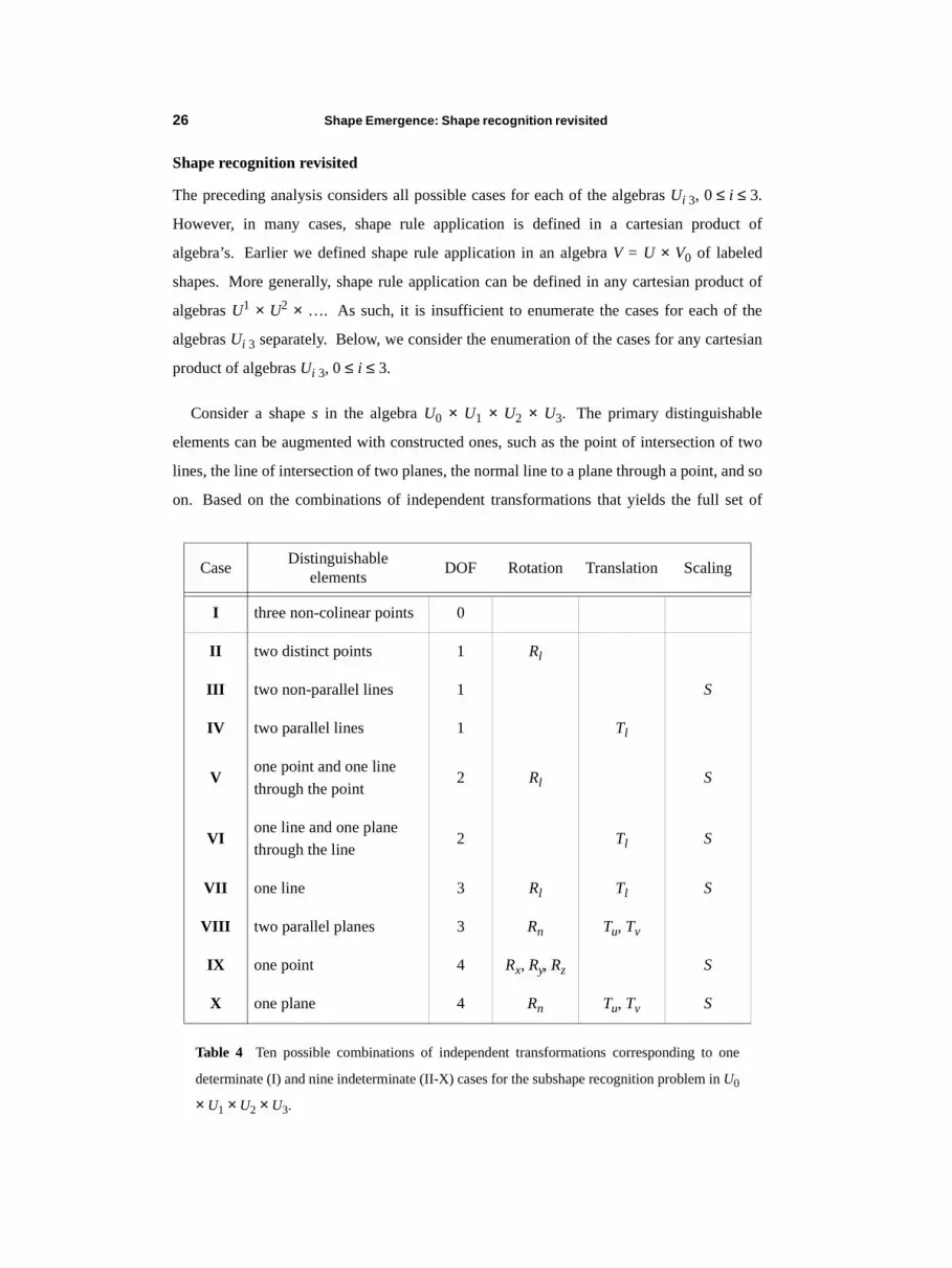
Consider a shape s in the algebra U0 × U1 × U2 × U3. The primary distinguishable

elements can be augmented with constructed ones, such as the point of intersection of two

lines, the line of intersection of two planes, the normal line to a plane through a point, and so

on. Based on the combinations of independent transformations that yields the full set of

Table 4 Ten possible combinations of independent transformations corresponding to one

determinate (I) and nine indeterminate (II-X) cases for the subshape recognition problem in U0

× U1 × U2 × U3.

CaseDistinguishable

elementsDOF Rotation Translation Scaling

I three non-colinear points 0

II two distinct points 1 Rl

III two non-parallel lines 1 S

IV two parallel lines 1 Tl

V one point and one line

through the point2 Rl S

VI one line and one plane

through the line2 Tl S

VII one line 3 Rl Tl S

VIII two parallel planes 3 Rn Tu, Tv

IX one point 4 Rx, Ry, Rz S

X one plane 4 Rn Tu, Tv S

Shape Emergence: Shape recognition revisited 27

possible valid transformations from a base transformation, only ten primary cases remain, of

which one represents the determinate case and the remaining nine the indeterminate cases.

We consider the degrees of freedom (DOF) corresponding to an indeterminate case to be the

number of independent transformations as such (not including a possible reflection). Single

transformations include a rotation about a line, a translation along a line and a scaling. A

single plane defines two independent translations; a general rotation about a single point

constitutes three independent rotations. We use T to denote a translation, with Tl a

translation along a line l and Tu and Tv two (perpendicular) translations parallel to a plane.

We use R to denote a rotation, with Rl a rotation about a line l, Rn a rotation about the normal

n to a plane and Rx, Ry and Rz rotations about the major axes. We use S to denote a scaling.

Table 5 All non-redundant cases with at least one distinguishable point, based on combina-

tions of primary distinguishable elements.

Distinguishable elementsCase DOF

Points Lines Planes

3 non-colinear I.a 0

2 1 non-perpendicular I.b 0

2 II.a 1

1 1 non-colinear I.c 0

1 1 colinear 1non-coplanar •

non-perpendicularI.d 0

1 1 colinear 1 coplanar III.a 1

1 1 colinear V.a 2

1 2non-colinear

intersectionI.e 1

1 2colinear

intersectionIII.b 1

1 1 non-coplanar II.b 1

1 1 coplanar V.b 2

1 IX.a 4


The ten determinate and indeterminate cases are summarized in Table 4. Cases II through

IV correspond to a single DOF, either rotational, translational or scaling. Cases V and VI

have two DOF of which one corresponds to a scaling necessarily, the other is either

rotational or translational. Cases VII and VIII have three degrees of freedom: a single

distinguishable line results in a translational DOF along the line, a rotational DOF about the

line, as well as a scaling; two parallel planes give way to a single rotational DOF and two

translational DOF. Cases IX and X have a maximal four degrees of freedom: either three

rotational or one rotational and two translational, together with a scaling. No other

Table 6 All non-redundant cases without distinguishable points but at least one distinguish-

able line, based on combinations of primary distinguishable elements.

Distinguishable elementsCase DOF

Lines Planes

3coplanar • not all parallel

• non-concurrentI.f 0

2 skew I.g 0

2 coplanar • non-parallel 1 non-concurrent I.h 0

2 coplanar • non-parallel III.c 1

2 parallel 1 non-parallel I.i 0

2 parallel IV.a 1

1 2

non-concurrent • not both

parallel or perpendicular

to line

I.j 0

1 2 perpendicular to line II.c 1

1 1non-parallel •

non-perpendiclarIII.d 1

1 1 parallel IV.b 1

1 1 perpendicular V.c 2

1 1 coplanar VI.a 2

1 VII.a 3


combinations are possible: an axis of rotation corresponds to a single DOF, a center of

rotation to three DOF, no construct allows for only two rotational DOF. Similarly, any

distinguishable element removes at least one translational DOF; only a distinguishable plane

allows for two translational DOF, but only a single rotational DOF.

Each primary case defines a set of secondary cases, each of which can be reduced to the

primary case by constructing additional distinguishable elements. However, it is

computationally expensive to construct all possible distinguishable elements a priori, in

order to determine the particular primary case. Therefore, we list below the secondary cases

for each primary case, for all possible cases of combinations of primary distinguishable

elements. Table 5 summarizes all non-redundant (6) cases with at least one distinguishable

point. Table 6 summarizes all non-redundant cases without distinguishable points but at

least one distinguishable line. Table 7 summarizes all cases with only distinguishable

planes, these correspond to the cases for U23. The cases enumerated below are numbered

according to their primary case. Thus, case d.n refers to the n-th secondary case for the d-th

primary case.

(6) An example of redundancy would be two distinguishable points and one line non-colinear with at

least one point: the second, possibly colinear, point is redundant as Case I.c shows.

Table 7 All non-redundant cases with only distinguishable planes

Distinguishable Planes Case DOF

4not all parallel •

not all intersection lines parallel or concurrentI.k 0

3 not all intersection lines parallel III.e 1

3 not concurrent in a single line IV.c 1

2 non-parallel VI.b 2

2 parallel VIII.a 3

1 X.a 4


Case I.a is identical to Case 0.1; it applies towards Case 1.1, Case 1.2 and Case 2.1 as

well. Case I.a represents primary case I.

Case I.a There are three non-colinear points.

We reduce each of the following cases to Case I.a by constructing the necessary

distinguishable points.

Case I.b There are two points together with a plane not perpendicular to the line

defined by both points.

If at least one point is not coincident with the plane, then construct the foot of the

perpendicular from this point onto the plane as a third distinguishable point. These three

points are not colinear, otherwise the plane would be perpendicular to the line through both

points. If both points are coincident with the plane, then construct a point on the normal

with the plane through one point, such that the distance to this point is identical to the

distance between the two original points (Figure 12).

Case I.c There is a point and a line not colinear with the point.

Construct the foot of the perpendicular from the point onto the line and construct a third

point on the line at equal distance from the foot as the distance between the foot and the first

point as shown in Figure 13(a) (Krishnamurti and Earl, 1992).

Case I.d There is a point, a line colinear with the point, and a plane neither

coincident with the point nor perpendicular to the line.

Construct the foot of the perpendicular from the point onto the plane. Since this point is

Figure 12 Illustrations to Case I.b: (a) at least one point not coincident with the plane and

(b) both points coincident with the plane.

p1

p2p3

p3

p2

p1p3’

(a) (b)


not colinear with the line, we have a situation similar to Case I.c. However, we can

construct a third point on the line at an equal distance from the original point as the distance

from the foot to this point. See Figure 13(b)).

Case I.e There is a point together with two planes which are not both coincident with

the point.

Since the line of intersection is not colinear with the point, this problem is reduced to

Case I.c.

Case I.f There are three coplanar lines, not all parallel, and not all concurrent at a

single point.

See Case 1.2.

Case I.g There are two skewed lines.

See Case 1.1.

Case I.h There are two coplanar non-parallel lines together with a plane, which are

not all concurrent at a single point.

Consider the point of intersection of both lines together with one of the lines, that is not

perpendicular to the plane, and the plane; this corresponds to Case I.d.

Case I.i There are two (parallel) lines and a plane which is neither parallel to the

lines nor coincident with a line.

Figure 13 Illustrations to (a) Case I.c and (b) Case I.d.

p1p2

p2

p3

p1

p2p3’

(a) (b)

p3’


Construct the intersection points of both lines with the plane. Construct a third point on

one of the lines at equal distance from the point of intersection of this line with the plane as

the distance between both intersection points (Figure 14(a)).

Case I.j There is a single line together with two planes, not both parallel or

perpendicular to the line, such that these are not all concurrent at a single point.

The construction is dependent on whether one of the planes is parallel to the line, or not.

If one plane is parallel to, but not coincident with, the line while the other plane is neither

parallel to, nor coincident with, the line, then, the line of intersection of both planes is skew

with respect to the original line (Figure 14(b)). This reduces to Case I.g or Case 1.1.

Otherwise, neither plane is parallel to, nor coincident with, the line, while not both planes

are perpendicular to the line and all three elements are not concurrent at a single point.

Consider the (two) points of intersection of the line with both planes together with the foot

of the perpendicular from one of the intersection points onto the other plane. These three

points cannot be colinear (Figure 15).

Case I.k There are four planes, not all parallel, and not all lines of intersection are

parallel, concurrent or coincident.

See Case 2.1.

Case II.a specifies a single axis of rotation (without scaling); it is identical to Case 0.2. It

represents primary case II.

Case II.a There are two (distinct) points.

Figure 14 Illustrations to (a) Case I.i and (b) Case I.j.

p1

p2

p3

p2

p1p3’

(a) (b)


We reduce each of the following cases to Case II.a by constructing the necessary

distinguishable points.

Case II.b There is one point, and one plane not coplanar with the point.

Construct the foot of the perpendicular from the point onto the plane. The resulting axis

of rotation (defined by both points) is perpendicular to the plane, such that the plane is

mapped onto itself under the transformation.

Case II.c There is one line, and two planes perpendicular to the line.

The two points of intersection of the line with the planes are distinct.

Cases III.a through III.e specify a scaling. Case III.c is the representative case; it is

identical to Case 1.3 and applies also to Case 2.2. We reduce each of the following cases to

Case III.c by constructing the necessary distinguishable lines.

Case III.a There is one point, one line and one plane, all coincident.

Construct a second line perpendicular to the first line, coincident with both the point and

the plane.

Case III.b There is a point, and two planes coincident with the point.

Construct the foot of the perpendicular from the point onto the plane. The resulting axis

of rotation (defined by both points) is perpendicular to the plane, such that the plane is

mapped onto itself under the transformation.

Figure 15 Illustrations to Case I.j.

p1

p2

p3

p3

p2

p1

p3’

(a) (b)

p3’


Case III.c There are two non-parallel lines.

See Case 1.3.

Case III.d There is one line and one plane; these are neither parallel nor

perpendicular.

Construct the line of intersection of a second plane coincident with the line and

perpendicular to the first plane with the first plane.

Case III.e There are three planes, and not all the lines of intersection are parallel or

coincident.

See Case 2.2.

Case IV.a specifies a single direction of translation (without scaling); it is identical to

Case 1.4 and applies also towards Case 2.3. Case IV.a represents primary case IV.

Case IV.a There are two parallel lines.

We reduce each of the following cases to Case IV.a by constructing the necessary

distinguishable lines.

Case IV.b There is one line and one parallel plane.

There exists a unique second line coincident with the plane and parallel to the first line,

such that the foot of the perpendicular from any point on the first line lies on the second line

(i.e., the second line constitutes a normal projection of the first line onto the plane).

Case IV.c There are three planes, and these do not intersect in a single line.

See Case 2.3.

Case V.a, which represents primary case V, specifies a single axis of rotation with scaling.

Case V.a There is a single point, and a line coincident with the point.

The line constitutes the axis of rotation, the single point inhibits any translation but allows

for a scaling (Krishnamurti and Earl, 1992). We reduce each of the following cases to Case

V.a by constructing the necessary distinguishable line and/or point.

Case V.b There is a single point, and a plane coincident with the point.

The normal line to the plane and coincident with the point constitutes the axis of rotation.


Case V.c There is a single line, and a plane perpendicular to the line.

The line constitutes the axis of rotation, the point of intersection of the line and plane

constitutes the fixed point.

Case VI.a, which represents primary case VI, specifies a single direction of translation

with scaling.

Case VI.a There is a single line, and a plane coincident with the line.

The line defines the direction of translation, the plane inhibits any rotation about the line

but allows for scaling.

Case VI.b There are two non-parallel planes.

See Case 2.4.

There is only one case, Case VII.a, which specifies a single axis of rotation, a single

direction of translation and a scaling. It is identical to Case 1.5.

Case VII.a There is a single line.

There is only one representative case, Case VIII.a, which specifies a single axis of

rotation and two (perpendicular) directions of translation (without scaling); it is identical to

Case 2.5.

Case VIII.a There are two (parallel) planes.

Case IX.a (the representative of primary case IX) specifies three (perpendicular) axes of

rotation and a scaling; it is identical to Case 0.3.

Case IX.a There is a single point.

Case X.a (the representative of primary case X) specifies a single axis of rotation, two

(perpendicular) directions of translation and a scaling; it is identical to Case 2.6.

Case X.a There is a single plane.

This completes the enumeration of the secondary cases.

Shape Emergence: Variations on a common theme 36

Variations on a common theme

The classification, according to the number and type of degrees of freedom, is based solely

on distinguishable elements. That is, only the carriers of the shape segments and not the

segments themselves define the specific classification. Each class is characterized by a base

transformation, from which all possible transformations can be derived in correspondence to

the DOF of this class. A possible transformation is a transformation that maps the given

shapes under the part relation. As such, the part relation defines a constraint on the possible

transformations.

Gero and Yan (1993, 1994) consider a notion of emergent shapes that are visually

recognized as such, which they refer to as emergent visual shapes. In particular, using

shapes in U1, they consider as an emergent visual shape, any shape that is embedded in the

carriers of the given shape and the segments of which are bounded by the points of

intersection of the carriers. (7) These carriers and their points of intersection precisely define

the distinguishable elements used to determine the class of transformations under shape

recognition. The resulting set of possible transformations is constrained by the embedding

of the segments of the transformed shape in the carriers (instead of the segments) of the

given shape.

Emergent shapes may be constrained by, say, topological, geometrical or dimensional

considerations. For instance, Gero and Yan require emergent visual shapes to be simple

closed polygons. A simple variant of the subshape recognition algorithm (Krishnamurti,

1981) can detect general emergent visual shapes. Stiny (1977, 1980) characterizes shape

recognition as dependent on a set of parameters specified on the emergent shape, together

with any constraints or bounds on the parameters. Other requirements include emergent

shapes augmented with attributes such as labels or weights. The enumeration of the

recognition cases for labeled (and weighted) shapes can proceed along the lines described in

this paper.

Acknowledgement

We would like to thank George Stiny for his helpful comments.

(7) Gero and Yan refer to the carriers of a given shape as infinite maximal lines. The concept of a

‘carrier’ expresses independence of dimensionality and generalizes emergent visual shapes to shapes

that are bounded by lines (or planes, volumes, etc.) of intersections of the carriers.

Shape Emergence: References 37

References

Bridges A H, 1991. “DAC or Design and Computers,” in G. Schmitt (ed.) CAAD

Futures’91, Vieweg, Weisbaden, 65−76

Carr E H, 1961. What is History? Vintage Books, New York.

Chase S C, 1989. “Shapes and shape grammars: from mathematical model to computer

implementation,” Environment and Planning B: Planning and Design, 16, 215−242

Gero J S and Min Yan, 1993. “Discovering Emergent Shapes Using a Data-Driven Symbolic

Model,” in U. Flemming and S. Van Wyk (eds.) CAAD Futures’93, Elsevier Science,

Amsterdam, 1−17

Gero J S and Min Yan, 1994. “Shape emergence by symbolic reasoning,” Environment and

Planning B: Planning and Design, 21, 191−212

Hocking J G and Young G S, 1988. Topology. Dover Publication, New York.

Krishnamurti R, 1981. “The construction of shapes,” Environment and Planning B:

Planning and Design, 8, 5−40

Krishnamurti R and Earl C F, 1992. “Shape recognition in three dimensions,” Environment

and Planning B: Planning and Design, 19, 585−603

Krishnamurti R and Stouffs R, 1993. “Shape Grammars: Motivation, Comparison and New

Results,” in U. Flemming and S. Van Wyk (eds.) CAAD Futures’93, Elsevier Science,

Amsterdam, 57−74

Leonard H S and Goodman N, 1940. “The Calculus of Individuals and Its uses,” The

Journal of Symbolic Logic 5, 45−55

Mitchell W M, 1993. “A Computational View of Design Creativity,” in J. S. Gero and M. L.

Maher (eds.) Modeling Creativity and Knowledge-Based Creative Design, Lawrence

Erlbaum Associates, Hillsdale, New Jersey, 25−42

Oxman R E and Oxman R M, 1991. “Refinement and Adaptation: Two Paradigms in Form

Generation in CAAD,” in G. Schmitt (ed.) CAAD Futures’91, Vieweg, Weisbaden, 313−

328

Stiny G, 1977. “Ice-ray: a note on Chinese lattice designs,” Environment and Planning B:


Stiny G, 1980. “Introduction to shape and shape grammars,” Environment and Planning B:


Stiny G, 1982. “Shapes are individuals,” Environment and Planning B: Planning and

Design 9, 359−367

Shape Emergence: References 38

Stiny G, 1991. “The Algebra of Designs,” Research in Engineering Design 2, 171−181

Stiny G, 1992. “Weights,” Environment and Planning B: Planning and Design 19, 413−430

Stiny G, 1993a. “Emergence and Continuity in Shape Grammars,” in U. Flemming and S.

Van Wyk (eds.) CAAD Futures’93, Elsevier Science, Amsterdam, 1993, 37−54

Stiny G, 1993b. “Boolean Algebra for Shapes and Individuals,” Environment and Planning

B: Planning and Design 20, 359−362

Stiny G, 1994. “Shape rules: closure, continuity and emergence,” Environment and Planning

B: Planning and Design 21, no. 7, s49–s78.

Stiny G, 1995. “Useless rules,” manuscript, Department of Design, University of California,

Los Angeles.

Stouffs R, 1994. The Algebra of Shapes. Ph.D. Dissertation, Department of Architecture,

Carnegie Mellon University, April 1994.

Documents

Spatial change: continuity, reversibility, and emergent shapes