Spatial Competition with Endogenous LocationChoices: An Application to Discount Retailing1

Ting Zhu Vishal Singh

April 2007

1The authors are Assistant Professor of Marketing at the Graduate School of Business,University of Chicago and Assistant Professor of Marketing respectively at Tepper School ofBusiness, Carnegie Mellon University. The paper is based on Ting Zhu’s thesis at CarnegieMellon University. The authors can be reached at vsingh@andrew.cmu.edu (Singh) andtzhu@chicagogsb.edu (Zhu) for comments and suggestions.

Abstract

This paper examines the importance of geographical differentiation in store location deci-sions of firms in the retail discount industry. Using a novel data set that includes the storelocations and accompanying market conditions for all stores belonging to the Wal-Mart,Kmart, and Target chains, we study the factors that influence the entry and location de-cisions of those firms. The model involves an incomplete information game between thethree players where each firm has private information about its own profitability. A keyfeature of our modeling approach is that it permits asymmetries across firms in the im-pact of exogenous market characteristics and competitive interaction effects. In addition,the variations in the exogenous firm specific characteristics, such as the distances fromthe market to firms’ headquarters and the distances to the nearest distribution centersprovide the source for model identification. Results show the importance of accountingfor firm asymmetries in their response to market conditions and competition interactions.We use the parameter estimates of the payoff functions to predict the equilibrium marketstructure under a variety of market conditions that provide additional insights into thecompetitive structure of the industry.

Keywords: Entry, discrete games, location choice, retail competition, discount stores

1 Introduction

Firms employ a variety of strategies to differentiate their product offerings from compe-

tition. In the retailing sector, these strategies include the breadth and depth of product

assortment, price, promotions, merchandise quality, customer service, and so forth. How-

ever, as a well known aphorism states, the three most important decisions in retailing

are location, location, and location. Indeed, store location has long been regarded as

a primary driver of retail competition and one of the most important factor in a con-

sumer’s store choice decision (Huff 1964, Arnold, Oum, and Tigert 1983, Brown 1989,

Craig et. al. 1989). Store location decisions are particularly important since they are less

adjustable in the short-run without incurring significant costs. On the other hand, other

marketing mix elements such as price and product assortment can readily be modified in

response to competition or other changes in the market. When deciding whether to enter

a particular local market and where to locate within that market, firms consider a variety

of factors including demand and cost conditions, logistical issues, and proximity to and

size of their consumer base. In addition, firms must account for the actual and potential

presence of competitors. While favorable market conditions such as large population base

and low cost labor encourage entry, such markets are also likely to attract competitors.

In the long-run, the interaction of these different factors determines the observed entry

patterns by firms.

In this paper, we study the strategic entry and location choice decisions in the retail

discount industry. For all practical purposes, the industry involves an oligopoly comprised

of three dominant firms: Wal-Mart, Kmart, and Target. Using a novel data set that

includes store locations and associated market conditions for all stores belonging to these

three chains, we study the factors that determine firm’s entry and location choices. We

partition the United States into a series of small markets and further divide each market

into a finite number of spatially distinct retail locations that are heterogeneous in demand

and cost conditions. We model the entry decisions as the outcome of an incomplete

information game between the three players where we assume that each firm has private

information about its own profitability, but only observes the distribution of its rivals’

profitability. In this game of location choices, distance to rivals serves as a form of

product differentiation. The empirical analysis then relates the predictions of the model

to observed behavior of the three chains. The resulting estimates provide insights into

the importance of numerous factors for store profitability. Most important, the analysis

provides insights into a fundamental tension faced by these firms, namely the desire to be

1

in attractive locations while also obtaining insulation from competition through spatial

differentiation.

Our modeling approach builds on the literature on static game theoretic models where

agents make discrete choices such as entry and exit decisions1. This literature endogenizes

the competitive structure in a market such as number of firms by implicitly analyzing

the first stage of a two-stage game in which firms first decide whether or not to enter

followed by price or quantity competition. The general premise is that the observed entry

decisions of firms and the associated industry structure in a market reveal information

about the underlying economic profits. The key insight that the analyst can infer features

of these profits even without information of price, quantity, or margins, since firms will

enter a market if and only if they expect positive profits. Unlike the structural models

of supply and demand that provide marginal conditions for optimal actions, the discrete

nature of entry and exit decisions implies threshold conditions for players’ unobserved

profits in order for a particular outcome to obtain. As such, the empirical approach to

analyze discrete games is intuitively analogous to that of single-agent discrete decision

processes in which estimation of underlying payoffs is based on inequality restrictions

that are required for a certain choice to be optimal. For example, in the marketing

literature, researchers have inferred parameters of utility functions through application

of this revealed preference argument to data on discrete choices by consumers. In both

the single-agent setting and the multi-agent game, the underlying objective is the same,

namely the estimation of unobserved latent payoffs using observed behavior. However,

whereas the single-agent problem involves an arguably independent decision, the inter-

dependencies in payoffs of agents in a game theoretic setting necessitates the use of

some equilibrium concept, most commonly Nash equilibrium or some refinement of Nash

equilibrium.

Bresnahan and Reiss (1987, 1990, 1991) and Berry (1992) provide early salvo into this

literature. They describe the general structure of such games and discuss some issues

that arise in empirical analysis of the model. One common problem endemic to models of

discrete strategic interaction is the presence of multiple equilibria in which certain values

of the underlying latent payoffs could simultaneously be consistent with more than one

1Obviously a more comprehensive model would explicitly consider dynamic entry patterns of firms.However, as noted by Reiss and Wolak (2006) in their recent review of the literature, “while someprogress has been made in formulating and solving such (dynamic) games, to date their computationaldemands have largely made them impractical for empirical work. As a consequence, almost all structuralmarket structure models are static”. In this paper we follow the literature on static entry games but (asnoted below) explicitly allow for firm heterogeneity.

2

equilibrium outcome. The presence of multiple equilibria complicates estimation since

the model does not provide exact probabilities for each outcome as would be required in

maximum likelihood estimation.2 This difficulty contrasts with the single-agent setting in

which the inequalities of the model provide a direct mapping from each possible value of

the latent payoffs to one, and only one, outcome. Two common solutions to the multiple

equilibria problem are to focus only outcomes that are common across all equilibria or

to change the structure of the game. An example of the first approach would involve

examining the total number of firms rather than their identities while the latter approach

could involve a sequential entry structure rather than a simultaneous move game. Mazzeo

(2002) extends this literature by incorporating product differentiation where a firm’s

payoff asymmetrically depends on whether a competitor is more or less similar to the

firm. However, in Mazzeo’s framework firms are restricted to choose from a few possible

product “types” as a larger choice set becomes computationally cumbersome due to the

large number of profit constraints that need to be satisfied in equilibrium. Seim (2001,

2005) solves this dimensionality problem by allowing firms to possess private information

about their own profitability. Her incomplete information approach circumvents the need

for checking a large number of entry configurations to find the equilibria and allows for a

considerably larger dimensional set of product types than is feasible in games of complete

information.

In this paper, we follow Seim (2001, 2005) by setting up the model as an incomplete

information game where players privately observe their own location-specific potential

profits, but observe only the distribution of their rivals’ profitability. Unlike previous

applications in the literature, we explicitly allow for asymmetries related to the identity

of the firms. The previous literature has assumed that firms are symmetric in terms of

their sensitivity to exogenous market conditions and in their impact on other competitors.

In other words, a firm’s profits depend on the total number of other firms in the market

rather than their actual identities beyond simple type differences as in Mazzeo (2002).

In reality, firms care about the actual identities of their competitors rather than simply

the total number of competitors3. For instance, entry by firms such as Exxon-Mobil,

Microsoft, Home Depot, or Citigroup into a geographical or product market may be

viewed by competing firms as a greater threat to profits than entry by smaller independent

2An additional complication is the complex inequalities that the model yields for a certain outcometo be an equilibrium. In terms of the stochastic structure of the model, these inequalities translate intocomplex regions of integration for the unobservables of the model. Berry (1992) introduced simulationtechniques in the context of entry games to deal with these issues.

3Kyle (2005) makes similar arguments in the context of entry in pharmaceutical drugs.

3

firms. In the current context of discount stores, such asymmetries may be crucial. For

instance, Kmart’s profit may be different when it faces a Wal-Mart rather than a Target

or when it faces a Wal-Mart supercenter rather than a Wal-Mart discount store. Similarly,

the impact of market demand and cost conditions may vary across firms as well as store

formats. As such, it is paramount to allow such asymmetries in an analysis of this

industry.

Our modeling approach allows for both competitive effects and preferences over ex-

ogenous market conditions to be firm-specific. A firm’s payoff from entering a market

and choosing a particular location depends on its expectation of the optimal location

choice of competitors, exogenous market characteristics that are common to all firms,

and other observed factors that are specific to each firm. Examples of common factors

include demand and cost conditions in the market such as population and retail wages,

while firm-specific factors could include variables related to logistical issues such as the

distance from a firm’s distribution center. In addition to the observed variables, all

firms’ profits also depend on market components that are unobserved by the analyst, but

are observed by all firms. For example, positive or negative marketwide shocks such as

availability of commercial land or restrictiveness of zoning laws are difficult to measure

and quantify, but are likely to play an important role in the entry decisions of all firms.

Finally, a firm’s payoff in each location includes a component specific to that firm and

location which could represent idiosyncratic operational costs or managerial talent that

are unobserved by both the analyst and other players.

The incomplete information model provides a tractable framework for studying the

complex interactions of optimal site selection in which a trade-off exists between prox-

imity to competitors and the desirability of certain location characteristics. The model

translates the discrete actions of competitors into smooth location choice probabilities

that represent the likelihood of competitor entry into a location rather than actual real-

izations, thus allowing for a larger set of locations (or product types) than is generally

feasible in games of complete information. The resulting Bayesian Nash equilibrium

(BNE) is derived using a nested fixed-point algorithm which is then embedded in a sim-

ulated maximum likelihood procedure to estimate the model parameters.

To implement the model, we assembled an original data set that includes all store

locations for the three largest players in the discount store industry: Wal-Mart, Kmart,

and Target. Interestingly, all three chains started in 1962 when Wal-Mart opened its first

store in Rogers, Arkansas, Kmart began operations in Garden City, Michigan, and Target

opened a store in Roseville, Minnesota. Over the next few decades, these firms expanded

4

their operations both domestically and internationally to reach dominant positions in

the retailing world. In the process, they have also experimented with several other retail

formats, most prominently the supercenter which involves a combination of a full-service

grocery store and a general merchandize outlet. The data includes the exact location

(latitude/longitude) of all stores in operation as of 2003 across the United States. We

partition the United States into a series of smaller markets and further divide each market

into smaller neighborhoods. Each store can then be mapped to one of these neighborhood

locations. Besides location, we observe certain other store characteristics such as format

and store size. In addition, we collected information on the location of both the firm’s

headquarters and its distribution centers. Distances from the distribution centers to

each market location are used as proxies to capture logistical issues in firm’s location

choice decisions. Finally, we supplement the data with detailed information collected

from the US Census Bureau and the Bureau of Labor Statistics to capture demand and

cost conditions at every geographical location.

In the empirical application, we create discrete distance bands around each location

to capture the effects of competitors and market size. The results show that population

in closer distance bands to a location contribute more to profitability than population

in distant bands. Interestingly, the parameters for distant population are significantly

larger for Wal-Mart, especially for its supercenter format, suggesting that Wal-Mart’s

trading area is larger than those of its rivals. All firms are found to prefer markets

with lower retail wages, markets where a larger proportion of families have children and

vehicles, and markets that are closer to their respective headquarters. We also find

significant differences across firms in certain demand characteristics. For instance, Wal-

Mart Supercenters are found to prefer markets with lower income levels, while Target

prefers markets with higher income and education levels. These results seem consistent

with common perceptions of these stores. For example, Target has been known to position

itself as an upscale discounter that caters to a higher income and better educated clientele

than its competitors. Similarly, lower income levels in Wal-Mart locations are consistent

with Wal-Mart’s everyday low pricing and value positioning. We also find that Wal-Mart,

particularly for its supercenter format, gives more weight to locations that are closer to

its distribution center, reflecting its logistical efficiencies.

In terms of competitive interactions, we find that proximity to competitors is an im-

portant determinant of profitability. All firms are found to exert a strong negative impact

on competitors when they are in close proximity, but the effect decreases with distance to

rivals suggesting strong returns to spatial differentiation in this industry. Looking at the

5

competitive effects across firms, we find strong asymmetries in the competitive interaction

parameters. For example, while a nearby Kmart strongly impacts Wal-Mart, that effect

is significantly lower than the corresponding impact of a Wal-Mart on Kmart’s payoffs.

Target stores are found to fare well under competition from other discount stores except

when these competitors are in particularly close proximity. Wal-Mart’s supercenter for-

mat is found to be the most formidable player as it substantially impacts competitors

even at a large distance.

We use the parameter estimates from the latent payoff functions to predict equilib-

rium market structures under a variety of market conditions. These simulations yield a

number of insights into the competitive structure of the industry. For example, as market

population and income vary with all other variables held constant, we find that Wal-Mart

is able to operate as a monopolist under a wide range of market conditions. Target is able

to enter as monopolist in certain extreme conditions, such as a relatively small population

and very high income, that generally are not attractive to its rivals. Conversely, Kmart is

rarely able to find locations that are not attractive to at least one other player. Similarly,

we find that when entry involves only discount store formats, multiple firms are able to

enter the market under moderately good demand conditions by choosing different loca-

tions within a market. On the other hand, Wal-Mart supercenter tends to deter entry by

competitors altogether unless a market becomes very attractive. This effect arises since

the supercenter format hurts even those competitors that are located far away implying

that the opportunities to mute competition through geographical differentiation are lim-

ited. However, as a market becomes more and more attractive, good demand conditions

overcome the competition effect.

The rest of the paper is organized as follows. In the next section, we describe our

modeling approach. The data used in the study are described in Section 3. Section 4

outlines the estimation strategy and presents the results. Section 5 concludes with a

discussion of limitations of the current study and directions for future research.

2 Model

In the past few years, there has been an increasing emphasis in the literature on struc-

tural empirical modeling that is industry-specific. These studies incorporate industry-

and firm-specific details to provide a deeper understanding of underlying economic prim-

6

itives comprised of demand and cost factors and competitive effects.4 In the marketing

literature, researchers have examined issues such as brand value creation and competi-

tive advantage (Besanko et al. 1998), product line competition (Kadiyali et al. 1999,

Draganska and Jain 2004), channel power (Kadiyali et al. 2000), retailer pricing (Sudhir

2001, Chintagunta 2002, Villas-Boas et al. 2005 ), and price discrimination (Besanko et

al. 2003, Chintagunta et al. 2003, Khan and Jain 2004).

A common feature of these papers is that they treat the market structure in an in-

dustry as exogenous.5 Starting with the pioneering work of Bresnahan and Reiss (1987,

1990, 1991) and Berry (1992), researchers have considered empirical analysis of game

theoretic models that endogenize the competitive structure of the industry such as num-

ber of firms and market concentration.6 Below we describe a model of the store location

choices of firms in the retail discount industry. The model is structured as an incomplete

information game following the framework originally developed in Seim (2005). How-

ever, as noted above, we will explicitly account for the identities of the firms as well as

allowing for asymmetries across firms. To illustrate, consider the two markets in Figure

1 each with a Wal-Mart supercenter and Kmart. In the approach of Bresnahan and

Reiss (1991) and Berry (1992), both markets would have the same market structure as

their model considers only the total number of undifferentiated competitors (besides the

non-strategic fixed costs in Berry’s model.) Seim’s framework would categorize these two

market structures differently due to the presence of geographic differentiation. However,

if a Wal-Mart discount store or a Target store replaced the Wal-Mart supercenter, the

market structure would not change as Seim (2005) does not consider identities of the

players. In the model presented below, we explictly account for firm identities and allow

for firm-specific effects that are related to competitive interactions and the impact of

exogenous market characteristics.

4Recent surveys include Kadiyali et al. (2001), Dube et al. (2004), Reiss and Wolak (2004), andChintagunta et al. (2005).

5In a recent paper, Chan et al. (2005) study geographic locations and price competition of gasolineretailers in Singapore. However, the location decisions are based on the assumption of social welfaremaximization by a policy planner (government) rather than strategic actions of firms.

6Applications in this literature cover a wide spectrum including airlines (Berry 1992, Ciliberto andTamer 2004), motels (Mazzeo 2002), movie rental stores (Seim 2005), eyeglass retailers (Watson 2004),fast food outlets (Toivanen and Waterson 2005), movie release timing (Einav 2004), and supermarkets(Orhun 2005).

7

2.1 Model Specification

The general model involves a game played by N players, each with a finite set of actions

Ai, where i is an index of firm, i ∈ 1, ..., N. Define the Cartesian product A =∏

i Ai

and let a = (a1, ..., aN) represent an element of A. Firms’ payoffs are a function of their

moves and market characteristics:

πi (x, ai, a−i, ε) = fi (x, a) + εi (ai) (1)

In equation (1), firm i’s payoff depends on three components: market characteristics, x,

that are publicly observed by all firms; actions of the players, a = (ai, a−i) where a−i

represents the actions of all players other than i; and an idiosyncratic shock, εi (ai), that

influences i’s payoff from action ai. The term fi (x, a) captures the way in which firm i’s

payoff depends on the behavior of its competitors.

2.1.1 Location Choice

In the empirical analysis, we wish to analyze the factors underlying entry and location

decisions in the retail discount industry. As described in the next section, we partition

the United States into a series of M small markets, and each market m into Lm small

neighborhoods or locations that vary in demand and cost conditions. A firm’s entry and

location decision depends on observed and unobserved exogenous market factors as well

as the endogenous location choices of other firms. We assume that firm i’s payoff function

at location l in market m is a linear function of market and location characteristics and

competition effects:

πiml = ximlβi −∑i′ 6=i

Lm∑k=1

δii′klai′mk + ξm + εiml (2)

i, i′ = 1, 2, ...N (firms),

m = 1, 2, ...M (markets),

l, k = 1, 2, ..., Lm (locations),

where ximl are the observed exogenous variables that could vary across different locations

and markets. In addition, these exogenous characteristics could also include firm-specific

variables such as distance to the firm’s headquarters or nearest distribution center. The

indicator variables am = (aim, a−im)N×Lmdenote firms’ location choices such that aiml = 1

when firm i chooses location l and aiml = 0 otherwise. The dimension of am is N × Lm,

8

where N is the number of players, and Lm is the number of possible locations in market

m. Besides the observed variables, profits also depend on unobserved factors. Of these,

ξm are market characteristics that are unobserved by the analyst, but are observed by

all firms. We assume that ξm is normally distributed with mean 0 and variance σ2. For

example, market-specific shocks related to the overall availability of commercial land or

the stringency of zoning restrictions are likely to play an important role in the entry

decisions of all firms, but are difficult to measure and quantify. Finally, εiml are firm-

specific unobservables representing the private information of firm i’s profitability in

location l. These factors could include idiosyncratic operational costs or managerial talent

that are unobserved by both the analyst and other players. If firm i does not enter the

market so that aiml = 0 for all l = 1, ..., Lm, we normalize the payoff as

πim0 = εim0. (3)

The unknown parameters are (βi, δii′kl, σ) where βi represents firm ı’s preference for

various market characteristics and δii′kl reflect the competitive effect that player i′ exerts

on player i when they respectively operate stores in locations k and l. As discussed

earlier, we allow all the model parameters to be firm-specific. Thus, the model permits

different firms (i) to impact competitors differently and (ii) to put different weight on

market conditions.7

Since εiml is private information, a firm cannot predict its competitors’ responses

(a−im) with certainty. Instead, a firm’s actions are based on its conjectures or expectation

of competitors’ responses. Thus, firm i’s expected payoff from choosing location l in

market m is

πiml = ximlβi −∑i′ 6=i

Lm∑k=1

δii′klE (ai′mk) + ξm + εiml (4)

where E (ai′mk) denotes the expectation of firm i′ choosing location k. Firm i chooses

the location that maximizes its expected payoff:

aiml =

1 if πiml ≥ πimk, ∀ k = 0, 1, ..., Lm

0 otherwise

If a firm’s private information εim (aim) is independently and identically distributed across

firms and locations with a type 1 extreme value distribution, the equilibrium probability

of firm i choosing location l in market m conditional on its beliefs of other firms’ behavior

7As discussed below in the context of format choices, it is also possible for the parameters to becontingent on the actions taken by firms.

9

is given by

Piml =exp

(ximlβi −

∑i′ 6=i

∑Lm

k=1 δii′klPi′mk + ξm

)1 +

∑Lm

l′=1 exp(ximl′βi −

∑i′ 6=i

∑Lm

k=1 δii′kl′Pi′mk + ξm

) . (5)

The probability of no entry in the market is then Pim0 = 1 −∑Lm

l=1 Piml. Other firms

similarly construct their beliefs and choose their best responses based on the expected

payoffs. Since firms are asymmetric in terms of their preferences of market conditions and

competition, each firm may have different probability of choosing a given location. Define

Pm = (Pim, P−im)(Lm×N) as a vector with Lm×N elements that describes the conjectures

of each location being chosen by each individual firm. In the ensuing Bayesian Nash

equilibrium, firms’ choices are consistent with their conjectures yielding a fixed-point

mapping

Pm = F (Xm, ξm, Pm; δ, β) (6)

from the probability space of firms’ beliefs to their own strategies. The equilibrium

location conjectures are summarized by a vector with Lm × N probabilities resulting

from the system of Lm ×N equations defined in equation(5).

2.1.2 Location and Format Choice

As discussed in the data section below, the players in this industry operate two store

formats: discount stores and supercenters. The supercenter format combines the general

merchandise aspect of the discount stores with a full-service grocery store. The model

described above can be extended to allow the firms to choose a store format. With Lm

available locations in a market and a choice of store format, the total number of options

available to firms are 2Lm +1,where there are Lm possible locations for the discount store

format, Lm possible locations for a supercenter, and one “no entry” option. To capture

differences in the impact of competition and exogenous characteristics across formats, the

latent payoff of player i with store format f ∈ Discount store, Supercenter at location

l in market m can be reformulated as

πimlf = ximlβif −∑f ′

∑i′ 6=i

Lm∑k=1

δii′kf ′ lf ai′mkf ′ + ξm + εimlf , (7)

As before, firms choose action that maximizes their expected latent payoff where they

now choose a format in addition to a location. In the current application, since Kmart

and Target have significantly fewer supercenters than discount stores, we restrict the

format choice to Wal-Mart.

10

2.2 Identification

Bajari et. al. (2005) discuss identification in models of incomplete information game.

They establish the sufficient conditions for model identification when the unobservables

in firms’ payoff functions are distributed i.i.d. across actions ai and agent i. Similar to

the “outside good” assumption in a single agent model, where the mean utility from a

particular choice is set equal to zero, we normalize the mean of payoff of “no entry” choice

to zero for identification. Additionally characteristics of rival firms constitute exclusion

restrictions for the source of identification. Suppose that there is some variable xi that

enters the firm i’s payoff but does not enter the payoff of other firms directly. The

exogenous variation in xi can pin down the form of strategic interaction. For instance,

distances from the local market to firm i’s nearest distribution center and headquarter are

productivity shocks that only affect firm i’s entry decisions directly but don’t affect other

firms’ payoffs. For example, two market A and B have the same market characteristics,

but A is closer to Wal-Mart’s distribution center than B is. Hence the probability of

having a store in A is larger due to the logistics efficiency. If we observe that fewer

Kmart stores in market A, then we can infer the intensity of competition by comparing

the difference of Kmart’s entry decisions in market A and B. The intuition is the difference

of Kmart’s decisions between the two markets is only driven by its expectation on Wal-

Mart’s choices rather than any other market characteristics.

2.3 Illustration of Asymmetric Competition Effects

The model presented above is quite flexible in the asymmetries that it allows in the model

parameters. In order to understand how the primitives of the model affect firms’ choices,

we conducted a series of simulations to explore how the probability of market entry and

location choice depends on the strength of competition among players. For this exercise,

we consider a simplified version the model (equation (4)) discussed in the previous section

and assume that there are two players – firm A and firm B− and two possible locations

– location 1 and location 2. We further assume that the characteristics of locations xl

is unidimensional and βi = 1 so that firms are not heterogeneous in their sensitivity

to the exogenous variable.8 In the exercise below, we normalized x1 = 0 for location 1

and change market characteristics of location 2, x2, to study how firms’ location choices

change as the attractiveness of location 2 changes.

8The marketwide random component is ignored as it does not provide any additional insight into theimportance of asymmetric effects.

11

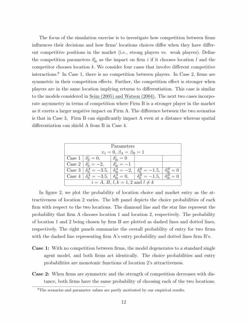
The focus of the simulation exercise is to investigate how competition between firms

influences their decisions and how firms’ locations choices differ when they have differ-

ent competitive positions in the market (i.e., strong players vs. weak players). Define

the competition parameters δilk as the impact on firm i if it chooses location l and the

competitor chooses location k. We consider four cases that involve different competitive

interactions.9 In Case 1, there is no competition between players. In Case 2, firms are

symmetric in their competition effects. Further, the competition effect is stronger when

players are in the same location implying returns to differentiation. This case is similar

to the models considered in Seim (2005) and Watson (2004). The next two cases incorpo-

rate asymmetry in terms of competition where Firm B is a stronger player in the market

as it exerts a larger negative impact on Firm A. The difference between the two scenarios

is that in Case 3, Firm B can significantly impact A even at a distance whereas spatial

differentiation can shield A from B in Case 4.

Parametersx1 = 0, βA = βB = 1

Case 1 δill = 0, δi

lk = 0Case 2 δi

ll = −2, δilk = −1

Case 3 δAll = −3.5, δA

lk = −2, δBll = −1.5, δB

lk = 0Case 4 δA

ll = −3.5, δAlk = 0, δB

ll = −1.5, δBlk = 0

i = A, B, l, k = 1, 2 and l 6= k

In figure 2, we plot the probability of location choice and market entry as the at-

tractiveness of location 2 varies. The left panel depicts the choice probabilities of each

firm with respect to the two locations. The diamond line and the star line represent the

probability that firm A chooses location 1 and location 2, respectively. The probability

of location 1 and 2 being chosen by firm B are plotted as dashed lines and dotted lines,

respectively. The right panels summarize the overall probability of entry for two firms

with the dashed line representing firm A’s entry probability and dotted lines firm B’s.

Case 1: With no competition between firms, the model degenerates to a standard single

agent model, and both firms act identically. The choice probabilities and entry

probabilities are monotonic functions of location 2’s attractiveness.

Case 2: When firms are symmetric and the strength of competition decreases with dis-

tance, both firms have the same probability of choosing each of the two locations.

9The scenarios and parameter values are partly motivated by our empirical results.

12

The choice probability of location 2 is again a monotonic function of its attrac-

tiveness as is the overall probability of entry. However, if we contrast this case to

Case 1, we observe that entry probabilities and the probability of choosing a more

attractive location are lower in this case where competitive effects exist. This ob-

servation indicates that each player makes a trade-off between the attractiveness of

location and the intensified competition. Competition makes the “good” locations

less attractive due to concerns about entry by rivals.

Case 3: When firm B is a stronger player and can impact firm A significantly at different

distances, firm A is much less likely to enter the market relative to firm B and

is correspondingly less likely to enter either of the two individual locations. In

this scenario, firm B deters firm A from entering at all unless location 2 becomes

sufficiently attractive at which point A’s desire to avail itself to the attractive

location overcomes its wariness about competing with B.

Case 4: When firm B is a stronger player, but competitive effects are local, the choice

patterns over the two locations differ dramatically across the two firms. The

stronger player (firm B) continues to be more inclined to choose location 2 as

location 2 becomes more attractive. The behavior of the weaker player (firm A)

is more interesting. Unlike in all other cases, its choice probability of location 1 is

not monotonically decreasing in the attractiveness of location 2. The bell-shaped

function reveals that the weak firm will sacrifice a good location in order to avoid

competition when location 2 is moderately attractive. In this situation, firm A

believes that firm B is sufficiently likely to enter the relatively attractive location 2

that A is willing to enter the less attractive location in order to insulate itself from

competition with B. However, as location 2 becomes more attractive, the attractive

market conditions eventually dominate the desire to differentiate implying that firm

A will also be more likely to choose the good location. Comparing cases 3 and 4, lo-

cation differentiation will be more attractive when the relative competitive position

changes with distance. In case 3, firm A cannot shield itself from competition by

differentiation and thus is unlikely to enter at all for moderately attractive markets.

This case would thus be associated with a dominant firm monopoly in moderately

attractive markets and agglomeration to good locations in very attractive markets.

Conversely, case 4 would be more likely to yield a spatially differentiated duopoly

in moderately attractive markets with agglomeration again occurring when one

location becomes sufficiently attractive.

13

These simulations indicate the potential impact of asymmetries in competitive effects

across locations as well as heterogeneity across firms. Most importantly, they indicate the

way in which the parameters of the payoff functions are empirically identified. As market

characteristics vary, different scenarios will yield different entry patterns. Intuitively,

the empirical analysis will then attempt to identify the relevant “case” and associated

parameter values that make observed entry patterns as close as possible to those predicted

by the model.

3 Data Description

We apply the model to the discount store industry. Discount stores originated in the late

1950s to offer general merchandise items at a substantial discount relative to conventional

department stores. For the most part, the industry is currently an oligopoly with three

dominant firms: Wal-Mart, Kmart, and Target. Interestingly, all three chains started in

1962 with Wal-Mart opening its first store in Rogers, Arkansas, Kmart in Garden City,

Michigan, and Target in Roseville, Minnesota. Over the past few decades, these firms

have obtained dominant positions in the retail world while expanding their operations

both domestically and internationally. They have also experimented with several other

retail formats, most prominently the supercenter which combines a full-service grocery

store and a general merchandise outlet. In addition, these stores include several ancillary

services such as pharmacies, dry cleaning, vision centers, automotive care centers, hair

salons, and income tax preparation resources (in season) to provide consumers with a

true “one-stop” shopping environment.

Besides physical store locations considered in this study, the firms have also looked

to differentiate themselves in other dimensions. For instance, with its EDLP strategy

and the “Always Low Prices, Always” slogan, Wal-Mart has tried to establish itself as

the low price leader in the industry. It has also emphasized the supercenter format

more than Target and Kmart with approximately half of its 3,000 stores selling grocery

products. Similarly, Target has looked to place itself in a niche as an “upscale” discounter

with higher-end products. It has partnered with several designers to offer contemporary

merchandise, runs its own Target Guest credit card, and heavily promotes its nationwide

bridal and baby shower gift registries. Target’s panache is reflected in the pop-culture

use of a French-influenced pronunciation for its name (Tar-jay).10

10For a detailed background on these firms, interested readers are referred to Zhu, Singh, and Manuszak(2005) and three recent books on each firm: The Wal-Mart Decade: How a New Generation of LeadersTurned Sam Walton’s Legacy into the World’s #1 Company (Robert Slater) Portfolio Hardcover (2003);

14

In this study, we use a novel dataset that includes locations (street addresses and

zip codes) of all stores in operation as of 2003 for Wal-Mart, Kmart, and Target. In

addition, we observe store format information, discount store versus supercenter. The

total number of stores belonging to each chain is presented in Table 1. We do not consider

Sam’s Club as its main competitors are other membership clubs such as Costco and BJ’s.

Wal-Mart is the largest player with almost 3000 total stores and, as mentioned above, has

stores equally split between the two store formats. By contrast, Kmart and Target are

relatively minor players in the supercenter format. In Table 2, we show the distribution

of stores for these three chains across the country. Not surprisingly, the highest number

of stores are found in the two largest states, California and Texas. The three chains

have the highest share (in terms of number of stores) in their states of origin: Kmart in

Michigan, Wal-Mart in Arkansas, and Target in Minnesota. The chains also tend to have

a disproportionate share of stores in the states neighboring their headquarters.

Our main objective in this paper is to analyze the factors underlying the entry and

location choices of these firms and to infer competitive interaction parameters based on

their revealed preferences. For the purpose, we need to partition the United States into

small markets and each market into smaller neighborhoods. While various market def-

initions are possible, a practical consideration is the availability of data that capture

demand and cost conditions at each location. Our approach relies on census-delineated

lines to define the individual markets as well as the locations within markets. In par-

ticular, we use counties as our definition of markets and census tracts within counties

as locations.11 Census tracts are small, relatively permanent geographic entities within

counties (or the statistical equivalents of counties) delineated by a committee of local

data users and tend to be fairly homogeneous with respect to population characteristics,

economic status, and living conditions. In the empirical estimation, neighboring loca-

tions will be defined to be all locations within a given distance range which we specify

below.12

On Target: How the World’s Hottest Retailer Hit a Bullseye ( Laura Rowley) Wiley (2003); Kmart’sTen Deadly Sins: How Incompetence Tainted an American Icon, (Marcia Layton Turner) John Wiley &Sons (July 18, 2003)

11For very large urban counties (for example LA county), we use the first three digits of the tractnumber to create sub-markets. The complete census tract ID is defined as follows: SS-CCC-TTTTTT,where the first two digits “SS” represents State FIPS code, the next three digits “CCC” representsCounty FIPS Code, and the last six digits “TTTTTT” is the census tract number. This definitiondefines a market as the tracts within a county with the same first three digits in their tract numbersand all six digit codes as locations.

12Two recent applications (Seim 2005, Watson 2004) also use census tract as locations although theirdefinition of market is mid-size cities. We could alternatively define markets based on 4-digit zip codesand locations based on 5-digit zip codes. However, this approach would be problematic since zip code

15

In Table 3, we present the competitive configurations across US counties along with

some characteristics of those markets. The letters W, K, and T represent the presence

of Wal-Mart, Kmart, and Target firms in the market where, for the sake of brevity, we

have omitted information associated with store format. For instance, (0,0,0) represents

markets with no firms; (W,0,0) are Wal-Mart monopoly counties; (W,K,0) are duopoly

counties of Wal-Mart and Kmart, and so on. A few patterns are apparent from the

numbers presented in Table 3. First, markets with no firms have significantly smaller

populations compared to markets with at least one firm. Second, Wal-Mart operates as

a monopolist in a larger number of counties than its rivals. As the associated market

populations suggest, this reflects its ability to operate in smaller markets. Third, Tar-

get stores generally operate in markets with larger population and significantly higher

incomes compared to Wal-Mart and Kmart which is consistent with the anecdotal ev-

idence discussed above. Finally, the population numbers generally indicate that larger

markets are required for additional entry.

Table 4 lists the full set of variables used in the estimation where we separate the

variables that are observed at the market, location, and firm level. We also present the

overall averages and means by MSA and rural Non-MSA markets. The average market

size in our data is approximately 700 square miles although the rural markets tend to

be larger in size than MSA markets. In terms of population we find the opposite as

MSA markets have double the number of people reflecting that the urban areas are quite

densely populated compared to rural markets. We can also see that MSA markets tend

to have higher retail wages and more retail establishments. The next row shows the

number of census tracts within a market. The average number of locations in a market

ranges from approximately six in the rural markets to over nine in MSA markets.

The next panel of the table describes the location-specific variables. The first two

rows are the populations within a two and a two-to-ten mile radius of the location. We

find a similar pattern to the market-level characteristics as MSA markets have signifi-

cantly larger population numbers than the non-MSA markets. The next three variables

%Novehicle, %Child, and HHsize are the percent of population with no vehicles, per-

cent of population with children in the family, and household size respectively. These

three variables do not differ substantially across MSA and rural markets. However, MSA

locations do tend to have higher levels of income and house values as well as a higher

proportion of younger and educated population.

The last set of variables are firm-level variables that are specific to each location. In

classification yields markets that are not contiguous.

16

particular, the data include distances from locations to the headquarters and distribution

centers of firms. These variables were created to proxy for logistical issues in a firm’s

location decisions and, as we shall see below, tend to be quite important.

4 Empirical Application

4.1 Estimation Issues

The model described in (4) is very flexible as it allows for competition effects to be

asymmetric across firms and for the intensity of competition to depend on proximity.

However, the general model has a large number of competitive parameters (the δ’s) to be

estimated. Without any constraints the number of competitive interaction parameters is

Lm × Lm × N × (N − 1) which grows quickly even with a small number of players and

locations. For instance, with three players and ten locations, the number of competition

parameters is 600. Clearly, some restrictions on the number of parameters are required.

To deal with this difficulty, we create discrete distance bands and assume that the com-

petitive intensity between players is the same as long as they are within the same band.13

In the estimation, we categorize the distance between locations into three bands: less

than 2 miles, 2 to 10 miles, and more than 10 miles. Note that this approach implies

that if δii′0 is the competitive impact of firm i at location k1 that is within 2 miles from

location l chosen by player i′, then the competitive effect is still δii′0 were firm i to choose

another location k2 that is also within 2 miles of l. In other words, in this framework

the intensity of competition is determined by the distance between locations and not

the identities of those locations. The advantage of the approach is that the number of

parameters reduces significantly. For instance, using the three distance bands described

above, the total number of parameters is reduced to 3× 3× 2 = 18.

The model can be summarized as follows:

πiml = ximlβi −∑i′ 6=i

B−1∑b=0

Lm∑k=1

δii′bai′mk1 (k ∈ bl) + ξm + εiml (8)

13We assume that firms are located at the centroid of the location, i.e., census tract. We calculate thedistance between locations using the Haversine Formula. Based on latitude-longitude coordinate data,the distance between two points, a and b, is given by

da,b = 2R arcsin[min

((sin (0.5 (latb − lata)))2 + cos (lata) cos (latb) (sin (0.5 (lonb − lona)))2

)0.5

, 1]

where R = 3961 miles denotes the radius of the earth. A similar approach of creating competitive effectsusing distance bands is used by Seim (2005) and Watson (2004).

17

where B is the total number of bands and 1 (k ∈ bl) is an indicator function with

1 (k ∈ bl) =

1 if db ≤ dlk < db+1

0 otherwise, (9)

where db and db+1 denote cut-offs that define a distance band. In other words, 1 (k ∈ bl) =

1 whenever location k is in distance band b relative to location l.

The parameters to be estimated are θ = β, δ, σ where β captures firms’ preferences

over the exogenous market conditions, δ reflects competitive effects across firms and

locations, and σ measures the importance of the market level random component. To

estimate the model, we nest the fixed point algorithm in (5) into a maximum likelihood

routine. For a given set of values of the parameters and the market, location, and

firm specific exogenous variables, the system of equations in (5) is solved numerically

for its fixed point for each market. The fixed point is a vector with∑

i Lim elements

which represent the probability of each location being chosen by each firm. Given those

probabilities, P (ym) =∏

i P (yim) is the probability of the equilibrium realization that

is consistent with the observed market outcome.The likelihood function is given by

L (y, X, ξ; θ) =M∏

m=1

P (ym|Xm, ξm; β, δ) . (10)

The unconditional likelihood then involves integrating over the distribution G (.) of the

unobserved market component ξm, where ξm is assumed normally distributed with vari-

ance σ in our application.

L (y, X; θ) =M∏

m=1

∫P (ym|Xm, ξm; β, δ) dG (ξm|σ) , (11)

where ym = (yWm, yKm, yTm) are observed actions taken by Wal-Mart, Kmart and Target.

Computationally, the model is quite complicated. To simplify the estimation, we em-

ploy a simulated maximum likelihood routine as follows.14 Given a set of parameter val-

ues and a vector of simulated draws with standard normal distribution ς =(ς1, ς2, ..., ςR

)14One problem of the likelihood approach is that there might be multiple equilibria in the incomplete

information game. However, as long as the strength of competition effect is moderate, the equilibriumcan be solved uniquely. We show analytical and simulation results in the appendix. An alternativeestimation strategy is to use a two-stage pseudo MLE procedure described in Bajari, Benkard and Levin(2005), which does not require computation of equilibrium outcomes. The approach involves two stepswhere the first step is to recover the agents’ belief on their competitors behavior, which in practice,involves regression of observed actions on state variables, such as demand and cost shifters.Suppose θ1

are the parameters we obtained from the first stage regression and θ2 are the primitive parameters infirms’ payoff functions. The first-stage parameters can be estimated either nonparametrically or someparametric model (for example multinomial logit) when the dimension of the problem is large. Given the

18

for the unobserved market characteristic, we begin with an initial guess of the choice

probability for each firm P 0m ∈ [0, 1]

∑i Lim in each market. We then calculate each firm’s

expected payoff for each location conditional on its beliefs about its competitors’ location

choice probability P 0−im. For each random draw ςr, we solve the fixed point problem (5)

by successive approximation to obtain the Bayesian Nash equilibrium probabilities P rm.

We then repeat the procedure R times to find the Bayesian Nash equilibrium for each

random draw. The predicted probability of the observed outcome is approximated by∫P (ym|Xm, ξm; β, δ) dG (ξm|σ) =

1

R

R∑r=1

P rm (ym) . (12)

We then use the simulated probabilities in a log-likelihood function:

θ = arg maxθ

LL (y, X; θ) =M∑

m=1

ln

[1

R

R∑r=1

P rm (ym)

]. (13)

4.2 Results

We include a variety of variables that capture demand, cost, and logistical factors that

could be important in a firm’s location decision. Since these factors might operate dif-

ferently in large MSA markets compared to rural areas, we divide the sample into MSA

and non-MSA markets and estimate separate models for each. We also allow Wal-Mart

to choose between its discount store and supercenter formats. As noted in the data sec-

tion above, the other two players mainly operate discount stores so we ignore the format

choice decisions for these players.

In Table 5, we report the parameter estimates for MSA markets.15 We will focus on

those estimates since similar results obtain for non-MSA markets as displayed in Table

predicted probabilities from the first stage, Pi

(ai|x, θ1

), the structural parameters θ2 can be recovered

by maximizing the following likelihood.

L(θ1, θ2

)=

N∑m=1

I∑i=1

log

exp(∑

a−imfim (aim, a−im, xm; θ2) P−im

(a−im|xm, θ1

))1 +

∑a′im

exp(∑

a−imfim (a′im, a−im, xm; θ2) P−im

(a−im|xm, θ1

))

The estimation procedure has computational advantage over the full MLE in that it does not requireto solve for fixed point problem to get the equilibrium outcomes. The first stage estimation recoversequilibrium beliefs from the data directly. However, the cost of the two-stage approach is that it does notuse all the information available from the model, especially in the first stage estimation. In addition itassumes that all the relevant state variables are observed during the first stage estimation. In practice,there are a number of factors that are observed by firms, but not by analysts. As noted below, theunobserved market characteristics, ξm are found to be quite significant in the empirical application.

15As a caveat, it should be noted that the parameters should be interpreted with care due to both

19

6. Not surprisingly, we find that closer population contributes more to profitability that

more distant population as reflected in the lower value of the coefficients for population

in more distant bands. However, the parameters for distant population are significantly

larger for Wal-Mart, particularly for its supercenter format. This finding suggests that

the trading area for Wal-Mart is larger than that of its rivals. The estimated effect

of population density is negative for all players except Kmart. While this may seem

counterintuitive, note that population density is measured at the specific location cell

level, while the population measures include populations from the immediate as well as

neighboring locations that fall within the respective distance band. Since the discount

stores tend be large in size, it is not necessarily surprising that population density in

the immediate location is low. In addition, a location with high population density may

have high real estate costs implying that the chains would prefer locations with lower

immediate population density, but higher overall surrounding population.

The next two variables, %Child and %Novehicle, represent the percent of population

with children under the age of 18 and percent of population with no vehicles. The

parameters for %Child are positive for Wal-Mart and Target, but are insignificant for

Kmart. Thus, both Wal-Mart and Target stores prefer markets where a larger proportion

of families have kids. In relative terms, the impact is larger for Wal-Mart, particularly

for its supercenter format. The parameter for %Novehicle is significantly negative for all

stores which is intuitive as these stores are built with large parking lots that are generally

inaccessible without vehicles. The next two demographic variables are median income

and education measured as the percentage of population with a college degree. These

two variables reveal some interesting differences across firms. The income parameter is

negative for both Wal-Mart formats, insignificant for Kmart, and positive for Target.

These results suggest that, all else equal, Wal-Mart enters markets with lower incomes

while Target stores prefer high income areas. In addition, Target stores tend to have a

more educated population base. These results are consistent with common perceptions

of the positioning and target audiences of these stores. For example, as discussed above,

Target has historically attempted to position itself as an upscale discounter that caters

to a higher income and more educated clientele than its competitors. Similarly, lower

income levels in Wal-Mart locations are consistent with Wal-Mart’s every day low pricing

and value positioning.

the reduced form nature of the payoff function and the fact that, as with any discrete choice model, theparameters are only estimated up to an unknown positive scale factor. While the latter point implies thatthe absolute magnitudes of the estimates are difficult to interpret, their signs and relative magnitudesare directly interpretable.

20

The next variable HouseValue is the median house value which ideally will capture

the impact of real estate prices. The coefficient is negative for Wal-Mart discount store,

positive for its supercenter format, and insignificant for Kmart and Target. However, the

instability of these results appear to indicate that residential house value is in fact an

inaccurate proxy for commercial land value. The coefficients for retail wages are negative

and significant indicating that all firms strongly prefer markets with lower wages. This

is not surprising since labor tends to account for a significant proportion of operational

costs in retailing. The variable “num of retailers” is the total number of other retailers

and captures the general business density at a location. Note that these retail stores

are considered to be non-strategic players in our model even though some of them may

actually compete with the three discount stores. The coefficient is negative for the two

Wal-Mart stores and positive for Kmart and Target. This suggests that Wal-Mart tends

to prefer stand alone locations while its competitors are more likely to be surrounded by

other businesses.

The last two variables Dist HQ and Dist DC are the distance of different market

locations from the headquarters and nearest distribution center of a firm. Unlike all

the variables discussed above, these distance measures are firm-specific. The negative

coefficients for distance to headquarters suggests that, all else equal, firms prefer markets

that are closer to their respective headquarters. This is consistent with the distribution

of stores across states reported in Table 2. Looking at the distance to distribution center,

we find that Wal-Mart, particularly for its supercenter format, prefers locations that are

closer to its distribution center. This is not surprising as Wal-Mart is well known for its

efficiency in distribution, and a large part of its success as a retailer has been attributed

to these logistical efficiencies.16

Looking at the competitive interaction parameters, some interesting patterns emerge.

As expected, all parameters are negative indicating that presence of rivals reduce a firm’s

profits. However, proximity to competitors is an important determinant of profitability

as the competition effect diminishes with distance. For instance, the point estimates

suggest that the impact of Kmart on a Wal-Mart’s discount store is approximately 45%

lower when it is located more than ten miles away instead of being located in the imme-

diate neighborhood. This decreasing relationship between distance and competition is

consistent across all firms and formats which suggests strong returns to spatial differen-

16According to an independent study by McKinsey &Co., Wal-Mart’s efficiency gains were the sourceof 25% of the entire U.S. economy’s productivity improvement from 1995 to 1999. “Can Wal-Mart getany bigger” Time Magazine (Vol. 161, issue 2, 2003)

21

tiation in this industry as firms can shield their profits by choosing sufficiently different

locations. Looking at the competitive effects across firms, we find strong asymmetries

in the competitive interaction parameters. For example, looking at Kmart and the two

Wal-Mart formats, we find that while Kmart substantially impacts Wal-Mart when it is

in close proximity, the effect is significantly lower than the effect of Wal-Mart on Kmart.

Similarly, when Kmart is located beyond ten miles, its effect on Wal-Mart’s discount

store and supercenter are approximately one-fourth of the impact that the Wal-Mart

stores have on Kmart at a similar distance. Target stores fare well in the face of com-

petition from other discount stores except when the competitors are in close proximity.

However, the chain appears vulnerable to Wal-Mart’s supercenter format. Perhaps most

interesting, the impact of Wal-Mart supercenter appears to decline less rapidly with dis-

tance when compared to the effect of any of the other firms. This finding suggests that

Wal-Mart’s supercenter format yields a substantially larger market area relative to other

formats as even competitors which are relatively far from a supercenter are not insulated

from competition with it.

To better interpret the competition effects, one can calculate measures on the demand

reduction in terms of population when a competitor moves into a location, holding all

else constant. For example, moving a new Wal-Mart discount store within 2 miles of

Kmart is equivalent to reduction of 33,600 in population for Kmart in the immediate

neighborhood. The effect of a new Kmart on a Wal-Mart discount store is only 15,800

which is less than half the impact that Wal-Mart has on Kmart. If a new Wal-Mart

supercenter moves in, even in a far away location (beyond 10 miles), it is equivalent to a

reduction in population of 24,000 for Kmart and 18,900 for Target. The corresponding

numbers for a Wal-Mart discount store are 20,900 for Kmart and 2,000 for Target. Thus,

Kmart seems vulnerable to both formats of Wal-Mart even in far away locations, while

Target fares well when faced with a distant Wal-Mart discount store, but is still affected

strongly by a Wal-Mart supercenter. In fact, the impact of Target is stronger on Kmart

and Wal-Mart’s discount store when located more than 10 miles away rather than the

other way around.

4.3 Varying Market Conditions and Equilibrium Outcomes

The model parameters can be used to predict the equilibrium market structures for differ-

ent sets of market conditions and provide insights on how these firms shield themselves

from competition by spatial differentiation. For instance, consider a market with two

possible locations that are 10 miles apart, and three potential competitors: Wal-Mart

22

supercenter, Kmart, and Target. Further, suppose the population in location 1 is 30,000

and income is at the mean level in the population which is normalized to zero. In ad-

dition, all other variables are set at their population mean levels. Figure 3 displays the

predicted market structures as population and income change in location 2. Note that

the parameter estimates of the latent payoff functions suggest that the impact of the two

variables may work differently for different firms. In particular, while all firms prefer

increase in population especially in the immediate location, Target is the only firm that

prefers higher income levels. The darker shade represents choice of location 1, lighter

shade the choice of location 2 (Red and Blue if viewed in color), and non-shaded ar-

eas represent situations where firms stay out of the market. The left panel shows the

predicted outcomes without considering competition, while the right panel shows the

equilibrium structures after taking competition into account. Figure 3-1a shows that

when firms do not compete, no entry and monopoly outcomes are rare as all three firms

are willing to enter the market with moderate increases in population and income levels.

Figure 3-1b shows that the region of no-entry and monopoly increase dramatically once

we account for competition. Moreover, the occurrence of oligopoly is much less prevalent

and only arises at significantly high population and income levels.

In Figures 3-2a to 3-4b, we show how the predicted entry and location choices vary

by individual firms. Comparing individual firms under competition and no-competition,

some interesting patterns emerge. Wal-Mart’s no-entry region, while larger under compe-

tition compared to the no-competition case, is relatively small compared to its rivals. The

impact of competition is highest on Kmart as it gives up the majority of the space that it

would have occupied if competitive concerns were irrelevant. Looking at Wal-Mart’s lo-

cation choices, we observe that as the income in location 2 increase above a certain point,

Wal-Mart is willing to enter the market by switching to location 1. On the other hand,

both Target and Kmart prefer not to enter the market altogether with moderate market

conditions and choose location 2 as it becomes sufficiently attractive. These results are

primarily driven by Wal-Mart supercenter’s ability to enter markets with lower popu-

lation levels, attract population from further away locations, and its ability to impact

competitors even when it is located far away. Comparing the monopoly region in Figure

3-1b with those of three firms under competition (Figures 3-2b, 3-3b, 3-4b), we can see

that majority of the monopoly region is occupied by Wal-Mart with a small region (those

with moderate population and very high income) being Target’s monopoly. Kmart on

the other hand is rarely able to operate as a monopolist. Of course these predictions

would change at different values of the other market variables. For example, Kmart may

23

have monopoly markets in regions close enough to its headquarters.

Overall, the results show that all firms exert a strong negative impact on its competi-

tors when they are in close proximity and that this effect decreases with distance to rivals.

Wal-Mart’s supercenter format is found to be the most formidable player as it strongly

impacts competitors even from a distant location. Not surprisingly, in our empirical data

we observe a large number of monopoly markets for Wal-Mart supercenter. We also find

asymmetries across players in terms of exogenous market characteristics. In Table 7, we

show the parameter estimates from a model that ignores player identities. With minor

differences, this is the model used by Seim (2005) and Watson (2004) in their applica-

tions to video rental stores and eyewear retailers respectively. Several similarities exist

in the parameter estimates with the full model presented above. For instance, payoffs

are higher with population closer the firm’s location. Similarly, the competitive effect

decreases with distance to rivals suggesting returns to geographical differentiation. How-

ever, this model can not discern the differences across firms with regards to preference for

exogenous variables as well as competition effects. While this model may be reasonable

in industries with small local players who are reasonably homogeneous in many respects,

in our application the impact of income, education, business density, distance to distri-

bution center, and competition is found to be quite different based on the identities of

individual players.

5 Conclusion

In this paper we study the strategic entry and location choice decisions in the retail

discount industry. Using a novel data set that includes the store locations and the ac-

companying market conditions for all stores belonging to Wal-Mart, Kmart, and Target

chains, we study the factors determining firm’s entry and location choices. The model

is set up as an incomplete information game between the three players where firms are

assumed to have private information on their own profitability but observe only the dis-

tribution of their rivals’ profitability. The model incorporates asymmetries related to

the identity of the firms by allowing the competitive effects and preference for exoge-

nous market conditions to be firm-specific. The incomplete information setup provides

a tractable model for studying the complex interactions of optimal site selection as a

trade-off between proximity to good markets and increased competition with rivals in

these prime locations.

Results show that population in closer distance bands to firm’s location contribute

24

more to profitability than population in distant locations. All firms are found to prefer

markets with lower retail wages, markets where larger proportion of families have kids

and vehicles, and markets that are closer to their respective headquarters. We also find

significant differences across firms in certain demand characteristics. For instance, Wal-

Mart and Kmart stores are found to prefer markets with lower income levels, while Target

prefers markets with higher income and education levels. These results seem consistent

with common perceptions of these stores. We also find that Wal-Mart, particularly for

its supercenter format, gives strong weight to locations that are closer to its distribution

center, reflecting its logistical efficiencies. In terms of the competitive interaction param-

eters, we find that proximity to competitors an important determinant of profitability.

All firms are found to exert a strong negative impact on their competitors when they

are in close proximity, but the effect goes down with distance to rivals suggesting strong

returns to spatial differentiation in this industry. However, looking at the competitive

effects across firms, we find strong asymmetries in the competitive interaction parame-

ters. For example, while Kmart is able to impact Wal-Mart strongly when it is in close

proximity, its effect is significantly lower than what Wal-Mart exerts on Kmart’s payoffs.

Target stores are found to fare well under competition from other discount stores except

when these competitors are in close proximity. Wal-Mart’s supercenter format is found

to be the most formidable player as it is able to impact the competitors strongly even

when it is located far away.

There are of course several caveats to this study and directions for future research.

First, the incomplete information assumption in a static game implies that players are

allowed to have ex post regret about their decisions, which naturally leads to dynamic

considerations (Aguirregabiria and Mira 2004, Pakes et al. 2004). While applications

of multi-agent dynamic games pose significant computational challenges, they may pro-

vide insights into the rich dynamics inherent in strategic decisions like market entry and

exit that are lost in a static setting. Second, to reduce the number of parameters we

resorted to three distance bands that could have been made finer at the cost of addi-

tional parameters. Finally, in our application the only unobservables that are correlated

across players are market specific that do not differentiate between locations within a

market. Location specific unobservables can obviously be incorporated in the model

at the expense of additional computational burden. Although addressing many of these

shortcomings pose significant challenges in terms of data requirements and computations,

with advancements in computing power these hurdles can be overcome in the future.

25

Appendix: Equilibrium Properties of Incomplete In-

formation Games

A well-known problem with multi-agent discrete games is that they have non-existence ofpure strategy equilibria and multiple equilibria in which certain values of the underlyinglatent payoffs could simultaneously be consistent with more than one equilibrium out-come. For existance, researchers generally assume that the data is generated by a purestrategy equilibrium and that the model satisfies restrictions sufficient to guarantee theexistence of at least one such equilibrium. In the current application, since equation(6) isa continuous mapping from a probability space to itself, the existence of a solution of (6)can be proved from Brouwer’s Fixed Point Theorem. However, the uniqueness of such asolution is not guaranteed. The game will have multiple equilibria if, for given parameterθ, more than one value of P satisfies (6) in which case the likelihood function is not welldefined. Aradillas-Lopez (2005) discusses the sufficient conditions for the uniqueness ofequilibrium of incomplete information game and points out that the conditions for exis-tence of a well-defined likelihood function are generally weaker in incomplete informationgame than in the complete information version of the game.

Heckman (1978) studies the general class of simultaneous equation qualitative re-sponse models and shows that if the distribution of the unobservables is continuous withunbounded support, a necessary and sufficient condition for the model to have a uniqueequilibrium for any values of exogenous variables is that the model is recursive. Thoughuseful in some applications, this condition implies setting some strategic interactionsparameters (which are of main interest) to zero. Instead, researchers have generallyadopted one of the two approaches to deal with multiple equilibria problem. First, mod-els sometimes yield a prediction for some outcome that is unique across all equilibria. Forinstance, BR (1990, 1991) and Berry (1992) ignore the identities of the players that entera market and only consider the total number of entrants, an outcome for which theirmodels yield a unique prediction. Alternatively, some papers impose additional struc-ture on the model that guarantees equilibrium uniqueness. For example, Zhu, Singh, andManuszak (2005) consider sequential move games that yields additional conditions for anoutcome to be a subgame perfect Nash equilibrium.

In this appendix, we study the equilibrium properties for the model proposed inSection 2. We begin with a proof on the sufficient conditions of uniqueness for the twoplayer - two action game and then rely on simulation techniques for a more complexgame, i.e., when the action space or the number of players becomes larger.

Consider a simple 2 × 2 game with two players and two possible actions: in or out.Firm i’s payoff of entry is

πi = xiβi − δip−i + εi, i = 1, 2, (A1)

where p−i is the entry probability of i’s competitor, and εi is the private information heldby firm i and is type 1 extreme value distributed. Similar to the discussion on equation(7), the BNE is obtained by solving the following two simultaneous equations:

p1 =exp (x′1β1 − δ1p2)

1 + exp (x′1β1 − δ1p2),

and

p2 =exp (x′2β2 − δ2p1)

1 + exp (x′2β2 − δ2p1).

26

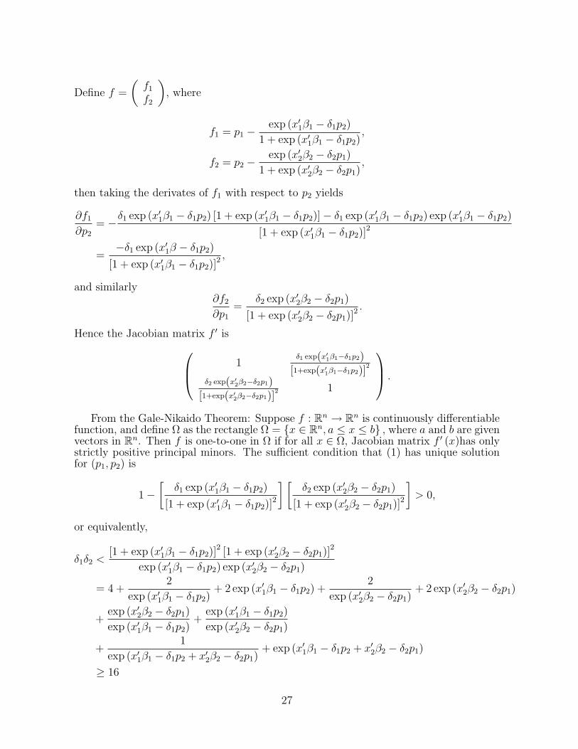
Define f =

(f1

f2

), where

f1 = p1 −exp (x′1β1 − δ1p2)

1 + exp (x′1β1 − δ1p2),

f2 = p2 −exp (x′2β2 − δ2p1)

1 + exp (x′2β2 − δ2p1),

then taking the derivates of f1 with respect to p2 yields

∂f1

∂p2

= −δ1 exp (x′1β1 − δ1p2) [1 + exp (x′1β1 − δ1p2)]− δ1 exp (x′1β1 − δ1p2) exp (x′1β1 − δ1p2)

[1 + exp (x′1β1 − δ1p2)]2

=−δ1 exp (x′1β − δ1p2)

[1 + exp (x′1β1 − δ1p2)]2 ,

and similarly∂f2

∂p1

=δ2 exp (x′2β2 − δ2p1)

[1 + exp (x′2β2 − δ2p1)]2 .

Hence the Jacobian matrix f ′ is 1δ1 exp(x′

1β1−δ1p2)[1+exp(x′

1β1−δ1p2)]2

δ2 exp(x′2β2−δ2p1)

[1+exp(x′2β2−δ2p1)]

2 1

.

From the Gale-Nikaido Theorem: Suppose f : Rn → Rn is continuously differentiablefunction, and define Ω as the rectangle Ω = x ∈ Rn, a ≤ x ≤ b , where a and b are givenvectors in Rn. Then f is one-to-one in Ω if for all x ∈ Ω, Jacobian matrix f ′ (x)has onlystrictly positive principal minors. The sufficient condition that (1) has unique solutionfor (p1, p2) is

1−[

δ1 exp (x′1β1 − δ1p2)

[1 + exp (x′1β1 − δ1p2)]2

] [δ2 exp (x′2β2 − δ2p1)

[1 + exp (x′2β2 − δ2p1)]2

]> 0,

or equivalently,

δ1δ2 <[1 + exp (x′1β1 − δ1p2)]

2 [1 + exp (x′2β2 − δ2p1)]2

exp (x′1β1 − δ1p2) exp (x′2β2 − δ2p1)

= 4 +2

exp (x′1β1 − δ1p2)+ 2 exp (x′1β1 − δ1p2) +

2

exp (x′2β2 − δ2p1)+ 2 exp (x′2β2 − δ2p1)

+exp (x′2β2 − δ2p1)

exp (x′1β1 − δ1p2)+

exp (x′1β1 − δ1p2)

exp (x′2β2 − δ2p1)

+1

exp (x′1β1 − δ1p2 + x′2β2 − δ2p1)+ exp (x′1β1 − δ1p2 + x′2β2 − δ2p1)

≥ 16

27

Hence as long as the interaction term of the competition intensity δ1δ2 is below 16, theuniqueness of the Bayesian Nash equilibrium is ensured in this 2× 2 game.

The message from the simple example above is that as long as the strength of strategicinteraction is within a certain range, equilibrium is unique. As the game becomes morecomplex, i.e., the action space or the number of players gets larger, the matrix algebrabecomes cumbersome. We rely on simulation technique to investigate the uniquenessproperty of incomplete information games. In the simulation, We are interested in howthe equilibrium uniqueness property is related to (1) the variation of market character-istics across locations (choice alternatives), (2) the heterogeneity across players, and (3)the magnitude of competition effect. This simulation exercise is motivated by Bayer andTimmins (2004). We assume

• There are two locations in the market, location 1 and location 2.

• There are two players A and B who decide whether to enter the market or not andwhich location to choose.

• The competition between players at the same location is stronger than the compe-tition between players from different locations.

Players’ payoff functions are assumed to be:

πil = xlβi −2∑

k=1

δilkPi′l + εil, i, i

′ ∈ A, B and i 6= i′, l, k = 1, 2

where δilk denotes the how firm i’s payoff at location l is affected by its competitor’s entry

of location k and δill ≥ δi

ll′ , where l′ 6= l. εil are iid type one extreme value distributed.We normalize x1 = 1, βA = 1, and change x2 from 1 to 10 and βB from 1 to 2. The

ratio x2/x1 captures the variation of market conditions across locations. The larger theratio, the more different the two locations are. Similarly, the ratio βB/βA representsthe level of firm heterogeneity. Given the same market conditions, firms’ profitabilitywill be different due to their preferences of those market factors. Given x1, x2, β1, β2

and δilk, the fixed points of the probability vector (P1A, P2A,P1B,P2B) are solved from

different starting values: (0 0 0 0)′, (0 0 1 0)′, (0 0 0 1)′, (1 0 0 0)′, (1 0 1 0)′, (1 0 0 1)′,(0 1 0 0)′, (0 1 1 0)′, (0 1 0 1)′. The discussion on why one should choose those points asstarting points to test equilibrium multiplicity can be found in Bayer and Timmins(2004).As we change δA

11 from 0 to 100, and find δill, such that as δi

ll > δill, we start to observe

multiple fixed points for a particular combination of x1, x2, β1, β2. In figure 4 and figure5 we plot how δi

ll changes as x2/x1 and β2/β1 changes under two scenarios:Case 1: Symmetric competition , δA

lk = δBlk, δi

ll′ = 12δill

Case 2: Asymmetric competition: δAlk = 2δB

ik, δill′ = 1

2δill

In the first case, firms are symmetric in terms of competition, while in the secondscenario Player B is stronger than player A in the sense that it exerts stronger negativeimpact on its competitor. The competition intensity is weaker if two players choosedifferent locations. Comparing the plot for case 2 and that for case 1, we can findthat the threshold for case 2 is larger. The reason is that the uniqueness conditions aredetermined by the interaction terms of the competition intensity. Hence the range forthe competition intensity of δ1

11 is larger if δAlk > δB

lk.The results from simulation can be summarized as follows. First, as long as the

strength of competition effect is moderate, there is a unique equilibrium in the incom-plete information game. Second, there exists a thereshold δA

lk such that when δAlk > δA

lk,

28

one starts to observe multiple equilibrium given the location characteristics and firms’preference of those market characteristics. We find that as the variation of market char-acteristics increases, the threshold δA

lk increases. Put another way, the multiple equilibriais less likely to be observed when there is larger variation across locations. This find-ing is consistent with Seim(2001). Finally, as the asymmetry between players increasesboth in terms of their preference to market conditions (βB/βA) and the asymmetric ofcompetition effect, the threshold δA

lk becomes higher.

29

Reference

1. Aguirregabiria, V. and P. Mira (2004), “Sequential Estimation of Dynamic DiscreteGames,” Working Paper, Boston University.

2. Aradillas-Lopez, A. (2005), “Semiparametric Estimation of a Simultaneous Gamewith Incomplete Information.” Working Paper, Berkeley.

3. Arnold, S. J., T. H. Oum and D. J. Tigert (1983), “Determinant Attributes inRetail Patronage: Seasonal, Temporal, Regional and International Comparisons,”Journal of Marketing Research, 20 (May) 149-57.

4. Bajari P., L. Benkard, and J. Levin (2005), “Estimating Dynamic Models of Im-perfect Competition,” Working paper, Duke.

5. Bajari, P., H. Hong, J. Krainer, and D. Nekipelov (2005), ‘Estimating StaticModels of Strategic Interactions’, Working Paper, University of Michigan.

6. Bayer P. and C. Timmins (2004), “ On the Equilibrium Properties of LocationalSorting Models,” Working Paper, Yale University.

7. Berry, S. T. (1992), “Estimation of a Model of Entry in the Airline Industry,”Econometrica, 60 (4), 889-917.

8. Besanko, D., J. P. Dube, and S. Gupta (2003), “Competitive Price Discrimina-tion Strategies in a Vertical Channel Using Aggregate Retail Data,” ManagementScience, 49 (9), 1121-38.

9. Besanko, D., S. Gupta, and D. Jain (1998), “Logit Demand Estimation underCompetitive Pricing Behavior: An Equilibrium Framework,” Management Science,44 (11), 1533-47.

10. Bresnahan, T. F. and P. C. Reiss (1987), “Do Entry Conditions Vary across Mar-kets,” Brookings Papers on Economic Activity (3), 833-81.

11. — (1990), “Entry in Monopoly Markets,” Review of Economic Studies, 57 (4),531-53.

12. — (1991), “Entry and Competition in Concentrated Markets,” Journal of PoliticalEconomy, 99 (5), 977-1009.

13. — (1991), “Empirical-Models of Discrete Games,” Journal of Econometrics, 48(1-2), 57-81.

14. Brown, S. (1989), “Retail Location Theory: The Legacy of Herald Hotelling,”Journal of Retailing, 65, 450-70.

15. Chan, T., V. Padmanabhan, and P.B. Seetharaman (2005) “Modeling Locationsand Pricing Decisions in the Gasoline Market: A Structural Approach” WorkingPaper, Olin School of Management

16. Chintagunta, P. K. (2002), “Investigating Category Pricing Behavior at A RetailChain,” Journal of Marketing Research, 39 (2), 141-54.

30

17. Chintagunta, P., J. P. Dube, and V. Singh (2003), “Balancing Profitability andCustomer Welfare in a Supermarket Chain, Quantitative Marketing & Economics,1(1), 111-47.

18. Chintagunta P., T.Erdem, P. Rossi and M. Wedel “Structural Modeling in Market-ing: Review and Assessment,” Marketing Science, forthcoming.

19. Ciliberto, F. and E. Tamer (2004), “Market Structure and Multiple Equilibria inAirline Markets,” Working Paper, Princeton University.

20. Craig, S. C., A. Ghosh and Sara McLafferty (1984), “Models of Retail LocationProcess: A Review,” Journal of Retailing, 60, 5-36.

21. Draganska, M. and D. Jain (2004), “Consumer Preferences and Product-line PricingStrategies: An Empirical Analysis” Working Paper, Stanford University.

22. Dube, J.P., K. Sudhir, A. Ching, G.S. Crawford, M. Draganska, J.T. Fox, W. Hart-mann, G.J. Hitsch, V.B. Viard, N. Vilcassim and M. Villas-Boas (2004), “RecentAdvances in Structural Modeling: Dynamics, Product Positioning and Entry,” ForChoice Conference 2004 based Special Issue of Marketing Letters.

23. Einav, L. (2004), “Not All Rivals Look alike: Estimating an Equilibrium Model ofthe Release Date Timing Game.” Working Paper, Stanford University.

24. Heckman, J., (1978), “Dummy Endogenous Variables in a Simultaneous EquationSystem,” Econometrica, Econometric Society, 46(4), 931-59.

25. Huff D.(1964), ”Defining and Estimating a Trading Area,” Journal of Marketing,28, 34-38.

26. Kadiyali, V., P. Chintagunta, and N. Vilcassim (2000), “Manufacturer-retailerChannel Interactions and Implications for Channel Power: An Empirical Inves-tigation of Pricing in a Local Market,” Marketing Science, 19 (2), 127-48.

27. Kadiyali, V., K. Sudhir, and V. R. Rao (2001), “Structural Analysis of Compet-itive Behavior: New Empirical Industrial Organization Methods in Marketing,”International Journal of Research in Marketing, 18 (1-2), 161-86.

28. Kadiyali, V., N. Vilcassim, and P. Chintagunta (1999), “Product line extensions andcompetitive market interactions: An empirical analysis,” Journal of Econometrics,89 (1-2), 339-63.

29. Khan, R. J. and D. C. Jain (2005). ”An empirical analysis of price discriminationmechanisms and retailer profitability.” Journal of Marketing Research 42(4), 516-524.

30. Kyle, M. K. (2005), “The Role of Firm Characteristics in Pharmaceutical ProductLaunches,” Forthcoming, RAND Journal of Economics.

31. Mazzeo, M. J. (2002), “Product Choice and Oligopoly Market Structure,” RandJournal of Economics, 33 (2), 221-42.

32. — (2002), “Competitive Outcomes in Product-differentiated Oligopoly,” Review ofEconomics and Statistics, 84 (4), 716-28.

31

33. Orhun Y.(2005), “Spatial Differentiation in The Supermarket Industry,” WorkingPaper, Berkeley.

34. Pakes, A., M. Ostrovsky, and S. Berry (2004), “Simple Estimators for the Pa-rameters of Discrete Dynamic Games with Entry/Exit Examples,” Working Paper,Harvard University.

35. Reiss, P. C. and F. Wolak (2004), “Structural Econometric Modeling: Rationalesand Examples from Industrial Organization,” Working Paper, Stanford University.

36. Seim, K. (2005), “An Empirical Model of Firm Entry with Endogenous Product-Type Choices ,” Forthcoming, Rand Journal of Economics.

37. — (2001), “Spatial Differentiation and Market Structure: The Video Retail Indus-try,” Yale University Dissertation.

38. Sudhir, K. (2001), “Structural Analysis of Manufacturer Pricing in the Presence ofa Strategic Retailer,” Marketing Science, 20 (3), 244-64.

39. Tamer, E. (2003). ”Incomplete simultaneous discrete response: Model with multi-ple equilibria.” Review of Economic Studies 70(1), 147-165.

40. Toivanen, O. and M. Waterson, “Market structure and entry: where’s the beef?,”RAND Journal of Economics,Forthcoming.

41. Villas-Boas, J. M. and Y. Zhao (2005). ”Retailer, manufacturers, and individ-ual consumers: Modeling the supply side in the ketchup marketplace.” Journal ofMarketing Research 42(1): 83-95.

42. Watson, R. (2004), “Product Variety and Competition in the Retail Market forEyeglasses,” Working Paper, University of Texas at Austin.

43. Zhu, T., V. Singh and M. Manusazk (2005), “Market Structure and Competitionin the Retail Discount Industry,” Working Paper, Carnegie Mellon University.

32

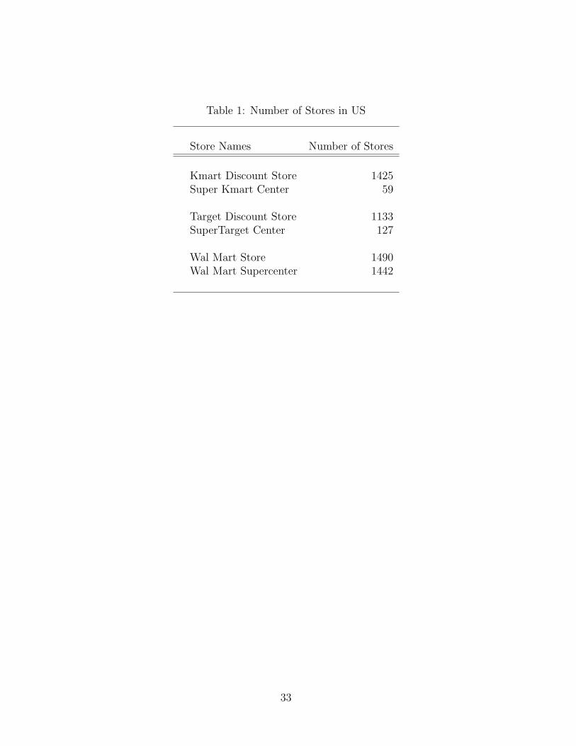
Table 1: Number of Stores in US

Store Names Number of Stores

Kmart Discount Store 1425Super Kmart Center 59

Target Discount Store 1133SuperTarget Center 127

Wal Mart Store 1490Wal Mart Supercenter 1442

33

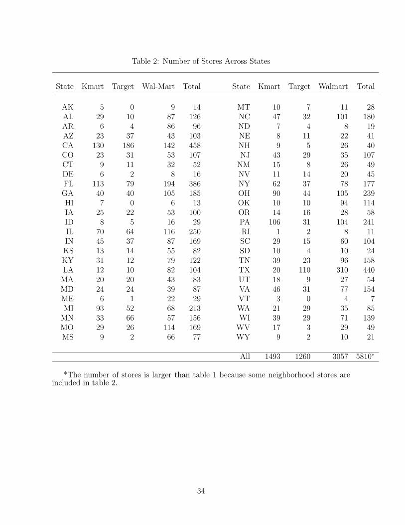
Table 2: Number of Stores Across States

State Kmart Target Wal-Mart Total State Kmart Target Walmart Total

AK 5 0 9 14 MT 10 7 11 28AL 29 10 87 126 NC 47 32 101 180AR 6 4 86 96 ND 7 4 8 19AZ 23 37 43 103 NE 8 11 22 41CA 130 186 142 458 NH 9 5 26 40CO 23 31 53 107 NJ 43 29 35 107CT 9 11 32 52 NM 15 8 26 49DE 6 2 8 16 NV 11 14 20 45FL 113 79 194 386 NY 62 37 78 177GA 40 40 105 185 OH 90 44 105 239HI 7 0 6 13 OK 10 10 94 114IA 25 22 53 100 OR 14 16 28 58ID 8 5 16 29 PA 106 31 104 241IL 70 64 116 250 RI 1 2 8 11IN 45 37 87 169 SC 29 15 60 104KS 13 14 55 82 SD 10 4 10 24KY 31 12 79 122 TN 39 23 96 158LA 12 10 82 104 TX 20 110 310 440MA 20 20 43 83 UT 18 9 27 54MD 24 24 39 87 VA 46 31 77 154ME 6 1 22 29 VT 3 0 4 7MI 93 52 68 213 WA 21 29 35 85

MN 33 66 57 156 WI 39 29 71 139MO 29 26 114 169 WV 17 3 29 49MS 9 2 66 77 WY 9 2 10 21

All 1493 1260 3057 5810∗

*The number of stores is larger than table 1 because some neighborhood stores areincluded in table 2.

34

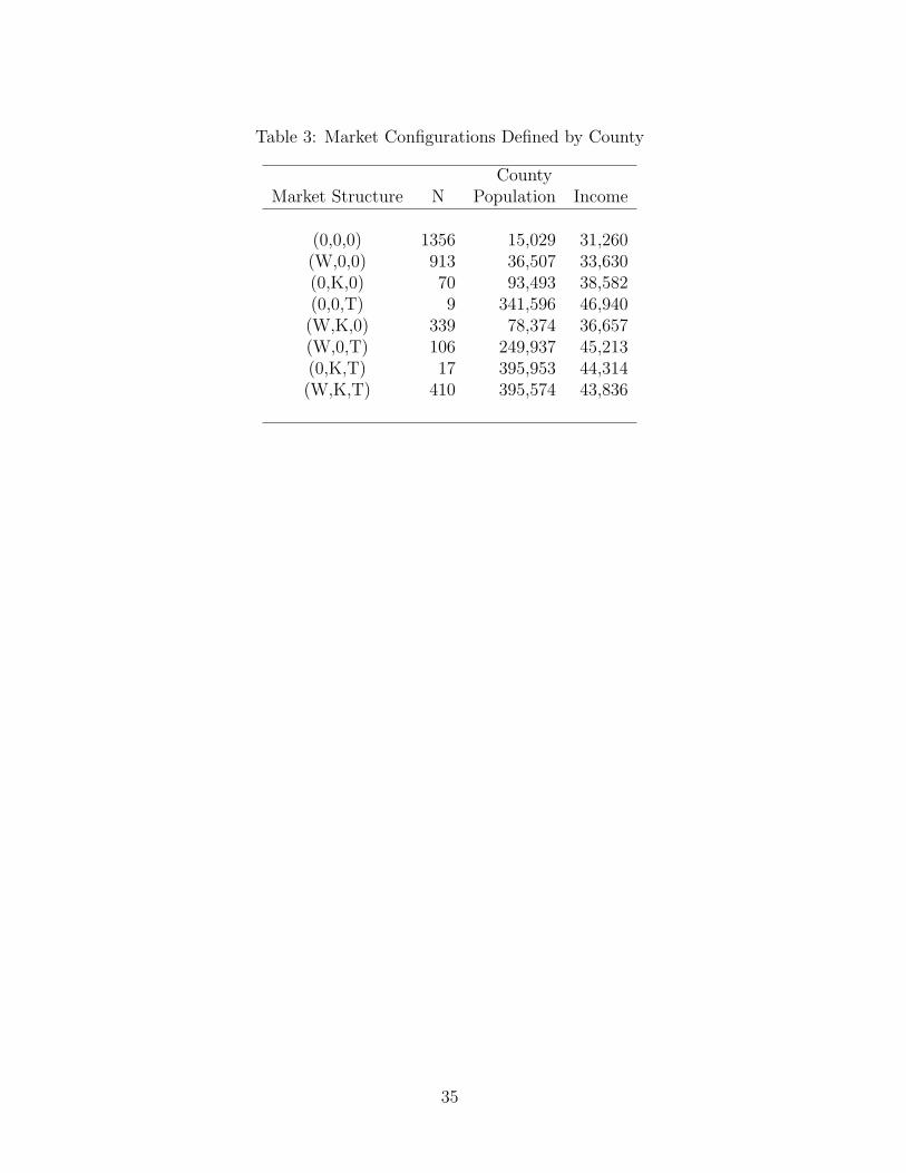
Table 3: Market Configurations Defined by County

CountyMarket Structure N Population Income

(0,0,0) 1356 15,029 31,260(W,0,0) 913 36,507 33,630(0,K,0) 70 93,493 38,582(0,0,T) 9 341,596 46,940(W,K,0) 339 78,374 36,657(W,0,T) 106 249,937 45,213(0,K,T) 17 395,953 44,314(W,K,T) 410 395,574 43,836

35

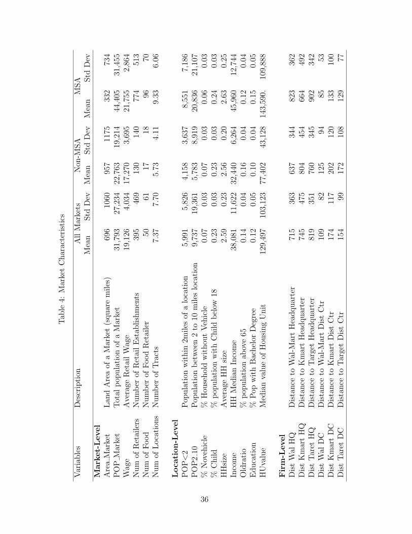
Tab

le4:

Mar

ket

Char

acte

rist

ics

Var

iable

sD

escr

iption

All

Mar

kets

Non

-MSA

MSA

Mea

nStd

Dev

Mea

nStd

Dev

Mea

nStd

Dev

Mark

et-

Level

Are

aM

arke

tLan

dA

rea

ofa

Mar

ket

(squar

em

iles

)69

610

6095

711

7533

273

4P

OP

Mar

ket

Tot

alpop

ula

tion

ofa

Mar

ket

31,7

9327

,234

22,7

6319

,214

44,4

0531

,455

Wag

eA

vera

geR

etai

lW

age

19,1

264,

034

17,2

703,

695

21,7

552,

864

Num

ofR

etai

lers

Num

ber

ofR

etai

lE

stab

lish

men

ts39

546

913

014

077

451

3N

um

ofFood

Num

ber

ofFood

Ret

aile

r50

6117

1896

70N

um

ofLoca

tion

sN

um

ber

ofTra

cts

7.37

7.70

5.73

4.11

9.33

6.06

Loca

tion-L

evel

PO

P<

2Pop

ula

tion

wit

hin

2miles

ofa

loca

tion

5,99

15,

826

4,15

83,

637

8,55

17,

186

PO

P2

10Pop

ula

tion

bet

wee

n2

to10

miles

loca

tion

9,73

719

,361

5,78

38,

919

20,8

3621

,107

%N

oveh

icle

%H

ouse

hol

dw

ithou

tVeh

icle

0.07

0.03

0.07

0.03

0.06

0.03

%C

hild

%pop

ula

tion

wit

hC

hild

bel

ow18

0.23

0.03

0.23

0.03

0.24

0.03

HH

size

Ave

rage

HH

size

2.59

0.23

2.56

0.20

2.63

0.25

Inco

me

HH

Med

ian

Inco

me

38,0

8111

,622

32,4

406,

264

45,9

6012

,744

Old

rati

o%

pop

ula

tion

abov

e65

0.14

0.04

0.16

0.04

0.12

0.04

Educa

tion

%Pop

wit

hB

achel

orD

egre

e0.

120.

050.

100.

040.

150.

05H

Uva

lue

Med

ian

valu

eof

Hou

sing

Unit

129,

497

103,

123

77,4

0243

,128

143,

590.

109,

888

Fir

m-L

evel

Dis

tW

alH

QD

ista

nce

toW

al-M

art

Hea

dquar

ter

715

363

637

344

823

362

Dis

tK

mar

tH

QD

ista

nce

toK

mar

tH

eadquar

ter

745

475

804

454

664

492

Dis

tTar

etH

QD

ista

nce

toTar

get

Hea

dquar

ter

819

351

760

345

902

342

Dis

tW

alD

CD

ista

nce

toW

al-M

art

Dis

tC

tr10

982

125

9485

53D

ist

Km

art

DC

Dis

tance

toK

mar

tD

ist

Ctr

174

117

202

120

133

100

Dis

tTar

etD

CD

ista

nce

toTar

get

Dis

tC

tr15

499

172

108

129

77

36

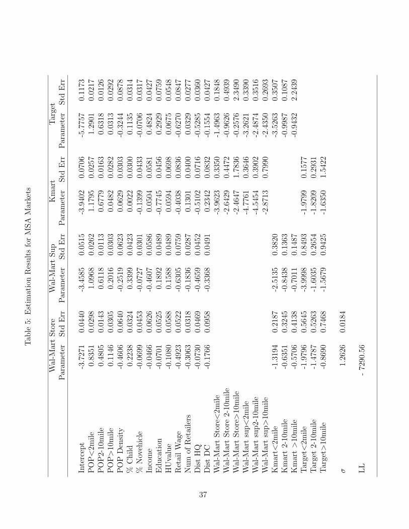
Tab

le5:

Est

imat

ion

Res

ult

sfo

rM

SA

Mar

kets

Wal

-Mar

tSto

reW

al-M

art

Sup

Km

art

Tar

get

Par

amet

erStd

Err

Par

amet

erStd

Err

Par

amet

erStd

Err

Par

amet

erStd

Err

Inte

rcep

t-3

.727

10.

0440

-3.4

585

0.05

15-3

.940

20.

0706

-5.7

757

0.11

73P

OP

<2m

ile

0.83

510.

0298

1.09

680.

0262

1.17

950.

0257

1.29

010.

0217

PO

P2-

10m

ile

0.48

050.

0143

0.61

180.

0113

0.67

790.

0163

0.63

180.

0126

PO

P>

10m

ile

0.11

460.

0305

0.20

160.

0303

0.04

820.

0282

0.03

130.

0292

PO

PD

ensi

ty-0

.460

60.

0640

-0.2

519

0.06

230.

0629

0.03

03-0

.324

40.

0878

%C

hild

0.22

380.

0324

0.33

990.

0423

0.00

220.

0300

0.11

350.

0314

%N

oveh

icle

-0.0

699

0.04

53-0

.072

70.

0301

-0.1

399

0.04

33-0

.070

60.

0317

Inco

me

-0.0

466

0.06

26-0

.460

70.

0586

0.05

040.

0581

0.48

240.

0427

Educa

tion

-0.0

701

0.05

250.

1892

0.04

89-0

.774

50.

0456

0.29

290.

0759

HU

valu

e-0

.108

00.

0588

0.15

880.

0489

0.05

940.

0698

0.06

750.

0548

Ret

ailW

age

-0.4

923

0.05

22-0

.630

50.

0759

-0.4

038

0.08

36-0

.627

00.

0847

Num

ofR

etai

lers

-0.3

063

0.03

18-0

.183

60.

0287

0.13

010.

0400

0.03

290.

0277

Dis

tH

Q-0

.073

00.

0469

-0.4

659

0.04

52-0

.510

20.

0716

-0.5

285

0.03

60D

ist

DC

-0.1

766

0.09

58-0

.336

80.

0491

0.23

420.

0832

-0.1

554

0.04

27W

al-M

art

Sto

re<

2mile

-3.9

623

0.33

50-1

.496

30.

1848

Wal

-Mar

tSto

re2-

10m

ile

-2.6

429

0.44

72-0

.962

60.

4939

Wal

-Mar

tSto

re>

10m

ile

-2.4

647

1.78

36-0

.257

62.

3490

Wal

-Mar

tsu

p<

2mile

-4.7

761

0.36

46-3

.262

10.

3390

Wal

-Mar

tsu

p2-

10m

ile

-4.5

454

0.39

02-2

.487

40.

3516

Wal

-Mar

tsu

p>

10m

ile

-2.8

713

0.79

90-2

.435

00.

2693

Km

art<

2mile

-1.3

194

0.21

87-2

.513

50.

3820

-3.5

263

0.35

07K

mar

t2-

10m

ile

-0.6

351

0.32

45-0

.843

80.

1363

-0.9

987

0.10

87K

mar

t>

10m

ile

-0.5

706

0.41

38-0

.701

10.

1487

-0.9

432

2.24

39Tar

get<

2mile

-1.9

796

0.56

45-3

.999

80.

8493

-1.9

799

0.15

77Tar

get

2-10

mile

-1.4

787

0.52

63-1

.603

50.

2654

-1.8

209

0.29

31Tar

get>

10m

ile

-0.8

690

0.74

68-1

.567

90.

9425

-1.6

350

1.54

22

σ1.

2626

0.01

84

LL

-72

90.5

6

37

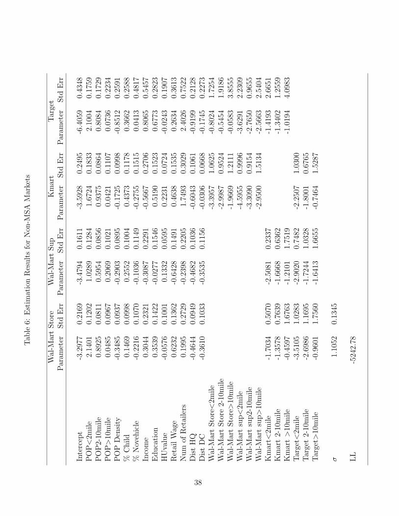
Tab

le6:

Est

imat

ion

Res

ult

sfo

rN

on-M

SA

Mar

kets

Wal

-Mar

tSto

reW

al-M

art

Sup

Km

art

Tar

get

Par

amet

erStd

Err

Par

amet

erStd

Err

Par

amet

erStd

Err

Par

amet

erStd

Err

Inte

rcep

t-3

.297

70.

2169

-3.4

794

0.16

11-3

.592

80.

2495

-6.4

059

0.43

48P

OP

<2m

ile

2.14

010.

1202

1.02

890.

1284

1.67

240.

1833

2.10

040.

1759

PO

P2-

10m

ile

0.89

250.

0811

0.59

540.

0856

0.93

750.

0864

0.80

840.

1729

PO

P>

10m

ile

0.04

850.

0967

0.20

690.

1021

0.04

210.

1107

0.07

360.

2234

PO

PD

ensi

ty-0

.348

50.

0937

-0.2

903

0.08

95-0

.172

50.

0998

-0.8

512

0.25

91%

Child

0.14

690.

0998

0.25

520.

1004

0.43

730.

1178

0.36

620.

2588

%N

oveh

icle

-0.2

216

0.10

70-0

.103

60.

1149

-0.2

755

0.15

150.

0413

0.48

17In

com

e0.

3044

0.23

21-0

.308

70.

2291

-0.5

667

0.27

060.

8065

0.54

57E

duca

tion

0.35

390.

1422

-0.0

277

0.15

460.

5190

0.15

230.

6773

0.28

23H

Uva

lue

-0.0

576

0.10

010.

1332

0.05

950.

2231

0.07

24-0

.024

30.

1907

Ret

ailW

age

0.62

320.

1362

-0.6

428

0.14

910.

4638

0.15

350.

2634

0.36

13N

um

ofR

etai

lers

0.19

950.

2729

-0.2

398

0.22

051.

7493

0.30

292.

4026

0.75

22D

ist

HQ

-0.4

644

0.09

49-0

.468

20.

1036

-0.6

043

0.10

61-0

.919

90.

2128

Dis

tD

C-0

.361

00.

1033

-0.3

535

0.11

56-0

.030

60.

0668

-0.1

745

0.22

73W

al-M

art

Sto

re<

2mile

-3.3

957

1.06

25-0

.802

41.

7254

Wal

-Mar

tSto

re2-

10m

ile

-2.9

987

0.95

24-0

.545

41.

9186

Wal

-Mar

tSto

re>

10m

ile

-1.9

669

1.21

11-0

.058

33.

8555

Wal

-Mar

tsu

p<

2mile

-4.5

955

0.99

96-3

.629

12.

2309

Wal

-Mar

tsu

p2-

10m

ile

-3.3

090

0.91

54-2

.765

00.

9655

Wal

-Mar

tsu

p>

10m

ile

-2.9

500

1.51

34-2

.566

32.

5404

Km

art<

2mile

-1.7

034

0.50

70-2

.508

10.

2337

-1.4

193

2.66

51K

mar

t2-

10m

ile

-1.3

578

0.76

39-1

.666

80.

6362

-1.3

402

1.25

59K

mar

t>

10m

ile

-0.4

597

1.67

63-1

.210

11.

7519

-1.0

194

4.09

83Tar

get<

2mile

-3.5

105

1.02

83-2

.902

00.

7482

-2.2

507

1.03

00Tar

get

2-10

mile

-2.6

986

1.16

95-1

.724

41.

0328

-1.8

001

0.67

65Tar

get>

10m

ile

-0.9

601

1.75

60-1

.641

31.

6655

-0.7

464

1.52

87

σ1.

1052

0.13

45

LL

-524

2.78

38

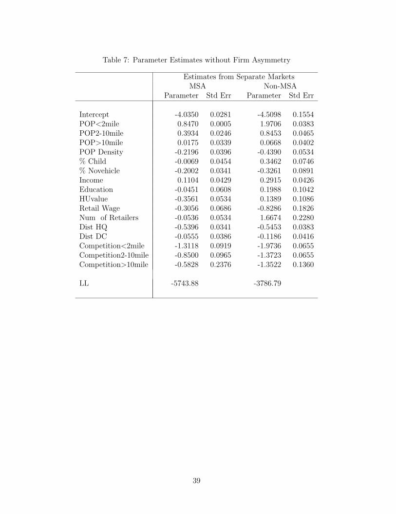
Table 7: Parameter Estimates without Firm Asymmetry

Estimates from Separate MarketsMSA Non-MSA

Parameter Std Err Parameter Std Err

Intercept -4.0350 0.0281 -4.5098 0.1554POP<2mile 0.8470 0.0005 1.9706 0.0383POP2-10mile 0.3934 0.0246 0.8453 0.0465POP>10mile 0.0175 0.0339 0.0668 0.0402POP Density -0.2196 0.0396 -0.4390 0.0534% Child -0.0069 0.0454 0.3462 0.0746% Novehicle -0.2002 0.0341 -0.3261 0.0891Income 0.1104 0.0429 0.2915 0.0426Education -0.0451 0.0608 0.1988 0.1042HUvalue -0.3561 0.0534 0.1389 0.1086Retail Wage -0.3056 0.0686 -0.8286 0.1826Num of Retailers -0.0536 0.0534 1.6674 0.2280Dist HQ -0.5396 0.0341 -0.5453 0.0383Dist DC -0.0555 0.0386 -0.1186 0.0416Competition<2mile -1.3118 0.0919 -1.9736 0.0655Competition2-10mile -0.8500 0.0965 -1.3723 0.0655Competition>10mile -0.5828 0.2376 -1.3522 0.1360

LL -5743.88 -3786.79

39

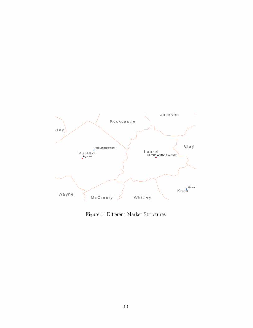
Wal Mart Store

Wal Mart Supercenter

Wal Mart SupercenterBig KmartBig Kmart

P u l a s k iP u l a s k i L a u r e lL a u r e l

K n o xK n o x

J a c k s o nJ a c k s o n

C l a yC l a y

L i n c o l nL i n c o l n

W h i t l e yW h i t l e yW a y n eW a y n e

R o c k c a s t l eR o c k c a s t l e

M c C r e a r yM c C r e a r y

C a s e yC a s e y

O w s l e yO w s l e y

L e eL e eG a r r a r dG a r r a r d

B e l lB e l l

M a d i s o nM a d i s o n

Figure 1: Different Market Structures

40

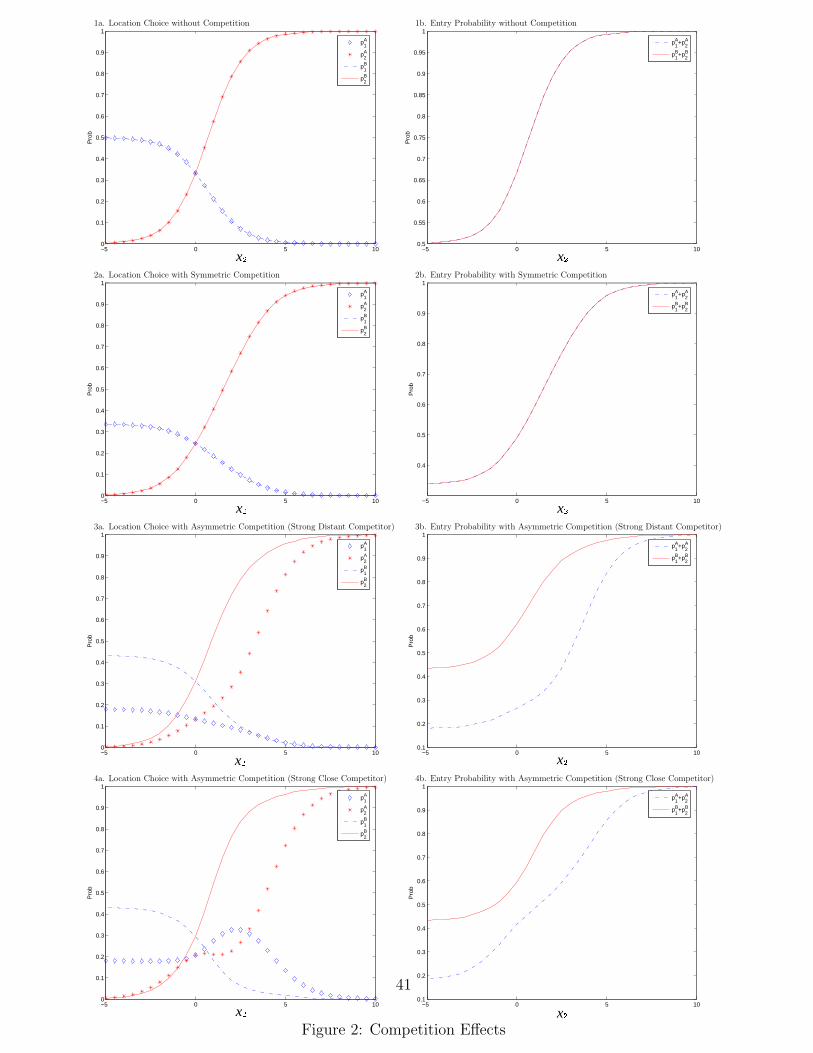
−5 0 5 100

0.1

0.2

0.3

0.4

0.5

0.6

0.7

0.8

0.9

1

Pro

b

p1A

p2A

p1B

p2B

x

1a. Location Choice without Competition

−5 0 5 100.5

0.55

0.6

0.65

0.7

0.75

0.8

0.85

0.9

0.95

1

Pro

b

p1A+p

2A

p1B+p

2B

x

1b. Entry Probability without Competition

−5 0 5 100

0.1

0.2

0.3

0.4

0.5

0.6

0.7

0.8

0.9

1

Pro

b

p1A

p2A

p1B

p2B

x

2a. Location Choice with Symmetric Competition

−5 0 5 10

0.4

0.5

0.6

0.7

0.8

0.9

1

Pro

b

p1A+p

2A

p1B+p

2B

x

2b. Entry Probability with Symmetric Competition

−5 0 5 100

0.1

0.2

0.3

0.4

0.5

0.6

0.7

0.8

0.9

1

Pro

b

p1A

p2A

p1B

p2B

x

3a. Location Choice with Asymmetric Competition (Strong Distant Competitor)

−5 0 5 100.1

0.2

0.3

0.4

0.5

0.6

0.7

0.8

0.9

1

Pro

b

p1A+p

2A

p1B+p

2B

x

3b. Entry Probability with Asymmetric Competition (Strong Distant Competitor)

−5 0 5 100

0.1

0.2

0.3

0.4

0.5

0.6

0.7

0.8

0.9

1

Pro

b

p1A

p2A

p1B

p2B

x

4a. Location Choice with Asymmetric Competition (Strong Close Competitor)

−5 0 5 100.1

0.2

0.3

0.4

0.5

0.6

0.7

0.8

0.9

1

Pro

b

p1A+p

2A

p1B+p

2B

x

4b. Entry Probability with Asymmetric Competition (Strong Close Competitor)

Figure 2: Competition Effects

41

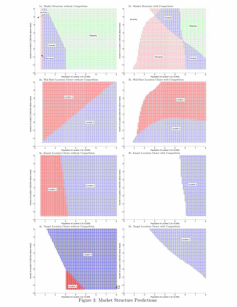
0 1 2 3 4 5 6 7 8−3

−2

−1

0

1

2

3

4

5

Population of Location 2 (in 10,000)

Inco

me

of L

ocat

ion

2 (S

td D

ev a

bove

mea

n)

No Entry

Monopoly

Duopoly

Oligopoly

1a. Market Structure without Competition

0 1 2 3 4 5 6 7 8−3

−2

−1

0

1

2

3

4

5

Population of Location 2 (in 10,000)

Inco

me

of L

ocat

ion

2 (S

td D

ev a

bove

mea

n)

No Entry

MonopolyDuopoly

Oligopoly

Duopoly

Oligopoly

1b. Market Structure with Competition

0 1 2 3 4 5 6 7 8−3

−2

−1

0

1

2

3

4

5

Population of Location 2 (in 10,000)

Inco

me

of L

ocat

ion

2 (S

td D

ev a

bove

mea

n)

Location 2

Location 1

2a. Wal-Mart Location Choice without Competition

0 1 2 3 4 5 6 7 8−3

−2

−1

0

1

2

3

4

5

Population of Location 2 (in 10,000)

Inco

me

of L

ocat

ion

2(S

td D

ev a

bove

mea

n)

Location 2

Location 1

2b. Wal-Mart Location Choice with Competition

0 1 2 3 4 5 6 7 8−3

−2

−1

0

1

2

3

4

5

Population of Location 2 (in 10,000)

Inco

me

of L

ocat

ion

2 (S

td D

ev a

bove

mea

n)

Location 2

Location 1

3a. Kmart Location Choice without Competition

0 1 2 3 4 5 6 7 8−3

−2

−1

0

1

2

3

4

5

Population of Location 2 (in 10,000)

Inco

me

of L

ocat

ion

2 (S

td D

ev a

bove

mea

n)

Location 2

3b. Kmart Location Choice with Competition

0 1 2 3 4 5 6 7 8−3

−2

−1

0

1

2

3

4

5

Population of Location 2 (in 10,000)

Inco

me

of L

ocat

ion

2 (S

td D

ev a

bove

mea

n)

Location 2

Location 1

4a. Target Location Choice without Competition

0 1 2 3 4 5 6 7 8−3

−2

−1

0

1

2

3

4

5

Population of Location 2 (in 10,000)

Inco

me

of L

ocat

ion

2 (S

td D

ev a

bove

mea

n)

Location 2

4b. Target Location Choice with Competition

Figure 3: Market Structure Predictions

42

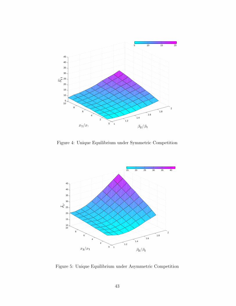
11.2

1.41.6

1.82

0

2

4

6

8

105

10

15

20

25

30

35

40

45

5 10 15 20

Figure 4: Unique Equilibrium under Symmetric Competition

11.2

1.41.6

1.82

0

2

4

6

8

1010

15

20

25

30

35

40

45

15 20 25 30 35 40

Figure 5: Unique Equilibrium under Asymmetric Competition

43