SPATIAL MEASUREMENT OF RESIDENTIAL SEGREGATION

Flávia F. Feitosa1, Gilberto Câmara1, Antônio M. V. Monteiro1, Thomas Koschitzki2 and Marcelino P. S. Silva1,3

1INPE - Instituto Nacional de Pesquisas Espaciais. Av. dos Astronautas, 1758, São José dos Campos (SP), Brazil, 12227-001. {flavia, gilberto, miguel, mpss}@dpi.inpe.br; 2Martin-Luther Universität Halle-Wittenberg. Institut für Geographie. Von-Seckendorff-Platz 4, Halle (Saale), 06120, Germany. koschitzki@geographie.uni-halle.de; 3UERN - Universidade do Estado do Rio Grande do Norte, BR 110, Km 48, 59610-090, Mossoró, RN, Brazil.

Abstract: Segregation measures are useful tools for the analysis of patterns, causes and effects of residential segregation. However, most of empirical segregation studies have employed nonspatial and global measures. In other words, the measures so far applied are unable to consider the spatial arrangement of population and to show how much each areal unit contributes to the segregation degree of the whole city. This paper presents an alternative to overcome the mentioned shortcomings. Specifically, we extended existing segregation indices to enable the use of spatial information in their formulations, and we decomposed the extended indices to generate new local measures of segregation. Finally, the proposed measures were evaluated using an artificial dataset as well as a case study of residential segregation in São José dos Campos (SP, Brazil).

Key words: residential segregation; spatial segregation measures; São José dos Campos (SP, Brazil).

1. INTRODUCTION

Residential segregation is the degree of spatial proximity between families belonging to the same social group (Sabatini et al., 2001). In Latin America, where the attributes that characterize segregation are mainly socioeconomic, there are several evidences that residential segregation causes the intensification of poverty and social problems in many areas (Sabatini et al., 2001; Rodríguez, 2001; Torres, 2004; Luco and Rodríguez,

60

2003). For this reason, the theme has received increasing attention in public policy literature.

In spite of the emphasis given to the issue, there are few Latin-American studies focused on the measurement of residential segregation. The existing studies rely on nonspatial measures such as the dissimilarity index (Sabatini et al., 2001; Torres, 2004; Telles, 1992) or variance-based indices (Rodríguez, 2001). These measures are not able to distinguish different spatial arrangements among population groups, which is an essential aspect in segregation studies.

Another drawback concerning the use of traditional segregation measures is that they are global measures. In other words, they express the segregation degree of the city as a whole. However, the degree of residential segregation is a nonstationary process, which varies along the city (Wong, 2003b). Thus, the measurement of segregation requires also local indices, able to depict how much each areal unit contributes to the composition of the global index.

This paper presents an alternative to overcome the limitations mentioned above. Specifically, we (a) extend some of the existing segregation indices to enable the use of geographical information in their formulations; (b) propose new local indices of segregation, obtained by decomposing the extended indices; and (c) evaluate the developed measures using an artificial dataset and a case study of residential segregation in São José dos Campos (SP, Brazil). First, we present a brief review of previous studies on segregation measurement.

2. MEASURES OF RESIDENTIAL SEGREGATION

The first studies focused on the measurement of segregation date from the late 1940s and the beginning of 1950s, when several indices were proposed and discussed in the United States. The most popular index of this first generation of measures is the dissimilarity index D, idealized by Duncan and Duncan (1955). The dissimilarity index, still used by many researchers, represents the proportion of population from a specific social group that would have to relocate within the city so that each area of it would have the same social composition of the city as a whole. The index ranges from 0 to 1 (maximum segregation) and is defined as

n

inI

i m

im

NN

NN

D −= ∑=12

1 , (1)

where Nim and Nin are the population of group m and n, respectively, in areal unit i, while Nm and Nn are the total population of groups m and n in the city.

61

Besides the dissimilarity index, other indices were developed, like the P* exposure index (Bell, 1954), the Gini index (Cowell, 1977), the Information Theory index (Bell, 1954), and the Atkinson index (Atkinson, 1970).

However, all indices proposed in this phase have been limited to measure segregation between two population groups. This restriction reflects the social concerns for which such indices were developed: the Black and White residential segregation during the civil rights era, from the 1950s through the 1970s (Reardon and Firebaugh, 2002).

In the 1970s, segregation studies started to became increasingly focused on multi-group issues, like the segregation among social classes or among White, Blacks and Hispanics. To meet these new needs, a second generation of segregation indices started to be proposed (Reardon and Firebaugh, 2002; Morgan,1975; Sakoda, 1981; Jargowsky, 1996). These new multi-group measures were usually generalized versions of the existent two-group measures.

Nevertheless, the multi-group measures still keep the most criticized limitation of the first indices: the incapability to depict the spatial arrangement of population among areal units (Rodríguez, 2001; Reardon and Firebaugh, 2002). Hence, several studies started to focus on the development of spatial measures of segregation (Morgan, 1981; White, 1983; Wong, 2003a; Reardon and O’Sullivan, 2004).

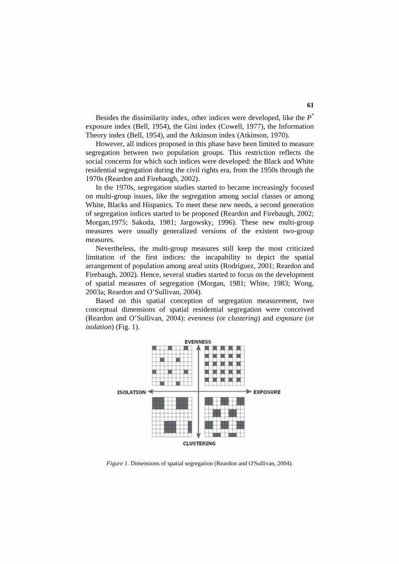
Based on this spatial conception of segregation measurement, two conceptual dimensions of spatial residential segregation were conceived (Reardon and O’Sullivan, 2004): evenness (or clustering) and exposure (or isolation) (Fig. 1).

Figure 1. Dimensions of spatial segregation (Reardon and O'Sullivan, 2004).

62

The dimension evenness or clustering refers to the balance of the distribution of population groups and it is independent of the population composition of the city as a whole (Reardon and O’Sullivan, 2004). Exposure or isolation refers to the chance of having members from different groups (or the same group, if we consider isolation) living side-by-side. Exposure depends on the overall population composition of the city (Reardon and O’Sullivan, 2004).

Although some spatial indices have been already developed, most of empirical studies still rely on nonspatial indices. This happens because spatial measures always require the extraction of geographical information and are more difficult to compute than nonspatial measures.

3. EXTENDING TRADITIONAL NONSPATIAL MEASURES

In order to obtain segregation measures able to distinguish different spatial arrangements among population groups, three existing nonspatial indices were extended: the generalized dissimilarity index D(m) (Morgan, 1975; Sakoda, 1981), the exposure index P* (Bell, 1954) and the residential segregation index RSI (Jargowsky, 1996; Rodríguez, 2001). The indices D(m) and RSI represent the dimension evenness/clustering while the index P* measures the dimension exposure/isolation.

In spite of the easy interpretation of the indices D(m) and P*, some scholars consider them unsuitable to socioeconomic segregation studies (Jargowsky, 1996; Rodríguez, 2001). They argue that these indices are unable to use the original distribution of continuous variables (e.g., income of householders), and therefore require arbitrary cutoff points for the establishment of population groups. For this reason, the residential segregation index RSI was also extended. The RSI is more appropriate for segregation studies based on continuous variables because it is a variance-based measure and avoids the need of grouping.

Nevertheless, most of empirical studies are based on aggregate data, which variables are not provided in their original distribution, but in artificially-built intervals (e.g., householders with income less than 2 minimum wages, householders with income between 2 and 5 minimum wages, and so forth). Thus, the idea of population groups still remains in these studies, and the merit of RSI is reduced to its ability to order these groups. In other words, by means of the RSI, it is possible to consider that a group such as unemployed householders is closer to the group of householders with income less than 2 minimum wages than to the group of householders with income greater than 20 minimum wages.

63

In this study, we present a procedure of extending segregation indices based on approaches introduced by Wong (2003a) and Reardon and O’Sullivan (2004). These approaches cover analyses with different kinds of data – Wong with zones (population count) and Reardon and O´Sullivan with surfaces (population density) - and support the definition of “neighborhoods” where families interact. These neighborhoods - also called “local environment” (Reardon and O’Sullivan, 2004) - are established by proximity functions, chosen by the user according to the purposes of the study.

Like in Wong’s approach, we deal with population count data and the neighborhood population count of areal unit i for group m is defined as (Wong, 2003a)

(∑=

=I

iimim NdN

1

( ), (2)

where Nim is the population of the group m in areal unit i, and d(.) is the proximity function defining the neighborhood of i. The neighborhood population count in i is defined as the sum of the population of all areal units, where units are weighted by their proximity to i.

Following the same reasoning, we define the proportion of group m in the neighborhood of unit i ( imρ( ) as the ratio of the neighborhood population count of group m in areal unit i to the total neighborhood population count of i:

i

imim N

N(

(( =ρ . (3)

Based on the concept of neighborhood population count, the indices D(m), P* and RSI were modified to incorporate spatial information in their formulations. Our spatial versions of D(m) and P* are very similar to the indices proposed by Reardon and O’Sullivan (2004). In the latter case, however, the indices were developed for population density data, while the indices presented in this paper employ population count data.

The spatial version of the generalized dissimilarity index )(mD(

is defined as

mim

I

i

M

m

i

NINmD ρρ −=∑∑

= =

((

1 1 2)( , (4)

where

64

( )( m

M

mmI ρρ −= ∑

=

11

) . (5)

In Eq. (4) and (5), N is the total population of the city, Ni is the total population in area i, mρ is the proportion of group m in the city, and imρ( is the proportion of group m in the neighborhood of i. I represents the interaction index, a diversity measure of population (White, 1986). The index )(mD

( can be interpreted as a measure of how different the population

composition of all neighborhoods is, on average, from the population composition of the city as a whole (Reardon and O’Sullivan, 2004).

The spatial version of the exposure index of group m to group n ( *nm P(

) is defined as the average proportion of group n in the neighborhood of each member of group m (Reardon and O’Sullivan, 2004):

in

I

i m

imnm N

NP ρ((

∑=

=1

* . (6)

Equally, the spatial isolation index of group m can be defined as the spatial exposure of group m to itself:

im

I

i m

immm N

NP ρ((

∑=

=1

* . (7)

Considering a quantitative variable X, the third extended index – RSI – relies on the fact that the total variance of X in the city is the sum of the between-area variance and the intra-area variance of X. Therefore, the RSI is the proportion of the total variance of X (

2totalσ ) which is explained by the

between-area variance (2betweenσ ). In this paper, we propose a spatial version of

RSI ( ISR(

) defined as

1002

2

×=total

betweenISRσσ(

((. (8)

The variance of X between the different neighborhoods of the city is defined as:

( )N

XXNI

iii

between (

(((

(∑=

−= 1

22

2σ , (9)

65

where

N

XNX

I

iii

(

((( ∑

== 1 and ∑=

=I

iiNN

1

((. (10)(11)

In Eq. (9), (10) and (11), iN(

is the total neighborhood population count of i, iX

( is the average of X in the neighborhood of i, and X is the average of

X in the whole city. The total variance of X, considering the neighborhoods of the city, is

defined as

( )N

XXNM

mmm

total (

((

(∑=

−= 1

2

2σ , (12)

where

∑=

=I

iimm NN

1

((. (13)

In Eq. (12) and (13), imN(

is the neighborhood population of group m in unit i, mN

( is the total population count in unit i, and is the value of X for

group m. mX

4. LOCAL MEASURES OF SEGREGATION

All the indices presented until now are regarded as global measures, which summarize the degree of residential segregation of the entire city. However, segregation is a process that varies along the city and the exclusive use of global measures can imply in the loss of useful information. Therefore, besides global measures, it is also important to rely on local indices that can be geographically displayed as maps and enable further analyses in a different level (Wong, 2003b).

In this paper, we propose two new local indices of segregation, obtained by decomposing the global indices )(mD

( and *P

(. These local indices show

how much each unit and its neighborhood contribute to the global segregation measure of a city. The local version of )(mD

( - )(md

(- is defined

as

66

mim

M

m

i

NIN

md ρρ −= ∑=

((

1 2)( . (14)

Likewise, the local version of the exposure index of group m to group n ( nm p( ) is defined as

inm

imnm N

Np ρ(( =* . (15)

5. EXPERIMENTS USING ARTIFICIAL DATA SETS

For the purpose of comparing the nonspatial and spatial measures, three artificial datasets were created (Fig. 2).

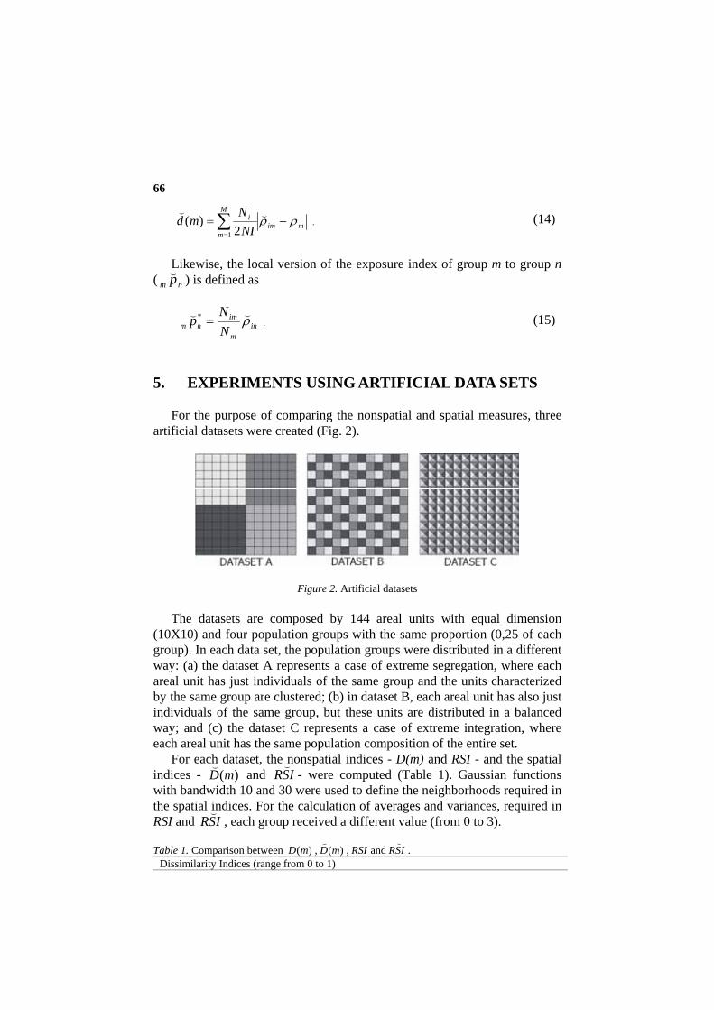
Figure 2. Artificial datasets

The datasets are composed by 144 areal units with equal dimension (10X10) and four population groups with the same proportion (0,25 of each group). In each data set, the population groups were distributed in a different way: (a) the dataset A represents a case of extreme segregation, where each areal unit has just individuals of the same group and the units characterized by the same group are clustered; (b) in dataset B, each areal unit has also just individuals of the same group, but these units are distributed in a balanced way; and (c) the dataset C represents a case of extreme integration, where each areal unit has the same population composition of the entire set.

For each dataset, the nonspatial indices - D(m) and RSI - and the spatial indices - )(mD

( and ISR

(- were computed (Table 1). Gaussian functions

with bandwidth 10 and 30 were used to define the neighborhoods required in the spatial indices. For the calculation of averages and variances, required in RSI and ISR

(, each group received a different value (from 0 to 3).

Table 1. Comparison between ,)(mD )(mD(

, andRSI ISR(

. Dissimilarity Indices (range from 0 to 1)

67

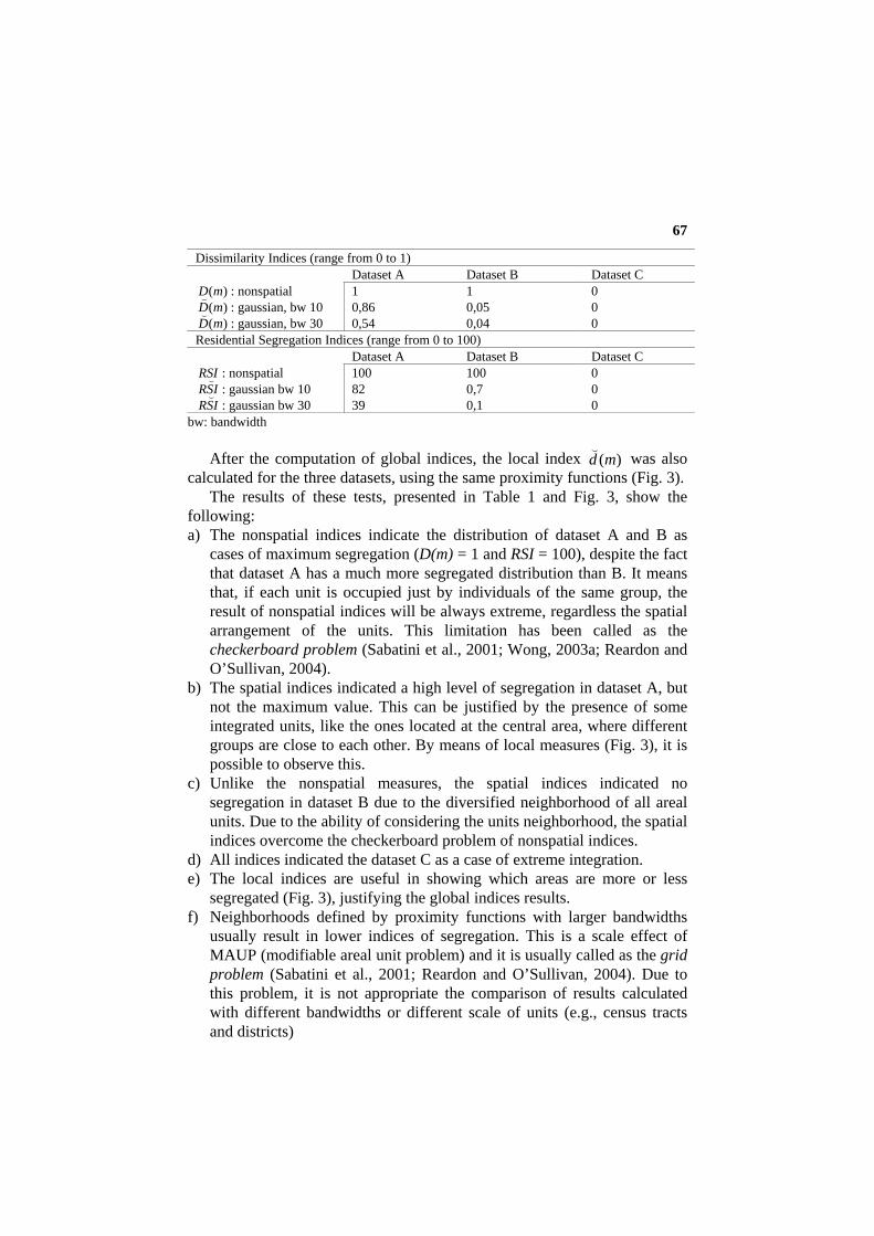
Dissimilarity Indices (range from 0 to 1) Dataset A Dataset B Dataset C

)(mD : nonspatial 1 1 0 )(mD

(: gaussian, bw 10 0,86 0,05 0

)(mD(

: gaussian, bw 30 0,54 0,04 0 Residential Segregation Indices (range from 0 to 100) Dataset A Dataset B Dataset C RSI : nonspatial 100 100 0

ISR(

: gaussian bw 10 82 0,7 0 ISR(

: gaussian bw 30 39 0,1 0 bw: bandwidth

After the computation of global indices, the local index )(md

( was also

calculated for the three datasets, using the same proximity functions (Fig. 3). The results of these tests, presented in Table 1 and Fig. 3, show the

following: a) The nonspatial indices indicate the distribution of dataset A and B as

cases of maximum segregation (D(m) = 1 and RSI = 100), despite the fact that dataset A has a much more segregated distribution than B. It means that, if each unit is occupied just by individuals of the same group, the result of nonspatial indices will be always extreme, regardless the spatial arrangement of the units. This limitation has been called as the checkerboard problem (Sabatini et al., 2001; Wong, 2003a; Reardon and O’Sullivan, 2004).

b) The spatial indices indicated a high level of segregation in dataset A, but not the maximum value. This can be justified by the presence of some integrated units, like the ones located at the central area, where different groups are close to each other. By means of local measures (Fig. 3), it is possible to observe this.

c) Unlike the nonspatial measures, the spatial indices indicated no segregation in dataset B due to the diversified neighborhood of all areal units. Due to the ability of considering the units neighborhood, the spatial indices overcome the checkerboard problem of nonspatial indices.

d) All indices indicated the dataset C as a case of extreme integration. e) The local indices are useful in showing which areas are more or less

segregated (Fig. 3), justifying the global indices results. f) Neighborhoods defined by proximity functions with larger bandwidths

usually result in lower indices of segregation. This is a scale effect of MAUP (modifiable areal unit problem) and it is usually called as the grid problem (Sabatini et al., 2001; Reardon and O’Sullivan, 2004). Due to this problem, it is not appropriate the comparison of results calculated with different bandwidths or different scale of units (e.g., census tracts and districts)

68

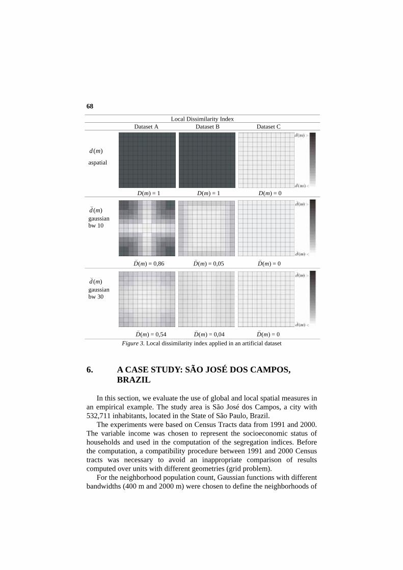
Local Dissimilarity Index Dataset A Dataset B Dataset C

)(md

aspatial

= 1 = 1 = 0 )(mD )(mD )(mD

)(md

(

gaussian bw 10

)(mD

(= 0,86 )(mD

(= 0,05 )(mD

(= 0

)(md

( gaussian bw 30

= 0,54 )(mD

()(mD

(= 0,04 )(mD

(= 0

Figure 3. Local dissimilarity index applied in an artificial dataset

6. A CASE STUDY: SÃO JOSÉ DOS CAMPOS, BRAZIL

In this section, we evaluate the use of global and local spatial measures in an empirical example. The study area is São José dos Campos, a city with 532,711 inhabitants, located in the State of São Paulo, Brazil.

The experiments were based on Census Tracts data from 1991 and 2000. The variable income was chosen to represent the socioeconomic status of households and used in the computation of the segregation indices. Before the computation, a compatibility procedure between 1991 and 2000 Census tracts was necessary to avoid an inappropriate comparison of results computed over units with different geometries (grid problem).

For the neighborhood population count, Gaussian functions with different bandwidths (400 m and 2000 m) were chosen to define the neighborhoods of

69

each areal unit and an application was developed to compute them. The selection of different bandwidths allows the examination of segregation on different scales, an issue which has been discussed in several studies (Sabatini et al., 2001; Rodríguez, 2001; Torres, 2004). According to Sabatini et al. (2001), both dimensions of segregation (evenness and exposure) can show different trends if we analyze them on different scales.

After the neighborhood population count of all units, the following indices were computed (Table 2): a) )(mD

(: Spatial dissimilarity index;

b) ISR(

: Spatial residential segregation index; c) : Spatial isolation index of householders with income greater than 20

minimum wages;

*2020 P(

d) *00 P(

: Spatial isolation index of unemployed householders; e) : Spatial exposure index of householders with income greater than 20

minimum wages to unemployed householders; *

*020 P(

f) 1020 P(

: Spatial exposure index of householders with income greater than 20 minimum wages to householders with income between 10 and 20 minimum wages;

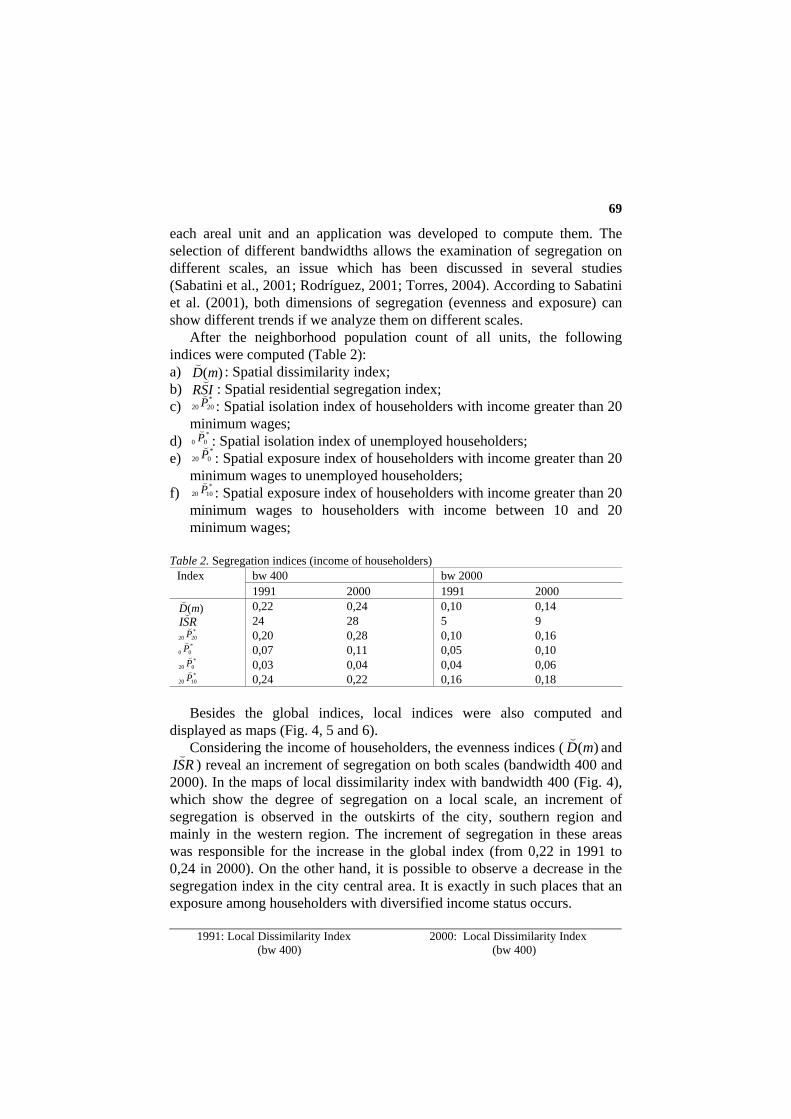
Table 2. Segregation indices (income of householders)

bw 400 bw 2000 Index 1991 2000 1991 2000

)(mD( 0,22 0,24 0,10 0,14

RSI(

24 28 5 9 *

2020 P(

0,20 0,28 0,10 0,16 *

00 P(

0,07 0,11 0,05 0,10 *

020 P(

0,03 0,04 0,04 0,06 *

1020 P(

0,24 0,22 0,16 0,18

Besides the global indices, local indices were also computed and displayed as maps (Fig. 4, 5 and 6).

Considering the income of householders, the evenness indices ( )(mD(

and RSI(

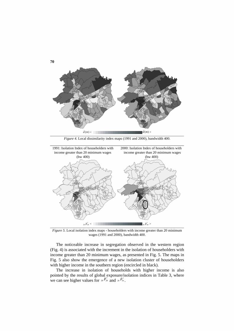
) reveal an increment of segregation on both scales (bandwidth 400 and 2000). In the maps of local dissimilarity index with bandwidth 400 (Fig. 4), which show the degree of segregation on a local scale, an increment of segregation is observed in the outskirts of the city, southern region and mainly in the western region. The increment of segregation in these areas was responsible for the increase in the global index (from 0,22 in 1991 to 0,24 in 2000). On the other hand, it is possible to observe a decrease in the segregation index in the city central area. It is exactly in such places that an exposure among householders with diversified income status occurs.

1991: Local Dissimilarity Index 2000: Local Dissimilarity Index (bw 400) (bw 400)

70

<)(md

( >)(md

(

Figure 4. Local dissimilarity index maps (1991 and 2000), bandwidth 400.

1991: Isolation Index of householders with 2000: Isolation Index of householders with income greater than 20 minimum wages income greater than 20 minimum wages (bw 400) (bw 400)

<*

2020 p( >*2020 p(

Figure 5. Local isolation index maps - householders with income greater than 20 minimum wages (1991 and 2000), bandwidth 400.

The noticeable increase in segregation observed in the western region (Fig. 4) is associated with the increment in the isolation of householders with income greater than 20 minimum wages, as presented in Fig. 5. The maps in Fig. 5 also show the emergence of a new isolation cluster of householders with higher income in the southern region (encircled in black).

The increase in isolation of households with higher income is also pointed by the results of global exposure/isolation indices in Table 3, where we can see higher values for

*2020 P(

and *1020 P(

.

71

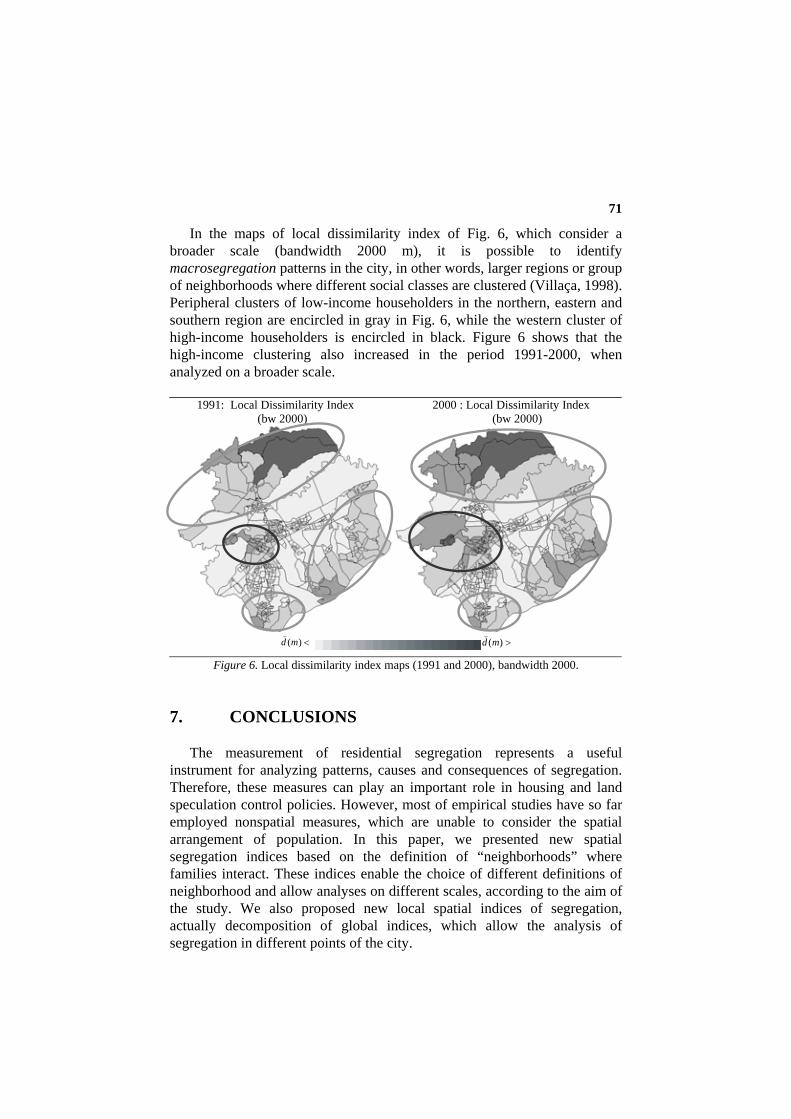
In the maps of local dissimilarity index of Fig. 6, which consider a broader scale (bandwidth 2000 m), it is possible to identify macrosegregation patterns in the city, in other words, larger regions or group of neighborhoods where different social classes are clustered (Villaça, 1998). Peripheral clusters of low-income householders in the northern, eastern and southern region are encircled in gray in Fig. 6, while the western cluster of high-income householders is encircled in black. Figure 6 shows that the high-income clustering also increased in the period 1991-2000, when analyzed on a broader scale.

1991: Local Dissimilarity Index 2000 : Local Dissimilarity Index (bw 2000) (bw 2000)

<)(md

(

>)(md(

Figure 6. Local dissimilarity index maps (1991 and 2000), bandwidth 2000.

7. CONCLUSIONS

The measurement of residential segregation represents a useful instrument for analyzing patterns, causes and consequences of segregation. Therefore, these measures can play an important role in housing and land speculation control policies. However, most of empirical studies have so far employed nonspatial measures, which are unable to consider the spatial arrangement of population. In this paper, we presented new spatial segregation indices based on the definition of “neighborhoods” where families interact. These indices enable the choice of different definitions of neighborhood and allow analyses on different scales, according to the aim of the study. We also proposed new local spatial indices of segregation, actually decomposition of global indices, which allow the analysis of segregation in different points of the city.

72

With the purpose of evaluating the developed measures, we applied them over an artificial dataset and in a real case study. In the latter, the use of evenness and isolation spatial measures, in their global and local versions, allowed complementary analyses about patterns of residential segregation in the city of São José dos Campos. The application of different bandwidths also revealed interesting aspects, indicating the degree of segregation on different scales: on a local scale it is possible to see details about the segregation degree in different areas, while on a broader scale it is possible to identify large regions where certain groups tend to concentrate (macrosegregation).

In the case of São José dos Campos, the indices )(mD(

and ISR(

presented very similar results concerning the segregation evolution from 1991 to 2000. In spite of these results, it is worthwhile remember that ISR

( is

more appropriate to socioeconomic studies than )(mD(

. Nevertheless, the exclusive use of ISR

(still presents two constraints: we cannot decompose it

to derive local measures, and it measures just the evenness dimension of segregation.

Another drawback, inherent to the application of all indices, is the absence of statistical procedures for assessing a threshold that determines whether a certain distribution is segregated or integrated. Although all the indices range from 0 to 1 (or from 0 to 100), the results depend on the scale and geometry of the units and, therefore, the absence of this threshold limits the indices application to comparative studies conducted for the same city.

ACKNOWLEDGEMENTS

The authors gratefully acknowledge the supports of CAPES and UERN as well as the reviews of Dr. Cláudia Almeida and Paulina Hoffmann.

REFERENCES

Atkinson, A. B., 1970, On the measures of inequality, Journal of Economic Theory. 2: 244-63.

Bell, W., 1954, A probability model for the measurement of ecological segregation, Social Forces. 32: 337-64.

Cowell, F. A., 1977, Measuring Inequality, Philip Allan, Oxford. Duncan, O. D., and Duncan, B., 1955, A methodological analysis of segregation indexes,

American Sociological Review. 20: 210-17. Luco, A., and Rodríguez, J., 2003, Segregación Residencial en Áreas Metropolitanas de

América Latina: Magnitud, Características, Evolución e Implicaciones de Política. Naciones Unidas, Santiago de Chile.

73

Jargowsky, P. A., 1996, Take the money and run: Economic segregation in U.S. metropolitan areas, American Journal of Sociology. 61: 984-99.

Morgan, B. S., 1975, The segregation of socioeconomic groups in urban areas: A comparative analysis. Urban Studies. 12: 47-60.

Morgan, B. S., 1981, A distance-decay interaction index to measure residential segregation, Demography. 18: 251-55.

Reardon, S. F., and Firebaugh, G., 2002, Measures of multigroup segregation, Sociological Methodology. 32: 33-67.

Reardon, S. F., and O´Sullivan, D., 2004, Measures of Spatial Segregation, Pennsylvania State University.

Rodríguez, J., 2001, Segregación Residencial Socioeconómica: Que És?, Cómo De Mide?, Que Está Pasando?, Importa?, CELADE/UNFPA, Santiago de Chile.

Sabatini, F., Cáceres, G., Cerdá, J., 2001, Segregación residencial en las principales ciudades chilenas: Tendencias de las tres últimas décadas y posibles cursos de acción, EURE (Santiago). 27: 21-42.

Sakoda, J., 1981, A generalized index of dissimilarity, Demography. 18: 245-50. Telles, E., 1992, Residential segregation by skin color in Brazil, American Sociological

Review. 57(2): 186-98. Torres, H., 2004, Segregação residencial e políticas públicas: São Paulo na década de 1990,

Revista Brasileira de Ciências Sociais. 54: 41-56. Villaça, F., 1998, Espaço Intra-Urbano no Brasil. Studio Nobel, São Paulo. White, M. J., 1983, The measurement of spatial segregation. American Journal of Sociology.

88: 1008-18. White, M. J., 1986, Segregation and diversity measures in population distribution, Population

Index. 52: 198-221. Wong, D. W. S., 2003a, Implementing spatial segregation measures in GIS, Computers,

Environment and Urban Systems. 27: 53-70. Wong, D. W. S., 2003b, Spatial decomposition of segregation indices: A framework toward

measuring segregation at multiple levels. Geographical Analysis. 35: 179-94.

74