Spherical Means and Distributions in Clifford Analysis

Spherical Means and Distributions inClifford Analysis

Fred Brackx, Richard Delanghe, and Frank Sommen

Abstract. This paper consists of two parts. In the first part we deal with spe-cific higher dimensional distributions within the framework of Clifford anal-ysis. These distributions are ”classical” in the sense that they were alreadyintroduced, albeit dispersed, in the literature on harmonic analysis and onClifford analysis. Amongst these classical distributions are the fundamentalsolutions of the natural powers of the Laplace and the Dirac operators, andthe integral kernel of the Hilbert transform. The strength of our approach isits unifying character.In the second part new higher dimensional distributions are introduced, gen-eralizing the distributions of part I. Crucial to this generalization is the useof so-called surface spherical monogenics. The whole picture thus obtainedoffers structural clarity and unity.

Introduction

The immediate cause of writing this paper was Delanghe’s paper [5] in which hestudies a higher dimensional analogue of the Principal Value distribution on thereal line. In that paper the integrated approach to all dimensions, offered by Clif-ford analysis, is fully exploited, as opposed to a traditional tensorial or cartesianapproach with a number of copies of one dimensional phenomena. We realizedthat this higher dimensional Principal Value distribution and the well known fun-damental solution of the Dirac operator are but two examples of vector valuedClifford distributions, out of an infinite collection of such kind of distributions,which moreover can be obtained by letting act the Dirac operator on a corre-sponding infinite set of classical real valued radial distributions. We also realizedthat by making use of the well known spherical means, which arise naturally byintroducing spherical co-ordinates, a simple, powerful and highly efficient tech-nique could be designed allowing us to carry out the explicit calculations on thereal line and exporting them to the original setting of Euclidean space. Finallywe realized that introducing generalized spherical means involving the so-called

Received by the editors November 26, 2002.

1991 Mathematics Subject Classification. Primary 30G35; Secondary 46F10.

Key words and phrases. distributions, spherical means, Clifford analysis.

2 F Brackx, R Delanghe, and F Sommen

spherical monogenics – the well known counterparts in Clifford analysis to thespherical harmonics of harmonic analysis – gave rise to much more general Clif-ford distributions, encompassing those from part I in the special case where thedegree of the spherical monogenic considered is zero.

The aim of this paper is twofold. From the scientific point of view we introducenew Clifford distributions generalizing and extending the existing ones in harmonicanalysis and Clifford analysis. From the didactic point of view our unifying ap-proach offers structural clarity and gathers results and formulae spread over theliterature on harmonic and Clifford analysis, at the same time proving once morethe power and elegance of Clifford analysis.

Part I: Classical Clifford Distributions

1. A fundamental distribution on the real line

In this section we recall the definition and some properties of the classical distri-bution Fp xµ+ (see e.g. [11], [7]).Let µ be a complex parameter and x be a real variable. We consider the function

xµ+ =

xµ , x > 00 , x < 0

For Reµ > −1, this function xµ+ is a regular distribution given, for any test functionφ, by

〈 xµ+, φ 〉 =

∫ +∞

0

xµφ(x)dx

For each n ∈ N and for µ ∈ C such that −n − 1 < Reµ < −n, the distributionFp x

µ+ – where Fp stands for ”finite part” – is defined by

〈 Fp xµ+, φ 〉 =

∫ +∞

0

xµ(φ(x)− φ(0)−

φ′(0)

1!x− . . .−

φ(n−1)(0)

(n− 1)!xn−1

)dx

= limε→

>0

(∫ +∞

ε

xµφ(x) + φ(0)εµ+1

µ+ 1+ . . .+

φ(n−1)(0)

(n− 1)!

εµ+n

µ+ n

)

As a function of µ, xµ+ is holomorphic in Reµ > −1, and by analytic continu-ation Fp xµ+ is holomorphic in C\−1,−2,−3, . . .; the singular points −n, n ∈ N,

are simple poles with residue (−1)n−1

(n−1)! δ(n−1)x .

The derivative of Fp xµ+ is given by

d

dxFp x

µ+ = µ Fp x

µ−1+ , µ 6= 0,−1,−2,−3, . . .

and multiplication with powers of the variable x follows the rule

x Fp xµ+ = Fp x

µ+1+ , µ 6= −1,−2,−3, . . .

Spherical Means 3

The distribution Fp xµ+ may be normalized by dividing by an appropriate Gamma-function showing the same singularities in the complex µ-plane; the functional

〈xµ+

Γ(µ+ 1), φ 〉

is an entire function, so that the distributionxµ+

Γ(µ+1) is well defined at µ = −n, n ∈

N, where [xµ+

Γ(µ+ 1)

]

µ=−n

= δ(n−1)x

However, by slightly changing the above definition, Fpxµ+ may be defined for nega-

tive entire exponents, leading to the so-calledmonomial pseudofunctions Fpx−n+ , n ∈

N (see [11]), given by :

〈 Fpx−n+ , φ(x) 〉 =

limε→

>0

(∫ +∞

ε

x−nφ(x) dx+ φ(0)ε−n+1

−n+ 1+ . . .+

φ(n−2)(0)

(n− 2)!

ε−1

(−1)+φ(n−1)(0)

(n− 1)!ln ε

)

Their derivatives are given by

d

dxFp x−n

+ = (−n)Fp x−n−1+ + (−1)n

1

n!δ(n)x , n ∈ N ,

and they satisfy the multiplication rule

x Fp x−1+ = Y (x)

x Fp x−n+ = Fp x−n+1

+ , n = 2, 3, 4, . . .

where Y (x) stands for the Heaviside distribution, which is identified with Fp x0+.

In the sequel we will also make use of the following technical lemma on thedivision of Fp xµ+ by natural powers of the variable x.

Lemma 1.1. If the test function φ is such that φ(0) = φ′(0) = . . . = φ(k−1)(0) = 0then

〈 Fp xµ+,1

xkφ(x) 〉 = 〈 Fp xµ−k

+ , φ(x) 〉, µ ∈ C\0, 1, 2, . . . , k − 1

and

〈 xn+,1

xkφ(x) 〉 = 〈 Fp xn−k

+ , φ(x) 〉, n = 0, 1, 2, . . . , k − 1

Proof

If we put 1xkφ(x) = ψ(x) then

(i) φ(j)(0) = 0 for j = 0, 1, 2, . . . , k − 1

(ii) φ(k)(0) = k! ψ(0)

(iii) φ(j)(0) =j!

(j − k)!ψ(j−k)(0) for j = k + 1, k + 2, . . .


Choose an arbitrary µ ∈ C\k − 1, k − 2, . . . and take n ∈ N such that −n− 1 <Reµ < −n. Then −n− k − 1 < Reµ− k < −n− k and thus by definition:

〈 Fp xµ−k+ , φ 〉 =

∫ +∞

0

xµ−k

(φ(x)− φ(0)−

φ′(0)

1!x− . . .−

φ(n+k−1)(0)

(n+ k − 1)!xn+k−1

)dx

=

∫ +∞

0

xµ−k

(φ(x)− ψ(0)xk −

ψ′(0)

1!xk+1 − . . .−

ψ(n−1)(0)

(n− 1)!xn+k−1

)dx

= 〈 Fp xµ+ , ψ(x) 〉

Next for n = −1,−2,−3, . . . we have by definition

〈 Fp xn−k+ , φ(x) 〉 = lim

ε→>0

(∫ +∞

ε

xn−kφ(x) dx+φ(k)(0)

k!

εn+1

n+ 1+ . . .+

φ(k−n−1)(0)

(k − n− 1)!ln ε

)

= limε→

>0

(∫ +∞

ε

xnψ(x) dx+ ψ(0)εn+1

n+ 1+ . . .+

ψ(−n−1)(0)

(−n− 1)!ln ε

)

= 〈 Fp xn+ , ψ(x) 〉

Finally for n = 0, 1, 2, . . . , k − 1 we get

〈 Fp xn−k+ , φ(x) 〉 = lim

ε→>0

∫ +∞

ε

xn−kφ(x) dx

=

∫ +∞

0

xnψ(x) dx = 〈 xn+ , ψ(x) 〉

2. Clifford analysis (I)

Clifford analysis (see e.g. [2],[6]) offers a function theory which is a higher dimen-sional analogue of the theory of holomorphic functions of one complex variable. Inthis section we only present the necessary basic definitions and results in Cliffordanalysis needed in the first part of this paper. The necessary material for the sec-ond part will be presented there (section 7).

Let R0,m be the real vector space Rm, endowed with a non-degenerate qua-

dratic form of signature (0,m), let (e1, . . . , em) be an orthonormal basis for R0,m,and let R0,m be the universal Clifford algebra constructed over R

0,m. The non-commutative multiplication in R0,m is governed by the rules

e2i = −1, i = 1, 2, . . . ,m

and

eiej + ejei = 0, 1 ≤ i 6= j ≤ m

Spherical Means 5

For a set A = i1, . . . , ih ⊂ 1, . . . ,m, ordered in the natural way: 1 ≤ i1 < i2 <

. . . < ih ≤ m, we put

eA = ei1ei2 . . . eih

and

eφ = 1,

the latter being the identity element. Then (eA : A ⊂ 1, . . . ,m) is a basis for theClifford algebra R0,m. Any a ∈ R0,m may thus be written as

a =∑

A

aA eA, aA ∈ R

or still as

a =m∑

k=0

[a]k

where

[a]k =∑

|A|=k

aA eA

is a so-called k-vector (k = 0, 1, . . . ,m).If we denote the space of k-vectors by R

k0,m, then

R0,m =

m∑

k=0

⊕Rk0,m

leading to the identification of R and R0,m with R

00,m and R

10,m respectively.

We will also identify an element x = (x1, . . . , xm) ∈ Rm with the one-vector (or

vector for short)

x =m∑

j=1

xj ej .

For any two vectors x and y we have

x y = x • y + x ∧ y

where

x • y = −〈 x, y 〉 = −

m∑

j=1

xjyj =1

2(x y + yx)

is a scalar, and

x ∧ y =∑

i<j

eij(xiyj − xjyi) =1

2(x y − yx)

is a 2-vector, also called bivector.In particular

x2 = x • x = −|x|2 = −m∑

j=1

x2j


Conjugation in R0,m is defined as the anti-involution for which

ej = −ej , j = 1, . . . ,m

In particular for a vector x we have :

x = −x.

The Dirac operator in Rm is the first order vector valued differential operator

∂ =

m∑

j=1

ej∂xj

its fundamental solution being given by

Em(x) =1

am

x

|x|m

with am = 2πm/2

Γ(m/2) the area of the unit sphere Sm−1 in Rm.

Considering functions defined in Rm and taking values in R0,m, we say that the

function f is left-monogenic in the open region Ω of Rm iff f is continuously

differentiable in Ω and satisfies in Ω :

∂ f = 0

As

∂ f = f ∂ = −f∂

a function f is left monogenic in Ω iff f is right monogenic in Ω.As moreover the Dirac operator factorizes the Laplace operator :

−∂2 = ∂ ∂ = ∂ ∂ = ∆

a monogenic function in Ω is harmonic and hence C∞ in Ω.Introducing spherical co-ordinates :

x = rω, r = |x|, ω ∈ Sm−1,

the Dirac operator ∂ may be written as :

∂ = ω∂r +1

r∂ω = ω

(∂r −

1

rω ∂ω

)

while the Laplace operator takes the form :

∆ = ∂2r +m− 1

r∂r +

1

r2∆∗

∆∗ being the Laplace-Beltrami operator on Sm−1.To illustrate the meaning of the operators ∂ω and Γω = − ω ∂ω, consider thetraditional case m = 3, where

x1 = r sin θ cosϕ, x2 = r sin θ sinϕ, x3 = r cos θ (0 ≤ θ < π,−π ≤ ϕ < π)

Spherical Means 7

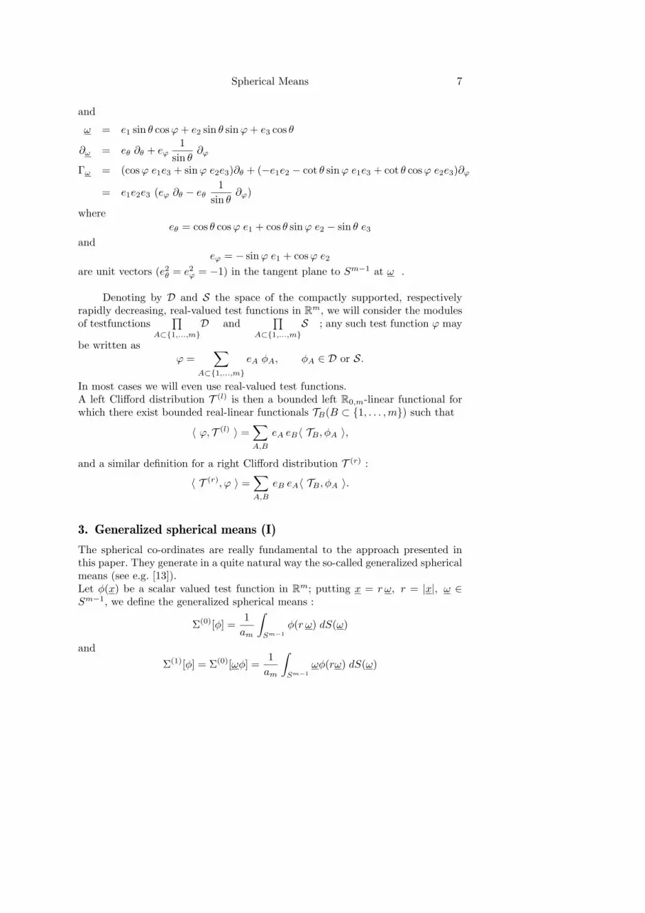
and

ω = e1 sin θ cosϕ+ e2 sin θ sinϕ+ e3 cos θ

∂ω = eθ ∂θ + eϕ1

sin θ∂ϕ

Γω = (cosϕ e1e3 + sinϕ e2e3)∂θ + (−e1e2 − cot θ sinϕ e1e3 + cot θ cosϕ e2e3)∂ϕ

= e1e2e3 (eϕ ∂θ − eθ1

sin θ∂ϕ)

whereeθ = cos θ cosϕ e1 + cos θ sinϕ e2 − sin θ e3

andeϕ = − sinϕ e1 + cosϕ e2

are unit vectors (e2θ = e2ϕ = −1) in the tangent plane to Sm−1 at ω .

Denoting by D and S the space of the compactly supported, respectivelyrapidly decreasing, real-valued test functions in R

m, we will consider the modulesof testfunctions

∏A⊂1,...,m

D and∏

A⊂1,...,m

S ; any such test function ϕ may

be written asϕ =

∑

A⊂1,...,m

eA φA, φA ∈ D or S.

In most cases we will even use real-valued test functions.A left Clifford distribution T (l) is then a bounded left R0,m-linear functional forwhich there exist bounded real-linear functionals TB(B ⊂ 1, . . . ,m) such that

〈 ϕ, T (l) 〉 =∑

A,B

eA eB〈 TB , φA 〉,

and a similar definition for a right Clifford distribution T (r) :

〈 T (r), ϕ 〉 =∑

A,B

eB eA〈 TB , φA 〉.

3. Generalized spherical means (I)

The spherical co-ordinates are really fundamental to the approach presented inthis paper. They generate in a quite natural way the so-called generalized sphericalmeans (see e.g. [13]).Let φ(x) be a scalar valued test function in R

m; putting x = r ω, r = |x|, ω ∈Sm−1, we define the generalized spherical means :

Σ(0)[φ] =1

am

∫

Sm−1

φ(r ω) dS(ω)

and

Σ(1)[φ] = Σ(0)[ωφ] =1

am

∫

Sm−1

ωφ(rω) dS(ω)


where dS(ω) denotes the Lebesgue measure on Sm−1.

Note that Σ(0)[φ] is nothing else but the classical spherical mean introduced byJohn in [10].

The generalized spherical means enjoy the following properties. Firstly wenote that both spherical means are interrelated by the action of the Dirac operator.In accordance with [13] we have, extending the notion of spherical mean to Cliffordalgebra valued, in casu vector valued, functions :

Proposition 3.1. For a scalar valued test function φ one has

(i)

Σ(0)[∂φ] =

(∂r +

m− 1

r

)Σ(1)[φ]

(ii)

Σ(1)[∂φ] = − ∂r Σ(0)[φ]

(iii)

Σ(0)[∂ωφ] = (m− 1) Σ(1)[φ]

(iv)

Σ(1)[∂ωφ] = 0

Proof

Consider the ball B(0, ρ) with arbitrary radius ρ > 0 and apply Stokes’s Theorem(see [2]) to obtain:

∫

B(0,ρ)

∂φ dV (x) =

∫

∂B(0,ρ)

dσ φ = ρm−1

∫

Sm−1

ω φ(ρω) dS(ω)

For the left hand side we get:∫ ρ

0

rm−1 dr

∫

Sm−1

(ω ∂rφ+

1

r∂ωφ

)dS(ω)

=

∫

Sm−1

dS(ω) ω

∫ ρ

0

rm−1 ∂rφ dr +

∫ ρ

0

rm−2 dr

∫

Sm−1

∂ωφ dS(ω)

= ρm−1

∫

Sm−1

ω φ(ρω) dS(ω) +

∫ ρ

0

rm−2 dr

∫

Sm−1

(∂ωφ− (m− 1) ω φ

)dS(ω)

As the first term in the last expression equals the right hand side of the aboveStokes Formula, it follows that

∫

Sm−1

∂ωφ dS(ω) = (m− 1)

∫

Sm−1

ω φ dS(ω)

or Σ(0)[∂ωφ] = (m− 1) Σ(1)[φ], which proves formula (iii).

Spherical Means 9

Next we have:

am Σ(0)[∂φ] =

∫

Sm−1

∂φ dS(ω) =

∫

Sm−1

(ω ∂rφ+

1

r∂ωφ

)dS(ω)

= am ∂r Σ(1)[φ] + am1

rΣ(0)[∂ωφ] = am

(∂r +

m− 1

r

)Σ(1)[φ]

which proves formula (i).

Now apply again Stokes’s Theorem to obtain∫

B(0,ρ)

(x φ) ∂ dV (x) =

∫

∂B(0,ρ)

x φ dσ = − ρm∫

Sm−1

φ(ρω) dS(ω)

For the left hand side we get:∫

B(0,ρ)

(x ∂φ−m φ) dV (x) =

= −m

∫ ρ

0

rm−1 Σ(0)[φ] dr −

∫ ρ

0

rm dr

∫

Sm−1

∂rφ dS(ω) +

∫ ρ

0

rm−1 Σ(1)[∂ωφ] dr

= − ρm∫

Sm−1

φ(ρω) dS(ω) +

∫ ρ

0

rm−1 Σ(1)[∂ωφ] dr

As the first term in the last expression equals the right hand side of the aboveStokes Formula, formula (iv) follows.Finally,

am Σ(1)[∂φ] =

∫

Sm−1

ω

(ω ∂rφ+

1

r∂ωφ

)dS(ω)

= − Σ(0)[∂rφ] +1

rΣ(1)[∂ωφ] = − ∂r Σ(0)[φ]

proving formula (ii).

Proposition 3.2. If φ(x) is a scalar valued test function, then the spherical mean

Σ(0)[φ] is an even, scalar valued test function on the real r-axis; its derivatives of

odd order vanish at the origin r = 0, while for its derivatives of even order one

has ∂2lφ(x)

x=0= (−1)lC(l)

∂2lr Σ(0)[φ]

r=0

or, equivalently, in terms of distributions:

〈 ∂2lδ(x), φ(x) 〉 = (−1)l C(l)〈 ∂2lr δ(r),Σ(0)[φ] 〉.

where

C(l) =22ll!

(2l)!

(m2

+ l − 1). . .

(m2

)=

22ll!

(2l)!

Γ(m2 + l)

Γ(m2 ), l = 0, 1, 2, . . .


Proof

We prove the formula for the derivatives of even order by induction on l.For l = 0 we have to prove that

〈 δ(x) , φ(x) 〉 = 〈 δ(r) , Σ(0)[φ] 〉

or

φ(0) =

1

am

∫

Sm−1

φ(rω) dS(ω)

r=0

which is of course valid.For l = 1 we have to prove that

〈 −∆δ(x) , φ(x) 〉 = −m 〈 δ′′(r) , Σ(0)[φ] 〉

Indeed, we have

am Σ(0)[∆φ] =

∫

Sm−1

∆φ dS(ω)

=

∫

Sm−1

(∂2r +

m− 1

r∂r +

1

r2∆∗

)φ(rω) dS(ω)

= am

(∂2r +

m− 1

r∂r

)Σ(0)[φ]

since ∫

Sm−1

∆∗φ(rω) dS(ω) = 0

It thus follows thatΣ(0)[∆φ]

r=0= lim

r→>0

(∂2r +

m− 1

r∂r

)Σ(0)[φ] = m

∂2r Σ(0)[φ]

r=0

and hence, in view of the result for l = 0,

〈 ∆δ(x) , φ(x) 〉 = 〈 δ(x) , ∆φ 〉

= 〈 δ(r) , Σ(0)[∆φ] 〉 = m 〈 δ′′(r) , Σ(0)[φ] 〉

which proves the formula for l = 1.Now assume the formula to be valid for l; then we have consecutively:

〈 ∂2l+2δ(x) , φ(x) 〉 = 〈 ∂2lδ(x) , ∆φ 〉

= (−1)l C(l) 〈 ∂2lr δ(r) , Σ(0)[∆φ] 〉

= (−1)l C(l) 〈 ∂2lr δ(r) ,

(∂2r +

m− 1

r∂r

)Σ(0)[φ] 〉

= (−1)l C(l) 〈 ∂2l+2r δ(r) , Σ(0)[φ] 〉+ (−1)l C(l)

m− 1

2l + 1〈 ∂2l+2

r δ(r) , Σ(0)[φ] 〉

= (−1)l+1 C(l + 1) 〈 ∂2l+2r δ(r) , Σ(0)[φ] 〉

Spherical Means 11

which proves the formula for l + 1.

Proposition 3.3. If φ(x) is a scalar valued test function, then the spherical mean

Σ(1)[φ] is an odd, vector valued test function on the real r-axis; its derivatives of

even order vanish at the origin r = 0, while for the derivatives of odd order one

has ∂2l+1φ(x)

x=0= (−1)lC(l + 1)

∂2l+1r Σ(1)[φ]

r=0

or, equivalently, in terms of distributions:

〈 ∂2l+1δ(x), φ(x) 〉 = (−1)l C(l + 1)〈 ∂2l+1r δ(r),Σ(1)[φ] 〉

Proof

We prove the formula for the derivatives of odd order. Let φ be a scalar valuedtest function. Then by Proposition 3.2 and Proposition 3.1, we have:

〈 ∂2l+1δ(x) , φ(x) 〉 = −〈 ∂2lδ(x) , ∂φ 〉

= (−1)l+1 C(l) 〈 ∂2lr δ(r) , Σ(0)[∂φ] 〉

= (−1)l+1 C(l) 〈 ∂2lr δ(r) ,

(∂r +

m− 1

r

)Σ(1)[φ] 〉

= (−1)l C(l) 〈 ∂2lr δ(r) , Σ(1)[φ] 〉+

m− 1

2l + 1(−1)l C(l) 〈 ∂2l+1

r δ(r) , Σ(1)[φ] 〉

= (−1)l+1 C(l + 1) 〈 ∂2l+1r δ(r) , Σ(1)[φ] 〉

Note that in particular Σ(0)[φ]r=0 = φ(0), while Σ(1)[φ]r=0 = 0 or∫

Sm−1

ω dS(ω) = 0

4. Classical and Clifford distributions in Euclidean space

In this section we will define classical and new distributions in the Clifford settingmaking use of the spherical co-ordinates, the fundamental distribution Fp r

µ+ of

section 1 and the spherical means of section 3.

Let us explain the underlying idea by considering the special case of a locallyintegrable radial function T (r). Its action as a regular distribution on a scalarvalued test function φ(x) is given by

〈 T (r), φ(x) 〉 =

∫

Rm

T (r) φ(x) dV (x),


dV (x) denoting the Lebesgue measure in Rm.

Introducing spherical co-ordinates this integral takes the form∫ +∞

0

T (r)rm−1dr

∫

Sm−1

φ(rω)dS(ω) =

∫ +∞

0

T (r)rm−1Σ(0)[φ] dr.

Hence for T (r) = rλ with Reλ > −m, we find

〈 rλ, φ(x) 〉 =

∫ +∞

0

rµΣ(0)[φ] dr = 〈 rµ+,Σ(0)[φ] 〉

where we have put µ = λ +m − 1. By this procedure the action of the distribu-tion T (r) = rλ in R

m is converted into an action of the distribution rµ+ on the realline. It is this conversion which is used in defining our Clifford distributions in R

m.

Let λ be a complex parameter and let φ be a scalar valued test function. Wedefine the scalar valued distributions Tλ and the vector valued distributions Uλ

by:

〈 Tλ, φ 〉 = am〈 Fp rµ+, Σ(0)[φ] 〉

and

〈 Uλ, φ 〉 = am〈 Fp rµ+, Σ(1)[φ] 〉

where we have put

µ = λ+m− 1.

These distributions are classical, in the sense as explained in the introduction:the Tλ distributions appear in harmonic analysis where they are sometimes denotedby Fp rλ, while the Uλ distributions – at least some of them – appear in Cliffordanalysis. More familiar expressions are given in the next proposition.

Proposition 4.1. For µ = λ+m− 1 such that −2l − 1 < Reµ < −2l + 1 one has

〈 Tλ, φ 〉 = limε→

>0

∫

Rm\B(0,ε)

rλφ(x) dV (x) +

l∑

j=0

C(j)(∆jφ)(0)ελ+m+2j

λ+m+ 2j

while for l = 0, 1, 2, . . .

〈 T−m−2l, φ 〉 =

limε→

>0

∫

Rm\B(0,ε)

r−m−2lφ(x) dV (x) +

l−1∑

j=0

C(j)(∆jφ)(0)ε2j−2l

2j − 2l+ C(l)(∆lφ)(0) ln ε

with

C(j) = am1

(2j)!

1

C(j)= am

1

22jj!(m2 + j − 1) . . . (m2 )

= πm/2 1

22j−1j!Γ(m2 + j), j = 0, 1, 2, . . .

Spherical Means 13

Note that the first formula is in accordance with [11].Examples of the Tλ and Uλ distributions are given in the next section.

5. The action of the Dirac operator on the distributions Tλ and Uλ

As the distributions Tλ are scalar valued it is not necessary to distinguish betweenan action of the Dirac operator from the left or from the right. The results of thataction, ∂Tλ, will be vector valued distributions, and as long as the testfunctions φremain scalar valued it is neither necessary to distinguish between ∂Tλ as to be aleft or a right distribution.

Proposition 5.1. For λ ∈ C\−m− 2l : l = 0, 1, 2, . . . one has

∂Tλ = λ Uλ−1

and in particular ∂T0 = ∂1x = 0, while for l = 0, 1, 2, . . .

∂ T−m−2l = −(m+ 2l)U−m−2l−1 + (−1)l+12(l + 1) C(l + 1) ∂2l+1δ(x)

and

∂ ln r = U−1

Proof

Firstly we proof the formula in the general case where λ 6= −m−n, n = 0, 1, 2, . . ..For any scalar valued test function φ we have by the definition of the derivative ofa distribution:

〈 ∂ Tλ , φ 〉 = − 〈 Tλ , ∂ φ 〉

By the definition of the distributions Tλ, this equals

− am 〈 Fp rµ+ , Σ(0)[∂ φ] 〉

which, by Proposition 3.1, is turned into

− am〈 Fp rµ+ ,

(∂r +

m− 1

r

)Σ(1)[φ] 〉

= am〈 ∂r Fp rµ+ , Σ(1)[φ] 〉 − am (m− 1)〈 Fp rµ−1

+ , Σ(1)[φ] 〉

= am (µ−m+ 1) 〈 Fp rµ−1+ , Σ(1)[φ] 〉

= λ 〈 Uλ−1 , φ 〉

Now for the exceptional cases where λ = −m− 2l, l = 0, 1, 2, . . ., we have consec-utively, taking Lemma 1.1 into account:

〈 ∂ T−m−2l, φ 〉 = − 〈 T−m−2l, ∂ φ 〉


= − am 〈 Fp r−2l−1+ , Σ(0)[∂ φ] 〉

= − am 〈 Fp r−2l−1+ ,

(∂r +

m− 1

r

)Σ(1)[φ] 〉

= am 〈 ∂r Fp r−2l−1+ , Σ(1)[φ] 〉 − am(m− 1)〈 Fp r−2l−2

+ , Σ(1)[φ] 〉

= −(m+ 2l) am〈 Fp r−2l−2+ , Σ(1)[φ] 〉

+am(−1)2l+1 1

(2l + 1)!〈 δ

(2l+1)(r) , Σ(1)[φ] 〉

= −(m+ 2l)am〈 Fp r−2l−2+ , Σ(1)[φ] 〉

+am(−1)2l+1 1

(2l + 1)!

(−1)l

C(l + 1)〈 ∂2l+1δ(x) , φ(x) 〉

whence

∂T−m−2l = −(m+ 2l)U−m−2l−1 + am(−1)l+1 ∂2l+1δ(x)

22l+1l!(m2 + l

). . .

(m2

)

The exceptional cases where λ = −m − 2l − 1, l = 0, 1, 2, . . . are treated ina similar manner; there is however no singular term involving derivatives of thedelta distribution, since the even order derivatives of Σ(1)[φ] vanish at r = 0.Finally we also have

〈 ∂ ln r , φ 〉 > = − 〈 ln r , ∂φ 〉

=

∫ +∞

0

rm−1 ln r dr

∫

Sm−1

∂φ dS(ω)

= −

∫ +∞

0

rm−1 ln r ∂rΣ(1)[φ] dr − (m− 1)

∫ +∞

0

rm−2 ln r Σ(1)[φ] dr

=

∫ +∞

0

rm−2 Σ(1)[φ] dr

= 〈 Fp rm−2+ , Σ(1)[φ] 〉 = 〈 U−1 , φ 〉

As the distributions Uλ are vector valued, we should, a priori, make a dis-tinction between an action from the left or an action from the right of the Diracoperator and at the same time consider ∂Uλ as a left distribution, respectivelyUλ∂ as a right distribution. Both cases can be treated similarly and it turns outthat both actions lead to the same scalar valued distribution.

Proposition 5.2. For λ ∈ C\−m− 2l − 1 : l = −1, 0, 1, 2, . . . one has

∂Uλ = Uλ∂ = −(λ+m− 1)Tλ−1

Spherical Means 15

while for l = 0, 1, 2, . . .

∂U−m−2l−1 = U−m−2l−1 ∂ = (2l + 2)T−m−2l−2 − C(l + 1)∆l+1δ(x)

and

∂U−m+1 = U−m+1 ∂ = −amδ(x)

Proof

Firstly we proof the formula in the general case where λ 6= −m − n, n =−1, 0, 1, 2, . . .For any scalar valued test function φ one has, considering right distributions,

〈 Uλ∂ , φ 〉 = −〈 Uλ , ∂φ 〉

= −am 〈 Fp rµ+ , Σ(1)[∂φ] 〉 = −am 〈 Fp rµ+ , −∂rΣ(0)[φ] 〉

= −am 〈 µ Fp rµ−1+ , Σ(0)[φ] 〉 = −(λ+m− 1) 〈 Tλ−1 , φ 〉

Next for the exceptional case where λ = −m+ 1 we get:

〈 U−m+1∂ , φ 〉 = −〈 U−m+1 , ∂φ 〉

= −am 〈 Fp r0+ , Σ(1)[∂φ] 〉 = −am 〈 Y (r) , −∂rΣ(0)[φ] 〉

= −am 〈 δ(r) , Σ(0)[φ] 〉 = −am 〈 δ(x) , φ(x) 〉

Finally for the exceptional cases where λ = −m − 2l − 1, l = 0, 1, 2, . . . we have,taking Lemma 1.1 into account:

〈 U−m−2l−1 ∂, φ 〉 = −〈 U−m−2l−1, ∂φ 〉 = −am〈 Fp r−2l−2+ ,Σ(1)[∂ φ] 〉

= −am〈 Fp r−2l−2+ ,−∂rΣ

(0)[φ] 〉 = −am〈 ∂rFp r−2l−2+ ,Σ(0)[φ] 〉

= −am〈 (−2l − 2)Fp r−2l−3+ +

1

(2l + 2)!δ(2l+2)(r) ,Σ(0)[φ] 〉

= am(2l + 2)〈 Fp r−2l−3+ ,Σ(0)[φ] 〉 − am

1

(2l + 2)!〈 δ

(2l+2)(r) ,Σ(0)[φ] 〉

whence

U−m−2l−1 ∂ = (2l + 2)T−m−2l−2 − (−1)l+1 am

(2l + 2)!C(l + 1)∂2l+2δ(x)

or still

U−m−2l−1 ∂ = (2l + 2)T−m−2l−2 − C(l + 1)∆l+1δ(x).

The exceptional cases where λ = −m − 2l, l = 0, 1, 2, . . . are treated in a simi-lar manner; there is however no singular term involving derivatives of the deltadistribution, since the odd order derivatives of Σ(0)[φ] vanish at r = 0.


Remark 5.3. The proofs of Propositions 5.1 and 5.2 are fundamental; they nicelydemonstrate the technique as explained at the beginning of this section. The proofsof the similar propositions in the rest of the paper run along the same lines andwill not be given anymore.

6. Some specific distributions in Euclidean space

In this section we give some explicit examples of the distributions Tλ and Uλ

introduced in the foregoing sections. It is shown that for specific values of theparameter λ, distributions are obtained which were already known in Cliffordanalysis, thus illustrating the unifying character of our approach.

6.1.

For λ = 0 we have

〈 U0, φ 〉 = am〈 Fp rm−1+ ,Σ(1)[φ] 〉 =

∫ +∞

0

rm−1 dr

∫

Sm−1

ωφ(rω) dS(ω)

=

∫

Rm

ω φ(x) dV (x)

in other words U0(x) is the locally integrable function ω.We also have

∂ T1 = ∂r = U0 = ω,

and

∂ ω = ω ∂ = −(m− 1)T−1 = −(m− 1)1

r= −∆r

and also

∆ω = (m− 1)∂1

r= −(m− 1)U2 = (m− 1)

ω

r2.

The distribution ω is the higher dimensional analogue of the one dimensional”signum”-distribution

sgn(x) =

−1 , x < 01 , x > 0

6.2.

For λ = −m we have

〈 U−m, φ 〉 = am〈 Fp r−1+ ,Σ(1)[φ] 〉 =

∫ +∞

0

1

rdr

∫

Sm−1

ωφdS(ω)

=

∫

Rm

ω

rm(φ(x)− φ(0))dV (x) = lim

ε→>0

∫

Rm\B(0,ε)

ω

rmφ(x)dV (x)

so that (see e.g. [5])

U−m = −Pvω

rm

Spherical Means 17

where Pv stands for ”principal value”. It is the higher dimensional analogue of theone dimensional Pv 1

x distribution given by

〈 Pv1

x, φ(x) 〉 = lim

ε→>0

(∫ −ε

−∞

+

∫ +∞

ε

φ(x)

xdx

)=

∫ +∞

−∞

φ(x)− φ(o)

xdx.

For this distribution U−m we have the following formulae:

(i) rmω Pvω

rm= 1

(ii) Pvω

rm=

1

m− 1∂

1

rm−1

(iii) ∂

(Pv

ω

rm

)= −∂ U−m = −T−m−1 = −Fp

1

rm+1

(iv) ∆

(Pv

ω

rm

)= ∂(T−m−1) = −(m+ 1)U−m−2 = (m+ 1)Fp

ω

rm+2

As ∫

Sm−1

ω dS(ω) = 0

(see section 3) the distribution Pv ωrm is a typical example of a convolution oper-

ator (see [9], [12]):

Pvω

rm∗ φ = lim

ε→>0

∫

Rm\B(0,ε)

y − x

|y − x|

φ(x)

|y − x|mdV (x)

giving rise to the Hilbert transform of the test function φ (see [8] and [5]).

6.3.

Start with the observation that, according to Proposition I.5.2, we have for λ =−m+ 1:

∂ U−m+1 = U−m+1 ∂ = −am δ(x)

confirming that

−1

amU−m+1 =

1

am

ω

rm−1

is the fundamental solution of the Dirac operator in Rm (see section 2).

Next, observe that, according to the Proposition 5.1, we have:

∂2T−m+2 = ∂((−m+ 2)U−m+1)) = (m− 2)am δ(x)

confirming that

−1

am

1

m− 2T−m+2 = −

1

am

1

m− 2

1

rm−2

is the fundamental solution of the Laplace operator in Rm.

Hence, find recursively the fundamental solutions of the natural powers of theDirac operator, and at the same time of the Laplace operator, to be:

∂2l(

1

2l − 2. . .

1

4

1

2

1

am

1

m− 2

1

m− 4. . .

1

m− 2lT−m+2l

)= δ(x)


and

∂2l+1

(−

1

2l. . .

1

4

1

2

1

am

1

m− 2

1

m− 4. . .

1

m− 2lU−m+2l+1

)= δ(x)

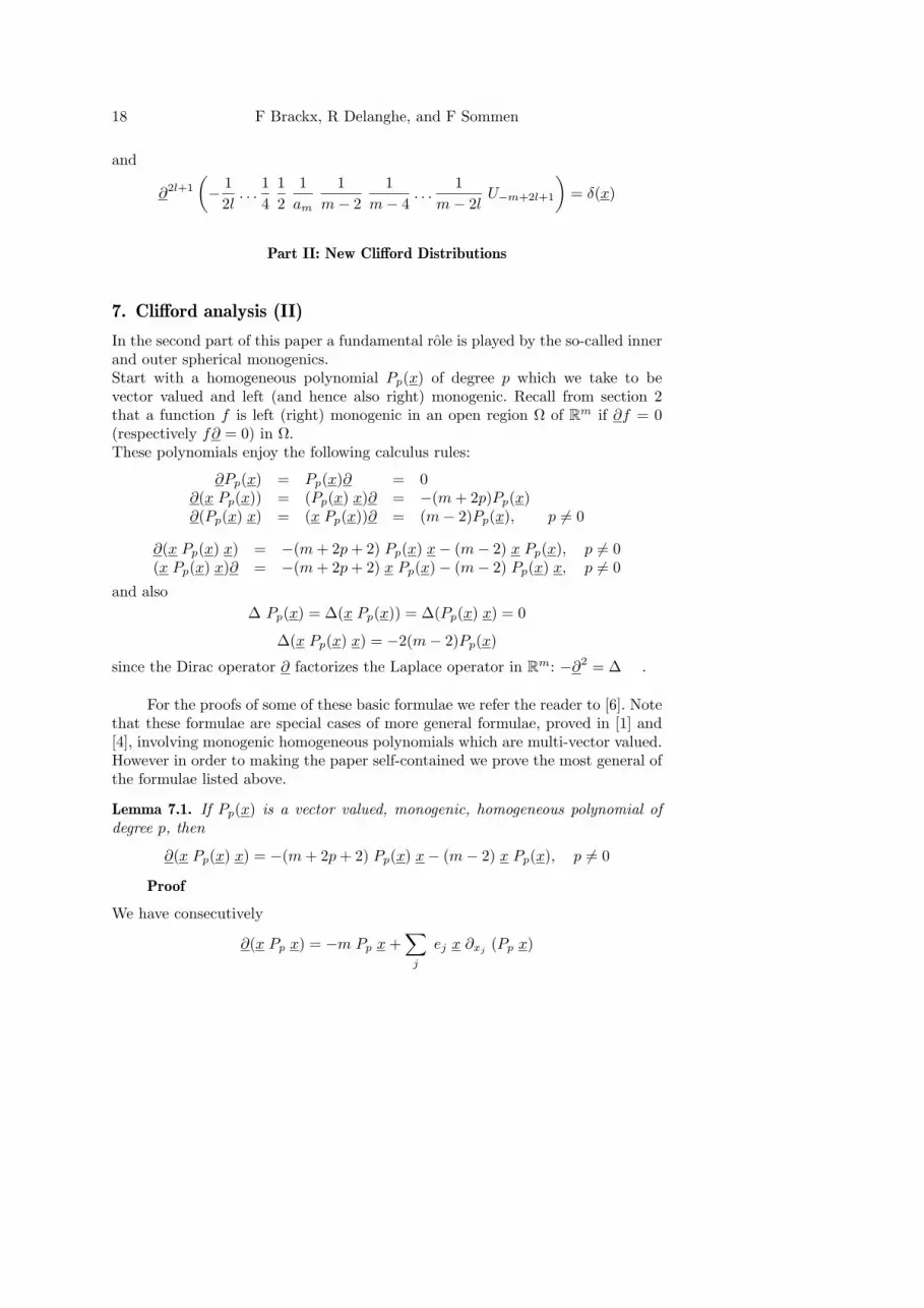
Part II: New Clifford Distributions

7. Clifford analysis (II)

In the second part of this paper a fundamental role is played by the so-called innerand outer spherical monogenics.Start with a homogeneous polynomial Pp(x) of degree p which we take to bevector valued and left (and hence also right) monogenic. Recall from section 2that a function f is left (right) monogenic in an open region Ω of Rm if ∂f = 0(respectively f∂ = 0) in Ω.These polynomials enjoy the following calculus rules:

∂Pp(x) = Pp(x)∂ = 0∂(x Pp(x)) = (Pp(x) x)∂ = −(m+ 2p)Pp(x)∂(Pp(x) x) = (x Pp(x))∂ = (m− 2)Pp(x), p 6= 0

∂(x Pp(x) x) = −(m+ 2p+ 2) Pp(x) x− (m− 2) x Pp(x), p 6= 0(x Pp(x) x)∂ = −(m+ 2p+ 2) x Pp(x)− (m− 2) Pp(x) x, p 6= 0

and also

∆ Pp(x) = ∆(x Pp(x)) = ∆(Pp(x) x) = 0

∆(x Pp(x) x) = −2(m− 2)Pp(x)

since the Dirac operator ∂ factorizes the Laplace operator in Rm: −∂2 = ∆ .

For the proofs of some of these basic formulae we refer the reader to [6]. Notethat these formulae are special cases of more general formulae, proved in [1] and[4], involving monogenic homogeneous polynomials which are multi-vector valued.However in order to making the paper self-contained we prove the most general ofthe formulae listed above.

Lemma 7.1. If Pp(x) is a vector valued, monogenic, homogeneous polynomial of

degree p, then

∂(x Pp(x) x) = −(m+ 2p+ 2) Pp(x) x− (m− 2) x Pp(x), p 6= 0

Proof

We have consecutively

∂(x Pp x) = −m Pp x+∑

j

ej x ∂xj(Pp x)

Spherical Means 19

= −m Pp x−∑

j

x ej ∂xj (Pp x)− 2∑

j

xj ∂xj (Pp x)

= (−m− 2p− 2) Pp x− x ∂(Pp x)

= −(m+ 2p+ 2) Pp x− (m− 2) x Pp

since

∂(Pp x) =∑

j

ej Pp ej = m Pp − 2 Pp

These vector valued monogenic homogeneous polynomials Pp(x) may be re-alized under the action of the Dirac operator upon real-valued harmonic homoge-neous polynomials Sp+1 of degree (p+ 1):

Pp(x) = ∂ Sp+1(x)

We then have

x Pp(x) = x • ∂ Sp+1(x) + x ∧ ∂ Sp+1(x)

and

Pp(x) x = x • ∂ Sp+1(x)− x ∧ ∂ Sp+1(x)

from which it follows that

x Pp(x) + Pp(x) x = 2x • ∂ Sp+1(x) = −2〈 x, ∂ 〉 Sp+1(x) = −2(p+ 1)Sp+1(x)

is scalar valued.

By taking restrictions of the polynomials Pp(x) to the unit sphere Sm−1 , weobtain so-called inner spherical monogenics Pp(ω), for which the following formulae


hold:

∂ Pp(ω) = −p

rω Pp(ω)

Pp(ω)∂ = −p

rPp(ω) ω

∂ω Pp(ω) = −p ω Pp (ω)

Pp(ω) ∂ω = −p Pp(ω) ω

ω ∂ω Pp(ω) = Pp(ω)∂ω ω = p Pp(ω)

∂ω(ω Pp(ω)) = (Pp(ω)ω)∂ω = −(m+ p− 1)Pp(ω)

∂ω(Pp(ω) ω) = (ω Pp(ω))∂ω = (m− 2)Pp(ω)− (p+ 1)ω Pp(ω) ω, p 6= 0

∂ω(ω Pp(ω) ω) = −(m+ p)Pp(ω) ω − (m− 2)ω Pp(ω), p 6= 0

(ω Pp(ω) ω)∂ω = −(m+ p) ω Pp(ω)− (m− 2)Pp(ω) ω, p 6= 0

∂2ω Pp(ω) = Pp(ω) ∂2ω = p(m+ p− 1) Pp(ω)

∆∗ Pp(ω) = (−p)(p+m− 2) Pp(ω)

Note again that these formulae are special cases of more general ones, proved in [1],involving multi-vector spherical monogenics; however as an illustration we provethe following

Lemma 7.2. If Pp(ω) is a vector valued spherical monogenic of degree p then

∂ω(Pp(ω) ω) = −(p+ 1) ω Pp(ω) + (m− 2) Pp(ω)

Proof

Using the expression of the Dirac operator in spherical co-ordinates, we have con-secutively

∂ω(Pp(ω) ω) = r ∂(Pp(ω) ω) = r ∂(1

rp+1Pp(x) x)

= r (∂1

rp+1) Pp(x) x+

1

rp∂(Pp(x) x)

= ω (−p− 1)1

rp+1Pp(x) x+

1

rp(m− 2) Pp(x)

= −(p+ 1) ω Pp(ω) ω + (m− 2) Pp(ω)

Given an inner spherical monogenic Pp(ω) then obviously

rp Pp(ω) = Pp(x)

Spherical Means 21

is a left and right monogenic homogeneous polynomial the restriction of which tothe unit sphere is precisely Pp(ω).At the same time the functions

1

rm+p−1ω Pp(ω) =

1

rm+2px Pp(x) = Q(l)

p (x)

and1

rm+p−1Pp(ω) ω =

1

rm+2pPp(x) x = Q(r)

p (x)

are left, respectively right, monogenic homogeneous functions of order −(m+p−1)in the complement of the origin. Their restrictions to the unit sphere Sm−1:

Q(l)p = ω Pp(ω) and Q(r)

p = Pp(ω) ω

are called outer spherical monogenics.With the above notations we have:

ω Pp(ω) + Pp(ω) ω = −2(p+ 1) Sp+1(ω)

Also note that the inner spherical monogenics Pp(ω) and the outer spherical mono-genics ω Pp(ω) and Pp(ω) ω are special cases of spherical harmonics.

8. Generalized spherical means (II)

In section 3 we studied the generalized spherical means Σ(0) and Σ(1) used after-wards in the definition of the distributions Tλ and Uλ. In view of the definition ofnew distributions in section 9 in which the spherical monogenics will play a role,we now introduce the necessary corresponding spherical means.

Let φ(x) be a scalar valued test function in Rm, and let Pp(x) be a vector

valued, monogenic, homogeneous polynomial of degree p 6= 0 as introduced in theprevious section 7. The spherical mean Σ(0) of part I is now generalized, dependingon the parity of p, as follows:

Σ(0)2k [φ] = Σ(0)[P2k(ω)φ(x)] =

1

am

∫

Sm−1

P2k(ω)φ(x) dS(ω), k = 1, 2, . . .

and

Σ(0)2k+1[φ] = Σ(0)[r P2k+1(ω)φ(x)] =

r

am

∫

Sm−1

P2k+1(ω)φ(x) dS(ω), k = 0, 1, 2, . . .

Note that if p = 0 and P0(x) = 1, then Σ(0)0 [φ] = Σ(0)[φ].

Note also the extra factor r in the definition of Σ(0)2k+1; in this way this spherical

mean vanishes at the origin r = 0 (a property which will exploited in the sequel)

and moreover the formulae established for Σ(0)2k+1 and Σ

(0)2k become symmetric.

We now examine the behaviour at the origin r = 0 of the derivatives of thesevector valued spherical means .


Proposition 8.1. If φ(x) is a scalar valued test function, then the spherical means

Σ(0)p [φ] are even test functions on the real r-axis, with derivatives of odd order

vanishing at the origin r = 0, while for the derivatives of even order one has:

∂2lr Σ

(0)2k [φ]

r=0=

(2l)!

(2k + 2l)!

1

C(k + l)

∆k+l

m (φ(x)P2k(x))x=0

and∂2lr Σ

(0)2k+1[φ]

r=0=

(2l)!

(2k + 2l)!

1

C(k + l)

∆k+l

m (φ(x)P2k+1(x))x=0

Proof

First consider the case where p = 2k and observe that

Σ(0)[P2k(x)φ(x)] = r2k Σ(0)[P2k(ω)φ(x)] = r2k Σ(0)2k [φ]

whence ∂2k+jr Σ(0)[P2k(x)φ(x)]

r=0=

(2k + j)!

j!

∂jrΣ

(0)2k [φ]

r=0

If j = 2l + 1, then ∂2l+1r Σ

(0)2k [φ]

r=0= 0

while for j = 2l we get∂2lr Σ

(0)2k [φ]

r=0=

(2l)!

(2k + 2l)!

∂2k+2lr Σ(0)[P2k(x)φ(x)]

r=0

= (−1)k+l (2l)!

(2k + 2l)!

1

C(k + l)

∂2k+2l(φ(x)P2k(x))

x=0

In the case where p = 2k + 1, start with

Σ(0)[P2k+1(x)φ(x)] = r2kΣ(0)[r P2k+1(ω)φ(x)] = r2k Σ(0)2k+1[φ]

to obtain, in a similar way, the desired result.

Remark 8.2. The above results for the values at the origin of the even order

derivatives of the spherical means Σ(0)p [φ] may be rewritten in terms of distributions

as: ∂2lr Σ

(0)2k [φ]

r=0=

(2l)!

(2k + 2l)!

1

C(k + l)〈 P2k(x) ∆

k+lm δ(x), φ(x) 〉

and∂2lr Σ

(0)2k+1[φ]

r=0=

(2l)!

(2k + 2l)!

1

C(k + l)〈 P2k+1(x) ∆

k+lm δ(x), φ(x) 〉

where the obtained vector valued distributions may act from the left as well asfrom the right.

Spherical Means 23

Remark 8.3. As Pp(ω) is a spherical harmonic, we have that∫

Sm−1

Pp(ω) dS(ω) = 0, p = 1, 2, 3, . . .

while for p = 0 : ∫

Sm−1

dS(ω) = am

HenceΣ

(0)2k [φ]

r=0=

1

(2k)!

1

C(k)

∆k(φ(x)P2k(x))

x=0

= 0 , k 6= 0

while Σ

(0)0 [φ]

r=0= φ(0)

The spherical mean Σ(1)[φ] of part I is now generalized as follows:

(i) Σ(1)2k [φ] = Σ(0)[ω P2k(ω)φ(x)] =

1

am

∫

Sm−1

ω P2k(ω)φ(x) dS(ω)

(ii) Σ(1)2k+1[φ] = Σ(0)[r ω P2k+1(ω)φ(x)] =

r

am

∫

Sm−1

ω P2k+1(ω)φ(x) dS(ω)

(iii) Σ(3)2k [φ] = Σ(0)[P2k(ω) ω φ(x)] =

1

am

∫

Sm−1

P2k(ω) ω φ(x) dS(ω)

(iv) Σ(3)2k+1[φ] = Σ(0)[P2k+1(ω) r ω φ(x)] =

r

am

∫

Sm−1

P2k+1(ω) ω φ(x) dS(ω).

Note that if p = 0 and P0(x) = 1 then Σ(1)0 [φ] = Σ

(3)0 [φ] = Σ(1)[φ].

The next proposition summarizes the properties of these spherical means; its proofis similar to that of Proposition 8.1.

Proposition 8.4. If φ(x) is a scalar valued test function, then the spherical means

Σ(1)p [φ] and Σ

(3)p [φ] are odd test functions on the real r-axis with derivatives of even

order vanishing at r = 0, while for the derivatives of odd order one has:∂2l+1r Σ

(1)2k [φ]

r=0=

(−1)k+l+1 (2l + 1)!

(2k + 2l + 1)!

1

C(k + l + 1)〈(∂2k+2l+1δ(x)

)P2k(x), φ(x) 〉

∂2l+1r Σ

(1)2k+1[φ]

r=0=

(−1)k+l+1 (2l + 1)!

(2k + 2l + 1)!

1

C(k + l + 1)〈(∂2k+2l+1δ(x)

)P2k+1(x), φ(x) 〉


∂2l+1r Σ

(3)2k [φ]

r=0=

(−1)k+l+1 (2l + 1)!

(2k + 2l + 1)!

1

C(k + l + 1)〈 P2k(x)

(∂2k+2l+1δ(x)

), φ(x) 〉

∂2l+1r Σ

(3)2k+1[φ]

r=0=

(−1)k+l+1 (2l + 1)!

(2k + 2l + 1)!

1

C(k + l + 1)〈 P2k+1(x)

(∂2k+2l+1δ(x)

), φ(x) 〉

Remark 8.5. The above obtained distributional expressions need an additionalconsideration w.r.t. left or right action upon the test function φ. We focus on onecase :

∂2k+2l+1(P2k(x)φ(x))

x=0

the other cases being treated similarly.If left action on the test function is concerned, we have readily

〈 δ(x), ∂2k+2l+1(P2k(x)φ(x) 〉 = −〈 ∂2k+2l+1δ(x), P2k(x)φ(x) 〉

= −〈 (∂2k+2l+1δ(x))P2k(x), φ(x) 〉.

In the case of right action on the test function, we have

〈 ∂2k+2l+1(P2k(x)φ(x)), δ(x) 〉

= 〈 (−1)k+l∂ ∆k+lm (P2k(x)φ(x)), δ(x) 〉

= (−1)k+l〈 ∂(P2k(x)φ(x)),∆k+lm δ(x) 〉

= (−1)k+l〈 ∂ φ(x)P2k(x),∆k+lm δ(x) 〉

= (−1)k+l〈 ∂ φ(x), P2k(x)(∆k+lm δ(x)) 〉

= (−1)k+l+1〈 φ(x), ∂(P2k(x)(∆k+lm δ(x))) 〉

= (−1)k+l+1〈 φ(x), ∂(∆k+lm δ(x))P2k(x) 〉

= − 〈 φ(x), (∂2k+2l+1δ(x))P2k(x) 〉

This shows the result to be independent of a left or a right action.

Remark 8.6. As ω Pp(ω) and Pp(ω) ω are spherical harmonics, we have that∫

Sm−1

ω Pp(ω) dS(ω) =

∫

Sm−1

Pp(ω) ω dS(ω) = 0 , p = 0, 1, 2, . . .

Hence∂r Σ

(1)2k+1[φ]

r=0=

(−1)k+1

(2k + 1)! C(k + 1)〈 ∂2k+1δ(x) P2k+1(x), φ(x) 〉 = 0

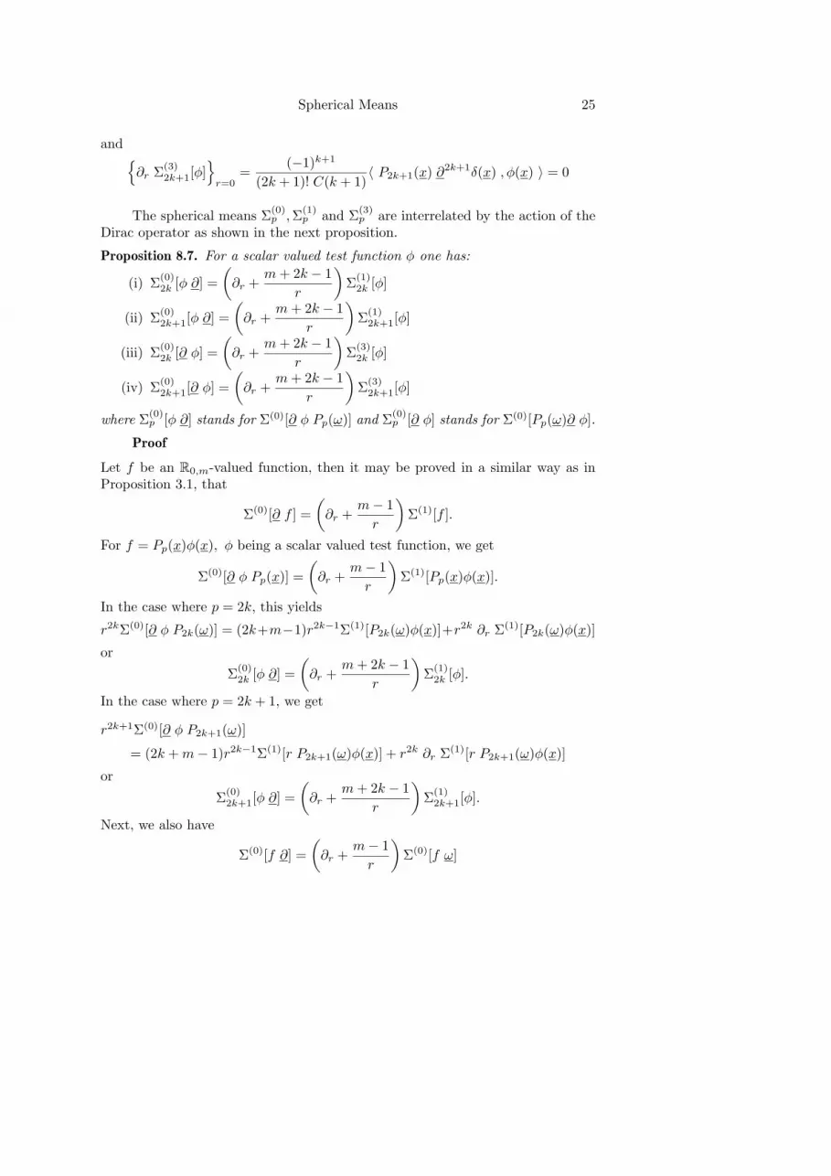
Spherical Means 25

and∂r Σ

(3)2k+1[φ]

r=0=

(−1)k+1

(2k + 1)! C(k + 1)〈 P2k+1(x) ∂

2k+1δ(x) , φ(x) 〉 = 0

The spherical means Σ(0)p ,Σ

(1)p and Σ

(3)p are interrelated by the action of the

Dirac operator as shown in the next proposition.

Proposition 8.7. For a scalar valued test function φ one has:

(i) Σ(0)2k [φ ∂] =

(∂r +

m+ 2k − 1

r

)Σ

(1)2k [φ]

(ii) Σ(0)2k+1[φ ∂] =

(∂r +

m+ 2k − 1

r

)Σ

(1)2k+1[φ]

(iii) Σ(0)2k [∂ φ] =

(∂r +

m+ 2k − 1

r

)Σ

(3)2k [φ]

(iv) Σ(0)2k+1[∂ φ] =

(∂r +

m+ 2k − 1

r

)Σ

(3)2k+1[φ]

where Σ(0)p [φ ∂] stands for Σ(0)[∂ φ Pp(ω)] and Σ

(0)p [∂ φ] stands for Σ(0)[Pp(ω)∂ φ].

Proof

Let f be an R0,m-valued function, then it may be proved in a similar way as inProposition 3.1, that

Σ(0)[∂ f ] =

(∂r +

m− 1

r

)Σ(1)[f ].

For f = Pp(x)φ(x), φ being a scalar valued test function, we get

Σ(0)[∂ φ Pp(x)] =

(∂r +

m− 1

r

)Σ(1)[Pp(x)φ(x)].

In the case where p = 2k, this yields

r2kΣ(0)[∂ φ P2k(ω)] = (2k+m−1)r2k−1Σ(1)[P2k(ω)φ(x)]+r2k ∂r Σ(1)[P2k(ω)φ(x)]

or

Σ(0)2k [φ ∂] =

(∂r +

m+ 2k − 1

r

)Σ

(1)2k [φ].

In the case where p = 2k + 1, we get

r2k+1Σ(0)[∂ φ P2k+1(ω)]

= (2k +m− 1)r2k−1Σ(1)[r P2k+1(ω)φ(x)] + r2k ∂r Σ(1)[r P2k+1(ω)φ(x)]

or

Σ(0)2k+1[φ ∂] =

(∂r +

m+ 2k − 1

r

)Σ

(1)2k+1[φ].

Next, we also have

Σ(0)[f ∂] =

(∂r +

m− 1

r

)Σ(0)[f ω]


which, for f = Pp(x)φ(x), turns into

Σ(0)[Pp(x) ∂ φ] =

(∂r +

m− 1

r

)Σ(0)[Pp(x) ω φ(x)].

In the case where p = 2k, this yields:

r2k Σ(0)[P2k(ω) ∂φ]

= (2k +m− 1)r2k−1 Σ(0)[P2k(ω) ω φ(x)] + r2k ∂r Σ(0)[P2k(ω) ω φ(x)]

or

Σ(0)2k [∂ φ] =

(∂r +

m+ 2k − 1

r

)Σ

(3)2k [φ].

In the case where p = 2k + 1, we get

r2k+1Σ(0)[P2k+1(ω) ∂ φ] = (2k +m− 1)r2k−1 Σ(0)[r P2k+1(ω) ω φ(x)]

+ r2k ∂r Σ(0)[r P2k+1(ω) ω φ(x)]

or

Σ(0)2k+1[∂ φ] =

(∂r +

m+ 2k − 1

r

)Σ

(3)2k+1[φ].

Proposition 8.8. For a scalar valued test function φ one has:

(i) r Σ(1)2k [φ ∂] =

r

am

∫

Sm−1

∂ φ ω P2k(ω) dS(ω) =

(−r ∂r + 2k)Σ(0)2k [φ]

(ii) r Σ(1)2k+1[φ ∂] =

r2

am

∫

Sm−1

∂ φ ω P2k+1(ω) dS(ω) =

(−r ∂r + 2k + 2)Σ(0)2k+1[φ]

(iii) r Σ(3)2k [∂ φ] =

r

am

∫

Sm−1

P2k(ω) ω ∂ φ dS(ω) =

(−r ∂r + 2k)Σ(0)2k [φ]

(iv) r Σ(3)2k+1[∂ φ] =

r2

am

∫

Sm−1

P2k+1(ω) ω ∂ φ dS(ω) =

(−r ∂r + 2k + 2)Σ(0)2k+1[φ]

The proof is similar to that of Proposition 8.7.

Spherical Means 27

9. New Clifford distributions

The technique used in this section for introducing new Clifford distributions is es-sentially the same as in the first part of this paper; we use spherical co-ordinates,the fundamental distribution Fpr

µ+ and the new spherical means of the foregoing

section 8.

Let λ be a complex parameter and let φ be a scalar valued test funtion.

We define the vector valued distributions Tλ,p by:

〈 Tλ,2k, φ 〉 = am 〈 Fp rµ+2k+ ,Σ

(0)2k [φ] 〉

and

〈 Tλ,2k+1, φ 〉 = am 〈 Fp rµ+2k+ ,Σ

(0)2k+1[φ] 〉

where we have put

µ = λ+m− 1

In the same order of ideas as in part I, we also introduce the distributionsUλ,p and Vλ,p by:

〈 Uλ,2k, φ 〉 = am〈 Fp rµ+2k+ ,Σ

(1)2k [φ] 〉

〈 Uλ,2k+1, φ 〉 = am〈 Fp rµ+2k+ ,Σ

(1)2k+1[φ] 〉

〈 Vλ,2k, φ 〉 = am〈 Fp rµ+2k+ ,Σ

(3)2k [φ] 〉

〈 Vλ,2k+1, φ 〉 = am〈 Fp rµ+2k+ ,Σ

(3)2k+1[φ] 〉

Example 9.1. For λ = −m− p, we have for p = 2k:

〈 T−m−2k,2k, φ 〉 = am〈 Fp r−1+ ,Σ

(0)2k [φ] 〉

=

∫ +∞

0

1

rdr

∫

Sm−1

P2k(ω) φ(x) dS(ω)

=

∫

Rm

1

rmP2k(ω)[φ(x)− φ(0)] dV (x)

= limε→

>0

∫

Rm\B(0,ε)

1

rmP2k(ω) φ(x) dV (x)

where we have used the fact (see Remark 8.3) that∫

Sm−1

P2k(ω) dS(ω) = 0

Similarly we obtain for p = 2k + 1 that

〈 T−m−2k−1,2k+1, φ 〉 = limε→

>

∫

Rm\B(0,ε)

1

rmP2k+1(ω) φ(x) dV (x)


The distribution T−m−p,p thus turns out to be a so-called principal value distribu-

tion (see [9]):

T−m−p,p = PvPp(ω)

rm

which yields another example of a convolution operator (see also 6.2).

In the same order of ideas we find

U−m−p,p = Pvω Pp(ω)

rm

and

V−m−p,p = PvPp(ω) ω

rm

to be examples of such kind of distributions. Moreover we have

Pvω Pp(ω)

rm+ Pv

Pp(ω) ω

rm= −2(p+ 1) Pv

Sp+1(ω)

rm

showing that the U−m−p,p and V−m−p,p distributions may be used for decomposingthe scalar valued principal value distribution Pv 1

rm Sp+1(ω) of [9] and [12].

Other examples of the Tλ,p, Uλ,p and Vλ,p distributions are given in thesections 10 and 11.

10. The action of the Dirac operator on the distributions Tλ,p

We expect the distributions Tλ,p, Uλ,p and Vλ,p to be interrelated by the action ofthe Dirac operator. As Tλ,p is vector valued, it makes sense to distinguish betweenan action of ∂ from the left or from the right.As it is clear that the parity of the degree p of the spherical monogenic Pp influencesthe calculations and the results, we introduce the notation pe (”even part of p”)by

pe = 2k if p = 2kpe = 2k if p = 2k + 1

In a series of propositions we summarize the results of the calculations of ∂ Tλ,pand Tλ,p ∂ in the several cases to be distinguished; their proofs are similar to that

of Proposition 5.1. Note that, as the odd order derivatives of Σ(0)p [φ] vanish at

r = 0, we have to expect a singular term involving odd order derivatives of thedelta distribution, only if λ+m+ pe is even.

Proposition 10.1. For λ ∈ C and p ∈ N such that λ+m−1+pe 6= 0,−1,−2,−3, . . .one has

∂ Tλ,p = λ Uλ−1,p

and

Tλ,p ∂ = λ Vλ−1,p

Spherical Means 29

Example 10.2. Take λ+ 2k = 0; then µ+ pe = m− 1 and

〈 T−2k,2k, φ 〉 = am〈 Fp rm−1+ , Σ

(0)2k [φ] 〉

=

∫ +∞

0

rm−1 dr

∫

Sm−1

P2k(ω)φ(x) dS(ω)

=

∫

Rm

P2k(ω)φ(x) dV (x)

whence

T−2k,2k(x) = P2k(ω)

If λ+ 2k + 1 = 0 then µ+ pe = m− 2 and

〈 T−2k−1,2k+1, φ 〉 = am〈 Fp rm−2+ , Σ

(0)2k+1[φ] 〉

=

∫ +∞

0

rm−2 dr

∫

Sm−1

P2k+1(ω)φ(x) dS(ω)

=

∫

Rm

P2k+1(ω)φ(x) dV (x)

whence

T−2k−1,2k+1(x) = P2k+1(ω)

In a similar way it is shown that

U−p−1,p(x) =1

rω Pp(ω)

and

V−p−1,p(x) =1

rPp(ω)ω

By Proposition 10.1 we get:

∂ T−p,p (x) = (−p) U−p−1,p(x)

and

T−p,p ∂ = (−p) V−p−1,p(x)

or thus

∂ Pp(ω) = (−p)1

rω Pp(ω)

and

Pp(ω) ∂ = (−p)1

rPp(ω) ω

confirming known formulae (see section 7).

Proposition 10.3. For λ ∈ C and p ∈ N such that λ+m− 1 + pe = 0 one has

∂ T−m+1−pe,p = −(m+ pe − 1)U−m−pe,p

and

T−m+1−pe,p ∂ = −(m+ pe − 1)V−m−pe,p


Remark 10.4. The distribution considered in the above proposition is, by defini-tion:

〈 T−m−2k+1,2k(x), φ(x) 〉 = am〈 Fp r0+,Σ(0)2k [φ] 〉

=

∫ +∞

0

dr

∫

Sm−1

P2k(ω)φ(r ω) dS(ω) =

∫

Rm

1

rm−1P2k(ω) φ(x) dV (x)

whence

T−m−2k+1,2k(x) =1

rm−1P2k(ω)

and similarly

T−m−2k+1,2k+1(x) =1

rm−2P2k+1(ω)

which are clearly locally integrable functions in Rm.

We also have

〈 φ, U−m−2k,2k(x) 〉 = am〈 Fp r−1+ ,Σ

(1)2k [φ] 〉

and hence

U−m−2k,2k(x) = Fp1

rmω P2k(ω) = Pv

ω P2k(ω)

rm

and similarly

U−m−2k,2k+1(x) =1

rm−1ω P2k+1(ω) = am Em(x) P2k+1(ω)

The formulae of Proposition 10.3 may thus be rewritten as:

∂

(1

rm−1P2k(ω)

)= (m+ 2k − 1) Pv

ω

rmP2k(ω)

and

∂

(1

rm−2P2k+1(ω)

)= −(m+ 2k − 1) am Em(x) P2k+1(ω)

Proposition 10.5. For λ ∈ C and p ∈ N such that λ+m−1+pe = −s, s = 1, 2, 3, . . .one has

(i) ∂ T−m+1−2k−2l,2k = −(m+ 2k + 2l − 1) U−m−2k−2l,2k, l = 1, 2, 3, . . .

(ii) ∂ T−m−2k−2l,2k = −(m+ 2k + 2l) U−m−2k−2l−1,2k

+am(−1)k+l+1 (∂2k+2l+1δ(x))P2k(x)

(2k + 2l + 1)!C(k + l + 1), l = 0, 1, 2, 3, . . .

(iii) ∂ T−m+1−2k−2l,2k+1 = −(m+ 2k + 2l − 1) U−m−2k−2l,2k+1, l = 1, 2, 3, . . .

(iv) ∂ T−m−2k−2l,2k+1 = −(m+ 2k + 2l) U−m−2k−2l−1,2k+1

+am(−1)k+l+1 (∂2k+2l+1δ(x))P2k+1(x)

(2k + 2l + 1)!C(k + l + 1), l = 0, 1, 2, 3, . . .

Spherical Means 31

and similar formulae for Tλ,p ∂.

11. The action of the Dirac operator on the distributions Uλ,p andVλ,p

In this section we study the action of the Dirac operator from the left on Uλ,p

considered as a left distribution, and the action from the right on Vλ,p consideredas a right distribution. For the action of the Dirac operator from the right on Uλ,p

and from the left on Vλ,p, we refer the reader to [3] which is a continuation of thepresent paper.It turns out that the mentioned action of the Dirac operator reproduces – in thegeneral case – the distributions Tλ−1,p .The proofs of the following propositionsare similar to that of Proposition 5.2. Note that, as the even order derivatives of

Σ(1)p [φ] and Σ

(3)p [φ] vanish at r = 0, we have to expect a singular term involving

even order derivatives of the delta distribution, only if λ+m+ pe is odd.

Proposition 11.1. For λ ∈ C and p ∈ N such that λ+m−1+pe 6= 0,−1,−2,−3, . . .one has:

∂ Uλ,2k = Vλ,2k ∂ = −(λ+m− 1 + 4k) Tλ−1,2k

and

∂ Uλ,2k+1 = Vλ,2k+1 ∂ = −(λ+m+ 1 + 4k) Tλ−1,2k+1

Example 11.2. We verify the formulae of Proposition 11.1 in the specific casewhere, for λ = 1, we have:

U1,p = rp+1 ω Pp(ω)

The left hand side of the formula then takes the form:

∂ U1,p = −(m+ 2p) rp Pp(ω)

while on the right hand side we have for p = 2k:

−(λ+m− 1 + 4k) Tλ−1,2k = −(m+ 4k) T0,2k = −(m+ 4k) r2k P2k(ω)

and for p = 2k + 1:

−(λ+m+1+4k) Tλ−1,2k+1 = −(m+4k+2) T0,2k+1 = −(m+4k+2) r2k+1 P2k+1(ω)

Example 11.3. Take λ = −2k and p = 2k; then µ+ pe = m− 1 and

〈 U−2k,2k, φ 〉 = am〈 Fp rm−1+ ,Σ

(1)2k [φ] 〉

=

∫ +∞

0

rm−1 dr

∫

Sm−1

ω P2k(ω) φ(x) dS(ω)

whence

U−2k,2k(x) = ω P2k(ω)


If λ = −2k − 1 and p = 2k + 1, then µ+ pe = m− 2 and

〈 U−2k−1,2k+1, φ 〉 = am〈 Fp rm−2+ ,Σ

(1)2k+1[φ] 〉

=

∫ +∞

0

rm−2 dr

∫

Sm−1

r ω P2k+1(ω) φ(x) dS(ω)

whence

U−2k−1,2k+1 = ω P2k+1(ω)

We thus obtain in this specific case the left and right outer spherical monogenics(see section 7):

U−p,p = ω Pp(ω) = Q(l)p (ω)

and

V−p,p = Pp(ω) ω = Q(r)p (ω)

The formulae of Proposition 11.1 yield:

∂ U−2k,2k = V−k,2k ∂ = −(m+ 2k − 1) T−2k−1,2k

and

∂ U−2k−1,2k+1 = V−2k−1,2k+1 ∂ = −(m+ 2k) T−2k−2,2k+1

or, in terms of the outer spherical monogenics:

∂(ω P2k(ω)) = (P2k(ω) ω)∂ = −(m+ 2k − 1)1

rP2k(ω)

and

∂(ω P2k+1(ω)) = (P2k+1(ω) ω)∂ = −(m+ 2k)1

rP2k+1(ω)

in accordance with the formulae of section 7.

Proposition 11.4. For λ ∈ C and p ∈ N such that λ+m− 1 + pe = 0 one has:

∂ U−m−2k+1,2k = V−m−2k+1,2k ∂

= −2k T−m−2k,2k − am1

(2k)!

1

C(k)P2k(x) ∆

km δ(x)

and

∂ U−m−2k+1,2k+1 = V−m−2k+1,2k+1 ∂

= −(2k + 2) T−m−2k,2k+1 − am1

(2k)!

1

C(k)P2k+1(x) ∆

km δ(x)

Proposition 11.5. For λ ∈ C and p ∈ N such that λ+m− 1 + pe = −s,s = 1, 2, 3, . . . one has:

∂ U−m−2k−2l+1,2k =

(2l − 2k) T−m−2k−2l,2k

−am1

(2k + 2l)!

1

C(k + l)P2k(x) ∆

k+lm δ(x), l = 1, 2, 3, . . .

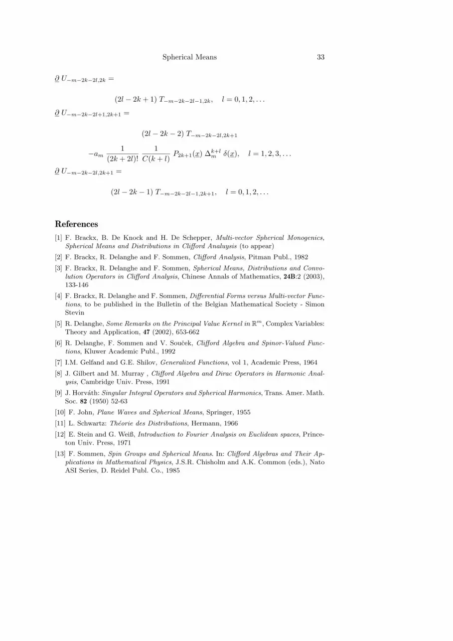
Spherical Means 33

∂ U−m−2k−2l,2k =

(2l − 2k + 1) T−m−2k−2l−1,2k, l = 0, 1, 2, . . .

∂ U−m−2k−2l+1,2k+1 =

(2l − 2k − 2) T−m−2k−2l,2k+1

−am1

(2k + 2l)!

1

C(k + l)P2k+1(x) ∆

k+lm δ(x), l = 1, 2, 3, . . .

∂ U−m−2k−2l,2k+1 =

(2l − 2k − 1) T−m−2k−2l−1,2k+1, l = 0, 1, 2, . . .

References

[1] F. Brackx, B. De Knock and H. De Schepper, Multi-vector Spherical Monogenics,

Spherical Means and Distributions in Clifford Analuysis (to appear)

[2] F. Brackx, R. Delanghe and F. Sommen, Clifford Analysis, Pitman Publ., 1982

[3] F. Brackx, R. Delanghe and F. Sommen, Spherical Means, Distributions and Convo-

lution Operators in Clifford Analysis, Chinese Annals of Mathematics, 24B:2 (2003),133-146

[4] F. Brackx, R. Delanghe and F. Sommen, Differential Forms versus Multi-vector Func-

tions, to be published in the Bulletin of the Belgian Mathematical Society - SimonStevin

[5] R. Delanghe, Some Remarks on the Principal Value Kernel in Rm, Complex Variables:

Theory and Application, 47 (2002), 653-662

[6] R. Delanghe, F. Sommen and V. Soucek, Clifford Algebra and Spinor-Valued Func-

tions, Kluwer Academic Publ., 1992

[7] I.M. Gelfand and G.E. Shilov, Generalized Functions, vol 1, Academic Press, 1964

[8] J. Gilbert and M. Murray , Clifford Algebra and Dirac Operators in Harmonic Anal-

ysis, Cambridge Univ. Press, 1991

[9] J. Horvath: Singular Integral Operators and Spherical Harmonics, Trans. Amer. Math.Soc. 82 (1950) 52-63

[10] F. John, Plane Waves and Spherical Means, Springer, 1955

[11] L. Schwartz: Theorie des Distributions, Hermann, 1966

[12] E. Stein and G. Weiß, Introduction to Fourier Analysis on Euclidean spaces, Prince-ton Univ. Press, 1971

[13] F. Sommen, Spin Groups and Spherical Means. In: Clifford Algebras and Their Ap-

plications in Mathematical Physics, J.S.R. Chisholm and A.K. Common (eds.), NatoASI Series, D. Reidel Publ. Co., 1985


Ghent University, Department of Mathematical Analysis, B-9000 Gent, BelgiumE-mail address: [email protected]

E-mail address: [email protected]

E-mail address: [email protected]

Documents

Spherical Means and Distributions in Clifford Analysis