Spitzer SAGE Survey of the Large Magellanic Cloud. II. Evolved Stars and Infrared Color-Magnitude Diagrams

The Astronomical Journal, 136:18–43, 2008 July doi:10.1088/0004-6256/136/1/18c© 2008. The American Astronomical Society. All rights reserved. Printed in the U.S.A.

SPITZER SAGE SURVEY OF THE LARGE MAGELLANIC CLOUD. III. STAR FORMATION AND ∼1000 NEWCANDIDATE YOUNG STELLAR OBJECTS

B. A. Whitney1, M. Sewilo2, R. Indebetouw3, T. P. Robitaille4, M. Meixner2, K. Gordon5, M. R. Meade6, B. L. Babler6,J. Harris5, J. L. Hora7, S. Bracker6, M. S. Povich6, E. B. Churchwell6, C. W. Engelbracht5, B-Q For5,8, M. Block5,K. Misselt5, U. Vijh2, C. Leitherer2, A. Kawamura9, R. D. Blum10, M. Cohen11, Y. Fukui9, A. Mizuno9, N. Mizuno9,

S. Srinivasan12, A. G. G. M. Tielens13, K. Volk14, J-P. Bernard15, F. Boulanger16, J. A. Frogel17, J. Gallagher6,V. Gorjian18, D. Kelly5, W. B. Latter19, S. Madden20, F. Kemper21, J. R. Mould10, A. Nota2, M. S. Oey22, K. A. Olsen23,

T. Onishi9, R. Paladini24, N. Panagia2, P. Perez-Gonzalez5, W. Reach24, H. Shibai9, S. Sato9, L. J. Smith2,25,L. Staveley-Smith26, T. Ueta27, S. Van Dyk24, M. Werner18, M. Wolff1, and D. Zaritsky5

1 Space Science Institute, 4750 Walnut St. Suite 205, Boulder, CO 80301, USA; [email protected], [email protected] Space Telescope Science Institute, 3700 San Martin Way, Baltimore, MD 21218, USA; [email protected], [email protected], [email protected], [email protected],

[email protected], [email protected], and [email protected] Department of Astronomy, University of Virginia, P.O. Box 3818, Charlottesville, VA 22903, USA; [email protected]

4 School of Physics and Astronomy, University of St Andrews, North Haugh, KY16 9SS, St Andrews, UK; [email protected] Steward Observatory, University of Arizona, 933 North Cherry Ave., Tucson, AZ 85719, USA; [email protected], [email protected],

[email protected], [email protected], [email protected], [email protected], [email protected], [email protected]

6 Department of Astronomy, 475 North Charter St., University of Wisconsin, Madison, WI 53706, USA; [email protected], [email protected],[email protected], [email protected], [email protected], and [email protected]

7 Center for Astrophysics, 60 Garden St., MS 67, Harvard University, Cambridge, MA 02138, USA; [email protected] Department of Astronomy, University of Texas at Austin, 1 University Station, C1400, Austin, TX 78712, USA; [email protected]

9 Department of Astrophysics, Nagoya University, Chikusa-ku, Nagoya 464-8602, Japan; [email protected], [email protected],[email protected], [email protected], [email protected], [email protected], and [email protected]

10 NOAO, P.O. Box 26732, Tucson AZ 85726-6732, USA; [email protected], [email protected] Radio Astronomy Laboratory, 601 Campbell Hall, University of California at Berkeley, Berkeley, CA 94720, USA; [email protected]

12 Department of Physics and Astronomy, Johns Hopkins University, Homewood Campus, Baltimore, MD 21218, USA; [email protected] NASA Ames Research Center, SOFIA Office, MS 211-3, Moffet Field, CA 94035, USA; [email protected]

14 Gemini Observatory, 670 North A’ohuku Place, Hilo, HI 96720, USA; [email protected] Centre d’ Etude Spatiale des Rayonnements, CNRS, 9 av. du Colonel Roche, BP 4346, 31028 Toulouse, France; [email protected]

16 Astrophysique de Pari, Institute (IAP), CNRS UPR 341, 98bis, Boulevard Arago, Paris, F-75014, France; [email protected] AURA, Inc., 1200 New York Ave. NW, Suite 350, Washington D.C. 20005, USA; [email protected]

18 Jet Propulsion Lab, 4800 Oak Grove Dr., MS 264–767, Pasadena, CA 91109, USA; [email protected], [email protected] Caltech, NASA Herschel Science Center, MS 100–22, Pasadena, CA 91125, USA; [email protected]

20 Service dAstrophysique CEA, Saclay, 91191 Gif Sur Yvette Cedex, France; [email protected] Jodrell Bank Centre for Astrophysics, University of Manchester, M13 9PL, Manchester, UK; [email protected] Department of Astronomy, University of Michigan, 830 Dennison Bldg., Ann Arbor, MI 48109, USA; [email protected]

23 Cerro Tololo Interamerican Observatory, Casilla 603, La Serena, Chile; [email protected] Spitzer Science Center, California Institute of Technology, 220-6, Pasadena, CA, 91125, USA; [email protected], [email protected]

25 Department of Physics and Astronomy, University College London, Gower Street, London WC1E 6BT, UK26 Australia Telescope National Facility, CSIRO, P.O. Box 76, Epping NSW 1710, Australia; [email protected]

27 Department of Physics and Astronomy, University of Denver, Denver, CO 80208, USA; [email protected] 2007 June 20; accepted 2008 April 1; published 2008 May 27

ABSTRACT

We present ∼1000 new candidate Young Stellar Objects (YSOs) in the Large Magellanic Cloud selected fromSpitzer Space Telescope data, as part of the Surveying the Agents of a Galaxy’s Evolution (SAGE) Legacy program.The YSOs, detected by their excess infrared (IR) emission, represent early stages of evolution, still surroundedby disks and/or infalling envelopes. Previously, fewer than 20 such YSOs were known. The candidate YSOswere selected from the SAGE Point Source Catalog from regions of color–magnitude space least confused withother IR-bright populations. The YSOs are biased toward intermediate- to high-mass and young evolutionarystages, because these overlap less with galaxies and evolved stars in color–magnitude space. The YSOs are highlycorrelated spatially with atomic and molecular gas, and are preferentially located in the shells and bubbles createdby massive stars inside. They are more clustered than generic point sources, as expected if star formation occursin filamentary clouds or shells. We applied a more stringent color–magnitude selection to produce a subset of“high-probability” YSO candidates. We fitted the spectral-energy distributions (SEDs) of this subset and derivedphysical properties for those that were well fitted. The total mass of these well-fitted YSOs is ∼2900 M� and thetotal luminosity is ∼2.1 × 106L�. By extrapolating the mass function with a standard initial mass function andintegrating, we calculate a current star-formation rate of ∼0.06 M� yr−1, which is at the low end of estimatesbased on total ultraviolet and IR flux from the galaxy (∼0.05 − 0.25 M� yr−1), consistent with the expectationthat our current YSO list is incomplete. Follow-up spectroscopy and further data mining will better separate thedifferent IR-bright populations and likely increase the estimated number of YSOs. The full YSO list is available aselectronic tables, and the SEDs are available as an electronic figure for further use by the scientific community.

Key words: circumstellar matter – galaxies: dwarf – infrared: stars – Magellanic Clouds – stars: formation – stars:pre-main sequence

Online-only material: extended figure set, machine-readable and VO tables

18

http://dx.doi.org/10.1088/0004-6256/136/1/18

mailto:[email protected]






















































No. 1, 2008 SPITZER SAGE SURVEY OF THE LMC. III. 19

1. INTRODUCTION

The Large Magellanic Cloud (LMC) holds an advantageousposition for studying extragalactic star formation. Its proximity,50 kpc (e.g., Panagia 2005), permits individual Young Stel-lar Objects (YSOs) to be identified with the <2′′(<0.5 pc)resolution available in the optical and near-infrared (IR) us-ing ground-based telescopes, and now in the mid-IR with theSpitzer Space Telescope (Werner et al. 2004). The favorableviewing angle of this flattened galaxy (35◦, van der Marel &Cioni 2001) limits line-of-sight confusion and allows correla-tion of the YSOs with the interstellar medium (ISM) clouds.The LMC may provide insight into the star-formation processesduring the epoch of peak star formation in the universe (red-shift of ∼1.5, Madau et al. 1996) because the LMC’s metal-licity (Z ∼ 0.3 − 0.5Z�; Westerlund 1997) is similar to themean metallicity of the universe at redshift of ∼1.5 (e.g., Peiet al. 1999). In addition to its value in studying extragalacticstar formation, star formation in the LMC is in some wayseasier to study than in our own Galaxy since the distancesto the YSOs are known. In the following, we highlight some ofthe previous findings on star formation in the LMC and how theSpitzer Surveying the Agents of a Galaxy’s Evolution (SAGE)IR survey (Meixner et al. 2006) can contribute new information:

1. The star-formation history of the LMC can be determinedby modeling optical color–magnitude diagrams (CMDs)obtained from telescopes (e.g., the Hubble Space Telescope(HST)) that can resolve individual stars (e.g., Gallagheret al. 1996; Olsen 1999; Smecker-Hane et al. 2002). Fromsuch studies, we have learned that the disk star-formationrate (SFR) has been relatively constant over the last ∼15Gyr, while the bar star formation has been much moreepisodic. Studies of clusters have shown that the LMCappears to be in an active epoch of cluster formation, whichbegan about 3–4 Gyr ago (Da Costa 1991; Hodge 1988).During this time, the SFR has increased by a factor ofabout 3 (Geha et al. 1998; Holtzman et al. 1997). Thesestudies nicely determine histories and relative rates of starformation. High-resolution IR studies can complement thiswork by determining the current SFR.

2. The correlation of giant molecular clouds (Fukui et al. 1999,from the NANTEN CO survey) to optical clusters (e.g.,Bica et al. 1996) suggests that the clouds are short lived.This is based on the fact that about half of the CO cloudsare associated with the youngest stellar activity (<10 Myrclusters and H ii regions), implying that stellar clusters areactively formed over about 50% of the cloud lifetime andthat the clouds are dissipated on timescales of ∼6 Myr.Additionally, the CO and ultraviolet emission are spatiallyanti-correlated, suggesting that stellar photons disrupt theclouds. A complete census of YSOs can shed further lighton these issues by the degree to which YSOs are spatiallycorrelated with ultraviolet and CO emission. If molecularcloud lifetimes are short, the efficiency of star formationover the short lifetime must be high to obtain a time- andspatially-averaged efficiency of ∼1%. Thus, we should ex-pect to see star formation occurring in most of the molecularclouds, as is the case in the solar neighborhood (Hartmannet al. 2001). Twelve of the 55 well-studied molecular cloudsshow no star-formation activity, based on optical and near-IR observations (Fukui et al. 1999). A mid-IR survey canreveal more deeply embedded star formation not seen inthe near-IR, through both increased emission and decreased

extinction, and can more accurately determine the percent-ages of molecular clouds that are forming stars.

3. Targeted high-spatial-resolution optical and near-IR ob-servations with HST have identified populations of likelypre-main-sequence (MS) stars based on large reddeningor near-IR excesses (Walborn et al. 1999; Panagia et al.2000; Romaniello et al. 2006; Gouliermis et al. 2006).Two of the most well-studied regions in the LMC are 30Doradus (N157), and the N159/N160 region just south ofit. Brandner et al. (2001) present NICMOS near-IR imag-ing in the filaments near R136 in the 30 Doradus region,mostly pointed at previously identified candidate protostel-lar objects and knots of star formation (Hyland et al. 1992;Rubio et al. 1992, among others). They identify 24 candi-date protostars, including new, faint sources whose lumi-nosities and colors are consistent with T Tauri stars. Thedistribution of young sources in the compressed molecularridge north of R136 supports a model of triggered star for-mation in this region. LMC star formation may in general beself-propagating through the energetic feedback of stellarwinds and supernovae (e.g., Oey & Massey 1995; Efremov& Elmegreen 1998a) but this stellar feedback also acts toeventually squelch star formation by dissipating the localISM (Yamaguchi et al. 2001; Israel et al. 2003). The SAGEIR survey provides a global picture of star formation in theLMC, and can determine if star formation occurs in clustersand supershells, and the importance of local triggering andself-propagation.

4. Star formation in the LMC is likely influenced by itsinteractions with its neighbors. Recent HST observations ofproper motions in the LMC (Kallivayalil et al. 2006b) andSmall Magellanic Cloud (SMC) (Kallivayalil et al. 2006a)suggest that the 3D velocities of the Clouds are much higherthan previously thought, and the Clouds are on their firstpassage through the Milky Way (Besla et al. 2007). Beslaet al. (2007) suggest that the rise in the SFR in the past 3 Gyr(Zaritsky & Harris 2004) is due to tidal forces as the Cloudsapproached the Galactic center. It has been proposed thatthe southeastern arc in the LMC is star formation triggeredby the bow shock as the LMC travels through the MilkyWay halo (e.g., de Boer et al. 1998). An IR census canaddress whether the current global rate of star formationis consistent with an enhancement caused by the currentperiGalactic passage.

Current star formation is most directly studied with IR in-strumentation, since stars form from collapsing dusty envelopeswhich reradiate the absorbed short-wavelength emission at IRwavelengths. Previous large-scale mid-IR surveys have beenlimited by resolution and sensitivity. The IRAS survey can beused to identify regions of massive star formation but the low-spatial-resolution makes it difficult to characterize the regionsand to tell protostars from the associated diffuse ionized gas, ne-cessitating follow-up at 1 arcsec or better resolution. For exam-ple, Indebetouw et al. (2004) mapped the compact H ii regionsusing centimeter-wave interferometry, separating them fromembedded YSOs. While Midcourse Space Experiment (MSX)8 µm maps of the LMC provided a wealth of new informationon the IR population of the LMC (Egan et al. 2001), MSX Eband (21 µm) sensitivity was insufficient to image any but thebrightest regions in the Magellanic Clouds.

The Spitzer SAGE project (Meixner et al. 2006) allows forthe first time a global study of star formation in the LMC at highenough resolution to resolve individual cores and protostars at a

20 WHITNEY ET AL. Vol. 136

range of mid-IR wavelengths. SAGE is a Legacy project on theSpitzer Space Telescope (Werner et al. 2004), which mapped a7◦ × 7◦ region of the LMC using the IRAC camera in the 3.6,4.5, 5.8, and 8.0 µm filters (Fazio et al. 2004) and the MIPScamera in the 24, 70, and 160 µm filters (Rieke et al. 2004).The survey was done over two epochs with a total observingtime of 291 hr with IRAC and 217 hrs with MIPS. The detailsof the survey are described in Meixner et al. (2006).28 In thispaper, we use the SAGE first epoch Point Source Catalogs ofIRAC and MIPS 24 µm that have been merged together withTwo Micron All Sky Survey (2MASS) JHKs (1.2, 1.6, and2.2 µm) (Skrutskie et al. 2006).

This paper presents a selection of ∼1000 YSO candidateschosen from the SAGE Point Source Catalog based on theirIR colors and magnitudes. The current list is incomplete onboth the low- and high-mass ends, but should provide a richdataset for follow-up observations. The candidate YSO list isavailable as an online table, as is a table of estimated physicalproperties of selected YSOs, and an electronic figure of all of thespectral-energy distributions (SEDs). In Section 2 we describeour selection method for the YSOs. Section 3 discusses theirproperties and comparisons to previously known YSOs, andSection 4 summarizes the results.

2. COLOR–MAGNITUDE SELECTION OF YOUNGSTELLAR OBJECTS

One advantage of studying star formation in the LMCcompared to large regions of the Galaxy is that the distanceis known and we can use the magnitude in addition to colorsto separate YSOs from other populations. In this section wedescribe our method for selecting the YSOs. We first describewhere we expect YSOs to lie in color–magnitude space basedon radiation transfer models (Section 2.1). Next we describethe SAGE Catalog from which the YSOs will be selected, andidentify known populations such as galaxies and evolved starsin the CMDs (Section 2.2). Finally, in Section 2.3 we describethe color–magnitude selection of the YSOs, and further cullingand quality checks.

2.1. The Expected Colors and Magnitudes of YSOs

YSOs are typically surrounded by dusty envelopes and disks.In their early stages of evolution, the envelopes are opaque andrelatively cool, and absorb most of the central stellar radiation,re-emitting in the IR at the temperature of the dust. As thesesources evolve, the envelopes and disks disperse and emit lessIR radiation. An ensemble of YSOs of different evolutionarystages and masses will span a large range in IR colors. Robitailleet al. (2006) computed a grid of 20,000 2D radiation transfermodels intended to cover the full range of stellar masses andevolutionary stages of YSOs. Each model produces SEDs at teninclinations and 50 apertures. The models accurately computescattered and thermal emission from dust in a physicallyplausible geometry, which consists of a stellar source thatilluminates a dusty disk, envelope, and bipolar cavity (Whitneyet al. 2003a, 2003b). The models are based on observationsand theory of known Galactic star-forming regions, and havebeen used to fit SEDs of YSOs in the Taurus molecular cloud(Robitaille et al. 2007), the G34.4+0.2 massive star-forming

28 Catalogs that combine 2MASS JHKs , IRAC and MIPS 24 are available atthe Spitzer Science Center Websitehttp://ssc.spitzer.caltech.edu/legacy/all.html.

region (Shepherd et al. 2007), the M16 star-forming region(Indebetouw et al. 2007), several newly discovered massiveYSOs formed in bubbles (Watson et al. 2008), as well as YSOsin the SMC (Simon et al. 2007).

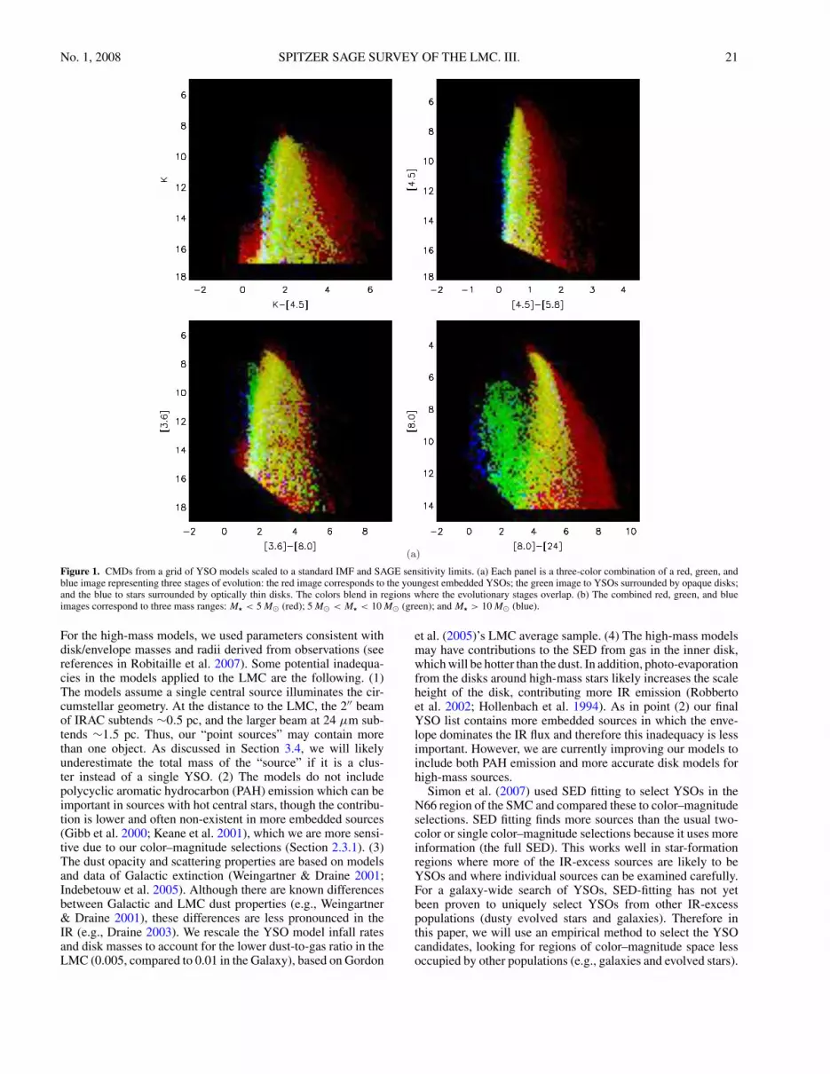
We can use the grid of models to estimate where the LMCYSOs might lie in color–magnitude space. As described inRobitaille et al. (2006), we can create a model CMD of theLMC by weighting models of the grid to produce a standardInitial Mass Function (IMF) for the stellar masses (Kroupa2001), and a constant SFR beginning two million years ago.Most of the YSOs we are sensitive to will be much youngerthan this and thus there is no need to go further back in time.We define the age of a source as the time since the pre-MScontraction began. For the IMF, we use average slopes of −1.3for stellar mass greater than 0.5, and −0.3 for mass less than0.5 and a mass range of 0.08–50 M� (Kroupa 2001). We thenscaled the resulting model fluxes to the distance of the LMC andapplied the same sensitivity limits as the SAGE data. A similarcomparison of our model CMDs and CCDs in the Perseus star-formation region found good agreement between the modelsand data (Harvey et al. 2007). The resulting distribution ofmodel YSOs is shown in Figure 1. The CMDs are displayedas Hess diagrams (2D histograms where the number density isrepresented by the brightness of each pixel), but in three colors.The models were divided into three ranges of evolutionary stage(Figure 1(a)) and mass bins (Figure 1(b)). In Figure 1(a), the redimage in each panel corresponds to the youngest YSOs (Stage I:embedded in an infalling envelope); the green image to starssurrounded by opaque disks (Stage II); and blue to starssurrounded by optically thin disks (Stage III). The stages weredefined in Robitaille et al. (2006) based on comparison tothe observationally-derived class scheme as follows: Stage Iobjects have an envelope infall rate Menv/M� > 10−6 yr−1,Stage II objects have Menv/M� < 10−6 yr−1 and Mdisk/M� >10−6, and Stage III objects have Menv/M� < 10−6 yr−1 andMdisk/M� < 10−6. For each evolutionary stage, the brightnessof a pixel increases with the density of the models. The threeevolutionary stages are combined into a three-color image.Pixels with overlapping stages have blended colors. Shades ofgray (white to black) indicate similar numbers of sources atall evolutionary stages. The bottom-left panel of Figure 1(a)shows that the evolutionary stages overlap at [3.6]−[8.0] butare better separated at [8.0]−[24]. Figure 1(b) shows how stellarmasses segregate with magnitude. Here the red, green, and blueimages correspond to three mass ranges: M� < 5 M� (red);5 M� < M� < 10 M� (green); and M� > 10 M� (blue). Thisshows that our current catalog is not very sensitive to low-mass(<5 M�) sources, though future catalogs based on our two-epoch mosaic photometry will go deeper. A few features ofthe CMDs are worth explaining briefly. The lack of models atupper left (luminous and less red) are due to our inclusion ofan ambient density outside the disk and a rotationally-flattenedenvelope (if present) that has a large column density in thehigh-mass models (we neglected the effect of stellar winds andphoto-evaporation on the ambient medium). The curvature onthe right side of the plots, most noticeable in Figure 1(b) is dueto the fact that as a source of a given mass evolves, it becomesbrighter and less red at near-IR and IRAC wavelengths becauseof the lower-envelope extinction and emission.

These models were developed based on our knowledge ofnearby low-mass star-formation regions, and were tested bycomparing known physical properties of several Taurus sourcesto those derived from SED fitting (Robitaille et al. 2007).

http://ssc.spitzer.caltech.edu/legacy/all.html


Figure 1. CMDs from a grid of YSO models scaled to a standard IMF and SAGE sensitivity limits. (a) Each panel is a three-color combination of a red, green, andblue image representing three stages of evolution: the red image corresponds to the youngest embedded YSOs; the green image to YSOs surrounded by opaque disks;and the blue to stars surrounded by optically thin disks. The colors blend in regions where the evolutionary stages overlap. (b) The combined red, green, and blueimages correspond to three mass ranges: M� < 5 M� (red); 5 M� < M� < 10 M� (green); and M� > 10 M� (blue).

For the high-mass models, we used parameters consistent withdisk/envelope masses and radii derived from observations (seereferences in Robitaille et al. 2007). Some potential inadequa-cies in the models applied to the LMC are the following. (1)The models assume a single central source illuminates the cir-cumstellar geometry. At the distance to the LMC, the 2′′ beamof IRAC subtends ∼0.5 pc, and the larger beam at 24 µm sub-tends ∼1.5 pc. Thus, our “point sources” may contain morethan one object. As discussed in Section 3.4, we will likelyunderestimate the total mass of the “source” if it is a clus-ter instead of a single YSO. (2) The models do not includepolycyclic aromatic hydrocarbon (PAH) emission which can beimportant in sources with hot central stars, though the contribu-tion is lower and often non-existent in more embedded sources(Gibb et al. 2000; Keane et al. 2001), which we are more sensi-tive due to our color–magnitude selections (Section 2.3.1). (3)The dust opacity and scattering properties are based on modelsand data of Galactic extinction (Weingartner & Draine 2001;Indebetouw et al. 2005). Although there are known differencesbetween Galactic and LMC dust properties (e.g., Weingartner& Draine 2001), these differences are less pronounced in theIR (e.g., Draine 2003). We rescale the YSO model infall ratesand disk masses to account for the lower dust-to-gas ratio in theLMC (0.005, compared to 0.01 in the Galaxy), based on Gordon

et al. (2005)’s LMC average sample. (4) The high-mass modelsmay have contributions to the SED from gas in the inner disk,which will be hotter than the dust. In addition, photo-evaporationfrom the disks around high-mass stars likely increases the scaleheight of the disk, contributing more IR emission (Robbertoet al. 2002; Hollenbach et al. 1994). As in point (2) our finalYSO list contains more embedded sources in which the enve-lope dominates the IR flux and therefore this inadequacy is lessimportant. However, we are currently improving our models toinclude both PAH emission and more accurate disk models forhigh-mass sources.

Simon et al. (2007) used SED fitting to select YSOs in theN66 region of the SMC and compared these to color–magnitudeselections. SED fitting finds more sources than the usual two-color or single color–magnitude selections because it uses moreinformation (the full SED). This works well in star-formationregions where more of the IR-excess sources are likely to beYSOs and where individual sources can be examined carefully.For a galaxy-wide search of YSOs, SED-fitting has not yetbeen proven to uniquely select YSOs from other IR-excesspopulations (dusty evolved stars and galaxies). Therefore inthis paper, we will use an empirical method to select the YSOcandidates, looking for regions of color–magnitude space lessoccupied by other populations (e.g., galaxies and evolved stars).


Figure 1. (Continued)

Once the YSO candidates have been identified, we will use theYSO models to help interpret their physical properties.

2.2. The SAGE Catalog, and Infrared Stellar Populations

The SAGE Point Source Catalog used in this paper wasgenerated from data taken during our first epoch of observing.The IRAC data were taken on 2005 July 15–26 and the MIPSdata on 2005 July 27–August 3. The IRAC data from the firstepoch consisted of two visits on the sky each at 0.4 and 10.4 sexposure times in HDR mode. A total of about 37,500 framesper band cover the 7◦ × 7◦ region of the LMC. The MIPS24 µm first epoch observations had ten visits on the sky, witha total exposure time of 30 s. MIPS 70 and 160 µm data werealso taken but we present only the 24 µm data in this paper, asits higher resolution is more readily matched with the 2MASSand IRAC Point Source Catalogs.

The data processing is described in detail in Meixner et al.(2006). To briefly summarize, the IRAC data were processedusing the University of Wisconsin’s pipeline.29 After artifactsfrom the images were removed, photometry was performedon each IRAC frame using a modified version of DAOPHOT(Stetson 1987). A second pass of photometry on the residual im-ages improved the fluxes and removed false sources, especiallyin regions with complicated background emission. The fluxes

29 Documentation is available athttp://www.astro.wisc.edu/glimpse/docs.html.

were merged over multiple visits on the sky and across wave-lengths, to produce a catalog. At the same time, the lists weremerged with the 2MASS (J , H , and Ks) Catalog (Skrutskieet al. 2006). We did not remove cosmic rays from the imagesprior to photometry, so to ensure reliability, sources were re-quired to be detected multiple times and at multiple wavelengths.To ensure accuracy, fluxes were nulled if the signal-to-noise was<6 in the [3.6], [4.5], and [5.8] bands, and <10 in the [8.0]band. Future versions of the pipeline will perform photometryon mosaic images with cosmic rays removed and will be morecomplete at faint magnitudes than the current source list.

The MIPS data were processed using the MIPS DataAnalysis Tool version 3.02 (DAT; Gordon et al. 2005). Addi-tional processing steps removed residual instrumental signatures(details in Meixner et al. 2006). Point source photometry wasperformed on the mosaic images using the point-spread function(PSF)-fitting program StarFinder (Diolaiti et al. 2000). Similarto the IRAC processing, iterations on the residual image weredone, in this case to produce a background-subtracted image onwhich final photometry was done. Three separate MIPS Cata-logs were produced, for the 24, 70, and 160 µm bands, but werenot merged because the angular resolution between them differssubstantially.

The resulting IRAC+2MASS and MIPS 24 µm Catalogsused in this paper are available at the Spitzer Science CenterWebsite.30 The two catalogs were cross matched using a

30 http://ssc.spitzer.caltech.edu/legacy/all.html.

http://www.astro.wisc.edu/glimpse/docs.html

http://ssc.spitzer.caltech.edu/legacy/all.html


Figure 2. Selected CMDs from the SAGE Point Source Catalog.

database program at STScI (Meixner et al. 2006). We includethe cross-matched sources in our list if the distances betweenthe matched sources are �1′′.

Figure 2 shows sample CMDs of the Catalog, using the samesequences as Figure 1. As in Figure 1, these are displayed as Hessdiagrams, that is, with brightness of each pixel correspondingto the density of sources. The various stellar populations aredescribed in detail in Blum et al. (2006).

Different populations can be identified in the CMDs. Theseinclude carbon-rich (C-rich) asymptotic giant branch stars(AGBs), oxygen-rich (O-rich) AGBs, and extreme AGBs(Srinivasan et al. 2008; Blum et al. 2006); planetary nebulae(PNs; Hora et al. 2008), and galaxies. Figure 3 shows thesepopulations overlayed on the Catalog (in gray scale) and theYSO models (in orange-tinted gray scale). The YSO modelsare displayed transparently so the overlap between the catalogand YSO models is tinted. The known sources are overlayedand block the regions underneath. The C-rich and O-rich AGBswere color–magnitude selected using Equations (5), (6), and(7) from Cioni et al. (2006), assuming a metallicity of [M/H]∼ 0.38. Extreme AGBs were color–magnitude selected assum-ing J −[3.6] � 3 in a [3.6] versus [3.6]−J diagram (Blum et al.2006). The known AGBs in Figure 3 were taken from van Loonet al. (1999). PNs were selected using the Leisy et al. (1997)catalog of PNe in the LMC. Of the 280 sources in the Leisycatalog, 213 had identifications within 1.5′′of the SAGE PointSource Catalog position and these were selected for plotting,using the SAGE Catalog fluxes.

The “empty-field” data shown in Figure 3 were taken in thefour corner edges of the SAGE survey region, covering 1.57square degrees in total. We fitted the SEDs of these outer-regiondata with stellar atmosphere models from Brott & Hauschildt(2005) and Kurucz (1993) using a linear regression fitter(Robitaille et al. 2007), and removed well-fitted sources, leaving979 sources with IR excesses. These remaining sources consistmostly of galaxies, and evolved Milky Way and LMC stars. As acheck, we compared with data from the Spitzer SWIRE Legacysurvey field centered on the Lockman Hole (Lonsdale et al.2004). These fall in the same area on the CMD as our empty-fieldregion. While the SWIRE data are much more numerous, theyare processed with different techniques, and could lead to slightbiases in colors, particularly in the extended sources, so we showthe empty-field region in the plots. However, we used the emptyfield, the SWIRE data, and the density of the catalog sources indetermining the boundaries between the YSOs and galaxies,since the SWIRE and SAGE Catalog data are much morenumerous.

2.3. Selection of YSO Candidates

2.3.1. Color–Magnitude Selection of YSOs

Our approach in this paper is to select YSO candidates fromregions of color–magnitude space occupied predominantly byYSOs, and less so by other stellar populations. In the process, wehave to discard YSOs that overlap with a high density of otherstellar populations. Figure 3 shows regions in color–magnitude


space we have selected, redward of the purple lines. Note thatno regions of color–magnitude space are completely devoid ofother populations so we expect some contamination in our YSOlist, but by number these are expected to be less numerous thanYSOs. The lower-left panel of Figure 3(d) can be comparedto Bolatto et al. (2007)’s color–magnitude selection of YSOsin the Spitzer S3MC survey of the SMC. They chose sourceswith [5.8]–[8.0] > 1.2 and [5.8] brighter than the galaxy-dominated region. Our region is similar, though rotated a little.We also include as many color–magnitude selections as possibleto increase the number of selected sources. As Figure 3 shows,we select YSOs that are brighter than galaxies, redder than mostevolved sources, and in some cases fainter than extreme AGBsources. Figure 1 shows that this selection biases our YSO listtoward younger evolutionary stages and intermediate to highmass. While on the subject of biases, we note that the currentlyreleased SAGE Catalogs do not include MIPS 70 or 160 µmdatapoints, so we are not sensitive to the very youngest sourceswhich may be detected only at MIPS wavelengths. In addition,sources extended at IRAC wavelengths are not in the PointSource Catalog. Often these are the most massive sources asthey illuminate large volumes. Thus, while we are sensitive to arelatively high mass and young sources, we are likely missingthe most massive YSOs.

To select the YSO candidates, we applied the followingcolor–magnitude selection criteria to the “universal table” via adatabase query:

[3.6] < 6.76 + 1.10 × ([3.6] − [24]) and [3.6] > 13.86 − 0.91 × ([3.6] − [24])or [4.5] < 7.26 + 1.02 × ([4.5] − [24]) and [4.5] > 10.79 − 0.53 × ([4.5] − [24])or [3.6] < 10.6 + 3.50 × ([3.6] − [4.5]) and [3.6] > 13.35 − 2.41 × ([3.6] − [4.5])or [3.6] − [4.5] > 1.5or [3.6] − [8.0] > 3.5 and [3.6] < 13.5or [3.6] − [8.0] > 4.5 and [3.6] � 13.5or [3.6] − [8.0] > 1.5 and [3.6] − [8.0] � 3.5

and [3.6] < 13.5 and [3.6] > 10.5)or [5.8] < 7.83 + 0.89 × ([5.8] − [24]) and [5.8] > 10.79 − 0.81 × ([5.8] − [24])or [8.0] < 7.59 + 1.06 × ([8.0] − [24]) and [8.0] > 11.0 − 1.33 × ([8.0] − [24])or [24] < 3.72 + 0.95 × ([8.0] − [24]) and [24] > 9.76 − 1.79 × ([8.0] − [24])or [4.5] > 11.91 − 2.54 × ([4.5] − [5.8]) and [4.5] < 9.44 + 3.57 × ([4.5] − [5.8])or [8.0] < 12.52 − 0.73 × ([4.5] − [8.0]) and [8.0] > 28.30 − 18.29 × ([4.5] − [8.0])

and [8.0] > 10.58 − 1.49 × ([4.5] − [8.0])or [4.5] − [8.0] > 3.7or [4.5] − [8.0] > 2.7 and [8.0] < 8.0or [4.5] < 11.12 + 0.94 × ([4.5] − [8.0]) and [4.5] > 24.0 − 13.0 × ([4.5] − [8.0])

and [4.5] > 11.13 − 0.89 × ([4.5] − [8.0])or [5.8] < 10.92 + 0.89 × ([5.8] − [8.0]) and [5.8] > 16.66 − 6.60 × ([5.8] − [8.0])or K > 12.5 and K < 14.0

and K − [4.5] > 1.5 and K − [4.5] < 3.5or K > 12.5 and K < 13.5

and K − [3.6] > 1.0 and K − [3.6] < 2.5. (1)

As mentioned above, this query selects regions of color–magnitude space redward of the purple lines in Figure 3 orinside the box in some panels, and performs a logical “OR”of each panel. This means that if a source falls in the box orredward of the purple line in any of these panels, it cannot beexplained as one of the identified known populations, exceptfor some of the evolved stars (e.g., PNs) which overlap withYSOs. The resulting initial list of YSO candidates contained3773 sources.

2.3.2. Further Culling and Quality Checks of the YSO List

To obtain a high-quality and reliable list, we performedseveral more checks and culls. First, since star formation is

spatially correlated with diffuse emission, especially at 24 µm(Calzetti et al. 2005), we required that the 24 µm diffuseemission near each source be >0.08 MJy sr−1 for the source toremain in the list. We did not wish to bias the results too muchbecause we are interested in studying the spatial correlation ofYSOs with 24 µm emission. Thus, we chose a low threshold(0.08 MJy sr−1) to cull on, which removed sources mostly fromthe outer four corners of the rectangular survey region.

Next, we increased our IRAC [5.8] and IRAC [8.0] errors by10% and 30% respectively based on an empirical analysis of theroot-mean-squared variations of the flux measurements betweenobservations (most sources were observed twice). We requiredthat each source have at least three detections among the fiveIRAC and MIPS24 bands, each with the modified signal-to-noise (flux/error) > 10. This reduced the source list to ∼1250sources.

We fitted stellar atmosphere models to all the sources andexamined the fits. In cases where a stellar atmosphere could befitted if one of the data points were missing (except 24 µm), weremoved the source from the list. We also fitted YSO modelsto the remaining sources (Robitaille et al. 2007), and visuallyexamined the SEDs, model fits, the image at each wavelength,and residual images produced by extracting the catalog fluxfrom the mosaic images. In this way, we found some resolvedgalaxies, bad point-source extractions, mismatched 2MASSand IRAC sources, and other questionable results. This onlyremoved about 50 sources, leaving 1197 sources. We searched

for asteroids in the list by comparing to our second epoch datataken approximately three months after the first. All of the YSOcandidates appear in both lists at the same locations, so arenot asteroids. The list of 1197 YSO candidates is shown inTables 1 and 2. Note that the source designations in this paperdiffer from the online catalog in that a space has been removed.

2.3.3. Cross Correlation with Other Catalogs

We correlated the YSO candidate list with known stellarpopulations and found 82 PNs (Leisy et al. 1997; Reid & Parker2006), two Wolf–Rayet (WR) stars (Breysacher et al. 1999), twoemission line stars (Bohannan & Epps 1974), and 13 carbon

No.1,2008

SPITZ

ER

SAG

ESU

RV

EY

OF

TH

EL

MC

.III.25

Table 1YSO Candidates: Fluxes

No. IRAC designation R.A. (J2000) Decl. (J2000) IracMipsDist Fluxes in mJy

(deg) (deg) (arcsec) FJ FH FK F3.6 F4.5 F5.8 F8.0 F24

1 SSTISAGE1CJ044033.46−683825.0 70.139424 −68.640296 0.002 0.63(0.05) 0.44(0.07) 0.76(0.08) 1.85(0.06) 2.75(0.16) 4.00(0.11) 5.15(0.2) 8.97(0.16)2 SSTISAGE1CJ044037.28−690321.6 70.155371 −69.056018 0.005 . . . . . . . . . 0.80(0.03) 1.16(0.06) 1.63(0.07) 2.19(0.07) 4.72(0.09)3 SSTISAGE1CJ044139.53−683247.7 70.414729 −68.546605 0.005 . . . . . . . . . 0.32(0.01) 0.23(0.02) . . . 1.98(0.08) 10.00(0.15)4 SSTISAGE1CJ044254.47−693719.1 70.726994 −69.621985 0.009 . . . . . . . . . 1.29(0.08) 1.71(0.10) 1.91(0.11) 2.27(0.11) 2.34(0.06)5 SSTISAGE1CJ044304.54−703919.3 70.768946 −70.655388 0.007 . . . . . . . . . 0.28(0.03) . . . 1.38(0.14) 3.71(0.44) 7.72(0.19)6 SSTISAGE1CJ044515.41−690038.9 71.314239 −69.010832 0.002 . . . . . . . . . . . . 0.72(0.05) 0.79(0.05) 1.78(0.09) 6.08(0.12)7 SSTISAGE1CJ044629.40−703648.0 71.622507 −70.613360 0.001 0.47(0.05) 0.78(0.08) 0.82(0.11) 0.71(0.06) 0.73(0.05) 0.93(0.06) 5.01(0.15) 19.81(0.27)8 SSTISAGE1CJ044659.61−692217.1 71.748414 −69.371421 0.006 10.02(0.26) 13.49(0.35) 11.39(0.28) 7.18(0.37) 5.42(0.18) 4.43(0.18) 4.82(0.11) 1.76(0.05)9 SSTISAGE1CJ044716.69−671339.2 71.819555 −67.227560 0.004 . . . . . . . . . 0.41(0.03) 0.52(0.04) 1.16(0.06) 2.89(0.11) 8.86(0.14)

10 SSTISAGE1CJ044717.51−690930.2 71.822965 −69.158402 0.004 0.59(0.06) 0.70(0.09) 1.12(0.10) 2.99(0.20) 2.93(0.18) 14.84(0.55) 45.78(0.78) 918.6(4.81)

(This table is available in its entirety in machine-readable and Virtual Observatory (VO) forms in the online journal. A portion is shown here for guidance regarding its form and content.)


Table 2YSO Candidates: Magnitudes

No. R.A. (J2000) Decl. (J2000) Magnitudes Class.a

(deg) (deg) J H Ks [3.6] [4.5] [5.8] [8.0] [24]

1 70.139424 −68.640296 16.01(0.08) 15.91(0.16) 14.85(0.12) 12.94(0.03) 12.04(0.06) 11.16(0.03) 10.22(0.04) 7.26(0.02) YSO2 70.155371 −69.056018 · · · · · · · · · 13.85(0.04) 12.97(0.05) 12.14(0.05) 11.15(0.04) 7.95(0.02) YSO_hp3 70.414729 −68.546605 · · · · · · · · · 14.83(0.05) 14.74(0.08) · · · 11.26(0.04) 7.14(0.02) YSO4 70.726994 −69.621985 · · · · · · · · · 13.33(0.07) 12.55(0.07) 11.96(0.06) 11.11(0.05) 8.72(0.03) YSO_hp5 70.768946 −70.655388 · · · · · · · · · 14.99(0.13) · · · 12.32(0.11) 10.58(0.13) 7.42(0.03) YSO6 71.314239 −69.010832 · · · · · · · · · · · · 13.49(0.08) 12.92(0.06) 11.37(0.05) 7.68(0.02) YSO_hp7 71.622507 −70.61336 16.32(0.13) 15.29(0.12) 14.78(0.14) 13.98(0.09) 13.48(0.07) 12.75(0.07) 10.25(0.03) 6.40(0.02) YSO8 71.748414 −69.371421 13.00(0.03) 12.20(0.03) 11.92(0.03) 11.47(0.06) 11.30(0.04) 11.05(0.04) 10.29(0.02) 9.03(0.03) YSO9 71.819555 −67.22756 · · · · · · · · · 14.56(0.07) 13.85(0.08) 12.51(0.06) 10.85(0.04) 7.27(0.02) YSO_hp

10 71.822965 −69.158402 16.08(0.10) 15.41(0.13) 14.44(0.10) 12.42(0.07) 11.97(0.07) 9.74(0.04) 7.85(0.02) 2.23(0.01) YSO

Notes.a YSO, Young Stellar Object; g, good fit; b, bad fit; PN, Planetary Nebula; Evolved, this category includes Wolf-Rayet, Emission Line, post-AGB, C-richAGB stars, and cepheids; also labeled are SN87, four probable background galaxies, and two X-ray sources.(This table is available in its entirety in machine-readable and Virtual Observatory (VO) forms in the online journal. A portion is shown here for guidanceregarding its form and content.)

stars (Kontizas et al. 2001) in the list. Interestingly, the WRstars had been highlighted in our visual inspection because theyshow excess only at 24 µm, and the 24 µm flux is extended.Since WR stars often have large shells, this makes more sensethan, e.g., a YSO with a very large disk. Another 70 sourcesoverlap with a list of candidate AGB and post-AGB stars beingcompiled by A. Ginsburg et al. (2008, in preparation) from thesame SAGE dataset based on their SED shapes. These are onlycandidate-evolved stars, but we conservatively identify them assuch in Table 2.

We performed a SIMBAD search on all of the sourcesand found matches for approximately 80 sources identifiedas possible evolved stars and galaxies, about 15 of whichoverlapped with the above lists. Many of these were color–magnitude selected using similar criteria as our YSOs, (e.g.,the PN candidates from Egan et al. 2001), so could be YSOs.Only about 25% of the sources are spectroscopically confirmed,but after examining the images and SEDs, we concluded thatmany of these have a reasonable likelihood of being evolvedstars. This list is a heterogeneous group of possible W-R stars,emission line, AGBs, variables, and post-AGBs. We groupedthis with the other lists to produce two categories, evolved starswhich totaled 117 sources, and PNs which total 82. The sourcesare identified in the last column of Table 2.

2.3.4. Estimating Contamination

Our color–magnitude selections overlap slightly with boththe red tail of the AGB stars and the luminous tail of thegalaxies. Therefore we expect some contamination from thesepopulations and the previous section confirmed this. We alsoexpect contamination from PNs since they overlap with YSOsin color–magnitude space. How much contamination frompreviously unidentified members of these populations can weexpect?

IR-bright PNs have double-peaked SEDs, with one peakin the optical and one in the IR and bright nebular emissionlines in the optical spectrum (Kwok 1993; van der Veen et al.1989). These have low extinction and are optically identified bydefinition (Reid & Parker 2006; Leisy et al. 1997); therefore,they likely have all already been identified in optical surveys.The more evolved, low-luminosity PNs could have been missedby previous surveys but these likely overlap with galaxies in theIR color–magnitude plots so would not make it into our YSO list.

(a)

Figure 3. CMDs showing the distributions of different populations in differentcolors. The Catalog sources are displayed in gray scale, and the YSO modelsin orange scale. Subsets of the catalog from known populations are overplottedin different colors, indicated in the key. The purple lines show the boundariesbetween regions occupied more densely by non-YSOs with those occupied bysuspected YSOs. To the right of these lines, or inside the box in some cases, arethe regions from which our YSO candidate lists are selected. The interstellarreddening vectors are calculated using the “LMC average” size distribution ofWeingartner & Draine (2001). The dashed lines in Figures 3(a) and (d) denotea more stringent cut to remove AGB stars, and galaxies, respectively.

A potential source of contamination may come from proto-PNs,which have single-peaked IR-bright SEDs. We can estimate thenumber of proto-PNs based on the ratio of their lifetimes to theIR-bright PN stage, which is approximately 1:4 (Schoenberner1981, 1983; Volk 1992). Thus the potential contamination frompreviously unidentified proto-PNs is about 1/4 the number ofIR-bright PNs or about 2% of the total YSO candidates.

Porras et al. (2007) used the following selection to removegalaxies from their YSO list in the Spitzer c2d survey:

[8.0] > 14 − ([4.5] − [8.0]). (2)


(b)


This line is shown (dashed) in the bottom right panel ofFigure 3(d), which is similar to the cut we used (solid). However,our selection was logically “OR-ed” with other selections; so asource that passed another selection could have [8.0] and [4.5]magnitudes that place it below this line. The line in Equation (2)is also shown in the top-left panel of Figure 4 which plots ourcandidate YSO list, along with other known YSO populations;33% of our sources fall below this line. In principle, none ofthese sources should be galaxies since that region of color–magnitude space was avoided in all of our color–magnitudeselections. However, as stated before, the bright tail of the galaxyregion did likely creep in to some of the sequences, so some ofthese sources are probably galaxies. To estimate a conservativeupper limit for galaxy contamination, we could assume thatall 33% of the sources below the Porras et al. (2007) line aregalaxies.

We can do a similar conservative cut to estimate an upperlimit for evolved star (AGB) contamination. Figure 3 shows thatthe best separation in color-space between known evolved stars(excluding PNs) and YSOs (indicated by the models) occursin the IRAC-[24] colors (as opposed to the 2MASS-IRAC orIRAC-IRAC colors). So to remove more evolved stars, we couldapply the following selection:

[8.0] − [24] > 2.2 and [8.0] > 11 − 1.33([8.0] − [24]). (3)

This is shown as the dashed line and the upper solid line inFigure 3(a). 32% of our YSO candidates fall to the left of theselines.

Some of these culled “AGB” sources overlap with the culled“galaxy” sources, so to determine the union of these sets weperform a logical “AND” of Equations (2) and (3) which re-moves 541 sources, or 53%. Thus, we could estimate an upperlimit to the contaminants in our list of about 55% including thePNs. Follow-up spectroscopy programs are already planned byseveral groups, which will better determine the percentage con-tamination and improve our ability to separate these populationsin color–magnitude space.

2.3.5. The Final YSO List

Tables 1 and 2 show the entire list of 1197 YSO candidates.We include the 207 sources identified as non-YSOs in this table,with notations in the last column of Table 2. We include them forcompleteness since not all are certain identifications. In addition,their SEDs can be instructive.

We show color–magnitude and color–color plots of thecandidate YSOs in Figure 4. Overlayed on these plots areknown YSOs from the literature, which will be discussed morein Section 3.1.

3. INITIAL ANALYSIS

3.1. Comparison With Known YSOs

It is interesting to compare our YSO sample with previouslyidentified YSOs. We found four major categories of candidateLMC YSOs in the literature prior to Spitzer: IR-classified objectsin a few well-studied regions, IR objects associated with masers,


(c)


pre-MS stars identified with HST imaging, and candidate HerbigAe/Be stars identified by variability. Except for the numerousHST-identified candidates, many of which have no IR excesses,the sources we have identified from the literature are shown inTable 3 and their magnitudes are in Table 4.

Two of the most well-studied regions in the LMC are 30Doradus (N157), and the N159/N160 region just south of it.Brandner et al. (2001) present NICMOS near-IR imaging in thefilaments near R136 in the 30 Doradus region, mostly pointedat previously identified candidate protostellar objects and knotsof star formation (Hyland et al. 1992; Rubio et al. 1992, amongothers). They identify 24 candidate protostars, most of whichare not detected in our SAGE Catalog due to the bright diffuseemission in this region; but we have identified and measuredmid-IR fluxes for two sources, 30 Dor-NIC15a,b and 30Dor-NIC16a, in Table 4. Interestingly, each of these is resolvedinto a pair of protostellar candidates with NICMOS. Joneset al. (2005) present IRAC observations of N159/N160 includingMIR photometry of four candidate YSOs, two of which (P1 andP2) had been previously identified in the near-IR by the samegroup (P1, Gatley et al. 1981; P2, Jones et al. 1986). The lowerdiffuse emission in this region compared to 30 Doradus allowsus to estimate fluxes from SAGE data for several sources. Ourfluxes agree within uncertainty with Jones et al. (2005), and weadd MIPS longer-wavelength measurements in Table 4. Testoret al. (2006) present near-IR spectroscopy and photometry ofthe N159 region at high spatial resolution with the VLT, resolve

one Jones et al. (2005) protostar (P2, here N159A7) into two,and identify another small cluster (N159A6) including a YSOcandidate (N159A6-151). Finally, Chu et al. (2005) identifythree candidate YSOs by their IRAC colors in dust globules inthe superbubble N51D (N51D YSO-1,2, & 3 in Tables 3 & 4).

In Galactic studies, water and methanol masers are consid-ered to be signposts of star formation. These usually do notunambiguously identify YSOs, but can guide other searches.The LMC surveys are somewhat inconclusive, but several agreethat there is maser emission associated with N160A and theSE edge of N105 (Scalise & Braz 1982; Whiteoak et al. 1983;Ellingsen et al. 1994). Epchtein et al. (1984) identify IR coun-terparts to the N105 water and OH masers and one in N160A.These are included in Tables 3 and 4.

Several groups have located pre-MS stars in the LMC usingHST images (Romaniello et al. 2006; Gouliermis et al. 2006;Panagia et al. 2000), by identifying objects redward of the MSin optical CMDs. These papers generally do not give positioncatalogs for their numerous candidates, and with Spitzer’spoorer resolution, few are easily identified in the crowded star-formation regions. In addition, these studies are sensitive to low-mass pre-MS stars, many of which have no circumstellar disks.Our YSO list is selected based on a mid-IR excess producedby circumstellar dust, and therefore is not expected to overlapsubstantially with these objects.

Finally, the EROS group, specifically de Wit and collabora-tors, have identified several candidate Herbig Ae/Be stars based


(d)


initially on optical variability, and followed up with spectra andnear-IR imaging (Lamers et al. 1999; de Wit et al. 2002). Manyin their sample are consistent with classical (post-MS) Be stars,but de Wit et al. (2005) identify a subset of their sample thatcould be pre-MS objects. Of these, three sources (ELHC 7,ELHC 13, and ELHC 19) are in the SAGE Catalog (Table 3),but not our YSO list.

Figure 4 shows that the known LMC YSOs (in red) have sim-ilar colors and are generally brighter than our YSO candidates(black). Of the 18 known sources listed in Table 3 and 4, 15 are inour SAGE Catalog. One of the remaining sources is not a pointsource (30Dor-NIC15a & b), one is below our sensitivity lim-its (LTS J054427-692659), and the third, N51D YSO-2, is in acrowded region (sources within 0.5′′ of one another are removedfrom our IRAC Catalog due to photometric errors that result incrowded regions). Six of the 18 known sources are in our listof YSO candidates: N105A IRS1, N51D-YSO1, N51D-YSO3,N159-No.9, N160A, and IRAS05328-6827. Of the remaining,N159A6-151 has an IRAC-MIPS distance of ∼2′′and there-fore was culled from the list. Seven sources did not fulfil ourcolor–magnitude criteria, demonstrating that our YSO list is in-complete. ELHC13 and ELHC19 do not satisfy our requirementof having at least three detections in IRAC and MIPS.

Also overlayed in Figure 4 are cataloged YSOs in the M16region (Indebetouw et al. 2007), Galactic Ultra-Compact H iiregions (Giveon et al. 2007), a Galactic H ii region template(Cohen et al. 2007), and LMC compact H ii regions (Buchanan

et al. 2006). These have similar colors as the LMC candidateYSOs. The M16 sources have had their fluxes scaled by(2.15/50)2 to place them at the same distance as the LMC. Thisdemonstrates that the M16 sources are a lower-mass populationthan the LMC candidate list. The lower-mass LMC sourceshave been missed due to their overlap with background galaxies(Figure 3).

3.2. Spatial Distribution and Comparison to Gas Tracers

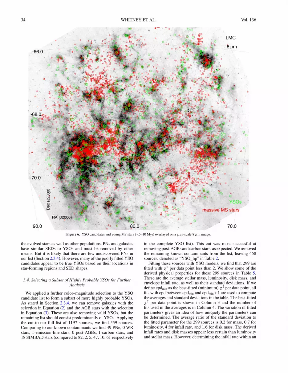
Figure 5 shows the YSO candidate list overlayed on theIRAC 8 µm image. The YSOs appear to be spatially correlatedwith the brighter 8 µm diffuse emission. Figure 6 shows thesame as Figure 5 but zoomed in, and with massive MS starsoverlayed in red. These stars have a mass greater than 10 M�and ages less than 5–10 Myr. They were selected from theMCPS Catalog (Zaritsky et al. 2004) using the following criteria:V < 16 and B − V < 0.5 and V < 15.2 + 3.2(B − V ),where Q is the reddening-free parameter defined by Q =(U − B) − 0.72(B − V ). The massive MS stars tend to clusterinside the bubbles and the YSOs lie in the shells formed bythe bubbles. This is consistent with both triggering in thecompressed shells formed by the previous generation of massivestars (Oey & Massey 1995; Efremov & Elmegreen 1998b), aswell as the stochastic self-propagating star-formation scenariodue to differential rotation of the galaxy (Feitzinger et al. 1981).Figure 7 shows a three-color IRAC+MIPS zoom of the N11region, with the YSOs overlayed. The lack of YSOs in the


Figure 4. Color–color and color–magnitude plots of our candidate YSO list in black, with known sources overplotted in colors indicated by the key and described inSection 3.1. The purple lines in the top two panels show more stringent cuts we could made on the final list to remove galaxies (top left panel) and AGB stars (topright).

central region suggests that our list is incomplete due to brightbackgrounds. Also, extended sources at IRAC bands are missingfrom our Point Source Catalog (for example, the string of foursources on the far-eastern side of the image).

Figure 8 shows the YSOs overlayed on a two-color image ofH i gas (Staveley-Smith et al. 2003) in green and CO gas (Fukuiet al. 1999) in red. The YSOs appear to be associated withboth the neutral and molecular gas, with a preference for themolecular gas (yellow and red). This will be quantified shortlywith correlation plots. The southeast ridge and arc at lowerleft are prominent in the CO (in red and yellow). This is theleading edge of the LMC in its motion through the halo of theMilky Way. de Boer et al. (1998) proposed that star formation istriggered in this compressed region due to the bowshock of theLMC. As the galaxy rotates clockwise, material moves away (tothe north), and we should find a progression in the ages towardthe north. To the north lies in succession N159, 30 Doradus, andin the far north, the large LMC 4 shell, each successively older,so the picture qualitatively fits. We do see active star formationin the southeast ridge, as indicated by the number of YSOs inFigures 5 and 8. In fact, Indebetouw (2008) find an SFR in thisregion of 0.14 M� yr−1 kpc−2, which is a few times higher thanthe global rate per area estimated in this paper (Section 3.5).

Figures 5 and 8 show that the YSO candidates are spatiallycorrelated with the gas in the galaxy. This can be quantified in

several ways. First, we can calculate the correlation coefficientsbetween the spatial density of YSOs and the CO and H i columndensities. The spatial density of candidates can be calculatedrobustly at 10 arcmin resolution (interpretation at finer spatialresolution is difficult with only about 40 sources per squaredegree), and the CO and H i maps were smoothed to the sameresolution. This gives correlation coefficients of 0.82 ± 0.03and 0.73 ± 0.05, for the CO and H i maps, respectively. Theuncertainty quoted is the spread in the result using differentsmoothing kernels and using either a fixed grid or density-scaledgrid method to construct the source density map.

Another measure of gas–YSO correlation is the distribu-tion of gas column density at the location of the YSOs com-pared to the distribution for the general Point Source Catalog.Figures 9–11 shows these distributions for H i, CO, 24 µm, and8 µm diffuse emissions. Since the YSO list was initially culledif the diffuse 24 µm emission was greater than 0.08 MJy sr−1,we applied the same culling to the general catalog in these plots.Then if the YSOs show more correlation, it is due to a real spa-tial association. These figures show that YSO candidates arestatistically associated with greater amounts of gas than genericpoint sources in the LMC. The peak of the column densitydistribution associated with YSOs is ∼2×1021cm−2 of atomichydrogen (Figure 9, left). This is consistent with the thresh-old for the formation of molecular material (approximately


Table 3Previously Known YSOs

Source R.A. (J2000) Decl. (J2000) IRAC designation Separation Ref.(h m s) (◦ ′ ′′) IRAC/MIPS

(arcsec)

30Dor-NIC15a. . . 05 38 48.30 −69 04 10.3 · · · · · · 130Dor-NIC15b. . . 05 38 48.45 −69 04 12.0 · · · · · · 130Dor-NIC16a. . . 05 38 41.62 −69 03 54.7 SSTISAGE1C J053841.36-690354.2 1.5 1N159-P1. . . 05 39 59.36 −69 45 26.3 SSTISAGE1C J053959.30-694526.2 0.3 2N159-P2a. . . 05 39 41.88 −69 46 12.2 SSTISAGE1C J053941.85-694611.9 0.3 2N159-No.9. . . 05 39 37.12 −69 45 37.0 SSTISAGE1C J053937.01-694536.7 0.6 2N159-No.134. . . 05 40 19.12 −69 44 45.6 SSTISAGE1C J054018.97-694445.5 0.8 2N159A6-151b. . . 05 39 36.17 −69 46 04.3 SSTISAGE1C J053935.97-694604.0 1.1/1.0 3N160A. . . 05 39 43.66 −69 38 30.2 SSTISAGE1C J053943.82-693833.8 3.8 4IRAS05328-6827. . . 05 32 38.59 −68 25 22.2 SSTISAGE1C J053238.58-682522.3 0.2/0.6 5N157B IRS1. . . 05 37 50.3 −69 11 07 SSTISAGE1C J053750.28-691107.1 0.1 6N105A IRS1. . . 05 09 50.6 −68 53 05 SSTISAGE1C J050950.53-685305.4 0.6 6N51D YSO-1. . . 05 26 01.30 −67 30 11.8 SSTISAGE1C J052601.22-673011.8 0.5/0.6 7N51D YSO-2. . . 05 26 04.01 −67 29 57.0 · · · · · · 7N51D YSO-3. . . 05 26 19.91 −67 30 33.3 SSTISAGE1C J052619.79-673033.3 0.7/0.9 7LTS J054427-692659c. . . 05 44 27.47 −69 26 59.2 · · · · · · 8

ELHC7d. . . 05 16 39.5 −69 20 49 SSTISAGE1C J051639.18-692048.1 1.9 9ELHC13e. . . 05 18 54.91 −69 36 35.8 SSTISAGE1C J051854.69-693635.5 1.1/1.4 9ELHC19 e. . . 05 17 11.80 −69 25 54.0 SSTISAGE1C J051711.59-692555.3 1.8 9

Notes.a P2 was resolved into two components by Testor et al. ( 2006, resolution 0“.2): N159A7-121 (α = 05h39m41.96s andδ = −69◦46′11.99′′, J2000) and N159A7-123 (α = 05h39m41.90s and δ = −69◦46′11.52′′, J2000), both classifiedas Class I YSOs.b The compact source N159A6 discovered by Testor et al. (2006) consists of two objects contained within a diameterof 0.5 pc: an YSO N159A6-151 and a CHII/HII region containing about five stars. At the IRAC resolution of 2′′(0.48 pc at 50 kpc), N159A6 will be either unresolved or only slightly resolved.c LTS (“LMC T Tauri Star”) J054427-692659 is the first spectroscopically confirmed discovery of T Tauri star inthe LMC.d ELHC stands for EROS LMC HAe/Be Candidates Lamers et al. (1999). ELHC7 is a confirmed HAe/Be UXOrionisstar.e de Wit et al. (2005) suggested that the type of variability of these sources could be interpreted as caused by variabledust obscuration; thus it is possible that they are pre-MS objects. However, these sources lack thermal dust emissionin the near IR. The circumstellar dust emission could be revealed in the mid- or far IR; thus the observations at thesewavelengths are crucial to confirm that these objects are in a pre-MS stage.References.(1) Brandner et al. (2001); (2) Jones et al. (2005); (3) Testor et al. (2006); (4) Epchtein et al. (1984); (5) van Loonet al. (2005); (6) Oliveira et al. (2006); (7) Chu et al. (2005); (8) Wichmann et al. (2001); (9) de Wit et al. (2005),and references therein.

1021 cm−2, somewhat higher with the porous geometry, lowermetallicity, and lower dust-to-gas ratio). On the other hand, thisvalue may only be coincidental, since the column density as-sociated with generic catalog sources peaks only about a factorof 2 lower, because the typical value of the H i column den-sity in the galaxy is 1021 cm−2. Additionally, in many placesalong the line of sight there are (at least) two kinematically andlikely physically distinct gas components (Luks & Rohlfs 1992;Mizuno et al. 2001) so the relevant column for self-shieldingmay be less than half of the total along the line of sight.

The right panel of Figure 9 shows the relative distributionsof YSOs and point sources as a function of peak H i intensityrather than the total column. One might expect the peak H i tobetter reflect the densest individual clouds along the sightline,and correlate better with star formation. Indeed, the distributionsare rather more separated than for column density.

The relative distributions as a function of CO column density(Figure 10) are similar to those for H i, with a shift at afew 1020 cm−2, when using a Galactic value of the X-factor(for converting CO column density to H2), 3×1020 cm−2

(K km s−1)−1. If we adopt a higher value of the X-factor, as

suggested by various studies including the NANTEN survey(Fukui et al. 1999), the characteristic value is approximately1021 cm−2. As expected, there is a stronger association withdense CO gas than H i gas.

Figure 11 shows the spatial association of YSOs with 24 µmand 8 µm surface brightness. At first glance, it appears thatthe YSOs are more strongly associated with higher levels of8 µm flux than 24 µm flux. However, the YSO distributionsthemselves, shown as hatched regions, are fairly similar in thetwo panels. It is the SAGE Catalog, in gray, that is different,associated with low values of 8 µm sky and with a range of24 µm sky values. The SAGE Catalog consists mostly of starsdetected in the 3.6 and 4.5 µm bands. As Figure 6 shows, themassive stars are located preferentially inside the 8 µm shellsand H ii regions. A similar effect is seen in the SMC where theregions surrounding ionizing sources are mostly devoid of 8 µmemission (Bolatto et al. 2007). The 24 µm diffuse emission isbright in the shells but also bright inside the H ii regions wheremassive stars are found, as seen in Figure 4 of Meixner et al.(2006) and in Figure 7 of this paper. Thus, the massive starsare spatially anti-correlated with 8 µm emission and associated


Table 4Previously Known YSOs: Magnitudesa

Source 2MASS IRAC MIPS Ref.

J H Ks [3.6] [4.5] [5.8] [8.0] [24]

30Dor-NIC15a. . . 19.01(0.08)b 18.24(0.13)b 17.57(0.16)b 130Dor-NIC15b. . . 17.06(0.07)b 15.25(0.11)b 13.49(0.12)b 9.24(0.04)c 8.53(0.04)c 6.76(0.04)c 4.97(0.04)c <0.61(0.11)d 130Dor-NIC16a. . . 15.74(0.08) 13.31(0.02) 11.51(0.02) 9.12(0.06) 8.44(0.09) 7.66(0.03) 6.86(0.03) . . . 1N159-P1. . . 16.46(0.17) 13.97(0.08) 11.84(0.03) 9.38(0.07) 8.53(0.07) 7.81(0.04) 6.77(0.05) . . . 2N159-P2. . . 15.29(0.19) 14.04(0.15) 12.16(0.05) 9.37(0.09) 8.22(0.07) 7.13(0.04) 6.00(0.08) 0.74(0.01)c 2N159-No.9. . . 15.55b 14.25b 14.23(0.12) 10.92(0.09) 9.57(0.07) 8.16(0.06) 6.96(0.10) 0.93(0.01)c 2N159-No.134. . . . . . . . . . . . 14.28(0.11) 12.89(0.14) 11.58(0.10) . . . . . . 2N159A6-151. . . 17.91b . . . 14.47b 11.24(0.12) . . . 9.02(0.11) . . . 2.00(0.02) 3N160A. . . 14.17(0.21) 14.04(0.38) 12.90(0.15) 9.62(0.09) 7.48(0.05) 5.80(0.03) 4.63(0.04) . . . 4IRAS05328-6827. . . 16.65(0.20) 14.24(0.06) 11.98(0.03) 8.89(0.05) 7.79(0.05) 6.87(0.02) 5.92(0.02) 2.23(0.01) 5N157B IRS1. . . 15.93(0.12)b 14.22(0.07) 11.45(0.03) 7.87(0.04) 6.78(0.03) 5.86(0.03) 4.89(0.02) 0.69(0.01)c 6N105A IRS1. . . >15.3b >14.7b 13.77(0.10) 10.14(0.04) 8.61(0.04) 7.18(0.02) 5.24(0.02) . . . 6N51D YSO-1. . . . . . . . . . . . 12.06(1.21)b 10.66(0.08) 9.38(0.06) 8.08(0.06) 3.15(0.01) 7N51D YSO-2. . . . . . . . . . . . 13.16(1.32)b 12.74(1.27)b 10.98(1.10)b 9.36(0.94)b 5.55(0.56)b 7N51D YSO-3. . . . . . . . . 14.95(0.13) 12.96(0.1) 12.29(0.08) 10.89(0.05) 9.48(0.07) 6.40(0.01) 7LTS J054427-692659. . . 20.73(0.09)b 19.45(0.04)b 18.57(0.06)b . . . . . . . . . . . . . . . 8ELHC7. . . 17.60b 16.99b 15.96b 14.02(0.04) 13.60(0.06) 13.34(0.08) 13.06(0.09) . . . 9ELHC13. . . . . . . . . . . . . . . 14.51(0.12) . . . . . . 8.10(0.05) 9ELHC19. . . 16.35b 16.23b 16.10b 16.05(0.11) 16.09(0.14) . . . . . . . . . 9

Notes.a Magnitudes from the SAGE Catalog are given where available.b Data from literature (see references below).c Magnitudes measured in this work using aperture photometry.d Source saturated at 24 µm.References.(1) Brandner et al. (2001); (2) Jones et al. (2005); (3) Testor et al. (2006); (4) Epchtein et al. (1984); (5) van Loon et al. (2005); (6) Oliveira et al. (2006); (7) Chuet al. (2005); (8) Wichmann et al. (2001); (9) de Wit et al. (2005), and references therein.

with 24 µm emission in H ii regions, whereas the YSOs areassociated with high 8 µm emission. This is another way ofshowing the visual result from Figure 6 that star formation takesplace in the shells created by the previous generation of high-mass star formation (the massive stars inside the shells).

Figure 12 shows the two-point correlation function of YSOcandidates compared to generic point sources. The generic pointsources (dot-dashed) are not clustered, but the YSOs (dashed)are highly clustered, as expected if star formation takes place infilamentary gas clouds. The YSOs in H i clouds (solid sourcesassociated with >30 K km s−1) are even more clustered. Thesedata do not show any particular characteristic physical scale(as would be evident in a break in the power-law slope of thecorrelation function). If star formation is dominated by self-propagation in overlapping supershells (Oey & Massey 1995;Efremov & Elmegreen 1998a), it should be fairly scale-free inthe range of physical scales we are able to probe, but it is possiblethat the tail of elevated correlation at size scales of ∼0.1◦ �450 pc is associated with supershells.

Figure 12 also shows the nearest-neighbor distribution of ourYSO candidates. The nearest-neighbor distribution can reflectsize scales in the molecular cloud at the time of star formation—for example in the Galaxy, a signature of the cloud’s Jeans lengthhas been seen in the YSO distribution of NGC2264 (Teixeiraet al. 2006) and possibly in M16 (Indebetouw et al. 2007). Inthe LMC we see an excess in the nearest-neighbor distributionof YSOs compared to generic point sources at the smallestsize scales to which our analysis is sensitive (∼10′′ � 3 pc).Given that we are limited by the spatial resolution at 24 µm,we cannot interpret this as a physical scale, but this providesfurther evidence that YSO candidates are highly clustered in thesmallest scales accessible to Spitzer.

3.3. Linear Regression SED Fitting to All the Sources

We fitted YSO models to the SEDs of all of the sources inTable 1, using the model grid described in Robitaille et al. (2006)and the fitting method described in Robitaille et al. (2007). Basedon recent experience fitting YSO data (Robitaille et al. 2007;Indebetouw et al. 2007; Simon et al. 2007; Shepherd et al. 2007;Watson et al. 2008) we reset the photometric errors to 10% ineach band. This allows for other errors (systematic, calibration,variability) besides the photon-counting errors usually quoted.We define well-fitted models as those whose χ2 per data pointis less than two, based on by-eye examination of the fits. Inmany cases, the poorly-fitted sources are due to one bad datapoint, mismatch between 2MASS and Spitzer due to variability,multiple sources in the beam, or inadequacies in the models.Thus a poor fit does not necessarily indicate that the source isnot a YSO.

Example SEDs and YSO fits of different categories of objectsare shown in Figure 13, and the rest are available in the onlinejournal (Figures 13.1–13.80). For the list with identified non-YSO sources removed, 570/990 sources were well fitted (that is,have a χ2 per data point less than 2). Thus, 58% of the candidateYSOs were well fitted by YSO models. For the PNs 54/82 (65%)were well fitted by the YSO models. The SEDs and colors ofthe PNs generally resemble those of the YSOs as shown inFigures 3 and 13. For the other categories, 16/117 (14%) evolvedstars were well fitted, SN87a was well fitted, 2/4 galaxies werewell fitted, and 2/2 X-ray sources were well fitted. Note that alower fraction of evolved stars were well fitted than any othercategory. Thus the YSO fitter can be used to identify suspectedevolved stars as poorly fitted with YSO models. A commonreason for the poor fits of the evolved stars are that the YSO


SIMBAD misc.

Dec

(J20

00)

m image8

LMC

µEM/WR starsPAGB/C stars

PNeYSO Candidates

RA (J2000)

70.080.090.0

-72.0

-70.0

-68.0

-66.0

-64.0

Figure 5. YSO candidates overlayed on a gray-scale 8 µm image of the LMC. The sources identified as other populations (Section 2.3.3) are also shown, color codedas in the key.

models do not have the high luminosity but relatively coolphotospheres needed to fit these sources. An example of this isshown in the bottom two panels of Figure 14. At the left is a YSOfit with a stellar temperature of ∼30,000 K and an IR excess froma disk. The bottom right-hand panel shows that a YSO model at adistance of only 1.5 kpc is easily well fitted with a photosphere of∼6600 K. For these sources to be fitted with YSO models, eitherthe pre-MS evolutionary tracks need to be modified to allow forlarger stellar radii for a modest stellar temperature, or clustersof stars with average photospheric temperatures of 5000 Kare required to fit the sources. More likely, they are evolved starswith expanded, luminous, and relatively cool photospheres.

Some examples of poorly-fitted YSOs are given in Figure 14.Based on their location in the N11 star-forming region (sources“3” and “4” in Figure 7) and their SED shapes, these are likelytrue YSOs. The reason the source on the left is not well fitted is

that it probably has PAH emission, which is not accounted forin our models. This gives an excess at 3.6, 5.8, and especially8 µm, compared to 4.5. The source on the right has higherJHKs fluxes than is typical of an embedded YSO. There couldbe several reasons for this: variability of the source between theepochs of the 2MASS and SAGE observations; multiple sourcesin the beam (one optically bright and one IR bright); orincomplete sampling of model parameters in the grid. At adistance of the LMC, it would not be surprising to have morethan one source in the 0.5–1 pc IRAC beam. Also noticeable inthe SEDs in Figure 13.1–13.80 are the noisier 2MASS datarelative to the deeper SAGE data. This contributes severalpoorly-fitted SEDs as well. In addition the 2MASS resolutionis 50% worse than IRAC, contributing to the confusion issue.

From these fits, we conclude that the YSO fitter can be usedas an additional tool to remove contaminants since it does not fit


Dec

(J20

00)

RA (J2000)

mµ8

LMC

massive MS stars

YSOs

70.080.090.0

-70.0

-68.0

-66.0

Figure 6. YSO candidates and young MS stars (<5–10 Myr) overlayed on a gray-scale 8 µm image.

the evolved stars as well as other populations. PNs and galaxieshave similar SEDs to YSOs and must be removed by othermeans. But it is likely that there are few undiscovered PNs inour list (Section 2.3.4). However, many of the poorly fitted YSOcandidates appear to be true YSOs based on their locations instar-forming regions and SED shapes.

3.4. Selecting a Subset of Highly Probable YSOs for FurtherAnalysis

We applied a further color–magnitude selection to the YSOcandidate list to form a subset of more highly probable YSOs.As stated in Section 2.3.4, we can remove galaxies with theselection in Equation (2) and the AGB stars with the selectionin Equation (3). These are also removing valid YSOs, but theremaining list should consist predominantly of YSOs. Applyingthe cut to our full list of 1197 sources, we find 559 sources.Comparing to our known contaminants we find 49 PNe, 0 WRstars, 1-emission-line stars, 0 post-AGBs, 1-carbon stars, and18 SIMBAD stars (compared to 82, 2, 5, 47, 10, 61 respectively

in the complete YSO list). This cut was most successful atremoving post-AGBs and carbon stars, as expected. We removedthe remaining known contaminants from the list, leaving 458sources, denoted as “YSO_hp” in Table 2.

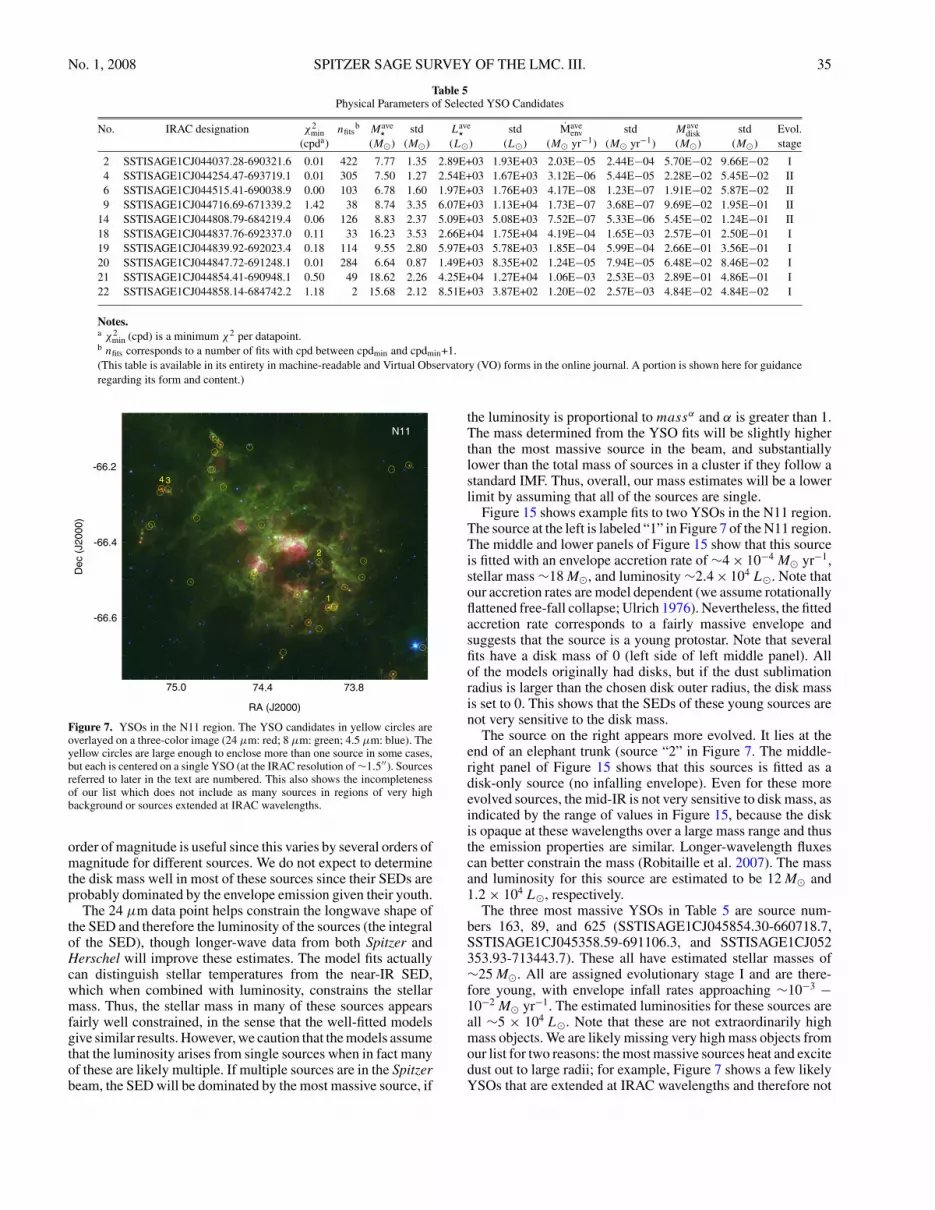
Fitting these sources with YSO models, we find that 299 arefitted with χ2 per data point less than 2. We show some of thederived physical properties for these 299 sources in Table 5.These are the average stellar mass, luminosity, disk mass, andenvelope infall rate, as well as their standard deviations. If wedefine cpdmin as the best-fitted (minimum) χ2 per data point, allfits with cpd between cpdmin and cpdmin + 1 are used to computethe averages and standard deviations in the table. The best-fittedχ2 per data point is shown in Column 3 and the number offits used in the averages is in Column 4. The variation of fittedparameters gives an idea of how uniquely the parameters canbe determined. The average ratio of the standard deviation tothe fitted parameter for the 299 sources is 0.2 for mass, 0.7 forluminosity, 4 for infall rate, and 1.6 for disk mass. The derivedinfall rates and disk masses appear less certain than luminosityand stellar mass. However, determining the infall rate within an


Table 5Physical Parameters of Selected YSO Candidates

No. IRAC designation χ2min nfits

b Mave� std Lave

� std Maveenv std Mave

disk std Evol.(cpda) (M�) (M�) (L�) (L�) (M� yr−1) (M� yr−1) (M�) (M�) stage

2 SSTISAGE1CJ044037.28-690321.6 0.01 422 7.77 1.35 2.89E+03 1.93E+03 2.03E−05 2.44E−04 5.70E−02 9.66E−02 I4 SSTISAGE1CJ044254.47-693719.1 0.01 305 7.50 1.27 2.54E+03 1.67E+03 3.12E−06 5.44E−05 2.28E−02 5.45E−02 II6 SSTISAGE1CJ044515.41-690038.9 0.00 103 6.78 1.60 1.97E+03 1.76E+03 4.17E−08 1.23E−07 1.91E−02 5.87E−02 II9 SSTISAGE1CJ044716.69-671339.2 1.42 38 8.74 3.35 6.07E+03 1.13E+04 1.73E−07 3.68E−07 9.69E−02 1.95E−01 II

14 SSTISAGE1CJ044808.79-684219.4 0.06 126 8.83 2.37 5.09E+03 5.08E+03 7.52E−07 5.33E−06 5.45E−02 1.24E−01 II18 SSTISAGE1CJ044837.76-692337.0 0.11 33 16.23 3.53 2.66E+04 1.75E+04 4.19E−04 1.65E−03 2.57E−01 2.50E−01 I19 SSTISAGE1CJ044839.92-692023.4 0.18 114 9.55 2.80 5.97E+03 5.78E+03 1.85E−04 5.99E−04 2.66E−01 3.56E−01 I20 SSTISAGE1CJ044847.72-691248.1 0.01 284 6.64 0.87 1.49E+03 8.35E+02 1.24E−05 7.94E−05 6.48E−02 8.46E−02 I21 SSTISAGE1CJ044854.41-690948.1 0.50 49 18.62 2.26 4.25E+04 1.27E+04 1.06E−03 2.53E−03 2.89E−01 4.86E−01 I22 SSTISAGE1CJ044858.14-684742.2 1.18 2 15.68 2.12 8.51E+03 3.87E+02 1.20E−02 2.57E−03 4.84E−02 4.84E−02 I

Notes.a χ2

min (cpd) is a minimum χ2 per datapoint.b nfits corresponds to a number of fits with cpd between cpdmin and cpdmin+1.(This table is available in its entirety in machine-readable and Virtual Observatory (VO) forms in the online journal. A portion is shown here for guidanceregarding its form and content.)

N11

Dec

(J20

00)

RA (J2000)

73.874.475.0

-66.6

-66.4

-66.24 3

1

2

Figure 7. YSOs in the N11 region. The YSO candidates in yellow circles areoverlayed on a three-color image (24 µm: red; 8 µm: green; 4.5 µm: blue). Theyellow circles are large enough to enclose more than one source in some cases,but each is centered on a single YSO (at the IRAC resolution of ∼1.5′′). Sourcesreferred to later in the text are numbered. This also shows the incompletenessof our list which does not include as many sources in regions of very highbackground or sources extended at IRAC wavelengths.

order of magnitude is useful since this varies by several orders ofmagnitude for different sources. We do not expect to determinethe disk mass well in most of these sources since their SEDs areprobably dominated by the envelope emission given their youth.

The 24 µm data point helps constrain the longwave shape ofthe SED and therefore the luminosity of the sources (the integralof the SED), though longer-wave data from both Spitzer andHerschel will improve these estimates. The model fits actuallycan distinguish stellar temperatures from the near-IR SED,which when combined with luminosity, constrains the stellarmass. Thus, the stellar mass in many of these sources appearsfairly well constrained, in the sense that the well-fitted modelsgive similar results. However, we caution that the models assumethat the luminosity arises from single sources when in fact manyof these are likely multiple. If multiple sources are in the Spitzerbeam, the SED will be dominated by the most massive source, if

the luminosity is proportional to massα and α is greater than 1.The mass determined from the YSO fits will be slightly higherthan the most massive source in the beam, and substantiallylower than the total mass of sources in a cluster if they follow astandard IMF. Thus, overall, our mass estimates will be a lowerlimit by assuming that all of the sources are single.

Figure 15 shows example fits to two YSOs in the N11 region.The source at the left is labeled “1” in Figure 7 of the N11 region.The middle and lower panels of Figure 15 show that this sourceis fitted with an envelope accretion rate of ∼4 × 10−4 M� yr−1,stellar mass ∼18 M�, and luminosity ∼2.4 × 104 L�. Note thatour accretion rates are model dependent (we assume rotationallyflattened free-fall collapse; Ulrich 1976). Nevertheless, the fittedaccretion rate corresponds to a fairly massive envelope andsuggests that the source is a young protostar. Note that severalfits have a disk mass of 0 (left side of left middle panel). Allof the models originally had disks, but if the dust sublimationradius is larger than the chosen disk outer radius, the disk massis set to 0. This shows that the SEDs of these young sources arenot very sensitive to the disk mass.

The source on the right appears more evolved. It lies at theend of an elephant trunk (source “2” in Figure 7. The middle-right panel of Figure 15 shows that this sources is fitted as adisk-only source (no infalling envelope). Even for these moreevolved sources, the mid-IR is not very sensitive to disk mass, asindicated by the range of values in Figure 15, because the diskis opaque at these wavelengths over a large mass range and thusthe emission properties are similar. Longer-wavelength fluxescan better constrain the mass (Robitaille et al. 2007). The massand luminosity for this source are estimated to be 12 M� and1.2 × 104 L�, respectively.

The three most massive YSOs in Table 5 are source num-bers 163, 89, and 625 (SSTISAGE1CJ045854.30-660718.7,SSTISAGE1CJ045358.59-691106.3, and SSTISAGE1CJ052353.93-713443.7). These all have estimated stellar masses of∼25 M�. All are assigned evolutionary stage I and are there-fore young, with envelope infall rates approaching ∼10−3 −10−2 M� yr−1. The estimated luminosities for these sources areall ∼5 × 104 L�. Note that these are not extraordinarily highmass objects. We are likely missing very high mass objects fromour list for two reasons: the most massive sources heat and excitedust out to large radii; for example, Figure 7 shows a few likelyYSOs that are extended at IRAC wavelengths and therefore not


YSOsHICO

Dec

(J20

00)

RA (J2000)

70.075.080.085.090.0

-71.0

-69.0

-67.0

-65.0

Figure 8. YSOs (magneta circles) overlayed on a two-color image of H i gas in green, and CO gas in red.

Figure 9. Left: distribution of YSO candidates (hashed) and of the entire SAGE Catalog (gray) as a function of H i column density (in units of 1020 cm−2). The YSOcandidates are associated with higher columns of ISM than those of the SAGE Catalog. Right: distribution of YSO candidates and of the entire SAGE Catalog as afunction of H i peak intensity.


Figure 10. Distribution of YSO candidates (hashed) and of the entire SAGECatalog (gray) as a function of CO column density (units of 1020 cm−2).

in our Point Source Catalogs. Second, these massive YSOs mayoverlap in color–magnitude space with the most luminous AGBstars as shown in Figure 3. This region of color–magnitude spacewas avoided in our high-probability YSO selection.

The total mass of well-fitted YSOs is estimated to be2900 M�, and the total luminosity is 2 × 106L�. These werecalculated by summing the averages of all the well-fittedmodels. Figure 16 shows histograms of the estimated massesand luminosities of the well-fitted YSOs. Note that some of thenumber values are less than 1, because it is a histogram of allthe well-fitted distributions (normalized to the number of fits),instead of the average value for each source. The rounded shapesof the histograms show incompleteness at both ends of themass spectrum. As mentioned previously, we are missing somehigh-mass sources that are extended at the IRAC wavelengths.Another reason for the fall-off at the high-mass end couldbe because of the faster evolution expected for the high-massprotostars and thus shorter YSO lifetimes. Our mass function isa YSO mass histogram and not a stellar IMF. And of course weare missing low-luminosity sources due to our selection criteriaavoiding the lower-luminosity background galaxies. Our massfunction may be complete over the range of ∼6–10 M�. We notethat the mass estimates assume that a single source produces themeasured SED. As noted previously, our mass estimates are a

lower limit by assuming that all of the sources are single. All ofthis points to a likely lower limit in our estimate of YSO masses.

Using the derived parameters to estimate evolutionary stage,Table 5 has 145 Stage I (young embedded) sources, 147Stage II (optically thick disk) sources, and seven Stage III(optically thin disk) sources. If we had an unbiased list ofYSOs, we could estimate evolutionary timescales from the ratiosof the numbers at different stages. In the Taurus molecularcloud, for example, there are roughly ten times more StageII sources than Stage I sources, and therefore the embeddedinfalling envelope stage is thought to have a lifetime roughly1/10th as long as the star+disk stage (105 years versus 106

years, respectively; Lada 1999). If we assume evolutionarytimescales are similar to Taurus, it is clear that our YSOlist is biased toward younger sources since the number ofStage I sources is similar to that of the Stage II sources. Thisis not surprising since we have only selected sources with red[8.0]−[24] colors for this high-probability YSO list.

3.5. The Current Star-Formation Rate and Efficiency of theLMC

We can calculate the current SFR by estimating the total massof YSOs and dividing by a formation timescale. To estimatethe total mass, we attach a Kroupa (2001) IMF to our massfunction over the narrow range that our source list may becomplete (Figure 16). Rather than fitting an uncertain slope,we adopt the Kroupa average slopes of −1.3 for M� > 0.5,and −0.3 for M� < 0.5. Our integration limits went from 0.08to 50 solar masses. Clearly the choice of both the slope andlower integration limit has a large effect on the total estimatedmass. Integrating the Kroupa IMF gives a total mass of YSOsof 11300 M�. We include the masses derived only from the299 well-fitted high-probability YSOs shown in Table 5. Sincemost of the YSOs in Table 5 are young and relatively massive,we assume a formation timescale of ≈2 × 105 yr. This givesan SFR of 0.06M� yr−1. This is likely uncertain by an orderof magnitude given our uncertain estimates of both mass andlifetime.

We can compare this estimate to those calculated fromintegrating global fluxes. The Kennicutt (1998) relations forultraviolet and far-IR fluxes give 0.08M� yr−1 and 0.17M� yr−1

respectively, using the rocket ultraviolet image of Smith et al.(1987) and the SAGE MIPS data (at 24, 70, and 160 µm) for thethermal IR flux (see Dale & Helou 2002). The new calibrations

Figure 11. Distribution of YSO candidates (hashed) and of the entire SAGE Catalog (gray) as a function of 24 µm intensity (left) and 8 µm intensity (right) (units ofMJy sr−1). The main difference between these panels is in the catalog distribution rather than the YSOs. The catalog sources peak in regions of low 8 µm emission,in agreement with Figure 6 which shows massive stars inside the 8 µm bubbles.


Figure 12. Two measures of clustering of the YSO candidates. The left panel shows the two-point correlation functions of YSOs (dashed and solid lines) and genericSAGE Point Sources (dot-dashed). A break in the correlation function can indicate a preferred scale for star formation, such as a Jeans mass, but the roughly power-lawform seen here merely indicates strong hierarchical clustering on all scales. The right panel shows the nearest-neighbor distribution of the relevant populations. Anexcess at small scales in this distribution can indicate a fragmentation or other preferred clustering scale. LMC YSOs are tightly clustered down to the smallest scalesthat we can measure (∼10′′). In the key, “contaminants” refer to the sources identified as non-YSOs.

from Calzetti et al. (2007) give an SFR of 0.05M� yr−1 usingthe SAGE MIPS24 image, and 0.14 M� yr−1 using the SouthernH-Alpha Sky Survey Atlas (SHASSA) images (Gaustad et al.2001). The combined rates from H-alpha and MIPS24 (Calzettiet al. 2007) give 0.19 M� yr−1 for stars with age <10 Myr. Theultraviolet and thermal IR combined rates are 0.25 M� yr−1 forstars < 100 Myr old. These estimates agree with that madeby Kennicutt et al. (1995) based on the H-α luminosity if weuse the newer conversion factors (Kennicutt 1998) and make a0.3 mag correction for extinction.

Gorjian et al. (2004) estimated the SFR of the star-formingregion Henize 206 in the LMC, also using the Kennicutt (1998)relations, and calculated a value of 1×10−3 M� yr−1 for an areaof 0.021 deg2, or 8 × 10−3 M�yr−1 kpc−2 (assuming a distanceto the LMC of 50 kpc). Indebetouw (2008) estimated the SFRof the southeast (SE) ridge (discussed in Section 3.2) using theSchmitt–Kennicutt law (Kennicutt 1998) and found a value of0.14 M� yr−1 kpc−2. A rough estimate of the total star-formingarea of the LMC can be made from the extent of the detectableH i and 70 µm emission. From this we estimate the area tobe 34 kpc2 or 44 deg2. Scaling the global value calculatedabove, we obtain ≈5 × 10−3M�yr−1 kpc−2. Based on thesecalculations, the SE ridge does appear to be more active thanaverage, in agreement with models that suggest triggered starformation in this region (de Boer et al. 1998). Simon et al. (2007)calculated the SFR for the N66 region in the SMC, also usingYSO SED fitting, and found a rate of 0.066 M� yr−1 kpc−2

consistent with its being the most active star-formation regionin the SMC.

As noted in Section 1, optical CMD modeling has determinedhistorical relative rates of star formation in the LMC (e.g.,Gallagher et al. 1996; Olsen 1999; Smecker-Hane et al. 2002).The LMC is thought to be in an active period of star and clusterformation currently (Da Costa 1991; Hodge 1988), with anincrease in the SFR from 3–4 Gyr ago by a factor of about3 (Geha et al. 1998; Holtzman et al. 1997). This is consistent

with the new results (Kallivayalil et al. 2006b, 2006a; Beslaet al. 2007) suggesting that the LMC is in its first passage withthe Milky Way, having entered the virial radius of the darkmatter halo 1–3 Gyr ago. The SFR estimated by the YSOsand integrated fluxes set an absolute scale to the star-formationhistory.

The star-formation efficiency (SFE) can be estimated bydividing the total mass of YSOs by the mass of molecular gas(∼4×107 M�; Fukui et al. 1999), giving ∼3×10−4, much lowerthan the estimate of 1% (Fukui et al. 1999). Their estimate wasbased on 45 young populous clusters associated with molecularclouds (Bica et al. 1996), assuming a mass of 104M� for each,and dividing by the same molecular gas mass (Fukui et al. 1999).The likely reason for the discrepancy is due to the very differentlifetimes of YSOs and young clusters. To accurately calculatethe SFE, we need to know the molecular cloud lifetimes andthe total number of stars produced in that time. The YSO-basedcalculation is a lower estimate since the time over which theYSOs have strong IR excesses, and are thus selected by themethods in this paper, is likely much shorter than the molecularcloud lifetimes. The cluster estimate is probably more accurate,since the clusters are still associated with the clouds and thusplace lower limits on the age of the clouds.

4. SUMMARY

Our new YSO candidate list increases the number of sus-pected YSOs in the LMC from a handful to over a thousand.The list was selected to contain as many YSOs as possible inregions of color–magnitude space relatively free of other popu-lations, but the resulting list likely includes some evolved starsand galaxies. We estimate a conservative upper limit of 55%contamination by these populations. Follow-up spectroscopicobservations will guide us further in separating these popula-tions. Our YSO list will expand as we include extended IRACsources and long-wave MIPS sources, use future SAGE Catalogs


Figure 13. SEDs of sources of different categories. top left: YSO; top right: QSO; middle left: carbon star; middle right: AGB; bottom left: PN; bottom right: WRstar. The dashed line in each plot is the central stellar atmosphere extincted by the fitted foreground extinction (shown in the plot).(An extended figure set is available in the online journal)

that go deeper, employ statistical methods for source classifica-tion (Harvey et al. 2007; Marengo et al. 2006), and improve ourhigh-mass YSO radiation transfer models. However, the currentlist should be of immediate use for follow-up studies. In ad-dition, users can select the 458 “YSO_hp” sources in Table 2which have a higher probability of being YSOs.

We compared our candidate YSO list to gas tracers (H iand CO) and found it substantially more correlated than theSAGE Catalog. As expected, the correlation is strongest withmolecular gas as traced by CO. The YSOs are correlated with8 µm and 24 µm emission in a similar fashion, but the SAGECatalog sources are correlated significantly more with 24 µmemission than 8 µm (Figure 11). This agrees with the picturealso indicated by Figure 6, in which the massive MS stars arefound in the H ii regions inside the shells in which the YSOs aremore predominantly found. The 24 µm emission is also found in

the H ii regions but the 8 µm emission is mostly in the shells. TheMS stars with ages <10 Myr likely produced the shells in whichthe YSOs are currently forming, in agreement with previouswork suggesting self-propagating star formation (Feitzingeret al. 1981; Oey & Massey 1995; Efremov & Elmegreen 1998a).

The YSOs are more clustered than generic catalog sources,as shown in Figure 12. The roughly power-law shape of thetwo-point correlation function indicates similar clustering onall scales (hierarchical), though it is possible that the tail ofelevated correlation on size scales of ∼450 pc is associated withsupershells. The nearest-neighbor distribution shows that YSOsare more clustered than catalog sources down to the smallestscales we can measure, ∼3 pc.

We calculated physical parameters of 299 high-probabilityYSOs whose SEDs were well fitted by a large grid of radi-ation transfer models. These include estimates of stellar mass,


Figure 14. Top: examples of two sources not well fitted by YSO models. Both are likely to be YSOs, but the one at the left probably has PAH emission not accountedfor in our models. The one at the right may include more than one source contributing to the excess near-IR emission not normally associated with an embeddedprotostar. Bottom: at the left is a source poorly fitted by our YSO models fitted with a distance of 50 kpc. At the right is the same source fitted well with a distance ofonly 1.5 kpc. The stellar photospheres are shown as dashed lines, extincted by the fitted foreground value. The stellar temperature for the fit at right is about 6500 K,and the IR excess is modest. This is likely an evolved star, as its SED is similar to one shown in Figure 13 (middle-left panel). The evolved-star models can be fittedwith LMC distances (A. Ginsburg et al. 2008, in preparation).

envelope infall rate, disk mass, and luminosity (Table 5). The es-timated summed mass and luminosity of the YSOs is ∼2900 M�and ∼2 × 106 L�, respectively. Attaching a standard (Kroupa2001) IMF to the mass histogram over the mass range thoughtto be complete (6–10 M�) and integrating gives a total massof YSOs in the LMC of 11300 M�. About half of the sourcesare classified as Stage I, or young sources, still surrounded byinfalling envelopes. This is not surprising because our color–magnitude selection criteria was biased toward redder, and there-fore younger sources.

The SFR of the LMC was calculated by dividing the totalestimated mass of the subset of YSOs (the well-fitted high-probability YSOs) by their estimated ages, giving ∼0.06 M�yr−1 but the uncertainty of this estimate is likely an order ofmagnitude, due to our incomplete source list, uncertain IMF,and uncertain age estimate for the YSOs. In the future, as ourYSO Catalog becomes more complete, the SFR estimates willbecome more accurate. The estimate based on YSO counting islower than most of the estimates calculated from the integratedultraviolet, H-α, and IR fluxes from the LMC, which give∼0.05 − 0.25 M� yr−1. Compared to the Milky Way Galaxy,which has a SFR of ∼5 M� yr−1 (Smith et al. 1978; Diehlet al. 2006) and a total mass ∼50 times greater than the LMC(van der Marel et al. 2002; Besla et al. 2007), the LMC SFR iscomparable or slightly larger than the Galactic rate. Compared tothe SMC, which has an estimated SFR of 0.05 M� yr−1 (Wilkeet al. 2004) and a mass of 5–10 times smaller than the LMC(Besla et al. 2007), the SMC appears to be more active than theLMC at the present time.

To accurately estimate the SFE, we would count all the starsformed during the lifetime of the molecular cloud. Our SFEestimate of 3 × 10−4, based on the ratio of YSO masses tomolecular cloud mass, is a lower limit since the age of the YSOsis likely much younger than the age of the molecular clouds; i.e.,those YSOs that have evolved into MS stars during the lifetimeof the cloud are not being counted. Fukui et al. (1999)’s estimateof 0.01 could be an upper limit if the ages of the associated youngclusters is larger than the molecular cloud lifetime, though it iscertainly more accurate than the YSO estimate. A better estimateof cloud lifetimes in conjunction with star-formation historymodels would improve the SFE estimate. Future work based onthe SAGE data (T. Onishi et al. 2008, in preparation) will betterdetermine cloud lifetimes by determining the number of cloudswith and without star-formation activity.

We thank the anonymous referee whose comments helpedimprove this paper. We thank Eva Villaver for providing helpfulinformation about PNe. This work was supported by NASAgrants to the Spitzer SAGE Legacy project (1275598, 1275588,1282646, 1275421, 397380, 1275471, and 1282688), the SpitzerTheoretical Research Program (1290701; B. W., T. R.), theSpitzer Fellowship Program (R. I.), the NASA Theory Program(NNG05GH35G; B.W.), NASA grant NAG5-12595 (M. M.,U. V.). This research is based on observations made with theSpitzer Space Telescope, which is operated by the Jet PropulsionLaboratory, California Institute of Technology under a contractwith NASA; has made use of data products from the 2MASS,


Figure 15. Example YSO fitter results on two sources. These are sources 1 and 2 in Figure 7. Top: the gray lines show all the models with χ2 per data point betweenthe minimum value, cpdmin, and cpdmin + 1. The dashed line shows the input stellar atmosphere file extincted by the fitted foreground value. The middle and bottompanels show different model parameters for the same set of model fits as the top panel. The contoured gray scale shows how the parameters of the entire model gridare distributed. The source at left is fitted with a substantial envelope and the source at right is fitted with disk-only models and is therefore likely more evolved.

Figure 16. Histograms of stellar mass and luminosity for the well-fitted high-probability YSO candidates (Table 5). The dashed line in the left panel is the (Kroupa2001) IMF (see Section 3.5).


which is a joint project of the University of Massachusettsand the IR Processing and Analysis Center/California Instituteof Technology, funded by NASA and the National ScienceFoundation; and has used the SIMBAD database, operated atCDS, Strasbourg, France.

REFERENCES

Besla, G., Kallivayalil, N., Hernquist, L., Robertson, B., Cox, T. J., van derMarel, R. P., & Alcock, C. 2007, ApJ, 668, 949

Bica, E., Claria, J. J., Dottori, H., Santos, J. F. C. Jr., & Piatti, A. E. 1996, ApJS,102, 57

Blum, R. D., et al. 2006, AJ, 132, 2034Bohannan, B., & Epps, H. W. 1974, A&AS, 18, 47Bolatto, A. D., et al. 2007, ApJ, 655, 212Brandner, W., Grebel, E. K., Barba, R. H., Walborn, N. R., & Moneti, A.

2001, AJ, 122, 858Breysacher, J., Azzopardi, M., & Testor, G. 1999, A&AS, 137, 117Brott, I., & Hauschildt, P. H. 2005, in ESA SP-576, The Three-Dimensional

Universe with Gaia, ed. C. Turon, K. S. O Flaherty, & M. A. C. Perryman,(Noordwijk: ESA), 565

Buchanan, C. L., Kastner, J. H., Forrest, W. J., Hrivnak, B. J., Sahai, R., Egan,M., Frank, A., & Barnbaum, C. 2006, AJ, 132, 1890

Calzetti, D., et al. 2005, ApJ, 633, 871Calzetti, D., et al. 2007, ApJ, 666, 870Chu, Y.-H., et al. 2005, ApJ, 634, L189Cioni, M.-R. L., Girardi, L., Marigo, P., & Habing, H. J. 2006, A&A, 448, 77Cohen, M., et al. 2007, MNRAS, 374, 979Da Costa, G. S. 1991, in IAU Symp. 148, The Magellanic Clouds, ed. R. Haynes,

& D. Milne, (Dordrecht: Kluwer), 183Dale, D. A., & Helou, G. 2002, ApJ, 576, 159de Boer, K. S., Braun, J. M., Vallenari, A., & Mebold, U. 1998, A&A, 329, L49de Wit, W. J., Beaulieu, J. P., & Lamers, H. J. G. L. M. 2002, A&A, 395, 829de Wit, W. J., Beaulieu, J. P., Lamers, H. J. G. L. M., Coutures, C., & Meeus,

G. 2005, A&A, 432, 619Diehl, R., et al. 2006, Nature, 439, 45Diolaiti, E., Bendinelli, O., Bonaccini, D., Close, L., Currie, D., & Parmeggiani,

G. 2000, A&AS, 147, 335Draine, B. T. 2003, ARA&A, 41, 241Efremov, Y. N., & Elmegreen, B. G. 1998a, MNRAS, 299, 588Efremov, Y. N., & Elmegreen, B. G. 1998b, MNRAS, 299, 643Egan, M. P., Van Dyk, S. D., & Price, S. D. 2001, AJ, 122, 1844Ellingsen, S. P., Whiteoak, J. B., Norris, R. P., Caswell, J. L., & Vaile, R. A.

1994, MNRAS, 269, 1019Epchtein, N., Braz, M. A., & Sevre, F. 1984, A&A, 140, 67Fazio, G. G., et al. 2004, ApJS, 154, 10Feitzinger, V., Glassgold, A. E., Gerola, H., & Seiden, P. E. 1981, A&A, 98, 371Fukui, Y., et al. 1999, PASJ, 51, 745Gallagher, J. S., et al. 1996, ApJ, 466, 732Gatley, I., Becklin, E. E., Hyland, A. R., & Jones, T. J. 1981, MNRAS, 197, 17PGaustad, J. E., McCullough, P. R., Rosing, W., & Van Buren, D. 2001, PASP,

113, 1326Geha, M. C., et al. 1998, AJ, 115, 1045Gibb, E. L., et al. 2000, ApJ, 536, 347Giveon, U., Richter, M. J., Becker, R. H., & White, R. L. 2007, AJ, 133, 639Gordon, K. D., et al. 2005, PASP, 117, 503Gorjian, V., et al. 2004, ApJS, 154, 275Gouliermis, D., Brandner, W., & Henning, T. 2006, ApJ, 636, L133Hartmann, L., Ballesteros-Paredes, J., & Bergin, E. A. 2001, ApJ, 562, 852Harvey, P., Merın, B., Huard, T. L., Rebull, L. M., Chapman, N., Evans, N. J.

II, & Myers, P. C. 2007, ApJ, 663, 1149Hodge, P. 1988, PASP, 100, 1051Hollenbach, D., Johnstone, D., Lizano, S., & Shu, F. 1994, ApJ, 428, 654Holtzman, J. A., et al. 1997, AJ, 113, 656Hora, J. L., et al. 2008, AJ, 135, 726Hyland, A. R., Straw, S., Jones, T. J., & Gatley, I. 1992, MNRAS, 257, 391Indebetouw, R. 2008, ApJ, submittedIndebetouw, R., Johnson, K. E., & Conti, P. 2004, AJ, 128, 2206Indebetouw, R., Robitaille, T. P., Whitney, B. A., Churchwell, E., Babler, B.,

Meade, M., Watson, C., & Wolfire, M. 2007, ApJ, 666, 321Indebetouw, R., et al. 2005, ApJ, 619, 931Israel, F. P., et al. 2003, A&A, 406, 817Jones, T. J., Hyland, A. R., Straw, S., Harvey, P. M., Wilking, B. A., Joy, M.,

Gatley, I., & Thomas, J. A. 1986, MNRAS, 219, 603Jones, T. J., Woodward, C. E., Boyer, M. L., Gehrz, R. D., & Polomski, E.

2005, ApJ, 620, 731

Kallivayalil, N., van der Marel, R. P., & Alcock, C. 2006a, ApJ, 652, 1213Kallivayalil, N., van der Marel, R. P., Alcock, C., Axelrod, T., Cook, K. H.,

Drake, A. J., & Geha, M. 2006b, ApJ, 638, 772Keane, J. V., Tielens, A. G. G. M., Boogert, A. C. A., Schutte, W. A., & Whittet,

D. C. B. 2001, A&A, 376, 254Kennicutt, R. C. Jr. 1998, ARA&A, 36, 189Kennicutt, R. C. Jr., Bresolin, F., Bomans, D. J., Bothun, G. D., & Thompson,

I. B. 1995, AJ, 109, 594Kontizas, E., Dapergolas, A., Morgan, D. H., & Kontizas, M. 2001, A&A,

369, 932Kroupa, P. 2001, MNRAS, 322, 231Kurucz, R. 1993, ATLAS9 Stellar Atmosphere Programs and 2 km s−1 Grid.

Kurucz CD-ROM No. 13 (Cambridge, MA: Smithsonian Astrophysical Obs.)13

Kwok, S. 1993, ARA&A, 31, 63Lada, C. J. 1999, in NATO ASIC Proc. 540, The Origin of Stars and Planetary

Systems, ed. C. J. Lada, & N. D. Kylafis, (Dordrecht: Kluwer), 143Lamers, H. J. G. L. M., Beaulieu, J. P., & de Wit, W. J. 1999, A&A, 341, 827Leisy, P., Dennefeld, M., Alard, C., & Guibert, J. 1997, A&AS, 121, 407Lonsdale, C., et al. 2004, ApJS, 154, 54Luks, T., & Rohlfs, K. 1992, A&A, 263, 41Madau, P., Ferguson, H. C., Dickinson, M. E., Giavalisco, M., Steidel, C. C., &

Fruchter, A. 1996, MNRAS, 283, 1388Marengo, M., Allen, L. E., Ashby, M. L., Patten, B. M., Sanchez, M. C., & IRAC

Shallow Survey Collaboration. 2006, in AAS Meeting Abstracts Vol. 209,#161.07 available at http://www.lpi.usra.edu/meetings/ppv2005/pdf/8566.pdf

Meixner, M., et al. 2006, AJ, 132, 2268Mizuno, N., et al. 2001, PASJ, 53, 971Oey, M. S., & Massey, P. 1995, ApJ, 452, 210Oliveira, J. M., van Loon, J. T., Stanimirovic, S., & Zijlstra, A. A.

2006, MNRAS, 372, 1509Olsen, K. A. G. 1999, AJ, 117, 2244Panagia, N. 2005, in IAU Colloq. 192, Cosmic Explosions, On the 10th

Anniversary of SN1993J, ed. J.-M. Marcaide, & K. W. Weiler, (Berlin:Springer), 585

Panagia, N., Romaniello, M., Scuderi, S., & Kirshner, R. P. 2000, ApJ, 539, 197Pei, Y. C., Fall, S. M., & Hauser, M. G. 1999, ApJ, 522, 604Porras, A., et al. 2007, ApJ, 656, 493Reid, W. A., & Parker, Q. A. 2006, MNRAS, 373, 521Rieke, G. H., et al. 2004, ApJS, 154, 25Robberto, M., Beckwith, S. V. W., & Panagia, N. 2002, ApJ, 578, 897Robitaille, T. P., Whitney, B. A., Indebetouw, R., & Wood, K. 2007, ApJS,

169, 328Robitaille, T. P., Whitney, B. A., Indebetouw, R., Wood, K., & Denzmore, P.

2006, ApJS, 167, 256Romaniello, M., Scuderi, S., Panagia, N., Salerno, R. M., & Blanco, C.

2006, A&A, 446, 955Rubio, M., Roth, M., & Garcia, J. 1992, A&A, 261, L29Scalise, E. Jr., & Braz, M. A. 1982, AJ, 87, 528Schoenberner, D. 1981, A&A, 103, 119Schoenberner, D. 1983, ApJ, 272, 708Shepherd, D. S., et al. 2007, ApJ, 669, 464Simon, J. D., et al. 2007, ApJ, 669, 327Skrutskie, M. F., et al. 2006, AJ, 131, 1163Smecker-Hane, T. A., Cole, A. A., Gallagher, J. S. III, & Stetson, P. B. 2002, ApJ,

566, 239Smith, A. M., Cornett, R. H., & Hill, R. S. 1987, ApJ, 320, 609Smith, L. F., Mezger, P. G., & Biermann, P. 1978, A&A, 66, 65Srinivasan, S., et al. 2008, AJ, submittedStaveley-Smith, L., Kim, S., Calabretta, M. R., Haynes, R. F., & Kesteven, M.

J. 2003, MNRAS, 339, 87Stetson, P. B. 1987, PASP, 99, 191Teixeira, P. S., et al. 2006, ApJ, 636, L45Testor, G., Lemaire, J. L., Field, D., & Diana, S. 2006, A&A, 453, 517Ulrich, R. K. 1976, ApJ, 210, 377van der Marel, R. P., Alves, D. R., Hardy, E., & Suntzeff, N. B. 2002, AJ,

124, 2639van der Marel, R. P., & Cioni, M.-R. L. 2001, AJ, 122, 1807van der Veen, W. E. C. J., Habing, H. J., & Geballe, T. R. 1989, A&A,

226, 108van Loon, J. T., Groenewegen, M. A. T., de Koter, A., Trams, N. R., Waters, L.

B. F. M., Zijlstra, A. A., Whitelock, P. A., & Loup, C. 1999, A&A, 351, 559van Loon, J. T., et al. 2005, MNRAS, 364, L71Volk, K. 1992, ApJS, 80, 347Walborn, N. R., Drissen, L., Parker, J. W., Saha, A., MacKenty, J. W., & White,

R. L. 1999, AJ, 118, 1684Watson, C., et al. 2008, ApJ, in press

http://dx.doi.org/10.1086/521385

http://adsabs.harvard.edu/cgi-bin/bib_query?2007ApJ...668..949B

http://dx.doi.org/10.1086/192251

http://adsabs.harvard.edu/cgi-bin/bib_query?1996ApJS..102...57B

http://dx.doi.org/10.1086/508227

http://adsabs.harvard.edu/cgi-bin/bib_query?2006AJ....132.2034B

http://adsabs.harvard.edu/cgi-bin/bib_query?1974A&AS...18...47B

http://dx.doi.org/10.1086/509104

http://adsabs.harvard.edu/cgi-bin/bib_query?2007ApJ...655..212B

http://dx.doi.org/10.1086/322065

http://adsabs.harvard.edu/cgi-bin/bib_query?2001AJ....122..858B

http://dx.doi.org/10.1051/aas:1999240

http://adsabs.harvard.edu/cgi-bin/bib_query?1999A&AS..137..117B

http://adsabs.harvard.edu/cgi-bin/bib_query?2005ESASP.576..565B

http://dx.doi.org/10.1086/507329

http://adsabs.harvard.edu/cgi-bin/bib_query?2006AJ....132.1890B

http://dx.doi.org/10.1086/466518

http://adsabs.harvard.edu/cgi-bin/bib_query?2005ApJ...633..871C

http://dx.doi.org/10.1086/520082

http://adsabs.harvard.edu/cgi-bin/bib_query?2007ApJ...666..870C

http://dx.doi.org/10.1086/498943

http://adsabs.harvard.edu/cgi-bin/bib_query?2005ApJ...634L.189C

http://dx.doi.org/10.1051/0004-6361:20053933

http://adsabs.harvard.edu/cgi-bin/bib_query?2006A&A...448...77C

http://dx.doi.org/10.1111/j.1365-2966.2006.11209.x

http://adsabs.harvard.edu/cgi-bin/bib_query?2007MNRAS.374..979C

http://adsabs.harvard.edu/cgi-bin/bib_query?1991IAUS..148..183D

http://dx.doi.org/10.1086/341632

http://adsabs.harvard.edu/cgi-bin/bib_query?2002ApJ...576..159D

http://adsabs.harvard.edu/cgi-bin/bib_query?1998A&A...329L..49D

http://dx.doi.org/10.1051/0004-6361:20020818

http://adsabs.harvard.edu/cgi-bin/bib_query?2002A&A...395..829D

http://dx.doi.org/10.1051/0004-6361:20041248

http://adsabs.harvard.edu/cgi-bin/bib_query?2005A&A...432..619D

http://dx.doi.org/10.1038/nature04364

http://adsabs.harvard.edu/cgi-bin/bib_query?2006Natur.439...45D


http://adsabs.harvard.edu/cgi-bin/bib_query?2000A&AS..147..335D

http://dx.doi.org/10.1146/annurev.astro.41.011802.094840

http://adsabs.harvard.edu/cgi-bin/bib_query?2003ARA&A..41..241D

http://dx.doi.org/10.1046/j.1365-8711.1998.01819.x

http://adsabs.harvard.edu/cgi-bin/bib_query?1998MNRAS.299..588E

http://dx.doi.org/10.1046/j.1365-8711.1998.01745.x

http://adsabs.harvard.edu/cgi-bin/bib_query?1998MNRAS.299..643E

http://dx.doi.org/10.1086/323309

http://adsabs.harvard.edu/cgi-bin/bib_query?2001AJ....122.1844E

http://adsabs.harvard.edu/cgi-bin/bib_query?1994MNRAS.269.1019E

http://adsabs.harvard.edu/cgi-bin/bib_query?1984A&A...140...67E

http://dx.doi.org/10.1086/422843

http://adsabs.harvard.edu/cgi-bin/bib_query?2004ApJS..154...10F

http://adsabs.harvard.edu/cgi-bin/bib_query?1981A&A....98..371F

http://adsabs.harvard.edu/cgi-bin/bib_query?1999PASJ...51..745F

http://dx.doi.org/10.1086/177546

http://adsabs.harvard.edu/cgi-bin/bib_query?1996ApJ...466..732G

http://adsabs.harvard.edu/cgi-bin/bib_query?1981MNRAS.197P..17G

http://dx.doi.org/10.1086/323969

http://adsabs.harvard.edu/cgi-bin/bib_query?2001PASP..113.1326G

http://dx.doi.org/10.1086/300252

http://adsabs.harvard.edu/cgi-bin/bib_query?1998AJ....115.1045G

http://dx.doi.org/10.1086/308940

http://adsabs.harvard.edu/cgi-bin/bib_query?2000ApJ...536..347G

http://dx.doi.org/10.1086/510069

http://adsabs.harvard.edu/cgi-bin/bib_query?2007AJ....133..639G

http://dx.doi.org/10.1086/429309

http://adsabs.harvard.edu/cgi-bin/bib_query?2005PASP..117..503G

http://dx.doi.org/10.1086/422689

http://adsabs.harvard.edu/cgi-bin/bib_query?2004ApJS..154..275G

http://dx.doi.org/10.1086/500209

http://adsabs.harvard.edu/cgi-bin/bib_query?2006ApJ...636L.133G

http://dx.doi.org/10.1086/323863

http://adsabs.harvard.edu/cgi-bin/bib_query?2001ApJ...562..852H

http://dx.doi.org/10.1086/518646

http://adsabs.harvard.edu/cgi-bin/bib_query?2007ApJ...663.1149H

http://dx.doi.org/10.1086/132271

http://adsabs.harvard.edu/cgi-bin/bib_query?1988PASP..100.1051H

http://dx.doi.org/10.1086/174276

http://adsabs.harvard.edu/cgi-bin/bib_query?1994ApJ...428..654H

http://dx.doi.org/10.1086/118284

http://adsabs.harvard.edu/cgi-bin/bib_query?1997AJ....113..656H

http://dx.doi.org/10.1088/0004-6256/135/2/726

http://adsabs.harvard.edu/cgi-bin/bib_query?2008AJ....135..726H

http://adsabs.harvard.edu/cgi-bin/bib_query?1992MNRAS.257..391H

http://dx.doi.org/10.1086/424614

http://adsabs.harvard.edu/cgi-bin/bib_query?2004AJ....128.2206I

http://dx.doi.org/10.1086/520316

http://adsabs.harvard.edu/cgi-bin/bib_query?2007ApJ...666..321I

http://dx.doi.org/10.1086/426679

http://adsabs.harvard.edu/cgi-bin/bib_query?2005ApJ...619..931I

http://dx.doi.org/10.1051/0004-6361:20030784

http://adsabs.harvard.edu/cgi-bin/bib_query?2003A&A...406..817I

http://adsabs.harvard.edu/cgi-bin/bib_query?1986MNRAS.219..603J

http://dx.doi.org/10.1086/427159

http://adsabs.harvard.edu/cgi-bin/bib_query?2005ApJ...620..731J

http://dx.doi.org/10.1086/508014

http://adsabs.harvard.edu/cgi-bin/bib_query?2006ApJ...652.1213K

http://dx.doi.org/10.1086/498972

http://adsabs.harvard.edu/cgi-bin/bib_query?2006ApJ...638..772K

http://dx.doi.org/10.1051/0004-6361:20010936

http://adsabs.harvard.edu/cgi-bin/bib_query?2001A&A...376..254K

http://dx.doi.org/10.1146/annurev.astro.36.1.189

http://adsabs.harvard.edu/cgi-bin/bib_query?1998ARA&A..36..189K

http://dx.doi.org/10.1086/117304

http://adsabs.harvard.edu/cgi-bin/bib_query?1995AJ....109..594K

http://dx.doi.org/10.1051/0004-6361:20010152

http://adsabs.harvard.edu/cgi-bin/bib_query?2001A&A...369..932K

http://dx.doi.org/10.1046/j.1365-8711.2001.04022.x

http://adsabs.harvard.edu/cgi-bin/bib_query?2001MNRAS.322..231K

http://dx.doi.org/10.1146/annurev.aa.31.090193.000431

http://adsabs.harvard.edu/cgi-bin/bib_query?1993ARA&A..31...63K

http://adsabs.harvard.edu/cgi-bin/bib_query?1999osps.conf..143L

http://adsabs.harvard.edu/cgi-bin/bib_query?1999A&A...341..827L


http://adsabs.harvard.edu/cgi-bin/bib_query?1997A&AS..121..407L

http://dx.doi.org/10.1086/423206

http://adsabs.harvard.edu/cgi-bin/bib_query?2004ApJS..154...54L

http://adsabs.harvard.edu/cgi-bin/bib_query?1992A&A...263...41L

http://adsabs.harvard.edu/cgi-bin/bib_query?1996MNRAS.283.1388M

http://www.lpi.usra.edu/meetings/ppv2005/pdf/8566.pdf

http://dx.doi.org/10.1086/508185

http://adsabs.harvard.edu/cgi-bin/bib_query?2006AJ....132.2268M

http://adsabs.harvard.edu/cgi-bin/bib_query?2001PASJ...53..971M

http://dx.doi.org/10.1086/176292

http://adsabs.harvard.edu/cgi-bin/bib_query?1995ApJ...452..210O

http://dx.doi.org/10.1111/j.1365-2966.2006.11007.x

http://adsabs.harvard.edu/cgi-bin/bib_query?2006MNRAS.372.1509O

http://dx.doi.org/10.1086/300854

http://adsabs.harvard.edu/cgi-bin/bib_query?1999AJ....117.2244O

http://adsabs.harvard.edu/cgi-bin/bib_query?2005IAUCo.192..585P

http://dx.doi.org/10.1086/309212

http://adsabs.harvard.edu/cgi-bin/bib_query?2000ApJ...539..197P

http://dx.doi.org/10.1086/307674


http://dx.doi.org/10.1086/510422


http://dx.doi.org/10.1111/j.1365-2966.2006.11087.x

http://adsabs.harvard.edu/cgi-bin/bib_query?2006MNRAS.373..521R

http://dx.doi.org/10.1086/422717

http://adsabs.harvard.edu/cgi-bin/bib_query?2004ApJS..154...25R

http://dx.doi.org/10.1086/342615

http://adsabs.harvard.edu/cgi-bin/bib_query?2002ApJ...578..897R

http://dx.doi.org/10.1086/512039

http://adsabs.harvard.edu/cgi-bin/bib_query?2007ApJS..169..328R

http://dx.doi.org/10.1086/508424

http://adsabs.harvard.edu/cgi-bin/bib_query?2006ApJS..167..256R

http://dx.doi.org/10.1051/0004-6361:20053638

http://adsabs.harvard.edu/cgi-bin/bib_query?2006A&A...446..955R

http://adsabs.harvard.edu/cgi-bin/bib_query?1992A&A...261L..29R

http://dx.doi.org/10.1086/113125

http://adsabs.harvard.edu/cgi-bin/bib_query?1982AJ.....87..528S

http://adsabs.harvard.edu/cgi-bin/bib_query?1981A&A...103..119S

http://dx.doi.org/10.1086/161333

http://adsabs.harvard.edu/cgi-bin/bib_query?1983ApJ...272..708S

http://dx.doi.org/10.1086/521331


http://dx.doi.org/10.1086/521544


http://dx.doi.org/10.1086/498708

http://adsabs.harvard.edu/cgi-bin/bib_query?2006AJ....131.1163S

http://dx.doi.org/10.1086/337985


http://dx.doi.org/10.1086/165580


http://adsabs.harvard.edu/cgi-bin/bib_query?1978A&A....66...65S

http://dx.doi.org/10.1046/j.1365-8711.2003.06146.x

http://adsabs.harvard.edu/cgi-bin/bib_query?2003MNRAS.339...87S

http://dx.doi.org/10.1086/131977

http://adsabs.harvard.edu/cgi-bin/bib_query?1987PASP...99..191S

http://dx.doi.org/10.1086/500009

http://adsabs.harvard.edu/cgi-bin/bib_query?2006ApJ...636L..45T

http://dx.doi.org/10.1051/0004-6361:20054697

http://adsabs.harvard.edu/cgi-bin/bib_query?2006A&A...453..517T

http://dx.doi.org/10.1086/154840

http://adsabs.harvard.edu/cgi-bin/bib_query?1976ApJ...210..377U

http://dx.doi.org/10.1086/343775

http://adsabs.harvard.edu/cgi-bin/bib_query?2002AJ....124.2639V

http://dx.doi.org/10.1086/323099

http://adsabs.harvard.edu/cgi-bin/bib_query?2001AJ....122.1807V

http://adsabs.harvard.edu/cgi-bin/bib_query?1989A&A...226..108V

http://adsabs.harvard.edu/cgi-bin/bib_query?1999A&A...351..559V

http://adsabs.harvard.edu/cgi-bin/bib_query?2005MNRAS.364L..71V

http://dx.doi.org/10.1086/191667

http://adsabs.harvard.edu/cgi-bin/bib_query?1992ApJS...80..347V

http://dx.doi.org/10.1086/301038

http://adsabs.harvard.edu/cgi-bin/bib_query?1999AJ....118.1684W


Weingartner, J. C., & Draine, B. T. 2001, ApJ, 548, 296Werner, M. W., et al. 2004, ApJS, 154, 1Westerlund, B. E. 1997, The Magellanic Clouds, (New York: Cambridge Univ.

Press)Whiteoak, J. B., Wellington, K. J., Jauncey, D. L., Gardner, F. F., Forster, J. R.,

Caswell, J. L., & Batchelor, R. A. 1983, MNRAS, 205, 275Whitney, B. A., Wood, K., Bjorkman, J. E., & Cohen, M. 2003a, ApJ, 598, 1079

Whitney, B. A., Wood, K., Bjorkman, J. E., & Wolff, M. J. 2003b, ApJ, 591, 1049Wichmann, R., Schmitt, J. H. M. M., & Krautter, J. 2001, A&A, 380, L9Wilke, K., Klaas, U., Lemke, D., Mattila, K., Stickel, M., & Haas, M.

2004, A&A, 414, 69Yamaguchi, R., et al. 2001, PASJ, 53, 985Zaritsky, D., & Harris, J. 2004, ApJ, 604, 167Zaritsky, D., Harris, J., Thompson, I. B., & Grebel, E. K. 2004, AJ, 128, 1606

http://dx.doi.org/10.1086/318651

http://adsabs.harvard.edu/cgi-bin/bib_query?2001ApJ...548..296W

http://dx.doi.org/10.1086/422992

http://adsabs.harvard.edu/cgi-bin/bib_query?2004ApJS..154....1W

http://adsabs.harvard.edu/cgi-bin/bib_query?1983MNRAS.205..275W

http://dx.doi.org/10.1086/379068

http://adsabs.harvard.edu/cgi-bin/bib_query?2003ApJ...598.1079W

http://dx.doi.org/10.1086/375415

http://adsabs.harvard.edu/cgi-bin/bib_query?2003ApJ...591.1049W

http://dx.doi.org/10.1051/0004-6361:20011511

http://adsabs.harvard.edu/cgi-bin/bib_query?2001A&A...380L...9W

http://dx.doi.org/10.1051/0004-6361:20034113

http://adsabs.harvard.edu/cgi-bin/bib_query?2004A&A...414...69W

http://adsabs.harvard.edu/cgi-bin/bib_query?2001PASJ...53..985Y

http://dx.doi.org/10.1086/381795

http://adsabs.harvard.edu/cgi-bin/bib_query?2004ApJ...604..167Z

http://dx.doi.org/10.1086/423910

http://adsabs.harvard.edu/cgi-bin/bib_query?2004AJ....128.1606Z

Documents

Spitzer SAGE Survey of the Large Magellanic Cloud. II. Evolved Stars and Infrared Color-Magnitude Diagrams