Embed Size (px)
Citation preview
University of Rhode IslandDigitalCommons@URI
Open Access Master's Theses
2018
A NOVEL APPROACH FOR MEASURINGTHERMAL CONDUCTIVITY OF ELECTRO-SPUN NANOFIBERSNicholas BonattUniversity of Rhode Island, [email protected]
Follow this and additional works at: https://digitalcommons.uri.edu/theses
This Thesis is brought to you for free and open access by DigitalCommons@URI. It has been accepted for inclusion in Open Access Master's Theses byan authorized administrator of DigitalCommons@URI. For more information, please contact [email protected].
Recommended CitationBonatt, Nicholas, "A NOVEL APPROACH FOR MEASURING THERMAL CONDUCTIVITY OF ELECTRO-SPUNNANOFIBERS" (2018). Open Access Master's Theses. Paper 1333.https://digitalcommons.uri.edu/theses/1333
A NOVEL APPROACH FOR MEASURING THERMAL CONDUCTIVITY OF
ELECTRO-SPUN NANOFIBERS
MASTER OF SCIENCE THESIS
BY
NICHOLAS BONATT
THESIS SUBMITTED IN PARTIAL FULFILLMENT OF THE
REQUIREMENTS FOR THE DEGREE OF
MASTER OF SCIENCE
IN
MECHANICAL ENGINEERING
UNIVERSITY OF RHODE ISLAND
2018
MASTER OF SCIENCE THESIS
OF
NICHOLAS BONATT
APPROVED:Thesis Committee:
Major Professor: Yi Zheng
DML Meyer
Tao Wei
Nasser H. ZawiaDean of the Gradute School
University of Rhode Island2018
Abstract
The ability to replace metals, ceramics, and composites with polymer nanofibers
can lead to more desirable applications in heat exchangers, energy storage, and
biomedical fields. Research into thermal transport within polymer nanofibers
has increased for such applications, with the need to develop new techniques to
measure and understand such properties.
Polymers with high thermal conductivity have been a growing asset in
desired heat transfer devices. Much effort has gone into developing advanced
thermal conductivity measurement techniques; however, there is still a lack of
fundamental understanding between the relationship of structures and thermal
transport properties in polymer nanofibers.
The purpose of this thesis is to contribute to the further understanding
of the thermal effects and conductivity capabilities of polymer nanofibers, and to
supply a novel method of measurement to the research community.
Acknowledgments
I would first like to thank my thesis advisor Professor Doctor Yi Zheng of the
Department of Mechanical Engineering at the University of Rhode Island. Pro-
fessor Zheng’s office was always open whenever I ran into a trouble spot or had
a question about my research or writing. He consistently allowed this paper to
be my own work, but steered me in the right the direction whenever he thought I
needed it. He has always encouraged deeper learning and was consistently willing
to develop new ideas and concepts.
I would also like to thank Alok Ghanekar for aiding and guiding me
throughout; from the inception of this novel design to the final analysis. I am
indebted to him for his consistent participation and input.
Finally, I must express profound gratitude to my family, friends, and
girlfriend for providing me with unfailing support and continuous encouragement
throughout my years of study and through the process of researching and writing
this thesis. This accomplishment would not have been possible without them.
Thank you.
iii
Contents
Abstract ii
Acknowledgments iii
List of Tables vi
List of Figures vii
1 Introduction 1
1.1 Thermal Transport Effects in Nanostructures . . . . . . . . . . . . . 2
1.1.1 Thermal Properties of Polymer Nanofibers . . . . . . . . . . 2
1.2 Measurement Techniques . . . . . . . . . . . . . . . . . . . . . . . . 5
1.3 Proposed Method . . . . . . . . . . . . . . . . . . . . . . . . . . . . 8
1.3.1 Use for Electro-Spinning . . . . . . . . . . . . . . . . . . . . 9
1.3.2 AFM Use . . . . . . . . . . . . . . . . . . . . . . . . . . . . 11
1.3.3 Use of Bi-Material and Silicon Cantilevers . . . . . . . . . . 15
1.4 Thesis Outline . . . . . . . . . . . . . . . . . . . . . . . . . . . . . . 16
2 Design and Modeling 18
2.1 Heat Transfer and Conduction . . . . . . . . . . . . . . . . . . . . . 19
2.2 Thermal Modeling of a Fin . . . . . . . . . . . . . . . . . . . . . . . 21
2.3 Thermal Modeling of the Heating Prong . . . . . . . . . . . . . . . 24
2.3.1 Heating Prong Fluxes qp1(x1) and qp2(x1) . . . . . . . . . . . 27
2.3.2 Thermal Modeling of a Single Nanofiber . . . . . . . . . . . 29
2.4 Applied Temperature with AFM Integration . . . . . . . . . . . . . 32
2.4.1 Bi-Material Cantilever Temperature Profile . . . . . . . . . . 33
iv
2.4.2 Bi-Material Natural Beam Deflection Theory . . . . . . . . . 34
2.4.3 AFM Displacements . . . . . . . . . . . . . . . . . . . . . . 37
3 Experimental Apparatuses 41
3.1 Sample Plates . . . . . . . . . . . . . . . . . . . . . . . . . . . . . . 42
3.1.1 Plate Design . . . . . . . . . . . . . . . . . . . . . . . . . . . 42
3.1.2 Plate Creation . . . . . . . . . . . . . . . . . . . . . . . . . . 44
3.2 Fiber Creation . . . . . . . . . . . . . . . . . . . . . . . . . . . . . 46
3.3 Electrospinning Apparatus . . . . . . . . . . . . . . . . . . . . . . . 49
3.4 Appending a Fiber . . . . . . . . . . . . . . . . . . . . . . . . . . . 52
3.5 AFM Setup . . . . . . . . . . . . . . . . . . . . . . . . . . . . . . . 56
4 Methodology and Calibration 59
4.1 Measuring Force Constant and Resonance Frequency . . . . . . . . 60
4.2 Setting System Parameters . . . . . . . . . . . . . . . . . . . . . . . 61
4.3 Procedural Setup and Alignment . . . . . . . . . . . . . . . . . . . 66
5 Measurement Results and Discussion 69
5.1 Introduction . . . . . . . . . . . . . . . . . . . . . . . . . . . . . . . 70
5.2 Deflection Results . . . . . . . . . . . . . . . . . . . . . . . . . . . . 70
5.2.1 Identifying V/nm and AFM-Tipless Cantilever Natural De-flection Recordings . . . . . . . . . . . . . . . . . . . . . . . 71
5.2.2 Calibrated Deflection Recordings . . . . . . . . . . . . . . . 76
5.2.3 Appended Fiber Deflection Recordings . . . . . . . . . . . . 79
5.3 Obtaining Fiber Thermal Conductivity . . . . . . . . . . . . . . . . 81
6 Summary and Future Work 83
6.1 Chapter Summaries . . . . . . . . . . . . . . . . . . . . . . . . . . . 84
6.2 Future Work . . . . . . . . . . . . . . . . . . . . . . . . . . . . . . . 85
A Prong, Cantilever, and Fiber Properties 88
B MATLAB Code 89
v
List of Tables
5.1 Appended fiber recorded temperatures (cantilever ambient, prongambient, prong base, and prong tip respectively) and theoretical(prong end fiber and cantilever tip temperatures respectively). . . . 81
5.2 List of assumed and recorded flux into the fiber per heat step. Allfluxes are multiplied by 105(W/m2); qRecorded is the flux determinedat the prong end of the fiber; qf25 and qf105 provide minimal andmaximum assumed thermal conductivity where qRecorded falls be-tween. Values are 0 at scan 100 since temperatures at this scanwere set to zero. . . . . . . . . . . . . . . . . . . . . . . . . . . . . . 82
A.1 Bi-Material and Silicon Tipless Cantilever Properties . . . . . . . . 88
A.2 Aluminum Heating Prong and Polycaprolactone (PCL) Single NanofiberProperties. . . . . . . . . . . . . . . . . . . . . . . . . . . . . . . . . 88
vi
List of Figures
1.1 Design of the gel-spinning process [21] . . . . . . . . . . . . . . . . 4
1.2 Suspended Micro-device [24] . . . . . . . . . . . . . . . . . . . . . . 6
1.3 Single Cantilever Technique [1] . . . . . . . . . . . . . . . . . . . . 7
1.4 Duel Cantilever Technique [25] . . . . . . . . . . . . . . . . . . . . . 8
1.5 Design and Model of the Probe-to-Probe Technique . . . . . . . . . 9
1.6 Typical AFM System . . . . . . . . . . . . . . . . . . . . . . . . . . 13
2.1 Uni-direction conduction through a beam with internal heat gener-ation . . . . . . . . . . . . . . . . . . . . . . . . . . . . . . . . . . . 20
2.2 Total Flux through the Heating Prong to the Nanofiber . . . . . . . 25
2.3 Schematic of the Nanofiber . . . . . . . . . . . . . . . . . . . . . . . 29
2.4 Heat Transfer through Bi-Material Cantilever modeled as a rectangle 33
2.5 Bi-material and AFM cantilever deflection: a) Natural beam deflec-tion znat only from thermal expansion. b) Applied resistance fromthe AFM cantilever, where ∆z is the change in deflection . . . . . . 39
3.1 Parts Used for Sample Plates . . . . . . . . . . . . . . . . . . . . . 44
3.2 Completely constructed sample plates . . . . . . . . . . . . . . . . . 45
3.3 Electrospinning Apparatus . . . . . . . . . . . . . . . . . . . . . . . 50
3.4 Sample Plate Held Attached to the Microscope . . . . . . . . . . . . 52
3.5 a) Tweezers loading single fiber to prong and microscope tweezer,b) Appending fiber to tip of cantilever with Van der Waal attractiveforce . . . . . . . . . . . . . . . . . . . . . . . . . . . . . . . . . . . 54
3.6 PCL nanofiber jumping to a cantilever tip due to Van der Waal’sattractive force. This cantilever is a traditional silicon cantileverwith probe which is not part of the probe-to-probe system . . . . . 54
3.7 PCL nanofiber appended to the bi-material cantilever that was putthrough testing . . . . . . . . . . . . . . . . . . . . . . . . . . . . . 55
vii
3.8 Alternate variations of a single appended PCL nanofiber to the bimaterial cantilever. a) Shows a fiber only suspended between bothcantilevers. b) Shows Van der Waal attractive force. c) and d)are alternate append fibers bridging both cantilevers. These wereappended to a test bi-material cantilever sample plate and were nottested. . . . . . . . . . . . . . . . . . . . . . . . . . . . . . . . . . . 55
3.9 Soldering iron and AFM setup. The multimeters are replaced witha LabView DAQ recorder. . . . . . . . . . . . . . . . . . . . . . . . 57
3.10 Close up image of the sample plate within the system. . . . . . . . 57
4.1 Scan Tab Settings . . . . . . . . . . . . . . . . . . . . . . . . . . . . 64
4.2 System Tab Settings . . . . . . . . . . . . . . . . . . . . . . . . . . 65
4.3 Topo Scan Settings . . . . . . . . . . . . . . . . . . . . . . . . . . . 65
4.4 a) Bi-Material Cantilever Base Contact using AFM-tipless siliconcantilever. b) Probe-to-Probe Contact . . . . . . . . . . . . . . . . 67
5.1 Average deflections of each measurement stage. . . . . . . . . . . . 71
5.2 Natural AFM-tipless cantilever and Photo-diode deflections versustemperature. . . . . . . . . . . . . . . . . . . . . . . . . . . . . . . . 73
5.3 The Photo-diode response to AFM-Tipless cantilever deflection.Obtained from dividing slopes from Figure 5.2 utilizing natural de-flection results. . . . . . . . . . . . . . . . . . . . . . . . . . . . . . 73
5.4 Theoretical versus Measured AFM-Tipless cantilever deflections. . . 75
5.5 Average recorded natural deflection temperatures after reachingsteady state. . . . . . . . . . . . . . . . . . . . . . . . . . . . . . . . 76
5.6 Theoretical versus measured calibration Results. . . . . . . . . . . . 77
5.7 Average recorded Probe-to-Probe calibration temperatures afterreaching steady state. . . . . . . . . . . . . . . . . . . . . . . . . . . 78
5.8 True measured fiber deflection results, subtracting appended fiberrecordings from calibration recordings. . . . . . . . . . . . . . . . . 80
5.9 Average recorded Probe-to-Probe appended fiber temperatures af-ter reaching steady state. . . . . . . . . . . . . . . . . . . . . . . . . 80
6.1 Park Systems SThM System . . . . . . . . . . . . . . . . . . . . . . 86
viii
Chapter 1
Introduction
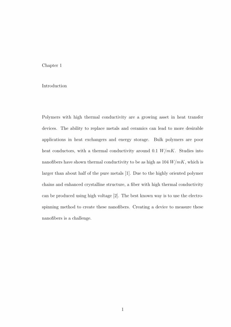
Polymers with high thermal conductivity are a growing asset in heat transfer
devices. The ability to replace metals and ceramics can lead to more desirable
applications in heat exchangers and energy storage. Bulk polymers are poor
heat conductors, with a thermal conductivity around 0.1 W/mK. Studies into
nanofibers have shown thermal conductivity to be as high as 104 W/mK, which is
larger than about half of the pure metals [1]. Due to the highly oriented polymer
chains and enhanced crystalline structure, a fiber with high thermal conductivity
can be produced using high voltage [2]. The best known way is to use the electro-
spinning method to create these nanofibers. Creating a device to measure these
nanofibers is a challenge.
1
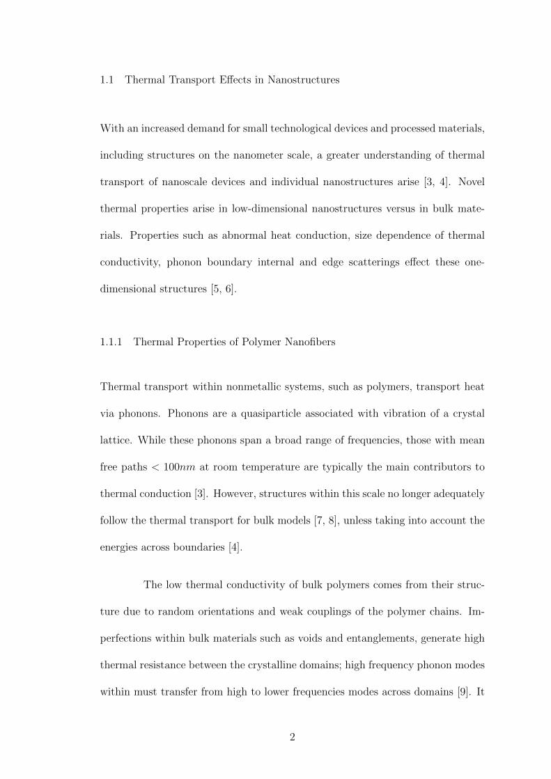
1.1 Thermal Transport Effects in Nanostructures
With an increased demand for small technological devices and processed materials,
including structures on the nanometer scale, a greater understanding of thermal
transport of nanoscale devices and individual nanostructures arise [3, 4]. Novel
thermal properties arise in low-dimensional nanostructures versus in bulk mate-
rials. Properties such as abnormal heat conduction, size dependence of thermal
conductivity, phonon boundary internal and edge scatterings effect these one-
dimensional structures [5, 6].
1.1.1 Thermal Properties of Polymer Nanofibers
Thermal transport within nonmetallic systems, such as polymers, transport heat
via phonons. Phonons are a quasiparticle associated with vibration of a crystal
lattice. While these phonons span a broad range of frequencies, those with mean
free paths < 100nm at room temperature are typically the main contributors to
thermal conduction [3]. However, structures within this scale no longer adequately
follow the thermal transport for bulk models [7, 8], unless taking into account the
energies across boundaries [4].
The low thermal conductivity of bulk polymers comes from their struc-
ture due to random orientations and weak couplings of the polymer chains. Im-
perfections within bulk materials such as voids and entanglements, generate high
thermal resistance between the crystalline domains; high frequency phonon modes
within must transfer from high to lower frequencies modes across domains [9]. It
2
has been found through many studies that polymer nanofibers with highly aligned
polymer chains can have much higher thermal conductivities and Young’s mod-
ulus than typical bulk values [1, 2, 3, 9, 10, 11]. As the degree of crystallinity,
increases so does the thermal conductivity [12, 13, 14]. Through techniques such
as the draw and electro-spinning methods, polymer chain alignments and crys-
tallinity can be enhanced. Attaining oriented and stretched polymer chains, as
well as increased crystal sizes, can enhance mechanical strength and adversely
affect thermal conductivity.
Zhong et al. were able to measure thermal conductivity of single Ny-
lon–11 nanofibers fabricated utilizing electro-spinning [9]. Using a micro-device
platform, the thermal conductivity of fibers between 50-400nm in diameter were
measured to be between 0.35 - 1.6 W/mK, compared to the bulk form, which
measured between 0.2 – 0.25 W/mK. Zhong was also able to measure the the
crystallinity using Wide-Angle X-ray Scattering (WAXS). This technique specif-
ically refers to the analysis of Bragg peaks scattered to wide angles (2θ > 1◦)
within sub-nanometer structures. They found the crystallinity to be ≈ 35%; how-
ever such measurements require a collection of fibers and cannot be utilized on
single fibers.
Studies by Yao and Papkov, Dimitry, et al. showed that the electro-
spinning method for producing such nanofibers suggested that since the process in-
volves rapid evaporation of the solvent, the subsequent solidification of nanofibers
inhibits polymer crystallization [15, 16]. This was suggested due to the relaxation
times and residual solvents remaining within after the fiber has been spun; this
can accelerate chain relaxation and lead to shorter relaxation times [17, 18]. This
3
can also be seen for polymers with high glass Transition temperature (Tg) values
[19]. However, with polymers and polyesters with lower Tg values, such as PCL
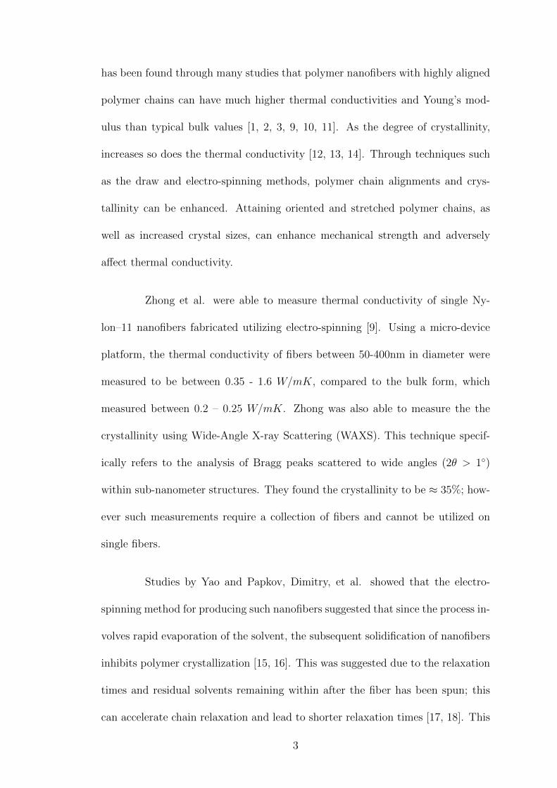
(Tg ∼ −60◦C), takes longer time to crystallize [20]. A gel-spinning process can
fix this dilemma by applying a post-drawing once the fiber is in solid state below
the melting temperature to prevent chain relaxation after orientation [21, 15]; the
design is seen in 1.1.
Figure 1.1: Design of the gel-spinning process [21]
A similar method to the gel-spinning process is the ultra-drawing method
which was utilized by Sheng Shen et al. in 2010. Shen fabricated and measured
the thermal conductivity of single polyethylene nanofibers showing an increase in
thermal conductivity compared to that of bulk polyethylene from 0.1 W/mK to
values as high as 104 W/mK [1]. These fibers ranged from 50 – 500nm diameters
and lengths up to tens of millimetres.
Despite these recent advancements in thermal conductivity enhancement
4
via drawing, there is still a lack of fundamental understanding of the relation-
ship between the structures and attained thermal transport properties in polymer
nanofibers.
1.2 Measurement Techniques
Much effort has gone into developing advanced thermal conductivity measurement
techniques. On more of a macro scale, there exists the 3w technique. This tra-
ditional method is meant to measure polymer thin films using an AC current at
frequency w through the sample leading to output voltage oscillations. The first
reported use of the 3w method to measure the thermal conductivity of solids was
by Cahill (Cahill and Pohl 1987). Cahill’s 3w technique utilizes a micro-fabricated
metal line that acts as a heater/thermometer. “When an alternating current (AC)
voltage signal is used to excite the heater at a frequency w, periodic heating gen-
erates oscillations in the electrical resistance of the metal line at a frequency of
2w. In turn, this leads to a third harmonic (3w) in the voltage signal, which is
used to infer the magnitude of the temperature oscillations” [22]. However, this
technique is difficult to implement on a single nano-structure.
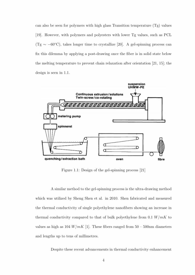
Another technique used a micro device that suspended carbon nanotubes
between two silicon nitrite plates. Current was passed through one generating a
heat input, where the induced temperature change was measured through the
other [23]. These plates were fabricated using an electron beam, photolithogra-
phy, metal coating, and etching. Each island consisted of a platinum thin film
resistor. This served as a heater to increase the temperature. Since the tempera-
5
ture changed with a change in their resistance, these could also be used to measure
the temperature of each island [24]. Carbon nanotubes were then bridged between
the two suspended islands using a similar method used to fabricate Atomic Force
Microscope (AFM) scanning probe tips. This technique is used throughout indus-
tries to measure the thermal conductance of carbon nanotubes. However, it is not
used for single polymer nanofibers.
Figure 1.2: Suspended Micro-device [24]
In more recent years two measurement methods were able to measure
the thermal conductivity of a single polymer nanofiber: Shen [1] and Canetta
[25]. Shen utilized a bi-material cantilever to directly draw a polymer wire from
a droplet from a soldering iron tip. Shen constructed an optical system within a
vacuum to measure the deflections from the bi-material cantilever once the tip of
the iron was heated, seen in Figure 1.3. A fiber thermal conductivity could be
known since the temperature of the heated tip and calculations of beam deflections
due to temperature changes were known.
6
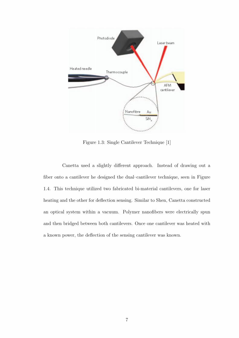
Figure 1.3: Single Cantilever Technique [1]
Canetta used a slightly different approach. Instead of drawing out a
fiber onto a cantilever he designed the dual–cantilever technique, seen in Figure
1.4. This technique utilized two fabricated bi-material cantilevers, one for laser
heating and the other for deflection sensing. Similar to Shen, Canetta constructed
an optical system within a vacuum. Polymer nanofibers were electrically spun
and then bridged between both cantilevers. Once one cantilever was heated with
a known power, the deflection of the sensing cantilever was known.
7

Figure 1.4: Duel Cantilever Technique [25]
1.3 Proposed Method
In combination with both Shen and Canetta’s designs, my novel design will use two
cantilevers in forced actuation, as seen in Figure 1.5. This design will take a look
at a new thermal conductivity measurement design that focuses on a mechanical
system rather than an optical method. The reason to create such a design is to
mitigate complexity in measuring polymer nanofibers by joining two independent
subsystems. This allows the underlining bi-material cantilever and fiber sample
to be easily loaded into a traditional AFM without modification or cost.
A sample plate, which is loaded into the AFM, includes a heated prong,
bi-material cantilever, and electro-spun nanofiber, where as the AFM will only
include a tipless silicon cantilever and operated normally. Both cantilevers will
be placed tip to tip, once temperature is added to the system, the temperature
sensitive bi-material cantilever will force the AFM’s cantilever to deflect. The
deflection will then be recorded, which will then be used to obtain the fibers
thermal conductivity. This will be known as the Probe-to-Probe Technique.
8
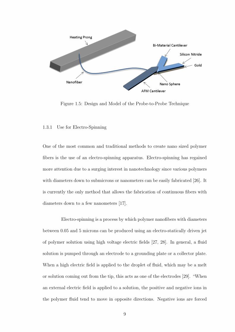
Figure 1.5: Design and Model of the Probe-to-Probe Technique
1.3.1 Use for Electro-Spinning
One of the most common and traditional methods to create nano sized polymer
fibers is the use of an electro-spinning apparatus. Electro-spinning has regained
more attention due to a surging interest in nanotechnology since various polymers
with diameters down to submicrons or nanometers can be easily fabricated [26]. It
is currently the only method that allows the fabrication of continuous fibers with
diameters down to a few nanometers [17].
Electro-spinning is a process by which polymer nanofibers with diameters
between 0.05 and 5 microns can be produced using an electro-statically driven jet
of polymer solution using high voltage electric fields [27, 28]. In general, a fluid
solution is pumped through an electrode to a grounding plate or a collector plate.
When a high electric field is applied to the droplet of fluid, which may be a melt
or solution coming out from the tip, this acts as one of the electrodes [29]. “When
an external electric field is applied to a solution, the positive and negative ions in
the polymer fluid tend to move in opposite directions. Negative ions are forced
9
toward the positive electrode, and positive ions are forced toward the negative
electrode [19].” This leads to the droplet deformation and finally to the ejection
of a charged jet from the tip of the cone accelerating towards the counter electrode
leading to the formation of continuous fibers [30, 31].
At a traditional needle tip where the droplets or strands are produced,
a Taylor Cone is formed. This is a consequence of electrical forces that form a
conical protrusion [19, 32]. This theory was first described by Taylor in 1964 [33].
As charged liquid is pumped out of the needle, surface tension keeps the droplet
appended until the surface charges of the droplet are overcome by the grounding
electrode. As the intensity of the electric field is increased, the hemispherical
surface of the fluid at the tip of the needle elongates to form a conical shape
known as a Taylor Cone. Taylor studied these electric fields E and their influence
on surface tension σ,
1
2εoE
2 =σ
r tanα(1.1)
where εo is the permittivity of free space (Fm−1), r tanα is the curvature
of a cone, and α is the half cone angle [34, 35]. He predicted that it only took
an angle of 49.3◦. However, Taylor’s Cone angle should be 33.5◦ instead of 49.3◦,
as reported from Yarin et al (2001) [26], due to the Taylor Cone being a specific
self-similar solution, meaning a flow which ’looks the same’ either at all times or
at the same scale. Moreover, there do exist non-self-similar solutions that do not
tend toward a Taylor Cone [36]. The surface tension, viscoelasticity, and charge
density within the ejected polymer are the key influences in proper fiber formation
[37].
10
The discharged liquid solution jet undergoes an instability and elongation
process, which allows the jet to become long and thin. Meanwhile, the solvent
evaporates, leaving behind a charged polymer fiber. In the case of the melt, the
discharged jet solidifies when it travels in the air [26]. The discharged polymer
solution jet undergoes a whipping process wherein the solvent evaporates, leaving
behind the charged polymer fiber, which tends to the grounding plate [28].
1.3.2 AFM Use
The Atomic Force Microscope (AFM/SFM) is within the family of the Scanning
Probe Microscopes (SPMs). Other probe microscopes, such as Scanning Tunnel-
ing Microscopy (STM) or Scanning Near-field Optical Microscopes (SNOM) focus
on quantum tunneling and short range electromagnetic fields, which are not useful
with this proposed research [38]. An AFM utilizes force interactions to measure
the structure of roughness of a surface. The instrument is able to collect informa-
tion on the arrangement of individual molecules and even individual atoms in a
sample with high accuracy and detailed resolution [39]. AFMs are useful for mea-
suring magnetic fields, friction gradients, peizo response, temperature, nanoscale
forces, and elasticity of samples. Additional surface characterization techniques
such as Scanning Electron Microscopes (SEMs), allow for resolutions of about 25
Angstroms utilizing an electron beam rather than a light source [40]. However,
polymers exhibit weak electron scattering and poor contrast and act essentially
like organic materials within this system. Secondly, polymers typically have low
electrical conductivity leading to rapid accumulation of negative charges, which
dramatically decreases resolution [41]. SEMs may also damage polymers due to
11
their high power; AFMs only utilize the inter-atomic forces, a non-destructive tech-
nique for surface measurements [42]. The AFM will be used based on its ability
to detect the small temperature-mechanical displacement variations implemented
into the system and utility compared to previously mentioned instruments.
AFM Components
The main components of an AFM consist of a cantilever probe, piezoelectric scan-
ner, force sense, laser, Proportional Integral and Derivative (PID) controller, and
a photo diode signal detector, as seen in Figure 1.6 [43]. A probe is attached to a
cantilever beam that is used to read the roughness of a surface as the probe scans
in XY coordinates and interacts with the sample. As the cantilever is deflected
due to forces exerted from the sample, a focused laser senses this change and sends
a signal to the photo-diode detector. Once the detector notices this change, either
the piezo stage moves to counter at the variation or stays static and records the
bending moment, depending on the mode type.
12
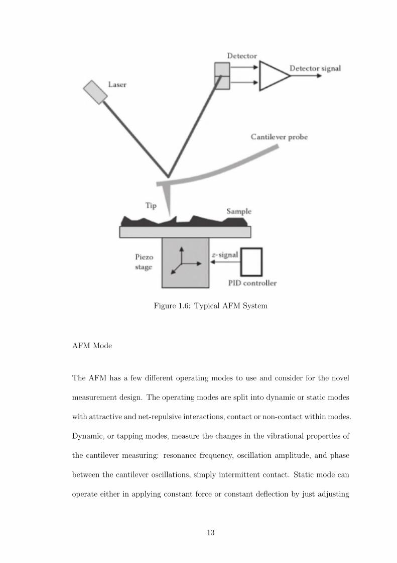
Figure 1.6: Typical AFM System
AFM Mode
The AFM has a few different operating modes to use and consider for the novel
measurement design. The operating modes are split into dynamic or static modes
with attractive and net-repulsive interactions, contact or non-contact within modes.
Dynamic, or tapping modes, measure the changes in the vibrational properties of
the cantilever measuring: resonance frequency, oscillation amplitude, and phase
between the cantilever oscillations, simply intermittent contact. Static mode can
operate either in applying constant force or constant deflection by just adjusting
13
the z-piezo axis of the cantilever. However, in this case, since the sample will not
be moving nor have the need for vibrational properties and the need for variable
force change, the design will use a net-repulsive contact static mode, non-vibrating
mode. The system will be held at a constant position and not allow the cantilever
to re-position once deflection is noticed.
AFM System Parameters
Without constructing an external optical system as seen in prior designs, AFMs
are programmed to be optimized, adjusted, and calibrated to certain preferences.
This allows the PID gains controller and High Voltage (HV) gains of the system
piezos to adjusted to particular parameters, depending on the need.
A sample is typically fixed on the top of a 3-axes piezoelectric stage that
moves the sample under the tip, where the movements X and Y are controlled by
the computer that generates two synchronized voltage ramps (gains) [44]. Once in
contact, a force transducer sensor senses the force between the tip and the surface,
allowing the feedback controller to feed a signal from the transducer back to the
piezoelectric stage. This allows the AFM to maintain a fixed force between tip
and sample. Typically, the expansion coefficient for a single piezoelectric device
is on the order of 0.1nm per applied volt. Therefore, if the voltage to excite the
piezoelectric stage is 2 volts, then the material will expand about 0.2nm [39].
The z-piezoelectric stage and the force transducer are linearly mirrored.
Therefore to get the most data out of the AFM in use (can only record two devices
at once), the XY piezo gains and force transducer gain will be zeroed. Zeroing
14
the transducer gains allows the piezo stage not to respond to photo-diode signals.
Secondly, turning off the X and Y piezo stage gains hinders the scanning in X and
Y directions, but still allows sensing detection from the photo-diode. Additionally,
the PID gain controls can also be adjusted to scale the system properly, such that
the feedback loop will respond quickly to topography changes. More on these
settings will be discussed in Chapter 4.
1.3.3 Use of Bi-Material and Silicon Cantilevers
The reason for using a bi-material cantilever is because it has high sensitivity
due to small dimensions and thermal mass [45]. A bi-material cantilever beam is
comprised of two material layers. Typically bi-material cantilevers are made of
silicon and coated with gold or aluminum to improve reflectively for AFM sensing.
Once a temperature change is introduced, the cantilever will deflect due to the
difference in Coefficients of Thermal Expansion (CTE) of both layers. These
types of bi-material cantilevers have shown the ability to detect deflections at 3
pm resolution with the measurement of temperature, optical power, and energy
with 2 µK, 76 pW , and 15 fJ resolution, respectively [46].
Typical silicon heated cantilevers have spring constants ranging from
0.01 to 10 N/m, and resonant frequencies ranging from 50 to 300 kHz and are
calibrated using the thermal noise method [47]. Raman microspectroscopy char-
acterizes them with spatial and temperature resolutions of 1 µm and 3◦C [47, 48].
Additional research of laser heated cantilevers, shows that contact thermal con-
ductivity is typically in the range 0.1–100 nW/mK; and for probe tip radii of 30
15
nm, a typical contact diameter is about 10 nm providing a contact force of 10 nN.
The spreading contact conductivity due to 10 nm contact on a polymer sample
becomes 2 nW/mK [48]. This may be useful when determining conductivity of
the cantilevers utilized within this thesis.
Furthermore, the heat transfer coefficient air gap hairgap may be noticed
when determining heat transfer from fiber to cantilever. As seen in equation 1.2,
the hairgap would be on the order of 10 kW/m2K for a tip height of 1–10 µm.
Similarly, the probe being utilized within this thesis has a 15µm diameter. In
continuing works, this may be useful. Moreover, 10 kW/m2K will also be utilized
for the heat transfer coefficient for the fiber.
hairgap =kaird
(1.2)
More on the properties of the cantilevers can be seen in the Appendix.
1.4 Thesis Outline
The purpose of this thesis is to further understand the thermal effects and conduc-
tivity capabilities of polymer nanofibers and to supply a novel method of measure-
ment to the research community. With the use of temperature sensitive bi-material
cantilevers and AFMs, one can obtain the thermal conductivity of electro-spun
nanofibers.
Chapter 2 reviews introductory thermodynamics, along with the theoret-
16
ical design of the Probe-to-Probe measurement system. This design incorporates
a two cantilever force interactive relationship. The reason to create such a design
is to mitigate complexity in the measurement of polymer nanofibers by joining
two independent subsystems. This allows the underlining bi-material cantilever
and fiber sample to be easily loaded into a traditional AFM without modification
or cost. Detailed modeling of this conjoined system design can be seen here.
Chapter 3 focuses on the experimental apparatus, fiber creation, and
equipment used. It will review the electro-spinning apparatus used for fiber fab-
rication, the experimental setup and creation of sample plates, fiber appending,
measurement and alignment, and AFM integration for the measurement process.
Chapter 4 describes the procedural measurement of the system and out-
lines how the system was calibrated, along with how each of the system settings
was determined.
Chapter 5 details all the results from testing, including: natural de-
flections, pre-appended fiber calibrations, and appended fiber recordings. Each
review incorporates findings and comparisons of measured results to theoretical
expectations, along with explanations and discussions.
Chapter 6 provides a summary of descriptions and conclusions from each
chapter, along with a discussion of what can be done in future experiments to
provide expected results.
17
Chapter 2
Design and Modeling
This chapter will review introductory heat transfer and the thermal modeling of
the system in use. As seen in figure 1.5 the system utilizes a heating prong, a
silicon tipless AFM cantilever, and a bi-material AFM cantilever. As heat is sent
through the base of the heating prong it is transferred through the fiber to the tip
if the bi-material cantilever. Due to the thermal expansion of gold verse silicon
nitride, the gold deflects and adversely bends the tipless AFM cantilever. The
AFM cantilever deflects, and the laser from the AFM records this beam deflection.
As seen from natural beam deflection theory and Hooke’s Law this deflection can
be used to obtain the temperature output Tct from the fiber at the tip of the bi-
material cantilever. In congruence, the flux qf and temperature Tf into the fiber
from the heating prong is obtained through the use of thermocouples. The thermal
conductivity of the nanofiber kf can be found after finding the temperatures at
both ends of the fiber.
The system will be modeled as a one-dimensional time-independent steady
state problem. This allows the modeling and measurements to be simplified. Sub-
scripts p, f , and c, and directions x1, x2, and x3 represent the prong, fiber, and
18
bi-material cantilever respectively throughout this paper.
2.1 Heat Transfer and Conduction
Before reviewing the thermal models through the proposed system, the first step
it to briefly explain heat transfer fundamentals for one-dimensional systems. Heat
transfer by conduction is the flow of thermal energy within a solid and non-flowing
fluids driven by a non-uniform temperature field. Heat transfer Q and work W are
the two types of energy interactions that make up the internal energy E. These
interactions are known as the first Law of Thermodynamics for a closed system or
the conservation of energy:
∂E = Q−W (2.1)
Internal energy is associated with the disorderly motion of molecules transferring
kinetic and potential energies, where heat is transferred by conduction. Work is
the transfer of energy resulting from a force acting through a distance and heat
is the energy transferred as the result of a temperature difference [49]. In terms
of unidirectional and per-time equivalent through a insulated beam with heat
generation from equation 2.1, internal energy can be simplified as
∂E
∂t= Qin −Qout +W (2.2)
or
∂E
∂t= Aqx − Aqx+∆x +W (2.3)
as a heat transfer rate q with some output change ∆x in terms of heat
19
flux qx = Q/A (W/m2). This is also known as Fourier’s Law of heat conduction
which reads
qx(x, t) = −k∇T (x, t) (2.4)
where k is the thermal conductivity and ∇T is the temperature gradient [50].
This is the assumption that the material is isotropic and homogeneous where the
thermal conductivity is constant.
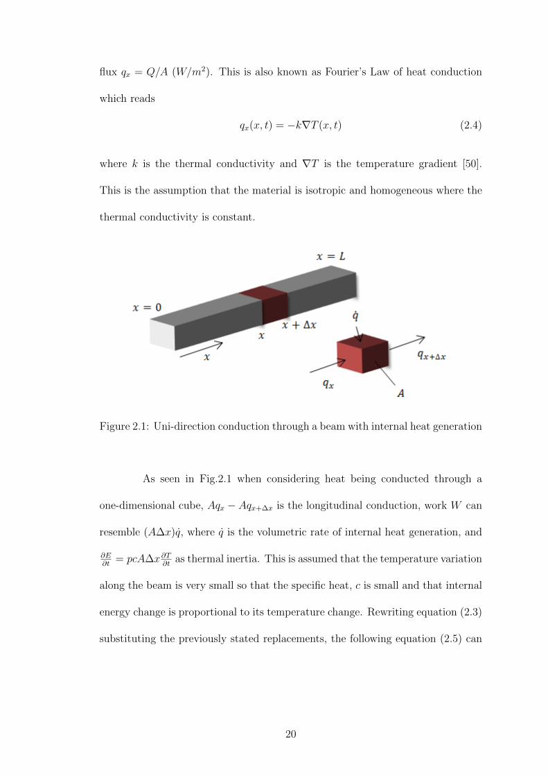
Figure 2.1: Uni-direction conduction through a beam with internal heat generation
As seen in Fig.2.1 when considering heat being conducted through a
one-dimensional cube, Aqx − Aqx+∆x is the longitudinal conduction, work W can
resemble (A∆x)q, where q is the volumetric rate of internal heat generation, and
∂E∂t
= pcA∆x∂T∂t
as thermal inertia. This is assumed that the temperature variation
along the beam is very small so that the specific heat, c is small and that internal
energy change is proportional to its temperature change. Rewriting equation (2.3)
substituting the previously stated replacements, the following equation (2.5) can
20
be re-solved as the thermal inertia.
pcA∆x∂T
∂t= Aqx − Aqx+∆x + A∆xq (2.5)
However, this equation takes into account non-steady state with internal heat
generation. Since the modeling and experimentation require steady state and
there exists zero internal heat generation, the internal energy equation reduces to
only terms of conduction. Simplifying equation 2.5 and substituting Fourier’s Law
2.4 in x-direction obtains equation 2.6 called heat conduction, to be utilized later.
Qcond = Aqx − A(qx +∂qx∂x
∆x) (2.6)
2.2 Thermal Modeling of a Fin
For both 1D beams and rods, or cantilevers and fibers respectively, the heat trans-
fer through these systems can be modeled as fins including Newtons Law of Cool-
ing. Steady state is defined as the process of unchanging time which will be
considered zero since the collection of experimental data will be assumed to be
steady state. The heat generated term will be considered the heat sink for cooling
fins. Reviewing equation 2.5 and noting that in steady state all the heat that is
being generated inside the fins must be transferred to the fluid around the fin,
in this case the fluid is air. The temperature distribution T (x) reaches a steady
state because the surface of the fins are bathed in an ambient temperature T∞
where the heat transfer coefficient h is uniformly surrounding the perimeters P by
21
a change of length ∆x. As seen in equation 2.7 the lateral heat convection can be
written:
Qconv = −Ph∆x(T (x)− T∞) (2.7)
The fins can be modeled as 1D because the conduction through the axis
the y and radial directions respectively are much lower than in the lengths of each
model. Using the dimensionless quantity of the Biot number, the thermal contact
of the surface of the fins to the fluid can be shown to be ’poor’, or that the fins
are good thermal conductors. If the Biot number in equation 2.8 is << 1 over
the length of the fin, than the boundary temperature is nearly the same as the
temperature in the center of the fin. A typical AFM cantilever has a Boit number
less than 10−4, confirming it can be modeled as 1D [48, 51]. This also works for
each subsystem (prong, fiber, and both cantilevers).
Bi =hL
k(2.8)
Again with assuming steady state and that each part of the system is modeled as
individual fins, the heat balance for each fin problem will be similar. Combining
equations 2.6 and 2.7 the heat balance equation becomes:
Aqx − A(qx +∂qx∂x
∆x)− Ph∆x(T (x)− T∞) = 0 (2.9)
Taking the lim∆x→0, equation 2.9,:
lim∆x→0
A∂qx∂x− Ph(T (x)− T∞) = 0 (2.10)
22
Then substituting the modified Fourier Law as heat flux and taking the derivative
with respect to x gives:
qx = −k∂T∂x
→ ∂qx∂x
= −k∂2T (x)
∂x2(2.11)
Combining equations 2.10 and 2.11 the governing equation of a fin be-
comes:
∂2T (x)
∂x2−m2(T (x)− T∞) = 0 (2.12)
where
m2 =Ph
Ak(2.13)
The constants m, P , and A will represent the perimeters and cross sectional area
respectively in each of the three fin systems. For the heating prong and bi-material
cantilever the perimeter P = w + s and the area A = ws, where w and s are the
width and thickness respectively. For a fiber it is modeled as a cylinder so Pf = πd
and Af = π(d2)2, where d is the measured diameter of the fiber. Therefore the
general solution temperature profile of a fin is equation 2.14 where Ca and Cb will
represent variable constants, a and b represent multiple constants.
T (x) = Cae−mx + Cbe
mx + T∞ (2.14)
This will be utilized throughout modeling each fin. After the boundary conditions
are defined, the constants can be found.
23
2.3 Thermal Modeling of the Heating Prong
When it comes to appending a fiber to the system it is difficult to get it directly
in the same position along the heating prong every time a new fiber is added. The
best method is to theoretically model the flux at any point to the fibers position
on the prong. Since the fiber can sit anywhere along the prong, the heat flux,
temperature, and length to the fiber from the base, all vary. As seen in Figure.
2.2 the equation
Qf (x2) = Qp1(x1)−Qp2(x1)⇒ Afqf (x2) = Apqp1(x1)− Apqp2(x1) (2.15)
or
kf∂Tf (x2)
∂x2
= kp∂Tp1(x1)
∂x1
− kp∂Tp2(x1)
∂x1
(2.16)
can be used to measure the heat flux at any position where qf (x2) is the flux into
the fiber, qp1(x1) is the input flux at the fiber location on the prong and qp2(x1) is
the output flux to the rest of the prong. In this case Af = Ap since fluxes in the
contact cross sectional areas are the same. Since flux into the fiber is represented
from equation 2.15, a change in temperature along the fiber will also need to be
found. Equation 2.16 is the general form in which to solve for kf .
24
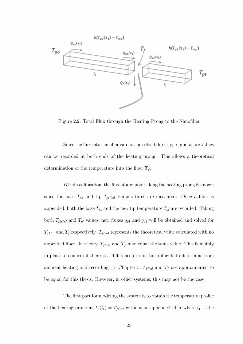
Figure 2.2: Total Flux through the Heating Prong to the Nanofiber
Since the flux into the fiber can not be solved directly, temperature values
can be recorded at both ends of the heating prong. This allows a theoretical
determination of the temperature into the fiber Tf .
Within calibration, the flux at any point along the heating prong is known
since the base Tpo and tip TptCal temperatures are measured. Once a fiber is
appended, both the base Tpo and the new tip temperature Tpt are recorded. Taking
both TptCal and Tpt values, new fluxes qp1 and qp2 will be obtained and solved for
TfCal and Tf respectively. TfCal represents the theoretical value calculated with no
appended fiber. In theory, TfCal and Tf may equal the same value. This is mainly
in place to confirm if there is a difference or not, but difficult to determine from
ambient heating and recording. In Chapter 5, TfCal and Tf are approximated to
be equal for this thesis. However, in other systems, this may not be the case.
The first part for modeling the system is to obtain the temperature profile
of the heating prong at Tp(l1) = TfCal without an appended fiber where l1 is the
25
length from the base of the prong to the fiber. From equation 2.14, Tp(x1) is
represented as,
Tp(x1) = C1e−mpx1 + C2e
mpx1 + T∞p. (2.17)
Utilizing boundary conditions:
Tp(0) = Tpo (2.18)
Tp(l1 + l2) = TptCal (2.19)
Solving for constants C1 and C2:
C1 = (Tpo − T∞p)− C2 (2.20)
C2 =(TptCal − T∞p)− (Tpo − T∞p)e
−mp(l1+l2)
2sinh(mp(l1 + l2))(2.21)
Combining equation 2.17 and constants C1 and C2 at Tp(l1) = TfCal and
re-writing the profile in terms of TfCal becomes:
TfCal = [(TptCal−T∞p)sinh(mpl1)+(Tpo−T∞p)sinh(mpl2)]csch(mp(l1 + l2))+T∞p
(2.22)
Again this temperature value is represented as the heat flux qp1 at any temperature
TfCal along the heating prong.
26
2.3.1 Heating Prong Fluxes qp1(x1) and qp2(x1)
Obtaining fluxes qp1 and qp2 are the next steps to solving the thermal conductivity
of a single nanofiber using equation 2.16. To find both fluxes qp1 and qp2, the
temperature profiles will be split into two separate systems as seen in Figure 2.2.
Again, the Tf obtained here will be compared with the TfCal to show similarity.
Heating Prong Flux, qp1(x1):
The governing equation can be written as:
∂2Tp1(x1)
∂x21
−m2p(Tp1(x1)− T∞p) = 0 (2.23)
where the temperature profile from equation 2.14 becomes
Tp1(x1) = C3e−mpx1 + C4e
mpx1 + T∞p (2.24)
Utilizing boundary conditions:
Tp1(0) = Tpo (2.25)
Tp1(l1) = Tf (2.26)
After applying boundary conditions, the constants are found to be:
C3 = (Tpo − T∞p)− C4 (2.27)
27
C4 =(Tf − T∞p)− (Tpo − T∞p)e
−mpl1
2sinh(mpl1)(2.28)
Combining equations 2.16 and 2.3.1, and rearranging the constants solv-
ing for qp1(l1) gives:
qp1 = −kp∂Tp1(l1)
∂x1
= kpmp[(Tf −T∞p)coth(mpl1)− (Tpo−T∞p)csch(mpl1)] (2.29)
Heating Prong Flux, qp2(x1):
The flux from the second part of the prong is similarly solved as qp1 however, with
reverse direction. Referencing back to Figure 2.2 and equation Tp2(x1) governing
equation can be written as:
∂2Tp2(x1)
∂x21
−m2p(Tp2(x1)− T∞p) = 0 (2.30)
where the temperature profile becomes
Tp2(x1) = C5e−mpx1 + C6e
mpx1 + T∞p (2.31)
Applying boundary conditions:
Tp2(0) = Tpt (2.32)
Tp2(l2) = Tf (2.33)
28
Again this tip temperature Tpt is when a fiber is appended. The temperature
exiting and entering into the second portion of the prong and fiber should all be
the same temperature TfCal. After applying boundary conditions constants are
found to be:
C5 = (Tpo − T∞p)− C6 (2.34)
C6 =(Tf − T∞p)− (Tpt − T∞p)e
−mpl2
2sinh(mpl2)(2.35)
Combining equations 2.16 and 2.31, and rearranging the constants solv-
ing for qp2(l2) gives:
qp2 = kp∂Tp2(l1)
∂x1
= −kpmp[(Tf −T∞p)coth(mpl2)− (Tpt−T∞p)csch(mpl2)] (2.36)
2.3.2 Thermal Modeling of a Single Nanofiber
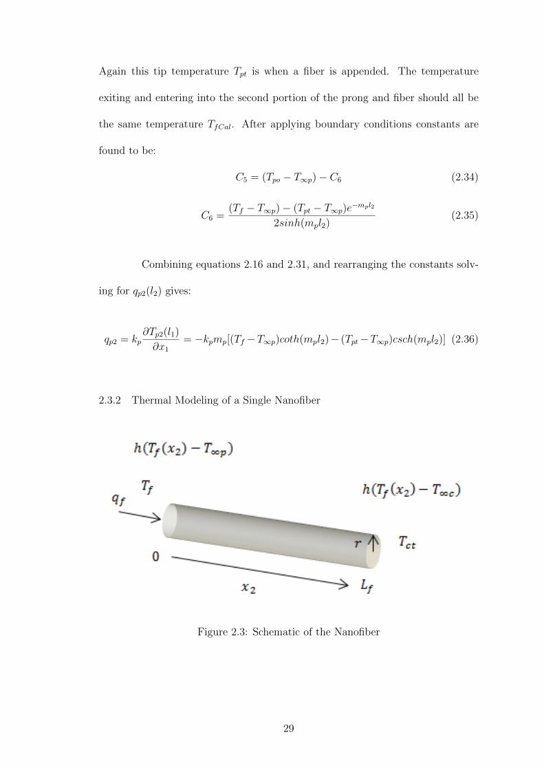
Figure 2.3: Schematic of the Nanofiber
29
The next step is to find the temperature profile of the nanofiber as seen in Fig-
ure 2.3. The modeling of the fiber is similar to a traditional 1D fin problem,
however, there is an additional ambient temperature change over the length of
the fiber. This can be measured, seen in calibration from the prong to the bi-
material cantilever. Therefore the change of ambient temperature was treated as
a linear decline since T∞p at the prong has a higher temperature than T∞c at the
cantilevers. The governing equation of Tf (x2) including T∞(x2) is written as
∂2Tf (x2)
∂x22
−m2fTf (x2) = −mfT∞(x2) (2.37)
Since T∞(x2) is similar to a forcing function for this second order non-homogeneous
differential equation, the temperature profile Tf (x2) will have to be split into a
homogeneous and particular solutions [52]. Using
y = yh + yp (2.38)
where y = Tf (x2), yh is the homogeneous solution, and yp is the particular solution.
The solution to the homogeneous solution of the temperature profile is
yh = C7e−mfx2 + C8e
mfx2 (2.39)
when yp = 0, which is similar to that of previous fin solutions. Allowing T∞(x2)
to be a linear function represented as
T∞(x2) = C9x2 + C10 (2.40)
30
Referencing Figure 2.3 the boundary conditions are:
T∞(0) = T∞p (2.41)
T∞(Lf ) = T∞c (2.42)
where constants C9 and C10 can be simply solved as
C9 =T∞c − T∞p
Lf
(2.43)
C10 = T∞p (2.44)
The particular equation solution reduces to:
yp = C9x2 + C10 (2.45)
Adding the homogeneous equation 2.39 and particular 2.45 solutions to obtain
equation 2.46, keeping C9 and C10 for simplification.
Tf (x2) = C7e−mfx2 + C8e
mfx2 + C9x2 + C10 (2.46)
After applying boundary conditions:
Tf (0) = Tf (2.47)
Tf (Lf ) = Tct (2.48)
31
C7 and C8 can be found:
C7 = (Tf − T∞p)− C8 (2.49)
C8 =(Tct − T∞c)− (Tf − T∞p)e
−mfLf
2sinh(mfLf )(2.50)
Using equation 2.46 and substituting constants 2.49, 2.50, 2.43, 2.44 and
solving equation 2.15 for qf = −kf ∂Tf (0)
∂x2, qf is
qf = kfmf [(Tf−T∞p)coth(mfLf )−(Tct−T∞c)csch(mfLf )+(T∞p − T∞c)
mfLf
] (2.51)
Now that all the fluxes of equation (2.15) have been obtained, all but the thermal
conductivity of the fiber kf and the tip temperature of the bi-material cantilever
Tct are known.
2.4 Applied Temperature with AFM Integration
Since flux into the fiber is represented from equation 2.15, all the fluxes 2.29, 2.36,
and 2.51 have been solved. Next is to obtain the output temperature Tct to be
substituted into equation 2.51 where the thermal conductivity kf of the fiber can
be found. This temperature is found through the bi-material cantilever deflection
with an applied force at the tip. The applied force is due to the resistance from the
above AFM cantilever; the natural beam deflection, where only thermal expansion
is acting on it. Since the natural bi-material deflection is a function of the tem-
perature profile Tc(x3) the next set of modeling will be split into three sections:
temperature profile, natural beam deflection, and acting force displacement from
Hooke’s Law.
32
2.4.1 Bi-Material Cantilever Temperature Profile
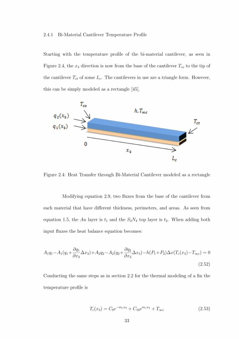
Starting with the temperature profile of the bi-material cantilever, as seen in
Figure 2.4, the x3 direction is now from the base of the cantilever Tco to the tip of
the cantilever Tct of some Lc. The cantilevers in use are a triangle form. However,
this can be simply modeled as a rectangle [45].
Figure 2.4: Heat Transfer through Bi-Material Cantilever modeled as a rectangle
Modifying equation 2.9, two fluxes from the base of the cantilever from
each material that have different thickness, perimeters, and areas. As seen from
equation 1.5, the Au layer is t1 and the S3N4 top layer is t2. When adding both
input fluxes the heat balance equation becomes:
A1q1−A1(q1+∂q1
∂x3
∆x3)+A2q2−A2(q2+∂q2
∂x3
∆x3)−h(P1+P2)∆x(Tc(x3)−T∞c) = 0
(2.52)
Conducting the same steps as in section 2.2 for the thermal modeling of a fin the
temperature profile is
Tc(x3) = C9e−mcx3 + C10e
mcx3 + T∞c (2.53)
33
where m2c was solved when the width was much greater than the thickness t:
m2c =
2h
k1t1 + k2t2(2.54)
Utilizing the boundary conditions
Tc(0) = Tco (2.55)
Tc(Lc) = Tct (2.56)
the constants are solved as:
C11 = Tco − T∞c − C12 (2.57)
C12 =(Tct − T∞c)− (Tco − T∞c)e
−mcLc
2sinh(mcLc)(2.58)
where the complete temperature profile of the bi-material cantilever is:
Tc(x3) = [(Tct−T∞c)− (Tco−T∞c)e−mcLc ][
sinh(mcx3)
sinh(mcLc)] + (Tco−T∞c)e
−mcx3 +T∞c
(2.59)
2.4.2 Bi-Material Natural Beam Deflection Theory
This section will cover a bi-material natural beam deflection when there is no force
added to the tip of the cantilever. In the below equations, three assumptions were
made. One is that a linear strain distribution existed through the thickness of
the beam, second that both materials are perfectly bonded at the interface, and
34
third, that the temperature distribution within the cantilever is uniform. Upon
temperature change, the bi-material cantilever will deflect due to the bending
moment generated by thermal expansion (a) of the two materials. As seen similarly
from Shen et al. the natural beam deflection equation can be written as equation
2.60 [53, 54, 45, 55]. From beam theory, the bending moment is related to the
moment of inertia multiplied by Young’s Modulus and the curvature radius of the
beam [56], where the double derivative is relevant to this curvature.
∂2znat∂x2
3
= N(Tc(x3)− To) (2.60)
where
N =6(a2 − a1)(t1 + t2)
t22G(2.61)
and
G = 4 + 6t1t2
+ 4(t1t2
)2 +E1
E2
(t1t2
)3 +E2
E1
t2t1
(2.62)
where E is Young’s Modulus and To is the temperature at which the
cantilever has zero deflection throughout, ∂2znat
∂x23
= 0 [57]. Since the cantilever has
the fixed and free end boundary conditions, below only considers the fixed end
where the slope and deflection are zero.
znat(0) = 0 (2.63)
∂znat(0)
∂x3
= 0 (2.64)
Integrating equation 2.60 with the temperature profile equation 2.59 and applying
35
boundary equation 2.64 the first constant d1 can be found as
d1 =N
mc
[(Tco − T∞c)coth(mcLc)− (Tct − T∞c)csch(mcLc)] (2.65)
Integrating again using equation 2.63, d2 is
d2 = − N
m2c
(Tco − T∞c) (2.66)
Instead of writing out the the deflection at some z(x3) since only the deflection at
the free end of the cantilever is needed, the full equation at znat(Lc) becomes:
znat(Lc) =N
m2c
(Tct−Tco)(1−mccsch(mcLc)+N
m2c
(Tco−T∞c)mcLccoth(mcLc)+NL2
c
2(T∞c−To)
(2.67)
This is the general form however, this model can be reduced when Tco = T∞c to
equation 2.68. This assumption can be made since in this case the cantilever has
non-uniform temperature distribution due to the heat at the tip of the cantilever.
This non-uniformity can be kept small from the temperature output of the fiber
[53].
znat(Lc) =N
m2c
(Tct − T∞c)(1−mccsch(mcLc)) +NL2
c
2(T∞c − To) (2.68)
This deflection is only taking into account a natural beam deflection with
no applied force at the free end. Solving equation 2.68 for Tct simplifies to:
Tct =m2
c
(1−mccsch(mcLc))[znatN− L2
c
2(T∞c − To)] + T∞c (2.69)
36
2.4.3 AFM Displacements
Individual Zero Deflection
Before discussing forced beam deflection, the individual AFM cantilevers in use
will be reviewed to obtain a To value. Again this value is temperature at which
there is zero deflection, which is more complex to find depending on the cantilever
in question considering each cantilever has an individual intrinsic bending moment.
If referring to a basic Pyrex-Nitride Probe (PNP) cantilever, which are probes
that have silicon nitride cantilevers with very low force constants, then these are
optimized for a bending less than 2◦ at room temperature for a long cantilever, a
100um will be less theoretically, as referenced by NanoAndMore USA Corp. But
due to the fact that nitride and gold have different thermal expansion coefficients
each cantilever has an individual zero deflection on a different temperature and
drift as a function of temperature.
The cantilever bending angle is the angle between the tangent to the
cantilever at its free end (tip) and the support chip surface in degrees. A positive
algebraic sign a is used for bending towards the detector side and a negative sign
for bending towards the tip side. A rough estimation of the bending angle may
be calculated from the cantilever length l and the total deflection h; this is only
valid for small angles.
|a| = 2 arctanh
l(2.70)
This may be useful when dealing with the calibration seen in Chapter 4,
37
however if a 2◦ or larger angle was to be used in a theoretical case, the deflection
determined can be subtracted from final displacements. However, we can assume
that since AFM cantilevers are optimized to have near zero deflection in room
temperature, this small angle will be considered zero deflection at room temper-
ature. So 23◦C, which is a standard scientific value of room temperature, will
be used for To throughout calibrations and measurements. Moreover, To may be
optimized in calibration, dropping to zero, since all temperatures will be zeroed
for simplification.
Forced Beam Deflection
As seen in Chapter 4 when the system is calibrated, the AFM cantilever will inter-
act with the bi-material cantilever. Both cantilevers will interact at the horizontal
plan with the AFM cantilever fixture tilt at 10 degrees. In calibration, the can-
tilevers will undergo two different forces. The first force interacts in less than a
few angstroms, this is known as the repulsive force. This results from a charge
overlap between both cantilever tips. This force is very localized, and involves only
a few near field interacting atoms. The other force is up to hundreds of angstroms
known as the attractive force, called the van der Waals (vdW) force. This results
from a change in dipole moment induced interaction [58, 59]. In calibration it can
be seen that these cantilevers can be adjusted to account for these forces. The
assumption can be made when knowing the ’jump-to-contact’ distance an addi-
tional jog on the AFM can be applied to infer that the net force on the system
can be zeroed and both cantilevers attend to a horizontal plane again minimizing
large angle deformations.
38
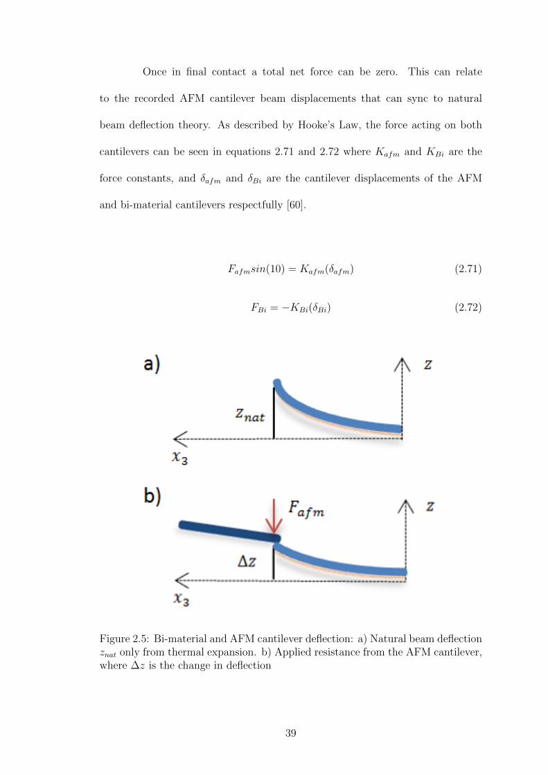
Once in final contact a total net force can be zero. This can relate
to the recorded AFM cantilever beam displacements that can sync to natural
beam deflection theory. As described by Hooke’s Law, the force acting on both
cantilevers can be seen in equations 2.71 and 2.72 where Kafm and KBi are the
force constants, and δafm and δBi are the cantilever displacements of the AFM
and bi-material cantilevers respectfully [60].
Fafmsin(10) = Kafm(δafm) (2.71)
FBi = −KBi(δBi) (2.72)
Figure 2.5: Bi-material and AFM cantilever deflection: a) Natural beam deflectionznat only from thermal expansion. b) Applied resistance from the AFM cantilever,where ∆z is the change in deflection
39
By forcing the system to be stationary when the cantilevers are in contact
the net force is zero [60], we can see that the displacement of one adversely affects
the other as
δBi =Kafm
KBisin(10)δafm (2.73)
Now that Hooke’s Law has been applied it must be referenced back to
natural beam deflection to obtain Tct needed considering a change of temperature.
When calibrated, natural beam deflection is already occurring. As seen in Figure
2.5, we can see that
δafm = znat − δBi (2.74)
where the difference from natural deflection to the displaced bi-material beam is
equivalent to the change in displacement from the AFM cantilever [61]. When a
force is applied from varied temperature of the bi-material cantilever to the AFM
cantilever a change in δafm occurs, dδafm, where additionally znat changes, dznat.
This dδafm change is the recorded displacement form the AFM photo-diode laser.
Both these values will be compared later after obtaining calibrated and appended
fiber measurements for zeroing and acquiring the Tct value. Combining equations
2.73 and 2.74 for znat in terms of the recorded displacement value δafm gives
znat = δafm[Kafm
KBisin(10)+ 1] (2.75)
Utilizing both equations 2.69 and 2.75 will give the temperature value
Tct needed to implement back into equation 2.51.
40
Chapter 3
Experimental Apparatuses
This chapter will review the electrospinning apparatus used for fiber fabrication,
the experimental setup of sample plates, and AFM integration for the measure-
ment process.
41
3.1 Sample Plates
3.1.1 Plate Design
A transitioning device and system play a key role to measure the thermal con-
ductivity of a single nanofiber. Thermally sensitive commercially obtained bi-
material cantilevers have been shown to successfully measure and conduct poly-
meric nanofibers [62]. In addition to their abilities, they are traditionally used in
nano-instrumentation as actuators and sensors [63]. AFM’s are typically useful in
measuring small optical cantilever beam deflections and are able to detect these
small thermal changes. However, with the use of an AFM, a few complications can
arise. AFMs utilize a sensing laser to measure these small deflections. Depending
on the AFM, the lasers power may differ however, this power may effect ambi-
ent temperature measurements due to radiation and adversely modeled cantilever
beam deflections. Additionally, for the practicality and advantages that an AFM
provides, it can be difficult to calibrate if one was to construct an apparatus in
tandem. By designing and creating a simple sample plate device one can limit
optical interference and to utilize an AFM as easily as possible.
The sample plates were created to account for a few parameters. The
first is that the plates have to conform to the traditional use of the AFM where the
convective heat from the soldering iron and heating prong will not effect the AFM
laser or lack of hindrance from the thermocouples. This also includes the AFM’s
cantilever for the use of detection. Again since this thesis focuses on not using
power lasers for heating, the sample plate utilizes separate cantilevers for detection.
42
The bi-material cantilever is attached to the sample plate with the sphere facing
up and the other is a tipless silicon nitride cantilever already calibrated in the
AFM before use as seen in Chapter 4.
The second parameter is the working distance from the bi-material can-
tilever to the heating prong. The prong is heated using a ZENY 862D+ soldering
iron which has a working lowest temperature of 100◦C with an upper limit of
480◦C. Since the system will undergo calibration and appending fiber steps where
the bi-material cantilever will deflect due to ambient variations, an optimal heating
prong distance from the cantilever must be obtained. Moreover, a proper thermal
resistance from the soldering iron and measurable ambient differences must be
achieved. Since the lowest controlled temperature of the soldering iron is 100◦C,
this will be the starting point value when measuring the temperature from the
heating prong. Keeping in mind that the value of the prong base should not ex-
ceed the maximum melting temperature of the nanofiber once appended, where
the melting temperature of the polymer. It was found that through measuring
the experimental system at steady state and varying the soldering temperature
that about 7mm was an optimal distance. This allowed the soldering iron and
thermocouples not to interact with the workings of the AFM. Meaning that the
ambient temperatures around the bi-material cantilever are very small compared
to the heating temperature of the soldering iron. This calibration will be noted in
Chapter 4.
43
3.1.2 Plate Creation
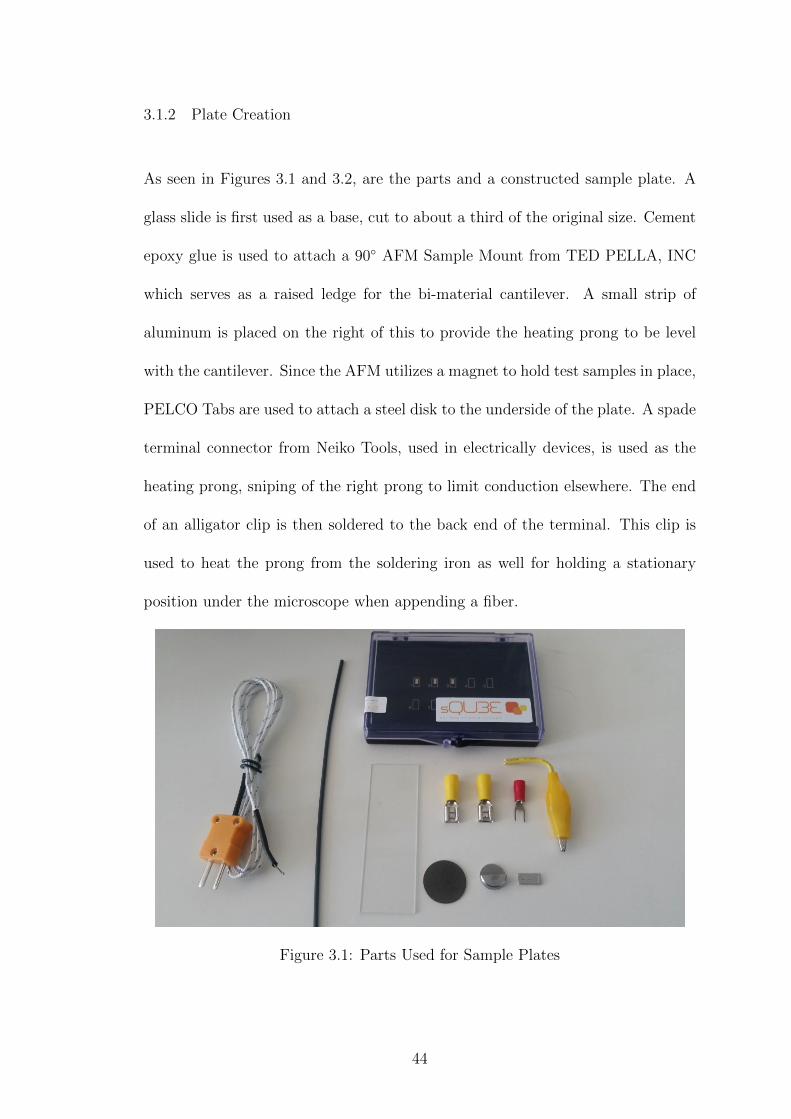
As seen in Figures 3.1 and 3.2, are the parts and a constructed sample plate. A
glass slide is first used as a base, cut to about a third of the original size. Cement
epoxy glue is used to attach a 90◦ AFM Sample Mount from TED PELLA, INC
which serves as a raised ledge for the bi-material cantilever. A small strip of
aluminum is placed on the right of this to provide the heating prong to be level
with the cantilever. Since the AFM utilizes a magnet to hold test samples in place,
PELCO Tabs are used to attach a steel disk to the underside of the plate. A spade
terminal connector from Neiko Tools, used in electrically devices, is used as the
heating prong, sniping of the right prong to limit conduction elsewhere. The end
of an alligator clip is then soldered to the back end of the terminal. This clip is
used to heat the prong from the soldering iron as well for holding a stationary
position under the microscope when appending a fiber.
Figure 3.1: Parts Used for Sample Plates
44
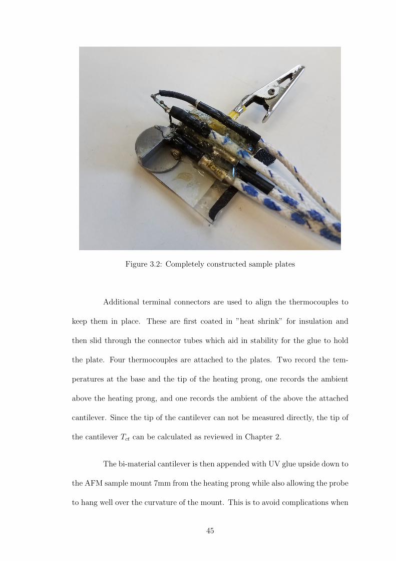
Figure 3.2: Completely constructed sample plates
Additional terminal connectors are used to align the thermocouples to
keep them in place. These are first coated in ”heat shrink” for insulation and
then slid through the connector tubes which aid in stability for the glue to hold
the plate. Four thermocouples are attached to the plates. Two record the tem-
peratures at the base and the tip of the heating prong, one records the ambient
above the heating prong, and one records the ambient of the above the attached
cantilever. Since the tip of the cantilever can not be measured directly, the tip of
the cantilever Tct can be calculated as reviewed in Chapter 2.
The bi-material cantilever is then appended with UV glue upside down to
the AFM sample mount 7mm from the heating prong while also allowing the probe
to hang well over the curvature of the mount. This is to avoid complications when
45
loading a fiber to the probe and AFM for measurements. To not potentially break
break a probe, the cantilever should be appended just before fiber appending.
3.2 Fiber Creation
As explained previously in section (1.1) morphology and fiber properties are key
in obtaining uniform thermally conductive nanofibers. The molecular chain length
and the molecular weight of a polymer is vital when choosing a ”good” solvent
to use [64, 65]. The first step for creating nanofibers is to properly formulate
a solution for different polymers needed for measurement. Depending on the
polymer being used for spinning, there are certain solvent carriers that work best
with the polymer. This is due to the ability of the solvent to fully dissolve the
polymer.
The polymer to be used for spinning and alternatively measuring the
thermal conductivity needs to be determined. There are many different polymers
to choose from depending on the use. Electrospun nanofibers can be useful in
such fields as electrical or even biomedical. In the biomedical field, these fiber
matrices have shown morphological similarities to natural extra-cellular matrices,
characterized by ultrafine continuous fibers, high surface-to-volume ratio, high
porosity and variable pore-size distributions [66]. Solution properties such as so-
lution viscosity, conductivity, dielectric constant, and surface tension may go into
the decision on a polymer needed.
In the proposed experiment, the chosen polymer is polycaprolactone
(PCL) with a density (px) of 1.145g/mL at room temperature and a melting
46
point of 60◦C. The reason for using polycaprolactone is due to the biomedical
usage. PCL is known as a synthetic biodegradable aliphatic polyester for uses in
tissue engineering, scaffolds, nerve guides, and drug delivery systems [67]. Since
acetone is the working solvent, PCL works best [68]. Additionally acetone is the
low end of the spectrum of toxicity, where solvents such as dimethylformamide
(DMF) or tetrahydrofuran (THF) have high ratings of such toxicity. Keep in
mind the melting point of PCL, this factors into the heating limit of the heating
prong and the fiber itself. There are additional solvent and polymer combinations
that produce more consistent and uniform fibers, that are more thermally con-
ductive and have a higher melting point. However, note that this is also not to
say that the method of creating a solution, the spinning process, or measuring
the thermal conductivity is any different. Further details of the produced fiber
properties can be seen in the Appendix.
With the chosen polymer we can move on to calculating a proper equation
to use for determining a useful weight of solute needed for the concentration. Using
a concentration of the polymer solution as w/v%, a sought after typical percentage
would be between 7.5% and 10% for this solution [68].
w
v% =
mass of the solute wx
volume of the solutionx 100 (3.1)
The optimization of electrospun fibers versus electrospraying is funda-
mental for electrospinnability. The determination of how the fibers are produced
depends a lot on the concentration of the solution itself. There is a certain minimal
concentration value that must be reached, which, if below this value, electrospray-
47
ing occurs or the formation of droplets only [69, 70]. This is because under high
voltage or electrical force the charge density of a droplets surface at the evaporation
point increases, the coulomb repulsion overcomes the surface tension and several
smaller droplets are formed. This is theorized by Rayleigh instability phenomena
[71, 72]. The higher the concentration the more stable the string of droplets be-
come [64]. On the other hand, if the concentration is too high and thus becomes
more viscous, uniform fibers will no longer be produced [73]. As the concentra-
tion of polymer increases, an overlapping of macromolecular chains occurs and
becomes important. The relative viscosity of solution increases significantly with
an increase in concentration, up to a critical concentration. This region, called
the semi-dilute regime, is found in the dimensionless concentration range of 1.0
to 10.0 [74, 75]. The Martin equation best describes the viscosity-concentration
relationship in concentrated polymer solutions [76, 74],
nsp
c[n]= eKmc[n] (3.2)
where nsp is the specific viscosity, c is the concentration of polymer so-
lution, [n] is the intrinsic viscosity of the polymer, and Km is a constant and it is
a measure of polymer-polymer and polymer-solvent interactions [74, 77].
Knowing what concentrations to use, next is to determine how much
solute is needed. As seen in equation 3.3 the weight (wx) of polymer in grams to
use can be found utilizing 3.1 and rewritten in a general form,
wx =vy
1P− 1
px
(3.3)
48
where vy is the volume of solvent being used and P is the fraction of the
concentration wanted.
In this experiment, 20mL of acetone and a 10% PCL concentration was
used providing 2.191g of solute at 1.145g/mL. To obtain a proper solution, acetone
and the PCL were heated to about 40◦C on a hot plate until dissolved. The boiling
point of acetone is 56◦C so 40◦C is enough to help dissolve the polymer. This took
about 40 minutes to dissolve. This was also taking into account a solvent volume
of 20mL.
The reason for creating such a higher volume than needed is that the
total volume of the solution is that similar to the volume of the solvent. Therefore
when obtaining a concentration to use, the weight of the solute to the volume of
the solution is small. This infers that if the polymer homogenizes in to the solvent
that only the volume of the solvent would have to be used. Moreover, in other
cases requiring a higher concentration or smaller solution volumes, the volume of
the solute or polymer should be taken into account. In this case, using PCL, the
acetone is poor at dissolving PCL properly, therefore the general form of equation
3.3 should be used. However in the case of using other polymers and solvents a
wt% should be used; this is because the solution will become homogeneous. Once
the solution is made the next step is to set up the solution for spinning.
3.3 Electrospinning Apparatus
For a traditional electrospinning apparatus only a few general items are needed, a
high voltage power supply up to 30kV, a syringe pump, electrode connected to a
49
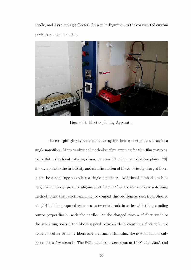
needle, and a grounding collector. As seen in Figure 3.3 is the constructed custom
electrospinning apparatus.
Figure 3.3: Electrospinning Apparatus
Electrospinnging systems can be setup for sheet collection as well as for a
single nanofiber. Many traditional methods utilize spinning for thin film matrices,
using flat, cylindrical rotating drum, or even 3D columnar collector plates [78].
However, due to the instability and chaotic motion of the electrically charged fibers
it can be a challenge to collect a single nanofiber. Additional methods such as
magnetic fields can produce alignment of fibers [79] or the utilization of a drawing
method, other than electrospinning, to combat this problem as seen from Shen et
al. (2010). The proposed system uses two steel rods in series with the grounding
source perpendicular with the needle. As the charged stream of fiber tends to
the grounding source, the fibers append between them creating a fiber web. To
avoid collecting to many fibers and creating a thin film, the system should only
be run for a few seconds. The PCL nanofibers were spun at 10kV with .3mA and
50
a working electrode distance of 9cm.
Using a chosen solution, the syringe is placed into the syringe pump.
Depending on the viscosity or concentration of the solution, a correct needle and
flow rate for spinning should be determined. With a flow rate applied, the fluid
should drip out at a consistent rate, as a drip flows out, a second drop should
replace it immediately. The smaller the needle, the lower the concentration should
be and vise-versa. In the case of using a 10% weight/volume solution of acetone
and PCL a needle gauge of 20AWG at a flow rate of 1 mL/min is recommended.
However, the applied voltage also needs to work in tandem with this flow rate.
The voltage applied depends on the distance of the needle to the collector. With
this, a critical voltage Vc can be expressed to determine the electric field needed
to develop fluid instability. Taylor (1964) also showed that this can be expressed
as:
V 2c = 4
H2
L2(ln
2L
R− 1.5)(0.117πRσ) (3.4)
where H is the distance between the needle tip and collector, L is the
length of the needle, R is the radius of the needle, and σ is the surface tension
of the liquid [30, 26, 80]. Equation 3.4 may be useful in determining a proper
applied voltage. A voltage around 10kV DC was found to be the workable amount
to spin PCL polymer nanofibers. Once the fibers are spun, they can be collected,
measured for dimensions, and appended to the sample plates.
51
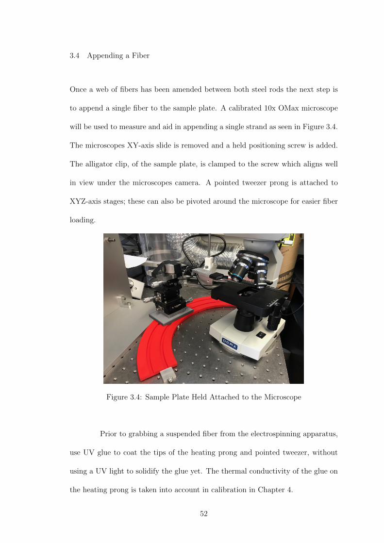
3.4 Appending a Fiber
Once a web of fibers has been amended between both steel rods the next step is
to append a single fiber to the sample plate. A calibrated 10x OMax microscope
will be used to measure and aid in appending a single strand as seen in Figure 3.4.
The microscopes XY-axis slide is removed and a held positioning screw is added.
The alligator clip, of the sample plate, is clamped to the screw which aligns well
in view under the microscopes camera. A pointed tweezer prong is attached to
XYZ-axis stages; these can also be pivoted around the microscope for easier fiber
loading.
Figure 3.4: Sample Plate Held Attached to the Microscope
Prior to grabbing a suspended fiber from the electrospinning apparatus,
use UV glue to coat the tips of the heating prong and pointed tweezer, without
using a UV light to solidify the glue yet. The thermal conductivity of the glue on
the heating prong is taken into account in calibration in Chapter 4.
52
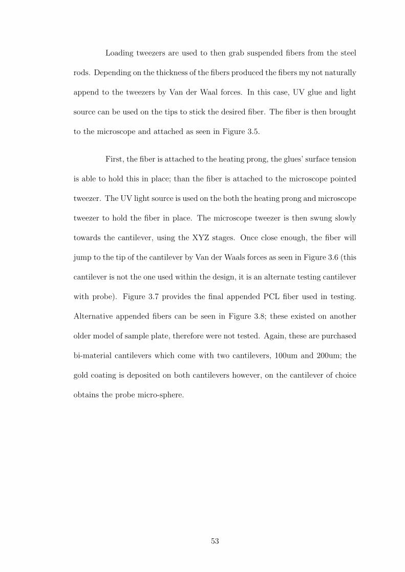
Loading tweezers are used to then grab suspended fibers from the steel
rods. Depending on the thickness of the fibers produced the fibers my not naturally
append to the tweezers by Van der Waal forces. In this case, UV glue and light
source can be used on the tips to stick the desired fiber. The fiber is then brought
to the microscope and attached as seen in Figure 3.5.
First, the fiber is attached to the heating prong, the glues’ surface tension
is able to hold this in place; than the fiber is attached to the microscope pointed
tweezer. The UV light source is used on the both the heating prong and microscope
tweezer to hold the fiber in place. The microscope tweezer is then swung slowly
towards the cantilever, using the XYZ stages. Once close enough, the fiber will
jump to the tip of the cantilever by Van der Waals forces as seen in Figure 3.6 (this
cantilever is not the one used within the design, it is an alternate testing cantilever
with probe). Figure 3.7 provides the final appended PCL fiber used in testing.
Alternative appended fibers can be seen in Figure 3.8; these existed on another
older model of sample plate, therefore were not tested. Again, these are purchased
bi-material cantilevers which come with two cantilevers, 100um and 200um; the
gold coating is deposited on both cantilevers however, on the cantilever of choice
obtains the probe micro-sphere.
53
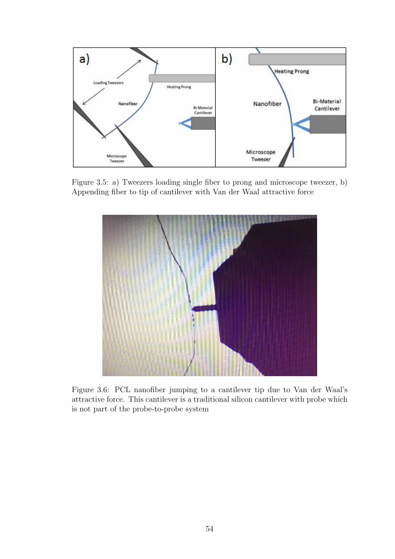
Figure 3.5: a) Tweezers loading single fiber to prong and microscope tweezer, b)Appending fiber to tip of cantilever with Van der Waal attractive force
Figure 3.6: PCL nanofiber jumping to a cantilever tip due to Van der Waal’sattractive force. This cantilever is a traditional silicon cantilever with probe whichis not part of the probe-to-probe system
54
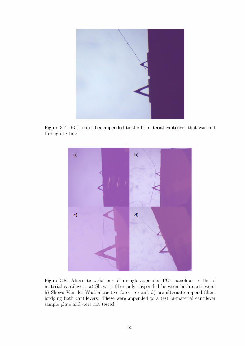
Figure 3.7: PCL nanofiber appended to the bi-material cantilever that was putthrough testing
Figure 3.8: Alternate variations of a single appended PCL nanofiber to the bimaterial cantilever. a) Shows a fiber only suspended between both cantilevers.b) Shows Van der Waal attractive force. c) and d) are alternate append fibersbridging both cantilevers. These were appended to a test bi-material cantileversample plate and were not tested.
55
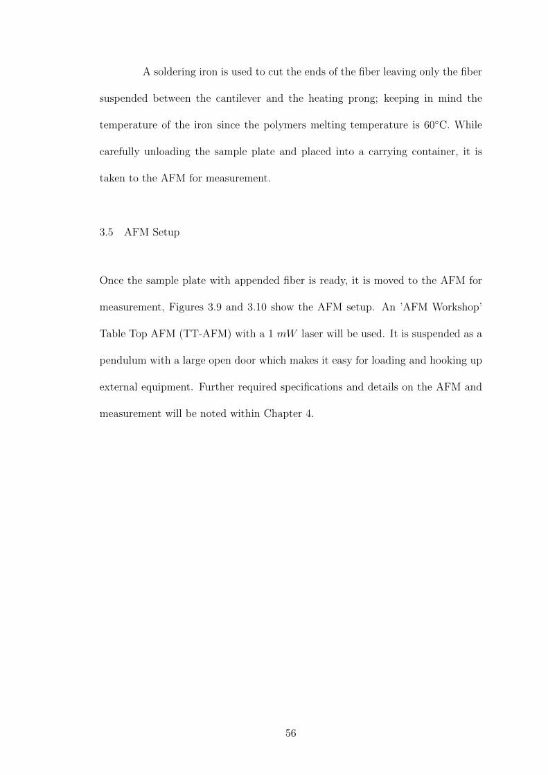
A soldering iron is used to cut the ends of the fiber leaving only the fiber
suspended between the cantilever and the heating prong; keeping in mind the
temperature of the iron since the polymers melting temperature is 60◦C. While
carefully unloading the sample plate and placed into a carrying container, it is
taken to the AFM for measurement.
3.5 AFM Setup
Once the sample plate with appended fiber is ready, it is moved to the AFM for
measurement, Figures 3.9 and 3.10 show the AFM setup. An ’AFM Workshop’
Table Top AFM (TT-AFM) with a 1 mW laser will be used. It is suspended as a
pendulum with a large open door which makes it easy for loading and hooking up
external equipment. Further required specifications and details on the AFM and
measurement will be noted within Chapter 4.
56
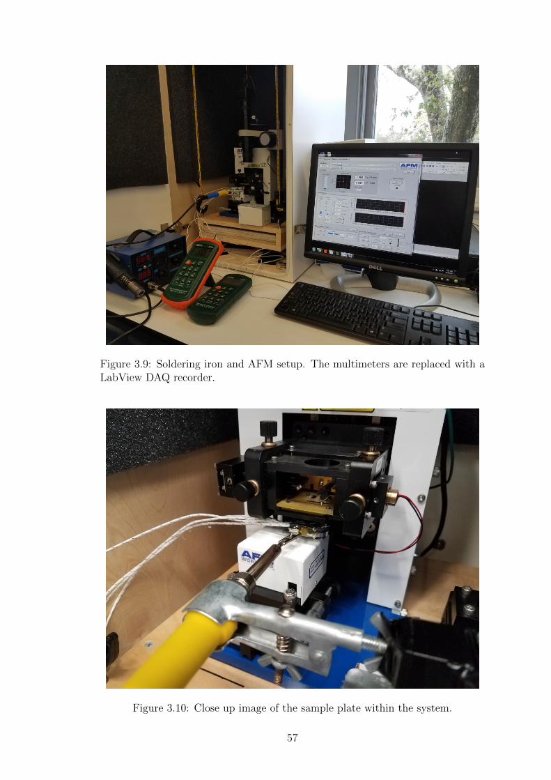
Figure 3.9: Soldering iron and AFM setup. The multimeters are replaced with aLabView DAQ recorder.
Figure 3.10: Close up image of the sample plate within the system.
57
A tipless silicon cantilever is loaded into the AFM as for typical use, this
is the AFM-tipless cantilever. The sample plate is then slid onto the stage with
the alligator clip facing out underneath the AFM cantilever. During measurement,
the cantilevers should line up as seen back in Figure 1.5. This alignment will be
seen further in Chapter 4. A simple stand and clamp is used to hold the soldering
iron. This should be brought to level with the sample plate, and fixed to the
alligator clip seen in Figure 3.10. The stand is on the pendulum platform due
to consistent swaying from camera and laser re-positioning and alignments; this
eliminates the sample plate from shifting out of position. The sample plates’ four
thermocouples are then plugged into a LabView DAQ system. The chamber door
is then closed to limit air flow. The AFM is now setup for testing.
58
Chapter 4
Methodology and Calibration
This chapter reviews the system settings and parameters used, along with how
to conduct and measure the thermal conductivity of electrospun nanofibers. Be-
fore any measurements are to be recorded, the AFM cantilevers responses and
settings will first need to be understood. The resonance frequency will initially
be measured, to validate that its force constant is indeed lower than that of the
bi-material cantilever. Once this is proven, the cantilever will be tested in contact
with bi-material cantilevers silicon base to show baseline changes in nm/C values,
seen in Chapter 5. This will first, show how the AFM cantilever will react un-
der varied temperatures without the bi-material cantilever and secondly, indicate
proper PID settings needed.
After the AFM cantilever parameters and settings have been determined,
the Probe-to-Probe system will then be set up to determine the calibrated temper-
ature vs deflection recordings; results of these recordings can be seen in Chapter
5.
59
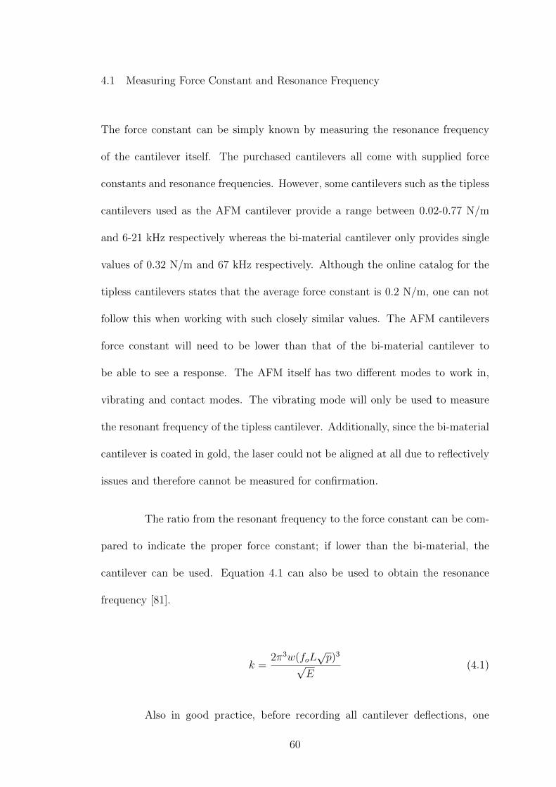
4.1 Measuring Force Constant and Resonance Frequency
The force constant can be simply known by measuring the resonance frequency
of the cantilever itself. The purchased cantilevers all come with supplied force
constants and resonance frequencies. However, some cantilevers such as the tipless
cantilevers used as the AFM cantilever provide a range between 0.02-0.77 N/m
and 6-21 kHz respectively whereas the bi-material cantilever only provides single
values of 0.32 N/m and 67 kHz respectively. Although the online catalog for the
tipless cantilevers states that the average force constant is 0.2 N/m, one can not
follow this when working with such closely similar values. The AFM cantilevers
force constant will need to be lower than that of the bi-material cantilever to
be able to see a response. The AFM itself has two different modes to work in,
vibrating and contact modes. The vibrating mode will only be used to measure
the resonant frequency of the tipless cantilever. Additionally, since the bi-material
cantilever is coated in gold, the laser could not be aligned at all due to reflectively
issues and therefore cannot be measured for confirmation.
The ratio from the resonant frequency to the force constant can be com-
pared to indicate the proper force constant; if lower than the bi-material, the
cantilever can be used. Equation 4.1 can also be used to obtain the resonance
frequency [81].
k =2π3w(foL
√p)3
√E
(4.1)
Also in good practice, before recording all cantilever deflections, one
60
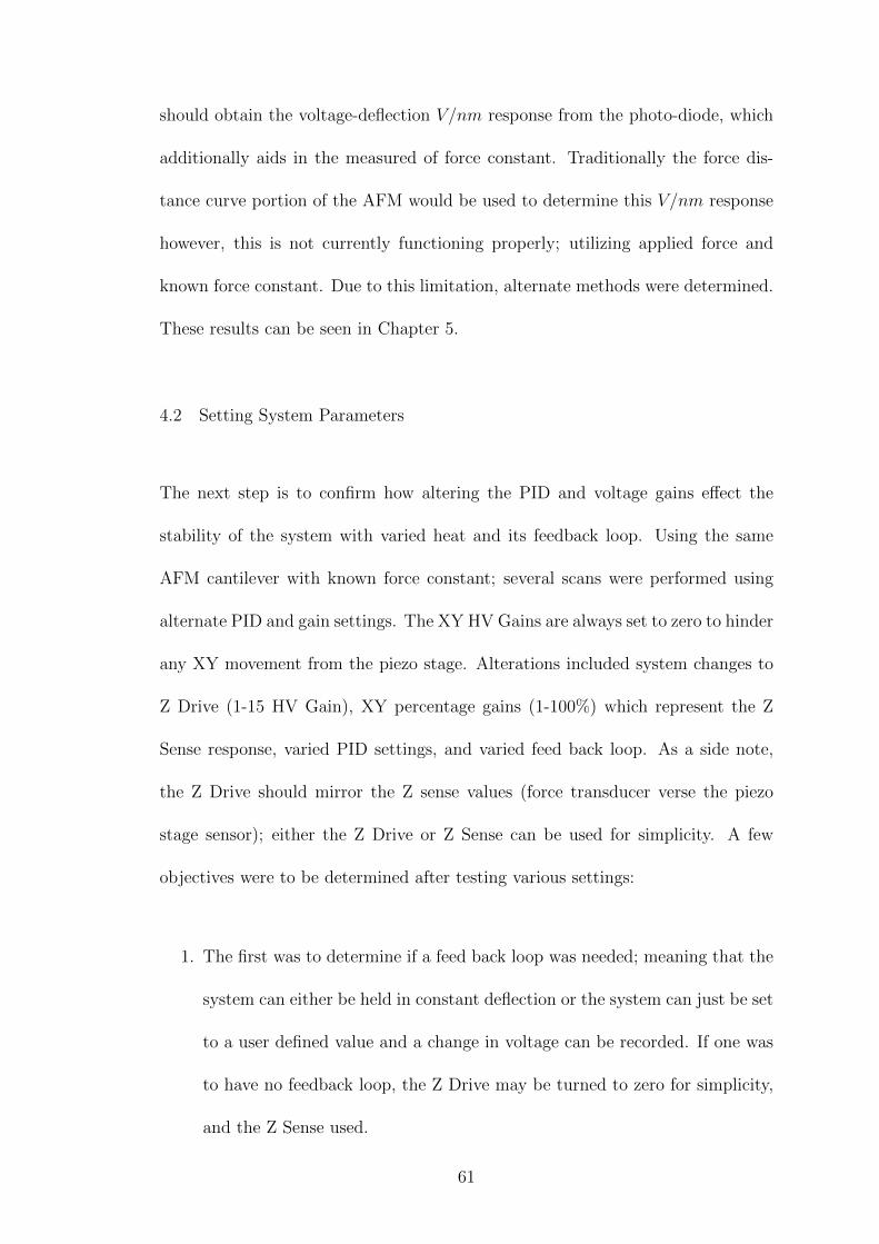
should obtain the voltage-deflection V/nm response from the photo-diode, which
additionally aids in the measured of force constant. Traditionally the force dis-
tance curve portion of the AFM would be used to determine this V/nm response
however, this is not currently functioning properly; utilizing applied force and
known force constant. Due to this limitation, alternate methods were determined.
These results can be seen in Chapter 5.
4.2 Setting System Parameters
The next step is to confirm how altering the PID and voltage gains effect the
stability of the system with varied heat and its feedback loop. Using the same
AFM cantilever with known force constant; several scans were performed using
alternate PID and gain settings. The XY HV Gains are always set to zero to hinder
any XY movement from the piezo stage. Alterations included system changes to
Z Drive (1-15 HV Gain), XY percentage gains (1-100%) which represent the Z
Sense response, varied PID settings, and varied feed back loop. As a side note,
the Z Drive should mirror the Z sense values (force transducer verse the piezo
stage sensor); either the Z Drive or Z Sense can be used for simplicity. A few
objectives were to be determined after testing various settings:
1. The first was to determine if a feed back loop was needed; meaning that the
system can either be held in constant deflection or the system can just be set
to a user defined value and a change in voltage can be recorded. If one was
to have no feedback loop, the Z Drive may be turned to zero for simplicity,
and the Z Sense used.
61
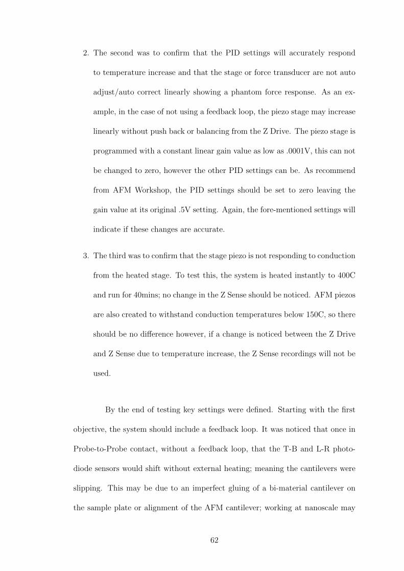
2. The second was to confirm that the PID settings will accurately respond
to temperature increase and that the stage or force transducer are not auto
adjust/auto correct linearly showing a phantom force response. As an ex-
ample, in the case of not using a feedback loop, the piezo stage may increase
linearly without push back or balancing from the Z Drive. The piezo stage is
programmed with a constant linear gain value as low as .0001V, this can not
be changed to zero, however the other PID settings can be. As recommend
from AFM Workshop, the PID settings should be set to zero leaving the
gain value at its original .5V setting. Again, the fore-mentioned settings will
indicate if these changes are accurate.
3. The third was to confirm that the stage piezo is not responding to conduction
from the heated stage. To test this, the system is heated instantly to 400C
and run for 40mins; no change in the Z Sense should be noticed. AFM piezos
are also created to withstand conduction temperatures below 150C, so there
should be no difference however, if a change is noticed between the Z Drive
and Z Sense due to temperature increase, the Z Sense recordings will not be
used.
By the end of testing key settings were defined. Starting with the first
objective, the system should include a feedback loop. It was noticed that once in
Probe-to-Probe contact, without a feedback loop, that the T-B and L-R photo-
diode sensors would shift without external heating; meaning the cantilevers were
slipping. This may be due to an imperfect gluing of a bi-material cantilever on
the sample plate or alignment of the AFM cantilever; working at nanoscale may
62
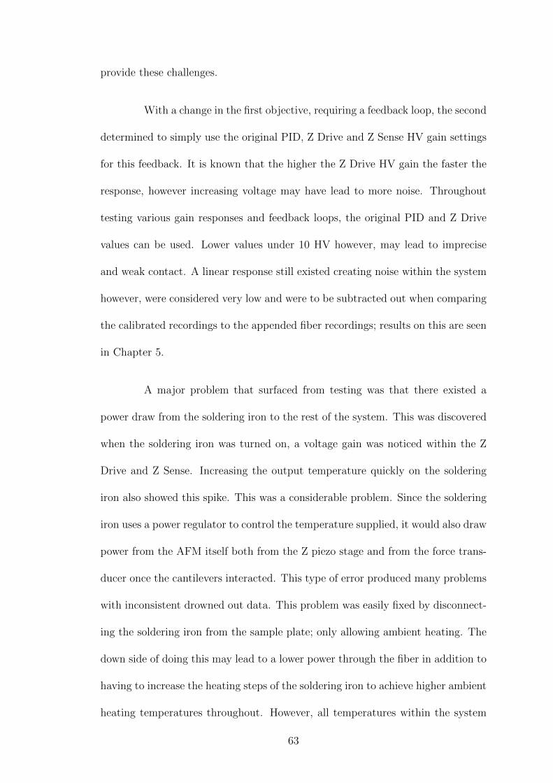
provide these challenges.
With a change in the first objective, requiring a feedback loop, the second
determined to simply use the original PID, Z Drive and Z Sense HV gain settings
for this feedback. It is known that the higher the Z Drive HV gain the faster the
response, however increasing voltage may have lead to more noise. Throughout
testing various gain responses and feedback loops, the original PID and Z Drive
values can be used. Lower values under 10 HV however, may lead to imprecise
and weak contact. A linear response still existed creating noise within the system
however, were considered very low and were to be subtracted out when comparing
the calibrated recordings to the appended fiber recordings; results on this are seen
in Chapter 5.
A major problem that surfaced from testing was that there existed a
power draw from the soldering iron to the rest of the system. This was discovered
when the soldering iron was turned on, a voltage gain was noticed within the Z
Drive and Z Sense. Increasing the output temperature quickly on the soldering
iron also showed this spike. This was a considerable problem. Since the soldering
iron uses a power regulator to control the temperature supplied, it would also draw
power from the AFM itself both from the Z piezo stage and from the force trans-
ducer once the cantilevers interacted. This type of error produced many problems
with inconsistent drowned out data. This problem was easily fixed by disconnect-
ing the soldering iron from the sample plate; only allowing ambient heating. The
down side of doing this may lead to a lower power through the fiber in addition to
having to increase the heating steps of the soldering iron to achieve higher ambient
heating temperatures throughout. However, all temperatures within the system
63
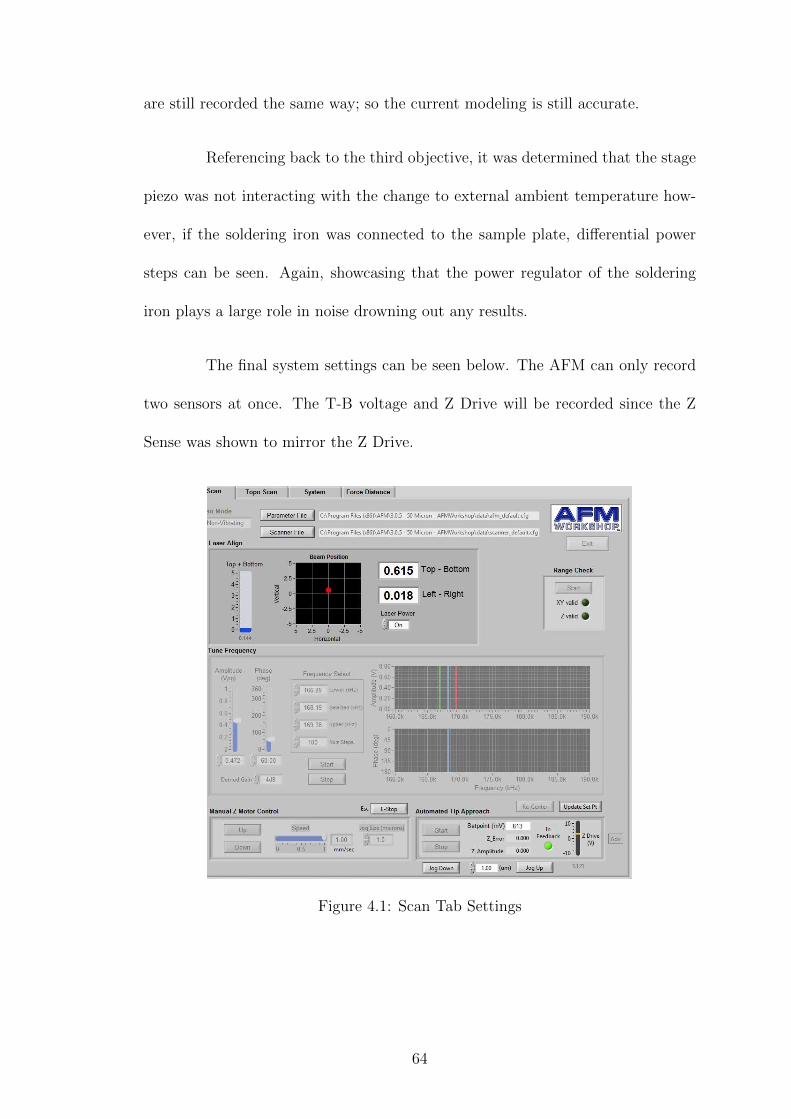
are still recorded the same way; so the current modeling is still accurate.
Referencing back to the third objective, it was determined that the stage
piezo was not interacting with the change to external ambient temperature how-
ever, if the soldering iron was connected to the sample plate, differential power
steps can be seen. Again, showcasing that the power regulator of the soldering
iron plays a large role in noise drowning out any results.
The final system settings can be seen below. The AFM can only record
two sensors at once. The T-B voltage and Z Drive will be recorded since the Z
Sense was shown to mirror the Z Drive.
Figure 4.1: Scan Tab Settings
64
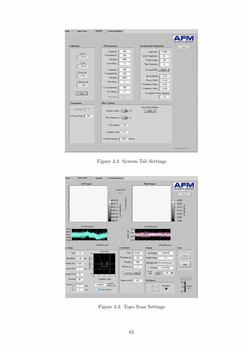
Figure 4.2: System Tab Settings
Figure 4.3: Topo Scan Settings
65
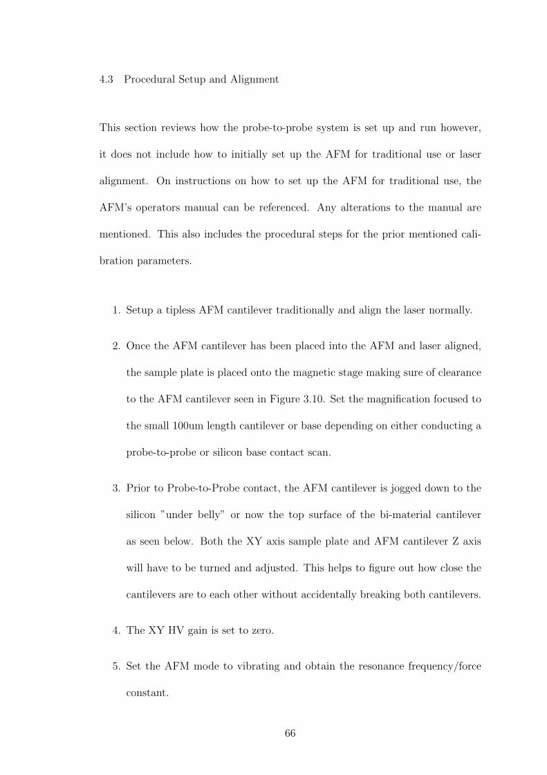
4.3 Procedural Setup and Alignment
This section reviews how the probe-to-probe system is set up and run however,
it does not include how to initially set up the AFM for traditional use or laser
alignment. On instructions on how to set up the AFM for traditional use, the
AFM’s operators manual can be referenced. Any alterations to the manual are
mentioned. This also includes the procedural steps for the prior mentioned cali-
bration parameters.
1. Setup a tipless AFM cantilever traditionally and align the laser normally.
2. Once the AFM cantilever has been placed into the AFM and laser aligned,
the sample plate is placed onto the magnetic stage making sure of clearance
to the AFM cantilever seen in Figure 3.10. Set the magnification focused to
the small 100um length cantilever or base depending on either conducting a
probe-to-probe or silicon base contact scan.
3. Prior to Probe-to-Probe contact, the AFM cantilever is jogged down to the
silicon ”under belly” or now the top surface of the bi-material cantilever
as seen below. Both the XY axis sample plate and AFM cantilever Z axis
will have to be turned and adjusted. This helps to figure out how close the
cantilevers are to each other without accidentally breaking both cantilevers.
4. The XY HV gain is set to zero.
5. Set the AFM mode to vibrating and obtain the resonance frequency/force
constant.
66
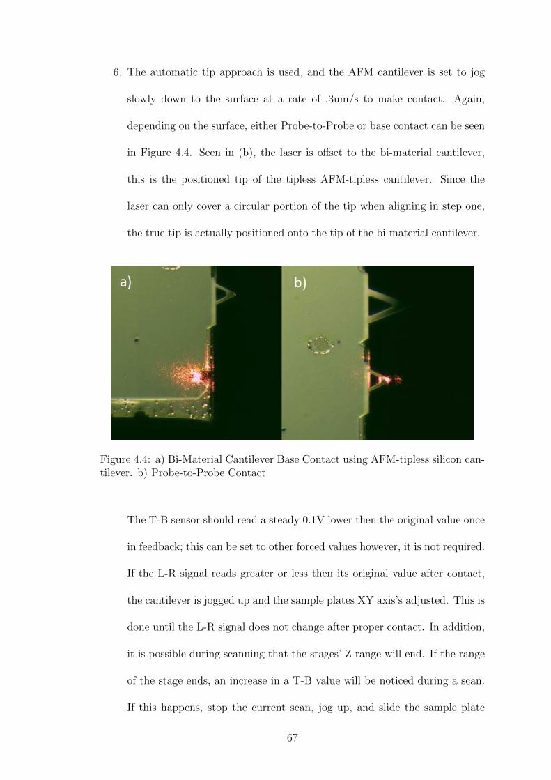
6. The automatic tip approach is used, and the AFM cantilever is set to jog
slowly down to the surface at a rate of .3um/s to make contact. Again,
depending on the surface, either Probe-to-Probe or base contact can be seen
in Figure 4.4. Seen in (b), the laser is offset to the bi-material cantilever,
this is the positioned tip of the tipless AFM-tipless cantilever. Since the
laser can only cover a circular portion of the tip when aligning in step one,
the true tip is actually positioned onto the tip of the bi-material cantilever.
Figure 4.4: a) Bi-Material Cantilever Base Contact using AFM-tipless silicon can-tilever. b) Probe-to-Probe Contact
The T-B sensor should read a steady 0.1V lower then the original value once
in feedback; this can be set to other forced values however, it is not required.
If the L-R signal reads greater or less then its original value after contact,
the cantilever is jogged up and the sample plates XY axis’s adjusted. This is
done until the L-R signal does not change after proper contact. In addition,
it is possible during scanning that the stages’ Z range will end. If the range
of the stage ends, an increase in a T-B value will be noticed during a scan.
If this happens, stop the current scan, jog up, and slide the sample plate
67
further centered on the magnetic stage. The entire scan will have to be
started over.
7. Once contact has been made, the Topo Scan tab will be used. The scan
rate is set to 0.42 Hz recording for about two 40 min scans, each containing
1024 scan lines; the AFM can only record so many scan lines within a given
time. Additionally, LabView is set up to record the thermocouples at a rate
of 0.42 Hz.
8. Then hit start on both devices. Once the number of scan lines reaches
increments of 256, the soldering iron is increased 50C. This gives about
10mins for each temperature increase to attain steady state.
9. Once each set of scans are complete, the LabView program is stopped; the
values are automatically saved off.
10. After both scans, the soldering iron is turned off and cooled for 20mins,
ready for another set of scans.
68
Chapter 5
Measurement Results and Discussion
This chapter compares all theoretical and measured results to determine the ther-
mal conductivity of the nanofibers. This also reviews recorded values for voltage
and natural deflection calibration results.
69
5.1 Introduction
There exist two different models to consider when obtaining measurements, the-
oretical and measured/recorded. Calibrated values and recordings are first con-
ducted in order to make sure recorded measurements match theoretical results.
The calibrated recordings of the Probe-to-Probe system without a fiber are com-
pared to the measured/recorded deflections with an appended fiber.
The theoretical values are obtained using the modeled functions from
Chapter 2, whereas the recorded values are sent to an Excel spreadsheet. Both the
theoretical and measured/recorded values are generated/called in to a MATLAB
program where depictions are shown. The theoretically calculated bi-material
cantilever temperatures Tct, where Tct is output temperature from the fiber to
the bi-material cantilever, will need to be theoretically generated since they can
not be measured. A difference in Tct should be noticed once a fiber is appended.
The temperature into the fiber from the heating prong, Tf , are also numerically
generated; the approximation for this is seen in Chapter 2 but the values are shown
further in this chapter. Once both Tct and Tf temperatures are known, the heat
conducted through the appended fiber kf will be known.
5.2 Deflection Results
The preceding recordings will showcase all measurements and theoretical results
of cantilever deflection with and without a fiber. Figure 5.1 shows the average
deflection with ambient temperature values reaching steady state after 8 minutes;
70
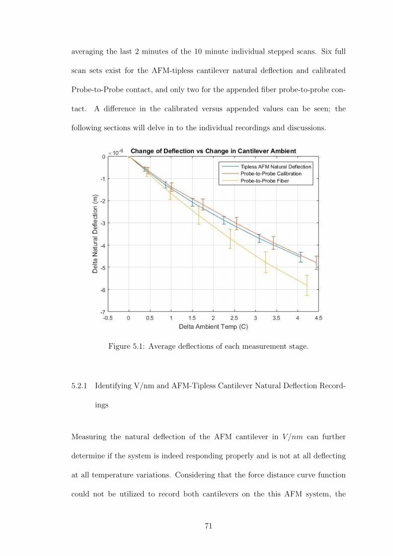
averaging the last 2 minutes of the 10 minute individual stepped scans. Six full
scan sets exist for the AFM-tipless cantilever natural deflection and calibrated
Probe-to-Probe contact, and only two for the appended fiber probe-to-probe con-
tact. A difference in the calibrated versus appended values can be seen; the
following sections will delve in to the individual recordings and discussions.
Figure 5.1: Average deflections of each measurement stage.
5.2.1 Identifying V/nm and AFM-Tipless Cantilever Natural Deflection Record-
ings
Measuring the natural deflection of the AFM cantilever in V/nm can further
determine if the system is indeed responding properly and is not at all deflecting
at all temperature variations. Considering that the force distance curve function
could not be utilized to record both cantilevers on the this AFM system, the
71
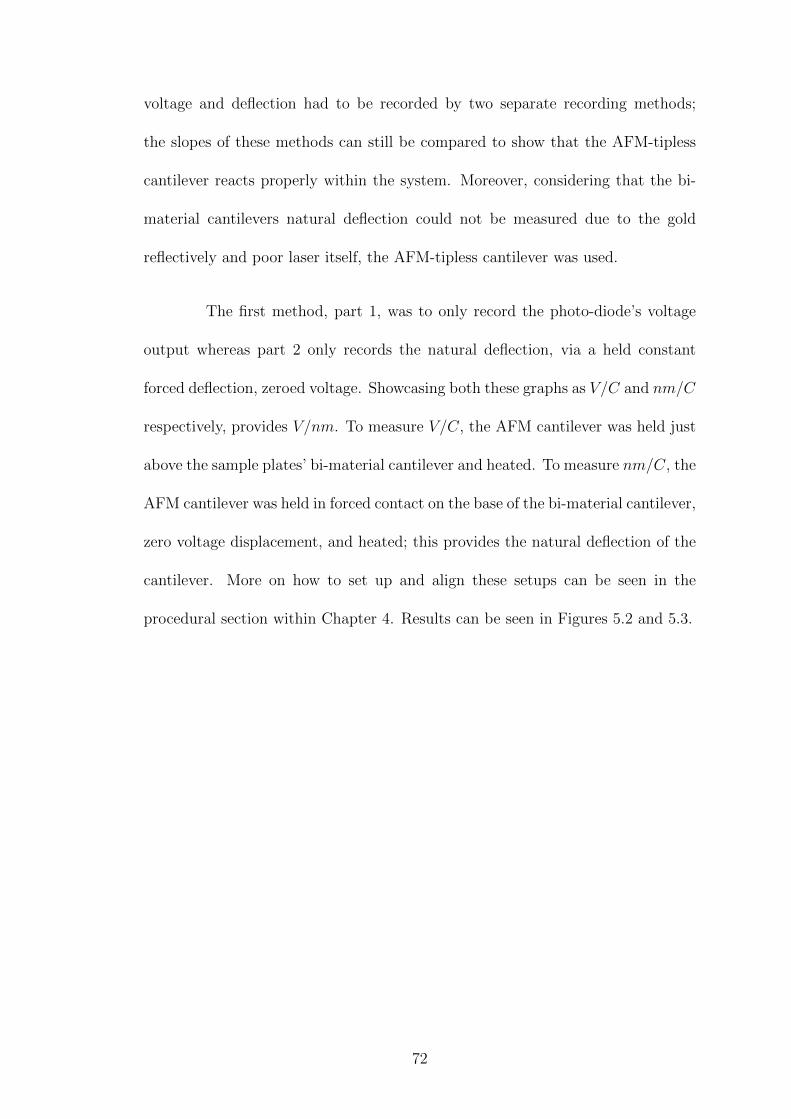
voltage and deflection had to be recorded by two separate recording methods;
the slopes of these methods can still be compared to show that the AFM-tipless
cantilever reacts properly within the system. Moreover, considering that the bi-
material cantilevers natural deflection could not be measured due to the gold
reflectively and poor laser itself, the AFM-tipless cantilever was used.
The first method, part 1, was to only record the photo-diode’s voltage
output whereas part 2 only records the natural deflection, via a held constant
forced deflection, zeroed voltage. Showcasing both these graphs as V/C and nm/C
respectively, provides V/nm. To measure V/C, the AFM cantilever was held just
above the sample plates’ bi-material cantilever and heated. To measure nm/C, the
AFM cantilever was held in forced contact on the base of the bi-material cantilever,
zero voltage displacement, and heated; this provides the natural deflection of the
cantilever. More on how to set up and align these setups can be seen in the
procedural section within Chapter 4. Results can be seen in Figures 5.2 and 5.3.
72
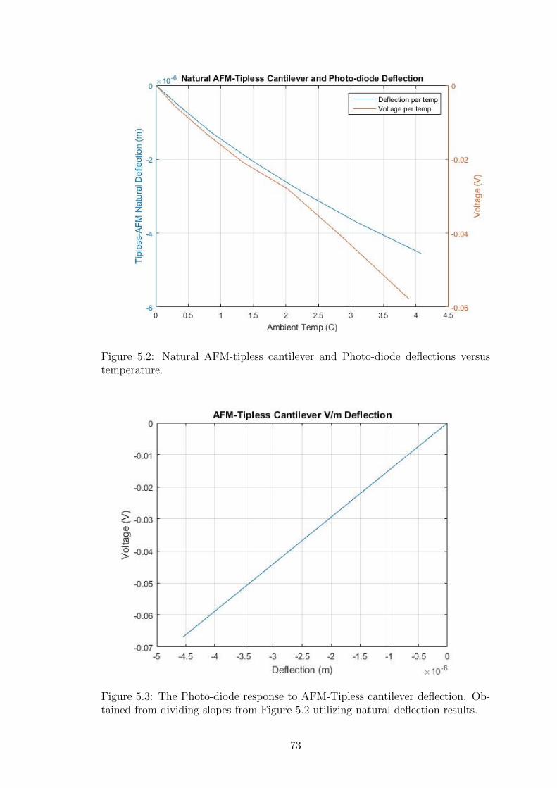
Figure 5.2: Natural AFM-tipless cantilever and Photo-diode deflections versustemperature.
Figure 5.3: The Photo-diode response to AFM-Tipless cantilever deflection. Ob-tained from dividing slopes from Figure 5.2 utilizing natural deflection results.
73
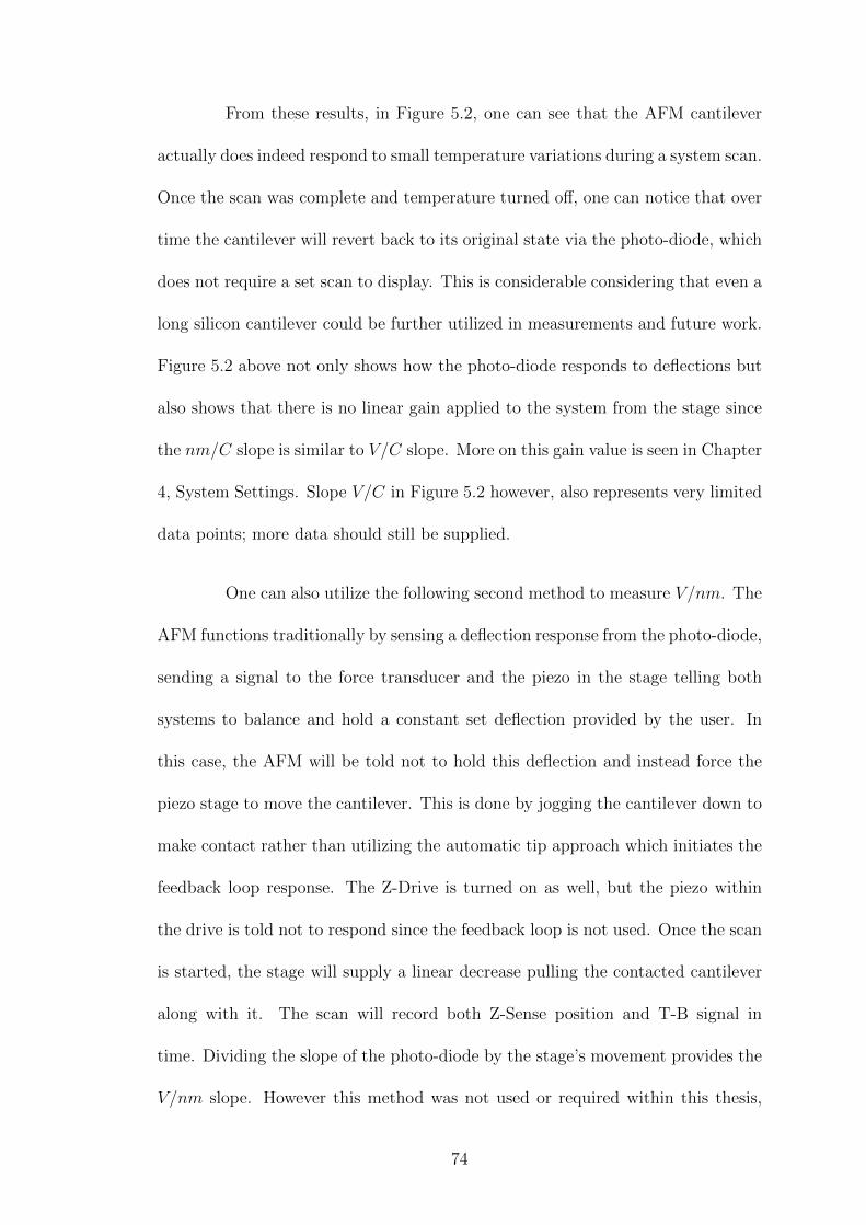
From these results, in Figure 5.2, one can see that the AFM cantilever
actually does indeed respond to small temperature variations during a system scan.
Once the scan was complete and temperature turned off, one can notice that over
time the cantilever will revert back to its original state via the photo-diode, which
does not require a set scan to display. This is considerable considering that even a
long silicon cantilever could be further utilized in measurements and future work.
Figure 5.2 above not only shows how the photo-diode responds to deflections but
also shows that there is no linear gain applied to the system from the stage since
the nm/C slope is similar to V/C slope. More on this gain value is seen in Chapter
4, System Settings. Slope V/C in Figure 5.2 however, also represents very limited
data points; more data should still be supplied.
One can also utilize the following second method to measure V/nm. The
AFM functions traditionally by sensing a deflection response from the photo-diode,
sending a signal to the force transducer and the piezo in the stage telling both
systems to balance and hold a constant set deflection provided by the user. In
this case, the AFM will be told not to hold this deflection and instead force the
piezo stage to move the cantilever. This is done by jogging the cantilever down to
make contact rather than utilizing the automatic tip approach which initiates the
feedback loop response. The Z-Drive is turned on as well, but the piezo within
the drive is told not to respond since the feedback loop is not used. Once the scan
is started, the stage will supply a linear decrease pulling the contacted cantilever
along with it. The scan will record both Z-Sense position and T-B signal in
time. Dividing the slope of the photo-diode by the stage’s movement provides the
V/nm slope. However this method was not used or required within this thesis,
74
the procedure can still applied to future works.
Figure 5.4 below shows how the AFM-tipless cantilever itself responded
to temperature variations when compared to its theoretical values. From the dis-
played results of V/C, from Figure 5.2, one can clearly notice change in deflection.
Figure 5.4: Theoretical versus Measured AFM-Tipless cantilever deflections.
There are no statements from the purchased cantilever manufacturer that
the silicon cantilever should respond to higher than normal variations in temper-
ature, only that they should not deflect in regular ambient room temperature.
Traditional uses of AFM do not include increases to ambient normally, so scans
would typically ignore this since ambient usually does not change. The system was
also tested by removing the AFM cantilever, then heating the system; no change
in the photo-diode was noticed. However, the actual theoretical result does match
expected results seen from Chapter 1, showing silicon cantilever temperature res-
75
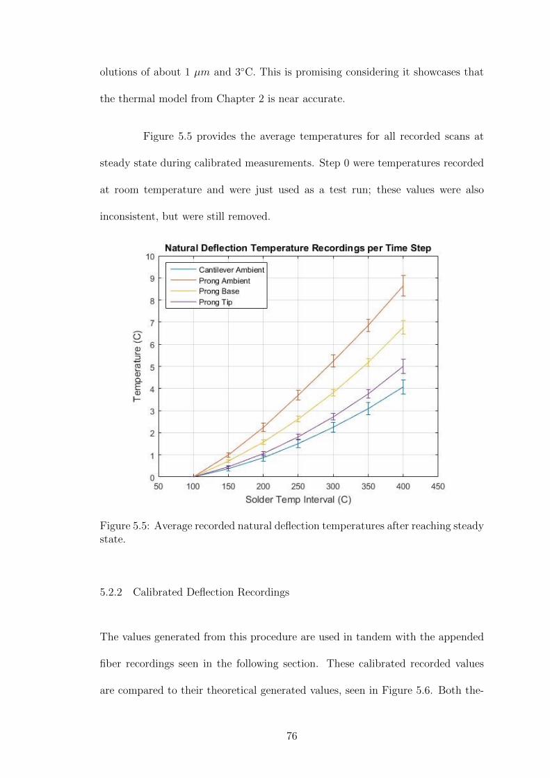
olutions of about 1 µm and 3◦C. This is promising considering it showcases that
the thermal model from Chapter 2 is near accurate.
Figure 5.5 provides the average temperatures for all recorded scans at
steady state during calibrated measurements. Step 0 were temperatures recorded
at room temperature and were just used as a test run; these values were also
inconsistent, but were still removed.
Figure 5.5: Average recorded natural deflection temperatures after reaching steadystate.
5.2.2 Calibrated Deflection Recordings
The values generated from this procedure are used in tandem with the appended
fiber recordings seen in the following section. These calibrated recorded values
are compared to their theoretical generated values, seen in Figure 5.6. Both the-
76
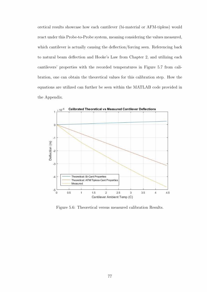
oretical results showcase how each cantilever (bi-material or AFM-tipless) would
react under this Probe-to-Probe system, meaning considering the values measured,
which cantilever is actually causing the deflection/forcing seen. Referencing back
to natural beam deflection and Hooke’s Law from Chapter 2, and utilizing each
cantilevers’ properties with the recorded temperatures in Figure 5.7 from cali-
bration, one can obtain the theoretical values for this calibration step. How the
equations are utilized can further be seen within the MATLAB code provided in
the Appendix.
Figure 5.6: Theoretical versus measured calibration Results.
77
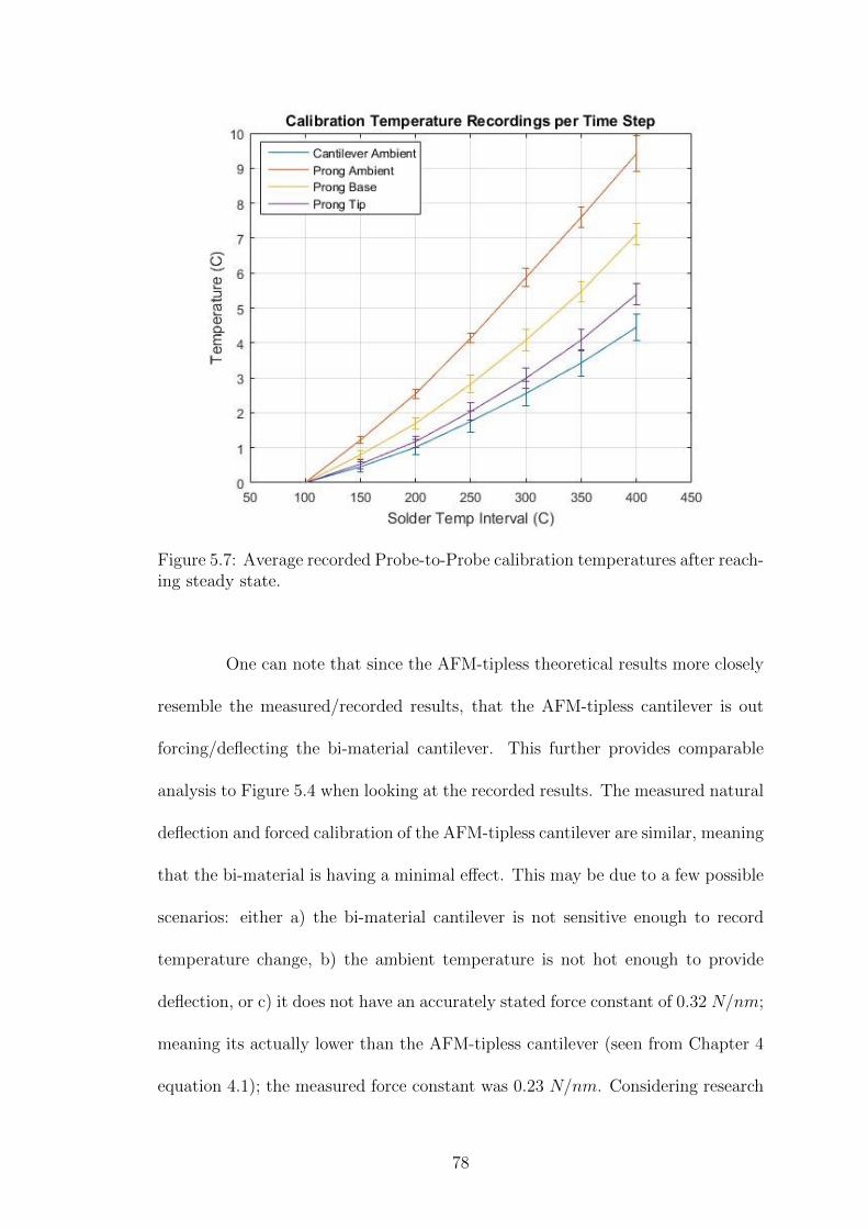
Figure 5.7: Average recorded Probe-to-Probe calibration temperatures after reach-ing steady state.
One can note that since the AFM-tipless theoretical results more closely
resemble the measured/recorded results, that the AFM-tipless cantilever is out
forcing/deflecting the bi-material cantilever. This further provides comparable
analysis to Figure 5.4 when looking at the recorded results. The measured natural
deflection and forced calibration of the AFM-tipless cantilever are similar, meaning
that the bi-material is having a minimal effect. This may be due to a few possible
scenarios: either a) the bi-material cantilever is not sensitive enough to record
temperature change, b) the ambient temperature is not hot enough to provide
deflection, or c) it does not have an accurately stated force constant of 0.32 N/nm;
meaning its actually lower than the AFM-tipless cantilever (seen from Chapter 4
equation 4.1); the measured force constant was 0.23 N/nm. Considering research
78
conducted on the sensitively of bi-material cantilevers, seen from Chapter 1, the
former should not be the case.
5.2.3 Appended Fiber Deflection Recordings
After recording deflection and temperature values once a fiber was appended, the
recorded slope must be subtracted from the recorded calibrated slope; this zeros
out data to provide a true deflection verses change in ambient temperature solution
seen in Figure 5.8. These new deflections are used within the MATLAB program
to supply the Tf and Tct values required; again, the theoretical values utilize
equations 2.22 and 2.69 respectively, assuming Tf = TfCal. In this experiment,
when the fiber was appended to the sample plate, the prong end of the fiber
was connected directly to the prong tip; this makes the assumption negated and
Tf = TfCal = Tpt and qf = qp1 provide equation simplification. Figure 5.9 provides
the averaged recorded temperatures.
79
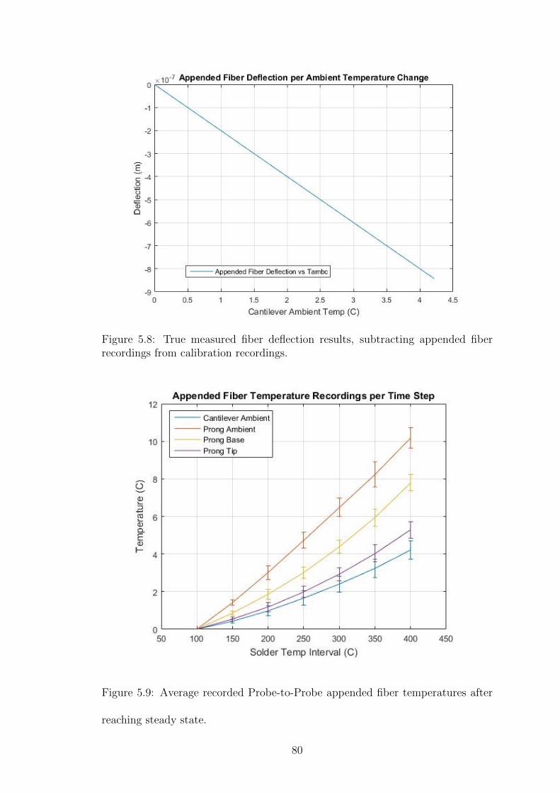
Figure 5.8: True measured fiber deflection results, subtracting appended fiberrecordings from calibration recordings.
Figure 5.9: Average recorded Probe-to-Probe appended fiber temperatures after
reaching steady state.
80
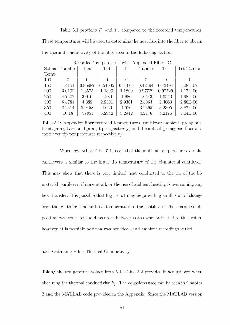
Table 5.1 provides Tf and Tct compared to the recorded temperatures.
These temperatures will be used to determine the heat flux into the fiber to obtain
the thermal conductivity of the fiber seen in the following section.
Recorded Temperatures with Appended Fiber ◦CSolderTemp
Tambp Tpo Tpt Tf Tambc Tct Tct-Tambc
100 0 0 0 0 0 0 0150 1.4151 0.85987 0.54005 0.54005 0.42494 0.42494 5.08E-07200 3.0192 1.8575 1.1809 1.1809 0.97729 0.97729 1.17E-06250 4.7307 3.016 1.986 1.986 1.6543 1.6543 1.98E-06300 6.4784 4.389 2.9301 2.9301 2.4063 2.4063 2.88E-06350 8.2314 5.9458 4.026 4.026 3.2395 3.2395 3.87E-06400 10.18 7.7851 5.2942 5.2942 4.2176 4.2176 5.04E-06
Table 5.1: Appended fiber recorded temperatures (cantilever ambient, prong am-bient, prong base, and prong tip respectively) and theoretical (prong end fiber andcantilever tip temperatures respectively).
When reviewing Table 5.1, note that the ambient temperature over the
cantilevers is similar to the input tip temperature of the bi-material cantilever.
This may show that there is very limited heat conducted to the tip of the bi-
material cantilever, if none at all, or the use of ambient heating is overcoming any
heat transfer. It is possible that Figure 5.1 may be providing an illusion of change
even though there is no additive temperature to the cantilever. The thermocouple
position was consistent and accurate between scans when adjusted to the system
however, it is possible position was not ideal, and ambient recordings varied.
5.3 Obtaining Fiber Thermal Conductivity
Taking the temperature values from 5.1, Table 5.2 provides fluxes utilized when
obtaining the thermal conductivity kf . The equations used can be seen in Chapter
2 and the MATLAB code provided in the Appendix. Since the MATLAB version
81
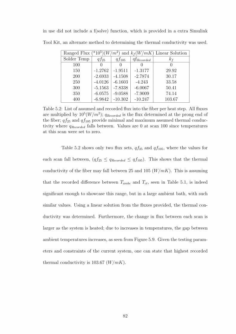
in use did not include a f(solve) function, which is provided in a extra Simulink
Tool Kit, an alternate method to determining the thermal conductivity was used.
Ranged Flux (*105)(W/m2) and kf (W/mK) Linear SolutionSolder Temp qf25 qf105 qfRecorded kf
100 0 0 0 0150 -1.2762 -1.9511 -1.3177 29.92200 -2.6933 -4.1508 -2.7874 30.17250 -4.0126 -6.1603 -4.243 33.58300 -5.1563 -7.8338 -6.0067 50.41350 -6.0575 -9.0588 -7.9009 74.14400 -6.9842 -10.302 -10.247 103.67
Table 5.2: List of assumed and recorded flux into the fiber per heat step. All fluxesare multiplied by 105(W/m2); qRecorded is the flux determined at the prong end ofthe fiber; qf25 and qf105 provide minimal and maximum assumed thermal conduc-tivity where qRecorded falls between. Values are 0 at scan 100 since temperaturesat this scan were set to zero.
Table 5.2 shows only two flux sets, qf25 and qf105, where the values for
each scan fall between, (qf25 ≤ qRecorded ≤ qf105). This shows that the thermal
conductivity of the fiber may fall between 25 and 105 (W/mK). This is assuming
that the recorded difference between Tambc and Tct, seen in Table 5.1, is indeed
significant enough to showcase this range, but in a large ambient bath, with such
similar values. Using a linear solution from the fluxes provided, the thermal con-
ductivity was determined. Furthermore, the change in flux between each scan is
larger as the system is heated; due to increases in temperatures, the gap between
ambient temperatures increases, as seen from Figure 5.9. Given the testing param-
eters and constraints of the current system, one can state that highest recorded
thermal conductivity is 103.67 (W/mK).
82
Chapter 6
Summary and Future Work
The chapter details end thesis conclusions and takeaways along with design ideas
that can be incorporated in future works.
83

6.1 Chapter Summaries
This section reviews each chapter, the resulting conclusions and details noticed.
Chapter 1 - Provided background information on nanoscale thermal trans-
port, past measurement techniques, and defined the proposed Probe-to-Probe de-
sign.
Chapter 2 - Defined introductory heat transfer along with the detailed
modeled design of the Probe-to-Probe system. It further provided listed equations
to obtain unknowns such as system and fiber fluxes, system cantilever and prong
temperatures, and forced and natural deflections, all of which required to solve for
the thermal conductivity of an appended nanofiber.
Chapter 3 - Focused on the experimental apparatus, fiber and sample
plate creation, and equipment used. System properties such as bi-material can-
tilever, AFM-tipless cantilever, and electrospun PCL nanofibers were obtained,
which are further seen in the Appendix.
Chapter 4 - Reviewed the procedural measurement of the system and
outlined how the system was calibrated, along with how each system setting were
determined. It was found that the bi-material cantilevers’ natural deflection to
ambient changes could not be measured due to inert reflectively possibly due to
the strength and focus of the laser. A voltage draw was also noticed when in a
conductive heat transfer system. This was fixed by disconnecting the soldering
iron from the sample plate and recording all temperatures as normal.
84
Chapter 5 - Detailed all the results from testing including: natural de-
flections, pre-appended fiber calibrations, and appended fiber recordings. Each
section reviewed findings and comparisons of measured results to theoretical ex-
pectations, along with explanations and conclusions. Minimal deflection was seen
from the bi-material cantilever due to unexpected deflections from AFM-tipless
cantilever. Results matching this seen deflection do not coincide with theoretical
results. However, theoretical silicon cantilever natural deflection results match
expected results seen from Chapter 1 showing silicon cantilever temperature res-
olutions of about 1 µm and 3◦C. This was promising considering it showcases
that the thermal model from Chapter 2 is near accurate; measured results do not
match.
Furthermore, thermal conductivity values were determined to be between
25 and 105 (W/m2) when comparing flux. Following, given the testing parameters
and constraints of the current system, one can state that highest recorded thermal
conductance is 103.67 (W/m2). This was assuming that the extra temperature
at Tct is indeed significant enough to showcase this range, but in a large ambient
bath, with such similar values.
6.2 Future Work
A lot can be done to modify the Probe-to-Probe design; the first thing to consider
is the AFM itself. The AFM is still a very useful tool in measuring nanoscale
technology, however, the particular AFM model utilized within this thesis was
a simple model. There exists AFMs that can implement a Scanning Thermal
85
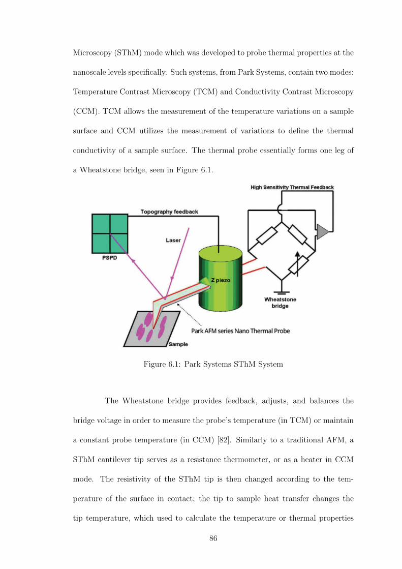
Microscopy (SThM) mode which was developed to probe thermal properties at the
nanoscale levels specifically. Such systems, from Park Systems, contain two modes:
Temperature Contrast Microscopy (TCM) and Conductivity Contrast Microscopy
(CCM). TCM allows the measurement of the temperature variations on a sample
surface and CCM utilizes the measurement of variations to define the thermal
conductivity of a sample surface. The thermal probe essentially forms one leg of
a Wheatstone bridge, seen in Figure 6.1.
Figure 6.1: Park Systems SThM System
The Wheatstone bridge provides feedback, adjusts, and balances the
bridge voltage in order to measure the probe’s temperature (in TCM) or maintain
a constant probe temperature (in CCM) [82]. Similarly to a traditional AFM, a
SThM cantilever tip serves as a resistance thermometer, or as a heater in CCM
mode. The resistivity of the SThM tip is then changed according to the tem-
perature of the surface in contact; the tip to sample heat transfer changes the
tip temperature, which used to calculate the temperature or thermal properties
86
of the sample at contact [83]. This would be very useful when determining the
thermal conductivity of a nanofiber rather than a planar surface. This may be
a promising technique when used in tandem with a vacuum. Kim et al. have
utilized an Ultra-High Vacuum (UHV)-based SThM technique that was capable
of quantitatively mapping temperature fields with about 15 mK temperature res-
olution and 10 nm spatial resolution [84]. However, the thermal transport around
the nanoscale contact area between a SThM probe tip and sample is still an issue
in SThM [85].
The second option would be to mitigate all ambient temperature utiliz-
ing a vacuum with with the current system or an SThM. Again, this would limit
thermal noise and excess heat into the system to provide only conductive heat
transfer. Considering the issue seen in Chapter 4 with voltage draw, this calibra-
tion would have been more easily noticed if the system was not in an ambient bath
skewing data.
The third would be to utilize alternate silicon or bi-material cantilevers.
This thesis utilized tipless silicon cantilevers however, there do exist lower con-
sistent force constant cantilevers that include probes. The rationale for placing
the probe on the bi-material cantilever instead was due to the purchasing ability;
these could not be purchased tipless.
87
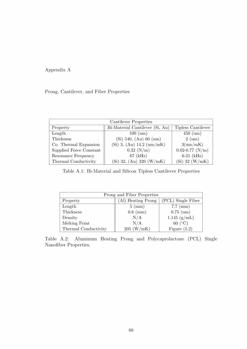
Appendix A
Prong, Cantilever, and Fiber Properties
Cantilever Properties
Property Bi-Material Cantilever (Si, Au) Tipless Cantilever
Length 100 (um) 450 (um)Thickness (Si) 540, (Au) 60 (nm) 2 (um)Co. Thermal Expansion (Si) 3, (Au) 14.2 (um/mK) 3(um/mK)Supplied Force Constant 0.32 (N/m) 0.02-0.77 (N/m)Resonance Frequency 67 (kHz) 6-21 (kHz)Thermal Conductivity (Si) 32, (Au) 320 (W/mK) (Si) 32 (W/mK)
Table A.1: Bi-Material and Silicon Tipless Cantilever Properties
Prong and Fiber Properties
Property (Al) Heating Prong (PCL) Single Fiber
Length 5 (mm) 7.7 (mm)Thickness 0.6 (mm) 0.75 (um)Density N/A 1.145 (g/mL)Melting Point N/A 60 (◦C)Thermal Conductivity 205 (W/mK) Figure (5.2)
Table A.2: Aluminum Heating Prong and Polycaprolactone (PCL) SingleNanofiber Properties.
88
Appendix B
MATLAB Code
%%Imported Temperatures and D e f l e c t i o n sclearf i l ename = ’ Master2 . x l sx ’ ;
AFMdeflection=−x l s r e ad ( f i l ename , 1 , ’A5 : A11 ’ ) ;%Natural d e f l e c t i o n s o f AFM c a n t i l e v e rAFMSTDErr=−x l s r e ad ( f i l ename , 1 , ’B5 : B11 ’ ) ;P r o be d e f l e c t i o n=−x l s r e ad ( f i l ename , 1 , ’C5 : C11 ’ ) ;%Probe−to−probe Contact d e f l e c t i o n sProbeSTDErr=−x l s r e ad ( f i l ename , 1 , ’D5 : D11 ’ ) ;F i b e r d e f l e c t i o n=−x l s r e ad ( f i l ename , 1 , ’E5 : E11 ’ ) ;
%Probe−to−probe c o n t a c t wi th f i b e rFiberSTDErr=−x l s r e ad ( f i l ename , 1 , ’F5 : F11 ’ ) ;%Probe−to−Probe Temps wi th f i b e r appendedTpo=x l s r e ad ( f i l ename , 1 , ’AA5: AA11 ’ ) ; %Fiber Prong BaseTpoErr=x l s r e ad ( f i l ename , 1 , ’AB5: AB11 ’ ) ;Tambp=x l s r e ad ( f i l ename , 1 , ’Y5 : Y11 ’ ) ; %Fiber Prong AmbientTambpErr=x l s r e ad ( f i l ename , 1 , ’Z5 : Z11 ’ ) ;Tambc=x l s r e ad ( f i l ename , 1 , ’W5:W11 ’ ) ; %Fiber Cant AmbientTambcErr=x l s r e ad ( f i l ename , 1 , ’X5 : X11 ’ ) ;Tpt=x l s r e ad ( f i l ename , 1 , ’AC5: AC11 ’ ) ; %Fiber Prong AmbientTptErr=x l s r e ad ( f i l ename , 1 , ’AD5:AD11 ’ ) ;%Cal Probe−to−Probe Temps wi thout f i b e rTptCal=x l s r e ad ( f i l ename , 1 , ’U5 : U11 ’ ) ; %Prong TipTptCalErr=x l s r e ad ( f i l ename , 1 , ’V5 : V11 ’ ) ;TpoCal=x l s r e ad ( f i l ename , 1 , ’ S5 : S11 ’ ) ; %Prong BaseTpoCalErr=x l s r e ad ( f i l ename , 1 , ’T5 : T11 ’ ) ;TambpCal=x l s r e ad ( f i l ename , 1 , ’Q5 : Q11 ’ ) ; %Prong AmbientTambpCalErr=x l s r e ad ( f i l ename , 1 , ’R5 : R11 ’ ) ;TambcCal=x l s r e ad ( f i l ename , 1 , ’O5 : O11 ’ ) ; %Cant AmbientTambcCalErr=x l s r e ad ( f i l ename , 1 , ’P5 : P11 ’ ) ;%AFM c a n t i l e v e r Natura l D e f l e c t i o n TempsTptAFM=xl s r ead ( f i l ename , 1 , ’M5:M11 ’ ) ; %Prong TipTptAFMErr=x l s r e ad ( f i l ename , 1 , ’N5 : N11 ’ ) ;TpoAFM=xl s r ead ( f i l ename , 1 , ’K5 : K11 ’ ) ; %Prong BaseTpoAFMErr=x l s r e ad ( f i l ename , 1 , ’L5 : L11 ’ ) ;
89
TambpAFM=xl s r ead ( f i l ename , 1 , ’ I5 : I11 ’ ) ; %Prong AmbientTambpAFMErr=x l s r e ad ( f i l ename , 1 , ’ J5 : J11 ’ ) ;TambcAFM=xl s r ead ( f i l ename , 1 , ’G5 : G11 ’ ) ; %Cant AmbientTambcAFMErr=x l s r e ad ( f i l ename , 1 , ’H5 : H11 ’ ) ;
SolderTemp=x l s r ead ( f i l ename , 1 , ’AE5 : AE11 ’ ) ;%New nm/C Slope a f t e r s u b t r a c t i n g c a l i b r a t e d%from f i b e r appended r e s u l t sS lopeDe l taDe f l=x l s r e ad ( f i l ename , 1 , ’ AI5 : AI11 ’ ) ;SlopeDeltaTemp=x l s r e ad ( f i l ename , 1 , ’AJ5 : AJ11 ’ ) ;%shou ld be the Tct measured v a l u e from s l o p e s u b t r a c t i o nPolyDef l=−x l s r e ad ( f i l ename , 1 , ’AK5:AK11 ’ ) ;Tco=Tambc ;
%%prong p r o p e r t i e sLp=5E−3; %prong l e n g t hl 2 =0; %prong 2 l e n g t hl 1=Lp−l 2 ; %prong 1 l e n g t hkp=205; %prong thermal c o n d u c t i v i t y ( Al )tp =.6E−3; %prong t h i c k n e s shp=10;mp=sqrt ( (2∗hp ) / ( ( kp∗ tp ) ) ) ;
%%Fiber p r o p e r t i e shf =10;%3900nano s c a l e c o e f .ep=1;%cons tants i g =5.670367E−8;%cons tantd=.75E−6;%f i b e r diameterLf =7.7E−3;%l e n g t hA=pi ∗(d ˆ2 )/4 ;
%%Bi−Mater ia l C a n t i l e v e r P r o p e r t i e sLc=100E−6; %Lengtht2=540E−9; t1=60E−9;a2=3E−6; a1 =14.2E−6;E2= 271E9 ; E1= 78E9 ;k2=32; %S3N4 Thermal C o n d u c t i v i t yk1=320; %g o l d Thermal C o n d u c t i v i t yhc=10; %3900 f o r nanosca lemc = sqrt ( (2∗ hc ) / ( ( k1∗ t1 + k2∗ t2 ) ) ) ;G = 4+6∗( t1 / t2 )+4∗(( t1 / t2 )ˆ2) +
(E1/E2 )∗ ( ( t1 / t2 )ˆ3) + (E2/E1)∗ ( t2 / t1 ) ;N=6∗(a2−a1 )∗ ( t1+t2 ) / ( ( ( t2 )ˆ2)∗G) ;kBi =0.32; %Given Force Constant
%%AFM C a n t i l e v e r P r o p e r t i e sb=50E−6; %%widthtafm=2E−6; %%t h i c k n e s s
90
Eafm=271E9 ; %or 1.69 E11 ;Lafm=450E−6;a3=3E−6;k3=32; %S3N4 Thermal C o n d u c t i v i t yp=2350; %Si3N4 d e n s i t yf =15500; %frequency
%kafm =.238; %Measured s t i f f n e s s ,kafm=(2∗(pi ˆ3)∗b∗( f ∗Lafm∗( sqrt (p ) ) ) ˆ 3 ) / ( sqrt (Eafm ) ) ;%t h e o r e t i c a l f o r c e constant−s t i f f n e s s
hafm=10; %3900 f o r nanosca lemafm = sqrt ( (2∗hafm )/( k3∗ tafm ) ) ;Nafm=(3∗a3 )/(2∗ tafm ) ;
%Voltage /nmVoltage=x l s r e ad ( f i l ename , 1 , ’AF5 : AF11 ’ ) ;TambcVolt=x l s r e ad ( f i l ename , 1 , ’AG5:AG11 ’ ) ;NewVolt=−x l s r e ad ( f i l ename , 1 , ’AR5: AR11 ’ ) ;
f igure (1 )[ hAx , hLine1 , hLine2 ]= plotyy (TambcAFM, AFMdeflection ,
TambcVolt , Voltage ) ;t i t l e ( ’ Natural AFM−T i p l e s s Cant i l eve r and
Photo−diode D e f l e c t i o n ’ )legend ( ’ D e f l e c t i o n per temp ’ , ’ Voltage per temp ’ )xlabel ( ’ Ambient Temp (C) ’ )ylabel (hAx( 1 ) , ’ T ip l e s s−AFM Natural D e f l e c t i o n (m) ’ )ylabel (hAx( 2 ) , ’ Voltage (V) ’ )grid
figure (2 )plot ( AFMdeflection , NewVolt ) ;t i t l e ( ’AFM−T i p l e s s Cant i l eve r V/m D e f l e c t i o n ’ )xlabel ( ’ D e f l e c t i o n (m) ’ )ylabel ( ’ Voltage (V) ’ )grid
Time = [ 1 , 2 , 3 , 4 , 5 , 6 , 7 ] ;f igure (3 )errorbar (Time ,TambcAFM, TambcAFMErr)hold onerrorbar (Time ,TambpAFM,TambpAFMErr)errorbar (Time ,TpoAFM, TpoAFMErr)errorbar (Time ,TptAFM, TpoAFMErr)t i t l e ( ’ Natural D e f l e c t i o n Temperature Recordings
per Time Step ’ )legend ( ’ Cant i l eve r Ambient ’ , ’ Prong Ambient ’ ,
’ Prong Base ’ , ’ Prong Tip ’ )
91
xlabel ( ’Time Step I n t e r v a l ’ )ylabel ( ’ Temperature (C) ’ )hold o f fgrid
figure (4 )errorbar (Time , TambcCal , TambcCalErr )hold onerrorbar (Time , TambpCal , TambpCalErr )errorbar (Time , TpoCal , TpoCalErr )errorbar (Time , TptCal , TpoCalErr )t i t l e ( ’ Ca l i b r a t i on Temperature Recordings per Time Step ’ )legend ( ’ Cant i l eve r Ambient ’ , ’ Prong Ambient ’ ,
’ Prong Base ’ , ’ Prong Tip ’ )xlabel ( ’Time Step I n t e r v a l ’ )ylabel ( ’ Temperature (C) ’ )hold o f fgrid
figure (5 )errorbar (Time , Tambc , TambcErr )hold onerrorbar (Time ,Tambp, TambpErr)errorbar (Time , Tpo , TpoErr )errorbar (Time , Tpt , TpoErr )t i t l e ( ’ Appended Fiber Temperature Recordings
per Time Step ’ )legend ( ’ Cant i l eve r Ambient ’ , ’ Prong Ambient ’ ,
’ Prong Base ’ , ’ Prong Tip ’ )xlabel ( ’Time Step I n t e r v a l ’ )ylabel ( ’ Temperature (C) ’ )hold o f fgrid
figure (6 )errorbar (TambcAFM, AFMdeflection ,AFMSTDErr)hold onerrorbar (TambcCal , Probede f l e c t i on , ProbeSTDErr )errorbar (Tambc , F i b e r d e f l e c t i o n , FiberSTDErr )t i t l e ( ’ Change o f D e f l e c t i o n vs Change
in Cant i l eve r Ambient ’ )legend ( ’ T i p l e s s AFM Natural D e f l e c t i o n ’ ,
’ Probe−to−Probe Ca l i b ra t i on ’ , ’ Probe−to−Probe Fiber ’ )xlabel ( ’ Delta Ambient Temp (C) ’ )ylabel ( ’ Delta Natural D e f l e c t i o n (m) ’ )hold o f fgrid
92
f igure (7 )plot (Tambc , S lopeDe l taDe f l ) ;t i t l e ( ’ Appended Fiber D e f l e c t i o n per
Ambient Temperature Change ’ )legend ( ’ Appended Fiber D e f l e c t i o n vs Tambc ’ )xlabel ( ’ Cant i l eve r Ambient Temp (C) ’ )ylabel ( ’ D e f l e c t i o n (m) ’ )grid
%recorded Tct wi th Using new s l o p e ( dx/dT)To=0;Deltaznat = SlopeDe l taDe f l ∗ ( ( kafm /( sin (10)∗ kBi ) ) + 1 ) ;%Convert to Bi m a t e r i a l Natera l d e f l e c t i o nd i sp l ay ( Deltaznat )Tct=Tambc +(((mcˆ2)/(1−mc∗csch (mc∗Lc ) ) ) ∗ ( ( Deltaznat /N)
−((Lc ˆ2)∗ (Tambc−To ) / 2 ) ) ) ;%Find t i p temp at change in d e f l e c t i o n%recorded value , shou ld be l e s s than Tf
%and g r e a t e r than Tambc
%T h e o r e c t i a l Tct%Temp at l 1 wi thout f i b e r ( Only Prong Beam)%using Tf temp p r o f i l eTf=((Tpt−Tambp)∗ sinh (mp∗ l 1 )+(Tpo−Tambp)∗sinh (mp∗ l 2 ) )∗ csch (mp∗( l 1+l 2 ))+Tambp ;
k f =105; %assumptiond i sp l ay ( k f )%mf=( s q r t ( ( h f )/( d∗ k f ) ) ) ;qfSimple=−(k f / Lf ) . ∗ ( Tf−Tct ) ;%simple f l u x us ing k f assumptionqf=kf . ∗ ( sqrt ( ( hf ) . / ( d .∗ kf ) ) )
. ∗ ( ( Tf−Tambp) . ∗ coth ( ( sqrt ( ( hf ) . / ( d .∗ kf ) ) ) . ∗ Lf )−(Tct−Tambc ) . ∗ csch ( ( sqrt ( ( hf ) . / ( d .∗ kf ) ) )∗ Lf )+((Tambp−Tambc ) . / ( ( sqrt ( ( hf ) . / ( d .∗ kf ) ) )∗ Lf ) ) ) ;
%t h e o r e c t i c a l f l u x us ing recorded Tct and%k f assumption at c a n t i l e v e r end
%Fluxes wi th Fiberqp1=kp∗mp∗ ( ( Tf−Tambp)∗coth (mp∗ l 1 )
−(Tpo−Tambp)∗ csch (mp∗ l 1 ) ) ;%qp1 shou ld always be the same in e i t h e r case
qp2=kp∗mp∗ ( ( Tf−Tambp)∗coth (mp∗ l 2 )−(Tpt−Tambp)∗ csch (mp∗ l 2 ) ) ;%t h i s i s zero in t h i s measured case%s i n c e f i b e r i s a t prong t i p
qfTH=qp1 ;%recorded f l u x from prong end o f%the f i b e r ( shou ld match q f on o ther end ) ,
93
%used to o b t a i n k f
%%for m=1: length ( Tf )fun = @( kfb ) kfb ∗( sqrt ( ( hf )/ ( d∗kfb ) ) ) ∗ ( ( Tf (m)−Tambp(m) )
∗coth ( ( sqrt ( ( hf )/ ( d∗kfb ) ) )∗ Lf )−(Tct (m)−Tambc(m))∗ csch ( ( sqrt ( ( hf )/ ( d∗kfb ) ) )∗ Lf )+((Tambp(m)−Tambc(m) ) / ( ( sqrt ( ( hf )/ ( d∗kfb ) ) )∗Lf )))−qfTH(m) ;
kfv (m) = fzero ( fun , 105 ) ;endkf Recorded=transpose ( kfv ) ;d i sp l ay ( kf Recorded )%%q Four i e r=qfSimple ∗10E−5;q Assumed=qf ∗10E−5;q Recorded=qfTH∗10E−5;Extra Tct=Tambc−Tct ;
W=tab l e ( SolderTemp , Tambc ,Tambp, Tpo , Tpt , Tf , Extra Tct ) ;Y=tab l e ( q Assumed , q Recorded , kf Recorded ) ;d i sp l ay (W)d i sp l ay (Y)
%Natural Tip l e s s−AFM c a n t l i v e r d e f l e c t i o n s wi th%AFM temps TcoAFM=TambcAFM=TctAFMTcoAFM=TambcAFM;TctAFM=TcoAFM;xafm=Lafm ;znatTHafm=Nafm∗ ( (TambcAFM−To)∗ ( xafm ˆ 2 ) / 2 ) ;
f igure (9 )plot (TambcAFM, znatTHafm , TambcAFM, AFMdeflection ) ;t i t l e ( ’AFM−T i p l e s s Natural Cant i l eve r D e f l e c t i o n s ’ )legend ( ’ Theo r e t i c a l ’ , ’ Measured ’ )xlabel ( ’ Cant i l eve r Ambient Temp (C) ’ )ylabel ( ’ Natural D e f l e c t i o n (m) ’ )grid
%t h e o r e t i c a l c a l i b r a t e d d e f l e c t i o n s us ing%N, Lc , and Cal tempsznatTHCal=N∗ ( ( TambcCal−To)∗ ( Lc ˆ 2 ) / 2 ) ;CalDeflTH = znatTHCal / ( ( kafm /( sin (10)∗ kBi ) ) + 1 ) ;%t h e o r e t i c a l c a l i b r a t e d d e f l e c t i o n s us ing%Nafm , Lafm , and Cal tempsznatTHCalafm=Nafm∗ ( ( TambcCal−To)∗ ( Lafm ˆ 2 ) / 2 ) ;CalDeflTHafm = znatTHCalafm /( ( kafm /( sin (10)∗ kBi ) ) + 1 ) ;f igure (10)plot (TambcCal , CalDeflTH , TambcCal ,
94
CalDeflTHafm , TambcCal , P r o b ed e f l e c t i o n ) ;t i t l e ( ’ Ca l ib rated Theo r e t i c a l vs Measured
Cant i l eve r D e f l e c t i o n s ’ )legend ( ’ Theo r e t i c a l : Bi−Cant P ro p e r t i e s ’ ,
’ Theo r e t i c a l : AFM/ Tip l e s s−Cant P ro p e r t i e s ’ , ’ Measured ’ )xlabel ( ’ Cant i l eve r Ambient Temp (C) ’ )ylabel ( ’ D e f l e c t i o n (m) ’ )grid
95
Bibliography
[1] Sheng Shen et al. “Polyethylene nanofibres with very high thermal conduc-
tivities”. In: Nature nanotechnology 5.4 (2010), pp. 251–255.
[2] Jian Ma et al. “Thermal conductivity of electrospun polyethylene nanofibers”.
In: Nanoscale 7.40 (2015), pp. 16899–16908.
[3] David G Cahill et al. “Nanoscale thermal transport”. In: Journal of Applied
Physics 93.2 (2003), pp. 793–818.
[4] David G Cahill et al. “Nanoscale thermal transport. II. 2003–2012”. In:
Applied Physics Reviews 1.1 (2014), p. 011305.
[5] Nuo Yang et al. “Thermal transport in nanostructures”. In: AIP Advances
2.4 (2012), p. 041410.
[6] Sebastian G Volz and Gang Chen. “Molecular dynamics simulation of ther-
mal conductivity of silicon nanowires”. In: Applied Physics Letters 75.14
(1999), pp. 2056–2058.
[7] Yunfei Chen et al. “Monte Carlo simulation of silicon nanowire thermal
conductivity”. In: Journal of Heat Transfer 127.10 (2005), pp. 1129–1137.
96
[8] LN Maurer et al. “Universal features of phonon transport in nanowires with
correlated surface roughness”. In: Applied Physics Letters 106.13 (2015),
p. 133108.
[9] Zhenxin Zhong et al. “Structure-induced enhancement of thermal conductiv-
ities in electrospun polymer nanofibers”. In: Nanoscale 6.14 (2014), pp. 8283–
8291.
[10] Teng Zhang, Xufei Wu, and Tengfei Luo. “Polymer nanofibers with out-
standing thermal conductivity and thermal stability: fundamental linkage
between molecular characteristics and macroscopic thermal properties”. In:
The Journal of Physical Chemistry C 118.36 (2014), pp. 21148–21159.
[11] Xiaojia Wang et al. “Thermal conductivity of high-modulus polymer fibers”.
In: Macromolecules 46.12 (2013), pp. 4937–4943.
[12] AG Gibson et al. “Thermal conductivity of ultrahigh-modulus polyethy-
lene”. In: Journal of Polymer Science Part C: Polymer Letters 15.4 (1977),
pp. 183–192.
[13] CL Choy, WH Luk, and FC Chen. “Thermal conductivity of highly oriented
polyethylene”. In: Polymer 19.2 (1978), pp. 155–162.
[14] DB Mergenthaler et al. “Thermal conductivity in ultraoriented polyethy-
lene”. In: Macromolecules 25.13 (1992), pp. 3500–3502.
[15] Jian Yao, Cees WM Bastiaansen, and Ton Peijs. “High strength and high
modulus electrospun nanofibers”. In: Fibers 2.2 (2014), pp. 158–186.
[16] Dimitry Papkov et al. “Simultaneously strong and tough ultrafine continuous
nanofibers”. In: ACS nano 7.4 (2013), pp. 3324–3331.
97
[17] Andreas Greiner and Joachim H Wendorff. “Electrospinning: a fascinating
method for the preparation of ultrathin fibers”. In: Angewandte Chemie
International Edition 46.30 (2007), pp. 5670–5703.
[18] Dan Li and Younan Xia. “Electrospinning of nanofibers: reinventing the
wheel?” In: Advanced materials 16.14 (2004), pp. 1151–1170.
[19] Darrell H Reneker et al. “Bending instability of electrically charged liquid
jets of polymer solutions in electrospinning”. In: Journal of Applied physics
87.9 (2000), pp. 4531–4547.
[20] Avinash Baji et al. “Electrospinning of polymer nanofibers: effects on ori-
ented morphology, structures and tensile properties”. In: Composites science
and technology 70.5 (2010), pp. 703–718.
[21] PJ Lemstra, CWM Bastiaansen, and HEH Meijer. “Chain-extended flexi-
ble polymers”. In: Macromolecular Materials and Engineering 145.1 (1986),
pp. 343–358.
[22] David De Koninck. “Thermal conductivity measurements using the 3-omega
technique: application to power harvesting microsystems”. PhD thesis. McGill
University, 2008.
[23] Philip Kim et al. “Thermal transport measurements of individual multi-
walled nanotubes”. In: Physical review letters 87.21 (2001), p. 215502.
[24] Keith Schwab et al. “Measurement of the quantum of thermal conductance”.
In: Nature 404.6781 (2000), p. 974.
[25] Carlo Canetta. Bi-material microcantilever-based thermal sensing techniques.
Columbia University, 2014.
98
[26] Zheng-Ming Huang et al. “A review on polymer nanofibers by electrospin-
ning and their applications in nanocomposites”. In: Composites science and
technology 63.15 (2003), pp. 2223–2253.
[27] Jayesh Doshi and Darrell H Reneker. “Electrospinning process and applica-
tions of electrospun fibers”. In: Industry Applications Society Annual Meet-
ing, 1993., Conference Record of the 1993 IEEE. IEEE. 1993, pp. 1698–
1703.
[28] Audrey Frenot and Ioannis S Chronakis. “Polymer nanofibers assembled
by electrospinning”. In: Current opinion in colloid & interface science 8.1
(2003), pp. 64–75.
[29] Seema Agarwal, Joachim H Wendorff, and Andreas Greiner. “Use of electro-
spinning technique for biomedical applications”. In: Polymer 49.26 (2008),
pp. 5603–5621.
[30] Geoffrey Taylor. “Electrically driven jets”. In: Proceedings of the Royal Soci-
ety of London A: Mathematical, Physical and Engineering Sciences. Vol. 313.
1515. The Royal Society. 1969, pp. 453–475.
[31] Michael Bognitzki et al. “Nanostructured fibers via electrospinning”. In:
Advanced Materials 13.1 (2001), pp. 70–72.
[32] Darrell H Reneker and Iksoo Chun. “Nanometre diameter fibres of polymer,
produced by electrospinning”. In: Nanotechnology 7.3 (1996), p. 216.
[33] GI Taylor. “Cavitation in hydrodynamic lubrication”. In: Cavitation in real
liquids (1964), pp. 80–101.
99
[34] GMH Meesters et al. “Generation of micron-sized droplets from the Taylor
cone”. In: Journal of aerosol science 23.1 (1992), pp. 37–49.
[35] Juan Fernandez de La Mora. “The fluid dynamics of Taylor cones”. In: Annu.
Rev. Fluid Mech. 39 (2007), pp. 217–243.
[36] Alexander L Yarin, Sureeporn Koombhongse, and Darrell Hyson Reneker.
“Taylor cone and jetting from liquid droplets in electrospinning of nanofibers”.
In: Journal of applied physics 90.9 (2001), pp. 4836–4846.
[37] H Fong, I Chun, and DH Reneker. “Beaded nanofibers formed during elec-
trospinning”. In: Polymer 40.16 (1999), pp. 4585–4592.
[38] Ernst Meyer, Hans Josef Hug, and Roland Bennewitz. Scanning probe mi-
croscopy: the lab on a tip. Springer Science & Business Media, 2013.
[39] Peter Eaton and Paul West. Atomic force microscopy. Oxford University
Press, 2010.
[40] Brandon Cheney. “Introduction to scanning electron microscopy”. In: Ma-
terials Engineering department San Jose State University (2007).
[41] Cedric Gaillard et al. “Practical method for high-resolution imaging of poly-
mers by low-voltage scanning electron microscopy”. In: Scanning 26.3 (2004),
pp. 122–130.
[42] RN Jagtap and AH Ambre. “Overview literature on atomic force microscopy
(AFM): Basics and its important applications for polymer characterization”.
In: (2006).
[43] Jaime Castillo-Leon, Winnie Edith Svendsen, and Maria Dimaki. Micro and
nano techniques for the handling of biological samples. CRC Press, 2011.
100
[44] Michele Giocondo et al. “Atomic Force Spectroscopies: A Toolbox for Prob-
ing the Biological Matter”. In: Atomic Force Microscopy Investigations into
Biology-From Cell to Protein. InTech, 2012.
[45] JR Barnes et al. “A femtojoule calorimeter using micromechanical sensors”.
In: Review of Scientific Instruments 65.12 (1994), pp. 3793–3798.
[46] J Lai et al. “Optimization and performance of high-resolution micro-optomechanical
thermal sensors”. In: Sensors and Actuators A: Physical 58.2 (1997), pp. 113–
119.
[47] Jungchul Lee et al. “Electrical, thermal, and mechanical characterization
of silicon microcantilever heaters”. In: Journal of Microelectromechanical
Systems 15.6 (2006), pp. 1644–1655.
[48] William P King et al. “Heated atomic force microscope cantilevers and their
applications”. In: Annual Review of Heat Transfer 16.16 (2013).
[49] HEAT TRANSFER THERMODYNAMICS. “DOE FUNDAMENTALS HAND-
BOOK”. In: (1992).
[50] Liqiu Wang, Xuesheng Zhou, and Xiaohao Wei. Heat conduction: mathe-
matical models and analytical solutions. Springer Science & Business Media,
2007.
[51] William P King et al. “Atomic force microscope cantilevers for combined
thermomechanical data writing and reading”. In: Applied Physics Letters
78.9 (2001), pp. 1300–1302.
101
[52] William E Boyce, Richard C DiPrima, and Charles W Haines. Elementary
differential equations and boundary value problems. Vol. 9. Wiley New York,
1969.
[53] Sheng Shen et al. “Thermal conductance of bimaterial microcantilevers”. In:
Applied Physics Letters 92.6 (2008), p. 063509.
[54] Masaya Toda et al. “Evaluation of bimaterial cantilever beam for heat
sensing at atmospheric pressure”. In: Review of Scientific Instruments 81.5
(2010), p. 055104.
[55] Wen-Hwa Chu, Mehran Mehregany, and Robert L Mullen. “Analysis of tip
deflection and force of a bimetallic cantilever microactuator”. In: Journal of
Micromechanics and Microengineering 3.1 (1993), p. 4.
[56] JN Reddy. “On locking-free shear deformable beam finite elements”. In:
Computer Methods in Applied Mechanics and Engineering 149.1 (1997),
pp. 113–132.
[57] Arvind Narayanaswamy and Ning Gu. “Heat transfer from freely suspended
bimaterial microcantilevers”. In: Journal of Heat Transfer 133.4 (2011),
p. 042401.
[58] Frank O Goodman and Nicolas Garcia. “Roles of the attractive and repul-
sive forces in atomic-force microscopy”. In: Physical Review B 43.6 (1991),
p. 4728.
[59] Seung-woo Lee and Wolfgang M Sigmund. “AFM study of repulsive van
der Waals forces between Teflon AFTM thin film and silica or alumina”. In:
102
Colloids and Surfaces A: Physicochemical and Engineering Aspects 204.1
(2002), pp. 43–50.
[60] Brunero Cappella and Giovanni Dietler. “Force-distance curves by atomic
force microscopy”. In: Surface science reports 34.1 (1999), pp. 1–104.
[61] Akihiro Torii et al. “A method for determining the spring constant of can-
tilevers for atomic force microscopy”. In: Measurement Science and Tech-
nology 7.2 (1996), p. 179.
[62] Arvind Narayanaswamy, Sheng Shen, and Gang Chen. “Near-field radiative
heat transfer between a sphere and a substrate”. In: Physical Review B 78.11
(2008), p. 115303.
[63] RJF Bijster, J de Vreugd, and H Sadeghian Marnani. “Dynamic character-
ization of bi-material cantilevers”. In: (2013).
[64] SY Gu, J Ren, and GJ Vancso. “Process optimization and empirical mod-
eling for electrospun polyacrylonitrile (PAN) nanofiber precursor of carbon
nanofibers”. In: European polymer journal 41.11 (2005), pp. 2559–2568.
[65] Sachiko Sukigara et al. “Regeneration of Bombyx mori silk by electrospin-
ning. Part 2. Process optimization and empirical modeling using response
surface methodology”. In: Polymer 45.11 (2004), pp. 3701–3708.
[66] SG Kumbar et al. “Electrospun nanofiber scaffolds: engineering soft tissues”.
In: Biomedical Materials 3.3 (2008), p. 034002.
[67] Bahareh Azimi et al. “Poly (ε-caprolactone) Fiber: An Overview”. In: Jour-
nal of Engineered Fabrics & Fibers (JEFF) 9.3 (2014).
103
[68] Lucy A Bosworth and Sandra Downes. “Acetone, a sustainable solvent for
electrospinning poly (ε-caprolactone) fibres: effect of varying parameters and
solution concentrations on fibre diameter”. In: Journal of Polymers and the
Environment 20.3 (2012), pp. 879–886.
[69] CJ Luo, M Nangrejo, and M Edirisinghe. “A novel method of selecting sol-
vents for polymer electrospinning”. In: Polymer 51.7 (2010), pp. 1654–1662.
[70] Matthew G McKee, Casey L Elkins, and Timothy E Long. “Influence of
self-complementary hydrogen bonding on solution rheology/electrospinning
relationships”. In: Polymer 45.26 (2004), pp. 8705–8715.
[71] BJ Haupt, TJ Senden, and Edith M Sevick. “AFM evidence of Rayleigh
instability in single polymer chains”. In: Langmuir 18.6 (2002), pp. 2174–
2182.
[72] C HENDRICK et al. “PHOTOMICROGRAPHY OF ELECTRICALLY SPRAYED
HEAVY PARTICLES”. In: ().
[73] Pankaj Gupta and Garth L Wilkes. “Some investigations on the fiber for-
mation by utilizing a side-by-side bicomponent electrospinning approach”.
In: Polymer 44.20 (2003), pp. 6353–6359.
[74] Mohammad R Kasaai, Gerard Charlet, and Joseph Arul. “Master curve for
concentration dependence of semi-dilute solution viscosity of chitosan homo-
logues: the Martin equation”. In: Food research international 33.1 (2000),
pp. 63–67.
[75] William W Graessley. “The entanglement concept in polymer rheology”. In:
The Entanglement Concept in Polymer Rheology. Springer, 1974, pp. 1–179.
104
[76] Won Keun Son et al. “The effects of solution properties and polyelectrolyte
on electrospinning of ultrafine poly (ethylene oxide) fibers”. In: Polymer 45.9
(2004), pp. 2959–2966.
[77] John L Richards. “Viscosity and the shapes of macromolecules: a physical
chemistry experiment using molecular-level models in the interpretation of
macroscopic data obtained from simple measurements”. In: J. Chem. Educ
70.8 (1993), p. 685.
[78] Daming Zhang and Jiang Chang. “Electrospinning of three-dimensional nanofi-
brous tubes with controllable architectures”. In: Nano letters 8.10 (2008),
pp. 3283–3287.
[79] Dayong Yang et al. “Fabrication of aligned fibrous arrays by magnetic elec-
trospinning”. In: Advanced materials 19.21 (2007), pp. 3702–3706.
[80] Christopher J Buchko et al. “Processing and microstructural characteriza-
tion of porous biocompatible protein polymer thin films”. In: Polymer 40.26
(1999), pp. 7397–7407.
[81] Ben Ohler. “Practical advice on the determination of cantilever spring con-
stants”. In: Bruker Application Note# AN94 1 (2007).
[82] Grzegorz Wielgoszewski et al. “A high-resolution measurement system for
novel scanning thermal microscopy resistive nanoprobes”. In: Measurement
Science and Technology 22.9 (2011), p. 094023.
[83] Li Shi and Arunava Majumdar. “Thermal transport mechanisms at nanoscale
point contacts”. In: Journal of Heat Transfer 124.2 (2002), pp. 329–337.
105
[84] Kyeongtae Kim et al. “Ultra-high vacuum scanning thermal microscopy for
nanometer resolution quantitative thermometry”. In: Acs Nano 6.5 (2012),
pp. 4248–4257.
[85] Joost Duvigneau, Holger Schonherr, and G Julius Vancso. “Nanoscale ther-
mal AFM of polymers: transient heat flow effects”. In: ACS nano 4.11 (2010),
pp. 6932–6940.
106


