Embed Size (px)
Citation preview
LA-UR 10-01022
Stability and dynamical properties of Rosenau-Hyman compactonsusing Pade approximants
Bogdan Mihaila,1, ∗ Andres Cardenas,1, 2, 3, † Fred Cooper,4, 5, ‡ and Avadh Saxena5, §
1Materials Science and Technology Division, Los Alamos National Laboratory, Los Alamos, New Mexico 87545, USA2Physics Department, New York University, New York, NY 10003, USA3Mathematics Department, Cal Poly Pomona, Pomona, CA 91768, USA
4Santa Fe Institute, Santa Fe, NM 87501, USA5Theoretical Division and Center for Nonlinear Studies,
Los Alamos National Laboratory, Los Alamos, New Mexico 87545, USA
We present a systematic approach for calculating higher-order derivatives of smooth functionson a uniform grid using Pade approximants. We illustrate our findings by deriving higher-orderapproximations using traditional second-order finite-differences formulas as our starting point. Weemploy these schemes to study the stability and dynamical properties of K(2, 2) Rosenau-Hyman(RH) compactons including the collision of two compactons and resultant shock formation. Ourapproach uses a differencing scheme involving only nearest and next-to-nearest neighbors on auniform spatial grid. The partial differential equation for the compactons involves first, secondand third partial derivatives in the spatial coordinate and we concentrate on four different fourth-order methods which differ in the possibility of increasing the degree of accuracy (or not) of oneof the spatial derivatives to sixth order. A method designed to reduce roundoff errors was foundto be the most accurate approximation in stability studies of single solitary waves, even though allderivates are accurate only to fourth order. Simulating compacton scattering requires the additionof fourth derivatives related to artificial viscosity. For those problems the different choices lead todifferent amounts of “spurious” radiation and we compare the virtues of the different choices.
PACS numbers: 05.45.-a, 47.20.Ky, 52.35.Sb, 63.20.Ry
I. INTRODUCTION
Since their discovery by Rosenau and Hyman in1993 [1], compactons have found diverse applications inphysics in the analysis of patterns on liquid surfaces [2],in approximations for thin viscous films [3], ocean dy-namics [4], magma dynamics [5, 6], and medicine [7].Compactons are also the object of study in brane cos-mology [8] as well as mathematical physics [9, 10],and the dynamics of nonlinear lattices [11–14] to modelthe dispersive coupling of a chain of oscillators [14–17].Multidimensional RH compactons have been discussedin [18, 19]. Recently, compact structures also have beenstudied in the context of a Klein-Gordon model [20, 21].A recent review of nonlinear evolution equations with co-sine/sine compacton solutions can be found in Ref. 22.
Compactons represent a class of traveling-wave solu-tions with compact support resulting from the balance ofboth nonlinearity and nonlinear dispersion. Compactonswere discovered by Rosenau and Hyman (RH) in the pro-cess of studying the role played by nonlinear dispersion inpattern formation in liquid drops using a family of fullynonlinear Korteweg-de Vries (KdV) equations [1],
ut + (ul)x + (up)xxx = 0 , (1.1)
∗ [email protected]† [email protected]‡ [email protected]§ [email protected]
where u ≡ u(x, t) is the wave amplitude, x is the spatialcoordinate and t is time.
RH called these solitary waves compactons, andEq. (1.1) is known as the K(l, p) compacton equation.The RH compactons have the remarkable soliton prop-erty that after colliding with other compactons theyreemerge with the same coherent shape. However, unlikethe soliton collisions in an integrable system, the pointwhere the compactons collide is marked by the creationof low-amplitude compacton-anticompacton pairs [1].
The RH generalization of the KdV equation (1.1) isonly derivable from a Lagrangian in the K(l, 1) case.Hence, in general, Eq. (1.1) does not exhibit the usualenergy conservation law. Therefore, Cooper, Shepardand Sodano [23] proposed a different generalization ofthe KdV equation based on the first-order Lagrangian
L(r, s) =
∫ [1
2φxφt−
(φx)r
r(r − 1)+α(φx)s(φxx)2
]dx. (1.2)
We note that the set (l, p) in Eq. (1.1) corresponds to theset (r−1, s+1) in Eq. (1.2). Since then, various other La-grangian generalizations of the KdV equation have beenconsidered [24–28]. With the exception of Ref. [25], thestructural stability of the resulting compactons was stud-ied solely using analytical techniques such as linear sta-bility analysis [24], and an exhaustive numerical studyof the stability and dynamical properties of these com-pacton solitary waves is needed.
In general, the numerical analysis of compactons is adifficult numerical problem because compactons have atmost a finite number of continuous derivatives at their
Typeset by REVTEX
arX
iv:1
005.
0037
v1 [
nlin
.PS]
1 M
ay 2
010
2
edges. Unlike the compactons derived from the La-grangian (1.2), the RH compactons have been the objectof intense numerical study using pseudospectral meth-ods [1, 19], finite-element methods based on cubic B-splines [29, 30] and on piecewise polynomials discontinu-ous at the finite element interfaces [31], finite-differencesmethods [22, 32–35], methods of lines with adaptive meshrefinement [36, 37], and particle methods based on thedispersive-velocity method [38].
Both the pseudospectral and finite-differences meth-ods require artificial dissipation (hyperviscosity) to sim-ulate interacting compactons without appreciable spuri-ous radiation. The RH pseudospectral methods use adiscrete Fourier transform and incorporate the hyper-viscosity using high-pass filters based on second spatialderivatives. Using this approach RH showed successfullythat compactons collide without any apparent radiation.However, because the pseudospectral methods explicitlydamp the high-frequency modes in order to alleviate thenegative effects due to the high-frequency dispersive er-rors introduced by the lack of smoothness at the edgesof the compacton, the pseudospectral approach is notsuitable for the study of high-frequency phenomena, andthe usability of filters themselves has been called in thequestion [29]. In turn, finite-differences methods usuallyincorporate the artificial dissipation via a fourth spa-tial derivative term. However, in the absence of high-frequency filtering, these methods are marred by the ap-pearance of spurious radiation [33]. This radiation prop-agates both backward and forward and has an amplitudesmaller by a few orders of magnitude than the compactonamplitude. Its numerical origin can be identified by a gridrefinement technique.
Recently, Rus and Villatoro [22, 33–35] introduceda discretization procedure for uniform spatial gridsbased on a Pade approximant-like [39] improvement offinite-differences methods. As special cases, this ap-proach can be used to obtain the familiar second-orderfinite-differences methods and the fourth-order Petrov-Galerkin finite-element method developed by Sanz-Sernaand co-authors [29, 30]. Given the involved characterof the Petrov-Galerkin approach based on linear inter-polants described in Ref. [30], we believe the work byRus and Villatoro (RV) lends itself to further scrutiny.
In this paper we present a systematic derivation of thePade approximants [39] intended to calculate derivativesof smooth functions on a uniform grid by deriving higher-order approximations using traditional finite-differencesformulas. Our derivation recovers as special cases thePade approximants first introduced by Rus and Villa-toro [22, 33–35]. We illustrate our approach for the par-ticular case when second-order finite-differences formulasare used as the starting point to derive at least fourth-order accurate approximations of the first three deriva-tives of a smooth function. This approach is equivalentto deriving the best differencing schemes involving onlynearest and next-to-nearest neighbors on a uniform grid.We apply these approximation schemes to the study of
stability and dynamical properties of K(p, p) Rosenau-Hyman compactons. This study is intended to estab-lish the baseline for future studies of the stability anddynamical properties of L(r, s) compactons, which fea-ture higher-order nonlinearities and terms with mixed-derivatives that are not present in the K(p, p) equations.Hence, the numerical analysis of the properties of theL(r, s) compactons of Eq. (1.2) is expected to be consid-erably more difficult.
This paper is outlined as follows. In Sec. II, we showthat the approximation schemes discussed by RV [33, 34]can be identified as special cases of a systematic improve-ment scheme that uses Pade approximants to derive atleast fourth-order accurate approximations for the first
three spatial derivatives u(i)m , u
(ii)m , and u
(iii)m (we have in-
troduced the spatial discretization xm = mh, u(x)→ umand the roman numeral superscript denotes the order ofspatial derivative at xm) by starting with second-orderfinite-differences approximations. In general, one canbegin with finite-differences approximations of any arbi-trary even order, and improve upon these by at least twoorders of accuracy by using suitable Pade approximants.In Sec. III we discuss several special cases: Three of thesecases describe approximation schemes that mix fourth-order accurate approximations for two of the derivatives
u(i)m , u
(ii)m , and u
(iii)m with a sixth-order accurate approx-
imation for the third one. We also discuss the case ofthe “optimal” fourth-order approximation scheme. In thelatter, all three derivatives are fourth-order accurate, butall the coefficients entering the Pade approximants havevalues that result in a reduction of decimal roundoff er-rors. In Sec. IV we apply the above four approximationschemes to study the stability and dynamical propertiesof K(2, 2) Rosenau-Hyman compactons. We conclude bysummarizing our main results in Sec. V.
II. PADE APPROXIMANTS
To begin, we consider a smooth function u(x), definedon the interval x ∈ [0, L], and discretized on a uniformgrid, xm = mh, with m = 0, 1, · · · ,M , and h = L/M .Pade approximants of order k of the derivatives of u(x)are defined as rational approximations of the form
u(i)m =A(E)
F(E)um +O(∆xk) , (2.1)
u(ii)m =B(E)
F(E)um +O(∆xk) , (2.2)
u(iii)m =C(E)
F(E)um +O(∆xk) , (2.3)
u(iv)m =D(E)
F(E)um +O(∆xk) , (2.4)
where we have introduced the shift operator, E, as
Ek um = um+k . (2.5)
3
In this language, the second -order accurate approxima-tion of derivatives based on finite-differences correspondto the Pade approximants given by [34]
A1(E) =1
2∆x
[E − E−1
], (2.6)
B1(E) =1
∆x2
[E − 2 + E−1
], (2.7)
C1(E) =1
2∆x3
[E2 − 2E + 2E−1 − E−2
], (2.8)
D1(E) =1
∆x4
[E2 − 4E + 6− 4E−1 + E−2
], (2.9)
and F1(E) = 1. We note that even- and odd -orderderivatives require approximants that are symmetric andantisymmetric in E, respectively.
We also note that although all four operators, A1(E),B1(E), C1(E), and D1(E), lead to second-order accu-
rate numerical approximations, the derivatives u(iii)m and
u(iv)m involve the subset of grid points {xm, xm±1, xm±2},
whereas the derivatives u(i)m and u
(ii)m involve only the
subset of grid points {xm, xm±1}. Therefore, it is possi-ble to design a numerical scheme that improves the order
of approximation of the derivatives u(i)m and u
(ii)m by in-
corporating the additional grid points, {xm±2} (see Ap-pendix A).
It is more challenging, however, to find a consis-tent approach that improves the order of approxima-tion of all four lowest-order derivatives without extend-ing the set of grid points. We will show next that thePade-approximant approach described here, allows us toprovide a consistent approach involving only the gridpoints {xm, xm±1, xm±2} that includes three of these fourderivatives.
In the following we will use extensively the Taylor ex-pansion of u(x) around xm, i.e.
um+k ≡ u(xm + k∆x) = um + u(i)m (k∆x) (2.10)
+ u(ii)m
k2∆x2
2+ u(iii)m
k3∆x3
6+ u(iv)m
k4∆x4
24
+ u(v)mk5∆x5
120+ u(vi)m
k6∆x6
720+ u(vii)m
k7∆x7
5040+ · · · .
The following two relationships follow immediately:(Ek + E−k
)um ≡ um+k + um−k = 2um (2.11)
+ u(ii)m k2∆x2 + u(iv)m
k4∆x4
12+ u(vi)m
k6∆x6
360+ · · · ,
and(Ek − E−k
)um ≡ um+k − um−k = 2u(i)m k∆x (2.12)
+ u(iii)m
k3∆x3
3+ u(v)m
k5∆x5
60+ u(vii)m
k7∆x7
2520+ · · · .
To obtain a fourth-order accurate approximation ofthe derivatives, we can either begin by improving the
third-order derivative, u(iii)m , or the fourth-order deriva-
tive, u(iv)m . Unfortunately, we cannot improve both these
derivatives at the same time. Because in the compacton-dynamics problem [1, 29–34], the fourth-order derivativeenters only through the artificial viscosity term neededto handle shocks, we chose to improve the approxima-
tion corresponding to the third-order derivative, u(iii)m .
In the following we derive the operators A2(E), B2(E),C2(E), and D2(E), corresponding to the new fourth-orderaccurate Pade approximants.
A. Third-order derivatives
Using Eqs. (2.3) and (2.12), we obtain
C1(E)um (2.13)
= u(iii)m + u(v)m∆x2
4+ u(vii)m
∆x4
40+ u(ix)m
17∆x6
12096+ · · · ,
or
u(iii)m = C1(E)um − u(v)m∆x2
4+O(∆x4) . (2.14)
To eliminate the dependence on ∆x2, we consider a linear
combination of the second-order approximations of u(iii)m
on the same subset of grid points, {xm, xm±1, xm±2}.This can be achieved by introducing an operator, F(E),symmetric in E, such that
F(E)u(iii)m =1
a
[(E2 + E−2
)+ b(E + E−1
)+ c]u(iii)m ,
(2.15)
such that
F(E)u(iii)m = C1(E)um +O(∆xk) . (2.16)
Using Eq. (2.11), we obtain
F(E)u(iii)m =1
a
{2u(iii)m + 4u(v)m ∆x2 + u(vii)m
4∆x4
3+ · · ·
+ b[2u(iii)m + u(v)m ∆x2 + u(vii)m
∆x4
3+ · · ·
]+ c u(iii)m
}.
(2.17)
Requiring that this approximation is fourth order or bet-ter, we obtain the system of equations
a− 2b− c = 2 , (2.18)
a− 4b = 16 , (2.19)
and its solution can be parameterized as:
a = 4τ , b = τ − 4 , c = 2(τ + 3) . (2.20)
It follows that we can write
F(E) u(iii)m = u(iii)m + u(v)m∆x2
4+ u(vii)m
( 1
12+
1
τ
)∆x4
4
+ u(ix)m
( 1
60+
1
τ
)∆x6
24+ · · · . (2.21)
4
Hence, we have
u(iii)m =C1(E)
F(E)um + u(vii)m
( 1
60− 1
τ
) ∆x4
4(2.22)
+ u(ix)m
( 43
2520− 1
τ
) ∆x6
24+O(∆x8) .
For τ integer and τ ≥ 5, we obtain solutions with a, b,and c positive integers.
B. First-order derivatives
Next, we calculate the corresponding Pade approxi-
mants for the first-order derivative, u(i)m . We consider
u(i)m =A(E)
F(E)um +O(∆xk) , (2.23)
with F(E) given by (2.21), and require that the order ofthe approximation is fourth order or better. Therefore,A(E) must be an operator antisymmetric in E.
By definition, we introduce
A(E)um =1
α∆x
[(E2 − E−2
)+ β
(E − E−1
)]um ,
(2.24)
and solve
F(E)u(i)m = A(E)um +O(∆xk) . (2.25)
We have
A(E)um =1
α
{4u(i)m + u(iii)m
8∆x2
3+ u(v)m
8∆x4
15
+ u(vii)m
16∆x6
315+ · · ·+ β
[2u(i)m + u(iii)m
∆x2
3
+ u(v)m∆x4
60+ u(vii)m
∆x6
2520+ · · ·
]}. (2.26)
To satisfy the requirement of a fourth-order accurate ap-
proximation for the first-order derivative u(i)m , we solve
the system of equations
α− 2β = 4 , (2.27)
3α− 4β = 32 , (2.28)
and obtain the solution
α = 24 , β = 10 . (2.29)
This gives
A2(E)um = u(i)m + u(iii)m
∆x2
4(2.30)
+ u(v)m7
240∆x4 + u(vii)m
23
10080∆x6 ,
and we can write
u(i)m =A2(E)
F(E)um−u(v)m
( 1
30− 1
τ
) ∆x4
4(2.31)
−u(vii)m
( 1
105− 1
4τ
) ∆x6
6+O(∆x8) ,
with
A2(E) =1
24∆x
[E2 + 10E − 10E−1 − E−2
]. (2.32)
C. Second-order derivatives
To calculate the corresponding Pade approximants for
the second-order derivative, u(i)m , we begin with
u(ii)m =B(E)
F(E)um +O(∆xk) , (2.33)
where F(E) is given again by (2.21), and require thatthe approximation is fourth-order accurate or better. Itfollows that the operator B(E) must be symmetric in E,e.g.
B(E)um =1
α∆x2
[(E2 + E−2
)+ β
(E + E−1
)+ γ]um ,
(2.34)
and solve for
F(E)u(ii)m = B(E)um +O(∆xk) . (2.35)
We have
B(E)um =1
α∆x2
{2um + 4u(ii)m ∆x2 + u(iv)m
4∆x4
3+ · · ·
+ β[2um + u(ii)m ∆x2 + u(iv)m
∆x4
12+ · · ·
]+ γ um
},
(2.36)
which gives the system of equations
2β + γ = − 2 , (2.37)
α− β = 4 , (2.38)
3α− β = 16 , (2.39)
with the solution
α = 6 , β = 2 , γ = −6 . (2.40)
Hence, we find
B2(E)um = u(ii)m + u(iv)m
∆x2
4(2.41)
+ u(vi)m
11
360∆x4 + u(viii)m
43
20160∆x6 + · · · ,
and we can write
u(ii)m =B2(E)
F(E)um−u(vi)m
( 7
180− 1
τ
) ∆x4
4(2.42)
−u(viii)m
( 29
840− 1
τ
) ∆x6
24+O(∆x8) ,
5
with
B2(E) =1
6∆x2
[E2 + 2E − 6 + 2E−1 + E−2
]. (2.43)
D. Fourth-order derivatives
Because we chose to begin our derivation by improv-
ing the third-order derivative, u(iii)m , and both the finite-
differences approximation for u(iii)m and u
(iv)m already in-
volve the entire subset, {xm, xm±1, xm±2}, it follows thatwe are limited to a second-order accurate approximation
for the fourth-order derivative, u(iv)m . The error corre-
sponding to the Pade approximant,
u(iv)m =D1(E)
F(E)um +O(∆x2) , (2.44)
is obtained from the equation
F(E)u(iv)m = D1(E)um +O(∆x2) . (2.45)
Using F(E) from Eq. (2.21) and
D1(E)um = u(iv)m + u(vi)m
∆x2
6+ u(viii)m
∆x4
80+ · · · ,
(2.46)
we find
u(iv)m =D1(E)
F(E)um+u(vi)m
∆x2
12+O(∆x4) . (2.47)
III. APPROXIMATION SCHEMES
Based on the above considerations regardingPade approximants on the subset of grid points,{xm, xm±1, xm±2}, it follows that we can always ob-tain a scheme that provides fourth-order accurate
approximations for the derivatives u(i)m , u
(ii)m , and u
(iii)m .
It is however possible to obtain approximants thatmix fourth-order accurate approximations for two ofthese derivatives with a sixth-order accurate Padeapproximant for the third one. We will discuss thesespecial cases next, together with what may represent the“optimal” fourth-order approximation scheme.
(6,4,4) scheme: This approximation scheme is anextension of the scheme introduced by Sanz-Serna etal. [29, 30] using a fourth-order Petrov-Galerkin finite-element method, and corresponds to choosing τ = 30 inEqs. (2.31) and (2.22). Then, we have
a = 120 , b = 26 , c = 66 , (3.1)
and the coefficient of ∆x4 vanishes in Eq. (2.31). There-fore, we obtain a sixth-order accurate approximation forthe first-order derivative,
u(i)m =A2(E)
F[644](E)um−u(vii)m
∆x6
5040+O(∆x8) , (3.2)
a fourth-order accurate approximation for the second-order derivative,
u(ii)m =B2(E)
F[644](E)um−u(vi)m
∆x4
720+O(∆x6) , (3.3)
and a fourth-order accurate approximation for the third-order derivative,
u(iii)m =C1(E)
F[644](E)um+u(vii)m
∆x4
240+O(∆x6) , (3.4)
where we introduced the notation
F[644](E) =1
120
[E2 + 26E + 66 + 26E−1 + E−2
].
(3.5)
(4,6,4) scheme: The coefficient of ∆x4 in Eq. (2.42)does not vanish for an integer value of τ . To obtain a
sixth-order accurate approximation for u(ii)m , we require
τ = 180/7. Then, we have
a =720
7, b =
152
7, c =
402
7, (3.6)
and we obtain a fourth-order accurate approximation ofthe first-order derivative,
u(i)m =A2(E)
F[464](E)um+u(v)m
∆x4
720+O(∆x6) , (3.7)
a sixth-order accurate approximation of the second-orderderivative,
u(ii)m =B2(E)
F[464](E)um+u(viii)m
11
60480∆x6 +O(∆x8) ,
(3.8)
and a fourth-order accurate approximation of the third-order derivative,
u(iii)m =C1(E)
F[464](E)um+u(vii)m
∆x4
180+O(∆x6) , (3.9)
where we introduced the notation
F[464](E) =1
720
[7E2 + 152E + 402 + 152E−1 + 7E−2
].
(3.10)
(4,4,6) scheme: For τ = 60, the coefficient of ∆x4 van-ishes in Eq. (2.22) and we obtain a sixth-order accurate
approximation for u(iii)m . We have
a = 240 , b = 56 , c = 126 , (3.11)
and we obtain a fourth-order accurate approximation ofthe first-order derivative,
u(i)m =A2(E)
F[446](E)um−u(v)m
∆x4
240+O(∆x6) , (3.12)
6
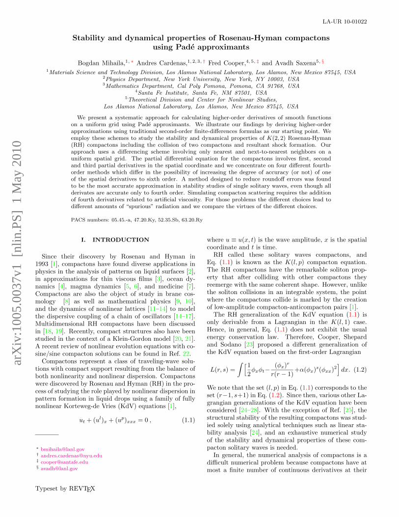
(a) (4,4,4) scheme (b) (6,4,4) scheme
(c) (4,6,4) scheme (d) (4,4,6) scheme
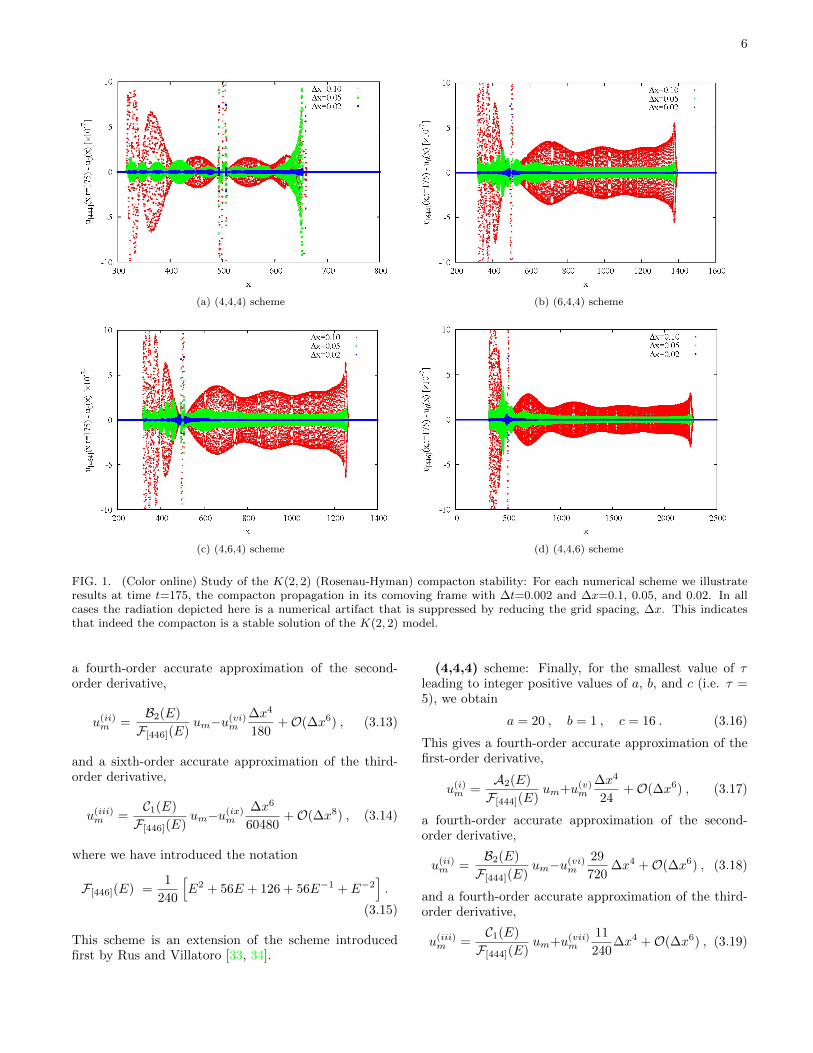
FIG. 1. (Color online) Study of the K(2, 2) (Rosenau-Hyman) compacton stability: For each numerical scheme we illustrateresults at time t=175, the compacton propagation in its comoving frame with ∆t=0.002 and ∆x=0.1, 0.05, and 0.02. In allcases the radiation depicted here is a numerical artifact that is suppressed by reducing the grid spacing, ∆x. This indicatesthat indeed the compacton is a stable solution of the K(2, 2) model.
a fourth-order accurate approximation of the second-order derivative,
u(ii)m =B2(E)
F[446](E)um−u(vi)m
∆x4
180+O(∆x6) , (3.13)
and a sixth-order accurate approximation of the third-order derivative,
u(iii)m =C1(E)
F[446](E)um−u(ix)m
∆x6
60480+O(∆x8) , (3.14)
where we have introduced the notation
F[446](E) =1
240
[E2 + 56E + 126 + 56E−1 + E−2
].
(3.15)
This scheme is an extension of the scheme introducedfirst by Rus and Villatoro [33, 34].
(4,4,4) scheme: Finally, for the smallest value of τleading to integer positive values of a, b, and c (i.e. τ =5), we obtain
a = 20 , b = 1 , c = 16 . (3.16)
This gives a fourth-order accurate approximation of thefirst-order derivative,
u(i)m =A2(E)
F[444](E)um+u(v)m
∆x4
24+O(∆x6) , (3.17)
a fourth-order accurate approximation of the second-order derivative,
u(ii)m =B2(E)
F[444](E)um−u(vi)m
29
720∆x4 +O(∆x6) , (3.18)
and a fourth-order accurate approximation of the third-order derivative,
u(iii)m =C1(E)
F[444](E)um+u(vii)m
11
240∆x4 +O(∆x6) , (3.19)
7
where we have introduced the notation
F[444](E) =1
20
[E2 + E + 16 + E−1 + E−2
]. (3.20)
IV. RESULTS
To compare the quality of the approximations dis-cussed above, we specialize to the case of the K(p, p)equation. In a frame of reference moving with velocityc0, the K(p, p) equation reads
∂u
∂t− c0
∂u
∂x+∂up
∂x+∂3up
∂x3= 0, 1 < p ≤ 3 . (4.1)
For p restricted to the interval 1 < p ≤ 3, the K(p, p)equation allows for a compacton solution, with the simpleform [32, 33, 40]
uc(x, t) = αγ cos2γ[βξ(x, t)
], |ξ(x, t)| ≤ π/(2β) ,
(4.2)where c is the compacton velocity and x0 is the positionof its maximum at t = 0, and we have introduced thenotations ξ(x, t) = x− x0 − (c− c0)t, and
α =2cp
p+ 1, β =
p− 1
2p, γ =
1
p− 1. (4.3)
Numerically, the lack of smoothness at the edge ofthe compacton introduces numerical high-frequency dis-persive errors into the calculation, which can destroythe accuracy of the simulation unless they are explicitlydamped (see e.g. discussion in Ref. [25]). As such, wesolve Eq. (4.1) in the presence of an artificial dissipation(hyperviscosity) term based on fourth spatial derivative,µ∂4u/∂x4, and we choose µ as small as possible to reducethese numerical artifacts while not significantly chang-ing the solution to the compacton problem. We note
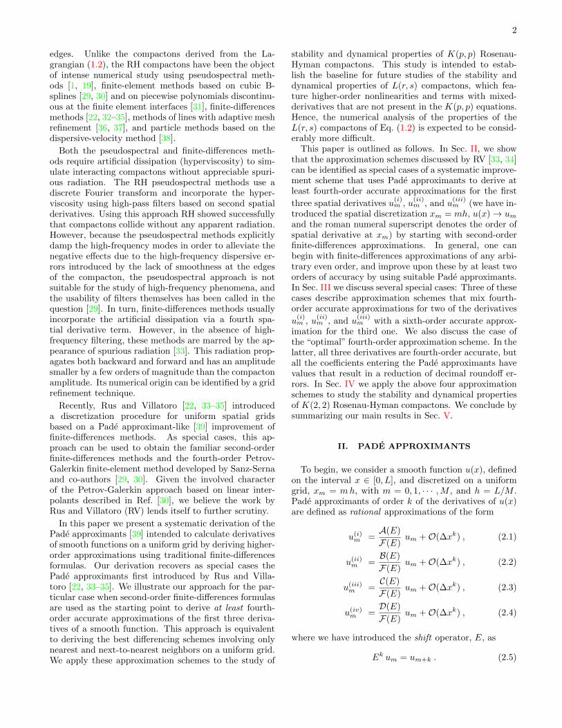
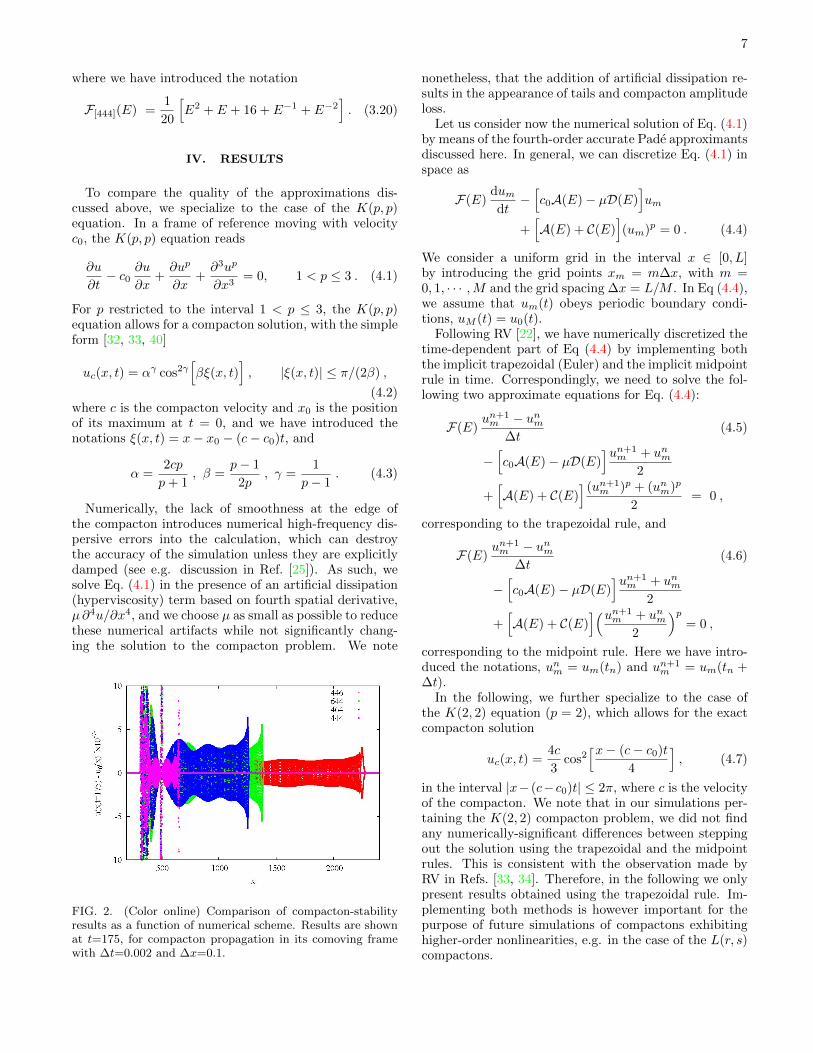
FIG. 2. (Color online) Comparison of compacton-stabilityresults as a function of numerical scheme. Results are shownat t=175, for compacton propagation in its comoving framewith ∆t=0.002 and ∆x=0.1.
nonetheless, that the addition of artificial dissipation re-sults in the appearance of tails and compacton amplitudeloss.
Let us consider now the numerical solution of Eq. (4.1)by means of the fourth-order accurate Pade approximantsdiscussed here. In general, we can discretize Eq. (4.1) inspace as
F(E)dumdt−[c0A(E)− µD(E)
]um
+[A(E) + C(E)
](um)p = 0 . (4.4)
We consider a uniform grid in the interval x ∈ [0, L]by introducing the grid points xm = m∆x, with m =0, 1, · · · ,M and the grid spacing ∆x = L/M . In Eq (4.4),we assume that um(t) obeys periodic boundary condi-tions, uM (t) = u0(t).
Following RV [22], we have numerically discretized thetime-dependent part of Eq (4.4) by implementing boththe implicit trapezoidal (Euler) and the implicit midpointrule in time. Correspondingly, we need to solve the fol-lowing two approximate equations for Eq. (4.4):
F(E)un+1m − unm
∆t(4.5)
−[c0A(E)− µD(E)
]un+1m + unm
2
+[A(E) + C(E)
] (un+1m )p + (unm)p
2= 0 ,
corresponding to the trapezoidal rule, and
F(E)un+1m − unm
∆t(4.6)
−[c0A(E)− µD(E)
]un+1m + unm
2
+[A(E) + C(E)
](un+1m + unm
2
)p= 0 ,
corresponding to the midpoint rule. Here we have intro-duced the notations, unm = um(tn) and un+1
m = um(tn +∆t).
In the following, we further specialize to the case ofthe K(2, 2) equation (p = 2), which allows for the exactcompacton solution
uc(x, t) =4c
3cos2
[x− (c− c0)t
4
], (4.7)
in the interval |x− (c− c0)t| ≤ 2π, where c is the velocityof the compacton. We note that in our simulations per-taining the K(2, 2) compacton problem, we did not findany numerically-significant differences between steppingout the solution using the trapezoidal and the midpointrules. This is consistent with the observation made byRV in Refs. [33, 34]. Therefore, in the following we onlypresent results obtained using the trapezoidal rule. Im-plementing both methods is however important for thepurpose of future simulations of compactons exhibitinghigher-order nonlinearities, e.g. in the case of the L(r, s)compactons.
8
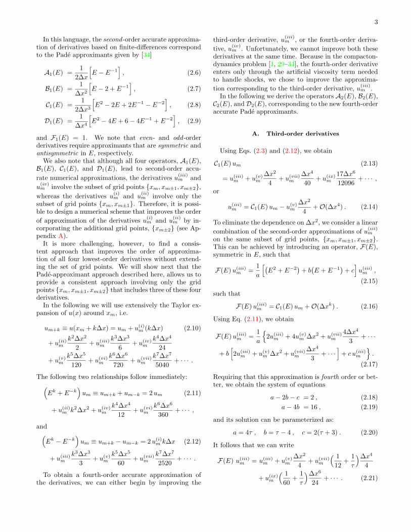
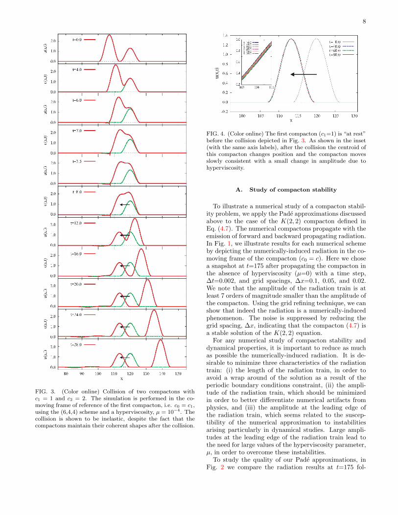
FIG. 3. (Color online) Collision of two compactons withc1 = 1 and c2 = 2. The simulation is performed in the co-moving frame of reference of the first compacton, i.e. c0 = c1,using the (6,4,4) scheme and a hyperviscosity, µ = 10−4. Thecollision is shown to be inelastic, despite the fact that thecompactons maintain their coherent shapes after the collision.
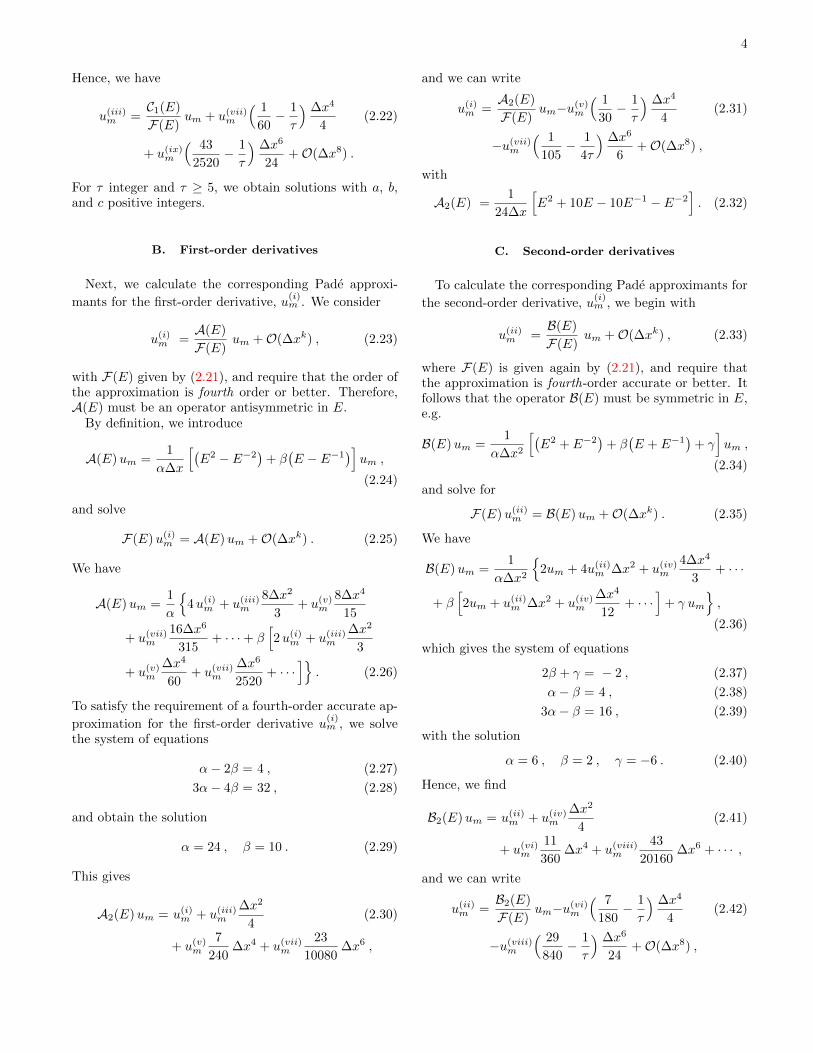
FIG. 4. (Color online) The first compacton (c1=1) is “at rest”before the collision depicted in Fig. 3. As shown in the inset(with the same axis labels), after the collision the centroid ofthis compacton changes position and the compacton movesslowly consistent with a small change in amplitude due tohyperviscosity.
A. Study of compacton stability
To illustrate a numerical study of a compacton stabil-ity problem, we apply the Pade approximations discussedabove to the case of the K(2, 2) compacton defined inEq. (4.7). The numerical compactons propagate with theemission of forward and backward propagating radiation.In Fig. 1, we illustrate results for each numerical schemeby depicting the numerically-induced radiation in the co-moving frame of the compacton (c0 = c). Here we chosea snapshot at t=175 after propagating the compacton inthe absence of hyperviscosity (µ=0) with a time step,∆t=0.002, and grid spacings, ∆x=0.1, 0.05, and 0.02.We note that the amplitude of the radiation train is atleast 7 orders of magnitude smaller than the amplitude ofthe compacton. Using the grid refining technique, we canshow that indeed the radiation is a numerically-inducedphenomenon. The noise is suppressed by reducing thegrid spacing, ∆x, indicating that the compacton (4.7) isa stable solution of the K(2, 2) equation.
For any numerical study of compacton stability anddynamical properties, it is important to reduce as muchas possible the numerically-induced radiation. It is de-sirable to minimize three characteristics of the radiationtrain: (i) the length of the radiation train, in order toavoid a wrap around of the solution as a result of theperiodic boundary conditions constraint, (ii) the ampli-tude of the radiation train, which should be minimizedin order to better differentiate numerical artifacts fromphysics, and (iii) the amplitude at the leading edge ofthe radiation train, which seems related to the suscep-tibility of the numerical approximation to instabilitiesarising particularly in dynamical studies. Large ampli-tudes at the leading edge of the radiation train lead tothe need for large values of the hyperviscosity parameter,µ, in order to overcome these instabilities.
To study the quality of our Pade approximations, inFig. 2 we compare the radiation results at t=175 fol-
9
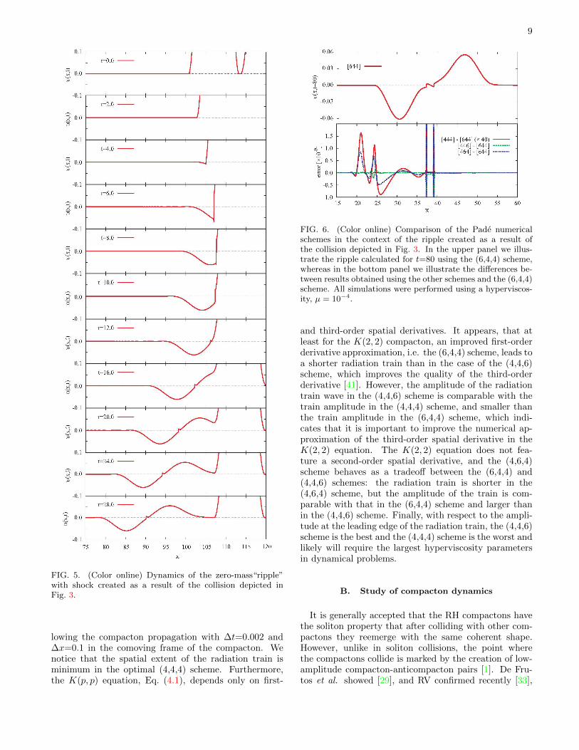
FIG. 5. (Color online) Dynamics of the zero-mass“ripple”with shock created as a result of the collision depicted inFig. 3.
lowing the compacton propagation with ∆t=0.002 and∆x=0.1 in the comoving frame of the compacton. Wenotice that the spatial extent of the radiation train isminimum in the optimal (4,4,4) scheme. Furthermore,the K(p, p) equation, Eq. (4.1), depends only on first-
FIG. 6. (Color online) Comparison of the Pade numericalschemes in the context of the ripple created as a result ofthe collision depicted in Fig. 3. In the upper panel we illus-trate the ripple calculated for t=80 using the (6,4,4) scheme,whereas in the bottom panel we illustrate the differences be-tween results obtained using the other schemes and the (6,4,4)scheme. All simulations were performed using a hyperviscos-ity, µ = 10−4.
and third-order spatial derivatives. It appears, that atleast for the K(2, 2) compacton, an improved first-orderderivative approximation, i.e. the (6,4,4) scheme, leads toa shorter radiation train than in the case of the (4,4,6)scheme, which improves the quality of the third-orderderivative [41]. However, the amplitude of the radiationtrain wave in the (4,4,6) scheme is comparable with thetrain amplitude in the (4,4,4) scheme, and smaller thanthe train amplitude in the (6,4,4) scheme, which indi-cates that it is important to improve the numerical ap-proximation of the third-order spatial derivative in theK(2, 2) equation. The K(2, 2) equation does not fea-ture a second-order spatial derivative, and the (4,6,4)scheme behaves as a tradeoff between the (6,4,4) and(4,4,6) schemes: the radiation train is shorter in the(4,6,4) scheme, but the amplitude of the train is com-parable with that in the (6,4,4) scheme and larger thanin the (4,4,6) scheme. Finally, with respect to the ampli-tude at the leading edge of the radiation train, the (4,4,6)scheme is the best and the (4,4,4) scheme is the worst andlikely will require the largest hyperviscosity parametersin dynamical problems.
B. Study of compacton dynamics
It is generally accepted that the RH compactons havethe soliton property that after colliding with other com-pactons they reemerge with the same coherent shape.However, unlike in soliton collisions, the point wherethe compactons collide is marked by the creation of low-amplitude compacton-anticompacton pairs [1]. De Fru-tos et al. showed [29], and RV confirmed recently [33],
10
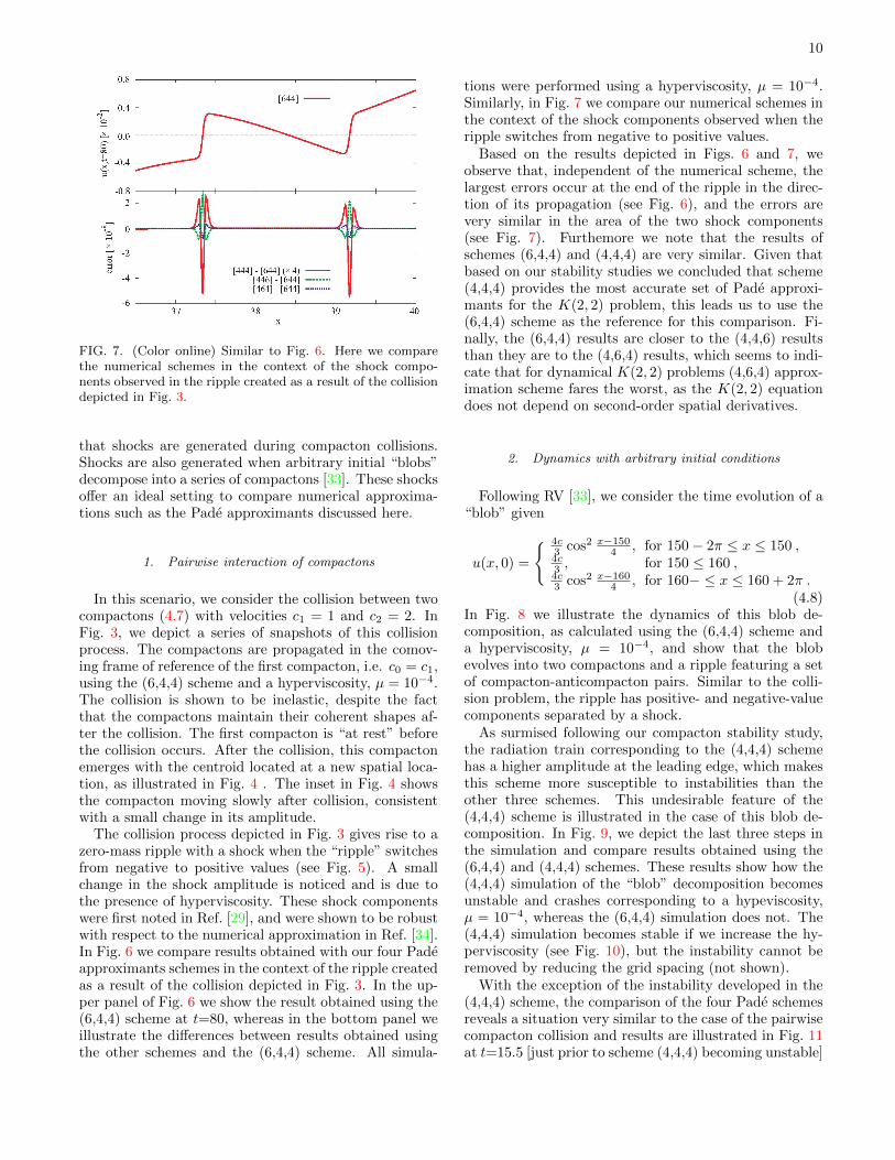
FIG. 7. (Color online) Similar to Fig. 6. Here we comparethe numerical schemes in the context of the shock compo-nents observed in the ripple created as a result of the collisiondepicted in Fig. 3.
that shocks are generated during compacton collisions.Shocks are also generated when arbitrary initial “blobs”decompose into a series of compactons [33]. These shocksoffer an ideal setting to compare numerical approxima-tions such as the Pade approximants discussed here.
1. Pairwise interaction of compactons
In this scenario, we consider the collision between twocompactons (4.7) with velocities c1 = 1 and c2 = 2. InFig. 3, we depict a series of snapshots of this collisionprocess. The compactons are propagated in the comov-ing frame of reference of the first compacton, i.e. c0 = c1,using the (6,4,4) scheme and a hyperviscosity, µ = 10−4.The collision is shown to be inelastic, despite the factthat the compactons maintain their coherent shapes af-ter the collision. The first compacton is “at rest” beforethe collision occurs. After the collision, this compactonemerges with the centroid located at a new spatial loca-tion, as illustrated in Fig. 4 . The inset in Fig. 4 showsthe compacton moving slowly after collision, consistentwith a small change in its amplitude.
The collision process depicted in Fig. 3 gives rise to azero-mass ripple with a shock when the “ripple” switchesfrom negative to positive values (see Fig. 5). A smallchange in the shock amplitude is noticed and is due tothe presence of hyperviscosity. These shock componentswere first noted in Ref. [29], and were shown to be robustwith respect to the numerical approximation in Ref. [34].In Fig. 6 we compare results obtained with our four Padeapproximants schemes in the context of the ripple createdas a result of the collision depicted in Fig. 3. In the up-per panel of Fig. 6 we show the result obtained using the(6,4,4) scheme at t=80, whereas in the bottom panel weillustrate the differences between results obtained usingthe other schemes and the (6,4,4) scheme. All simula-
tions were performed using a hyperviscosity, µ = 10−4.Similarly, in Fig. 7 we compare our numerical schemes inthe context of the shock components observed when theripple switches from negative to positive values.
Based on the results depicted in Figs. 6 and 7, weobserve that, independent of the numerical scheme, thelargest errors occur at the end of the ripple in the direc-tion of its propagation (see Fig. 6), and the errors arevery similar in the area of the two shock components(see Fig. 7). Furthemore we note that the results ofschemes (6,4,4) and (4,4,4) are very similar. Given thatbased on our stability studies we concluded that scheme(4,4,4) provides the most accurate set of Pade approxi-mants for the K(2, 2) problem, this leads us to use the(6,4,4) scheme as the reference for this comparison. Fi-nally, the (6,4,4) results are closer to the (4,4,6) resultsthan they are to the (4,6,4) results, which seems to indi-cate that for dynamical K(2, 2) problems (4,6,4) approx-imation scheme fares the worst, as the K(2, 2) equationdoes not depend on second-order spatial derivatives.
2. Dynamics with arbitrary initial conditions
Following RV [33], we consider the time evolution of a“blob” given
u(x, 0) =
{ 4c3 cos2 x−1504 , for 150− 2π ≤ x ≤ 150 ,4c3 , for 150 ≤ 160 ,4c3 cos2 x−1604 , for 160− ≤ x ≤ 160 + 2π .
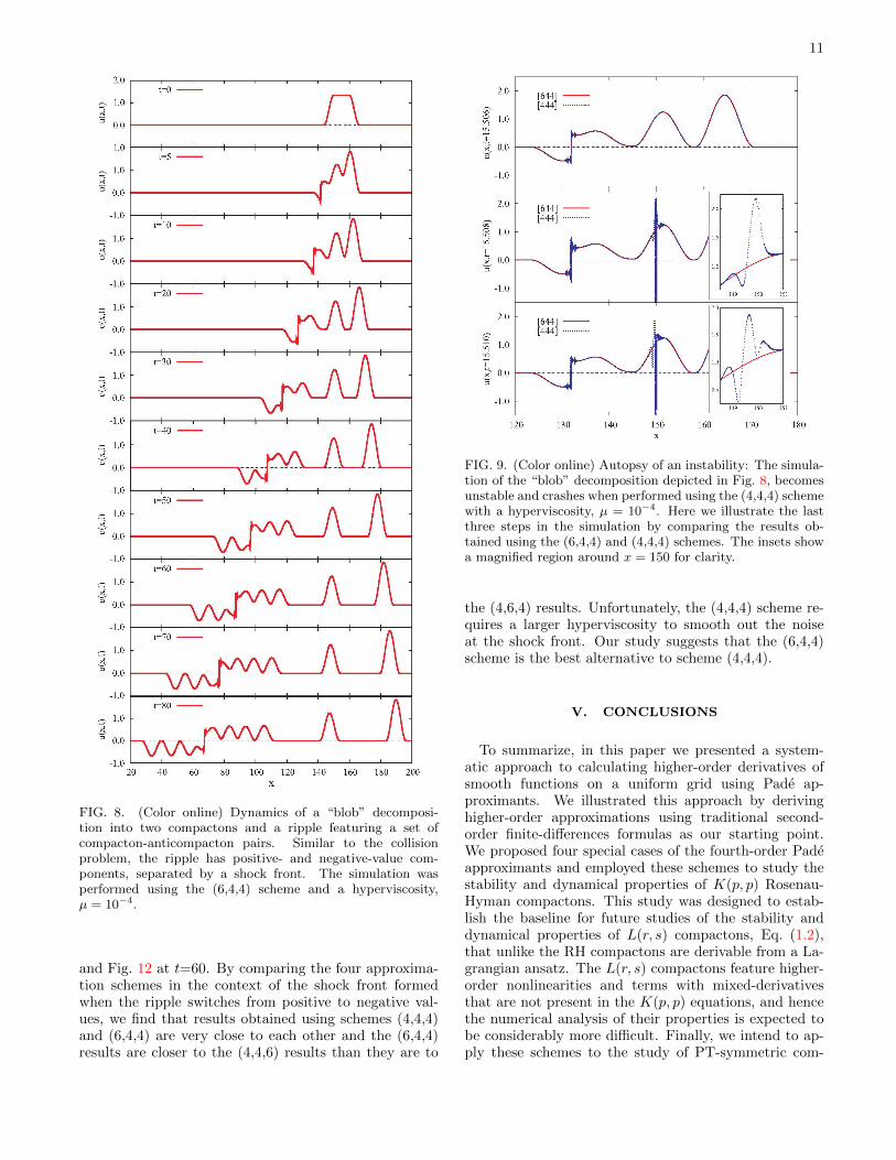
(4.8)In Fig. 8 we illustrate the dynamics of this blob de-composition, as calculated using the (6,4,4) scheme anda hyperviscosity, µ = 10−4, and show that the blobevolves into two compactons and a ripple featuring a setof compacton-anticompacton pairs. Similar to the colli-sion problem, the ripple has positive- and negative-valuecomponents separated by a shock.
As surmised following our compacton stability study,the radiation train corresponding to the (4,4,4) schemehas a higher amplitude at the leading edge, which makesthis scheme more susceptible to instabilities than theother three schemes. This undesirable feature of the(4,4,4) scheme is illustrated in the case of this blob de-composition. In Fig. 9, we depict the last three steps inthe simulation and compare results obtained using the(6,4,4) and (4,4,4) schemes. These results show how the(4,4,4) simulation of the “blob” decomposition becomesunstable and crashes corresponding to a hypeviscosity,µ = 10−4, whereas the (6,4,4) simulation does not. The(4,4,4) simulation becomes stable if we increase the hy-perviscosity (see Fig. 10), but the instability cannot beremoved by reducing the grid spacing (not shown).
With the exception of the instability developed in the(4,4,4) scheme, the comparison of the four Pade schemesreveals a situation very similar to the case of the pairwisecompacton collision and results are illustrated in Fig. 11at t=15.5 [just prior to scheme (4,4,4) becoming unstable]
11
FIG. 8. (Color online) Dynamics of a “blob” decomposi-tion into two compactons and a ripple featuring a set ofcompacton-anticompacton pairs. Similar to the collisionproblem, the ripple has positive- and negative-value com-ponents, separated by a shock front. The simulation wasperformed using the (6,4,4) scheme and a hyperviscosity,µ = 10−4.
and Fig. 12 at t=60. By comparing the four approxima-tion schemes in the context of the shock front formedwhen the ripple switches from positive to negative val-ues, we find that results obtained using schemes (4,4,4)and (6,4,4) are very close to each other and the (6,4,4)results are closer to the (4,4,6) results than they are to
FIG. 9. (Color online) Autopsy of an instability: The simula-tion of the “blob” decomposition depicted in Fig. 8, becomesunstable and crashes when performed using the (4,4,4) schemewith a hyperviscosity, µ = 10−4. Here we illustrate the lastthree steps in the simulation by comparing the results ob-tained using the (6,4,4) and (4,4,4) schemes. The insets showa magnified region around x = 150 for clarity.
the (4,6,4) results. Unfortunately, the (4,4,4) scheme re-quires a larger hyperviscosity to smooth out the noiseat the shock front. Our study suggests that the (6,4,4)scheme is the best alternative to scheme (4,4,4).
V. CONCLUSIONS
To summarize, in this paper we presented a system-atic approach to calculating higher-order derivatives ofsmooth functions on a uniform grid using Pade ap-proximants. We illustrated this approach by derivinghigher-order approximations using traditional second-order finite-differences formulas as our starting point.We proposed four special cases of the fourth-order Padeapproximants and employed these schemes to study thestability and dynamical properties of K(p, p) Rosenau-Hyman compactons. This study was designed to estab-lish the baseline for future studies of the stability anddynamical properties of L(r, s) compactons, Eq. (1.2),that unlike the RH compactons are derivable from a La-grangian ansatz. The L(r, s) compactons feature higher-order nonlinearities and terms with mixed-derivativesthat are not present in the K(p, p) equations, and hencethe numerical analysis of their properties is expected tobe considerably more difficult. Finally, we intend to ap-ply these schemes to the study of PT-symmetric com-
12
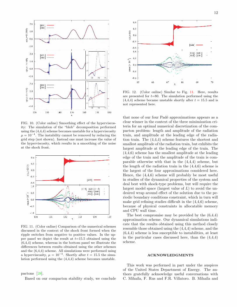
FIG. 10. (Color online) Smoothing effect of the hyperviscos-ity: The simulation of the “blob” decomposition performedusing the (4,4,4) scheme becomes unstable for a hyperviscosityµ = 10−4. The instability cannot be removed by reducing thegrid step (not shown). Instead one must increase the value ofthe hyperviscosity, which results in a smoothing of the noiseat the shock front.
FIG. 11. (Color online) Comparison of the numerical schemesdiscussed in the context of the shock front formed when theripple switches from negative to positive values. In the up-per panel we depict the result at t=15.5 obtained using the(6,4,4) scheme, whereas in the bottom panel we illustrate thedifferences between results obtained using the other schemesand the (6,4,4) scheme. All simulations were performed usinga hyperviscosity, µ = 10−4. Shortly after t = 15.5 the simu-lation performed using the (4,4,4) scheme becomes unstable.
pactons [28].
Based on our compacton stability study, we conclude
FIG. 12. (Color online) Similar to Fig. 11. Here, resultsare presented for t=80. The simulation performed using the(4,4,4) scheme became unstable shortly after t = 15.5 and isnot represented here.
that none of our four Pade approximations appears as aclear winner in the context of the three minimization cri-teria for an optimal numerical discretization of the com-pacton problem: length and amplitude of the radiationtrain, and amplitude at the leading edge of the radia-tion train. The (4,4,4) scheme features the shortest andsmallest amplitude of the radiation train, but exhibits thelargest amplitude at the leading edge of the train. The(4,4,6) scheme has the smallest amplitude at the leadingedge of the train and the amplitude of the train is com-parable otherwise with that in the (4,4,4) scheme, butthe length of the radiation train in the (4,4,6) scheme isthe largest of the four approximations considered here.Hence, the (4,4,6) scheme will probably be most usefulin studies of the dynamical properties of the system anddeal best with shock-type problems, but will require thelargest model space (largest value of L) to avoid the un-desired wrap around effect of the solution due to the pe-riodic boundary conditions constraint, which in turn willmake grid refining studies difficult in the (4,4,6) scheme,because of physical constraints in allocatable memoryand CPU wall time.
The best compromise may be provided by the (6,4,4)approximation scheme. Our dynamical simulations indi-cate that the results obtained using this method closelyresemble those obtained using the (4,4,4) scheme, and the(6,4,4) scheme is less susceptible to instabilities, at leastin the particular cases discussed here, than the (4,4,4)scheme.
ACKNOWLEDGMENTS
This work was performed in part under the auspicesof the United States Department of Energy. The au-thors gratefully acknowledge useful conversations withC. Mihaila, F. Rus and F.R. Villatoro. B. Mihaila and
13
F. Cooper would like to thank the Santa Fe Institute for its hospitality during the completion of this work.
[1] P. Rosenau and J.M. Hyman, Phys. Rev. Lett. 70, 564(1993).
[2] A. Ludu and J.P. Draayer, Physica D 123, 82 (1998).[3] A.L. Bertozzi and M. Pugh, Commun. Pure Appl. Math.
49, 85 (1996).[4] R.H.J. Grimshaw, L.A. Ostrovsky, V.I. Shrira, and Y.A.
Stepanyants, Surv. Geophys. 19, 289 (1998).[5] G. Simpson, M. Spiegelman, and M.I. Weinstein, Non-
linearity 20, 21 (2007).[6] G. Simpson, M.I. Weinstein, and P. Rosenau, Discrete
and Series B 10, 903 (2008).[7] V. Kardashov, S. Einav, Y. Okrent, and T. Kardashov,
Discrete Dyn. Nat. Soc. 2006, Art. 98959 (2006)[8] C. Adam, N. Grandi, P. Klimas, J. Sanchez-Guillen, and
A. Wereszczynski, J. Phys. A 41, 375401 (2008).[9] A.S. Kovalev and M.V. Gvozdikova, Low Temp. Phys.
24, 484 (1998).[10] E.C. Caparelli, V.V. Dodonov, and S.S. Mizrahi, Phys.
Scr. 58, 417 (1998).[11] S. Dusuel, P. Michaux, and M. Remoissenet, Phys. Rev.
E 57, 2320 (1998).[12] J.C. Comte, Chaos Solitons Fractals 14, 1193 (2002).[13] J.C. Comte and P. Marquie, Chaos Solitons Fractals 29,
307 (2006).[14] J.E. Prilepsky, A.S. Kovalev, M. Johansson, and Y.S.
Kivshar, Phys. Rev. B 74, 132404 (2006).[15] P. Rosenau and A. Pikovsky, Phys. Rev. Lett. 94, 174102
(2005).[16] A. Pikovsky and P. Rosenau, Physica D 218, 56 (2006).[17] P. Rosenau, Phys. Lett. A 275, 193 (2000).[18] P. Rosenau, Phys. Lett. A 356, 44 (2006).[19] P. Rosenau, J.M. Hyman, and M. Staley, Phys. Rev. Lett.
98, 024101 (2007).[20] P. Rosenau and E. Kashdan, Phys. Rev. Lett. 101,
264101 (2008).[21] P. Rosenau and E. Kashdan, Phys. Rev. Lett. 104,
034101 (2010).[22] F. Rus and F.R. Villatoro, Appl. Math. Comput. 215,
1838 (2009).[23] F. Cooper, H. Shepard, and P. Sodano, Phys. Rev. E 48,
4027 (1993).[24] A. Khare and F. Cooper, Phys. Rev. E 48, 4843 (1993).[25] F. Cooper, J.M. Hyman, and A. Khare, Phys. Rev. E 64,
026608 (2001).[26] B. Dey and A. Khare, Phys. Rev. E 58, R2741 (1998).[27] F. Cooper, A. Khare, and A. Saxena, Complexity 11, 30
(2006)[28] C. Bender, F. Cooper, A. Khare, B. Mihaila, And A.
Saxena, Pramana – J. Phys. 75, 375 (2009)[29] J. De Frutos, M.A. Lopez-Marcos and J.M. Sanz-Serna,
J. Comput. Phys. 120, 248 (1995).[30] J.M. Sanz-Serna and I. Christie, J. Comput. Phys. 29,
94 (1981).[31] D. Levy, C.-W. Shu, and J. Yan, J. Comput. Phys. 196,
751 (2004).[32] M.S. Ismail and T.R. Taha, Math. Comput. Simul. 47,
519 (1998).[33] F. Rus and F.R. Villatoro, Math. Comput. Simul. 76,
188 (2007).[34] F. Rus and F.R. Villatoro, J. Comput. Phys. 227, 440
(2007).[35] F. Rus and F.R. Villatoro, Appl. Math. Comput. 204,
416 (2008).[36] P. Saucez, A. Vande Wouwer, W.E. Schiesser, and P.
Zegeling, J. Comput. Appl. Math. 168, 413 (2004).[37] P. Saucez, A. Vande Wouwer, and P. Zegeling, J. Com-
put. Appl. Math. 183, 343 (2005).[38] A. Chertock and D. Levy, J. Comput. Phys. 171, 708
(2001).[39] G.A. Baker, Jr. and P.R. Graves-Morris, Pade Approxi-
mants, (Cambridge University Press, Cambridge, 1995).[40] P. Rosenau, Physica D 123, 525 (1998).[41] A better analysis of the quality of these numerical
schemes can be done using the analytical approximationof the group velocity of the radiation train discussed inRef. 34 and will be carried out in the future.
Appendix A
In this appendix we discuss the derivation of fourth-order accurate approximations for the first- and second-order derivatives of a smooth function.
To derive a fourth-order accurate approximation of thefirst-order derivative, we begin by introducing the oper-ator
A1(E)um =1
α∆x
[(E2 − E−2
)+ β
(E − E−1
)]um ,
(A1)
and ask that the following relation is fulfilled:
u(i)m = A1(E)um +O(∆x4) . (A2)
We have
A1(E)um =1
α
{4u(i)m + u(iii)m
8∆x2
3+ u(v)m
8∆x4
15
+ u(vii)m
16∆x6
315+ · · ·+ β
[2u(i)m + u(iii)m
∆x2
3
+ u(v)m∆x4
60+ u(vii)m
∆x6
2520+ · · ·
]}. (A3)
To satisfy the requirement of a fourth-order accurate ap-
proximation for the first-order derivative u(i)m , we solve
the system of equations
α− 2β = 4 , (A4)
β = − 8 , (A5)
and obtain the solution
α = −12 , β = −8 . (A6)
14
This gives
u(i)m = A1(E)um + u(v)m∆x4
30+O(∆x6) , (A7)
with
A1(E) = − 1
12∆x
[E2 − 8E + 8E−1 − E−2
]. (A8)
Similarly, to derive a fourth-order accurate approxi-mation for the second-order derivative we introduce theoperator
B1(E)um =1
α∆x2
[(E2 + E−2
)+ β
(E + E−1
)+ γ]um ,
(A9)
and seek α, β, and γ such that
u(ii)m = B1(E)um +O(∆x4) . (A10)
We have
B1(E)um =1
α∆x2
{2um + 4u(ii)m ∆x2 + u(iv)m
4∆x4
3+ · · ·
+ β[2um + u(ii)m ∆x2 + u(iv)m
∆x4
12+ · · ·
]+ γ um
},
(A11)
which gives the system of equations
2β + γ = − 2 , (A12)
α− β = 4 , (A13)
3α− β = 0 , (A14)
with the solution
α = −2 , β = −6 , γ = 10 . (A15)
Hence, we obtain
B1(E) = − 1
2∆x2
[E2 − 6E + 10− 6E−1 + E−2
].
(A16)
and
u(ii)m = B1(E)um + u(vi)m
5
12∆x4 +O(∆x6) . (A17)


