Stability properties of stochastic nOIse - CORE

Stability properties of stochastic

differential equations driven by Levy .

nOIse

Michailina Siakalli

Thesis submitted to the University of Sheffield for the degree of

Doctor of Philosophy

Department of Probability and Statistics

School of Mathematics and Statistics

University of Sheffield

Februa.ry 2009

Abstract

The main aim of this thesis is to examine stability properties of the solutions to

stochastic differential equations (SDEs) driven by Levy noise.

Using key tools such as Ito's formula for general semimartingales, Kunita's moment

estimates for Levy-type stochastic integrals, and the exponential martingale inequality,

we find conditions under which the solutions to the SDEs under consideration are stable

in probability, almost surely and moment exponentially stable. In addition, stability

properties of stochastic functional differential equations (SFDEs) driven by Levy noise

are examined using Razumikhin type theorems.

In the existing literature the problem of stochastic stabilization and destabilization of

first order non-linear deterministic systems has been investigated when the system is

perturbed with Brownian motion. These results are extended in this thesis to the case

where the deterministic system is perturbed with Levy noise. We mainly focus on

the stabilizing effects of the Levy noise in the system, prove the existence of sample

Lyapunov exponents of the trivial solution of the stochastically perturbed system, and

provide sufficient criteria under which the system is almost surely exponentially stable.

From the results that are established the Levy noise plays a similar role to the Brownian

motion in stabilizing dynamical systems.

We also establish the variation of constants formula for linear SDEs driven by Levy

noise. This is applied to study stochastic stabilization of ordinary functional differential

equation systems perturbed with Levy noise.

Acknowledgements

"True wisdom comes to each of us when we realize how little we understand about life,

ourselves, and the world around us. Wisdom begins in wonder". (attributed to Socrates)

First of all my deepest gratitude to my supervisor Professor David Applebaum for

his patience, precious advice and comments, guidance and help through the last three

years. Special thanks to him that besides being an enthusiastic tutor, he was of warm

personality. Also I would like to thank the University of Sheffield for funding me through

the completion of my PhD.

The list of people that I would like to thank could be too long. I would like to thank

all the friends in Sheffield who made my time enjoyable and through chats, dinners and

moments of good humour, gave me the strength to continue. Special thanks to Mark

Eastlick, Sammy" Neil Rashid, Lina Dib, Irene Eleta Mogollon and GioIa Karamitrou.

There were people that even not being close to me in distance, helped me to get through

difficult periods during the last three years. I am really grateful to Maria Papavasiliou,

Margarita Zachariou and Petros Kountouris. Special thanks to Vangelis Therapontos

for his constant support and encouragement.

Last but not least I am very grateful to my family, and especially to my beloved mother

and father Maria and Giorgos Siakallis, to whom I dedicate this work. They were always

by my side, supporting me and instilling confidence in me. What I will write for them

definitely is not enough. Without their endless support and love, I do not think I was

going to be able to finish this thesis. Thank you!

ii

Contents

1 Introduction to Levy Processes, Stochastic Differential Equations

(SDEs) and Stability Theory 1

1.1 Introd uction. . . . . . . . .

1.2 Levy processes: basic definitions and properties .

1.2.1 Some examples of Levy processes ..

1.2.2 Levy-Ito decomposition ..

1.3 Stochastic Calculus - Ito's formula

1.4 Stochastic Differential Equations - SDEs ..

1.5 Stability Theory of SDEs

1. 6 Overview ....... .

2 Properties of linear SDEs

2.1 Introduction ...... . .................

1

1

4

5

7

12

14

20

22

22

2.2 Variation of constants formula for an SDE driven by a Levy process 22

2.3 Special case: Variation of constants formula for an SDE driven by a

Poisson process ................................

3 Stability of SDEs

3.1 Introduction ..

3.2 LP Estimates

3.2.1 Exponential martingale inequality

3.3 Stability in probability ....... .

3.4 Almost surely asymptotic estimates.

iii

38

40

40

40

43

48

50

3.5 Moment exponential stability . . . . . . . . . . . . . . . . . . . . . . .. 64

4 Stochastic Stabilization and Destabilization

4.1 Introduction .................. .

4.2 Existence and uniqueness theorem for Levy driven SDEs with locally

Lipschitz coefficients

4.3 Some useful results.

4.4 Stabilization of a system by a compensated Poisson integral .

4.5 Stabilization by Poisson noise ....... .

4.6 Stabilization of SDEs driven by Levy noise

4.6.1 A special case of an SDE driven by Levy noise

4.7 Stochastic stabilization of linear systems . . . . . .

4.8 Perturbation of non-linear deterministic systems

4.8.1 Stabilization ................ .

4.8.2 Stochastic destabilization of non-linear systems ...

75

75

77

83

85

89

93

95

98

101

101

104

5 Stochastic Functional Differential Equations (SFDEs) driven by Levy

noise 110

5.1 Introduction. ................ 5.2 Existence and uniqueness of solutions

110

111

5.3 Razumikhin type theorems for stochastic functional differential equations 113

5.4 Stochastic differential delay equations ....

5.5 Stabilization of SFDEs by a Poisson process.

A Existence and uniqueness of SFDEs

B A useful lemma

Bibliography

iv

120

123

129

136

137

Notation and Terminology

N = {I, 2, ... } and ~+ = [0,00).

~d is d-dimensional Euclidean space, where dEN. Its elements x = (Xl, X2, ••• , Xd) are

vectors, with Xi E ~ for each I :5 i :5 d. The Euclidean inner-product in ~d between

two vectors x, y E ~d is denoted by (x, y) and is defined as

d

(x, y) = L XiYi,

i=l

or as xT y where xT denotes the transpose of the vector x, and the associated norm is

(d) ~

Ixl = (x, x)~ = ~Xi2 •

'/.=1

Md,m(~) will denote the space of all real-valued d x m matrices. We let Md(~) denote Md,d(~).

The trace of A E Md(~) is shortened to trA. 1

We denote by IIDII = (L:f=l L:~l DlJ)"2 where D E Md,m(~). Note that IIDII

is the Hilbert-Schmidt norm of a d x m matrix D i.e. IIDII = Jtr(DT D) and if

D is d x d symmetric matrix, it is well known that IIDII = maxi=1,2, ... ,d IAil where

{ Ai, i = 1, 2, ... ,d} are the eigenvalues of the matrix D.

Also denote by IIDlll the matrix norm defined by IIDlh = sup {IIDyll : Ilyll = I} where D is a d x d matrix.

The kernel of a matrix A E Md,m(~) is denoted throughout the thesis as Ker(A) and by I we denote the identity matrix.

For a matrix A E Md(~) we say that is P9sitive definite if yT Ay > 0 for all non-zero y E JRd.

In this thesis the Einstein summation convention is used, wherein summation is

understood with respect to repeated upper and lower indices e.g. if x, y E ~d and

v

d

A;Xiyj = L A;Xiyj = (x, Ay). i,j=l

#S means the number of elements in the set S.

se denotes the complement of a set Sand S denotes the closure in some topology.

'Almost surely' is shorthanded to a.s. and 'almost everywhere' to a.e.

Also we denote a A b = min{a, b} and a V b = max{a, b} for a, bE JR.

We also need to define Cn(JRd), the space of n-times differentiable functions from JRd to

JR, all of whose derivatives are continuous. If V E C2(JRd j JR) then we denote at x E JRd,

(8V(x)) = (81 V(x), ... , 8dV(X))T where 8i V(x) is the i-th first order partial derivative

and (8i 8j V)(x) denotes a~:¥Xj (x).

Throughout this thesis for each x E JRd, c> 0 we denote Be(x) = {y E JRd : Iy - xl < c},

Be(X) = Be(x) \ {O} and Be = Be(O), Be = Be(O).

Let (S, F, J-L) be a measure space and let 1 :5 p < 00. We denote by V(S, F, J-Lj JRd)

the Banach space of all equivalence classes of mappings f : S -+ JRd which agree almost

everywhere (with respect to the meaSure J-L) and for which Ilfllp < 00 where II· lip is the following norm: .

LP(Sj JRd) is a shorthand for V(S, F, J-Lj JRd).

The Borel a-algebra of a Borel set A ~ JRd is denoted by B(A).

Let f : JRd -+ JR. Then limsTt f(8) = k means lims-+t,s<t f(8) = k, while lims.Lt f(8) = k

implies lims-+t,s>t f(8) = k.

We say that f : JR+ -+ JRd is cadla,g (continue d droite avec de8 limite8 d gauche) if it

is right continuous with left limits and we denote the left limit at each point t > 0 by

f(t-) = li~sTt f(8).

Let 7 ~ O. V([-7, O]j JRd) denotes the space of cadlag mappings from [-7,0] to JRd.

We denote by ej the unit column vector, i.e. ej = (0,0, ... ,0,1 (j), 0, ... ,O)T.

We define by ox(A) the Dirac mass concentrated at x E JRd

{

I if x E A ox(A) = 0

if x ~ A,

vi

lA is the indicator function of the Borel set A so

{

I if x E A lA(X) =

o if x (j. A.

vii

.:>

Chapter 1

Introduction to Levy Processes,

Stochastic Differential Equations

(SDEs) and Stability Theory

1.1 Introduction

This chapter falls in~o two parts. The first, is devoted to stochastic analysis of

Levy processes, while the second concerns stability theory. The former provides the

appropriate mathematical tools that are needed to understand the concepts that will be

developed in this thesis for the study of the stability of stochastic differential equations

(SDEs) driven by Levy processes. The latter gives some historical background and the

appropriate mathematical mechanisms needed to develop stability theory.

1.2 Levy processes: basic definitions and properties

In this section we provide a brief introduction to the fundamentals of Levy processes

theory.

Let F be a a-algebra of a given set O. A family (Ft , t ~ 0) of sub a-algebras of F is

called a filtration if

whenever s ~ t.

Assume that we are given a filtered probability space (0, F, (Ft , t ~ 0), P) that satisfies

the "usual hypotheses":

(a) Completeness: Fo contains all sets of P-measure zero.

1

(b) The filtration is right continuous, Ft = Ft+ where Ft+ = n€>o Ft+€.

All random variables that are used in this thesis are considered to be defined on the

same probability space.

Let X = (X(t), t ~ 0) on ]Rd be a stochastic process defined on (0" F, P). Then X is adapted to the filtration (Ft, t ~ 0) (or Ft-adapted) if

X(t) is Ft-measurable for each t ~ O.

If X is Ft-adapted and also satisfies for each t .~ 0 the integrability reiquirement

E(IX(t)1) < 00 then it is a martingale if, for all 0 ~ s < t < 00,

E(X(t)IFs) = X(s) a.s.

Levy processes, named in honor of the French mathematician Paul Levy who first

studied them in the 1930s, are stochastic processes with stationary and independent

increments. They are the simplest class of processes having continuous paths that are

interrupted with jump discontinuities of random size that appear at random times.

Very important examples of Levy processes are Brownian motion which has continuous

sample paths, the Poisson process, the compound Poisson process, stable processes,

su bordinators and interlacing processes. Also a mixture of a Brownian motion and

an independent compound Poisson process can give rise to a Levy process and they

constitute an important class of jump-diffusion processes. In addition Levy processes

form an important class of semimartingales (see Applebaum [1] pp. 115).

A formal definition follows.

Definition 1.2.1 The process X = (X(t), t ~ 0) is a Levy process if it is adapted to

the filtration (Ft, t ~ 0) and the following conditions are satisfied.

(i) X(O) = 0 almost surely,

(ii) each X(t) - X(s) is independent of Fs, V 0 ~ s < t < 00,

(iii) X has stationary increments i.e. X(t) -X(s) has the same distribution as X(t- s),

for each 0 ~ s < t < 00,

(iv) X is stochastically continuous: for all a > 0 and for all s ~ 0

limP[lX(t) - X(s)1 > a] = O. t-s .

Under these conditions, every Levy process X has a cadlag modification and is itself a

Levy process (see e.g. Applebaum [1] Theorem 2.1.7 pp. 74). For the rest of the thesis

we will always consider this modification.

Historically the first investigations into the structure of Levy processes can be tracked

2

back to the late 1920s with the study of infinitely divisible distributions. The general

structure of these was gradually discovered by de Finetti, Kolmogorov, Levy and Ito and

an important landmark is the celebrated Levy-Khintchine formula. This formula gives a

characterization of the infinite divisible probability measures through their characteristic

functions. In the following we will present the Levy-Khintchine formula but first we need

some definitions quoted by Applebaum [1] Chapter 1.

Here M 1 (lRd) denotes the set of all Borel probability measures on IRd.

The convolution of two probability measures J-Li E Ml(IRd), for i = 1,2 is defined as

where A E B(JRd). Also define (I-£)*n = 1-£* ... *1-£ (n times). Then 1-£ E Ml(JRd) is infinitely

divisible if 1-£ has a convolution nth root i.e. if there exists a measure J-Ll/n E Ml (JRd)

for which (J-Ll/n)*n = J-L.

The characteristic function of J-L E M 1 (]Rd) is defined as

where U E JRd.

Now, let v be a Borel measure defined on IRd \ {O} = {x E ]Rd, x i= O}.

Then v is a Levy measure if

r (lyl2 1\ l)v(dy) < 00. JRd\{O}

The Levy-Khintchine formula can now be introduced.

Theorem 1.2.2 (Levy-Khintchine formula)

(1.1)

A Borel probability measure J-L on]Rd is infinitely divisible if there exists a vector b E ]Rd,

a non-negative definite symmetric d x d matrix A and a Levy measure v on ]Rd \ {O} such that, for all U E ]Rd, the characteristic function of J-L admits the representation

<P1'{u) = exp {i(b, u) - ~(u, Au) + Ld\{O} [ei(u,y) - 1 - i{u, y) IB{Y) 1 v{dy) } (1.2)

where B = {y E ]Rd : 0 < Iyl < I}.

Conversely any mapping of the form (1.2) is the characteristic function of an infinitely

divisible probability measure on ]Rd.

For a proof see Sato [42] Theorem 8.1 pp. 37-45.

3

The triple (b, A, v) is called the characteristics of J-L.

Remark 1.2.3 The integral in the Levy-Khintchine formula (1.2) converges. The

integrand is 0(y2) as Iyl ~ 0 and is 0(1) as Iyl ~ 00. Hence, condition (1.1) is a

sufficient condition for the integral to converge.

Now, the connection between the Levy-Khintchine formula and Levy processes is that

each of the random variables comprising a Levy process is infinitely divisible due to

the stationarity and independence of the increments. Hence, the distribution of a Levy

process is determined by the form that the Levy-Khintchine formula can take. Each

X(t) has characteristics (tb, tA, tv) where the (b, A, v) are the characteristics of X(l).

Also the triple (b, A, v) is sufficient to determine some of the sample path properties of

a Levy process e.g. if v = 0 then X has a continuous sample paths (a.s.). For further

details we refer to Sato [42], Section 21 and Kyprianou [27], Chapter 2 pp. 54-55.

1.2.1 Some examples of Levy processes

(1) Brownian motion: A standard Brownian motion B = (B(t), t ~ 0) is a Levy

process on IRd such that

(Bl) B(t) 1'.1 N(O, tI) for each t ~ 0,

(B2) B has continuous sample paths.

The characteristic function of a standard Brownian motion is given by

for each U E IRd , t ~ O.

(2) Poisson process: Let N = (N(t), t ~ 0) be a Poisson process with intensity A > O.

It is a Levy process with non-negative integer values. For each t > 0, N(t) follows a

Poisson distribution with parameter At so that

for each n = 0, 1,2, ....

A Poisson process has piecewise constant paths on each finite time interval and at the

random times

Tn = irif {t ~ OJ N(t) = n}

4

it has jumps of size 1. Its characteristic function is given by

cPN(t)(U) = exp [.At (e iU - 1)] ,

for each U E JRd, t ~ O.

(3) Compound Poisson process: Let (N(t), t ~ 0) be a Poisson random process

with intensity A > 0 and let (U (m), mEN) be a sequence of independent, identically

distributed random variables on JRd, independent of N and defined on the probability

space ([2, F, P) with common law /-Lu. The compound Poisson process Z = (Z(t), t ~ 0)

is a Levy process, where for each t ~ 0

N(t)

Z(t) = L U(k). k=l

The characteristic function of a compound Poisson process is

for each U E JRd, t ~ 0 and we can deduce that the Levy measure for Z is .A/-Lu.

For further examples of processes that belong to the class of Levy processes see e.g.

Applebaum [1] ..

1.2.2 Levy-Ito decomposition

Before we introduce another important tool in the theory of Levy processes, the Levy

Ito decomposition (see Ikeda-Watanabe [18] pp. 65 and Applebaum [1] pp. 108), we

need to give some definitions.

We say that A E 8(JRd\ {O}) is bounded below if 0 ~ A.

Let S be a subset of JRd\ {O} and N be an integer-valued random measure on U = JR+ X S

(for the definition of random measures see Applebaum [1] pp. 89). Then N is a Poisson

random measure if

(1) For each t ~ 0 and A E 8(S) that is bounded below, N(t, A) is Poisson distributed,

(2) For each tl, ... , tn E JR+ and each disjoint family AI, A 2 , ••• ,~An E 8(S) that are

bounded below, then the random variables N(tl' AI)"." N(tn, An) are independent.

Its intensity measure is defined as .A(A) = E(N(l, A)) for all A E 8(S) that are bounded

below.

Now let S = JRd\ {O}.

The jump process associated to a Levy process X is defined by ~X =. (~X(t), t ~ 0)

5

where

~X(t) = X(t) - X(t-)

for each t ;::: O.

To count the jumps of the Levy process X we define for each E E B(JRd\ {O})

N(t, E) = # {O ::; s ::; tj ~X(s) E E} = L IE (~X(s)) . o~s~t

For each w E 0, t ;::: 0 the set function E ~ N(t, E)(w) is a counting measure on

B(JRd\ {O}). Define an associated Borel measure lI(') = E(N(l, .)) (as in Applebaum [1] pp. 87). N is a Poisson random measure, and its intensity measure is Leb 0 lI, where

Leb denotes Lebesgue measure on JR+. We also define the compensated Poisson random

measure by

N(t, E) = N(t, E) - tll(E).

Note that (N(t, E), t ;::: 0) is a martingale whenever lI(E) < 00.

For further details we refer to Applebaum [1] pp. 85-91.

For the rest of this subsection we denote by BA = (BA(t), t ;::: 0) in JRd, the Gaussian

process defined for each t ;::: 0 by

BA(t) = (Bl(t), ... , B~(t)) ,

where for each i = 1,2, ... , d

m

B~(t) = LCTjBj(t) j=l

and for each j = 1,2, ... , m, Bj is a one-dimensional Brownian motion, A E Md(JR)

is a non-negative definite symmetric matrix, CT E Md,m(JR) is a real-valued matrix, the

square root of A such that aaT = A. The process BA = (BA(t), t ;::: 0) is a Levy process

where for each t ;::: 0, BA(t) rv N(O, tA). We call the process BA = (BA(t), t ;::: 0)

Brownian motion with convariance A.

Now the Levy-Ito decomposition describes th~ sample paths of a Levy process as a sum

of a continuous part and jump parts. It effectively tells us that it can be decomposed

into a Brownian motion with drift which is the continuous part, a compensated Poisson

integral which represents the "small jumps" and a Poisson integral that describes the

"large jumps" and is a compound Poisson process.

6

Theorem 1.2.4 (Levy-Ito decomposition)

Every Levy process (X(t), t ~ 0) has the sample path decomposition

X(t) = bt + BA(t) + ( yN(t, dy) + ( yN(t, dy) J1yl<1 J1yl?1

(1.3)

for each t ~ 0, where b E JRd, (BA' t ~ 0) is a Brownian motion with covariance matrix

A and N is an independent Poisson random measure defined on JR+ x (JRd \ {O}) with

intensity measure Leb ® v.

Proof: See e.g. Applebaum [1] pp. 104-108.

Note that the three processes in (1.3) are all independent and the decomposition is

unique (see Kunita [25] Theorem 2.7 pp. 327).

In general a Levy process may not be a martingale, or even integrable but there are

some important examples of Levy processes that possess this property; for instance if a

Levy process has a zero mean then it is a martingale e.g. consider standard Brownian

motion or the compensated Poisson process with intensity A > O.

For a more detailed treatment of the properties of Levy processes we refer to Applebaum

[1], Sato [42], Protter [40] and Kyprianou [27].

1.3 Stochastic Calculus - Ito's formula

In the following some basic tools from stochastic analysis theory and stochastic calculus

will be introduced. These are needed for the purposes of this work. We will follow the

definitions and notation of Applebaum [1].

Throughout this thesis, unless otherwise specified we assume that we are given an

m-dimensional standard Ft-adapted Brownian motion B = (B(t), t ~ 0) with each

B (t) = (B 1 (t), ... , B m (t)) and an independent Ft-adapted Poisson random measure N

defined on JR+ x (JRd \ {O}) with compensator N and intensity measure v, where we will

assume that 1/ is a Levy measure.

Let E E B(JRd \ {O}) and 0 < T < 00. In order to assure the existence of stochastic

integrals for which the integrator is a Levy proGess, we need to define two spaces P2(T, E)

and P2 (T). The space P2 (T, E) is defined as the linear space of all predictable mappings

H : [0, T] x E x n ~ JRd (for the definition of predictability see Applebaum [1] pp. 192)

which satisfy

P [loT k IH(s, YWv(dy)ds < 00] = 1.

7

The space P2 (T) is the linear space of all predictable mappings F : [0, T] x n -+ ]Rd for

which P [J[ IF(t)12dt < 00] = 1. For further details about stochastic integration we

refer to Applebaum [1] Chapter 4.

For the rest of the thesis we take E = Be where 0 < C :::; 00 plays the role of maximum

allowable jump size. This parameter indicates what we mean by small and large jumps,

and in the case where we want to consider small and large jumps under the same footing

we take C = 00.

A result that will playa vital role in this thesis is the celebrated Ito's formula. As will

be revealed in the following chapters, it is a key technique applied to SDEs in order to

establish stability.

Here we will give Ito's formula for a Levy-type stochastic integral, with stochastic

differential

dY(t) = C(t)dt + F(t)dB(t) + r H(t, y)N(dt, dy) + r K(t, y)N(dt, dy) (1.4) J1yl <e J1yl ~e

where for all t ~ 0,1 :::; i :::; d, 1 :::; j :::; m, (Ci)1/2, Fj E P2(t), Hi E P2(t, E) and K is

predictable. The construction of these integrals can be found in Applebaum [1] Chapter

4, pp. 205-212.

It is easily verified that Levy-type stochastic integrals are semimartingales. Hence, the

general Ito's formula for semimartingales can be applied (see e.g. Protter [40], pp. 271).

Using algebra it is straightforward to prove the equivalence between Ito's formula for

general semimartingales and Ito's formula in the form that follows. In this form it

can be found in Ikeda-Watanabe [18] and Applebaum [1] pp. 226. Although it first

appeared many years ago it is only in the l~t ten years that the importance of writing

Ito's formula in this way has been appreciated .

. First we need to define the quadratic variation process [Y, Y] = ([Y, Y](t), t ~ 0) for

Y = (Y(t), t ~ 0) where Y as in (1.4). It is a d x d matrix-valued adapted process and

its (i, j)th entry, where 1 :::; i, j :::; d, is defined by

[Yi, yi](t) = [Yj, Yj](t) + L ~yi(s)~yi(s), (1.5) O::=;s::=;t

where Yc is the continuous part of Y defined "by Yj(t) = J~ Fk(s)dBk(s) + J~ Ci(s)ds for each t ~ 0, 1 :::; i :::; d, 1 :::; k :::; m.

By Applebaum [1] corollary 4.4.9 pp. 228, for each t ~ 0 [yi, yi](t) is almost surely

8

finite, and we have

m t . t

[yi, yi](t) = L r F~(s)Ft(s)ds + r r Hi(s,y)Hi(s,y)N(ds,dy) k=l Jo Jo J1yl<c

+ rt r Ki(S, y)Ki (s, y)N(ds, dy). Jo J1yl?c

For the validity of Ito's formula we need to impose the following local bounded ness

constraint on the jumps.

Assumption 1.3.1 For all t ~ 0,

sup sup IH(s, y)1 < 00 a.s. O~s~t o<lyl<c

Theorem 1.3.2 (Ito's formula) Let Y be a Levy-type stochastic integral of the form (1.4). Then, for each f E C2 (JRd ),

t ~ 0, with probability 1 we have

f(Y(t)) - f(Y(O)) rt 1 rt ..

= Jo 8i f(Y(s-))dY;(s) +"2 Jo 8i 8jf(Y(s-))d[Yci, Yj](s)

+ rt r . [J(Y(s-) + K(s, V)) - f(Y(s- ))]N(ds, dy) Jo J1yl?c

+ rt r [f (Y(s-) + H(s, V)) - f(Y(s- ))]N(ds, dy) Jo J1yl<c .

+ rt r [J (Y(s-) + H(s, V)) - f(Y(s-)) - Hi(s, y)8i f(Y(s- ))]v(dy)ds. Jo J1yl<c

For a proof see Applebaum [1] pp. 226 .

. For future reference we also state the following result.

Theorem 1.3.3 (Ito's product formula)

If yl and y2. are real-valued Levy-type stochastic integrals of the form (1.4) then, for

all t ~ 0, with probability 1 we have that

For a proof see Applebaum [1], Theorem 4.4.13 pp. 231.

9

In differential form (1.6) is written as

Note that we can derive the term d [yl, y2] (t), that is called an Ito correction, from

the result of the following formal product relations between differentials:

N(dt, dx)N(dt, dy) = N(dt, dx)8(x - y)

for 1 :5 i,j :5 m.

For the last part of this section, we present three useful results that will be heavily

exploited in the main part of the thesis.

(1) Doob's martingale inequalities

Let (Z(t), t ~ 0) be an ~d valued martingale. Let [a, b] be a closed interval in ~.

(i) If p ~ 1 and Z(t) E LP(n; ~d) for all t ~ 0 then

p (sup IZ(t)1 ~ c) :5 E (IZ(b)IP) a~t~b .' cP

holds for all c > O.

(ii) If p > 1 and Z(t) E £P(n; ~d) for all t ~ 0 then

E (sup IZ(t)IP) :5 (-p-)P E (IZ(b)IP). a~t~b P - 1

For further details see Mao [33] pp. 14.

The following well-known result is also a very useful tool in Chapter 3 and 4.

(2) Gronwall's inequality

Let [a, b] be a closed interval in ~ and a, {3 : [a, b] ---+ ~ be non-negative with a locally

bounded and (3 integrable on [a, b]. If there exists C ~ 0 such that, for all t E [a, b],

o:(t) :::; c + l o:(s),8(s) ds,

then we have

o:(t) :::; C exp [l ,8(s) dS]

for all t E [a, b].

10

Proof: See Applebaum [1], proposition 6.1.4 pp. 295-296.

Another helpful tool that is widely used in Chapter 4 is the strong law of large numbers

for local martingales. But first we need to define the Meyer angle bracket process. By

the Doob-Meyer decomposition (see Applebaum [1] pp. 81) if Y is a submartingale

(see Applebaum [1] pp. 73) then there exists a unique predictable, increasing process

(A(t), t ~ 0) with A(O) = 0 (a.s.) such that Y(t) - Y(O) - A(t) for each t ~ 0 is a

uniformly integrable martingale. In the case that Y(t) = M(t)2 where M is a square

integrable martingale then it is usual to write (M, M)(t) = A(t) for each t ~ 0 and

we call the process (M, M) the Meyer's angle-bracket process. Sometimes (AI, M)(t) is

shortened to (M)(t) for each t ~ 0 in order to ease the notation. For example if M = B

where B is a one-dimensional standard Brownian motion then (M)(t) = t and if M = N where N is the compensated Poisson process with intensity A then (M)(t) = At for each

t ~ O.

(3) Strong law of large numbers

Let M = (M ( t), t ~ to) be a local martingale. Define

rt d(M)(8) PM(t) = lto -(I + 8)2 .

If the following condition holds

P ( lim PM (t) < 00) = 1 t-oo

then

P (lim M (t) ~ 0) = 1. t-oo t

Proof: See Liptser [29].

(1.8)

(1.9)

We also take the opportunity to mention some simple inequalities which we will use

extensively throughout this thesis.

The logarithmic inequality:

log(1 + x) ~ x for x- > -1, (1.10)

from which it follows trivially that

log(x) ~ x-- 1 for x > O. (1.11)

11

The following inequality will also playa major role in the analysis of stability of SDEs

driven by Levy processes.

For all aI, ... ,an E ]Rd it holds that

2 n n

L aj ::; n L lajl2. (1.12) j=l j=l

This is established by using induction and the Cauchy-Schwarz inequality. 0

1.4 Stochastic Differential Equations - SDEs

We can consider SDEs driven by Levy processes of the form

(1.13)

for each 1 ::; i :::; d, t 2: to where X = (X(t), t 2: 0) is a Levy process and h, ... , ld are

suitable coefficients. Now if we replace X by its Levy-Ito decomposition (see (1.3)) we

see that we can generalize (1.13) and consider SDEs where time, .the Brownian motion

part, small and large jumps are all separately coupled to the system. This is the more

general point of view that can be found in Applebaum [1] and is the one that we will

use in this thesis.

Let 0 :::; to :::; T :::; 00. Assume that the mappings f : ]Rd -+ ]Rd, 9 : ]Rd -+ Md,m(]R), H : ]Rd X ]Rd -+ ]Rd and K : ]Rd X ]Rd -+ ]Rd are Borel measurable.

We define a d-dimensional stochastic differential equation (SDE) by,

dx(t) = f(x(t- ))dt+g(x(t- ))dB(t)+ r H(x(t-), y)N(dt, dy)+ r /«x(t-), y)N(dt, dy) i1yl<c ilYI~c

(1.14)

on to :::; t :::; T with initial value x(to) = xo, such that Xo E ]Rd. The functions f,g are

called drift and diffusion coefficients respectively and Hand K are the jump coefficients.

To give (1.14) a Jigorous mathematical meaning we rewrite it in an integral form, for

each t 2: to, as

x(t) = Xo + rt f(x(s- ))ds + rt g(x(s- ))dB(s) + rt r H(x(s-), y)N(ds, dy) ito ito ito i1yl<c

+ rt r K(x(s-), y)N(ds, dy) on to :::; t :::; T. ito ilYI~c

As was mentioned in section 1.3, c E (0,00]. In the case that c = 00, the fi,nal integral

12

:>

in (1.14) is missing.

The uniqueness and existence of the solution of the SDE (1.14) is guaranteed from the

theorem that follows, which will playa vital role for the rest of the thesis. By applying

the Picard iteration technique, which is used by analogy to the ordinary differential

equations-ODE case (see e.g. Boyce and Diprima [7] pp. 72-78) the existence and

uniqueness of the solution for SDEs driven by a Levy process can be proved if the

following conditions are satisfied:

(C1)Lipschitz conditions: There exists a positive constant L such that, for all

Xl,X2 E ]Rd,

(1.16)

(C2)Growth conditions: There exists a positive constant K such that, for all x E ]Rd,

(1.17)

(1.18)

(C3)Big jumps condition: We require that the mapping x ---+ K(x, y) is continuous

for all Iyl ~ c.

Note that Applebaum in [1] pp. 304 comments that (1.15) implies (1.17). However in

later chapters of the thesis we will want to consider SDEs for which (1.17) and (1.18)

hold, while (1.15) and (1.16) may not hold and so we list the conditions separately.

In the case of SDEs driven by a Levy process with time-dependent coefficients, the

conditions on the existence of a unique solution are analogous to (Cl)-(C3), with L > 0

and K > 0 being replaced by the mappings t ---+ L(t) and t ---+ K(t) that are bounded

and measurable (see Applebaum [1] pp. 312).

Theorem 1.4.1 (Existence and Uniqueness)

(i) Assume that (C1)-(C3) are satisfied. Then there exist a unique solution x =

(x(t), t ~ to) to (1.14) with the initial condition x(to) = xo, where Xo E ]Rd. The

process is adapted and cadlag.

(ii) For SDEs driven by a Levy process with time-dependent coefficients, then a unique

adapted and cadlag solution exists under conditions analogous to (C1)-(C3).

13

:>

For a proof see Applebaum [1] Theorem 6.2.3 pp. 304 and Theorem 6.2.9 pp. 311.

Solutions of SDEs driven by Levy processes have many nice properties and we will

mention some here for the sake of completeness. They form a class of Markov processes

and in the case that there no jumps, diffusion processes. Their solutions form stochastic

flows and under additional assumptions on the coefficients we can construct Feller

processes. Full details can be found in Applebaum [1] Chapter 6.

Remark 1.4.2 In the proof of existence and uniqueness in Applebaum [1] Theorem

6.2.3 pp. 304 and Theorem 6.2.9 pp. 311 the author considers the initial condition

to be an Fto-measurable random variable i.e. yeO) = Yo (a.s.). As we will discuss in

due course for the purpose of this thesis it is sufficient for the initial condition to be

constant.

We will also require the linear operator C : C2(JRd) ~ C(JRd) that has the following

form (see Applebaum [1] Theorem 6.7.4 pp. 340):

(CV)(x) = ji(x )(8i V)(x) + ~[g(x)g(x)T]ik(8i8k V)(x)

+ r [Vex + H(x, y)) - Vex) - Hi(x, y)(8i V)(x)] v(dy) J1yl<c

+ 1" [Vex + K(x, y)) - Vex)] v(dy) (1.19) Iyl~c

Remark 1.4.3 Note that if the coefficients of the SDE (1.14) satisfy additional

assumptions besides the Lipschitz and growth conditions, then (x(t), t 2:: to) is a Feller

process and C is the infinitesimal generator of the associated Feller semigroup. For

further details we refer to Applebaum [1] pp. 331-342.

1.5 Stability Theory of SDEs

In this section we will include some of the historical background of stability theory in

order to make our discussion more precise and clear. We will describe the celebrated

Lyapunov theorem and we will give an introduction to the stochastic stability theory of

SDEs.

In many applications where dynamical system models are used to represent the real

world behavior, random processes are used in the model. They can c~pture the

14

uncertainty of the environment in which the model is operating. The analysis and

control of such systems involves evaluating stability properties, which is one of the

qualitative properties of the random dynamical system being studied. Before we can

consider the design of a system we need to make sure that the system is stable from

input to output. Hence the study of stability properties of stochastic dynamical systems

are considerable important.

The origin of stability theory for ordinary differential equations (ODEs) is due to A.M.

Lyapunov. In [43] La Selle and Lefschetz refer to Lyapunov's paper (French translation)

uProbleme general de la stabilite du mouvement" which proposed two different methods

for determining the stability of deterministic systems. The first is known as the "First

method" which requires the existence of a known explicit solution. Unfortunately this

method is restrictive since for most differential equations (deterministic or stochastic)

an explicit solution can be determined for only a very few cases e.g. linear SDEs driven

by Brownian motion. For the vast majority of them, this is not possible. On the other

hand, the" Second method or direct Lyapunov method" for determining the stability

of a system, is more applicable since it does not require the knowledge of the explicit

solution and that's why in recent years it has exhibited great power in applications

specifically in engineering sciences and to mechanical and structural systems that have

non-linear behavior (see Ariaratnam and Xie [4]). With the direct Lyapunov method

we can get a lot of useful qualitative information about the behavior of the solution,

without solving the equation. This includes asymptotic behavior and sensitivity of the

solutions to small changes in the initial conditions. This information can be found from

the coefficients in the differential equation.

In the following we will explain the direct Lyapunov method but first we need some

definitions.

Assume that we are given a d-dimensional system of non-linear ordinary differential

equations (ODEs) i.e.

dx(t) = I(x(t)) dt

on t ~ to (1.20)

with initial value x(to) = Xo E ]Rd and where 1 : ]Rd -t ]Rd is a Lipschitz continuous

function. Assume that 1(0) = 0 for all t ~ to. Hence, (1.20) has a solution x(t) = 0

corresponding to the initial value x(to) = 0, which is called the trivial solution. The

trivial solution is said to be stable if, for every e > 0, there exists a 0 = o(e) > 0 such

that

/x(t)/ < e for all t ~ to

whenever /xo/ < o. The solution is called asymptotically stable if it is stable and there

15

exists a 60 (to) > 0 such that

lim x(t) = 0 t-oo

whenever \xo\ < 60.

In the literature, authors also discuss about the stability of an equilibrium point or

steady state x = c, which has the property that f (c) = 0 for all t 2:: to. In the case

where c = 0 we get x(t) = 0, the trivial solution.

Now define J( to be the class of continuous non-decreasing functions Jl : jR+ ~ jR+ with

IL(O) = o. Then a continuous function V defined on Bh is said to be positive-definite if V(O) = 0

and, for some IL E JC, we have

V(x) 2:: Jl(\x\) for all x E Bh.

It is negative-definite if - V is positive definite. It is said to be decrescent if for some

A E JC, V(x) :5 A(\X\) for all x E Bh.

The strength and the importance of the direct Lyapunov method lies in the fact that

we have a test for the stability of an equilibrium point in terms of a function V, which

is called the Lyapunov function. From a physical point of view the Lyapunov function

can describe the total energy of a mechanical system. The idea is that if V :5 0, then

V will not increase so the "distance" of x(t) from the equilibrium point measured by V

does not increase. In the case that V < 0, this means that V will decrease to zero and

as a result x(t) ~ O. These are the basic intuitive ideas behind the direct Lyapunov

method that is contained in the celebrated Lyapunov theorem which is given below.

Theorem 1.5.1 (Lyapunov Theorem)

(i) If there exists a positive definite function V E 01(Bhi jR+), such that

V(x(t)) = 8Vb:(t)) f(x(t)) $ a

for all x E Bh, then the trivial solution of (1.20) is stable.

(ii) If there is a positive definite decrescent function V E 0 1 (Bhi jR+) such that V(x( t))

is negative definite, then the trivial solution of (1.20) is asymptotically stable.

If there is a function that satisfies the conditions of Theorem 1.5.1, then it is called a

Lyapunov function.

16

Just as in the deterministic case, the main purpose of stochastic stability analysis is to

determine the subsets in the space of the parameters of the SDE (such as the initial

conditions or the time parameter) for which the solution is stable. In 1968 the Lyapunov

theory was generalized for stochastic systems mainly through the contributions of

Khasminski [22] and later on of Kushner [26]. Most of the recent literature, concerning

the stability analysis of SDEs perturbed with noise, is dedicated to the case where

the noise is Gaussian. But this is a fairly large restriction since many stochastic

disturbances are not continuous. Specifically, SDEs driven by a Levy process are

now being intensively studied, particularly in mathematical finance (see e.g. Cont and

Tankov [12], Applebaum [1] Chapter 5 and references ~ithin).

The main aim of this thesis is to examine stability of SDEs driven by Levy noise. The

general form of the SDEs is as defined in (1.14).

For the rest of the thesis we assume that conditions (C1)-(C3) are satisfied unless

otherwise specified. Given the initial condition x(to) = Xo E lRd then the unique global

solution of (1.14) is denoted by x(t) for each t ~ to.

Assume that 1(0) = 0, g(O) = 0, H(O, y) = 0 for all Iyl < c and K(O, y) = 0 for all

Iyl ~ c then (1.14) has a unique solution x(t) = 0 for all t ~ to corresponding to the

initial value x(to) = 0, which is called the trivial solution.

Stability in the deterministic or stochastic case means insensitivity of the system to

changes i.e. whether small changes in the initial condition lead to small changes

(stability) or to large changes (instability) in the solution of the system. Starting from

a small vicinity of the trivial solution of the SDE we will investigate constraints on the

parameters which ensures that the solution of the SDE converges to the trivial solution.

In a stable system, trajectories which start very close to the origin remain close to the

origin after a long time has passed and for unstable systems they may have moved a

large distance away.

Stability theory for SDEs appears to be much richer than for ODEs. We will mainly

focus on the three most important types of stochastic stability, these being the following:

• stability in pi'obability

• moment stability

• almost sure stability

There also exists other types of stochastic stability but these may be too weak from the

17

point of view of practical significance (e.g. asymptotic convergence in probability see

Kozin [24] Example 2.1 pp. 96).

We quote the following definitions from Mao [33].

Definition 1.5.2 The trivial solution of (1.14) is said to be stochastically stable or

stable in probability if for every pair of c E (0,1) and r > 0, there exists a 0 = o(c, r, to)

such that

P{lx(t)1 < r for all t ~ to} ~ l-c (1.21)

whenever Ixol < o. Otherwise it is said to be stochastically unstable.

Definition 1.5.3 The trivial solution of (1.14) is said to be almost surely exponentially

stable if

limsup!loglx(t)1 < 0 t-oo t

a.s. (1.22)

for all Xo E :!Rd. The quantity in the left hand side of (1.22) is called the sample Lyapunov

exponent.

Definition 1.5.4 Assume that p > O. The trivial solution of (1.14) is said to be pth

moment exponentially stable if there is a pair of constants A > 0 and C > 0 such that

E[lx(t)IP] s ClxolP exp( -t\(t - to)) for all t ~ to (1.23)

for all Xo E :!Rd. When p = 2, it is usually said to be exponentially stable in mean square.

It follows from (1.23) that

1 1 1 t log (E[lx(t)IP]) S t (log ClxolP) + t log (exp( -A(t - to))) for all t ~ to.

Hence,

lim sup! log (E[lx(t) IP]) s -A. t-oo t

So the trivial solution of (1.14) is pth moment exponentially stable if

lim sup ! 10g(E[lx(t)I1P) < 0 t-oo t

a.s. (1.24)

for all Xo E :!Rd. The quantity in the left hand side of (1.24) is called the pth moment

Lyapunov exponent of the solution.

18

The difference between almost sure exponential stability and pth moment exponential

stability is that almost sure exponential stability implies that almost all sample paths

of the solution will tend to the the equilibrium position exponentially fast, while the

pth moment exponential stability implies that the pth moment of the solution will tend

to zero exponentially fast.

Note that for the purposes of this thesis, is not necessary to consider the initial condition

to be an .Pta-measurable random variable in order to establish stability of SDEs. It is

enough to require it to be an JRd-vector. Mao in [33] pp. 111, 120, 128 discusses this for

SDEs driven by a Brownian motion. The same reasoning applies for the case of SDEs

driven by a Levy process.

In the existing literature there is little work done concerning stability of SDEs driven

by discontinuous noise and that was a motivation for this thesis. A key paper is by

Mao and Rodkina [35] where they investigate exponential stability of SDEs driven by

discontinuous semimartingales. Although SDEs driven by Levy processes belong to this

class, the results that Mao and Rodkina have obtained do not seem to include the case

that we consider. They examine the following SDE:

x(t) = x(O) + l h(x(s- ))dA(s) + l w(x(s- ))dM(s) on t;::: 0 (1.25)

with initial condition x(O) = Xo E JRd, where the process A = (A(t), t ~ 0) is a process

of bounded variation and the process M = (M(t), t ~ 0) is a local martingale. They

require the following hypothesis:

(HI) There exists a predictable process K of bounded variation, a predictable process

a and an m x m matrix of predictable processes /-L such that

A(t) = l a(s)dK(s) and (M, M)(t) = l JL(s)dK(s).

Now for a generic Levy process we can find from its Levy-Ito decomposition that (see

Applebaum [1] pp. 115)

A(;) = bt + ( yN(t, dy) and M(t) = BA(t) + ( yN(t, dy). J1yl?c J1yl<c

We see that (HI) does not work for such a Levy process since A is expressed in terms of

the Poisson measure, while the process (M, M) involves only the Levy measure. Hence,

in this case we cannot express both of the processes A and (M, M) in terms of a single

predictable process K as is required.

19

Mao and Rodkina in [35] also impose an additional hypothesis: For all t ~ 0

[><' C;-1{ -r)1){t)dK{t) < 00 a.s.

where rJ is a predictable process, rJ(t) ~ 0 for each t ~ 0, £ is the Dol<~ans-Dade

exponential (see e.g. Applebaum [1] pp. 247) and f(t) = J~ ,(s)dK(s) where, is a

predictable process satisfying a number of properties that can be found on pp. 215 of

Mao and Rodkina [35]. This condition may be extremely difficult to verify in practise.

In addition their equation (1.25) is less general than (1.14) since the driving coefficients

hand w in (1.25) have no dependence on the jumps of the process.

We will aim to establish stability for solutions of (1.14) making more simple assumptions

directly on the driving coefficients in a similar fashion to the results obtained in [33] by

Mao for SDEs driven by Brownian motion.

1.6 Overview

The work that follows is mainly a partial generalization of Mao's theory [31, 32, 33], who

has carried out extensive research in" stochastic stability theory. Although Mao deals

with non-homoge.nous SDEs driven by Brownian motion, for simplicity we extend his

results in the homogenous case for SDEs and stochastic functional differential equations

(SFDEs) driven by a Levy process. We point out that the extension from homogeneous

to inhomogeneous equations of the type considered by Mao [31, 32, 33] requires very

little additional work.

This thesis is organized as follow:

Chapter 2 gives the variation of constants formula for linear inhomogenous SDEs driven

by Levy processes. This is based on Mao's work (see [33] pp. 92-98) where he derives

the variation of constants formula for SDEs driven by Brownian motion. In the last

part of this chapter we give the variation of constants formula for a special case, for an

SDE drive.n by a Poisson process.

In Chapter 3 we focus on stability of the solution of SDEs driven by continuous noise

interlaced by jumps. We provide an LP ~stimate for the solution of the SDE under

consideration. One of the key results of this chapter is the exponential Inartingale

inequality which plays an important role in the work of this chapter. We continue our

study by examining stability in probability and provide a theorem analogous to the

Lyapunov theorem for the deterministic case. Mao in [33] extended the well-known

Lyapunov theorem for the case of SDEs driven by Brownian motio.n. We imitate his

20

proof and in a similar fashion we prove a Lyapunov theorem for SDEs driven by Levy

noise. Then we study almost sure asymptotic stability. We give an estimate for the

sample Lyapunov exponent of the solution and criteria for almost sure exponential

stability of the trivial solution for the SDE under consideration. In the last section of

Chapter 3 we introduce moment exponential stability and we establish a relationship

between moment exponential stability and almost sure exponential stability.

The aim of Chapter 4 is to provide conditions under which a non-linear deterministic

system is almost surely exponentially stable when it is perturbed by random noise. As

we will see the Levy noise plays a similar role to the Brownian motion noise (as described

in Mao [31, 33]) in stabilizing dynamical systems. To make our discussion simpler we

examine separately the perturbation of the non-linear deterministic system first by small

jumps and then by large jumps. Conditions for almost sure exponential stability for

the trivial solution of the stochastically perturbed system driven by Levy noise are

obtained and some examples are given. Furthermore, we examine the stabilization of

a one-dimensional linear deterministic system perturbed by a Brownian motion and a

single Poisson process and then we focus on the stabilization of a non-linear system

perturbed by Brownian motion and a compensated Poisson process, where additional

insight can be gained. We have also established that a stable SDE driven by Poisson

noise can be destabilized by Brownian' motion provided that the dimension of the system

is at least 2 and ~ome additional conditions are satisfied.

In Chapter 5 we turn our attention to stochastic functional differential equations

(SFDEs) driven by Levy noise. We give a brief introduction to SFDEs and we

establish existence and uniqueness for solutions of SFDEs by using the methodology

of Applebaum in the case of SDEs driven by Levy noise (see Applebaum [1] pp. 305-

310). Then we extend Mao's approach, who studied stability properties of SFDEs driven

by Brownian motion using Razumikhin type theorems (see Mao [32,33]), for SFDEs and

stochastic delay equations (SDDEs) where the driving noise is a Levy process. Finally

we apply the variation of constants formula that was developed in Chapter 2 to establish

stabilization of an ordinary functional differential equation system when is perturbed

by a compensated Poisson process.

21

Chapter 2

Properties of linear SDEs

2.1 Introduction

The variation of constants formula for linear ordinary differential equations (ODEs) has

been used extensively for the study of stability and asymptotic behavior of solutions

of ODEs (see Brauer [8, 9]). In this chapter we will derive the variation of constants

formula for an SDE driven by a generic Levy process and, as a special case, a Poisson

process. These results will be applied in Chapter 5.

2.2 Variation of constants formula for an SDE driven by

a Levy process

In this section we will establish the variation of constants formula for an SDE driven by

a Levy process. Let the SDE be defined for each t ~ ° by

m

dz(t) = (F(t)z(t-) + j(t)) dt + L (Ok(t)Z(t-) + 9k(t)) dBk(t) k=l

+ r (H(t,y)z(t-)+h(t,Y))N(dt,dy)+ r (K(t,y)z(t-) + r(t, Y))N(dt, dy) J1yl<c JIYI~c

with initial condition z(o) = Zo E lRd .where F, Ok : [0, 00) ~ Md(lR), H, K

[0,00) X lRd ~ Md(lR), j,9k : [0, 00) ~ lRd, h, r : [0,00) xlRd ~ lRd and B = (B(t), t ~ 0) and N are defined as in Chapter 1, section 1.3. Assume that F, Ok, H, K, j, 9k, h, rare

Borel measurable and F, Ok, j,9k are bounded on [0,00), for 1 :::; k :::; m.

22

(2.1)

Assumption 2.2.1 For each t ~ 0, there exists Kl(t) > 0 and K2(t) > 0 such that

(i) { (IIH(t,y)112 V IIH(t,y)114) v(dy) = K1(t) < 00 J1yl<c

(ii) ( Ih(t,y)1 2v(dy) = K2(t) < 00 J1yl<c

where we require that the mappings t -+ Ki(t) (i=1,2) are bounded and measurable.

For the remainder of this section, assumption 2.2.1 will always be satisfied.

Definition 2.2.2 If for all t 2: 0 f(t) = 0, 9k(t) = 0 for all 1 ::; k ::; m, h(t, y) = 0 for

alllyl < c and r(t, y) = 0 for alllyl 2: c, then (2.1) is said to be homogenous.

For the existence and uniqueness of solutions to (2.1) we have to check if the Lipschitz

and growth conditions for time-dependent coefficients hold (see Applebaum [1] pp. 312).

It is trivial to prove that the Lipschitz conditions on the drift and diffusion coefficients

are satisfied. For the jump coefficient for all t 2: 0, Zl, Z2 E ]Rd and Iyl < c we have that

( I(H(t, Y)Zl + h(t, y)) - (H(t, Y)Z2 + h(t, y))12v(dy) ~ J1yl<c ""

( IIH(t, Y)1I2v(dy)lzl - z212 J1yl<c

= K3(t)l z l - z21 2 (2.2)

where I<3(t) = ~YI<c IIH(t, y) 112v(dy) and by assumption 2.2.1 (i) is finite and the

mapping t -+ K3(t) is bounded and measurable. Hence, the Lipschitz conditions are

satisfied.

As in the case of time independent coefficients, it can be easily proved that the Lipschitz

conditions on the drift and diffusion coefficients imply the growth conditions (see

Applebaum [1] pp. 304).

For the jump coefficient for all t ~ 0, Z E lRd and Iyl < c, we have that

( IH(t, y)z + h(t, y)1 2v(dy) < J1yl<c

{ 2 (1IH(t, y)1I 21z12 + Ih(t, Y)12) v(dy) J1yl<c .

< L(t)(l + Iz12)

where L(t) = 2 max {~YI<c IIH(t, Y)1I 2v(dy), ~YI<c Ih(t, Y)12v(dy)}. By assumption 2.2.1

(i) and (ii) we deduce that L(t) for each t ~ 0 is finite and the mapping t -+ L(t) is

bounded and measurable.

Since the mapping

Z"-+ K(t, y)z + r(t, y)

23

is linear, then is continuous for all t 2:: 0, Iyl 2:: c, and all Z E JRd. This implies that the

required condition on the large jump time dependent coefficient (analogous to (C3), see

Chapter 1, section 1.4) for existence and uniqueness is satisfied.

Hence, by Theorem 1.4.1 (ii), the SDE (2.1) has a unique solution.

Now, define the following homogeneous SDE for each t 2:: 0

m

dx(t) = F(t)x(t-)dt + L Ck(t)X(t- )dBk(t) k=l

+ ( H(t, y)x(t- )N(dt, dy) + ( K(t, y)x(t- )N(dt, dy) (2.3) J1yl <c J1yl ~c

with F, Ck (1 ::; k ::; m), H, K as specified previously.

Following Mao [33] pp. 92, for each 1 ::; j ::; d, let <Pj = (<Pj(t), t 2:: 0)

be the solution to (2.3) with initial condition x(O) = ej, where for each t 2:: 0

<Pj(t) = (<Plj(t), <P2j(t), ... , <Pdj(t))T. Hence, we can define for each t 2:: 0, the matrix

<P( t) = (<Pij (t)) E Md(JR) where for 1 ::; i, j ::; d,

dij(t) = ~ Fip(t)pj(t- )dt + (~~ C~(t)pj(t- )dBk(t))

+ t ({ Hip(t, y)<Ppj(t- )N(dt, dY)) + t ({ Kip(t, y)<Ppj(t- )N(dt, dY)) . p=l J1yl<c p=l JIYI~c

Writing this equation in matrix form we have that

d<P(t) = F(t)<P(t- )dt + f Ck(t)<P(t- )dBk(t) + ( H(t, y)<P(~- )N(dt, dy) k=l J1yl<c

+ ( K(t, y)<P(t- )N(dt, dy) (2.5) JIYI~c

with initial condition <P(O) = I.

Note that the solution of (2.5), when it exists, will be an Md(JR)-valued stochastic

process (<P( t), t 2:: 0).

The next theorem shows that a unique solution of (2.3) exists and can be expressed in

terms of the random matrix-valued process <P.

24

(2.4)

Theorem 2.2.3 The unique solution of (2.3) is

x(t) = q>(t)xo

given that x(O) = Xo E JRd is the initial condition.

The proof is omitted as it is exactly the same as in Mao [33] Theorem 2.1 pp. 93, except

that there it is only done for an SDE driven by a Brownian motion while we use an

SDE driven by a Levy process.

Now that we have established existence and uniqueness of the solution to (2.1) we will

derive the variation of constants formula for an SDE driven by a generic Levy process

of the form (2.1). We need the following tools.

Let a : [0,00) ---t JR, bk : [0,00) ---t lR for 1 :::; k :::; m be bounded Borel measurable

functions. Assume that w : [0,00) X lRd ---t JR, 8 : [0,00) X JRd ---t lR and q : [0,00) X JRd ---t JR

are Borel measurable, such that infYEBc (8(t, y) + w(t, y)) > -1 and infYElRd\Bc q(t, y) > -1. Define the following SD E

dz(t) = (a(t) + r w(t, Y)V(dY)) z(t- )dt + (f bk(t)z(t- )dBk(t)) J1yl<c k=l .

+ f q(t, y)z(t- )N(dt, dy) + r (8(t, y) + w(t, y)) z(t- )N(dt, dy) JIYI~c J1yl<c

with initial condition z(O) = Zo E JRd.

Assumption 2.2.4 For each t ~ 0, there exists K4(t) > 0 such that

r (Iw(t, y)1 V Iw(t, y)12 V 18(t, Y)12) v(dy) = K4(t) < 00, J1yl<c

where the map t ---t K4(t) is bounded and measurable.

(2.6)

Taking into account assumption 2.2.4, since a, bk for 1 :::; k :::; m are bounded, the

mapping z ---t q(t, y)z is linear hence continuous for all Iyl ~ c and z E JRd, and as (2.6)

is of linear form, it can be easily proved that the conditions on the drift, diffusion and

jump coefficients for existence and uniqueness of the solutions to (2.6) (see Chapter 1,

section 1.4) are satisfied.

25

Lemma 2.2.5 The SDE defined in (2.6) has a unique solution which is given by

z(t) = Zo exp [ ft (a(s) - ~ f bk 2(s) + r [log(w(s, y) + .5(s, y) + 1) - .5(s, y)] V(dY)) ds Jo k=l J1yl<c

+ f ft bk(S)dBk(S) + ft f log(w(s, y) + <5(s, y) + l)N(ds, dy) k=l Jo Jo J1yl<c

+ {t ( log(q(s, y) + l)N(ds, dY)] . Jo J1yl?c

Remark 2.2.6 Note that we can also express '(2.6) as the stochastic exponential (see

Applebaum [1] pp. 247) of

dz(t) = z(t- )dY(t)

where Y = (Y(t), t ~ 0) is the Levy-type stochastic integral that has the form

dY(t) = (a(t) + f w(t, Y)) dt + f bk(t)dBk(t) + f (w(t, y) + <5(t, y)) N(dt, dy) J1yl<c k=l J1yl<c

+ f q(t, y)N(dt, dy). J1yl?c

The result in Lemma 2.2.5 is a special case of equation (5.2) in Applebaum [1] pp. 248

where the author deals with more general stochastic exponentials. We include a short

proof here for completeness, of the specific result that we need.

Proof: Define an adapted process (x(t), t ~ 0) whose stochastic differential is

dx(t) = [(a(t) - ~ f bk 2(t) + r [log ( w(t, y) + .5(t, y) + 1) - c5(t, y)] V(dY)) dt , k=l J1yl<c

+ f bk(t)dBk(t) + ( log(w(t, y) + <5(t, y) + l)N(dt, dy) k=l J1yl<c

+ f log(q(t, y) + l)N(dt, dY)] . J1yl?c

26

Apply Ito's formula to z(t) = zoex(t). Then, for each t ;::: 0,

z(t) = Zo + 1t zoex(s-) (a(s) - ~ I)k 2(S) o k=l

+ r [log (w(s, y) + <>(s, y) + 1) - <>(s, y)] V(dY)) ds J1yl<c

1 rtm rtm + "2 Jo {; zoex(s-)bk 2(s)ds + Jo {; zoex(s-)bk(S )dBk(S)

+ {t ( zoex(s-) [eiOg(Q(S,Y)+1) _ 1] N(ds, dy) Jo JIYI~c

+ t ( zoex(s-) [eiOg(w(S,Y)+d(S,Y)+l) - 1] N(ds,dy) Jo J1yl<c

+ {t ( zoex(s-) [eiOg(w(S,Y)H(s,Y)+l) _ 1 -log( w(s, y) + o(s, y) + 1)] v(dy)ds Jo J'YI<c

= Zo + rt (a(s) + r w(s, Y)V(dY)) z(s- )ds + rt f bk(S)Z(S- )dBk(S) Jo J1yl<c Jo k=l

+ rt r (w(s, y) + <>(s, y)) z(s- )N(ds, dy) + rt r q(s, y)z(s- )N(ds, dy). Jo J1yl<c " Jo JIYI~c

Hence, z is a solution to (2.6) and by the existence and uniqueness theorem (see Theorem

1.4.1 (ii)) it is the unique one. 0

Now consider the one-dimensional SDE

m d

dQ(t) = L L C~(t)Q(t- )dBk(t) k=li=l

+ (t Fii(t) + ~ l"t;"d ( C~(t)CM) - ct (t)C;i (t) ) ) Q(t- )dt

+ 1 (t Kii(t, y) + L (Kii(t, y)Kjj(t, y) - Kij(t, y)Kji(t, y))) Q(t- )N(dt, dy) Iyl~c i=l l~i<j~d

+ '1 (t Hii(t, y) + L (Hii(t, y)Hjj(t, y) - Hij(t, y)Hji(t, y))) Q(t- )N(dt, dy) Iyl<c i=l l~i<j~d

+ r (L (Hii(t, y)Hjj(t, y) - Hij(t, y)Hji(t, y))) Q(t- )v(dy)dt (2.7) J1yl<c l~i<j~d

with initial condition Q(O) = 1. .

27

Before we establish existence and uniqueness to solutions of (2.7), we need the following

results.

Proposition 2.2.7 If A E Md(JR) then

Proof: Applying the Cauchy-Schwarz inequality twice then

tr(A2) = t (~AijAji) ~ t (~A?jr (~A;ir < (t~A?j)! (t~AJi)! = IIAII2,

o

Lemma 2.2.8 For each t ~ 0, there exists K5(t) > 0 such that

(i) 1 ( . L (Hii(t, y)Hjj(t, y) - Hij(t, y)Hji(t, y))) v(dy) < (3IK3(t) Iyl<c l$i<i$d

< 00, (2.8)

[

d 2

(ii) 1 L Hii(t, y) + Iyl<c i=1

L (Hii(t, y)Hjj(t, y) - Hij(t, y)Hji(t, y)) 2] v(dy) < I$i<i$d

< 00, (2.9)

d 2

(iii) 1 L Hii(t, y) + L (Hii(t, y)Hjj(t, y) - Hij(t, y)Hji(t, y)) v(dy) < 2fM<s(t) Iyl<c i=1 . l$i<i$d

< 00, (2.10)

where {3I = (dtl), (32

measurable.

= (2dtftl), an~ the mapping t -+ -K5(t) is bounded and

Proof: We first note the easily verified fact that for every aI, ... , ad E JR,

(2.11)

28

Using the identity (2.11) then

l~i<j~d

= ~ [ (t Hii(t, y) r -t (Hii(t, y))2] - 1~'f9 Hij(t, y)Hji(t, y)

= ~ (t Hii(t, y)) 2 _ ~ ttHii(t,y)Hji(t,y). (2.12)

(i) To prove (2.8), by (2.12), the Cauchy-Schwarz inequality, (1.12), proposition 2.2.7

and assumption 2.2.1 we deduce that

r (L (Hii(t, y)Hjj(t, y) - Hij(t, y)Hji(t, y))) v(dy) JIYI<~ l~i<j~d

:::; L<c ~ (tHii(t,y)) 2 - ttHij(t,y)Hji(t,y) v(dy)

:::; jYI<C ( ~ d t IHii(t, y) 12 + ~ t ~ Hij(t, y)Hji(t, y) ) v(dy)

1·· (d 1 ) ~ 2" H(t, y)1I2 + 2tr (H(t, y)2) v(dy) Iyl<c

:::; k,<c (~IIH(t, y)112 + ~IIH(t, Y)1I2) v(dy) = (d; 1) K3(t) < 00, (2.13)

where for each t ~ 0, K3(t) is defined as in (2.2).

(ii) Using the same arguments that were used to obtain (i), we have

where K5(t) = ~YI<c (IIH(t,y)11 2 V IIH(t,y)1I 4) v(dy).

29

(iii) This follows easily from the result of (ii) where we use the inequality la + bl 2 ::;

2 (lal2 + Ib12) for a, b E JR. 0

Theorem 2.2.9 There exists a unique adapted and cadlag solution Q = (Q(t), t ~ 0)

to (2.7) with initial condition Q(O) = 1.

Proof: For the existence of a unique solution to (2.7) we have to show that the Lipschitz,

growth and the large jump conditions for time-dependent coefficients are satisfied (see

section 1.4).

Since for each 1 ::; k ::; m, Ck and F are bounded then for each 1 ::; k ::; m

The same argument applies to the matrix F.

For each t ~ 0 and 1 ::; k ::; m define

L(t) = d2 m?J( sup IFii(t)12 < 00 and Mk(t) = d2 ~~ sup Ict(t)12 < 00. l$~$d t;:::o l$~,J$d t;:::o

We also define, for. each t ~ 0,

D(t) = { (:E (Hii(t, y)Hjj(t, y) - Hij(t, y)Hji(t, y))) v(dy) and J1yl<c l$i<j$d

P(t) = { (t Hii(t, y) + :E (Hi,(t, y)Hjj(t, y) - Hij(t, y)Hj,(t, y))) 2 v(dy) J1yl<c, i=l l$i<j$d

which by Lemma 2.2.8 (i) and (iii) respectively are finite and the mappings t -+ D(t)

and t -+ P(t) are bounded and measurable.

30

Now for each t ~ 0 and for all Ql, Q2 E lR by (1.12) and (2.14) it holds that

(t Fii(t) + ~ l~t;;~d (C~(t)C;j(t) - ct(t)C;i(t))

+ 1 (L (Hii(t, y)Hjj(t, y) - Hij(t, y)Hji(t, y)) )V(dY)) (Q2 - Qtl 2

Iyl<c l~i<j~d

d m

= L Fii(t) + L L (C~(t)ct(t) - ct(t)CJi(t)) i=1 k=ll~i<j~d

+ r (L (Hii(t, y)Hjj(t, y) - Hij(t, y)Hji(t, y))) v(dy) 2\Q2 - Ql\2 J1yl<c l~i<j~d

< 3 [ t Fii(t) 2 + ~ l~~~J C~(t)C;j(t) _ ct(t)Cji(t)) 2

+ 1 (L (Hii(t, y)Hjj(t, y) - Hij(t, y)Hji(t, y))) v(dy) 2] IQ2 - Q112 Iyl<c l~i<j~d

< 3 [dt \Fii(tW + ~ 1~~9 (C~(t)C;j(t) - ct(t)CJ;(t)) 2 + DW] \Q2 - Qd2

< 3 [d2 max su~ \Fii(t)\2 + d4m f 1 ~8:x sup Ict(t) 1212 + D(t?] IQ2 - Q112 1~'£~d t~O k=1 1~'£,J~d t~O

m

< 9 max{L(t), m L Mk(t)2, D(t)2} IQ2 - Q112 , k=1

where L(t), Mk(t) and D(t) are defined as above. Hence, the drift coefficient in (2.7) is

Lipschitz continuous with respect to Q.

For the diffusion coefficient for each t ~ 0 and all Ql, Q2 E lR by (1.12) we find that

m d m d 2

LLC~(t)Q2 - LLC~(t)Ql k=1 i=1 k=1 i=1

m d 2

= LLC~(t) IQ2 - Q112 k=li=1

m d 2

< dm LL IC~(t)IIQ2 - Q112 k=li=1

. m 2

:5 d2m L m~x sup IC~(t)IIQ2 - Q112 k=1 1~'£~d t~O

m

< m LMk(t) IQ2 - Q112. k=1

31

The jump coefficient satisfies the Lipschitz condition since for each t ~ 0 and all

Ql, Q2 E lR we have that

r (t Hii(t, y) + L (Hii(t, y)Hjj(t, y) - Hij(t, y)Hji(t, y))) (Q2 _ QI) 2 II (dy) J1yl<c i=l l$i<j$d

= r (t Hii(t, y) + L (Hii(t, y)Hjj(t, y) - Hij(t, y)Hji(t, y))) 2 lI(dy) IQ2 - Q1I2 J1yl<c i=l l~i<j~d

= P(t) IQ2 - Qd 2 ,

with P(t) defined as above.

As was mentioned previously the growth conditions for time-independent drift and

diffusion coefficients are a consequence of the Lipschitz conditions (see Applebaum [1]

pp. 304). The same will apply for time-dependent coefficients. For the "small" jump

coefficient for each t ~ 0 and all Q E lR

1 (t Hii(t, y) + L (Hii(t, y)Hjj(t, y) - Hij(t, y)Hji(t, y))) Q 2 II (dy) Iyl<c i=l l$i<j$d"

= r (t Hii(t, y) + L (Hii(t, y)Hjj(t, y) - Hij(t, y)Hji(t, y))) 2 lI(dy) IQI2 J1yl<c i=l l~i<j~d

= P(t) IQI2 ~ P(t) (1 + IQI2) .

Now for all t ~ 0, the mapping

Q -> (t Kii(t, y) + 1::;t1::;d (Kii(t, y)Kjj(t, y) - Kij (t, y)Kji(t, y))) Q (2.15)

is continuous for all Iyl ~ c and Q E lR, as it is a linear mapping.

Hence, by Theorem 1.4.1 (ii), (2.7) has a unique solution. o

Now let W(t) be the determinant of the matrix (t) for each t ~ 0 and note that

W(O) = 1.

32

Assumption 2.2.10 For all t 2: 0,

. 1 1 ( ) Inf tr (H(t, y)) + "2 (tr (H(t, y)))2 - "2tr H(t, y)2 >-1 yEBc

inf tr (K(t, y)) + -21 (tr (K(t, y)))2 - -2

1 tr (K(t, y)2) > -1

yEIRd\Bc

We require that assumption 2.2.10 holds for the rest of this section.

Remark 2.2.11 The conditions in assumption 2.2.10 may appear rather strange.

However, we can simplify the form of the left hand sides if we express them in terms of

eigenvalues. Suppose that T E Md(lR) has eigenvalues AI,"" Ad. Then

tr (T) + % (tr (T))2 - ~tr (T2) = t Ai + ~ (t Air -~ t Ai2

d

= I: Ai + I: AiAj. i=l l~i<j~d

Thanks to the previous results now we are able to prove the following important theorem.

Theorem 2.2.12 For each t 2: 0, the matrix (t) is invertible almost surely and its determinant has the following form

. W(t) = exp [l (tr(F(S)) - ~ ~ tr (Ck(s)2) ) ds + ~ tr(Ck(s)) dBk(S)

+ rt r log (tr(K(s,y)) + ~ (tr(K(s,y)))2 - -21tr(K(s,y)2) + 1) N(ds,dy) Jo J1YI 2::C

+ rt r log (tr(H(s, y)) + ~ (tr(H(s, y)))2 - -21

tr (H(s, y)2) + 1) N(ds, dy) Jo J1yl<c

+ l jYI<C (lOg (tr(H(S, y)) + ~ (tr(H(s, y)))2 - ~tr (H(s, y)2) + 1) - tr(H(s, y)) ) V(dY)dS]

almost surely.

33

Proof: Following Mao [33] pp. 94, by Ito's product formula (see Theorem 1.3.3) we

obtain

d dW(t) = :E dCi(t) + :E dhij(t) (2.16)

i=l l~i<j~d

l1(t) ld( t)

l1(t) ld(t)

di1(t) did( t)

where dCi(t) = di1 (t) did(t) and dhij(t) =

djl (t) djd(t)

 dl (t) dd( t)

 dl (t) dd( t)

Hence, using (2.4) for 1 :5 i :5 d

m

dCi(t) = Fii(t)W(t- )dt + :E C~(t)W(t- )dBk(t) + r Hii(t, y)W(t- )N(dt, dy) k=l J1yl<c

and for 1 :5 i < j :5 d

m

+ r Kii(t, y)W(t- )N(dt, dy) JIYI~c

dhij(t) = :E (C~(t)ct(t) - Cb(t)Cji(t)) W(t- )dt k=l .

+ r (Kii(t, y)Kjj(t, y) - Kij(t, y)Kji(t, y)) W(t- )N(dt, dy) JIYI~c

+ r (Hii(t, y)Hjj(t, y) - Hij(t, y)Hji(t, y)) W(t- )N(dt, dy) J1yl<c

+ r (Hii(t, y)Hjj(t, y) - Hij(t, y)Hji(t, y)) W(t- )v(dy)dt. J1yl<c

34

Then (2.16) becomes

m d

dW(t) = LLC~(t)W(t-)dBk(t) k=li=l

+ [t Fii(t) + ~ l::;t;;::;d (cfj(t)Cjj(t) - Ct(t)Cji(t)) ] W(t- )dt

+ r (t Kii(t, y) + L (Kii(t, y)Kjj(t, y) - Kij(t, y)Kji(t, y))) W(t- )N(dt, dy) J1yl"?c i=l l~i<j~d

+ r (1:. Hii(t, y) + :E (Ht;(t, y)Hjj(t, y) - Hij(t, y)Hji(t, y))) W(t- )N(dt, dy) J1yl<c i=l 15:i<i5:d·

+ r (L (Hii(t,y)Hjj(t,y) - Hij(t,Y)Hji(t,y))) W(t-)lI(dy)dt. (2.17) J1yl<c l~i<j~d

Hence, W(t) for each t ~ 0 satisfies (2.7) and by Theorem 2.2.9 it follows that it is the

unique solution to this SDE . . Using (2.12) then the "small" jump coefficient in (2.17) for t ~ 0 and Iyl < c becomes

d

L Hii(t, y) + L (Hii(t, y)Hjj(t, y) - Hij(t, y)Hji(t, y)) i=l l~i<j~d

= tHii(t,y) + ~ (tHii(t,y)) 2 - ~ ttHij(t,Y)Hji(t,y)

= tr (H(t, y)) + ~ (tr (H(t, y)))2 - ~tr (H(t, y)2) .

The same reasoning applies for the "large" jump coefficient.

Now under assumption 2.2.10 and (2.14) we can see that (2.17) is of the same form as

(2.6) and by (2.8) and (2.9) assumption 2.2.4 is satisfied. Hence, due to Lemma 2.2.5

35

we have that

W(t) = exp [l (t Fu(s) + ~ 1::;t;$d (Cf;(s)cjj(s) - Cb(S)Cji(S)) ) ds

1 m {t ( d ) 2 m (t d

-"2 [; Jo tr Cf;(s) ds + [; Jo tr Cf;(s)dBk(S)

+ {t { log (tr (K(s, y)) + ~ (tr (K(s, y)))2 - ~tr (K(s, y)2) + 1) N(ds, dy) Jo J1yl'?c .

+ {t { log (tr (H(s, y)) + ~ (tr (H(s, y)))2 - ~tr (H(S, y)2) + 1) N(ds, dy) Jo J1yl<e

+ {t { (lOg (tr (H(s, y)) + ~ (tr (H(s, y)))2 - ~tr (H(s, y)2) + 1) Jo J1yl<e

- tr (H(s, y)) )V(dY)dS] '

and after some algebra this yields that

W(t) = exp [l (tr (F(s)) - ~ ~ tr (C~(S)2) ) ds + ~ tr (Ck(S)) dBk{S)

+ {t { log (tr (K(s, y)) + ~ (tr (K(s, y)))2 - ~tr (K(s, y)2) + 1) N(ds, dy) Jo J1yl'?c

+ {t { log (tr (H(s, y)) + ~ (tr (H(s, y)))2 - ~tr (H(s, y)2) + 1) N(ds, dy) Jo . J1yl<c

+ {t { (lOg (tr (H(s, y)) + ~ (tr (H(s, y)))2 - ~tr (H(s, y)2) + 1) Jo J1yl<e

. - tr (H(s, y)) ) V(dY)ds].

This implies that W(t) > 0 (a.s.) and therefore the matrix q>(t) is (a.s.) invertible for

each t ~ O. o

Now we are ready to prove the variation of constants formula for SDEs driven by a Levy

process.

Theorem 2.2.13 (Variation of constants formula)

, Assume that for each t ~ 0 I + H(t, y), I + K(t, y) are invertible for all y E Be and

y E IRd \ Be respectively and that ~YI<e H(t, y) (1 + H(t, y))-l h(t, y)v(dy) < 00. Then

36

the unique solution of {2.1} is the following

z(t) = (t) [Zo + l (S-)-1 (/(S) - ~ Ck(S)9k(S)

- r H(s, y) (J + H(s, y))-1 h(s, Y)V(dY)) ds J1yl<c

+ (t f (S- )-lgk (S) dBk(S) + {t { (S-)-1 (1 + H(s, y))-1 h(s, y)N(ds, dy) Jo k=1 Jo J1yl<c ,

+ {t { (S-)-1 (1 + K(s, y))-l r(s, y)N(ds, dY)] Jo J1yl?c

where for each t ~ 0, (t) is defined as in {2.5}.

Proof: We follow the arguments given by Mao [33] pp. 96 for the Brownian motion

case. Define for each t ~ 0

d~(t) = (t-)-1 (f(t) - f Ck(t)gk(t) - ( H(t, y) (1 + H(t, y))-1 h(t, Y)V(dY)) dt k=1 J1yl<c

+ f (t- )-lgk(t)dBk(t) + r (t-)-1 (J + H(t, y))-1 h(t, y)N(dt, dy) k=1 J1yl<c

+ { (t-)-1 (1 + K(t, y))-1 r(t, y)N(dt, dy) (2.18) J1yl?c

and further define v(t) = (t)~(t) with initial condition v(O) = zoo Applying Ito's

product formula (see Theorem 1.3.3), then

dv(t) = d(t)~(t-) + (t-)d~(t) + d[, ~](t).

37

Hence by (2.5) and (2.18)

dv(t) = F(t)<P(t- )e(t- )dt + f Ck(t)<P(t- )e(t- )dBk(t) + r H(t, y)<P(t- )e(t- )N(dt, dy) k=1 J1yl<c

+ r K(t, y)<P(t- )e(t- )N(dt, dy) J1yl?c

+ <P(t-) [<p(t- )-1 (f(t) - f Ck(t)9k(t) - r H(t, y) (1 + H(t, y))-1 h(t, Y)V(dY)) dt k=1 J1yl<c

+ f <P(t- )-19k(t)dBk(t) + r <P(t-)-1 (1 + H(t, y))-1 h(t, y)N(dt, dy) k=1 J1yl<c

+ r <P(t-)-1 (1 + K(t, y))-1 r(t, y)N(dt, dY)] J1yl?c

+ [f Ck (t)9k(t)dt+ r H(t,y) (1+H(t,y))-1h(t,y)N(dt,dy) k=1 J1yl<c

+ r K(t, y) (1 + K(t, y))-1 r(t, y)N(dt, dY)] J1yl?c

m

= (F(t)v(t-) + f(t)) dt + L (Ck(t)V(t-) + 9k(t)) dBk(t) . k=1

+ r H(t, y)v(t- )N(dt, dy) + r (1 + H(t, y)) (1 + H(t, y))-1 h(t, y)N(dt, dy) J1yl<c J1yl<c

+ r K(t, y)v(t- )N(dt, dy) + r (1 + K(t, y)) (1 + K(t, y))-1 r(t, y)N(dt, dy) J1yl?c J1yl?c

m

= (F(t)v(t-) + f(t)) dt + L (Ck(t)V(t-) + 9k(t)) dBk(t) k=1

+ r (H(t, y)v(t-) + h(t, y)) N(dt, dy) + r (K(t, y)v(t-) + r(t, y)) N(dt, dy). J1yl<c J1yl?c

Then v is a solution to (2.1) with initial condition v(O) = Zo and by the existence and

uniqueness theorem (see Theorem 1.4.1 (ii)) it is the unique one. The required result

follows. 0

2.3 Special case: Variation of constants formula for an

SDE driven by a Poisson process

In this section we will establish the variation of constants formula, for a special case of

(2.1) which is an SDE driven by a Poisson process. This will be useful for us'later on

in Chapter 5.

38

Let (N(t), t ;::: 0) be a Poisson process with intensity A > O. We can trivially associate a

Poisson random measure to this Poisson process if we define for each t ;::: 0, A E B(JRd)

N(t, A) = N(t)81(A) where 81(A) is a Dirac mass concentrated at 1. Then the Levy

measure is E(N(l, A)) = E(N(1)81(A)) = A81(A).

Now set in (2.1) Ok = gk = 0 for each 1 ::; k ::; m, H = h = O. Then (2.1) becomes

dz(t) = (F(t)z(t-) + f(t)) dt + (K(t)z(t-) + r(t)) dN(t) for t;::: 0 (2.19)

with initial condition z(O) = Zo E JRd.

Hence, we get the variation of constants formula for (2.19) from the results of section

2.2.

Theorem 2.3.1 (Variation of constants formula)

Assume that 1+ K(t) is invertible for all t ;::: O. Then the unique solution of (2.19) is

z(t) = (t) (zo + l (s )-1 j(s )ds + l (s)-I (I + K(s))-I r(s)dN(S))

where <I? is defined as in (2.5).

Now for the purposes of. work to be done in Chapter 5, suppose that in (2.19)

z = (z(t), t ;::: 0) is a one-dimensional process and F(·),K(·), f(·) and r(·) are real

Borel measurable functions. Combining the results of Theorem 2.2.3 and Lemma 2.2.5

for an SDE driven by a Poisson process then we have an explicit expression for <I? which

is given, for each t ;::: 0, by

(t) = exp [l F(s)ds + lIOg(K(S) + l)dN(S)]' (2.20)

39

Chapter 3

Stability of SDEs

3.1 Introduction

In this chapter we will examine SDEs of the form

dx(t) = f(x(t- ))dt + g(x(t- ))dB(t) + ( H(x(t-), y)N(dt, dy) llyl<c

on t ~ to (3.1)

with initial value x(to) = Xo, such that Xo E lRd, where c E (0,00] and f, g, Hand

B = (B(t), t ~ 0) and N are defined as in Chapter 1, section 1.3 and section 1.4.

In stochastic integral form this equation can be written as

x(t) = Xo + {t f(x(s- ))ds + (t g(x(s- ))dB(s) + {t ( H(x(s-), y)N(ds, dy). lto lto lto llyl<c

(3.2)

We will focus in finding V estimates for the solution of (3.1) and examining sufficient

criteria for stability of the solution in various senses e.g. almost sure exponential

stability, moment stability and stability in probability (in terms of Lyapunov functions).

3.2 V Estimates

In this section we are interested in finding V estimates (for p ~ 2) for the solution of

a stochastic differential equation that is defined as in (3.1).

In the following we will present Kunita's estimates for p ~ 2 (see Kunita [25]) for the

solution of an SDE of the form (3.1), which will be very useful throughout thfs thesis.

40

Kunita's estimates are an extension of the well-known Burkholder's inequality, which

gives estimates for moments of stochastic integrals driven by Brownian motions (see

Applebaum [1] pp. 234 and second edition pp. 387).

Theorem 3.2.1 (Kunita) For all p 2:: 2, there exists Cp > 0 such that for each

t > to 2:: 0,

E [toS~.'~)x(s)IP] < c+xolP + E [1: If(x(r-»)lPdr] + E [l>g(x(r-»)llPdr]

+E [ {t ({ IH(x(r-), Y) 12 11(dY)) ~ dr] lto llyl<c

+E [{t { IH(X(r-),Y)IPll(dY)dr]} (3.3) lto llyl<c

where x( to) = Xo E ]Rd is the initial condition.

Proof: See Kunita [25] pp. 332-335.

Assumption 3.2.2 For all 2 ~ q ~ p and K > 0

We require that assumption 3.2.2 holds for the remainder of this chapter.

The following result is also due to Kunita [25] pp. 341. Kunita does not provide a proof

and so we give one below.

Corollary 3.2.3 For all p 2:: 2 and Xo E ]Rd, there exists C; > 0 such that for each

t > to ~ 0,

Proof: Applying Jensen's inequality in (3.2) and the~ taking expectations, we obtain

,E [ (1 + Ix(t)l)P 1 ~ 4P-

1 { (1 + Ixol)P + E [11: f(x(s- »dSn + E [11: g(x(s-»dB(S)n

. + E [ {t ( H(x(s-), y)N(ds, dy) P] }. lto llyl<c .

By the same arguments as were used to deduce (3.3), (see Kunita [25] pp. 332-335) we

41

then get

E[toS~l~) 1+ Ix(s)IYl :'0 c~{ (1+ Ixol)P + E [1: If(X(S-))IPdS]

+ E [£ Ilg(x(s-)) liP dS]

+ E [ {t ( ( IH(X(S-),Y)1 2v(dY))! dS] lto llyl<c ,

+ E [{t ( IH(x(s-), y)IP V(dY)dS] } (3.5) lto llyl<c

where C~ = 4P- 1Cp > ° and Cp is a positive constant. Applying the growth condition

(C2) we deduce that

E [1: If(X(S-))iPdS] = E [1: (If(x(s-))12) ~ dS]

:'0 E [1: ( K ( 1 + 1 x (S) 12) ) ~ dS]

= K! 1:E[(1+IX(s)12)~]dS

::; K~ {t E [(1 + Ix( s) I)P] ds, (3.6) lto

using Fubini's theorem (see e.g. Applebaum [1] Theorem 1.1.7 pp. 12) and the

elementary inequality, that for a ~ 0, (1 + a2) ::; (1 + a?

The same arguments apply for the diffusion term and for the penultimate term in (3.5).

For the last term of (3.5) we will apply assumption 3.2.2. Hence, by Fubini's theorem

E [{t ( IH(x(s-), y) IPV(dY)dS] < K (t E [Ix(s) IP] ds lto llyl<c lto

since for a ~ 0, aP ::; (1 + a)P .

Substituting (3.6) and (3.7) into (3.5) then

:'0 K 1: E [ (1 + Ix(s)IYl ds,

. E [toS~;~J1+ Ix(s)IY] :'0 C; {(1 + Ixol)P + Zp l E [(1+ Ix(s)IY] dS}

(3.7)

< C; {(1 + Ixol? + Zp 1: E [to~~~r (1 + 'X(s)'Yldr} (3.8)

42

where Zp = K + 3K~. Set C; = max{C~, C~Zp} and the result follows. o

Proposition 3.2.4 Let p ~ 2. Then there exist constants C~ > 0 and K~ > 0 such

that for all Xo E lRd and each t ~ to

Proof: (i) The result follows on applying Gronwall's inequality (see Chapter 1, section

1.3) to (3.8) with

o:(t) = E [to~~t (1 + Ix(sW] , C = C;(1 + IxolY and {J = ZpC~ = K~.

(ii) This follows easily from (i), since each

o

3.2.1 Exponential martingale inequality

The classical exponential martingale inequality for a continuous martingale M =

(M(t), t ~ 0) is

P C~~~T [M(t) - ~(M, M)(t)] > {J) :0; exp (-0:{J)

.:> where T, a, {3 are positive constants and (M, M) is the quadratic variation of M, as for

continuous semi martingales it holds that (M, M) = [M, M] (see Mao [33] pp. 12).

Mao in [33] applies this to the special case where M(t) = J~ g(s)dB(s) for each t ~ 0

and he has obtained the following result

p [sup { rt g(s) dB(s) - ~2 rt Ig(s)12 dS} > (3] ::; exp (-a{3) O~t~T Jo Jo .

where 9 = (gl, ... , gm) E P2(T), B = (B(t), t ~ 0) is an m-dimensional Brownian

motion and T, a, {3 are positive constants. This result plays an important role in Mao's

43

work on stability.

Since we are dealing with processes of the type

M(t) = rt g(s)dB(s) + rt r H(s, y) N(ds, dy)

Jo Jo J1yl<c

for each t 2:: 0, where H : R+ X E -+ R E P2(T, E) and N is the compensated

Poisson measure, we need to prove the exponential martingale inequality for this type

of processes. This will be an essential tool for the work later on.

The following is a generalization of Mao [33] Chapter 1, Theorem 7.4 pp. 44.

Theorem 3.2.5 (Exponential Martingale Inequality)

Let T, Q, (3 be any positive numbers. Assume that 9 E P2(T) and the mapping

H : R+ X E -+ R E P2(T, E). Then

p [ sup { rt g(s) dB(s) - ~ rt Ig(s)12 ds + t r H(s, y) N(ds, dy) O~t~T Jo Jo Jo J1yl<c

-.!. rt r [ exp (aH(s, y)) - 1 - aH(s, y) 1 V(dY)dS} > {3] ~ exp ( - Q(3). (3.9) Q Jo J1yl<c .

Proof: Define a sequence of stopping times (Tn, n 2:: 1) as follows. For each n 2:: 1

Tn = inf {t 2:: 0 : I (t g(s) dB(s)1 + ~ t Ig(s)12 ds + t 1 H(s, y) N(ds, dy) Jo Jo. Jo Iyl<c

+.!. rt r [exp (QH(s,y))-1-QH(s,y)]v(dy)ds 2:: n }, Q Jo J1yl<c

and note that Tn i 00 almost surely.

Define the I to process

Xn(t) = a l g(s)1[0,7n](s) dB(s) - ~2llg(s)12 1[0,7n](s) ds

+ /t r QH(s, y)I[O,rn](s) N(ds, dy) Jo J1yl<c

- rt 1 [ exp (QH(s, y)) - 1- QH(s, y)] I[O,rn](s) v(dy)ds, Jo Iyl<c

44

for each t ~ O. Then for all 0 ::; t ::; T

IXn(t)1 < a llg(s)II[O'Tn](S) dB(s) + ~2llg(s)12 I[O,Tn](s) ds

+a {t ( H(s, y)I[o,Tn](s) N(ds, dy) Jo J1yl<c

+ t r [exp (aH(s, y)) - 1- aH(s, y)] I[O,Tn] (s)v(dy)ds ::; an Jo J1yl<c ,

which means that the mapping t ~ xn(t) is bounded from [0, T] ~ lR (a.s.).

Let Z(t) = exp xn(t). We apply Ito's formula with jumps (see Chapter 1, section 1.3),

to obtain

exp xn(t)

= 1 + a l exp xn(s)g(s)I[O,Tn] (s) dB(s) - ~2l expxn(s)!g(sW I[O,Tn](s) ds

-ll [expxn(s) (exp (aH(s,y)) -1- aH(s,y)) I[O,Tn](s)]v(dy)ds o Iyl<c .-

a2 (t +""2 Jo exp xn(s) Ig(s) 1.

2I[O,Tn] (s )ds

+ {t ( expxn(s) [exp (aH(s, y)) -l]I[o,Tn](s) N(ds, dy) Jo J1yl<c

+ rt r [expxn(s)( exp (aH(s, y)) - 1)- aH(s, y) expxn(s)] I[O,Tn](s)v(dy)ds, Jo J1yl<c

and it follows immediately that

eXPXn(t) = 1 + a l expxn(s)g(s)I[O,Tn] dB(s)

+ {t ( expxn(s) [exp (aH(s,y)) -l]I[O,Tn](s)N(ds,dy). Jo J1yl<c

,Now each process (exp'xn(t) , 0 ::; t ::; T) is a local martingale (see e.g. Applebaum [1] Chapter 5, Corollary 5.2.2 pp. 253).

Since we also have

sup expxn(t)::; expan, a.s. tE[O,T]

then there exists a sequence of stopping times (Tm, mEN) with (Tm ~ (0) (a.s.) as

45

m -+ 00 such that for all 0 :5 s :5 t :5 T

An application of the dominated convergence theorem (conditional version) gives

E[expxn(t)IFs] = lim E[exp (xn(t /\ Tm)) IFs] m-oo

= lim exp (xn(s /\ Tm)) m-oo

= expxn(s),

i.e. Z(t) = expxn(t) is a martingale for all 0 :5 t :5 T. By using Applebaum [1] Chapter

5, Theorem 5.2.4 pp. 254, it follows that E[exp xn(t)] = 1 for all 0 :5 t :5 T.

Now, applying Doob's martingale inequality (see Chapter 1, section 1.3), we obtain

P [ sup exp (xn(t)) ~ exp (a,B)] :5 exp( -a,B)E [exp (xn(T))] = exp( -a,B). O=:;t=:;T

Hence,

p[ sup { ft9(S)I[O''Tn)sdB(S)-~2 ft

lg (s)1 2I[O,'Tn)(S)ds O=:;t=:;T Jo Jo

+ ft f H(s,y)I[O,'Tn)(s)N(ds,dy) Jo J1yl<c

-.!. rt r [ exp (aH(s, y)) - 1 - aH(s, y) 1 lID,Tn] (s) v( dy)ds } > (3] :5 exp (-a,B). a Jo J1yl<c

(3.10)

Define

An = {W En: sup [ ft g(s)I[O,'Tn)(s)dB(s) - ~2 ft Ig(s)12I[O,'Tn)(s)ds . O=:;t=:;T Jo Jo

,.> + ft f H(s, y)I[O,'Tn)(s) N(ds, dy) Jo J1yl<c ~

-.!. ft f [exp (aH(s, y)) - 1 - aH(s, y).] I[O,'Tn) (s) V(dY)dS] > ,B}. a Jo J1yl<c

It is well known that (see e.g. Applebaum [1] pp. 112)

P [liminf An] :5liminf P [An] :5limsupP [An] :5 P [limsuPAn] . (3.11) n-oo n-oo n-oo n-oo

46

By (3.10)

lim sup P[An] ~ exp( -a{3). (3.12) n-oo

Since,

and lim sup An = n (U Am) n-oo . n=l m=n

then

liminf An = lim sup An = A (3.13) n-oo n-oo

where

A = {W En: sup [ ft g(s)dB(s) - ~2 ft Ig(s)1 2ds + ft f H(s, y)N(ds, dy) O=5t=5T J 0 J 0 J 0 J1yl <c

-.!. rt r [exp (aH(s,y)) -1- aH(s,y) lV(dY)dS] > {3}. a Jo J1yl<c ..

Combining (3.11), (3.12) and (3.13) then P[A] ~ exp( -a{3) as required. o

In the sequel we will apply the exponential martingale inequality (3.9) for a special case.

This is done in order to simplify the calculations of a theorem that will follow later.

Assume that H.: JR+ x E -+ JR and set F(t, y) = eH(t,y) - 1.

Then, H(t, y) = log(1 + F(t, y)) where 0 ~ t ~ T, y E JRd.

Hence, for a > 0

exp (aH(t,y)) -1- aH(t,y) = exp (alog(1 + F(t,y))) -1- a log (1 + F(t,y))

= (1 + F(t, y))Q - I-log (1 + F(t, y))Q.

As a result the exponential martingale inequality (3.9) now takes the form, ~

P [ sup { t g(s) dB(s) - ~ t Ig(s) 12 ds + rt r· log(1 + F(s, y)) N(ds, dy) O=5t=5T Jo Jo Jo J1yl<c

, -.!. t r [(1 + F(s, y))" - 1 -log (1+ F(s, y)tl V(dY)dS} > {3] ~ exp (-a,B). a Jo J1yl<c

(3.14)

47

In particular for a = 1,

p [ sup { (t g(s) dE(s) - ~ r Ig(s)12 ds + (t 1 log(1 + F(s, y)) N(ds, dy) O::;t::;T io io io Iyl<c

+ rt 1 [lOg(I+F(s,Y))-F(s,Y)]V(dY)dS} >13] ::;exp(-f3). (3.15) io Iyl<c

3.3 Stability in probability

The aim of this section is to study stability in probability.

The theorem that follows is analogous to the Lyapunov theorem for the deterministic

case (see Chapter 1, Theorem 1.5.1). Mao in [33], Chapter 4, Theorem 2.2 pp. 111

extended the well-known Lyapunov theorem for the case of SDEs driven by a Brownian

motion. We imitate his proof and in a similar fashion we prove the Lyapunov theorem

for SDEs driven by a Levy process.

In the following we will require C, the linear operator associated to the SDE for the

system under consideration (3.1) when C E (0,00). It is a special case of a more general

formula in Chapter 1, section 1.4, (1.19), as the Levy process has bounded jumps. For

the convenience of the reader we give the precise expression for C in this case.

(CV)(x) = fi(x)(oi V)(x) + ~[g(x)g(x)T]ik(OiOk V)(x)

+1 [V(x + H(x,y)) - V(x) - Hi(x,y)(OiV)(X)] v(dy) (3.16) Iyl<c

For the next theorem fix h > 0 such that h ~ 2c, where h is the radius of a ball Bh in

jRd, and c, the maximum allowable jump size, as defined in Chapter 1, section 1.3, is

finite .

.:>

Remark 3.3.1 Although the next proof goes along similar lines to Mao's proof in [33] -

pp. 111, there is a variation due to the fact that solutions to SDEs driven by Brownian

motion have continuous paths, while the solution to (3.1) has dtdlag paths.

Theorem 3.3.2 Assume that there exists a positive definite function V E C2 (Bh; jR+)

such that

CV(x) ::; 0

for all x E Bh. Then the trivial solution of (3.1) is stable in probability.

48

Proof: Since V is positive definite it holds that V(O) = 0 and there exist a function

J-L E JC such that

V(x) 2:: J-L(lxl) for all x E Bh (see section 1.5).

Let c E (0,1) and r > O. By the continuity of V, for every c > 0 there exists a

8 = 8(c, r) > 0 such that

sup V(x) :5 J-L(r)c. (3.17) XE B 6

Now fix Xo E Ba. Without loss of generality let 0 < r < ~ and define the stopping time

T = inf{t 2:: to : Ix(t)l2:: r}.

Applying Ito's formula to V for any t 2:: to,

It/\T

V(x(t 1\ T)) = V(xo) + 8iV(X(S-)) [fi(x(s-))ds + gij(x(s-))dBj(s)] to "

11t/\T +"2 to a.i8k V(x(s- ))[g(x(s- ))g(x(s- ))T]ikds

+It/\T r [V(x(s-) + H(x(s-),y)) - V(x(s-))]N(ds,dy) to J1yl<c

+It/\T ( [V(x(s-) +H(x(s-),y)) - V(x(s-)) to J1yl<c

- Hi(x(s-), y)8i V(x(s- ))] v(dy)ds.

Hence,

I

t/\T It/\T V(x(t 1\ T)) = V(xo) + .cV(x(s-))ds + 8i V(x(s- ))gij (x(s- ))dBj(s)

to to

+ It/\T r [V(x(s-) + H(x(s-),y)) - V(x(s-))]N(ds,dy). to J1yl<c

<>

Using the fact that .cV :5 0 and taking expectations, it follows that

E[V(x(t 1\ T))] :5 V(xo) a.s.

Now, Ix(t 1\ T)I < r (a.s.) for t < T. SO it follows that for all W E {T < oo}

IX(T)(w)1 :5 r + c. Hence, IX(T)(W) I < ~ + ~ .= h. Also since V(x) 2:: J-L(lxl) for all - x E Bh we have that for all wE {T < oo},

(3.18)

49

as J-L is increasing (see section 1.5).

From the previous relations we deduce that

V(xo) ~ E [V(x(t 1\ r))] ~ E [l{T~t} V(x(r))] ~ P(r ::; t)J-L(r).

Then, by (3.17),

P(r::; t)J-L(r) ::; V(xo) ::; sup V(x) ::; J-L(r)c. XEB6

Hence,

P(r ::; t) ::; c.

Letting t --+ 00, we get P( T < 00) ::; c which is the required result i.e.

p(lx(t)1 < r for all t ~ to) ~ 1 - c.

o

Remark 3.3.3 The function V that appears in Theorem 3.3.2, is the stochastic

Lyapunov function.

3.4 Almost surely asymptotic estimates

This section includes an almost surely asymptotic estimate for the sample Lyapunov

exponent and criteria for almost sure exponential stability of the solution of the

stochastic differential equation driven by continuous noise interspersed by jumps. We

will also provide conditions under which the solution of (3.1) (with probability 1) will

never reach zero provided that the solution of the stochastic system starts from a non

zero point.

Pioneering work was carried out by Khasminski in [22] who gave a necessary and

sufficient condition for almost sure exponential stability of the linear Ito equation and

opened new chapters in stochastic stability theory. Most 'of the researchers continuing

Khasminski's work have devoted their research examining almost sure exponential

sta~ility for SDEs driven by Brownian motion. However, Grigoriu in [13] studies almost

sure stability for non-Gaussian noise. He investigates stability of non-linear SDEs driven

- by a compound Poisson process by a linearization technique applied to one-dimensional

non-linear system. The author uses Lyapunov exponents to identify subsets in the sp"ace

of the parameters for which the solution of the SDE is stable.

50

Also Grigoriu and Samorodnitsky in [14] propose two methods for determining

asymptotic stability of the trivial solution of linear stochastic differential equations

driven by Poisson noise. The first method extends a result obtained by Khasminski in

[22] for diffusion processes to the case of SDEs driven by a Poisson process which is

based on Ito's formula and the use of Lyapunov exponents. Applying this technique

Grigoriu and Samorodnitsky have managed to obtain results for one-dimension SDEs

but for d > 1 their method was unsuccessful. The second method is based on a geometric

ergodic theorem for Markov chains. They consider a certain Markov chain (xn, n E N) associated with the solution x of a linear SDE system driven by Poisson noise. In their

paper they have shown that if (xn, n E N) is ergodic so is x and they have established

conditions under which (xn, n E N) is ergodic or not. They acknowledge that the first

method has limitations compared with the second and the second provides a general

criterion for assessing the long term behavior of Xn and x. Nevertheless by using Mao's

points of view (see Mao [33]) for almost sure exponential stability we have managed to

use Lyapunov exponents and Ito's formula to obtain almost sure exponential stability

for JRd-valued processes determined by non-linear SDEs driven by a general Poisson

random measure.

In the next theorem we will giv~ an estimate of the sample Lyapunov exponent of the

solution to (3.1). In the event that we know a unique solution exists without requiring

(C1)-(C2) to hold, then we can still obtain an estimate for the sample Lyapunov

exponent of the solution. But first we need to impose a condition on the coefficients of

(3.1), the monotone condition. This is as follows.

There is a positive constant a such that for all x E JRd

(3.19)

In the case that we have to impose (C1)-(C2), for the existence and uniqueness

of a solution to (3.1), then by the growth condition (C2), (3.19) is satisfied with

a = (.JK + K). ,'}

The following is a generalization of Mao's work [33] Chapter 2, Theorem 5.1 pp. 63.

Theorem 3.4.1 Under the monotone condition (3.19), the sample Lyapunov exponent

of the solution of (3.1) exists and satisfies the following

lim sup ~ log Ix(t)1 ~ a t--+oo t .

a.s.

where a is as in (3. 19}.

51

Proof: An application of Ito's formula with jumps to Z(t) = log(l + Ix(t)12) yields that,

for each t ;:::: to,

log (1 + Ix(t)12)

2 rt 2x(s-)T rt 2x(s-)T = log (1 + Ixol ) + lto 1 + Ix(s- )12 f(x(s-)) ds + lto 1 + Ix(s- )1 2g(x(s-)) dB(s)

+ rt ("g(x(s-))1 2 _ 2IX(S-)Tg(x(s-))1 2) ds 1 to 1 + 1 x ( s - ) 12 (1 + 1 x ( s - ) 12) 2

+ rt r [lOg (1+ Ix(s-) + H(x(s-), Y)12) -log (1 + Ix(s-W)] N(ds, dy) lto llyl<c

+ t r [log (1+ Ix(s-) + H(x(s-), Y)12) -log (1+ Ix(s- )12) lto llyl<c

_ 2X(s-)TH(X(S-),y)] (d )d . 1+lx(s-)12 V Y s.

We can rewrite

log (1 + Ix(s-) + H(x(s-),y)1 2) -log (1 + Ix(s-)1 2)

Hence,

= log (1 + Ix(s- )1 2 + 2x(s-)T H(x(s-), y) + IH(x(s-), Y)12) 1 + Ix(s- )1 2

= log (1 + 2x(s-)TH(x(s-::-),y) + IH(X(S-),Y)1 2) . 1+lx(s-)12

rt 1 log (1+ Ixol2) + ltD 1+ Ix(s- )12 [2x(s-)T f(x(s-)) + Ilg(x(s- ))112] ds

Define

M(t)

. 2 +2 rt x(s-)Tg(x(s-)) dB(s) _ 2 rt Ix(s-)Tg(x(s-))I ds

lto 1 + Ix(s-) 12 lto (1 + Ix(s-) 12)2

+ rt r log (1 + 2x(s-)T H(x(s-), y) + IH(x(s-), Y)12) N(ds, dy) lto llyl<c 1 + Ix(s- )1 2

+ rt r [log (1 + 2x(s-)T H(x(s-), y) + IH(x(s-), Y)12) lto llyl<c 1 + Ix(s- )12

= 2 r~ x(s-)T g(x(s-)) dB(s) lto 1 + Ix(s-) 12

_ 2x(s-)T H(x(s-), y)] (d )d 1 + Ix(s-)1 2 V Y s.

+ rt r log (1 + 2x(s-)TH(x(s-),y) + IH(X(S-),Y)12

) N(ds,dy). lto llyl<c 1 + Ix( s- ) 12

52

(3.20)

..:>

Using the exponential martingale inequality (3.15), for a = 1, {3 = 10gn2 and T = n

where n E N, one sees that

p[ sup (M(t) - 2it Ix(s-)Tg(x(s-))12

ds to$t$n to (1 + Ix(s-) 12)2

+ it 1 [lOg (1 + 2x(s-)T H(x(s-), y) + I~(x(s-), Y)12) to Iyl<c l+lx(s-)1

_ 2x(s-)T H(x(s-), y) + IH(x(s-), Y)12] (d)d)' 21 ] < -.!:.. 1 ( ) 1

2 1/ Y s > og n - 2 . 1 + x s- n

Since 2:~=1 ~ < 00, an application of the Borel-Cantelli lemma, yields that

[ . { ( it Ix(s-)T g(x(s- ))12

P hmsup sup M(t) - 2 (1 1 (_)12)2 ds n-oo to$t$n to + X s

+ it 1 [log (1 + 2x(s-)T H(x(s-), y) + I~(x(s-), Y)12) to Iyl<c l+lx(s-)1

_ 2(x(s-)T H(x(s-), y)) + IH(x(s-), Y)12] (d )d) 21 }] = 0 1 ( ) 1

2 1/ Y s > og n . 1+ x s-

Using elementary probability calculations, we then have that

[. . { ( it Ix(s-)Tg(x(s-))1

2

P hmlnf sup M(t) - 2 (1 1 ( )12)2 ds n-oo to$t$n to + X s-

+ i tl" [log (1 + 2x(s-)TH(x(s-),y) + 1~(x(s-),Y)12)

to Iyl<c l+lx(s-)1

_ 2x(s-)T H(x(s-), y) + IH(x(s-), Y)12] (d)d) < 21 }] = 1 1 + Ix(s-)12 1/ y S _ ogn .

So, for n ~ no(w), to :5 t :5 n,

M(t) + i

t 1 {log (1 + 2x(s-)T H(x(s-), y) + IH(x(s-), Y)12) to Iyl<c 1+lx(s-)12

_ 2x(s-)T H(x(s-), y) }1/(dy)ds 1 + Ix(s- )1 2

i

t Ix(s-)Tg(x(s-))12 itl IH(x(s-),y)1 2

:5 2 to (1 + Ix(s-)12)2 ds + to Iyl<c 1 + Ix(s-)12 1/(dy)ds + 210gn

almost surely. As a result substituting the previous relation into (3.20) we obtain,

almost surely

log(l + Ix(t)12) < log(l + Ixol2) + 1: 1 + Ix~s-)12 [2x(s-f f(x(s-)) + IIg(x(s- ))112] ds

it 1 IH(x(s-), y)12

+ . 1 1 ( _) 12 1/( dy )ds + 2 log n. to Iyl<c + x s

53

and by the monotone condition (3.19), we deduce that

log(l + Ix(t)12) ~ log(l + Ixol2) + 2a(t - to) + 210gn

for all n 2:: no (w), to ~ t :::; n, almost surely. Now, for almost all wEn if n 2:: no (w),

n -1 ~ t ~ n,

1 t log(l + Ix( t) 12) 1

< n _ 1 log(l + Ix(t)12).

Then,

lim sup ~ log Ix(t)1 t-oo t

:::; lim sup 21 log(l + Ix(t) 12) t-oo t

$ li~~~p 2(n ~ 1) [log (1 + Ixol2) + 2a(n - to) + 2logn]

= a a.s.

as required. o

In order to be able to develop the theory in this section we need the following technical

inequality.

Lemma 3.4.2 If X, y E }Rd, x, y, x + y=/:.O then

1 1 (x, y) 21yl (Iyl + Ixl) Ix + yl -Ixi + W ~ Ixl 2 Ix + yl .

Proof: Using the elementary inequality lal - Ibl ~ la + bl ~ lal + Ibl for a, b E ]Rd and

the Cauchy-Schwarz inequality I(y, z)1 ~ Iyl.lzl for y, z E ]Rd we have that

= Ixl3 -lxI2·lx + yl + Ix + yl·(x, y)

Ixl3 ·lx + yl

< Ixl3 -lxI2·lx + yl + (Ix + yl) ·Ixl·lyl Ixl3 ·lx + yl

= Ixl2 -Ixl·lx + yl + (Ix + yl) ·Iyl

Ixl2·lx + yl

< Ixl2 -lxl·(lxl- Iyl) + Iyl· (Ixl + Iyl)

Ixl2 ·lx + yl

= lyl2 + 2lxl·lyl < 21yl. (Iyl + Ixl) . Ixl 2 ·lx + yl - Ixl 2 Ix + yl

o The following lemma is a generalization of Mao's work [31, 33] pp. 280-281 and pp.

120-121 respectively, that refers to an SDE driven by a Brownian motion, and the main

54

results on the sections that follow depend critically on the result of the lemma below.

We will prove that under some conditions the solution of (3.1) can never reach the origin

provided that Xo -I o.

Assumption 3.4.3 We suppose that H is always such that

v {y E (-c, c), there exists x -I 0 such that x + H(x, y) = O} = O.

We require that assumption 3.4.3 holds for the rest of this section.

Lemma 3.4.4 Assume that for any e > 0 there exists K() > 0, such that

If(x)1 + IIg(x) II + 2 r IH(x, y)1 (I~I + ':t' W) v(dy) ~ Kelxl if Ixl ~ e. (3.21) J1yl<c x + x, y

If Xo -10 then

P(x(t) -10 for all t ~ to) = 1. (3.22)

Proof: Assume that (3.22) is false. This implies that for some Xo -I 0 there will be a

stopping time r with P( r < 00) > 0 when the solution will be zero for the first time:

r = inf{t ~ to : Ix(t)1 = O}.

Since the paths of x are almost surely cadlag there exists T > to and e > 1 such that

P(B) > 0 where

B = {w En: r(w) ~ T and Ix(t)(w)1 ~ e - 1 for all to ~ t ~ r(w)}.

Let V(x) = lxi-I. If 0 < Ixl ~ e it follows that

.cV(x) = xT

f(x) + ~ (_1I9(X)11 2 + 31x

T g(X)1

2)

Ixl3 2 Ixl3 Ixl5

+ r [ 1 _ ~ + (x, H(x, y))] v(dy) J1yl<c Ix + H(x, y)1 Ixl Ixl3

< 1f.(x)1 + IIg(x)1I2 + 2 r [IH(X,Y)I (IH(x,Y)1 + Ixl)] v(dy) (3.23) - Ixl2 Ixl3 J1yl<c ·lxl2 Ix + H(x, y)1 '

where we have used the result of Lemma 3.4.2.

Applying (3.21) to (3.23) then

.cV(x) ~ aV(x) if 0 < Ixl ~ e

55

where a is a positive constant that depends on K(J.

Now define the following family of stopping· times

Te = inf{t ~ to: Ix(t)l::; c or Ix(t)1 ~ O}

for each 0 < c < Ixol. By Ito's formula with jumps (see Theorem 1.3.2, Chapter 1)

applied to Z(t) = e-a(t-to)V(x(t)) we obtain

e-a(Te:AT-tO)V(X(Te 1\ T)) TeAT .

= V(Xo) + 1 -ae-a(s-to)V(x(s- ))ds to

lT e: AT

+ e-a(s-to)aiV(x(s-)) [ji(x(s-))ds + gij(x(s-))dBj(s)] to 11~~ . + - e-a(s-to)8i 8k V(x(s- ))[g(x(s- ))g(x(s- ))T]tkds 2 to

+ l Te:AT r e-a(s-to) [V(X(S-) + H(x(s-), y)) - V(x(s- ))] N(ds, dy)

to J1yl<c

lTe:AT 1 [ + e-a(s-to) V(x(s-) + H(x(s-),y)) - V(x(s-))

to Iyl<c ..

- Hi(x(s-), y)8;V(X(s-))] v(dy)ds.

Hence,

Since .cV(x) ::; aV(x) it follows that

E [e-a(T£AT-to)V(X(Te 1\ T))] < V(xo).

If wEB, then Te(W) ~ T and IX(Te(W))1 ~ c. Then,

E [e-a(T-to).c-11B] < E [e-a(Te:-tO)IX(Te(W))1- 11B] = E [e-a(Te:AT-to)V(X(Te 1\ T))lB]

< E [e-a(Te:AT-to)V(X(Te 1\ T))] ::; V(xo) . ..

Hence,

Now let c -+ O. Then it follows that P(B) = 0 which contradicts the definition of the

set B and the required result follows. 0

56

Remark 3.4.5 Condition (3.21) in Lemma 3.4.4 seems quite complicated. We will now

show that there is a natural class of mappings H for which this is satisfied, at least in

the case d = 1. To begin suppose that we can find a mapping HI for which

r IHI(X, y)lv(dy) < Kolxl, for all x E ]R. J1yl<c

Now let A = {(x, y) E ]R2 : x 2:: 0, HI(X, y) 2:: O} U {(x, y) E ]R2 : x ::; 0, HI(X, y) ::; O}

and so AC = {(x, y) E ]R2 : x ~ 0, HI(X, y) < O} U· {(x, y) E ]R2 : x ::; 0, HI(X, y) > O}.

Define H(x, y) = (lA(X, y) - lAC (x, y))HI(X, y). Hence,

IHI(X, y)1 = IH(x, y)1 and Ix + H(x, y)1 = Ixl + IH1(x, Y)I·

Then we find that

1 (Ixl + IH(x,Y)I) 1 IH(x, Y)I· I H( )1 v(dy) = IHI(X, y)lv(dy) < Kolxl, for all x E ]R. Iy\<c x + x, y \y\<c

To construct specific examples of mappings of the form HI we can take e.g. HI(X,y) =

H2(X)y2 where H2;X) is bounded.

For the next two results, we require that the following local boundedness constraint on

the jumps holds:

Assumption 3.4.6 For all bounded sets M in ]Rd,

sup sup IH(x, y)1 < 00. XEMO<lyl<c

Assumption 3.4.6 is related to assumption 1.3.1, that is a requirement for applying Ito's

formula. Also note that assumption 3.4.6 is always satisfied if H is jointly continuous.

In the sequel conditions for almost sure exponential stability of the trivial solution of

(3.1) will be obt.ained. First we need a useful technical result.

Let V E C2 (]Rd; ]R+) be such that V(x) =f 0 for every x E ]Rd. Define the following

processes h = (11(t), t ~ to), 12 = (12(t), t ~ to) and I = (l(t), t ~ to) where for each

57

t ?:. to

h(t) = {t ( (V(X(S-) + H(x(s-),y) - V(x(s-))) _ Hi(x(s-),y) 8iV(X(S-))) v(dy)ds, lto llyl<c V(x(s-)) V(x(s-))

(3.2{

() ltl ((V(X(S-)+H(X(S-),y))) V(X(S-)+H(X(S-),y))) (d)d 12 t = log + 1 - v y S, to Iyl<c V(x(s-)) V(x(s-))

(3.25)

I(t) = {t { (lOg (V(X(S-) + H(x(s-), y))) _ Hi(x(s-), y) 8i V(x(s- ))) v(dy)ds.

lto llyl<c V(x(s-)) V(x(s-))

(3.26)

Note that for each t ?:. to, I(t) = h (t) + I2(t).

Lemma 3.4.7 Let h = (11 (t), t ?:. to)," 12 = (I2(t), t ?:. to) and I = (I(t), t ?:. to) be

defined for each t ?:. to as in (3.24), (3.25), (3.26) respectively. Then for each t ?:. to, it

holds that

(i) Ih(t)1 < 00, (ii) II(t)1 < 00, and (iii) II2(t)1 < 00 a.s.

Proof: (i) Following Kunita's arguments in [25] pp. 317, by using a Taylor's series

expansion with integral remainder term (see Burkill [10], Theorem 7.7) we obtain for

each y E Bc and x E lRd

.. V(x + H(x, y)) - V(x) - Hi(x, y)8i V(x) = l8i8iV(X + BH(x, y)) (1 - B)dBHi(x, y)Hi(x, y).

Hence,

Ih(t)1 -

{t ( V(x(s-) + H(x(s-),y)) - V(x(s-)) - Hi(x(s-),y)8iV(x(s-)) (d)d ~ lto llyl<c V(x(s-)) v y s

<! {t ( sup 8i8jV(x(s-)+OH(x(s-),y)) IHi(x(s-),y)Hj(x(s-),y)lv(dy)ds, - 2 lto llyl<c 0:50:51 V(x(s-))

(3.27)'

since J~(1 - O)d() = ~.

58

For each z E ]Rd, Y E Bc , 1 ~ i, j ~ d, define

fV()- 8i8j V(z+OH(z,y)) ij z, Y - sup V( ) .

0::;0::;1 z

By assumption 3.4.6 it follows that

sup sup Ifij'(X(S-),y)l<oo a.s. to:5s:5t o<lyl<c

Using the Cauchy-Schwarz inequality it follows from (3.27) that

Ih (tll ::; ~ sup sup Ifi'! (x(s-), y)1 r r IHi(x(s-), y)Hi (x(s-), y) I v(dy)ds to:5s:5t o<lyl<c lto llyl<c

< ~ (t sup sup lfij(X(S-),Y)'2)~lt { IH(x(s-),y)12v(dy)ds<00, i,j=l to:5s:5t o<lyl<c to J1yl<c

almost surely.

(ii) Using the same arguments as in (i),.we obtain

II(t)1 ~ it (. log (V(x(s-) + H(x(s-),y))) -log(V(x(s-))) to J1yl<c

Hi(X(S-), y) - V(x(s-)) 8iV(x(s-)) v(dy)ds

(8i8j V(x(s-) + OH(x(s-), y))

V(x(s-) + OH(x(s-),y))

(3.28)

_ 8iV(x(s-) + OH(x(s-),y))8j V(x(s-) + OH(X(S-),y)))

(V(x(s-) + OH(x(s-),y)))2

X l (1 - O)dOHi(x(S-), y)Hi(x(s-), y) v(dy)ds.

Define for each z E ]Rd, Y E Bc , 1 ~ i,j ~ d, ..

hY(z,y) = sup (8i8j V(Z + OH(z,y)) _.8iV(Z+OH(Z,y))8j V(Z+OH(Z,y))). J 0:50:51 V(z+OH(z,y)) (V(z+OH(z,y)))2

Then we have

sup sup Ih~(x(s-),Y)I < 00 a.s. to:5s:5t O<lyl<c

59

By using the Cauchy-Schwarz inequality as in (3.28) the required result follows.

(iii) Recall that for each t ~ to I2(t) = I(t) - Il(t). Then by (i) and (ii) it follows that

II2(t)1 ~ II(t)1 + Ih(t)1 < 00 almost surely for each t ~ to . 0

The following is a generalization of Mao's work [33] Chapter 4, Theorem 3.3 pp. 121.

Theorem 3.4.8 Assume that (3.21) holds. Let V E C2 (JRd j JR+) and let p > 0, Cl > 0, C2 E JR, C3 ~ 0 and C4 > 0 be such that for all x =I 0

( i) (ii)

(iii)

cllxlP ~ V(x),

.cV(x) ~ C2 V(x),

j(8V(xlf g(x)j2 ~ C3(V(x))2,

(iv) r [lOg (V(x + H(X,y))) _ V(x + H(x,y)) - V(x)] v(dy) ~ -C4'

J1yl<c V(x) V(x)

Then

. 1 C3 + 2C4 - 2C2 hmsup -log Ix(t)1 ~ --:.----

t-oo t 2p a.s. (3.29)

and furthermore if ·C3 > 2C2 - 2C4, then the trivial solution of (3.1) is almost surely

exponentially stable for all Xo E JRd.

Remark 3.4.9 Using the logarithmic inequality log(x) ~ x-I for x > 0 then

r [lOg (V(X+H(X,y))) _ V(x+H(x,y)) - V(x)] v(dy) ~ O. J1yl<c V(x) V(x)

Hence condition (iv) in Theorem 3.4.8 is a reasonable constraint to require.

Proof: For Xo = 0, then x = 0 hence (3.29) holds trivially. For the rest of the proof we

assume that Xo =I O. Due to Lemma 3.4.4, then x(t) =I 0 for all t ~ to almost surely.

60

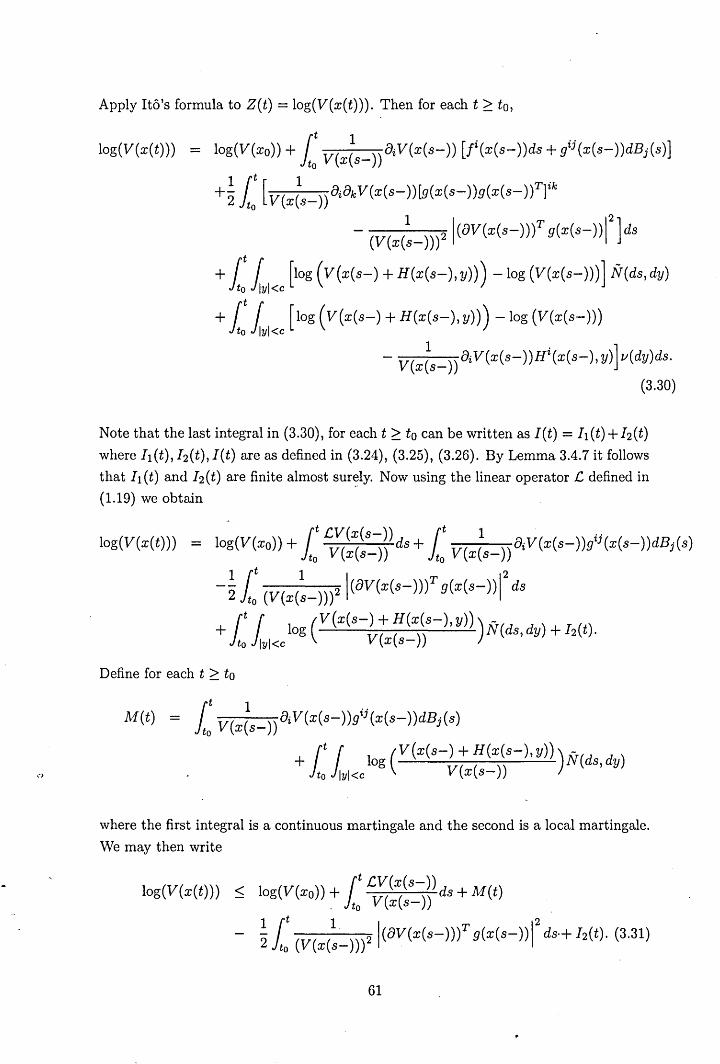
Apply Ito's formula to Z(t) = log(V(x(t))). Then for each t ~ to,

log(V(x(t))) = log(V(xo)) + 1: V(x~s-)) 8i V(x(s-)) [i(x(s-) )ds + gij (x(s- ))dBj(s)]

1 (t [ 1 T]ik +2 ito V(x(s- )) OiOk V(x(s-)) [g(x(s-) )g(x(s-))

_ 1 21(oV(x(s-)))T g(x(s-))12

]dS (V(x(s- )))

+ t r [log (V(x(s-) + H(x(s-),y))) -log (V(x(s-))) 1 N(ds,dy) ito i1yl<c

+ r r [log (V(x(s-) +H(x(s-),y))) -log (V(x(s-))) ito i1yl<c

1 .] - V(x(s- )) Oi V(x(s- ))Ht(x(s-), y) v(dy)ds.

(3.30)

Note that the last integral in (3.30), for each t ~ to can be written as I(t) = It (t) + I2(t)

where It(t), I2(t), I(t) are as defined in (3.24), (3.25), (3.26). By Lemma 3.4.7 it follows

that II (t) and I 2(t) are finite almost sur~ly. Now using the linear operator C defined in

(1.19) we obtain

(t CV(x(s-)) (t 1 .. log(V(x(t))) = log(V(xo)) + ito V(x(s-)) ds + ito V(x(s-)) oiV(x(s-))lJ(x(s-))dBj(s)

1 {t 1 1 12 -2" ito (V(x(s- )))2 (8V(x(s- )))T g(x(s-)) ds

{t ( (V(x(s-) + H(X(S-),y))) _ + ito i1yl<c log V(x(s- )) N(ds, dy) + I2(t).

Define for each t ~ to

(t 1 " M(t) = ito V(x(s- )) 8i V(x(s- ))lJ (x(s- ))dBj(s)

+ {t ( log (V(x(s-) + H(X(S-)'Y)))N(ds,dY) ito i1yl<c V(x(s-))

where the first integral is a continuous martingale and the second is a local martingale.

We may then write

(t CV(x(s-)) log(V(x(t))) < log(V(xo)) ~ ito V(x(s- )) ds + M(t)

-21 (t 1 21(oV(x(s-)))T g(x(s_))1

2 ds.+ I2(t). (3.31) ito (V(x(s- )))

61

We now use the exponential martingale inequality (3.9) for T = n, Q = e and (3 = en

where e E (0,1) and n E N. Then for every integer n ~ to, we find that

p[ sup {M(t) -:'2 (t 1 21(8V(x(s-)))T g(x(s_))12

ds to~t~n lto (V(x(s-)))

1 it 1 [ (V :c(s- )+H(:c(s- ),y) ) e

log V(:c s- ) -- e -1

£ 0 Ixl<c

_ 1 (V(X(S-) + H(x(s-), y)))] (d)d} > ] < -c2n £ og V(x(s-)) lJ Y s en _ e .

Since 2:~=1 e-c2n < 00 then an application of the Borel-Cantelli lemma and elementary

probability calculations, as in the proof of Theorem 3.4.1, yields. that

p[liminf { sup (M(t) - -2£ {t 1 21(8V(x(s-)))T g(x(s_))12

ds n-oo to:5t:5n lto (V(x(s- )))

_ ~ (t 1 (V(X(S-) + H(X(S-)'Y)))C -1 e lo Ixl<c V(x(s-))

( V (x (s- ) +H (x (s - ), y) ) ) ) }]

~ e log V(x(s-)) v(dy)ds ::; en = 1.

Hence for almost all wEn there is a random integer no = no(w) such that for n ;:::: no, to ::; t ::; n,

M(t) < ~ 1: (V(x(~-)))21 (8V(x(s-))f g(x(s-)) 12 ds + en

+~ {t r [(V(X(S-)+H(X(S-),y)))C_ 1 £ lto llyl<c V(x(s-))

_ 1 (V(X(S-) + H(X(S-),y)))] (d)d (3.32) £ og V(x(s-)) lJ Y s.

Substituting (3.32) into (3.31) and using conditions (ii) and (iii) it follows immediately

62

that

log(V(x(t))) 1

::; log(V(xo)) - 2" [(1 - c )C3 - 2C2] (t - to) + en

+it r [lOg (V(X(S-)+H(X(S-),y))) +1- V(X(S-)+H(X(S-),y)))] v(dy)ds to J1yl<c V(x(s-)) V(x(s-))

+~ it r [ (V(x(s-) + H(x(s-), y)))c _ 1 c to J1yl<c V(x(s-)) ,

_ 1 (V(X(S-) + H(X(S-),y)))] (d)d (3.33) c og V(x(s-)) v y S

for n 2:: no, to :5 t :5 n.

Fix x E JRd and define for y E B h (y) = 11 (V(X+H(X,y)))C -1- clog (V x+H(x,y )) I. c, c c V(x) V x

We easily deduce that (V(X+H(X,y)))C - 1 - clog (V(X+H(X,y))) > 0 for all y E B by V(x) V(x) - c,

using the elementary inequality eb - 1 - b ~ 0 for b E JR. Since c E (0,1) then we can

use the inequality bC < 1 + c(b - 1) for 0 < c < 1 and b > 0 (see Hardy, Littlewood and

P6lya [17] pp. 40) to deduce that for ally E Bc ,

Note that by Lemma 3.4.7 (iii) the right hand side of (3.34) is Lebesgue integrable and

is v-integrable on Bc. It follows that the same applies for hc(Y).

Now let c ~ O.

The dominated convergence theorem yields that for all t 2:: to

limit r ~[(V(X(S-)+H(X(S-),Y)))C_1 c-o to J1yl<c c V(x(s-))

_ 1 (V(X(S-) + H(X(S-),y)))] (d)d c og V (x ( S _ ) ) ~ v y S

= it r lim ~ [(V(X(s-) +H(X(S-),y)))C -1] to J1yl<c c-o c V(x(s-))

-1 (V(X(S-) + H(X(S-),y))) (d)d og V(x(s-)) v y S

= o. (3.35)

63

Hence by (3.35) for n ~ no, to ::; t ::; n, (3.33) becomes

log(V(x(t))) ::; 1

log(V(xo)) - "2 (C3 - 2C2) (t - to)

ltl [ (V(X(S-)+H(X(S-),y))) + log + 1 to Iyl<c V(x(s-))

_ V(x(s-) + H(X(S-),y))] (d)d V(x(s-)) v y s. (3.36)

Now substituting condition (iv) into (3.36), we see that for almost all wEn,

to + n - 1 ::; t ::; to + n, n ~ no

1 I (V( (t))) < t - to ( 2) log(V(x( to))) t - to - og x --- C3 - C2 + - --C4· t - 2t to + n - 1 t

Now applying condition (i) we obtain that

lim sup ~ log Ix(t)1 < t-+oo t

a.s.

o

3.5 Moment exponential stability

The main aim of this section is to introduce criteria for the solution of an SDE driven

by a Levy process to be moment exponentially stable and to derive a relation between

moment and almost sure exponential stability.

The following result is an extension of Mao's work [33] Chapter 4, Theorem 4.4 pp. 130.

Theorem 3.5.1 Let p, 01, 02, 03 be positive constants. If V E C2(JRd j JR+) satisfies

(i) ollxlP ::; V(x) ::; 021x1P ,

(ii) .cV(x) ::; --03V(X),

for all x E lRd, then

for all t 2: to (3.37)

for all Xo E JRd. As a result the trivial solution of (3.1) is pth moment exponentially

stable under conditions (i) and (ii) and the pth moment Lyapunov exponent should not

be greater than -03'

64

Proof: Fix any xo i= 0 on JRd. For each n ~ Ixol define the stopping time

Tn = inf {t ~ to : I x ( t) I ~ n}

so that, Tn i 00 almost surely.

Apply Ito's formula to Z(t) = exp(a3(t - to))V(x(t)). Then, for each t ~ to,

exp(Q3(t 1\ Tn - to))V(x(t 1\ Tn))

ltl\Tn

= V(XO) + Q3 exp(Q3(S - to))V(x(S~ ))ds to

ltl\Tn

+ exp(a3(s - to) )8i V(x(s-)) [fi(x(s- ))ds + gij (x(s- ))dBj(s)] to

I1tl\Tn + '2 exp(a3(s - to))8i8k V(x(s- ))[g(x(s-))g(x(s- ))T]ikds to

+ ltMn ( exp(0'3(S - to)) [V(x(s-) + H(x(s-), y)) - V(x(s-))] N(ds, dy) to J1yl<c

l tl\Tn 1 [ + exp(Q3(S - to)) V(x(s-) + H(x(s-),y)) - V(x(s-)) to Iyl<c

- 8i V(x(s...;;. ))Hi(x(s-), y)] v(dy)ds.

Hence

[ ltl\Tn

E[ exp(Q3(t 1\ Tn - to))V(x(t 1\ Tn))] = V(xo) + E exp(Q3(S - to)) [Q3V(X(S-)) to

+CV(x(s-))]ds]. (3.38)

Now, apply condition (ii) within (3.38) to obtain

E[ exp(Q3(t 1\ Tn - to))V(x(t 1\ Tn))] ~ V(XO). (3.39)

From condition (i) (left hand inequality), we have

Taking expectations and using (3.39) and then applying condition (i) again (right-hand

inequality), it follows that

QIE [lx(t 1\ Tn)IP exp(Q3(t 1\ Tn - to))] < E[V(x(t 1\ Tn)) exp(Q3(t 1\ Tn - to))]

< V(XO) ~ Q21xo1P. (3.40)

65

Hence,

which implies that

U sing the fact that for each t ~ to, 1 [0,7" n] exp (Q3 (t - to)) I x ( t) IP forms a monotonic

increasing sequence of random variables then by the monotone convergence theorem it

can be deduced that

And the result follows. o

Proposition 3.5.2 If the trivial solution of (3.1) is pth moment exponentially stable

then the trivial solution is qth moment exponentially stable for every q < p.

Proof: Let q < p. An application of Holder's inequality yields that

(3.41)

Since the trivial solution of (3.1) is pth Inoment exponentially stable using (1.23) and

(3.41) then,

E [lx(t)IQl < [ClxolP exp (->.(t - to)) 1 ~ = dlxolq exp ( - Cq) (t - to)) .

Hence,

~

where D = C~ > 0 and>..' = ~ > 0 which means that the solu~ion is qth moment

exponentially stable. 0

It is very interesting to mention that in general there is no obvious relation between

exponential and almost sure stability. Kozin in [24] pp. 107 refers to an example of

an SDE driven by a Brownian motion where the system is almost surely stable but is

not moment exponentially stable. However it is possible when moment .stability holds

to deduce almost sure stability under some additional conditions. Mao in [33] Theorem

66

4.2, Chapter 4 pp. 128 establishes such a relation. In the following we will generalize

Mao's result and give the relationship between the pth moment exponential stability

and almost sure exponential stability for the trivial solution of (3.1).

We will need to use among others, two inequalities: the Burkholder-Davis-Gundy (BDG)

inequality and Kunita's estimate for a compensated Poisson integral. For the sake of

completeness we state the BDG inequality here.

Theorem 3.5.3 (Burkholder-Davis-Gundy inequality)

Let b E P2 (T). Define for t ;::: to

x(t) = rt b(s)dB(s) ito

and A( t) = rt IIb( s) 112ds.

ito

Then for every k > 0 there exist universal positive constants Ck, Ck, such that

for all t ;::: to. In particular we may take the following choices

Proof: See Mao [33] pp. 40.

if 0 < k < 2,

if k = 2,

if k> 2.

o

Now we need to discuss Kunita's estimate in a little more detail for reasons that

will become obvious below. For the purposes of the following proof let Y(t) = t -

Ito ~YI<c H(x(s-), y)N(ds, dy). Applying Ito's formula to the process IY(t)IP for each t ;::: to, we have

IY(t)l1' = rt r {IY(s-) + H(x(s-), y)IP - IY(s-) IP }N( ds, dy) ito i1yl<c

+ t r {IY(s-) + H(x(s-), y)!P -IY(s-)!P ito i1yl<c

- pIY(s_)IP-2Y(s_)T H(x(s-), y) }v(dy)ds, (3.42)

where the first term in (3.42) is a loc.al martingale.

t -For p ;::: 2 and Y(t) = Ito ~YI<c H(x(s-), y)N(ds, dy) and letting f = 0 and g = 0 then

67

.;>

Kunita's estimate (Theorem 3.2.1) becomes .

E [ sup IY(s)IP] ::; to~s~t

c7(p)E [(it f IH(x(s-), Y)12V(dY)dS)~] to J1yl<c

+cs(p)E [(it f IH(x(s-), Y)IPV(dY)dS)] to J1yl<c

where C1(p) and cs(p) are positive constants that depend only on p.

For a proof see Kunita [25] pp. 334.

(3.43)

Remark 3.5.4 Recall that in the context of stability theory we are always assuming

that f(O) = 0 and g(O) = 0, hence from the Lipschitz conditions on the drift and

diffusion coefficients we deduce that for all x E ]Rd there exists L > 0 such that

If(x)1 ::; VLlxl and

Hence,

where L' = max{ VI, L} and this will be used in the proof of the theorem below.

Theorem 3.5.5 Assume that assumption 3.2.2 holds. For p 2:: 2, pth moment

exponential stability, of the trivial solution to (3.1), implies almost sure exponential

stability.

Proof: Fix any Xo =I- 0 on ]Rd. If the solution is pth moment exponentially stable then

on t 2:: to (3.45)

with A and 0' positive constants .

Let n E N. Apply Ito's formula to Z(t) = Ix(t)IP. For to + n - 1 ::; t ::; to + n the

68

following holds almost surely

Ix(t)IP = Ix(to + n - l)IP + {t plx(s- )IP- 2x(s-)T f(x(s- ))ds Jto+n-l

+ ~ rt (plx(s- )IP-21Ig(x(s-)) 112 + p(p - 2) Ix(s- )IP-4Ix(s-)T g(X(S- ))12) ds 2 Jto+n-l

+ rt plx(s- )IP-2x(s-)T g(x(s- ))dB(s) Jto+n-l

+ t r (Ix(s-) + H(x(s-), y)IP"': Ix(s-)IV )N(ds, dy) Jto+n-l J1yl<c

+ {t ((Ix(s-) + H(x(s-),y)IP -Ix(s-)IP Jto+n-l J1yl<c

- plx(s- )IP-2x(s-)T H(x(s-), y)) v(dy)ds.

Applying (3.44) then,

Ix(t)IP < Ix(to+n-1)IP+ C1 {t Ix(s-)IPds Jto+n-l

+ (t plx(s-)IP- 2x(s-)Tg(x(s-))dB(s) Jto+n-l

+ rt· r (Ix(s-) + H(x(s-), y)IP -Ix(s-)IP )N(ds, dy)

Jto+n-l J1yl<c

+ rt 1. (Ix(s-) + H(x(s-), y)IP -Ix(s- )IP Jto+n-l Iyl<c

- plx(s-) IP- 2x(s-)T H(x(s-), y)) v(dy)ds

L' where Cl = pL' + 1!f [1 + (p - 2)]. Hence,

E [to+n-~~~::;to+n Ix(t)IV]

lto+n

::; E [Ix(to + n - 1) IP] + Cl E [Ix(s-) IP] ds . to+n-l

+ E [ sup (t plx(s-) IP-2 x(s-)T g(x(s- ))dB(S)] to+n-l$t$to+n Jto+n-l

+ E [ sup {t r (I~(s-) + H(x(s-), y)IP - Ix(s-)lV) N(ds, dy) to+n-l~t$to+n Jto+n-l J1yl<c

+ t r (Ix(s-) + H(x(s-), y)IP -Ix(s-)IP Jto+n-l J1yl<c .

- plx(s- )IP-2x(s-f H(x(s-), y) )V(dY)dS}]. (3.46)

For the Brownian motion integral, by the Burkholder-Oavis-Gundy inequality with

69

b(t) =plx(t-)IP-2x(t-)Tg(x(t-)) and k = 1 thEm (see Mao [33] pp. 129)

E [ sup it plx(s- )IP- 2x(s-)T g(x(s- ))dB(S)] to+n-15t5to+n to+n-l

:::; ~E [ sup Ix(t-)IP] + 16p2L'lto+n E[lx(s-)IP]ds. 2 to+n-15t5to+n to+n-l

(3.47)

Define

h = E[ sup {it r (Ix(s-) + H(x(s-),y)IP -lx(s-)lP)N(ds,dy) to+n-15t5to+n to+n-l J1yl<c

+ it f (Ix(s-) + H(x(s-), y)IP -Ix(s- )IP to+n-l J1yl <c

- plx(s- )IP-2x(s-)T H(x(s-), y)) V(dY)dS}].

Since the integrals have the same form as in (3.42), applying Kunita's estimate (3.43)

it follows that

h :::; c7(p)E [(lto

+n

f IH(~'(s-), Y)12l/(dY)dS)~] to+n-l J1yl<c

+ cs(p)E [(lto

+n

f IH(x(s-), Y)IPl/(dY)dS)] . (3.48) to+n-l J1yl<c

An application of Holder's inequality to the first term on the right-hand side of (3.48)

yields

h < C7(p, t)E [lto

+n (f IH(x(s-), Y)1 2l/(dY)) ~ dS]

to+n-l J1yl<c

+ cs(p)E [(lto

+n

f IH(x(s-), Y)IPl/(dY)dS)]. (3.49) to+n-l J1yl<c

o Using assumption 3.2.2 within (3.49), we obtain

h :::; C7(p, t)E [lto

+n

(Klx(s- )12) ~ dS] .+ cs(p)E [lto

+n

Klx(s- )IPdS] to+n-l to+n-l

= Cp(t)E [lto

+n

Ix(s- )IPdS] (3.50) to+n-l

70

E . where Op(t) = C7(p, t)K 2 + c8(p)K. By (3.47) and (3.50) then (3.46) becomes

E [ sup Ix(t)IP] :::; E[lx(to + n - 1)IP] + -21 E [ sup Ix(t- )IP]

to+n-l$t$to+n to+n-l$t$to+n

+(Cl + 16p2 L' + Op(t)) ({to+n E[lx(s)IP]dS). (3.51) lto+n-l

Rearranging, for p ~ 2

[ ] lto+n

E sup Ix(t)IP:::; 2E[lx(to + n - 1)IP] + 0 E[lx(s)IP]ds to+n-l$t$to+n to+n-l

(3.52)

where C is a positive constant depending on p, t, K and L'.

Define Ll = E[lx(to + n - 1)IP]. Since the solution is pth moment exponentially stable,

then by (3.45)

Define

lto+n

L2 = E[lx(r)IP]dr. to+n-l

Again using (3.45) and integrating, we see that

lto+n I IP

L2 = E[lx(r)IP]dr < 0' x~ (e->.(n-l) _ e->.n) to+n-l 1\

<_ c,lxo\P ->.(n-l) ,\ e .

Hence,

E [ sup Ix(s)IP] < {2Ll + OL2} = 03e->.(n-l) (3.53) to+n-l$s$to+n

where 0 3 = Ixo1P(20' + cf'). Now we argue as in Mao [33] pp. 129-130 and the required result follows. o

In applications Lyapunov functions are often taken to be quadratic functions of the form

(3.54)

where Q is a symmetric positive definite matrix.

In the following corollary we will give some explicit conditions on the coefficients of (3.1)

71

using a Lyapunov function based on (3.54), in order to prove that the trivial solution of

(3.1) is pth moment exponentially stable for p > O. This is a generalization of Corollary

4.6, Chapter 4 pp. 131-132 in Mao [33].

For completeness, we first provide a proof of the following well-known result, that will

be used in the corollary below and in other parts of this thesis.

Proposition 3.5.6 If D is a d x d real-valued symmetric matrix then for all x =1= 0

(3.55)

where J..Li, 1 ~ i ~ d are the eigenvalues of the matrix D.

Proof: If D is a d x d symmetric matrix then it has real eigenvalues J..LI, ... ,J..Ld and there

exists an orthogonal matrix 0 such that OT DO = diag(J..LI, ... , J..Ld). Hence,

where Xl = OT X

Hence,

~d J..L.(xi )2 min{II..} < L.Ji=1 t I < max{II..}

,.-t - ~d (i)2 - ,.-~ L.Ji=1 Xl

and the required result follows. o

Corollary 3.5.7 Assume that for all X E lRd ~YI<c IxTQH(x,y)lv(dy) < 00 and the following assumptions hold:

(i) xTQf(x) + ~tr (gT(x)Qg(x)) - r xTQH(x,y)v(dy) ~ blxTQX, . J1yl<c

(ii) b2xTQx ~ IxTQg(x) I ~ b3xTQx, "

(iii) r [((x + H(x, y))TQ(x + H(x, y)) ~.- (xTQx) ~ v(dy)] ~ b4P(xTQx)~, J1yl<c

where Q is a symmetric positive-definite d x d matrix and bl to b4 are constants.

(a) If bl < 0 and b4 < 0 then the solution to (3.1) is pth moment exponentially stable

if it holds that p < 2 + 21b l l/b32 + 2Ib41/b~.

(b) If bl ~ 0, b4 ~ 0 such that 0 ~ bl + b4 < b~ then the trivial solution of {3.1) is pth

moment exponentially stable if it holds that p < 2 - 2bl /b22 - 2b4/b2

2 •

72

Proof: Since Q is a symmetric positive-definite matrix it has real positive eigenvalues

AI, ... ,Ad' Define Amin and Amax to be the smallest and largest eigenvalues of Q

respectively. Then by proposition 3.5.6 we see that for x =f 0

and for p ~ 2, we have that

Define V(x) = (xTQx)~. Hence,

where bl, b2 are positive constants and we can see that condition (i) from Theorem 3.5.1

is satisfied.

Now the linear operator £, as given by (1.19) applied to the function V yields

£'V(x) = p(xTQx)(~-l)(xTQf(x) + ~tr(gT(x)Qg(x)) + p (~-1) (xTQx)(~-2)lxTQg(x)12

+ r [((X+H(X,y))TQ(X+H(X'Y)))~ - (xTQx)~ J1yl<c

- p(xTQx)(~-l)xTQH(x, y)] lI(dy).

Hence,

£'V(x) = p(xTQx/~-l) (xTQf(X) + ~tr(gT(x)Qg(x)) - r XTQH(X,Y)V(dY)) 2 J1yl<c

+ p (~ -1) (xTQx/~-2)lxTQg(x)12 + r . [((x+H(x,y))TQ(X+H(x,y))~_(xTQx)~]v(dy).

J1yl<c .

Case 1: bl < 0, b4 < ° and p < 2 + 2Ibll/b~ + 2Ib41/b~ This implies that Ibll- (~ - 1) b32 + Ib41 > 0. Applying conditions (i) to (iii) then,

£'V(x) < -p [Ibll- (~ - 1) b32 + Ib41] V(x)

i.e. £'V(x) < -C3 V(x)

where C3 = P [Ibll- (~ - 1) b32 + Ib41] is a positive constant.

73

We see that under these assumptions condition (ii) of Theorem 3.5.1 is satisfied, and it

follows that the trivial solution of (3.1) is pth moment exponentially stable.

Case 2: bl ~ 0, b4 ~ 0 such that 0 ~ b1 + b4 < b~ and p < 2 - 2bl/b~ - 2b4/b~. Again applying conditions (i) to (iii) then,

.cV(x) ::; -p [-b1 - (~- 1) b22

- b4] Vex)

i.e. .cV(x)::; -C4 Vex)

where C4 = P [-bl - (~ - 1) b22

- b4] is a positive constant.

Since the conditions of Theorem 3.5.1 are satisfied then again the trivial solution of

(3.1) is pth moment exponentially stable. 0

74

<}

Chapter 4

Stochastic Stabilization and

Destabilization

4.1 Introduction

Assume that we have the system of non-linear ordinary differential equations

dx(t) = f(x(t)) dt

on t 2:: to (4.1)

Assumption 4.1.1 We assume that f : lRd -+ lRd is a locally Lipschitz continuous

function and furthermore, for some K > 0

If(x)1 :::; Klxl for all x E lRd, (4.2)

e.g. f(x) = xe-x2 for x E lRd or f(x) = 1 - e-x for x > O.

We require that t~is assumption holds for the rest of this chapter.

Now suppose that the non-linear system (4.1) ~s perturbed by random noise and

therefore a stochastic system is created. It is possible when a system is perturbed

by noise that it can be stabilized if it is unstable, in the sense that by adding noise we

can force the solution of the stochastic differential equation to converge to the trivial

solution as time- increases indefinitely. This is the goal of stochastic stabilization. On

the other hand, a system can be destabilized when perturbed by noise, in th~ case that

the unperturbed system is stable. In this instance, by adding noise the sample paths of

the process escape to infinity (a.s.) instead of converging to the trivial solution as time

75

<>

increases indefinitely.

These ideas of stabilization have evolved through the work of Bellman [6] and Merkov

[36] who used deterministic periodic noise to stabilize a system. Pioneering work on

stochastic stabilization has been carried out by Khasminski and Arnold in [22] and [5]

respectively. Khasminski has used two independent white noises to stabilize a system

and Arnold has shown that a linear ODE system of the form dx(t) = Ax(t)dt can be

stabilized by a zero mean stationary noise if and only if tT A < O. Mao in [31] and [33]

pp. 135-141 uses an m-dimensional Brownian motion process B = (B(t), t ~ 0), where

for each t ~ 0 B(t) = (Bl(t), ... , Bm(t)), as the source of noise to perturb the given

system (4.1) and he establishes a general theory of stochastic stabilization for the given

non-linear system. The perturbed system has the form:

m

dx(t) = f(x(t))dt + L Gkx(t)dBk(t) on t ~ 0 (4.3) k=l

where Gk E Md(]R), for 1 :5 k :5 m, and initial condition x(O) = Xo E ]Rd.

Motivated by Mao's theory (see Mao [31] and,[33] pp. 135-141) we would like to extend

his results and investigate conditions under which the given non-linear system (4.1) can

be stabilized or destabilized, if it is perturbed by a more general noise. The main purpose

of this chapter is to examine sufficient criteria for stability of non-linear deterministic

systems when they are perturbed by Levy-type stochastic integral terms. In fact we

will examine almost sure exponential stability.

Although moment exponential stability is stronger than almost sure exponential stability

(see Chapter 3, Theorem 3.5.5); as shown by Kozin [24] pp. 107 and Mao [33] it is

possible for the stochastically perturbed system to have unbounded moments but to be

almost surely exponentially stable. Hence for examining stabilization is better to avoid

moment properties and aim to stabilize (4.1) in an almost sure exponential way.

In the following we will give the proper mathematical set up for this chapter.

Assume that we are given an m-dimensional standard Ft-adapted Brownian motion

process B = (B(t), t ~ 0) with B(t) = (B1(t), ... , Bm(t)) for each t ~ 0 and an

independent Ft-adapted Poisson random measure N defined on ]R+ x (]Rm \ {O}) with

compensator IV ~f the form N(dt, dy) = N(dt, dy) -"- v(dy)dt where v is a Levy measure.

In this chapter the stochastically perturbed system corresponding to (4.1) will have the

following form

dx(t) = f(x(t- ))dt + f GkX(t~ )dBk(t) + r D(y)x(t- )N(dt, dV) k=l J1yl<c

76

+ r E(y)x(t-)N(dt,dy) (4.4) JIYI~c

for all t ~ to, where Gk E Md(lR), for 1 :::; k :::; m, and D and E are suitable matrix

valued functions.

Given the initial condition x(to) = Xo E jRd, the uniqueness and existence of the solution

of the SDE (4.4) when 1 : jRd -+ jRd is a locally Lipschitz continuous function, is

guaranteed from Theorem 4.2.1 that will be proved in the sequel (see section 4.2). The

unique solution to (4.4) is denoted by x(t) for each t ;::: to. For all x E jRd define

g(x) = 2:~=1 GkX , H(x, y) = D(y)x for Iyl < c and K(x, y) = E(y)x for Iyl ~ c. Assume that 1(0) = 0, then (4.4) has a solution x(t) = 0 for all t ~ to corresponding to

the initial value x(to) = 0, which is the trivial solution.

This chapter will be organized as follows:

In section 4.2 we will give the proof for the existence and uniqueness of solutions for

Levy driven SDEs with locally Lipschitz coefficients under some additional conditions.

In section 4.3 we will describe some of the mathematical tools needed to develop the

analysis in this chapter. In the other sections we turn our attention to the stabilizing

effects of the noise when it is added to the deterministic system (4.1). Our aim in the

later sections is to find conditions under which the Lyapunov exponent is negative so

that the solution of the stochastically perturbed system of the non-linear deterministic

system is almost sure exponentially stable. In order to make our discussion simple we

will examine separately the perturbation of (4.1) first by small jumps (by a compensated

Poisson integral) and then by large jumps (by a Poisson integral), in sections 4.4 and

4.5 respectively. In section 4.6 we will combine the results of sections 4.4 and 4.5 in

order to have conditions for almost sure exponential stability for the trivial solution of

the stochastically perturbed system driven by a Levy process. In sections 4.7 and 4.8

we will consider some special cases of the theory that was developed in the previous

sections. In section 4.7 we will examine the stabilization of a one-dimensional linear

deterministic system perturbed by a Brownian motion and a single Poisson process.

Finally, in section 4.8 we focus on the stabilization of a non-linear system perturbed

with Brownian motion and a compensated Poisson process and on the destabilization

of a stable SDE driven by Poisson noise perturbed with Brownian motion.

4.2 Existence and uniqueness t~eorem for Levy driven

SDEs with locally Lipschitz coefficients

Since f : lRd -+ ]Rd is a locally Lipschitz continuous function and not necessarily Lipschitz

continuous it is not possible to apply Theorem 1.4.1 (i). In the following we will prove

the existence of a unique solution to SDEs driven by a Levy process when the coefficients

satisfy local Lipschitz conditions and the growth conditions (C2).

77

Consider the following general d-dimensional SDE

dx(t) = j(x(t- ))dt + g(x(t- ))dB(t) + r H(x(t-), y)N(dt, dy) (4.5) J1yl<c

on to ~ t ~ T with initial value x(to) = Xo, such that Xo E JRd.

For the rest of this section we impose the following conditions on the coefficients of

(4.5).

Assume that the growth conditions (C2) as defined in Chapter 1 hold and

Local Lipschitz conditions: For every n ~ 1 there exists a positive integer Kn such

that for all Xl, X2 E JRd with IXII V IX21 ~ n

(4.7)

In Applebaum [1] Theorer.n 6.2.11 pp. 313 it has been proved that under local Lipschitz

and local growth conditions on the coefficients of (4.5) there exists a unique local

solution. As we will show in the sequel under the local Lipschitz conditions and the

global growth conditions (C2) we can prove that their exists a global solution to (4.5).

The following is a generalization of Mao's work [33] pp. 57, that deals with the case

H=O.

Theorem 4.2.1 Assume that the local Lipschitz conditions (4.6), (4.7) and linear

growth conditions (C2) hold. Under these conditions then (4.5) has a unique cddldg,

adapted solution for all t E [to, T].

Before we prove Theorem 4.2.1 we need to prepare a lemma .

.;> For n ~ 1 define

if Ixl ~ n

if Ixl > n

if Ixl ~ n

if Ixl > n

{H(X' y) if Ixl ~ n, Iyl < c

Hn(x,y) = ( ) H [xf,y if Ixl > n, Iyl < c

(4.8)

(4.9)

(4.10)

where j, 9 and H satisfy the local Lipschitz conditions (4.6) and (4.7), and the growth

78

conditions (C2).

Lemma 4.2.2 Let in,gn, Hn be defined as in (4.8), (4.9) and (4.10) respectively.

Then in, gn and Hn satisfy the global Lipschitz conditions (C1).

Proof: As 1¥x71 = n for all Xi E ]Rd, i = 1,2, when \XI\, \X2\ > n we have

with Kn > O. Then by (4.11) we have that

Hence,

Now for \XI\, \X2\ :5 n the local Lipschitz constant is Kn.

For \XI\ > nand \X2\ :5 n we have

By (4.12) it follows that

79

( 4.12)

and this implies that

The same arguments applies for IX21 > nand IXII ~ n.

The arguments for 9n and Hn are similar in all cases.

Hence with this truncation procedure we have shown that for all Xl, X2 E ]Rd, fn,9n, Hn

satisfy the global Lipschitz conditions (C1) with Lipschitz constant L = Kn. 0

Now we are ready to proceed with the proof of Theorem 4.2.1.

Proof of existence: Define for n ;:::: 1

Xn(t) = Xo + it fn(xn(s- ))ds + it 9n(Xn(S- ))dB(s) + it r Hn(xn(s-), y)N(ds, dy) to to to J1yl <c

where fn, 9n, Hn satisfy (4.8), (4.9) and (4.10) respectively. Then by Lemma 4.2.2 fn,

9n and Hn satisfy the glob.al Lipschitz conditions (C1) with Lipschitz constants L = K n, and the growth conditions (C2). Hence, by Theorem 1.4.1 (i) for all t E [to, T] there

exists a unique solution to (4.13).

N ow define the stopping times

an = inf {t E [to, T] : IXn(t)1 ~ n} and Tn = T 1\ an. (4.14)

We claim that for n ~ 1

Xn(t) = Xn+l(t) (a.s.) if to ~ t ~ Tn. (4.15)

For to ~ t ~ Tn, we have IXn(t)1 ~ n (a.s.). By (4.8) it follows that fn(xn(t)) = f(xn(t))

(a.s.). Also since l:J;n(t) I ~ n < n + 1, then fn+l(Xn(t)) = f(xn(t)) (a.s.). Hence,

(4.16)

The same applies for the diffusion and jump coefficient.

. Hence for to ~ t ~ Tn by (4.16) we have that with probability 1

80

(4.13)

= rt [fn+l(Xn+l(S-)) - fn(xn(s- ))] ds + rt [9n+l(Xn+l(S-)) - 9n(Xn(S- ))] dB(s) lto lto

+ rt r [Hn+l(Xn+l(S-), y) - Hn(xn(s-), y)] N(ds, dy) lto llyl<c

= rt [fn+l(Xn+l(S-)) - fn+l(Xn(S- ))] ds + rt [9n+l(Xn+l(S-)) - 9n+l(Xn(S- ))] dB(s) lto lto

+ rt r [Hn+l(Xn+l(S-),y) - Hn+l(Xn(S-),y)]N(ds,dy). (4.17) lto llyl<c

Using (1.12), with n = 3, taking expectations, then using standard arguments (see e.g.

Applebaum [1] pp. 306-307) and applying the global Lipschitz conditions (C1) with

L = Kn we see that

where en > O.

Now applying Gronwall's inequality we get

Hence the claim (4.15) is verified.

Now, since (4.15) holds for to ::; t ::; Tn, we have that

Tn = T /\ inf {t E [to, T] : IXn+l(t)1 ~ n}

< T /\ inf {t E [to, T] : \Xn+l(t)\ ~ n + I}

(4.18)

Hence, ( Tn, n E N) .is an increasing sequence.

For t E [to, T], then

Xn(t /\ Tn) = Xo + rt fn(xn(s- ))l[to,Tn]ds + rt 9n(Xn(S-))1[to,Tn]dB(s) lto lto

+ rt r Hn(xn(s-), y)l[to,Tn]N(ds, dy). (4.19) lto llyl<c

Using (1.12), with n = 4, and following standard arguments (see e.g. Applebaum [1]

81

pp. 306) we can see that

4 (1 + Ixol2) + 4(T - to) it E [ Ifn(Xn(S- ))1[to'TnJi2

] ds to

+161t

E [19n(Xn(S- ))1[to,Tnl n ds to

+161t r E [!Hn(xn(s-), y)1[to,Tnl 12] v(dy)ds. to J1yl<c

( 4.20)

Now applying the growth conditions (C2) and Gronwall's inequality, there exists K' > 0

such that

E [sup IXn(s 1\ Tn)1 2] ~ E [sup (1 + IXn(s 1\ Tn)12)] ~ 4(1 + IxoI2)e4K'(T-to) to'5.s'5.t to'5.s'5.t

(4.21)

By Chebyshev's inequality and (4.21), for n 2:,,1 we obtain that

( ) E [SUPto'5.s'5.t IXn(s 1\ Tn)12] 4(1 + IxoI)2e4~'(T-to)

p sup IXn(sI\ Tn)l2: n ~ 2 ~ 2 • to'5.s'5.t n n

Since 2:~=1 ~ < 00 we can apply the Borel-Cantelli Lemma to deduce that for almost

all wEn there is a random integer no = no(w) E N such that for n 2: no(w)

P (liminf sup IXn(s 1\ Tn)1 < n) = 1. n-H)Q to '5.s '5.t

Hence for n 2:: no(w), IXn(t 1\ Tn)1 < n a.s.

Assume that an --+ To < T as n --+ 00 (a.s.). Then it follows that there exists an integer

rno E N such that IXm(t 1\ Tn)1 2:: rn for all rn 2:: rno and this yields a contradiction.

Hence we can deduce that for an --+ 00 (a.s.) and Tn --+ T (a.s.) as n --+ 00.

Now define x'(t) = xno(t) for t E, [to, T]. "

For n 2:: no, applying (4.15) repeatedly yields that xno(t 1\ Tn) = xn(t 1\ Tn). Hence,

x'(t 1\ Tn) = xn(t 1\ Tn). Then (4.13) becomes

1

tl\Tn 1tl\Tn x'(t 1\ Tn) = Xo + fn(x'(s-))ds + gn(x'(s-))dB(s)

to to

+ ltl\Tn r . Hn(x'(s-), y)N(ds, dy). (4.22) to J1yl<c

Since for n 2:: no, Ix'(t 1\ Tn)1 ~ n then by (4.8), (4.9) and (4.10), (4.22) can be written

82

as

itATn itATn

x'(t /\ Tn) = Xo + f(x'(s- ))ds + g(x'(s- ))dB(s) to to

ltATn

1 + H(x'(s-), y)N(ds, dy). to Iyl<c

Let n --+ 00. Since limn_co Tn = T (a.s.) then

x'(t) = Xo + it f(x'(s-))ds + it g(x'(s-))dB(s) + it ( H(x'(s-),y)N(ds,dy). to to to J1yl <c

Hence, we see that x'(t) is a solution to (4.5).

Proof of uniqueness: Let (x(t), t E [to, T]) and (y(t), t E [to, T]) be two distinct global

solutions of (4.5). Let (Tn, n E N) be as defined in (4.14). Since x and yare both local

solutions for all to :5 t :5 Tn then by uniqueness of local solutions (see Applebaum [1]

Theorem 6.2.11 pp. 313) we have that x(t) = y(t) (a.s.) for all to :5 t :5 Tn. Then by

the continuity of probability we obtain

P (x(t) = y(t) for all t E· [to, T]) = P (n (x{t) = y{t) for all to ~ t ~ Tn») = 1, nEN

as required. o

Remark 4.2.3 If the assumptions (4.6) and (4.7) hold on every finite subinterval [to, T] of [to,oo), along with the growth conditions (C2), then we will have a unique global

solution on [to, 00) (see e.g. Mao [33] pp. 58).

We also remark that (4.2) implies the growth condition (C2) on the drift coefficient.

'"' 4.3 Some useful results

In order to provide a complete presentation of the. arguments in this chapter we first

need some ideas from linear algebra.

, Lemma 4.3.1 If x E jRd, with x =I- 0 and F is a d x d real-valued matrix then

( 4.23)

83

Proof: log(lx + Px1 2) -log(lxI2)

= 1 (lxl2 + 2xT px + Ipxl2) < 1 (IXI2 + 211P111·lx12 + IIPllt.lx I2 )

og Ixl2 - og Ixl2

= log CXI2• (\~~IFlld) = log (1+ IlFlh)2. (4.24)

Now consider the following general d-dimensional SDE given by

dx(t) = f(x(t- ))dt + g(x(t- ))dB(t) + ( H(x(t-), y)N(dt, dy) J1yl<c

o

on t ~ to (4.25)

where f : ]Rd ~ ]Rd, 9 : ]Rd ~ Md,m(IR), H : ]Rd X ]Rm ~ ]Rd and we have the initial

value x(to) = Xo where Xo E ]Rd.

We require that assumption 3.4.3 holds for the rest of this chapter.

Assume that (3.21) holds. Then by Lemma 3.4.4 the solution of (4.25) can never reach

the origin provided that Xo # O.

Now let z = (z(t), t ~ to) be the solution of the following SDE that includes all the

noise components of a generic Levy process.

dz(t) = f(z(t- ))dt+g(z(t- ))dB(t)+ r H(z(t-), y)N(dt, dy)+ ( E(y)z(t- )N(dt, dy) J1yl<c J1yl?:.c

(4.26)

on t ~ to with initial value z(to) = zo, such that Zo E ]Rd.

The next result generalizes Lemma 3.4.4 to the case where large jumps are included as

in (4.26). We remark that Li, Dong and Situ [28] pp. 123 have obtained the same result

for more general jump-diffusion processes but using more complicated techniques.

Lemma 4.3.2 Assume that the hypothesis of Lemma 3.4.4 hold and I + E(y) is

invertible for all y E Bc(O)c. Then

P (z(t) # 0 for ,all t ~ to) = 1.

Proof: Let (P(t), t ~ 0) be the compound Poisson process where for each t ~ 0,

P(t) = ~YI?:.c yN(dt, dy) and let (Tn, n E N) be the arrival times for the jumps of the

process (P(t) - P(to), t ~ to). Let x = (x(t), t ~ to) be the solution of (4.25) and

84

Z = (z(t), t ~ to) be the solution of (4.26) with initial condition x(to) = z(to) = y i- O.

Using the interlacing technique (see Applebaum [1] Theorem 6.2.9 pp. 311) we will

construct a solution to the SDE (4.26) in the following way:

z(t) = x(t) for to ::s; t < 71,

Z(71) = X(T1-) + E(~P(T1))X(T1-) for t = T1,

= (1 + E(~P(T1)))X(T1-) z(t) = Z(TI) + x(t) - X(T1) for T1 < t < T2,

Z(T2) = (1 + E(t:,.P(T2)))Z(T2-) for t = T2,

and so on recursively. For to ::s; t < T1, z(t) i- 0 as in Lemma 3.4.4. Assume that

Z(T1) = 0 (a.s.). Since 1 + E(y) is invertible, Ker(1 + E(y)) = {O} and this implies

that x( T1-) = O. But by Lemma 3.4.4 this can never happen so we can conclude that

z( T1) i- O. Now for T1 < t < T2, x( t) - x( T1) is a solution to (4.25). Using Lemma 3.4.4

then x(t) -X(T1) i- 0 and since Z(T1) i- 0 then this implies that for T1 < t < T2, z(t) i- O.

For t = T2, the same argument applies here as.for t = T1. Hence Z(T2) i- O. Now define

An = {w En: z(t)(w) i- 0 for all to ::s; t ::s; Tn}.

By iterating the above argument we have that P(An) = 1 for all n E N. Since Tn i 00

(a.s.) as n ~ 00 then by elementary probability arguments (see e.g. Ito [19] pp. 42) we

have that


4.4 Stabilization of a system by a compensated Poisson

integral

In this section we will mainly be interested in the case where H(x, y) = D(y)x in (4.25).

, So to satisfy assumption 3.4.3 we want x + D(y)x = 0 to have no non-trivial solutions

(except on a set of possible v-measure zero) which is true if D(y) is positive definite or

more generally D(y) does not have an eigenvalue of -1 (v almost everywhere).

Hence, we will examine stability conditions for the non-linear deterministic system (4.1)

85

which is perturbed by noise as follows.

dx(t) = f(x(t- ))dt + f GkX(t- )dBk(t) + ( D(y)x(t- )N(dt, dy) (4.27) k=l J1yl<c

on t 2:: to, x(to) = Xo E JRd where Gk E Md(JR) for 1 :5 k :5 m, and y -+ D(y) is

a measurable map from JRm -+ Md(JR). We emphasize that the compensated Poisson

random measure in (4.27) is defined on JR+ X JRm.

Assumption 4.4.1 We require that

Zc = { (IID(Y)lIl V IID(Y)1I12) v(dy) < 00, J1yl<c

and that D(y) does not have any eigenvalue equal to -1.

By Theorem 4.2.1 we can assert the existence and uniqueness of the solution to (4.27).

The diffusion and jump coefficients are linear and taking into account assumption 4.4.1

it can easily be shown that they satisfy global Lipschitz and global growth conditions.

Now the drift coefficient satisfies assumption 4.1.1 and hence by Theorem 4.2.1 and

remark 4.2.3 we deduce that (4.27) has a unique solution.

In the following theorem we will establish conditions on the coefficients of (4.27) for the

trivial solution of the perturbed system (4.27) to be almost surely exponentially stable.

In particular this indicates that the compensated Poisson noise can have a similar role

to the Brownian motion (as in Mao [31] and [33] pp. 135-141) in stabilizing dynamical

systems.

Theorem 4.4.2 Let assumption 3.4.3 and (3.21) hold. Suppose that the following

conditions are satisfied where e > 0" 2:: 0, 8 2:: ° m m

(i) ~JGkx12 :5 elxl2 and (ii) ~ IxTGkxl2 2:: ,lxl4

k=l k=l

(iii) ~YI<c xT D(y)x v(dy~ 2:: 81xl 2

for all x E JRd. Then the sample Lyapunov exponent of the solution of (4.27) exists and

, satisfies

lim sup ~ log Ix(t)1 :5 - (, - K - 5. - {' log (1 + IID(y) lid v(dy) + 8) a.s. t-oo t· 2 J1yl<c

for any Xo -:f 0. If, > K + ~ - 8 + ~YI<c log (1 + IID(y) lit) v(dy) then the trivial solution

of the system (4.27) is almost surely exponentially stable.

86

Proof: . Fix Xo =f O. Due to Lemma 3.4.4, then x(t) =f 0 for all t ~ to almost surely.

Apply Ito's formula with jumps (see Theorem 1.3.2) to log(\x(t)12). Hence for each

t ~ to

2 rt 2x(s-)T m rt 2x(s-)T = log(lxol)+ ltD Ix(s_W!(x(s-))ds+ {;lto Ix(s_WGkX(s-)dBk(S)

+ f rt (I GkX(S-)1 2 _ 2Ix(s-)TGkX(S-)12) ds k=l ito Ix(s-)12 Ix(s-)14

+ rt r [log (Ix(s-) + D(y)x(s-)12) -log (lx(s-)12) ]f.l(ds,dY) ito J1yl<c

+ rt r [lOg (Ix(s-) + D(y)x(s-)12) -log (lx(s-)12) ito i1yl<c

_ 2x(s-)T D(y)x(s-)] (d)d Ix(s-)12 v y s. ( 4.28)

Applying Lemma 4.3.1 and condition (iii) we obtain an estimate for the last integral in

(4.28) :

rt 1. [log (lx(s-) + D(y)x(s-W) -log (lx(s- W) _ 2X(SI)~ D~~~X(S-)] v(dy)ds ito Iyl<c x s

::; rt r [log (1+ IID(y)lld lI(dy) - 28] ds ito i1yl<c

= 2(t - to) [ r log (1 + IID(y)111) v(dy) -~] (4.29) i1yl<c

where we note that ~YI<clog (1 + IID(y)111) v(dy) < 00, by the logarithmic inequality

(1.10) and assumption 4.4.1.

Define Ml = (Ml (t), t ~ to) where for each t ~ to

This is a continuous local martingale. We also define the process M2 = (M2(t), t ~ to) where for each t ~ to

M2(t) = rt r log (Ix(s-) + D(y):(s-)12

) N(ds, dy) ito i1yl<c Ix(s-)I

and this is a cadla,g local martingale.

87

Substituting (4.29) into (4.28) we obtain

2 [t 2X(S-)T log(lx(t)12) ::; log(lxol) + lto Ix(s- )1 2 f(x(s- ))ds

+Ml(t) + f [t (I GkX(S-)12

_ 2IX(S-)TGk X(S-)12

) ds k=l lto Ix(s-)12 Ix(s-)14

+M2(t) + 2(t - to) [ r log (1 -+ IID(y)lh) v(dy) - 8]. (4.30) llyl<c

For the Brownian motion integral we have as in Mao [31] pp. 282 that

and

where PMl is as defined in (1.8).

Hence, by the strong law of large numbers (see (1.9)) it holds that

lim Ml(t) -t 0 a.s. t--+oo t

Now due to Kunita [25] pp. 323 we have that

(M2)(t) = rt r [lOg (IX(S-) + D(Y):(S-)12)] 2 v(dy)ds. lto llyl<c Ix(s-) I

,>

Using Lemma 4.3.1 and the elementary inequality (1.10), we obtain

(M2)(t) < [t [ [log((1+IID(Y)lll)2)]2V (dY)dS lto llyl<c

= 4 [t .[ [lOg ((1 + IID(Y)111))]2 V (dY)dS lto llyl<c

::; 4(t - to) r . IID(y)1112v(dy) < 00.

llyl<c

88

(4.31)

Hence,

lim PM2(t) < lim 1t { (1 4 )2I1D(Y)1I1211(dy)ds t-oo t-oo to J1yl<c + S

= 4 r IID(y) II 1211(dy). lim 1t (1 ds )2 J1yl<c t-oo to + S

= -1 4 r IID(y)1I1211(dy) < 00. + to J1yl<c

Consequently, by the strong law of large numbers

1· M2(t) 0 Im--~

t-oo t a.s. (4.32)

Then by (4.30), (4.31), (4.32) and applying conditions (i) - (ii) we deduce that

lim sup ~ log Ix(t)1 ~ - ('Y - K - -2e - r log (1 + IID(y)lld lI(dy) + 8) a.s.

t-oo t J1yl <c

o

4.5 Stabilization by Poisson noise

In this section we will perturb the non-linear system (4.1) by a Poisson random measure

which represents the "large jumps" of a Levy process i.e.

dx(t) = f(x(t- ))dt + r E(y)x(t- )N(dt, dy) on t ~ to (4.33) J1yl?c

with initial condition x(to) = Xo E JRd and where y ~ E(y) is a measurable map from

JRm ~ Md(JR).

For the rest of this section we impose the following constraint:

Assumption 4.5.1 We require that

and that E(y) does not have any eigenvalue equal to -1.

Recall that f is locally Lipschitz and satisfies (4.2) which implies the growth condition

(C2). Hence the unperturbed system (4.1) has a global solution by Theorem 4.2.1, and

89

so the usual construction of the solution (x(t), t 2:: to) of (4.33) by interlacing gives a

global solution (see Applebaum [1] Theorem 6.2.9 pp. 311).

Under the assumption ~YI~c IIE(y)1I12v(dy) < 00, by the Cauchy-Schwarz inequality, we

deduce that

( IIE(y)lll v(dy) J1yl'?c

and hence we can write (4.33) as

dx(t) = (f(X(t-)) + ( E(y)x(t- )V(dY)) dt + ( E(y)x(t- )N(dt, dy). JIYI~c JIYI~c

We could now investigate stabilization by using Theorem 4.4.2, but we will instead

develop the theory again as the structure of (4.33) enables new insights to be obtained.

Lemma 4.5.2 If ~YI~c IIE(y)1112v(dy) < 00, then

sup { [log (Ix + E(y)x!) -log (Ix!)] v(dy) < 00. XEIRd\{O} J1yl'?c

( 4.35)

Proof: Using the result of Lemma 4.3.1, (1.10) and (4.34)

. L~c [log (Ix + E(y)xl) -log (Ix!)] v(dy) ~ ( 10g(1 + IIE(y)lIl)V(dy) JIYI~c

~ ( IIE(y)IIIV(dy) < 00, J1yl'?c

and the required re~;mlt follows. o

Next we will prove that the system (4.1) can be staqilized almost surely if is perturbed

by the "large jumps" part of the Levy noise.

, Theorem 4.5.3 If

sup { [log (\z + E(y)'zl) -log (Iz!)] v(dy) ~ -K, (4.36) ZERd\{O} JIYI~c

90

then the sample Lyapunov exponent of the solution of (4.33) exists and satisfies

lim sup ~ log Ix(t)1 ::; K + sup r [lOg (Iz + E(y)zl) -log (Izl)] v(dy). t-+oo t ZElRd\{O} llYI~c

Then the trivial solution of the system (4.33) is almost surely exponentially stable.

Proof: Fix xo =f. O. On account of Lemma 4.3.2 thenx(t) =f. 0 for all t ~ to almost

surely. Apply Ito's formula (see Theorem 1.3.2) to log(lx(t) 12). Then for each t ~ to

2 rt 2x(s-)T log(lx(t)12) = log(lxol) + lto Ix(s-)12 f(x(s-)) ds

+ t ( [log (Ix(s-) + E(y)x(s-)12) -log (Ix(s-W) 1 N(ds, dy). lto llYI~c

Hence, by (4.35) we deduce that

2 rt 2x(s-)T log(lx(t)12) = log(lxol) + lto Ix(s-)12 f(x~.s-)) ds

+ {t (. [log (Ix(s-) + E(y)x(s-)1 2) -log (lx(s-W) 1 N(ds,dy)

lto llYI~c

+ t ( [log (Ix(s-) + E(y)x(s-)12) -log (Ix(s-) 12) 1 v(dy)ds. lto llYI~c .

(4.37)

Define the process M3 = (M3(t), t ~ to) where for each t ~ to

M3(t) = rt r log(lx(s-)+E(y):(s-)12)ir(dS,dY)

lto llYI~c Ix(s-)I.

and this is a cadlag local martingale.

Applying the law of large numbers for the process M3 = (M3(t), t ~ to), as in Theorem

4.4.2 for M2 = (M2(t), t ~ to), we see that

1· M3(t) 0 1m -----t t-+oo t

a.s.

By (4.2) then

1 1 (I () 12) < 1 1 (I 12) 2K (t - to) M3 ( t) t og x t t og xo + t' + -t -

(4.38)

+ (t ~ to) sup ( [lOg (Ix(s-) + E(y)x(s- )12) -log (Ix(s- )12)] v(dy). to~s~t llYI~c

Letting t ---t 00 and applying the law of large numbers then the sample Lyapunov

91

exponent exists and satisfies

lim sup ~ log Ix(t)1 ~ K + sup 1. [lOg (Ix(s-) + E(y)x(s-)I) -log (Ix(s- )1)] lI(dy). t-oo t to$s$oo Iyl~c

To obtain that the trivial solution of the system (4.33) is almost surely exponentially

stable limsuPt_oo t log Ix(t)1 < 0 must hold. By (4.36) the required result follows. 0

Condition (4.36) is the most general that we can find but it is not immediately clear how

to find examples that satisfy this condition. In the following part we will investigate

some explicit conditions.

Before we study our problem further we need a useful lemma.

Lemma 4.5.4 If z E ]Rd with z f= 0 and F is a d x d real valued symmetric matrix then

-00 < log (Iz + Fzl) "< log (Izl) (4.39)

if and only if the eigenvalues of F belong to the set (-2, -1) U (-1,0).

Proof: In order for the left hand-side of the inequality (4.39) to be satisfied F cannot

have an eigenvalue .x = -1. For if F has such an eigenvalue and if z is the corresponding

eigenvector then log Iz + Fzl = log 0 = -00.

Now by the monotonicity of the logarithmic function the right-hand side of the inequality

holds if and only if for every z =f. 0

This holds if and only if

2(z, Fz) + IFzl2 < 0 <=> 2(z, Fz) + (Fz, Fz) < 0 <=> (z, (FT F + 2F)z) < 0

<=> (z, (P2 + 2P)z) < 0 (4.40)

(since F is symmetric) and this is true if and only if each of the eigenvalues satisfies the

. following relation

.x2 + 2.x < 0 i.e. - 2 < ,.\ < 0, and the result follows.

o

92

By Lemma 4.5.4 we can ensure that the left-hand side of the inequality (4.36) is negative

if E(y) is symmetric and all the eigenvalues of E(y) belong to the set (-2, -1)U(-I,O).

In the following we will give some examples illustrating the theory developed above.

Example 4.5.5 Fix c = d = m = 1 and let E(y) = b for all y E R, where

bE (-2, -1) U (-1,0). Now for any Levy measure v we have that

( log(ll + bl)v(dy) = log(ll + bl)v(lyl ~ 1) = Rlog(ll + bl) < 0 J 1yl?1

where R = v(lyl ~ 1) < 00.

We require that (4.36) is satisfied. Hence, if 0 < K < - R log( 11 + bl) then the trivial

solution of

dx(t) = f(x(t- ))dt + ( bx(t- )N(dt, dy) J1yl?1

is almost surely exponentially stable since (4.36) clearly holds.

Example 4.5.6 Again take c = d = m = 1 and define E(y) = ylA(Y) where

A = (-2, -1). Note that any finite measure on R\{O} can be a Levy measure. Define v

to be the Lebesgue measure on the set (-2, -1) and 0 everywhere else. Hence by (1.11)

::; ( [11 + ylA(y)12 - 1] v(dy) J 1yl?1

1-1 2

= (2y + y2)dy = --3' -2

In order for the trivial solution of (4.33) to be almost surely exponentially stable we

require that 0 < K < i. Then with these values of E(·) and K, the stochastically

perturbed system is stable as (4.36) again holds.

4.6 Stabilization of SDEs driven by Levy noise

, In this section we are interested in finding stability conditions for SDEs driven by generic

Levy noise i.e.

dx(t) = f(x(t- ))dt + f GkX(t- )dBk(t) + ( D(y)x(t- )N(dt, dy) k=1 J1yl<c

+ ( E(y)x(t- )N(dt, dy) (4.41) J1yl?c

93

on t ~ to and initial condition x( to) = Xo E lRd•

Combining the results of Theorem 4.4.2 and Theorem 4.5.3 we obtain the following.

Theorem 4.6.1 Let assumption 3.4.3 and (3.21) hold. Assume that the following

conditions are satisfied where e > 0, , ~ 0, 8 ~ 0

m m

(i) L IGkxl2 ~ elxl2 and (ii) L IxTGkxl2 ~ ,lxl4

k=l k=l

(iii) ~YI<c xT D(y)x v(dy) ~ 81xl 2

for all x E lRd,

Zc = { (1ID(Y)lh V IID(Y)lh2) v(dy) < 00 and J1yl<c

Kc = ( IIE(y)lh2v(dy) < 00

JIYr~c

where neither of D or E : lRm --+ Md(lR) have an eigenvalue equal to -1.

Then the sample Lyapunov exponent of the solution of (4.41) exists and satisfies

lim sup ~ log Ix(t)1 ~ :... (, - K - _e2

- { log (1 + IID(Y)lId v(dy) + 8 - M(C)) t-oo t J1yl<c

where M(c) = sUPZElRd\{O} ~YI~c [log (Iz + E(y)zl) -log (Izl) ]v(dy) < 00.

If, > K + ~ - 8 + ~YI<c log(l + IID(y)lh)v(dy) + M(c) then the trivial solution of (4·41) is almost surely exponentially stable.

Proof: Immediate from the proofs of Theorem 4.4.2 and Theorem 4.5.3.

Depending on the noise that perturbs the non-linea~ deterministic system (4.1) the

trivial solution of (4.41) is almost surely exponentially stable if the following conditions

are satisfied in the stated cases below, where " e, 8, M(c) are as defined previously.

o Case 1: Only the· Brownian motion perturbs the non-linear system (4.1) (as in Mao

[31] pp. 282 and [33] pp. 137)

, Case 2: The system (4.1) is perturbed only by small jumps. It must hold that

-K - { log (1 + IID(Y) Ih) v(dy) + 8 > O. J1yl<c

Case 3: The system is perturbed by a mixture of Brownian motion, infinitely small

jumps with maximum allowable size c and a finite number of large jumps of minimum

94

allowable jump size c. The stochastic system is stable after adding the small and large

jumps if the following condition holds

'Y> K + ~ -" + 1. log (1 + I\D(Y)111) v(dy) + M(c). Iyl<c

4.6.1 A special case of an SDE driven by Levy noise

Consider the following stochastically perturbed system

m

dx(t) = h(x(t- ))dt + L GiX(t- )dyi(t) ( 4.42) i=l

where Y = (Y(t), t ~ to) is a Levy process taking values in }Rm. Let h : }Rd -+ }Rd be Borel

measurable and for 1 ::; i ::; m, Gi E Md(JR). The initial condition is x(to) = Xo E JRd.

We denote the Levy-Ito decomposition of Y = (Y(t), t ~ to) as

for each 1 ::; i ::; m, t ~ to where bE JRm, (BA(t), t ~ to) is an m-dimensional Brownian

motion with covariance matrix A and for each 1 ::; i ::; m, t ~ to B~ (t) = 2:~=1 aik Bk(t)

where Bl,"" Bp are standard one-dimensional Brownian motion and a is an m xp real

valued matrix for which aaT = A (see Applebaum [1] pp. 109).

Therefore the Brownian motion component of (4.42) will have the following form

m m p

LGiX(t-)dB~(t) = LLGix(t-)aikdBk(t). ( 4.43) i=l i=l k=l

Now, let G~ = 2::1 Giaik. It follows that (4.43) can be written as

m p

L GiX(t-)dB~(t) = L Gkx(t- )dBk(t). i=l k=l

Assumption 4.6.2

and (ii) r Iylv(dy) < 00. J1yl<1

We require that assumption 4.6.2 holds for the rest of this subsection.

Remark 4.6.3 Note that (i) in assumption 4.6.2 is a necessary and sufficient condition

95

for a Levy process to have a finite second moment (see Sato [42] pp. 159-163) and (ii) is a necessary and sufficient condition to have finite variation if A = 0 holds (see e.g.

Kyprianou [27] pp. 54).

By assumption 4.6.2 we can write the Levy-Ito decomposition of Y = (Y(t), t 2:: to) for

each 1 ~ i ~ m, t 2:: to as

where bi = bi + ~YI~l yiv(dy).

Hence (4.42) can be written as

dx(t) = (h(X(t-)) + ~GiX(t-)bi) dt+ ~G~X(t-)dBk(t)

+ f1. Gix(t-)yi&(dt,dy). (4.44) i=l IRm\{o}

Now, we have reduced olir problem to an SDE driven by a Brownian motion and a

compensated Poisson integral. If we define f('), g(.) and H(·, y) the drift, diffusion and

jump coefficients of (4.27) in terms of the coefficients in (4.44), it follows that (4.44) is

of the same form as (4.27).

As it will be shown below the assumptions of section 4.4 are satisfied.

Since h is locally Lipschitz continuous, and for each 1 ~ i ~ m bi E lR and Gi is a

constant matrix, then f is a locally Lipschitz continuous function. Also for all x E lRd

we have

m m m

If(x)1 = h(x) + L Gixbi

i=l

< Ih(x)1 + L IGixbil ~ Llxl + L IIGilhlbillxl ~ (L + K')lxl i=l i=l

where Land K' are positive constants. Hence assumption 4.1.1 is satisfied. By

assumption 4.6.2 it follows that the requirements on the coefficient of the compensated

Poisson integral (assumption 4.4.1) are fulfilled. Hence, fitting the coefficients of (4.44)

to the conditions of Theorem 4.4.2 we have the following.

Corollary 4.6.4 Let an SDE be of the form (4.42) with Gi, for 1 ~ i ~ m fixed.

Let assumption 3.4.3 and (3.21) hold. If the following conditions are satisfied where

~ > 0" ~ 0,<> ~ 0

p p

(i) L IG~xI2 ~ ~lxl2 and (ii) L IxT G~x12 2:: ,lxl4

k=l k=l

96

o

for all x E lRd then the sample Lyapunov exponent of the solution of (4.42) exists and

satisfies

for any Xo f:. 0. If I ~ K + ~ + ~:l JRm\{o} log (1 + IIGilillyil) v(dy) - 8 then the trivial solution of the system (4.42) is almost surely exponentially stable.

In the following we will demonstrate the theory that we have developed for SDEs of the

form (4.42), by giving an example.

Example 4.6.5 (CGMY process)

We will use as a Levy process the CGMY process. The CGMY process is a pure jump

process with Levy measure

for y < 0

( 4.45)

for y > ° where C > 0, Cf > 0, Q > 0, M > ° and ° ~ Q < 2. For ° ~ Q < 1 the process has

finite variation and for 1 < Q < 2 has infinite variation (for further details see Carr,

Geman, Madan and Yor [11]).

For simplicity we assume that the CGMY process has only positive jumps and ° ~ Q < 1.

Consider that d = m = 1 and G > 0.

Since the CGMY process is a pure jump process there is no Brownian motion component

and therefore we will only need to check if assumption 4.6.2, and condition (iii) of

Corollary 4.6.4 are satisfied.

Now we will check if assumption 4.6.2 (i) holds.

I = ( IYI2v(dy) = roo y2Ce~:Y dy JR\{O} Jo y a

= 100

yl-"'Ge-MYdy = GM"'-2r(2 - a) < 00.

In order to find a value for 8 we compute

( 4.46)

97

and we see that condition (iii) is satisfied with 0 = GOMa-l r(l - a) > O.

From (4.46) we can also deduce that ~YI<lIYlll(dy) < 00, and hence assumption 4.6.2

(ii) is satisfied.

Then the sampl~ Lyapunov exponent of the solution of (4.42) exists and satisfies

lim sup ~ log Ix(t)1 ::; K + tX> log (1 + IIGlIlY) v(dy).- GOMa - lr(l- a) a.s. t-oo t Jo

If K + 1000 log (1 + Gy) lI(dy) - GOMa - lr(l- a) < 0 then the trivial solution of (4.42)

is almost surely exponentially stable.

A special case of the CGMY process is the Variance Gamma process (V.G) where a = 0,

o = 0' = k, Q = M = ~ ~ where k and (J' are positive constants. Hence the Levy

measure is now

lI(dy) = _1_ exp (_M ~) dy y =F 0 klyl (J' V k

(see Madan and Seneta [30] pp. 519).

Then by the above calculations the sample Lyapunov exponent of the solution of (4.42)

exists and satisfies

lim sup ~ log Ix(t)1 ::; K + roo log (1 + IIGlllY) k1 .e( =;}L.JI) dy _a~ a.s.

t-oo t Jo y v2k

If K + 1000 log (1 + I\Glhy) iy.e( =jL·ff) dy - ~ < 0, then the trivial solution of (4.42)

is almost surely exponentially stable.

4.7 Stochastic stabilization of linear systems

In this section we will consider a special case of (4.1), a linear unstable one-dimensional

deterministic system. We will investigate if it's possible to stabilize this system by

adding a mixture of Brownian motion and Poisson ~oise. Of course this case is already

covered by Theorem 4.4.2 but we will find that using a single Poisson process allows us

to have greater flexibility.

For simplicity in this section we take to = O.

Consider the following one-dimensional system

dy(t) = ay(t) dt

on t;::: 0

with initial condition y(O) = Xo E 1R and a > O. The solution of the system is

98

y(t) = Xo exp(at) for each t ~ 0, which yields immediately that the system is unstable

since

lim y(t) = 00. t-H~

Suppose that we perturb the system with noise and the system now has the following

form:

dx(t) = ax(t- )dt + bx(t- )dB(t) + cx(t- )dN(t) (4.47)

where b > 0, c> -1, B(t) is a one-dimensional Brownian motion and (N(t), t ~ 0) is the

compensated Poisson process with N(t) = N(t) - At where A > 0 is the intensity of the

Poisson process (N(t), t ~ 0). Assume that the processes (B(t), t ~ 0) and (N(t), t ~ 0)

are independent.

Hence,

dx(t) = (a - AC)X(t- )dt + bx(t- )dB(t) + cx(t- )dN(t)

= x(t- )dZ(t) (4.48)

where Z(t) = (a - AC)t + bB(t) + cN(t), for each t ~ O.

We see immediately that x(t) = xo£z(t), where £z is the stochastic exponential of the

semi martingale Z (see Applebaum [1] pp. 249), with x(O) = Xo E JR. For simplicity we

assume that Xo = 1 from now on.

Define the processes X = (X(t), t ~ 0) with X(t) = bB(t) + (a - AC)t for each t ~ 0

and Y = (Y(t), t ~ 0) with Y(t) = cN(t) for each t ~ 0, where X and Yare

semimartingales. The stochastic exponential of two semimartingales has the following

property (see Applebaum [1] pp. 249)

where [X, Y] is the quadratic variation of the processes X and Y (for the definition see

section 1.3, (1.5)). In this case [X, Y] = 0 hence,

£x(t)£y(t) = £x+y(t). ( 4.49)

The process Y can be written as a compound Poisson process where for each t ~ 0

Y(t) = c+c+ ... +c. , ~

V'

N(t) times

99

By Applebaum [1] pp. 250 the stochastic exponential of this compound Poisson process

is

£y(t) = (1 + c)N(t).

The stochastic exponential of the process X is a geometric Brownian motion

Hence by (4.49) the stochastic exponential of the process x for each t 2:: 0 is

So,

~ log Ix(t)1 = (a -.xc - ~b2) + Ny) loge! + c) + b B~t).

By the law of large numb~rs for a Brownian motion and Poisson process respectively

(see Sato [42] pp. 246) we have

lim B(t) = 0 t-oo t

a.s. and lim N(t) = A t-oo t

a.s.

Hence,

lim sup ~ log Ix(t)1 = (a - AC - -21

b2) + Alog(l + c).

t-oo t a.s. (4.50)

If (a"- AC - ~b2) + Alog(l + c) < 0, then the perturbed system (4.48) becomes almost

surely stable.

In the following we "will give conditions that should be examined in order to see if the

perturbed system is stable or not.

Case 1: Stabilization only from the Brownian motion - C = O.

The Brownian motion can stabilize the unstable system if

b> v'2a or b < -v'2a.

Otherwise the system remains unstable.

Case 2: Stabilization only from the Poisson noise - b = 0, -1 < C < 0 or c > O.

There is only Poisson noise. If the following condition is satisfied then the system can

100

be stabilized. Otherwise the system remains unstable.

a C - 10g(1 + c) > ~.

Case 3: Stabilization from the Brownian motion in presence of the Poisson noise.

If b > ffa or b < -ffa, then a - !b2 < O. The unstable system is stabilized by the

Brownian motion process, no matter what the value of c'is, since -Ac+Alog(l+c) < 0

always hold, and hence in this case (a - ~b2 - AC) + Alog(l + c) < 0 will always be

satisfied. It follows that the Poisson noise cannot destabilize the system that it can be

stabilized by the Brownian motion.

Case 4: Destabilization from the Brownian motion but stabilization from the Poisson

noise.

If -ffa ~ b ~ ffa, then a- !b2 2:: 0, and the system remains unstable by the Brownian

motion noise. It can be stabilized by the Poisson noise, for C > 0 or -1 < C < 0, if the

following is satisfied

a- !b2

C -log(l + c) > A2•

In the case that the previous condition is not satisfied then the system remains unstable.

4.8, Perturbation of non-linear deterministic systems

Let the non-linear system (4.1) be perturbed by Brownian motion and Poisson noise as

is shown below.

m

dx(t) = f(x(t- ))dt + L GkX(t- )dBk(t) + Dx(t- )dN(t) on k=l

i.e.

m

dx(t) = [f(x(t-)) - ADx(t- )]dt + L GkX(t- )dBk(t) + Dx(t- )dN(t) (4.51) k=l

4.8.1 Stabilization

Let x = (x(t), t ~ to) be the solution of

dx(t) = h(x(t- ))dt + g(x(t- ))dB(t) + Dx(t-)dN(t) on t ~ to (4.52)

101

where h(x) = f(x) - ADx. From now on we assume that D is symmetric and that -1 is

not an eigenvalue of D. It follows that I + D is invertible.

Since (4.52) is a special case of (4.26) and I + D is invertible then by Lemma 4.3.2

the solution of the SDE (4.52) will never be zero provided that the initial condition

x(to) = Xo =I O.

The result that follows is a special case of Theorem 4.4.2. 'However we present a separate

proof below. The fact that D does not depend on the jumps, allows us to get more direct

and simple results.

Then for the stochastically perturbed system (4.51) the following applies.

Theorem 4.8.1 Suppose that the following conditions are satisfied for all x E ]Rd, where

~ > 0" ~ 0

m m

(i) L: IGkxl2 ~ ~lxl2 and (ii) L: IxT Gkxl2 ~ ,lxl4 (4.53) k=l k=l

and D is a d x d symmetric positive definite matrix. Then the sample Lyapunov exponent

of the solution of (4.51) exists and satisfies

lim sup ~ log Ix(t)1 ~ - (, + AJ.Lmin - K - ~2 - A log (1 + J.Lmax)) a.s. t-H:)O t

for any Xo =I 0, where J.lmin and J.Lmax are the minimum and maximum eigenvalues of

the matrix D respectively and A is the intensity of the Poisson process. In particular the

trivial solution of (4. 51) is almost surely exponentially stable if the following relationship

is satisfied

,+ AJ.Lmin - K - ~ - A log (1 + J.Lmax) > O.

Proof: Fix any Xo =I O. Apply Ito's formula (see Theorem 1.3.2) to log(lx(t)12). Then,

for each t ~ to,

Due to Proposition 3.5.6 we have that

102

ft~ [log(lx(s-) + Dx(s-)12) -10g(lx(s-)12)] dN(s)

= rt [10 (1 + 2x(s-)T Dx(s-) + IDx(s- )12)] dN(s) } to g 1 X ( s - ) 12 1 X ( s - ) 12

~ log ((1 + 21lmax + Il~ax)) (N(t) - N(to))

= log ((1 + Ilmax )2) (N(t) - N(to)) , (4.55)

where Ilmax is the maximum eigenvalue of matrix D.

Then by (3.55) and (4.55), we have the following estimate for (4.54)

2 rt 2x(s-)T 10g(lx(t)12) ~ 10g(lxol)+ lto Ix(s_)1 2!(x(s-))ds-2Allmin(t-to)

m rt 2x(s-)T + t; ltD Ix(s- )12 Gkx(s-)dBk(S)

+ f rt (IGkX(S-)1 2 _ 2IX(S-)TGk X(S-)1 2

) ds k=l lto Ix(s-) I~ Ix(s-) 14

+ log (1 + Ilmax)2 (N(t) - N(to)) .

Applying conditions (4.2) and (4.53), we obtain

1 2 (t - to) ~ t 10g(lxol ) + t (2K - 2AIlmin + e - 2,)

1 m rt 2x(s-)T +t t; ltD Ix(s- )12 GkX(S-) dBk(S)

21 (1 ) N(t) - N(to) + og + Ilmax t .

Define

Then by the law of large numbers for (Ml (t), t 2:: to) as in the proof of Theorem 4.4.2

and the well known law of large numbers for Poisson processes (see Sato [42] pp. 246)

we have respectively that

d ll'm N(t) = \ a.s. an A t-oo t

a.s.

where A is the intensity of the Poisson process. Hence,

lim sup ~ 10g(lx(t)12) ~ (2K - 2AIlmin + e - 2,) + 2A log (1 + Ilmax) t-oo t

a.s,

103


Depending on the noise that perturbs the non-linear deterministic system (4.1) such as,

a Brownian motion only, or a Poisson process only, or a mixture of Brownian motion

and Poisson process, then the trivial solution of (4.51) is almost surely exponentially

stable if the following conditions are satisfied in the stated cases below.

Case 1: The system is perturbed by the Brownian motion only, D = O. The condition

that must be satisfied is (as in Mao [31] pp. 282 and [33] pp. 137)

Case 2: There is no Brownian motion part, so , = 0, e = O. Only the Poisson noise

perturbs the non-linear system (4.1). If it holds that

K f-Lmin -log(l + f-Lmax) > "I'

then the Poisson noise can stabilize the deterministic system.

Case 9: The system is perturbed by a mixture of the Brownian motion and Poisson

noise. Assume that, > K +~. In order for the trivial solution of (4.51) to remain

almost surely exponentially stable the following condition must be satisfied

e I> K + 2" - Af-Lmin + Alog(l + f-Lmax).

Case 4: If, < K + ~ it is not clear if the given non-linear deterministic system can

be stabilized by the Brownian motion or not. By adding the Poisson noise if

K+£-, f-Lmin -log(l + f-Lmax) > ~

holds, then the trivial solution of (4.51) is almost surely exponentially stable.

4.8.2 Stochastic destabilization of non-linear systems.

Assume that (4.1) is unstable. We have seen in section 4.8.1 that we can stabilize (4.1)

by adding Poisson noise. To be precise consider the following stochastically perturbed

system

dx(t) = f(x(t- ))dt + Dx(t- )dN(t) on t ? to (4.56)

104

which is a special case of (4.51). Consider that D is a d x d symmetric positive definite

matrix and

AJ-lmin - K - A log (1 + J-lmax) > 0, (4.57)

holds, where J-lmin and J-lmax are the minimum and maximum eigenvalues of the matrix

D respectively and A is the intensity of the Poisson process. Then by Theorem 4.8.1,

the trivial solution of (4.56) is almost surely exponentially stable.

In the following we will investigate the conditions under which (4.56) is destabilized

when it is perturbed by Brownian motion. So we consider the following SDE

m

dx(t) = f(x(t- ))dt + Dx(t- )dN(t) + L GkX(t- )dBk(t) on t ~ to. (4.58) k=l

Theorem 4.8.2 Assume that D is a d x d symmetric positive definite matrix with J-lmin

and J-lmax its minimum and maximum eigenvalues respectively and (4.57) holds. If the

following conditions are satisfied for all x E ]Rd where e > 0" ~ 0

m m

(i) L IGkx l2 .~ elxl 2 (ii) L IxT Gkxl2 ::; rl x l4 (4.59)

k=l k=l

then

li~~f ~ log Ix(t)1 ~ ( -K - >"/1-max + ~ - 'Y + >"log (1 + /1-min)) a.s.

for any Xo =I O. In particular if e > 2K + 2AJ-lmax + 2, - 2A log (1 + J-lmin) then the

trivial solution of (4.58) tends to infinity almost surely exponentially fast.

Proof: Fix Xo =f O. Due to Lemma 4.3.2 then x(t) =I 0 for all t ~ to. If we apply Ito's

formula (see Theorem 1.3.2) to log(lx(t)12) we get (4.54).

,} Now by Proposition 3.5.6

Jt~ 10g(lx(s-) + Dx(s- )12) -log(lx(s- )12)dN(s)

= log CX(S-)12 + 2X(SI;~S~)~-) + IDX(S-)1

2) (N(t) - N(to))

> log ((1 + 2J-lmin + J-l~in)) (N(t) - N(to)) = log ((1 + J-lmin)2) (N(t) - N(to)).

( 4.60)

Applying conditions (4.2) and (4.59) and using the result of (4.60) we get an estimate

105

of (4.54) where Ml(t) is defined as in the proof of Theorem 4.8.1.

log(lx(t)12) ~ log(lxoI2) + Ml(t) + (-2K - 2AJ.lmax + e - 2,) (t - to)

+ log ((1 + J.lmin)2) (N(t) - N(to)).

Using the same arguments as in Theorem 4.8.1, then

lim Ml(t) = 0 t-oo t

a.s. and lim N(t) = A t-oo t

a.s.

Hence, we deduce that

liminf ~ log Ix(t)12 ~ (- 2K - 2Af-Lmax + € - 2, + 2Alog (1 + f-Lmin)) t-oo t

i.e.

liminf ~ log Ix(t)1 ~ (-K - AJ.lmax + i2 -, + A log (1 + J.lmin)) a.s. t-oo t

o

Remark 4.8.3 We have examined the case where (4.57) is not assumed and

investigated if a stable ODE system can be destabilized by Poisson noise. Our results

were inconclusive. However, it is known that the Brownian motion can destabilize a

stable ODE system (see Mao [31] pp. 285-286 and [33] pp. 139).

The following examples are considered by Mao (see [31] pp. 287 and [33] pp. 140-141)

for the case that (4.1) is perturbed by Brownian motion. We will perturb (4.56) by

continuous noise where the continuous noise has the same form as in Mao's work.

Example 4.8.4 Consider the following stochastic perturbation of the system (4.56).

P m

dx(t) = f(x(t- ))dt + L DiX(t- )dNi(t) + L GkX(t- )dBk(t) (4.61) i=l k=l

with initial condition x(to) = Xo E ]Rd and d = 2p (p ~ 1). Let (B(t), t ~ to) be an

m-dimensional Brownian motion where for each t ~ to B(t) = (B1(t), B2(t), ... , Bm(t))

with Bl, B2, ... , Bm independent one-dimensional Brownian motions and (N(t), t ~ to)

a p-dimensional Poisson process with Ni, ... , Np being one-dimensional independent

Poisson processes which are all independent of the Brownian motion. Let Gk for

1 ~ k ~ m be a d x d constant matrix with Gk = 0 for 2 ~ k ~ m and

106

o u 0

-u 0

o 0 u

o -u 0

where u is a constant and DI be a d x d diagonal matrix such that DI = diag(a,·· . ,a),

where a > 0 and Di = 0 for 2 :5 i :5 p. As a result the system has the form of

and it becomes

dx(t) = f(x(t-)) + ax(t-)dNI(t) + uy(t-)dBI(t) ( 4.62)

where y(t)T = (X2(t), -Xl (t), . .. , X2p(t), -X2p-1 (t)) for each t ~ to. The hypotheses (i)

and (ii) of Theorem 4.8.2 are satisfied since .'

m m

(i) L IGkxl2 = u21xl2 and (ii) L IxTGkxl2 = O. k=l k=l

as in Mao [31] pp. 287 and [33] pp. 140-141. Hence,

liminf! log Ix(t)1 ~ (-21

u2 - K -'\a + '\log(l + a))

t-oo t a.s. (4.63)

If a 2 > 2K + 2'\a - 2'\log(1 + a) then the trivial solution of (4.62) is almost surely

exponentially unstable.

In example 4.8.4 we were restricted to even cases. In the following example we drop

this constraint and examine the case where the dimension of the system is odd.

Example 4.8.5 Consider the stochastic perturbation of the system (4.~6) as in (4.61)

and suppose that d ~ 3 and m = p = d. Assume that u E 1R and define for each

k = 1,2, ... , d - 1, Gk = (G~) where G~ = u if i = k and j = k + 1, and G~ = 0

otherwise. For k = dIet Gd = (Gy) where Gy = u if i = d and j = 1 and Gy = 0

, otherwise. Let D for all 1 :5 i :5 p be defined as in example 4.8.4.

Now the system has the form of

dx(t) = f(x(t- ))dt + DIX(t-)dNI(t) + u

107

Xd( t)dBd-1 (t)

Xl (t)dBd( t)

(4.64)

As was shown in Mao [31] pp. 286 and [33] pp. 140, the following holds

d

L IGk x l2 = 0"21 x l

2 and i=l

By Theorem 4.8.2 then

liminf ~ log Ix(t)1 ~ (-610"2 - K - Aa + A 109' (1 + a)) a.s. t-+oo t

If 0"2 > 6 (K +'xa - ,X log (1 + a)) then the trivial solution of (4.64) tends to infinity

almost surely exponentially fast.

Remark 4.8.6 From the above calculations, we see that any stable system of the form

dy(t) = f(y(t- ))dt + Dy(t- )dN(t) can be destabilized by Brownian motion provided

that the dimension of the system is d ~ 2 and (4.2) and (4.57) are satisfied.

Concerning one-dimensional systems, Mao in' [31, 33] pp. 287 and pp. 141 respectively,

has shown that the exponentially stable one-dimensional system

dx(t) = ax(t) dt on t ~ to (4.65)

with initial condition x(to) = Xo E 1R and a < 0 cannot be destabilized by Brownian

motion if we restrict the stochastic perturbation to the linear form 2:~=1 O"kx(t)dBk(t). In this case the stochastically perturbed system is

m

dx(t) = ax(t)dt + L O"kx(t)dBk(t) (4.66) k=l

and he shows that

1 (1 m ) " lim sup -log Ix(t)1 = a - - L O"~ < O. t-+oo t 2

k=l

In the following we will perturb (4.65) by the Poisson noise Le.

dx(t) = ax(t- )dt + cx(t- )dN(t), (4.67)

where c > -1. Then, by (4.50)

lim sup ~ log Ix(t)1 = (a -'xc + 'xlog(l + c)) < O. t-+oo t

Hence the trivial solution of (4.67) is almost surely exponentially stable. Now we will

108

examine if the stochastically stable system (4.67) can be destabilized by Brownian

motion. The new stochastic perturbed system is given by

m

dx(t) = ax(t- )dt + cx(t- )dN(t) + L O"kX(t- )dBk(t) (4.68) k=l

where for each 1 ::; k ::; m, O"k > 0 and c> -1. Using (4.50), then

1 ( 1 d ) lim sup -log Ix(t)1 = a - AC - -2 La~ + Alog(l + c). t-oo t k=l

Since (a - ! 2:~=1 O"~) < 0 and for c > -1, Alog(l + c) - AC < 0 then the system

will remain stable i.e. ( a - AC - ! 2:%=1 O"~ + A log(l + c)) < O. Hence, from this

example we can see that the exponentially stable one-dimensional system (4.67) cannot

be destabilized by the Brownian motion with the form of perturbation as given.

Hence, we can deduce that one-dimensional exponentially stable ODE systems and one

dimensional exponentially stable SDEs driven by Poisson noise cannot be destabilized

by Brownian motion noise.

109

Chapter 5

Stochastic Functional Differential

Equations (SFDEs) driven by

Levy noise

5.1 Introduction

In this chapter we will concentrate on stochastic functional differential equations

(SFDEs) driven by Levy noise. In SFDEs the drift, diffusion and jump coefficients

depend on the past of the solution, while in SDEs the coefficients just depend on the

present. Obviously an SDE belongs to the class of SFDEs with zero time delay but

stability theory of SFDEs and SDEs has significant differences. Also SFDEs contain

an important class of stochastic delay equations (SDDEs), which (in the Brownian

motion case) have found a number of applications to e.g. mathematical finance

(see e.g. Kazmerchuka, Swishchukb, and Wu [21]). Stochastic functional differential

equations appear in many different contexts including the study of materials with

memory (viscoelastic materials), mathematical demography and population dynamics

(see Mohammed [37]).

This chapter is self-contained and its structure will·be the following:

Firstly a brief introduction to SFDEs is given. Then we will turn our attention to

, stability properties of SFDEs and stochastic differential delay equations (SDDEs) driven

by Levy noise using Razumikhin type theorems. And finally, the central point of this

chapter, conditions for the stabilization of an unstable functional ODE system using

noise associated with a Levy process will be established.

110

5.2 Existence and uniqueness of solutions

Assume that we are given an m-dimensional standard .rt-adapted Brownian motion

B = (B(t), t 2:: 0) with each B(t) = (B1(t), .. . , Bm(t)) and an independent Ft-adapted

Poisson random measure N defined on JR+ x (JRd\ {O}) with compensator N and intensity

measure v, where we assume that v is a Levy measure.

Let 7 > 0. Consider that ° < c ~ 00 and f : V([-7, 0]; JRd) --+ JRd, 9 : V([-7, 0]; JRd) --+

Md,m(JR) and H : V([-7, 0]; JRd) x JRd --+ JRd are Borel measurable. A stochastic

functional differential equation driven by Levy noise is defined as

dx(t) = f(xt-)dt + g(xt_)dB(t) + { H (Xt-, y) N(dt, dy) on t ~ 0 (5.1) J1yl<c

and to give (5.1) a rigorous meaning we rewrite it in an integral form, for each t 2:: 0, as

X(t) = xo(O) + {t f(x s- )ds + (t g(xs-)dB(s) + {t { H (xs-, y) N(ds, dy) (5.2) Jo Jo .. Jo J1yl<c

where Xo is the initial condition and (Xt, t 2:: 0) is the process taking values in

V([-7, 0]; JRd), which is defined as follows. .

For each t ~ 0, Xt : n --+ V([-7, 0]; JRd) where for each wEn, B E [-7,0],

Xt(w)(B) = x(t + B)(w).

I t then follows that

Xt-(w)(B) = limx8(W)(B) = limx(s + B)(w) = x(t- + B)(w). sft 8ft

By Vo ([-7,0]; JRd) we denote the family of all bounded Fo-measurable V ([-7,0]; JRd)_

valued random variables. For ° < p < 00 and t 2:: 0 we denote by L'f ([-7,0]; JRd)

,'} the family of all Ft-measurable V ([-7,0]; JRd)-valued random variables ¢ such that

sUP_T~o~oEI¢(B)IP < 00. Also 11·11 here denotes the supremum norm in V ([-7, 0]; JRd).

To avoid any confusions, we denote the norm of a matrix A E Md m(JR) as IIAII. = 1 '

(2:1=1 2:~1 Atj) 2.

, For the purposes of this chapter we assume that the initial condition Xo is a fixed

Vo ([-7,0]; JRd)-valued random variable. .

Definition 5.2.1 (c.f. Mao [33], definition 5.2.1 pp. 149) A stochastic process

x = (x(t), t 2:: -7) is called a solution to (5.1) with initial condition Xo if it has the

following properties

111

(i) It has a cadlag modification and (Xt, t ~ 0) is Ft-adapted,

(ii) For each Ft-adapted process (Xt, t ~ 0), the processes (f(xt), t ~ 0), (g(Xt), t ~ 0) and (H(xt, y), t ~ 0) for all y E Be are also Ft-adapted and for each t ~ 0, J~ If(xs_)lds < 00 (a.s.), J~ IIg(xs_)II;ds < 00 (a.s.) and J~ ~YI<e IH(xs_, y)12v(dy)ds < 00 (a.s.), .

(iii) For each t ~ 0, x(t) satisfies (5.2) almost surely.

A solution x is said to be unique if any other solution x' is indistinguishable from x i.e.

P (x(t) = x'(t) for all t ~ -r) = 1.

Now for the existence of a unique solution to (5.1) we need to impose the following

conditions:

(Fl}Lipschitz conditions: There exists a positive constant L such that, for all

'P, ¢ E V([-r, 0]; ]Rd),

(5.3)

(5.4)

(F2}Growth conditions: There exists a positive constant K such that, for all

'P E V([-r, 0]; lRd),

(5.5)

(5.6)

Mao in [33] pp. 150-152 proves existence and uniqueness of solutions of SFDEs which

,'> are driven by Brownian motion under the Lipschitz and growth conditions, using the

Picard iteration technique. Now, the existence and uniqueness of the solutions of SFDEs

driven by Levy processes can be proved quite easily, by a mixture of Mao's approach

and Applebaum's arguments that were used for establishing existence and uniqueness

of solutions of SDEs driven by Levy processes (see Applebaum [1] pp. 305-309).

Theorem 5.2.2 Assume that the Lipschitz and growth conditions (Fl) and (F2) hold.

Then there exists a unique solution x = (x'(t) , t ~ -r) to (5.1) with initial data Xo. The

process x is adapted and cddldg.

Proof: As the proof is a straightforward extension of arguments in the literature, we do

112

<>

not include it here. However it is presented in full as Appendix A.

For the rest of this chapter we require that (F1) and (F2) hold.

Assume that j(O) = 0, g(O) = 0 and H(O, y) = 0 for all Iyl < c. Then (5.1) admits

a solution x(t) = 0 (a.s.) for all t ~ 0 corresponding to initial value Xo = 0, which is

called the trivial solution.

The definitions of stability for the trivial solution of SFDEs are obvious modification of

those given for SDEs as in Chapter 1, section 1.5.

Again we are considering SFDEs of homogeneous form to avoid complications in the

notation. As was mentioned in the case of SDEs, the extension from homogeneous to

inhomogeneous form (see Mao [32] and Chapter 5 [33] for the Brownian motion case)

does not require very much additional work.

5.3 Razumikhin type theorems for stochastic functional

differential equations

In the literature there are many different points of view for examining exponential

stability of SFDEs. One method is the use of Lyapunov functionals which is a

generalization of the direct Lyapunov method that we have used in the previous chapters

to examine stability of SDEs (see Kolmanovskii and Nosov [23]). Another method is

application of the Razumikhin type theorems based on the use of functions in]Rd similar

to the Razumikhin theory that was developed for the stability of deterministic functional

differential equations (see Hale and Lunel [16] pp. 151-161). Novel work in stability of

SFDEs driven by Brownian motion using the Razumikhin technique, has been carried

out by Mao in [32]. For further techniques that can be used for the study of exponential

stability of SFDEs (e.g. LaSalle-type theorems) we refer to Mao's review [34].

The aim of this section is to generalize Mao's paper [32] and use the Razumikhin type

approach to examine stability of SFDEs driven by Levy noise.

In this section we denote by .cV : V([-T, 0]; JRd) --+ JR the linear functional associated

to (5.1) which is defined as:

(£V) (¢) = ji(¢)(8iV)(¢(0)) + ~ [g(¢)g(¢)T]ik (8i8kV)(¢(0))

+ ( [V(¢(O) + H(¢, y))- V(¢(O)) - Hi(¢, y)(8i V)(¢(O))] 'v(dy) J1yl<c

(5.7)

113

Now to give some insight into the Razumikhin technique, let x = (x(t), t 2:: -r) be the

solution of (5.1) and V E C2(JRd; JR+). By Ito's formula we have that

V(x(t)) - V(x(O)) -l.cV(Xs-)dS

is a local martingale. This implies that

hence

E (V(x(t))) - E (V(x(O») = l E (.cV(xs» ds,

dE (V(x(t))) = E (.cV(Xt)) . dt

Now to establish stability of the trivial solution, traditional stability techniques

technically require E (.cV(¢)) < 0 for all ¢ E Lf([-r, 0]; JRd). Razumikhin in 1956

proposed for the case of ordinary differential delay equations (ODDEs), that is not

necessary to impose conditions on V for all ¢ E C([-r, 0]; JRd). This was extended in

the stochastic case as well, and results that are based on negativeness of E (.cV(¢))

for certain ¢ E Lf([-r, 0]; JRd) are called Razumikhin type theorems. For further

explanations see Hale and Lunel [16] pp. 151-161 and Myshkis [39].

Assumption 5.3.1 For all 2 ~ q ~ p, there exists a constant K > 0 such that, for all

¢ E V([-r, 0]; JRd),

We require assumption 5.3.1 to hold for the remainder of this chapter.

The following is a generalization of Mao's work [32] "Theorem 2.1 where he obtains pth

moment exponential stability for SFDEs driven by a Brownian motion process. As will

, be shown below if we further add the jumps of a Levy process then this will not change

the form of Mao's results or the conditions that have been imposed on the SFDE driven

by a Brownian motion. Hence some details are omitted where arguments are exactly

the same as in Mao [32].

For the proof below we need the following lemma.

114

Lemma 5.3.2 Let q : [-7, 0] ~ JR+ be a continuous function and define

max_T~o~O q(O) = L. Given 0 < c < L - q(O), there exists 0 > 0 such that \k\ < 0,

implies that q(k) ~ L.

Proof: Assume that q is a non-constant function. Let 0' be the largest Ok E [-7,0] such that q(Ok) = L. If 0' =F 0, then q(O) < L for all 0 E (0',0] and in particular

q(O) < L. Now as q is continuous, given c > 0, there ~xists 0 > 0 such that Ikl < 0

implies Iq(k) - q(O)1 < c and hence q(k) < q(O) + c. Provided that we take c < L - q(O)

then q(k) < L. 0

Theorem 5.3.3 Let V E C2 (JRd ; JR+), h > 1 and p, ql, q2, P be positive constants.

Suppose that

(ii) For all </> E Lf([-r, 0]; JRd) such that

E (V(¢(O))) < hE (V(¢(O))) for all - 7 ~ 0 ~ 0,

we require

E (.cV(¢)) ~ -pE (V(¢(O))).

Then for all initial conditions the solution of (5.1) is pth moment exponentially stable

and satisfies

(5.8)

where {3 = min {p, log( h) /7} and the pth moment sample Lyapunov exponent is not

greater that - {3.

Proof: Let a E (0, (3) be arbitrary and ~ = (3 - a. Define

U(t) = max [ei3(t+() E (V(x(t + 0)))]- for all t ~ o. -T~()~O

, Since V is a continuous function and x is cadlag then Vox is cadlag as the composition of

a continuous and a cadlag function is cadlag (see Applebaum [1] pp. 118). By applying

Ito's formula with jumps in (5.1), then taking expectations, a standard argument shows

that the map t ~ E (V(x(t))) is continuous. Hence, U is continuous with respect to

time.

115

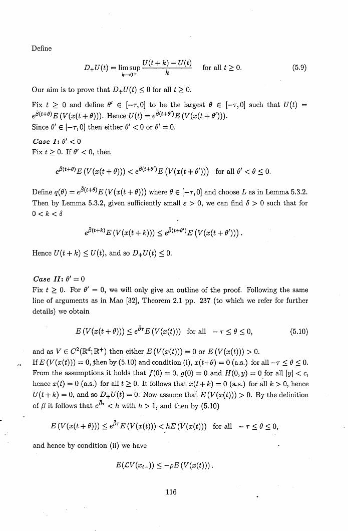
Define

D U(t) - l' U(t + k) - U(t) + - Imsup k

k-O+ for all t 2:: 0. (5.9)

Our aim is to prove that D+U(t) :5 0 for all t ;::: O.

Fix t ;::: 0 and define ()' E [-7,0] to be the largest () E [-7,0] such that U(t) =

eil(t+O) E (V(x(t + ()))). Hence U(t) = eil(t+o') E (V(x(t + ()'))). Since ()' E [-7,0] then either ()' < 0 or ()' = O.

Case I: ()' < ° Fix t 2:: 0. If ()' < 0, then

eil(t+O)E(V(x(t+()))) < eil(t+o')E(V(x(t+()'))) for all ()' < ():5 o.

Define q(O) = eil(t+()) E (V(x(t + ()))) where () E [-7,0] and choose L as in Lemma 5.3.2.

Then by Lemma 5.3.2, given sufficiently small c > 0, we can find 8 > ° such that for

0<k<8

Hence U(t + k) :5 U(t), and so D+U(t) :5 o.

Case II: ()' = ° Fix· t 2:: O. For ()' = 0, we will only give an outline of the proof. Following the same

line of arguments as in Mao [32], Theorem 2.1 pp. 237 (to which we refer for further

details) we obtain

E (V(x(t + ()))) :5 eilr E (V(x(t))) for all - 7 :5 () :5 0, (5.10)

and as V E C2 (JRdj JR+) then either E (V(x(t))) = 0 or E (V(x(t))) > 0.

If E (V(x(t))) = O,.then by (5.10) and condition (i), x(t+()) = ° (a.s.) for all-7 :::; () :::; 0.

From the assumptions it holds that 1(0) = 0, g(O) = ° and H(O, y) = 0Jor all Iyl < c,

hence x(t) = 0 (a.s.) for all t 2:: 0. It follows that x(t + k) = ° (a.s.) for all k > 0, hence

U(t + k) = 0, and so D+U(t) = O. Now assume that E (V(x(t))) > O. By the definition

of f3 it follows that eilr < h with h > 1, and then by (5.10)

E (V(x(t + ()))) :5 eilr E (V(x(t))) < hE (V(x(t))) for all - 7 :5 () :5 0,

and hence by condition (ii) we have

E(.cV(xt_)) :::; -pE (V(x(t))).

116

By applying Ito's formula to Z(t) = e,B(t+k)V(X(t + k)) for k > 0 we have the following

Hence by (5.7)

eiJ(t+k) E (V(x(t + k))) - eiJt E (V(x(t))) = l+k eiJa [.BE (V(x(s-))) + E(CV(xa-))] ds.

(5.11)

Now apply condition (ii) to see that

~E (V(x(t))) + E(CV(xt-)) ::; -(p - ~)E (V(x(t))) < 0 (5.12)

since p > ~. From this point we argue as in Mao [32] pp. 237 and the required result

follows. 0

The theorem below shows that under some additional assumptions, the pth moment

exponential stability, of the trivial solution of (5.1), implies the almost sure exponential

stability, generalizing Theorem 2.2 pp. 238 in Mao [32].

Theorem 5.3.4 Det p ~ 2. Assume that the hypotheses of Theorem 5.3.3 hold and

there exists constants Kl > 0 and K2 > 0 such that, for all ¢ E Li([-r, 0]; }Rd), the

following conditions are satisfied.

1?

(i) E (If(¢)IP) + E (tr [g(¢)T g(¢)]) ~ + E ({ IH(¢, Y)12 V(dY)) 2 ::; Kl sup E (I¢((})IP) . J1yl <c -r:::;O:::;O

(5.13)

(ii) E (r IH(¢, y)IP V(dY)) ~ K2 sup E (I¢((})IP) • (5.14) J1yl <c -r$O:::;O

117

Then

lim sup ~ log Ix(t)1 :::; _f!.. t-oo t p

a.s.

where f3 = min{p, log(h)/T}.

Proof: For t ~ T, by Jensen's inequality we can deduce that

E (11xHTln = E C~~~T Ix(t + h)IP) :5 4P-

1 (E (lx(t)IP) + E [[+T If(xs-)I dSr

+ E [sup I {t+h g(Xs_)dB(S)IP]

O~h~T it

+ E [sup {t+h { H (Xs-, y) N(ds, dy) P] ). O~h~T it J1yl<c

Using Holder's inequality, condition (5.13) and the results of Theorem 5.3.3, then

(5.15)

By the Burkholder-Davis-Gundy inequality (see Chapter 3, Theorem 3.5.3) and

following the same line of arguments that were used to deduce (5.15), we have

where Cp is a positive constant depending only on p.

The estimates in (5.15) and (5.16) are exactly the same estimates obtained in the

Bro~nian motion case, as in Mao [32] pp. 238-239.

Now for the compensated Poisson integral we will use Kunita's estimates (see Chapter

3, (3.43)). Applying Holder's inequality to the first term of the right-hand side of the

118

inequality below and then conditions (i) and (ii) we deduce that

E [sup 1t

+h 1 H (Xs-, y) N(ds, dy) P]

O$h$r t Iyl<c

:::; c3(P)E [ ([+T jYI<c IH (Xs-, Y) 12 11(dY)dS) ~]

+ c4(p)E [1t+

r 1 IH (~s-, y)IP V(dY)dS] t Iyl<c

:::; C3(P)T~-J E [[+7 (jYI<C IH (xs-, y)12 lI(dy) r dS]

+ c4(p)E [J. t+

r { IH (xs-, y)IP V(dY)dS]

t J1yl<c

::; C3(p)T~-1 (1t+

r Kl sup E(lx(s + O)IP)dS)

t -r$O$O

._ + C4(p) (11+7

K2_;~f:.:;o E(lx(s +B) IP) dS) , (5.17)

where C3(p) and C4(p) positive constants that depend on p.

Hence by (5.8) and (5.17) we obtain

E [sup 1t+hl H(xs_,y)N(ds,dy) P] ::; (C3(P)T~Kl +C4(p)TK2) qq21E(llxoIIP)e-/3(t-r). O$h$r t Iyl<c

Combining (5.15), (5.16) and (5.18) we find that

for all t 2:: T

where ~

L = 4P:~q2 E{lIx oIlP) [1 + ell7 (KJ (TP + CpT~ + C3(P)T~) + c4(p)K2T)].

From this point we follow Mao's exact arguments in [32] pp. 239 and the required result

follows. 0

119

(5.18)

5.4 Stochastic differential delay equations

In this section we consider stochastic differential delay equations (SDDE) driven by

Levy noise and examine their stability properties.

The first article on stochastic delay equations driven by Brownian motion was by Ito and

Nisio in [20]. In [15] Gushchin and Kuchler give necessary and sufficient conditions for

the existence of a stationary solution to an SDDE driven by a Levy process. Stationary and Feller properties of SDDEs driven by Levy processes can be found in Rei,8, Riedle

and Gaans [41], while Mohammed and Scheutzow in [38] discuss flow and stability

properties. For a detailed treatment of SDDEs we refer to these.

Now a general SDDE driven by Levy noise has the following form

dx(t) = F(x(t-),x(t- - Ill(t)), ... ,x(t- - Ilk(t)))dt

+G( x(t-), x( t- - III (t)), ... , x(t- - Ilk(t))) dB(t)

+ r K(x(t-),X(t--lll(t)),oo.,X(t--llk(t)),y)N(dt,dy) (5.19) J1yl<c "

for t 2:: 0, where for 1· ::; n ::; k, Iln : JR+ --+ [0,7] are continuous functions,

F: JRdx Md,k(JR) --+ JRd, G: JRdxMd,k(JR) --+ Md,m(JR) and H: JRdxMd,k(JR)xJRd --+ JRd

and the initial data Xo is a fixed V([-7, 0]; JRd)-valued random variable.

We assume that F(O, 0, ... ,0) = 0, G(O, 0, ... ,0) = 0 and K(O, 0, ... ,0,0) = 0 so that

for Xo = 0 we see that (5.19) admits a trivial solution.

Define for t 2:: 0, ¢ E V([-7, 0]; JRd)

f ( ¢) = F ( ¢t (0), ¢t ( - III ( t ) ), ... , ¢t ( - 11 k ( t) )), 9 ( ¢) = G ( ¢t (0), ¢t ( - III ( t ) ), ... , ¢t ( - Ilk ( t ) ) ) ,

Assume that F, G, H satisfy (F1) and (F2). Then (5.19) is of the same form as (5.1),

with coefficients given by j, g, H as defined previously. Hence, we can apply the results

that have been obtained in section 5.3 for SFDEs to examine the stability properties of

SDDEs.

120

..:>

In this case the functional .cV : V( [-r, 0]; JRd) -+ JR will have the following form

(.cV) (¢) = pi (¢(O), ¢( -ILl (t)), ... , ¢( -lLk(t))) (8i V)(¢(O))

+~ [G (q,(0) , q,( -/tl (t)), ... ,q,( -/tk(t))) G (q,(0), q,( -/tl(t)), ... ,q,( -/tk(t)) rf (8i8r V) (q,(0))

+ r [V(¢(O) +K(¢(O),¢(-ILI(t)), ... ,¢(-lLk(t)),y) - V(¢(O)) J1yl<c '

- Ki (¢(O), ¢( -ILl (t)), ... ,¢( -ILk (t)), y) (8i V)(¢(O))] lI(dy) (5.20)

where V E C 2(JRd; JR+), and ¢ E V([-r, 0]; JRd).

The following is a generalization of Mao's work [32], Theorem 3.1.

Theorem 5.4.1 Let V E C2(JRd; JR+), h > 1 and p, qb q2, p, Pb ... , Pn be positive

constants. If

and the functional .cv : V([-r, 0]; JRd) -+ JR as defined in (5.20) satisfies

k

(ii) (.cV) (¢) ~ -pV(¢(O)) + LPn V(¢( -lLn(t))) (5.21 ) n=l

where ¢ E V([-r, 0]; JRd), then the trivial solution of (5.19) is pth moment exponentially

stable if P > 2:~=1 Pn and moreover its pth moment Lyapunov exponent satisfies

lim sup ~ log(E (lx(t)I)P) < - (p - h t pn) t-oo t

n=l

a.s. (5.22)

where h E (1, pi 2:~=1 Pn) and is the unique solution of P - h 2:~=1 Pn = log(h)lr.

If p ~ 2 and the following conditions are satisfied for all (x, Zl, ... , Zk) E JRd x Md,k(JR)

with MI > 0, M2 > 0

, and

121

then the sample Lyapunov exponent

(

~k ) . 1 p - h L.J - Pn hmsup -log Ix(t)1 < _ n-l t-HX> t P

a.s.

If P - h L:~=1 Pn > 0 then the trivial solution of (5.19) is almost surely exponentially

stable.

Remark 5.4.2 The uniqueness of solution to p - h 2:~=1 Pn = log(h)/T is proved in

Appendix B.

Proof: For t 2:: 0, choose cPt E Lf([-T, 0]; JRd) which satisfies

E (V(cPt((}))) < hE (V(¢t(O))) for all - T ~ (} ~ 0 (5.25)

where h > 1. Then by (5.21) and (5.25), it holds that

k

E (c'V(cPt)) =::; -pE(V(cPt(O))) + L PnE(V(cPt( -jLn(t)))) n=l

(5.26)

Since p > 2:~=1 Pn and h E (1, p/ 2:~=1 Pn) then by (i), (5.25) and (5.26) the conditions

of Theorem 5.3.3 are satisfied, with /3 defined as /3 = min{p - h l:~=1 Pn, log(h)/T}.

It follows immediately that the trivial solution is pth moment exponentially stable and

the pth moment Lyapunov exponent satisfies

limsuP~log(E[lx(t)I]P) < - (P-h t pn) a.s. t-oo t

n=l

Now consider that.p 2:: 2. For all t 2:: 0 and cP E Lf([-T, 0]; JRd) then by (5.23), (5.24) and Jensen's inequality applied twice we can show that

E

E (If(<p)IP) + E (tr [g(<p)T g(<p)]) ~ + E ( ( I~(<p, Y) 12 l1(dY)) 2

J1yl<c

~ 3E ( M [I"'(OW + ~ 1"'( -JLn(t)) 12] ) ~ ~ 3M~ (1+ k)"? E (I"'(O)IP + t 1"'( -JLn(t))IP) ~ 3 (M(1+ k))! -:~f::;> (I"'(O)IP)'

122

where M = max{Mt, M2}. Also,

E (!rYI<c IH(cp, y)IP V (dy) ) < E ( M2 (I</>(OW + ~ I</>( -Jln(t))IP) )

~ (k + 1)M2 sup E (I¢(O)IP). -7":$0:$0

Hence, conditions (5.13) and (5.14) are satisfied and as the conditions of Theorem 5.3.3

hold, then by Theorem 5.3.4 the trivial solution of (5.19) is almost surely exponentially

stable, and so

.limsup ~ log Ix(t)1 :::; - (p - h ~~=1 pn) a.s. ~oo t P

o

5.5 Stabilization. of SFDEs by a Poisson process

Assume that we are given the following non-linear functional ODE system

on t~O (5.27)

with f : V([-r, 0]; JRd) ~ JRd and initial condition Xo E V([-r, 0]; JRd).

Consider that (5.27) is unstable, in the sense that as time increases indefinitely the

solutions of (5.27) escape to infinity.

Recent developments in the area of stochastic stabilization of SFDEs have been carried

out by Appleby [2]. Appleby considers an unstable functional ODE system and he

perturbs it with noise of the form ax(t)dB(t), where a =f 0 is a real number and B is a

one-dimensional standard Brownian motion. The system in homogenous form, for each

t ~ 0, is the following:

dx(t) = (fl(X(tj, x(t - rl(t)), ... , x(t - rn(t))) + it h(x(s))ds )dt + ax(t)dB(t) t-7"o(t)

where n E N. Appleby proves that if 11 and 12 satisfy global Lipschitz conditions

and global linear bounds and if the finite time delay r' = SUPt~O maxi=O,l, ... ,n ri(t) is sufficiently small, then we can choose a sufficiently large to stabilize the unstable

functional ODE system in an almost sure exponential way.

An improvement of Appleby's results has been made in [3] by Mao and Appleby. They

123

,.)

consider a more general stochastic perturbation of the form Ex(t)dB(t) with E E Md(JR) and for each t ~ 0, B(t) = (Bl(t), ... , Bm(t)) is an m-dimensional Brownian motion.

Namely, the stochastically perturbed system is

dx(t) = f(xt)dt + Ex(t)dB(t) (5.28)

with f(xt) = fl(X(t), x(t - rl(t)), ... , x(t - rn(t))) + ftt_ro(t) f2(X(s))ds, now satisfying

weaker conditions than the ones that Appleby imposed in [2]. To be precise, they

only require locally Lipschitz and one-sided linear bound conditions. In their work

[3] they have managed to stabilize (5.28) under certain conditions, and in particular,

they have shown that for E = aM, where a :f 0 and M E Md(JR) satisfying

minlxl=l (2{x, M x)2 - 1M x1 2) > 0, the solution of (5.28) tends to zero in an almost

sure exponential way when the noise intensity is large enough and the time delay is

sufficiently small.

Now, following Mao's and Appleby's ideas in [3] we will try and establish conditions

under which the unstable functional ODE sys~em (5.27) can be stabilized by Levy noise.

Remark 5.5.1 Note th~t from the Lipschitz condition on the drift coefficient and the

fact that f(O) = 0, it follows that f satisfies a one-sided linear bound i.e.

(<1>(0), f(<I») ::; 1<1>(0)1 If(<I» 1 ::; VLI(O)I·II<1>1I (5.29)

for every E V([-r, 0]; JRd), where L > 0 is as in (5.3), and (.,.) denotes the usual inner

product in JRd.

Many of the results of this chapter extend to SFDEs satisfying only local Lipschitz

conditions and a one-sided linear bound as in Mao and Appleby [3], where the Brownian

motion case is treated.

Assume the system (5.27) is perturbed by a one-dimensional compensated Poisson

process CN(t), t ~ 0) of intensity ..\ > O. Now, the new system forms a stochastic

functional differential equation i.e.

dx(t) = f(xt-)dt + Dx(t- )dN(t) for t ~ 0 (5.30)

with initial condition a fixed random variable Xo E V([-r, 0]; JRd). We take D E Md(JR)

to be a symmetric positive definite matrix with Pmin and Pmax its smallest and largest

eigenvalues respectively. Hence,

dx(t) = [J(Xt-) - "\Dx(t-)] dt + Dx(t- )dN(t). (5.31)

Existence and uniqueness of solutions to (5.30) follows from Theorem 5.2.2. Since

124

the drift coefficient in (5.30) satisfies (F1)-(F2) and the coefficient of the compensated

Poisson process is linear, then (5.30) admits a unique cadlag solution.

Remark 5.5.2 It was shown in Chapter 3 and Chapter 4, (Lemma 3.4.4 and Lemma

4.3.2) if the initial condition is non-zero, then the solution of an SDE driven by a Levy

process will be non-zero for all time. This property does not necessarily hold for SFDEs

(see Appleby [2]). Hence, we are not able to apply the, same method of proof that was

used in Chapter 4 for the stabilization of SDEs to the case of SFDEs.

N ow define for each t 2:: 0 and xo =I 0

{

lQtiill 8(t) = lX{t)f

80

for x(t) =I 0,

for x(t) = 0

{

2(xft),Dx(t» £ (t) --.L 0 c(t) = x(t)12 or x r,

cO for x(t) = 0

where 80 2:: 0 and cO 2:: 0 are such that 0 :5 80 :5 IIDII* and cO = 21IDII*. Note that for x(t) =I 0

IDx(t)12 = 8(t)2Ix(t)12 and 2{x(t), Dx(t)) = c(t)lx(t)12.

For x(t) =I 0, -c(t) :5 -2pmin and

log (c(t) + 8(t)2 + 1) = I (2{X(t), Dx(t)) + IDx(t)12 + 1) og Ix(t)12 Ix(t)12

(5.32)

(5.33)

(5.34)

<_ I (lx(t)12 + 21IDII*lx(t)12 + IIDII;.lx(t)12) = I (1 IIDII)2

og Ix(t)12 og + *

and for x(t) = 0

log (c(t) + <5(t)2 + 1) = log (CO + 802 + 1) :5 log(l + IIDII*)2 and

-c(t) = -co = -21IDII* :5 --2pmin.

Hence for all t 2:: 0 we have that

log (c(t) + 8(t)2 + 1) ::; log (1 + IIDII*)2 and - c(t) ::; -2pmin.

To establish stahilization of (5.30) we will follow the same line of arguments that were

used by Appleby and Mao in [3], Theorem 2.6, where they have proved the stabilization

of an unstable functional ODE system that is stochastically perturbed by Brownian

125

motion.

Theorem 5.5.3 The sample Lyapunov exponent of the solution of (5.30) satisfies

lim sup ~ log Ix(t)1 :::; - [.x (Pmin -log(1 + Pmax)) - VLexp (.xrpmax )] a.s. (5.35) t-oo t

In particular if .x (Pmin -log(1 + Pmax)) > VI exp (r .xpmax) then the trivial solution of

(5.30) is almost surely exponentially stable.

Proof: For Xo = 0 obviously (5.35) holds, since for each t ~ 0, x(t) = O. Consider now

that Xo =I O. Applying Ito's formula to Y(t) = Ix(t)12, we find, for each t ~ 0,

Ix{t)12 = Ixol2 + l [2(x{s- ),J{xs-)) - 2'x{x{s-), Dx{s-))] ds

+ l [lx(s-) + Dx(s- )12 - Ix(s- )12] dN(s)

= Ixol2 + l [2(x(s-), !(xs-)) - 2'x(x(s-), Dx(s-))] ds

+l [2x(s-)T Dx(s-) + IDx(s- )12) dN(s). (5.36)

Using (5.34) then (5.36) becomes

Y(t) = Y(O) + l [2(X(S-), !(xs-)) - ,xo(s-)Y(s-)] ds + l (o{s-) + o(s-)2)y(s_ )dN(s).

By the variation of constants formula for an SDE driven by a Poisson process (see

Chapter 2, Theorem 2.3.1), then, for each t ~ 0, we have

Y(t) = iJ>(t) [Y(O) + l2iJ>(S)-1(x(s-),!(xs-))dS] (5.37)

where by (2.20)

iJ>(t) = exp [-l 'xo(s- )ds + llOg (o(s-) + 0(s-)2 + 1 )dN{S)] . (5.38)

We extend the definition of to the whole of [-r,oo) by

{

exp [- J~ .xc(s- )ds + J~ log (c(s-) + 8(8-)2 + 1)dN(s)] for t ~ 0 (t) = .

1 for t E. [-r, 0] (5.39)

126

and define Z(t) = (t)-lY(t) for t ~ -T. Now by (5.37) and (5.29), for t ~ 0 we have

Z(t) < Y(O) + 2/£ l (s)-llx(s-)1·lIxs-lids

= Y(O) + 2/£ l (s)-LZ(s-)~ IIxs-11 ds.

From this point we will follow exactly the same arguments that were used by Appleby

and Mao in [3] pp. 1077 to obtain an estimate of the form

Z(t)! ~ IIxoll exp ( /£ l 9(S)dS) for t ~ 0 (5.40)

1 1 where for each t;::: 0, g(t) = (t)-2 SUPt_T~u~t(U)2. Since Z(t) = (t)-1Ix(t)12 then (5.40) becomes

Ix(t)1 ~ IIxoll(t)~ exp ( ..fL l 9(S)dS) for t ~ O. (5.41)

Hence combining (5.38) and (5.41), then

lim sup ~ log Ix(t)1 t-oo t

< lim sup ~ [- ~ ft £(s- )ds + ~ ft log (£(s-) + 8(s-)2 + l)dN(s) t-oo t 2 } 0 2 } 0

+ /£ l g(s)ds]. (5.42)

Now to obtain an estimate for the sample Lyapunov exponent of the solution of (5.30)

we must obtain an almost sure estimate for each of the terms on the right-hand side of

(5.42). From the way that £ is defined (see (5.33)) we see that

1lat

lim sup - -£(s-)ds ~ -2pmin. t-oo t 0

(5.43)

For the second term of the right-hand side of (5.42), by the strong law of large numbers

for a Poisson process (see Sato [42] pp. 246), it holds that

lim N(t) = ,\ t-oo t

a.s.

and hence,

li~:;,::p ~ [llOg (c(s-) +o(s-? + 1 )dN(s)] < li~:;,::p ~ [log(1+ IIDII.)2 N(t)]

= 2,\ log(l + Pmax). (5.44)

127

1 1 Recall that for each t ~ 0, g(t) = q?(t)-2" SUPt-r$u$t q?(U) 2" • Now for t ~ T

g(t) = exp G l >.c(8)d8 - ~ llOg (C(8-) H(8-)2 + 1 )dN(8»)

x sup exp (--21 [U Ac(s)ds +! [U log (c(s-) + 8(s-)2 + l)dN(S)) t-r$u$t Jo 2 Jo

= t_~~~~/xP G l >'c(S)d8) X t-~~~9 exp ( --~ llOg (C(8-) + 0(8-)2 + 1 )dN(8»)

< exp (>'IIDII.r) X t-~~~9 exp ( -lIOg(l + IIDII.)dN(8»)

< exp(AIIDII*T) = exp(TAPmax).

Hence,

11t 11t lim sup - g(s)ds ~ lim sup - exp (APmaxT) ds = exp (APmaxT). t-oo t 0 t-oo t 0

(5.45)

Applying (5.43), (5.44), and (5.45) into (5.42) then

lim sup ~ log Ix(t)1 ~. A(log(l + Pmax) - Pmin) + V£exp (APmaxT) t-oo t

a.s.

o

Remark 5.5.4 .To obtain almost sure exponential stability for the trivial solution of

(5.30) we can see from (5.35) that the time delay T has to be sufficiently small.

128

Appendix A

Existence and uniqueness of

SFDEs

In this section we will prove the existence and uniqueness of solutions of SFDEs driven

by Levy processes under the Lipschitz and growth conditions (Fl)-(F2). The proof is

based on Picard iteration and a combination of arguments used by Applebaum [1] pp.

305-309 in the proof of existence and uniqueness of SDEs driven by a Levy process, and

by Mao for SFDEs driven by Brownian motion in [33] pp. 150-152. Note that in the 1

proof below we are using II ·112 = (E(I'12)) 2 in L2(n,:F, P).

Theorem A.D.S Assume that the Lipschitz and growth conditions (Fl) and (F2) hold.

Then there exists a unique solution x = (x(t), t ~ -7) to (5.1) with initial data xo. The

process x is adapted and cddldg.

Proof of existence: Define a sequence of processes (xn, n E N U {O}) such that for each

t ~ 0, xO(t) = xo(O) and x~ = Xo and for each n E N U {O}, t ~ 0,

xn+l(t) = xo(O) +" rt f(x~_)ds + rt g(x~_)dB(s) + rt r H(x~_, y)N(ds, dy). Jo Jo Jo J1yl<c ,

(A.l)

Now each of the Ito integrals in (A.l) is a stochastic integral of a predictable process,

which by Applebaum [1] Theorem 4.2.3 and Theorem 4.2.12 is :Ft-adapted and has a cadlag modification. Using this property and a simple inductive argument we can show

that each xn, for n E N U {O}, is adapted and cadlag.

129

Now for each n E N U {O}, t ;::: 0, we have

xn+!(t) - xn(t) = l [f(x:_) - f(x::!)] ds + l [g(x:_) - g(x::!)] dB(s)

+ rt1. [H(x~_,y)-H(x~-=-1,y)]N(ds,dy). (A.2) Jo Iyl<c

We claim that for all n E N, t ;::: 0,

(A.3)

where C2(t) = tC1(t), C1(t) = 3t+24 and M = max{L,K (1 +E(lIxoIl2))} with L and K the Lipschitz and growth constants in (F1)-(F2) respectively.

We will show this by induction.

For n = 0, by (1.12), we deduce that

Ix 1(t) - xO(t)1 2 = [ft f(x~_)ds + rt g(x~_)dB(s) + rt 1. H(x~_, y)N(ds, dY)] 2 Jo Jo Jo Iyl<c

< 3{ [l f(xo)dsf + [l 9(Xo)dB(S)f

+ [ rt 1. H(xo, y)N(ds, dY)] 2 } (A.4) Jo Iyl<c

for each t ;::: 0 and -T ~ () ~ O. Firstly we take expectations. Then, for the drift

term we use the Cauchy-Schwarz inequality and for the other two terms apply Doobs's

martingale inequality (see Chapter 1, section 1.3) and then Ito's isometry property (see

Applebaum [1] Theorem 4.2.3). Finally an application of the linear growth condition

(F2) yields that

< 3t rt E (If(xo)12) ds + 12 rt E (lIg(xo)fl;) ds Jo . Jo

+12 rt r E (IH(xo,y)1 2) v(dy)ds Jo J1yl<c

< 3Kt l (1+ E (lixoIl2)) ds + 12K l (1+ E (lixoIl 2)) ds

+12K l (1+ E (lixoIl 2)) ds

= (3t + 24) Kt (1 + E (1IxoIl2)) = C1 (t)Kt (1 + E (lIxoI12))

130

where C1(t) = 3t + 24. Therefore

(A.5)

with C2(t) = tC1(t) and M = KE (1 + IIxoIl2).

Now we assume that (A.3) is true for arbitrary n E N and we will check that (A.3) holds

for n + 1. Hence,

Ixn+l(t) - xn(t) 12 = [l [f(x~_) - f(x~:l)] ds + l [g(x~_) - g(x~:l)l dB(s)

+ rt r [H(x~_, y) _ H(x~-=-I, y)] N(ds, dY)] 2 Jo J1yl<c

< 3{ [l [f(x~_) - f(x~.:l)l dsf + [l [g(x~_) - g(x~.:l)l dB(S)f

+ [rt r [H(x~_;y) _ H(x~-=-l,y)] N(dS,dY)]2

} • . ' 10 llyl<c

By the same arguments as was used in deducing (A.5),

[3E C~~~t {l' [J(x~-) - f(x~:l)l dU} 2)

+12E ( {l [g(x~_) - g(x~.:l)l dB(S)} 2)

+12E ( {l L<)H(X~_'Y) - H(x~.:I,Y)l N(ds,dy) f) ] < G1(t) [l E (I!(x~_) - f(x~.:l)n ds

+ l E(llg(x~_) - g(x~:l)II~)dS -

+ ft f E (l"H(X~_,y) - H(x~.:I,Y)n V(dY)dS] 10 J1yl<c

131

where Cl(t) = 3t + 24.

Now by the Lipschitz condition (F1) we have that

= Cl(t)£ rt E (.suP Ixn(u) - xn- 1(u)12

) ds, Jo O:5u:5s

(A.6)

and by the induction assumption we obtain

Hence (A.3) is true for all n E N.

Next we shall proof that '(xn(t), t ~ 0) is convergent in the £2 sense for each t ~ O. First

note that from (A.3) for each m, n E N and for each 0 :::; s :::; t we have that

Using a ratio test argument, we can see that the series on the right is a convergent

series. Consequently each (xn(s), n E N) is Cauchy and it follows immediately that it is

convergent to some x(s) E £2(O,F,P). Define x to be the process (x(t),t ~ 0). Hence

for each n E N U {O}, 0 :::; s :::; t,

In the next lines we will prove the almost sure convergence of (xn, n E N).

The Chebychev inequality and (A.3) yields that

Hence, by the Borel-Cantelli lemma

(2n)2 E (sup Ixn(s) - Xn- 1(s)12

) O:5s:5t

< (4C2(t)M)n n!

132

(A.8)

and it follows that

P (liminf sup Ixn(s) - xn-l(s)1 < 21 ) = 1. n-oo O~s~t n

Now given any 8 > 0 there exists no E N such that for any m, n > no we have that

with probability 1. As a result (xn, n E N) is almost surely uniformly Cauchy in finite

intervals [0, t] and hence almost surely uniformly convergent on finite intervals to the

process x = (x(t), t ~ 0). Since the uniform limit of a sequence of cadlag functions in a

finite interval is cadlag, then x is cadlag (see Applebaum [1] pp. 119). Also we can find

a subsequence (xnk , nk E N) for which the uniform convergence will still hold almost

surely, and hence x = (x(t), t ~ 0) is adapted (see Applebaum [1] pp. 71).

Now we need to show that x(t), for each t ~ 0, is a solution to (A.l). Denote by

x = (x(t), t ~ 0) the stochastic process given by

x(t) = xo(O) + rt f(xs-)ds + rt g(xs_)dB(s) + rt 1. H(xs-, y)N(ds, dy). Jo Jo Jo Iyl<c

Then, for each n E N U {O}, we obtain

x(t) - xn(t) = l [f(xs-) - f(x~-)l ds + l [g(xs-) - g(x~-)l dB(s)

+ rt 1. [H(xs-, y) - H(x~_, y)] N(ds, dy). Jo Iyl<c

Following the same arguments as used in deducing (A.6) i.e. the Cauchy-Schwarz

inequality, the It6)sometry property, the Lipschitz conditions and the result of (A.S),

then for all 0 :::; s :::; t :::; 00,

133

The right hand side of the inequality converges to 0 as n -+ 00, hence xes) =

L2 - limn_co xn(s). But from (A.8) each xes) = L2 - limn_co xn(s). Hence, by the

uniqueness of limits xes) = xes) almost surely for all 0 ~ s ~ t ~ 00.

Proof of uniqueness: Denote by x and x' two distinct solutions of (5.1). For each t ~ 0,

x'(t) - x(t) = l [f(x's-) - f(xs-)] ds + l [g(x's-) - g(xs-)] dB(s)

+ rt r [H(x' s-, y) - H(xs-, y)] N(ds, dy). Jo J1yl<c

Using the same arguments that were used to deduce (A.6), the Cauchy-Schwarz

inequality, the Ito isometry property and the Lipschitz conditions then we have that

E (sup Ix'(s) - x(s)12) ~ C1(t)L rot E (1Ix's- - xs_11 2

) ds O:5s:5t In

= C1(t)L rt E (sup Ix'(u) - x(u)1 2) ds.

Jo O:5u:5s

Applying the Gronwall's inequality then E (suPO:5s :5t Ix'(t) - x(t)12) = O. This yields

that x' (s) = x( s) for all 0 ~ s ~ t almost surely and hence for all -7 ~ S ~ t, since

both satisfy (5.1) with initial condition xo. Now using the continuity of probability we

deduce that

P (x'(t) = x(t) for all t ~ -r) = P ( n (x'(t) = x(t) for all - 7 ~ t ~ N)) = 1 NE N


In Chapter 5 we have considered "small" and "large" jumps under the same footing by

allowing c to take values in (0,00]. However, this is unnecessarily restrictive. Hence for

the sake of completeness we will show by interlacing that SFDEs that deal separately --

the "small" and "large" jumps of the Levy process have a unique solution. In this case

we can consider the whole class of Levy processes as driving noise.

Let z = (z(t), t ~ to) be the solution of

z(t) = zo(O) + rt f(zs- )ds + rt g(zs_)dB(s) + rt r H (zs-, y) N(ds, dy)

Jo Jo Jo J1yl<c

+ rt r K (zs-, y) N(ds, dy) on t ~ 0, (A.9) Jo JIYI~c

134

where Zo is the fixed initial condition, K : V([-T, 0]; ]Rd) x]Rd --+ ]Rd is Borel measurable

and the mappings /,9, H and the process B and the random measure N as defined in

Chapter 5.

Assumption A.O.6 We require that

x --+ K(x, y)

is a continuous mapping for all Iyl ~ c.

Theorem A.D.7 The solution of (A.9), Z = (z(t), t ;:::: 0) is a unique adapted cddldg

process.

Proof: Let (Tn, n E N) be the arrival times for the jumps of the compound Poisson

process (P(t), t ~ 0) where P(t) = ~YI~c yN(t, dy). Let x = (x(t), t ~ 0) be the solution

of (5.1) and z = (z(t), t ~ 0) be the solution of (A.9) with zo(O) = xo(O). Using the

interlacing technique (see Applebaum [1] pp. 311) we will construct a solution to the

SFDE (A.9) in the following way:

z(t) = x(t) for 0 ~ t < T1,

~(Tl) = X(TI-) + K (ZTl-' ~P(Tl)) for t = T1,

z(t) = z( Tl) + Xl (t) - Xl (Tl) for Tl < t < T2,

Z(T2) = Z(T2-) + K (ZT2-' ~P(T2)) for t = T2,

and so on recursively, where for each i E N, Xi is the solution of (5.1) with Xi(O) = Z(Ti)

and ZTi : n --+ V([-T, 0]; JRd) is defined as

for each wEn and () E [-T,O]. Now Z is a solution to (A.9) and is easily seen to be an

adapted and cadlag process. Note that assumption A.0.6 ensures the predictability of

the Poisson integrals. By the uniqueness of the s~lution of (5.1) (see Theorem A.0.5)

and the form of the interlacing structure, Z is unique. 0

135

Appendix B

A useful lemma

The following lemma applies for Theorem 5.4.1, Chapter 5.

Lemma B.D.S Let h > 1 and p, PI, ... ,Pk, T be positive constants. Then

k

P - h L Pn = log(h)/r (B.l) n=1

has a unique solution.

Proof: Let hI > 1 and h2 > 1 be two distinct solutions to (B.l). Hence,

k k

P - hI LPn = log(hl)/r and P - h2 L Pn = log(h2)/r. n=1 n=1

This implies that

(B.2)

Now if hI > h2 then for all hI, h2 > 1 we have that- r(hl - h2) l:~=1 Pn + log (~) > O.

If hI < h2 then for all hI, h2 > 1 we obtain that r(hl - h2) l:~=1 Pn + log (~) < O.

Hence, (B.2) is satisfied only if hI = h2. 0

136

Bibliography

[1] D. Applebaum. Levy processes and Stochastic Calculus. 1st edition. Cambridge

University Press, 2004, 2nd edition to appear in 2009.

[2] J. Appleby. Stabilization of functional differential equations by noise. System

Control Letters, in press.

[3] J. A. D. Appleby and X. Mao. Stochastic stabilization of functional differential

equations. Systems and Control Letters, 54:1069-1081, 2005.

[4] S. T. Ariaratnam and W. C. Xie. Almost-sure stochastic stability of coupled

non-linear oscillators. International Journal of Non-Linear Mechanics, 29:197-204,

1994.

[5] L. Arnold, H. Crauel, and V. Wihstutz. Stabilization of linear systems by noise.

SIAM Journal on Control and Optimization, 21:451-461, 1983.

[6] R. Bellman, J. Bentsman, and S. Meerkov. Stability for fast periodic systems.

IEEE Transactions on Automatic Control, AC-30:289-291, 1985.

[7] E. Boyce and R. Diprima. Elementary Differential Equations and Boundary Value

Problems. 2nd edition. Wiley, 1965.

[8] F. Brauer. Perturbations of non-linear systems of differential equ~tions. Journal

of Mathematical Analysis and Applications, 14:198-206, 1966.

[9] F. Brauer. Perturbations of non-linear systems of differential equations, II. Journal

of Mathematical Analysis and Applications, 17:418-434, 1967.

[10] J. C. Burkill. A First Course in Mathematical Analysis. Cambridge University

Press, 1962.

[11] P. Carr, H. Geman, D. B. Madan, and M. Yor. The fine structure of assets returns:

An empirical investigation. Journal of Business, 75:305-332, 2002.

[12] R. Cont and P. Tankov. Financial Modelling with Jump Processes. Chapman, 2004.

137

[13] M. Grigoriu. Lyapunov exponents for nonlinear systems with Poisson white noise.

Physics Letters A, 217:258-262, 1996.

[14] M. Grigoriu and G. Samorodnitsky. Stability of the trivial solution for

linear stochastic differential equations with Poisson white noise. Journal of

Physics:Mathematical and General, 37:8913-8928, 2004.

[15] A. A. Gushchin and U. Kuchler. On stationary solutions of delay differential

equations driven by Levy processes. Stochastic Processes and their Applications,

88:195-211, 2000.

[16] J. K. Hale and S. M. Lunel. Introduction to Functional Differential Equations.

Springer-Verlag, 1993.

[17] G. H. Hardy, J. E. Littlewood, and G. P6lya. Inequalities. 2nd edition, Cambridge

Mathematical Library, 1999.

[18] N. Ikeda and S. Watanabe. Stochastic Differential Equations and Diffusion

Processes. 2nd edition, North Holland-Kodansha, 1989.

[19] K. Ito. Introduction to Probability Theory. Cambridge University Press, 1984.

[20] K. Ito and M. Nisio. On stationary solutions of a stochastic differential equation.

Journal of Mathematic Kyoto University, 4:1-75, 1964.

[21] Y. Kazmerchuka, A. Swishchukb, and J. Wu. The pricing of options for securities

markets with delayed response. Mathematics and Computers in Simulation, 75:69-

79,2007.

[22] R. Z. Khasminski. Stochastic stability of Differential Equations. Alphen: Sojtjoff

and Noordhoff (1980), translation of the Russian edition, 1969.

,} [23] V. Kolmanovskii and V. R. Nosov. Stability of Functional Differential Equations.

Academic Press, 1986.

[24] F. Kozin. A survey of stability of stochastic systems. Automatica, 5:95-112, 1969.

[25] H. Kunita. Stochastic differential equations based on Levy processes and stochastic

flows of diffeomorphisms. Real and Stochastic Analysis, New Perspectives, M.M.Rao

(ed.):305-75, 1984.

[26] H. J. Kushner. Stochastic Stability and Control. Academic Press, 1967.

[27] A. E. Kyprianou. Introductory Lectures on Fluctuations of Levy processes with

Applications. Springer, 2006.

138

[28] C. W. Li, Z~ Dong, and R. Situ. Almost sure stability of linear stochastic differential

equations with jumps. Probability Theory and Related Fields, 123:121-155, 2002.

[29] R. Liptser. A strong law of large numbers for local martingales. Stochastics, 3:217-

228, 1980.

[30] D. B. Madan and E. Seneta. The variance gamma (v.g) model for share market

returns. The Journal of Business, 63:511-524, Oct., 1990).

[31] X. Mao. Stochastic stabilization and destabilization. Systems and Control Letters,

23:279-290, 1994.

[32] X. Mao. Razumikhin-type theorems on exponential stability of stochastic functional

differential equations. Stochastic Processes and Their Applications, 65:233-250,

1996.

[33] X. Mao. Stochastic Differential Equations and Applications. Horwood, 1997.

[34] X. Mao. Stability and stabilization of stochastic delay equations .. lET Control

Theory and Applications, 1:1551-1566, 2007.

[35] X. Mao and A. E. Rodkina. Exponential stability of stochastic differential equations

driven by discontinuous semimartingales. Stochastics and Stochastic Reports,

55:207-225, 1995.

[36] S. Meerkov. Condition of vibrational stabizability for a class of non-linear systems.

IEEE Transactions on Automatic Control, 27:485-487, 1982.

[37] S-E. A. Mohammed. Stochastic differential systems with memory. theory, examples

and applications. Stochastic Analysis and Related Topics VI. The Geilo Workshop,

1996.

[38] S-E. A. Mohammed and M. K. R. Scheutzow. Lyapunov exponents of linear .• stochastic functional differential equations. Part II. Examples a~d case studies.

The Annals of Probability, 27:1210-1240, 1997.

[39] A. D. Myshkis. Razumikhin's method in the qualitative theory of processes with

delay. Journal of Applied Mathematics and Stochastic Analysis, 8:233-247, 1995.

[40] P. Protter. Stochastic Integration and Differential Equations. Springer, 2000.

[41] M. Rei,B, M. Riedle, and O. van Gaans. Delay differential equations -driven by

Levy processes: stationarity and Feller properties. Stochastic Processes and their

Applications, 116:1409-1432, 2006.

[42] K. Sato. Levy process and Infinitely Divisible Distributions. Cambridge University

Press, 1999.

139

[43] J. La Selle and S. Lefschetz. Stability by Lyapunov's Direct Method. Academic

Press, 1961.

140

Documents

Stability properties of stochastic nOIse - CORE