Statistical characterization of the meteor trail distribution at the South Pole as seen by a VHF interferometric meteor radar

Statistical characterization of the meteor trail distribution at the

South Pole as seen by a VHF interferometric meteor radar

Elıas M. Lau,1 Susan K. Avery,1 James P. Avery,2 Diego Janches,3

Scott E. Palo,4 Robert Schafer,1 and Nikolai A. Makarov5

Received 29 January 2005; revised 14 January 2006; accepted 3 March 2006; published 19 July 2006.

[1] AVHF meteor radar system was installed at the geographical South Pole in 2001. Thepurpose of this system is to measure the horizontal wind field in the mesosphere–lower thermosphere (MLT) region and to understand the large-scale dynamics of theAntarctic polar region. The radar operated for a few months in 2001 and with minorinterruptions since that time. In this paper we will describe the meteor radar system, thedata detection and collection process, and the postprocessing software that was developedto extract information from the meteor echoes collected with the interferometer that ispart of the radar system. Finally, the main features of the meteor distribution will bepresented and discussed. Our results show that the meteor activity peaks during theAntarctic summer. Furthermore, it occurs mostly in a small region around the eclipticplane roughly �20� wide in terms of elevation angle spread.

Citation: Lau, E. M., S. K. Avery, J. P. Avery, D. Janches, S. E. Palo, R. Schafer, and N. A. Makarov (2006), Statistical

characterization of the meteor trail distribution at the South Pole as seen by a VHF interferometric meteor radar, Radio Sci., 41,

RS4007, doi:10.1029/2005RS003247.

1. Introduction

[2] Until recently there have been few studies of thepolar mesosphere– lower thermosphere (MLT, �80–120 km) using ground-based techniques. This has beendue in part to the harsh operating environment andgeographical remoteness of the region. In 1997 theNational Science Foundation (NSF) Coupling, Energet-ics and Dynamics of Atmospheric Regions (CEDAR)Phase III report identified the lack of measurements inthe polar regions as a deficiency that must be addressedif we are to further our understanding of the globallycoupled atmosphere-ionosphere system. The recommen-dations in this report, coupled with improved instrumentreliability and increased bandwidth to observational sites

have aided in deployment of more instruments to polarregions, mostly in the Arctic. This increase in observa-tions from the Arctic has begun to provide an improvedunderstanding of the dynamical processes important tothe Arctic region [Younger et al., 2002; Mitchell et al.,2002; Oznovich et al., 1997]. Continued long-termobservations are required if we are to understand thenormal circulation patterns of the polar mesosphere andthermosphere and to separate decadal-scale solar influ-ence from natural and anthropogenic secular changes.[3] While the network of MLT observing stations in

the Arctic has begun to mature, the Antarctic MLTobserving network is still in its infancy, with only fourMLT radars continuously operating in Antarctica. Thegoal of the meteor radar installed in 2001 (that is thefocus of this paper) is to continuously run at the SouthPole station and to utilize measurements of the MLTabove Antarctica to answer fundamental questions per-taining to Antarctic atmospheric dynamics.[4] Previous observations from the South Pole

[Hernandez et al., 1993; Portnyagin et al., 1997, 1998]have elucidated the presence of a large s = 1 westwardpropagating semidiurnal tide whose origin is unknown.This oscillation is not the typical solar forced migratingsemidiurnal tide (s = 2, westward) but rather a non-migrating semidiurnal tide, which is zonally coherentand present during the summer months but disappearsduring the winter months. When present in the summer

RADIO SCIENCE, VOL. 41, RS4007, doi:10.1029/2005RS003247, 2006

1Cooperative Institute for Research in Environmental Sciences,University of Colorado, Boulder, Colorado, USA.

2Department of Electrical and Computer Engineering, University ofColorado, Boulder, Colorado, USA.

3Colorado Research Associates Division, Northwest ResearchAssociates, Boulder, Colorado, USA.

4Department of Aerospace Engineering, University of Colorado,Boulder, Colorado, USA.

5Institute for Experimental Meteorology, Scientific ProductionAssociation TYPHOON, Obninsk, Russia.

Copyright 2006 by the American Geophysical Union.

0048-6604/06/2005RS003247

RS4007 1 of 19

this oscillation exhibits large temporal variations. Thesource of this nonmigrating semidiurnal tide, its seasonalstructure and temporal variations are unknown. Otherdynamical features such as eastward propagating plane-tary waves [Palo et al., 1998] and Lamb waves[Hernandez et al., 1992, 1996; Forbes et al., 1999] havealso been observed.[5] In September 2002 the first ever Southern Hemi-

sphere major stratospheric warming was observed[Baldwin et al., 2003]. This unprecedented event splitthe Antarctic ozone hole into two parts. The warmingwas 15 K larger than the only two previous minorstratospheric warmings observed in the previous 24years. Both temperature observations by Hernandez[2003] and wind observations by Dowdy et al.[2004] have indicated that the MLT dynamics weredifferent in 2002 when compared with previous years.There is also an indication that a reversal in the MLTzonal winds occurred approximately a week prior tothe warming [Dowdy et al., 2004]. This could indicatea possible dynamical connection between the strato-sphere and mesosphere prior to the warming. However,because of the short time series of Antarctic windmeasurements continued observations are required toestablish a baseline and understand the degree towhich the MLT was disturbed during 2002.[6] To improve our understanding of the Antarctic

dynamics a meteor radar system was installed at thegeographic South Pole in 2001 and has operated quasi-continuously since. In this paper we will describe theradar system, the detection and collection of the radarmeteor echoes. We will also discuss the processing usedto obtain the Doppler velocity and angle of arrival(AOA) estimates for each meteor echo. To obtain theseresults a precise calibration of the interferometer isneeded. We will compare two different calibration tech-niques used for those purposes. Finally, we present and

discuss the main statistical characteristics of the meteorpopulation observed by the radar at the South Pole.

2. Description of the Meteor Radar

[7] The South Pole VHF meteor radar system is aquasi all-sky system designed to measure the horizontalwind field in the MLT region. A detailed description ofthe radar system is given by Janches et al. [2004]. In thissection we will only summarize some of the moreimportant aspects of the radar.[8] The radar system is installed approximately 1 km

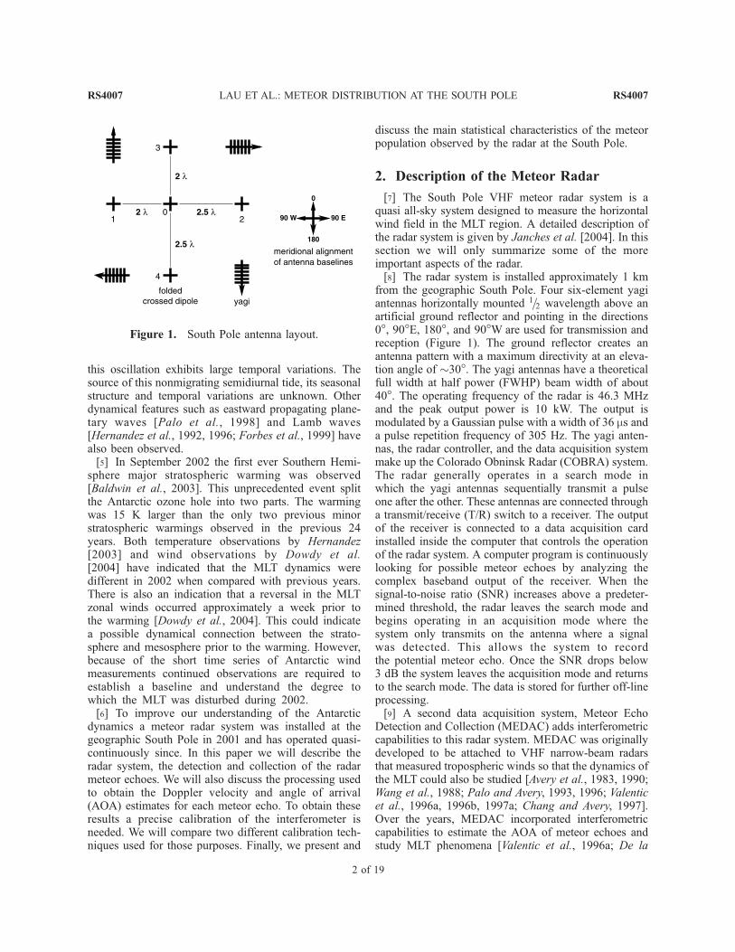
from the geographic South Pole. Four six-element yagiantennas horizontally mounted 1=2 wavelength above anartificial ground reflector and pointing in the directions0�, 90�E, 180�, and 90�W are used for transmission andreception (Figure 1). The ground reflector creates anantenna pattern with a maximum directivity at an eleva-tion angle of �30�. The yagi antennas have a theoreticalfull width at half power (FWHP) beam width of about40�. The operating frequency of the radar is 46.3 MHzand the peak output power is 10 kW. The output ismodulated by a Gaussian pulse with a width of 36 ms anda pulse repetition frequency of 305 Hz. The yagi anten-nas, the radar controller, and the data acquisition systemmake up the Colorado Obninsk Radar (COBRA) system.The radar generally operates in a search mode inwhich the yagi antennas sequentially transmit a pulseone after the other. These antennas are connected througha transmit/receive (T/R) switch to a receiver. The outputof the receiver is connected to a data acquisition cardinstalled inside the computer that controls the operationof the radar system. A computer program is continuouslylooking for possible meteor echoes by analyzing thecomplex baseband output of the receiver. When thesignal-to-noise ratio (SNR) increases above a predeter-mined threshold, the radar leaves the search mode andbegins operating in an acquisition mode where thesystem only transmits on the antenna where a signalwas detected. This allows the system to recordthe potential meteor echo. Once the SNR drops below3 dB the system leaves the acquisition mode and returnsto the search mode. The data is stored for further off-lineprocessing.[9] A second data acquisition system, Meteor Echo

Detection and Collection (MEDAC) adds interferometriccapabilities to this radar system. MEDAC was originallydeveloped to be attached to VHF narrow-beam radarsthat measured tropospheric winds so that the dynamics ofthe MLT could also be studied [Avery et al., 1983, 1990;Wang et al., 1988; Palo and Avery, 1993, 1996; Valenticet al., 1996a, 1996b, 1997a; Chang and Avery, 1997].Over the years, MEDAC incorporated interferometriccapabilities to estimate the AOA of meteor echoes andstudy MLT phenomena [Valentic et al., 1996a; De la

Figure 1. South Pole antenna layout.

RS4007 LAU ET AL.: METEOR DISTRIBUTION AT THE SOUTH POLE

2 of 19

RS4007

Pena et al., 2005]. For the South Pole radar, MEDAC isattached to an interferometer made up of 5 folded crosseddipoles in the cross configuration introduced by Jones etal. [1998] (Figure 1). MEDAC is used only for receptionand is synchronized with COBRA. MEDAC samplesranges between 80 and 461 km every 3 km and recordsfive complex traces for each detected echo: one for eachfolded crossed-dipole antenna. The traces are analyzedlater to obtain the AOA, height, and Doppler shiftcorresponding to each meteor echo.[10] While data is available from both systems, in this

paper we will focus on the data collected by the inter-ferometer attached to the MEDAC system.

3. Data Processing

[11] After detection a time series for each event isstored for off-line processing. Each meteor echo isanalyzed independently by the off-line postprocessingcode. The goal of this postprocessing code is to analyzeevery meteor echo that was collected in the field,determine its usability (if we have too few samples ofa meteor echo the estimation algorithms will not yielduseful results), and estimate atmospheric parametersassociated with it. For each detected meteor, we recordthe raw voltages coming out of the five receiversconnected to the five crossed-dipole antennas. Eachreceiver generates a complex baseband signal, referredto as the in-phase and quadrature signal.[12] Before the echo is subjected to any kind of

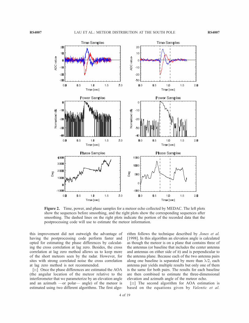
analysis we smooth the collected receiver outputs. Thetime series were smoothed using a 5-point runningaverage. In this paper we will often refer to the timeseries as the meteor trace or simply the trace. Power andphase sequences were then generated from the smoothedtime series. The power sequences were then smoothedusing a 5-point running average while the phase sequen-ces were smoothed using a 9-point running average. Thesmoothing reduces the noise level and increases theSNR. Hence we were able to increase the percentageof meteors that are detectable by the postprocessing codeand also reduce the estimation errors while keeping thesignals from being completely distorted. The windowsizes used for the smoothing were chosen heuristically.The effects of the smoothing are shown in Figure 2.[13] The next step in the echo postprocessing analysis

is the isolation of the echo itself since in the collecteddata we may have sections where only noise is present.To accomplish this we search for the peak in the powerprofile and we assume this is the start of the echo. Theend point of the echo is chosen to be the sample wherethe power drops below a 6 dB threshold above the noiselevel measured when the meteor was detected. This echoisolation process is depicted on the right plots of Figure 2where the signal between the dashed lines represents the

section of the collected data that is tagged as the meteorecho and is used for further postprocessing.[14] Once the echo is isolated its Doppler frequency fd,

because of the motion of the meteor trail, is estimatedusing four different techniques.[15] 1. Phase slope (PS): This method calculates the

instantaneous phase from each sample of the meteorecho time series and removes any 2p aliasing of thephase. The Doppler frequency is directly proportional tothe slope of the phase, that is, m = 2pfd. A linearregression is used to determine the phase slope fromthe phase measurements.[16] 2. Poly-pulse pair (PPP): The phase of the com-

plex autocorrelation function at lag ‘ and sampling timeTs is ff r = 2pfd‘Ts [Strauch et al., 1978]. We compute ff rfor lags ‘ = 0, 1, . . ., 5, and a least squares fit isperformed to this line to estimate the Doppler frequency.[17] 3. Maximum power spectral peak (MPSP): The

frequency at which the power spectrum peaks is assumedto be the frequency due to the Doppler shift of thereturned radar signal.[18] 4. Damped sinusoid (DS): An estimator that

iteratively estimates the Doppler frequency and decayrate of the meteor echo simultaneously [Tabei andMusicus, 1996].[19] The line-of-sight or radial velocity vr can then be

calculated from the estimated Doppler frequency throughthe equation vr = lfd/2, where l is the radar wavelengthand vr > 0 when the meteor trail moves toward the radar.[20] Because of system noise and different antenna

sensitivities the meteor does not usually start and end onthe same sample for all traces collected by the fiveantennas of the interferometer. For the postprocessinganalysis to continue it is required that the echoes em-bedded in all pairs of traces (in this paper we will refer toa pair as a couple consisting of the center antenna andany of the other ones) overlap for at least five samples. Ifthis condition is met, then the phase differences for eachpair of antennas are calculated by cross correlation at lagzero. The phase differences can also be calculated asthe mean of the sequence created by subtracting theunwrapped phase values for the corresponding antennapairs. In tests (not shown here) we have conducted usingsimulated meteor echoes the cross correlation at lag zeroproved to be the more accurate of the two approaches inthe presence of noise. A third way of calculating thephase differences is calculating the cross correlation for afew different lags, perform a linear regression fit, andthen calculate the fitted value at lag zero. For thisapproach, our simulations only show a marginal increasein accuracy while being more computationally taxing.Tests were also performed on actual meteor data and thedifference in the estimates of phase differences calculated;our results show that 93% of the differences are within2� and 97% are within 3�. Therefore we decided that


3 of 19

RS4007

this improvement did not outweigh the advantage ofhaving the postprocessing code perform faster andopted for estimating the phase differences by calculat-ing the cross correlation at lag zero. Besides, the crosscorrelation at lag zero method allows us to keep moreof the short meteors seen by the radar. However, forsites with strong correlated noise the cross correlationat lag zero method is not recommended.[21] Once the phase differences are estimated the AOA

(the angular location of the meteor relative to theinterferometer that we parameterize by an elevation angleand an azimuth —or polar— angle) of the meteor isestimated using two different algorithms. The first algo-

rithm follows the technique described by Jones et al.[1998]. In this algorithm an elevation angle is calculatedas though the meteor is on a plane that contains three ofthe antennas (or baseline that includes the center antennaand antennas on either side of it) and is perpendicular tothe antenna plane. Because each of the two antenna pairsalong one baseline is separated by more than l/2, eachantenna pair yields multiple results but only one of themis the same for both pairs. The results for each baselineare then combined to estimate the three-dimensionalelevation and azimuth angle of the meteor echo.[22] The second algorithm for AOA estimation is

based on the equations given by Valentic et al.

Figure 2. Time, power, and phase samples for a meteor echo collected by MEDAC. The left plotsshow the sequences before smoothing, and the right plots show the corresponding sequences aftersmoothing. The dashed lines on the right plots indicate the portion of the recorded data that thepostprocessing code will use to estimate the meteor information.


4 of 19

RS4007

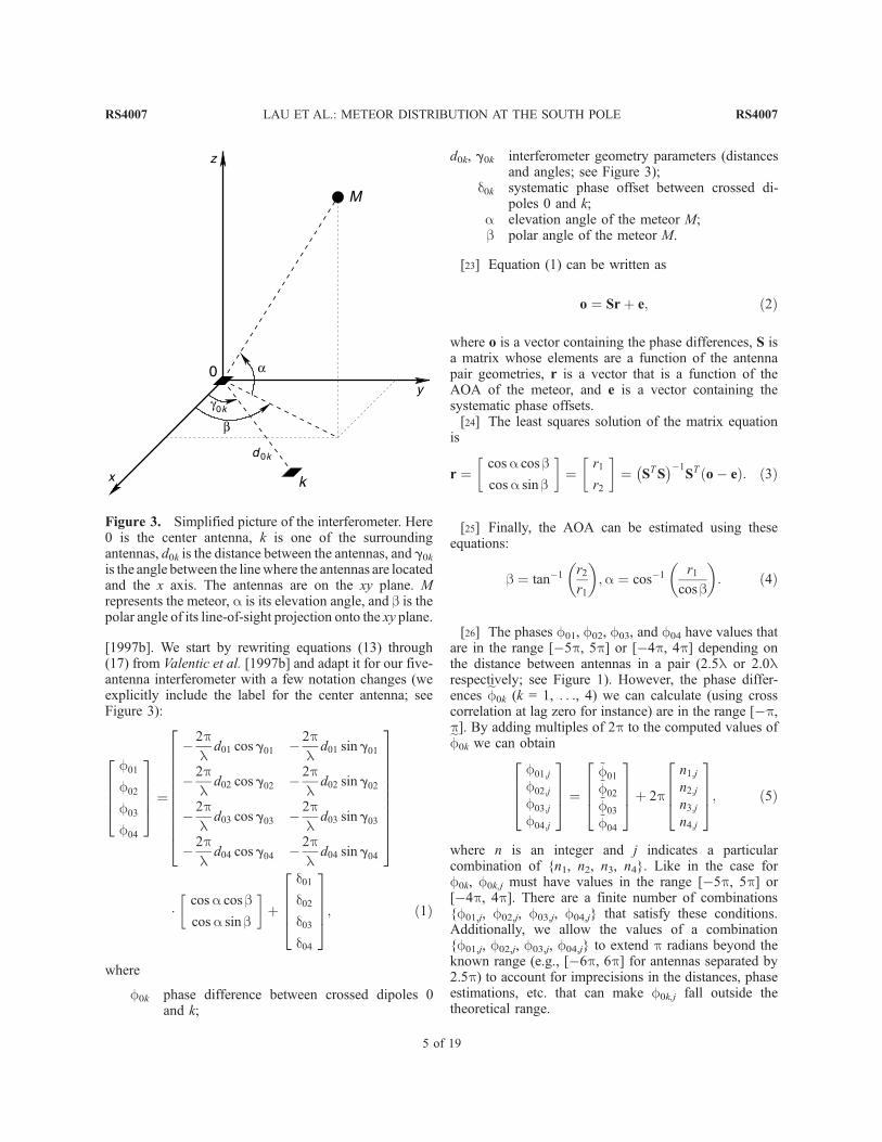
[1997b]. We start by rewriting equations (13) through(17) from Valentic et al. [1997b] and adapt it for our five-antenna interferometer with a few notation changes (weexplicitly include the label for the center antenna; seeFigure 3):

f01

f02

f03

f04

26664

37775 ¼

� 2pl

d01 cos g01 � 2pl

d01 sin g01

� 2pl

d02 cos g02 � 2pl

d02 sin g02

� 2pl

d03 cos g03 � 2pl

d03 sin g03

� 2pl

d04 cos g04 � 2pl

d04 sin g04

266666666664

377777777775

�cosa cos b

cosa sin b

� �þ

d01d02d03d04

26664

37775; ð1Þ

where

f0k phase difference between crossed dipoles 0and k;

d0k, g0k interferometer geometry parameters (distancesand angles; see Figure 3);

d0k systematic phase offset between crossed di-poles 0 and k;

a elevation angle of the meteor M;b polar angle of the meteor M.

[23] Equation (1) can be written as

o ¼ Srþ e; ð2Þ

where o is a vector containing the phase differences, S isa matrix whose elements are a function of the antennapair geometries, r is a vector that is a function of theAOA of the meteor, and e is a vector containing thesystematic phase offsets.[24] The least squares solution of the matrix equation

is

r ¼cosa cos bcosa sin b

� �¼

r1

r2

� �¼ STS

�1ST o� eð Þ: ð3Þ

[25] Finally, the AOA can be estimated using theseequations:

b ¼ tan�1 r2

r1

� �;a ¼ cos�1 r1

cos b

� �: ð4Þ

[26] The phases f01, f02, f03, and f04 have values thatare in the range [�5p, 5p] or [�4p, 4p] depending onthe distance between antennas in a pair (2.5l or 2.0lrespectively; see Figure 1). However, the phase differ-ences ef0k (k = 1, . . ., 4) we can calculate (using crosscorrelation at lag zero for instance) are in the range [�p,p]. By adding multiples of 2p to the computed values ofef0k we can obtain

f01;j

f02;j

f03;j

f04;j

2664

3775 ¼

~f01~f02~f03~f04

2664

3775þ 2p

n1;jn2;jn3;jn4;j

2664

3775; ð5Þ

where n is an integer and j indicates a particularcombination of {n1, n2, n3, n4}. Like in the case forf0k, f0k,j must have values in the range [�5p, 5p] or[�4p, 4p]. There are a finite number of combinations{f01,j, f02,j, f03,j, f04,j} that satisfy these conditions.Additionally, we allow the values of a combination{f01,j, f02,j, f03,j, f04,j} to extend p radians beyond theknown range (e.g., [�6p, 6p] for antennas separated by2.5p) to account for imprecisions in the distances, phaseestimations, etc. that can make f0k,j fall outside thetheoretical range.

Figure 3. Simplified picture of the interferometer. Here0 is the center antenna, k is one of the surroundingantennas, d0k is the distance between the antennas, and g0kis the angle between the linewhere the antennas are locatedand the x axis. The antennas are on the xy plane. Mrepresents the meteor, a is its elevation angle, and b is thepolar angle of its line-of-sight projection onto the xy plane.


5 of 19

RS4007

[27] We can now estimate the AOA (aj and bj) usingequation (4) if we substitute f0k,j for f0k in equation (1).We can replace the calculated values of aj and bj inequation (1) and generate f0k,j.[28] We define the error function in the estimated

phase values as

Ej ¼X4k¼1

f0k;j � f0k;j

� �2

: ð6Þ

[29] In theory, for a certain j = J we will have EJ = 0when f0k = f0k,J for k = 1, . . ., 4. This is equivalent tosaying that when our guess for the AOA is the same asthe actual AOA the error in the unwrapped phases goesto zero. Any other guess that does not coincide with theactual AOAwill lead to a positive error, that is, Ej 6¼J > 0.So, theoretically, we would aim for a combination ofunwrapped phases that gives Ej=J = 0. However, inpractice, for that value of j = J, Ej=J > 0 because of theuncertainties in the values of d0k, g0k, d0k, and ef0k.Therefore we choose the value of j that minimizes theerror Ej.[30] Applying trigonometry we utilize the estimated

elevation angle and the measured echo range to calculatethe vertical height of the meteor trail (see Appendix A).Since the ranges and zenith angles are large we cannotapproximate the true height as the distance above a flatEarth. By taking into account the curvature of the Earthwe define and calculate height as the distance in theradial direction above a spherical Earth of radius6378.1 km.

4. Testing of the Postprocessing Code

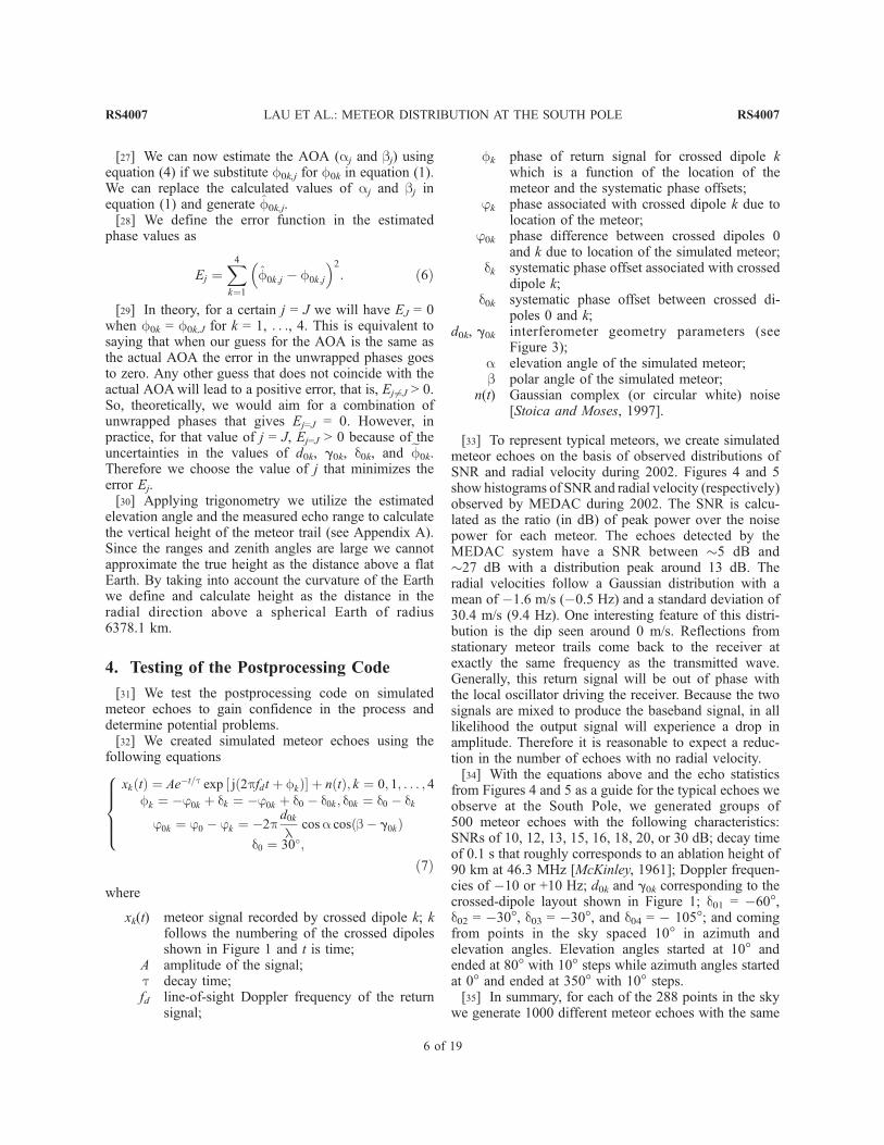
[31] We test the postprocessing code on simulatedmeteor echoes to gain confidence in the process anddetermine potential problems.[32] We created simulated meteor echoes using the

following equations

xk tð Þ ¼ Ae�t=t exp jð2pfdt þ fk½ Þ� þ n tð Þ; k ¼ 0; 1; . . . ; 4fk ¼ �j0k þ dk ¼ �j0k þ d0 � d0k ; d0k ¼ d0 � dk

j0k ¼ j0 � jk ¼ �2pd0k

lcosa cos b� g0kð Þ

d0 ¼ 30�;

8>>><>>>:

ð7Þ

where

xk(t) meteor signal recorded by crossed dipole k; kfollows the numbering of the crossed dipolesshown in Figure 1 and t is time;

A amplitude of the signal;t decay time;fd line-of-sight Doppler frequency of the return

signal;

fk phase of return signal for crossed dipole kwhich is a function of the location of themeteor and the systematic phase offsets;

jk phase associated with crossed dipole k due tolocation of the meteor;

j0k phase difference between crossed dipoles 0and k due to location of the simulated meteor;

dk systematic phase offset associated with crosseddipole k;

d0k systematic phase offset between crossed di-poles 0 and k;

d0k, g0k interferometer geometry parameters (seeFigure 3);

a elevation angle of the simulated meteor;b polar angle of the simulated meteor;

n(t) Gaussian complex (or circular white) noise[Stoica and Moses, 1997].

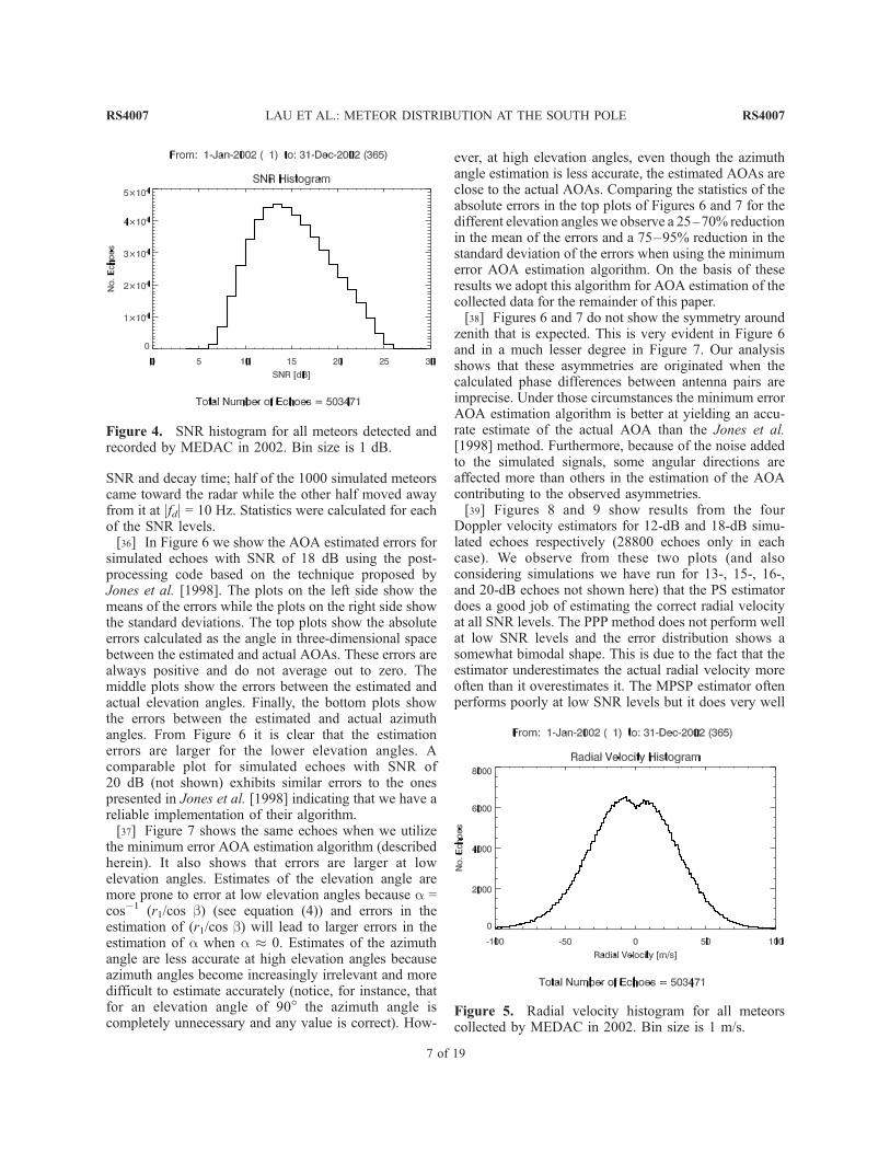
[33] To represent typical meteors, we create simulatedmeteor echoes on the basis of observed distributions ofSNR and radial velocity during 2002. Figures 4 and 5show histograms of SNR and radial velocity (respectively)observed by MEDAC during 2002. The SNR is calcu-lated as the ratio (in dB) of peak power over the noisepower for each meteor. The echoes detected by theMEDAC system have a SNR between �5 dB and�27 dB with a distribution peak around 13 dB. Theradial velocities follow a Gaussian distribution with amean of �1.6 m/s (�0.5 Hz) and a standard deviation of30.4 m/s (9.4 Hz). One interesting feature of this distri-bution is the dip seen around 0 m/s. Reflections fromstationary meteor trails come back to the receiver atexactly the same frequency as the transmitted wave.Generally, this return signal will be out of phase withthe local oscillator driving the receiver. Because the twosignals are mixed to produce the baseband signal, in alllikelihood the output signal will experience a drop inamplitude. Therefore it is reasonable to expect a reduc-tion in the number of echoes with no radial velocity.[34] With the equations above and the echo statistics

from Figures 4 and 5 as a guide for the typical echoes weobserve at the South Pole, we generated groups of500 meteor echoes with the following characteristics:SNRs of 10, 12, 13, 15, 16, 18, 20, or 30 dB; decay timeof 0.1 s that roughly corresponds to an ablation height of90 km at 46.3 MHz [McKinley, 1961]; Doppler frequen-cies of �10 or +10 Hz; d0k and g0k corresponding to thecrossed-dipole layout shown in Figure 1; d01 = �60�,d02 = �30�, d03 = �30�, and d04 = � 105�; and comingfrom points in the sky spaced 10� in azimuth andelevation angles. Elevation angles started at 10� andended at 80� with 10� steps while azimuth angles startedat 0� and ended at 350� with 10� steps.[35] In summary, for each of the 288 points in the sky

we generate 1000 different meteor echoes with the same


6 of 19

RS4007

SNR and decay time; half of the 1000 simulated meteorscame toward the radar while the other half moved awayfrom it at jfdj = 10 Hz. Statistics were calculated for eachof the SNR levels.[36] In Figure 6 we show the AOA estimated errors for

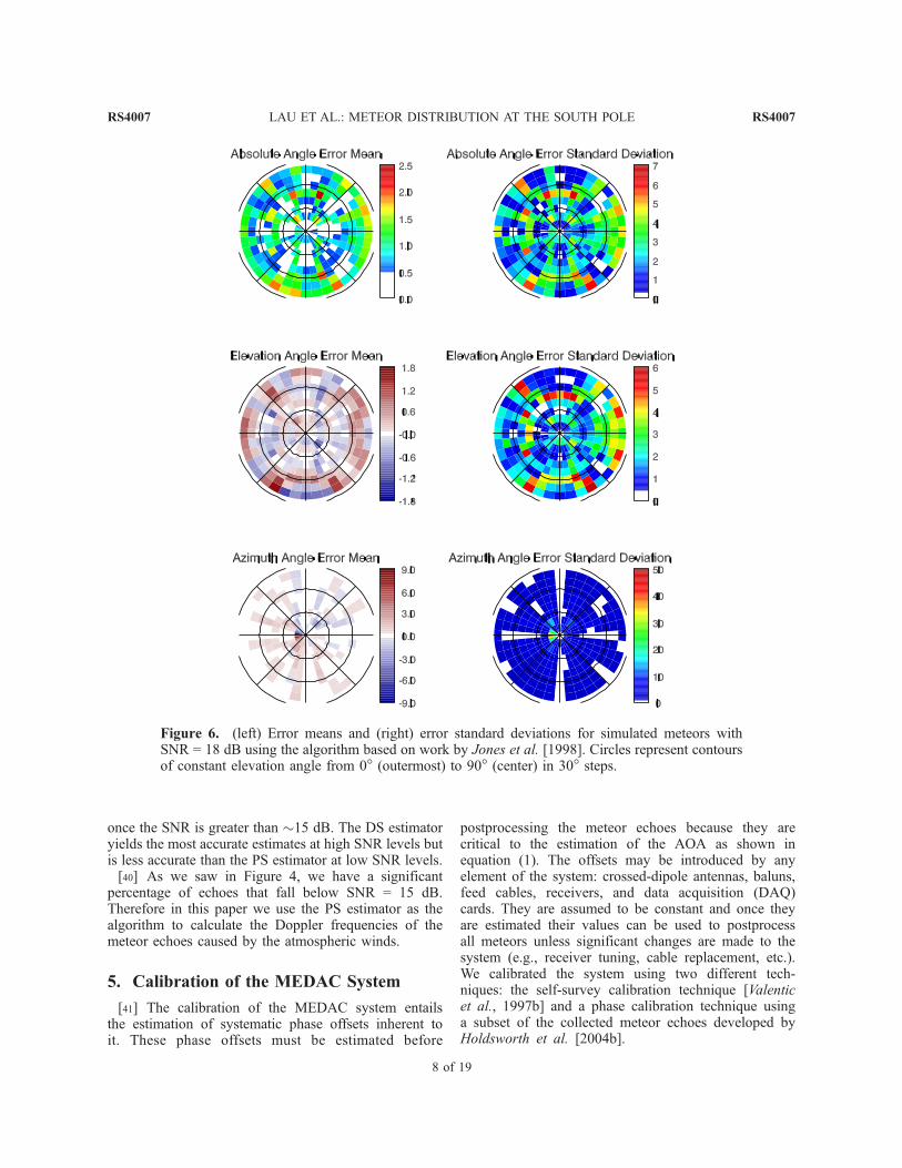
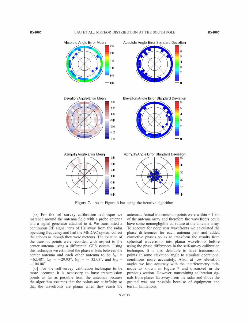
simulated echoes with SNR of 18 dB using the post-processing code based on the technique proposed byJones et al. [1998]. The plots on the left side show themeans of the errors while the plots on the right side showthe standard deviations. The top plots show the absoluteerrors calculated as the angle in three-dimensional spacebetween the estimated and actual AOAs. These errors arealways positive and do not average out to zero. Themiddle plots show the errors between the estimated andactual elevation angles. Finally, the bottom plots showthe errors between the estimated and actual azimuthangles. From Figure 6 it is clear that the estimationerrors are larger for the lower elevation angles. Acomparable plot for simulated echoes with SNR of20 dB (not shown) exhibits similar errors to the onespresented in Jones et al. [1998] indicating that we have areliable implementation of their algorithm.[37] Figure 7 shows the same echoes when we utilize

the minimum error AOA estimation algorithm (describedherein). It also shows that errors are larger at lowelevation angles. Estimates of the elevation angle aremore prone to error at low elevation angles because a =cos�1 (r1/cos b) (see equation (4)) and errors in theestimation of (r1/cos b) will lead to larger errors in theestimation of a when a � 0. Estimates of the azimuthangle are less accurate at high elevation angles becauseazimuth angles become increasingly irrelevant and moredifficult to estimate accurately (notice, for instance, thatfor an elevation angle of 90� the azimuth angle iscompletely unnecessary and any value is correct). How-

ever, at high elevation angles, even though the azimuthangle estimation is less accurate, the estimated AOAs areclose to the actual AOAs. Comparing the statistics of theabsolute errors in the top plots of Figures 6 and 7 for thedifferent elevation angles we observe a 25–70% reductionin the mean of the errors and a 75–95% reduction in thestandard deviation of the errors when using the minimumerror AOA estimation algorithm. On the basis of theseresults we adopt this algorithm for AOA estimation of thecollected data for the remainder of this paper.[38] Figures 6 and 7 do not show the symmetry around

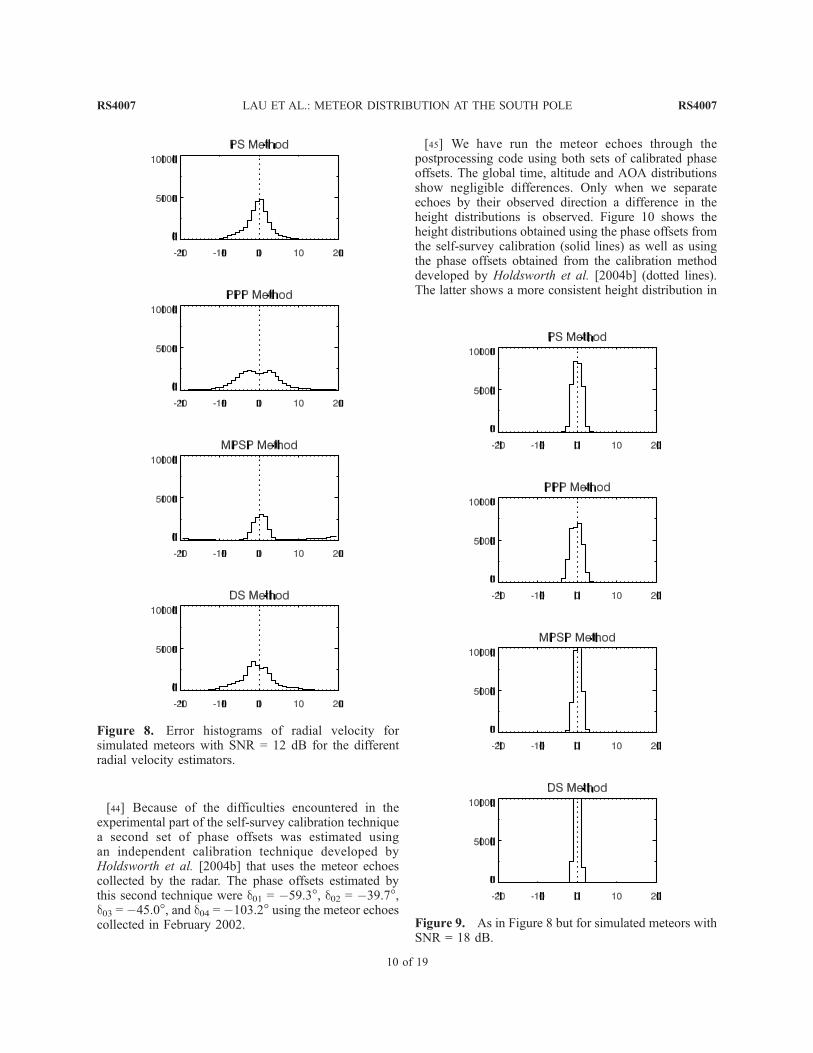
zenith that is expected. This is very evident in Figure 6and in a much lesser degree in Figure 7. Our analysisshows that these asymmetries are originated when thecalculated phase differences between antenna pairs areimprecise. Under those circumstances the minimum errorAOA estimation algorithm is better at yielding an accu-rate estimate of the actual AOA than the Jones et al.[1998] method. Furthermore, because of the noise addedto the simulated signals, some angular directions areaffected more than others in the estimation of the AOAcontributing to the observed asymmetries.[39] Figures 8 and 9 show results from the four

Doppler velocity estimators for 12-dB and 18-dB simu-lated echoes respectively (28800 echoes only in eachcase). We observe from these two plots (and alsoconsidering simulations we have run for 13-, 15-, 16-,and 20-dB echoes not shown here) that the PS estimatordoes a good job of estimating the correct radial velocityat all SNR levels. The PPP method does not perform wellat low SNR levels and the error distribution shows asomewhat bimodal shape. This is due to the fact that theestimator underestimates the actual radial velocity moreoften than it overestimates it. The MPSP estimator oftenperforms poorly at low SNR levels but it does very well

Figure 4. SNR histogram for all meteors detected andrecorded by MEDAC in 2002. Bin size is 1 dB.

Figure 5. Radial velocity histogram for all meteorscollected by MEDAC in 2002. Bin size is 1 m/s.


7 of 19

RS4007

once the SNR is greater than �15 dB. The DS estimatoryields the most accurate estimates at high SNR levels butis less accurate than the PS estimator at low SNR levels.[40] As we saw in Figure 4, we have a significant

percentage of echoes that fall below SNR = 15 dB.Therefore in this paper we use the PS estimator as thealgorithm to calculate the Doppler frequencies of themeteor echoes caused by the atmospheric winds.

5. Calibration of the MEDAC System

[41] The calibration of the MEDAC system entailsthe estimation of systematic phase offsets inherent toit. These phase offsets must be estimated before

postprocessing the meteor echoes because they arecritical to the estimation of the AOA as shown inequation (1). The offsets may be introduced by anyelement of the system: crossed-dipole antennas, baluns,feed cables, receivers, and data acquisition (DAQ)cards. They are assumed to be constant and once theyare estimated their values can be used to postprocessall meteors unless significant changes are made to thesystem (e.g., receiver tuning, cable replacement, etc.).We calibrated the system using two different tech-niques: the self-survey calibration technique [Valenticet al., 1997b] and a phase calibration technique usinga subset of the collected meteor echoes developed byHoldsworth et al. [2004b].

Figure 6. (left) Error means and (right) error standard deviations for simulated meteors withSNR = 18 dB using the algorithm based on work by Jones et al. [1998]. Circles represent contoursof constant elevation angle from 0� (outermost) to 90� (center) in 30� steps.


8 of 19

RS4007

[42] For the self-survey calibration technique wemarched around the antenna field with a probe antennaand a signal generator attached to it. We transmitted acontinuous RF signal tens of Hz away from the radaroperating frequency and had the MEDAC system collectthe echoes as though they were meteors. The location ofthe transmit points were recorded with respect to thecenter antenna using a differential GPS system. Usingthis technique we estimated the phase offsets between thecenter antenna and each other antenna to be d01 =�62.48�, d02 = �29.93�, d03 = � 32.03�, and d04 =�104.08�.[43] For the self-survey calibration technique to be

more accurate it is necessary to have transmissionpoints as far as possible from the antennas becausethe algorithm assumes that the points are at infinity sothat the wavefronts are planar when they reach the

antennas. Actual transmission points were within �1 kmof the antenna array and therefore the wavefronts couldhave some nonnegligible curvature at the antenna array.To account for nonplanar wavefronts we calculated thephase differences for each antenna pair and addedcorrective phases so as to transform the results fromspherical wavefronts into planar wavefronts beforeusing the phase differences in the self-survey calibrationtechnique. It is also desirable to have transmissionpoints at some elevation angle to simulate operationalconditions more accurately. Also, at low elevationangles we lose accuracy with the interferometry tech-nique as shown in Figure 7 and discussed in theprevious section. However, transmitting calibration sig-nals from places far away from the radar and above theground was not possible because of equipment andterrain limitations.

Figure 7. As in Figure 6 but using the iterative algorithm.


9 of 19

RS4007

[44] Because of the difficulties encountered in theexperimental part of the self-survey calibration techniquea second set of phase offsets was estimated usingan independent calibration technique developed byHoldsworth et al. [2004b] that uses the meteor echoescollected by the radar. The phase offsets estimated bythis second technique were d01 = �59.3�, d02 = �39.7�,d03 = �45.0�, and d04 = �103.2� using the meteor echoescollected in February 2002.

[45] We have run the meteor echoes through thepostprocessing code using both sets of calibrated phaseoffsets. The global time, altitude and AOA distributionsshow negligible differences. Only when we separateechoes by their observed direction a difference in theheight distributions is observed. Figure 10 shows theheight distributions obtained using the phase offsets fromthe self-survey calibration (solid lines) as well as usingthe phase offsets obtained from the calibration methoddeveloped by Holdsworth et al. [2004b] (dotted lines).The latter shows a more consistent height distribution in

Figure 8. Error histograms of radial velocity forsimulated meteors with SNR = 12 dB for the differentradial velocity estimators.

Figure 9. As in Figure 8 but for simulated meteors withSNR = 18 dB.


10 of 19

RS4007

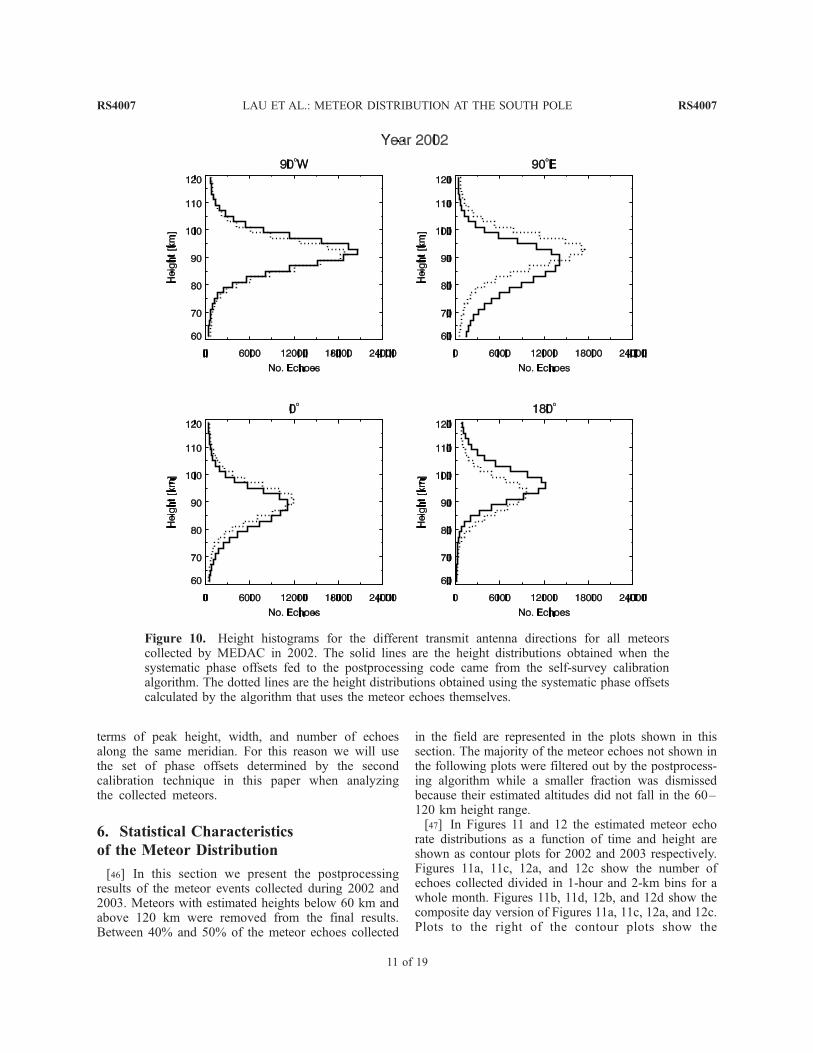
terms of peak height, width, and number of echoesalong the same meridian. For this reason we will usethe set of phase offsets determined by the secondcalibration technique in this paper when analyzingthe collected meteors.

6. Statistical Characteristics

of the Meteor Distribution

[46] In this section we present the postprocessingresults of the meteor events collected during 2002 and2003. Meteors with estimated heights below 60 km andabove 120 km were removed from the final results.Between 40% and 50% of the meteor echoes collected

in the field are represented in the plots shown in thissection. The majority of the meteor echoes not shown inthe following plots were filtered out by the postprocess-ing algorithm while a smaller fraction was dismissedbecause their estimated altitudes did not fall in the 60–120 km height range.[47] In Figures 11 and 12 the estimated meteor echo

rate distributions as a function of time and height areshown as contour plots for 2002 and 2003 respectively.Figures 11a, 11c, 12a, and 12c show the number ofechoes collected divided in 1-hour and 2-km bins for awhole month. Figures 11b, 11d, 12b, and 12d show thecomposite day version of Figures 11a, 11c, 12a, and 12c.Plots to the right of the contour plots show the

Figure 10. Height histograms for the different transmit antenna directions for all meteorscollected by MEDAC in 2002. The solid lines are the height distributions obtained when thesystematic phase offsets fed to the postprocessing code came from the self-survey calibrationalgorithm. The dotted lines are the height distributions obtained using the systematic phase offsetscalculated by the algorithm that uses the meteor echoes themselves.


11 of 19

RS4007

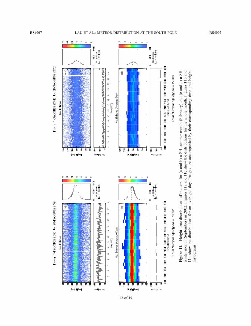
Figure

11.

Height-timedistributionsofmeteors

for(a

andb)aSH

summer

month

(February)and(c

andd)aSH

wintermonth

(September)in

2002.Figures11aand11cshowthedistributionsforthewholemonth.Figures11band

11dshow

thedistributionsforan

averaged

day.Im

ages

areaccompaniedbytheircorrespondingtimeandheight

histograms.


12 of 19

RS4007

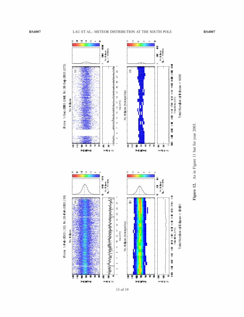
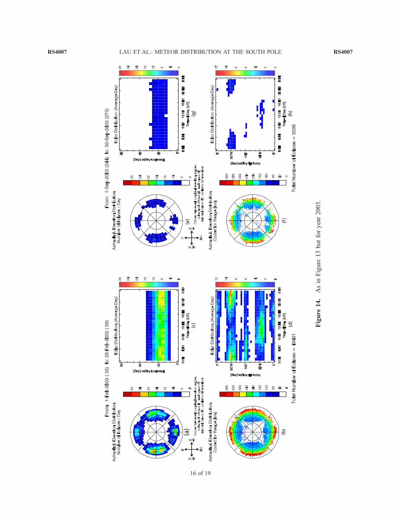
Figure

12.

Asin

Figure

11butforyear2003.


13 of 19

RS4007

corresponding height distributions independent of time,while plots underneath the contour plots show the timedistributions independent of height. The contour plots inFigures 11a, 11b, 12a, and 12b represent observationsduring a Southern Hemisphere (SH) summer month(February), while the contour plots in Figures 11c, 11d,12c, and 12d represent observations at the end of the SHwinter (September).[48] It can be observed from the meteor height distri-

butions (histograms to the right of Figures 11a–11d and12a–12d) that the majority of meteor events are seenbetween 90 and 95 km. It also is observed that the heightdistributions are slightly higher (�93 km) during the SHsummer than the SH winter (�90 km) in agreement withthe usual cooling of the mesopause region during thesummer. The cooling produces density enhancement athigher altitudes that leads meteoroids to ablate higher inthe atmosphere.[49] The composite day time distributions (plots be-

neath Figures 11b, 11d, 12b, and 12d) show no signif-icant diurnal variability as it is observed at midlatitudes[e.g., Valentic et al., 1996b; Holdsworth et al., 2004a] orat lower polar latitudes [e.g., Singer et al., 2004].However, a strong seasonal variability is observed. Theecho rates detected during the summer are about 3 timeshigher than during the winter months.[50] Figures 13 and 14 show the AOA distributions

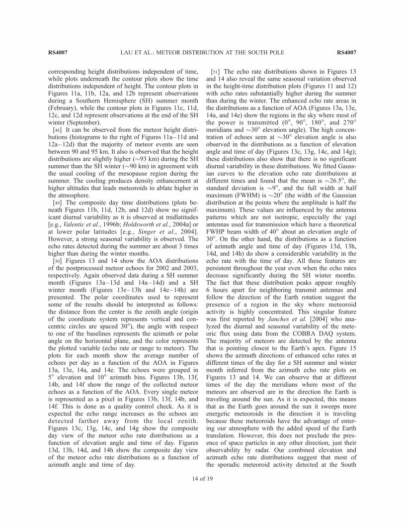
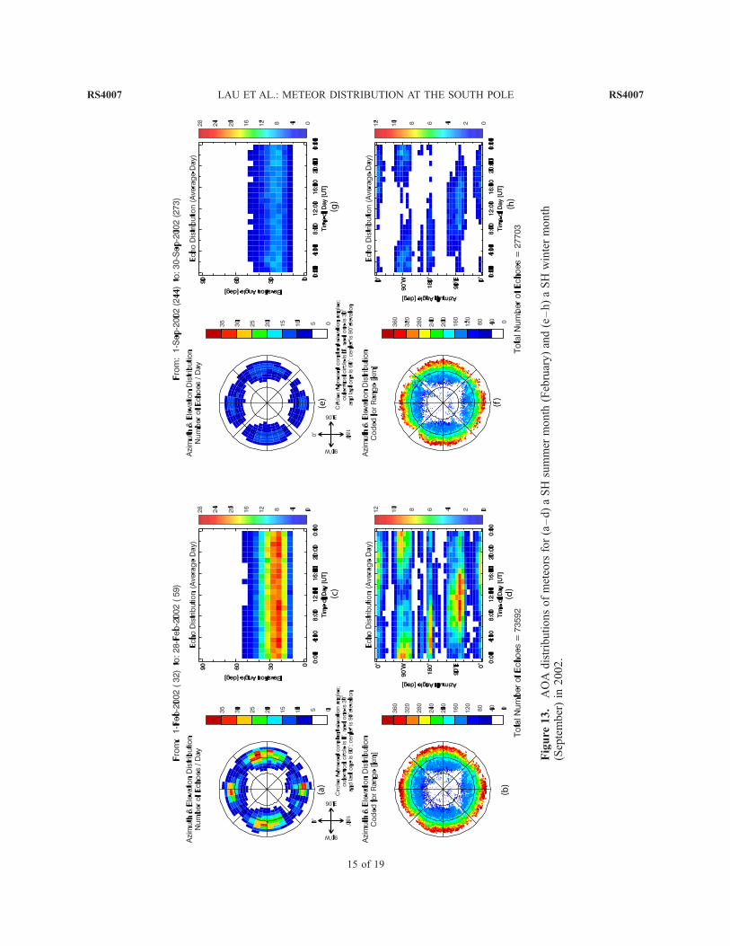
of the postprocessed meteor echoes for 2002 and 2003,respectively. Again observed data during a SH summermonth (Figures 13a–13d and 14a–14d) and a SHwinter month (Figures 13e–13h and 14e–14h) arepresented. The polar coordinates used to representsome of the results should be interpreted as follows:the distance from the center is the zenith angle (originof the coordinate system represents vertical and con-centric circles are spaced 30�), the angle with respectto one of the baselines represents the azimuth or polarangle on the horizontal plane, and the color representsthe plotted variable (echo rate or range to meteor). Theplots for each month show the average number ofechoes per day as a function of the AOA in Figures13a, 13e, 14a, and 14e. The echoes were grouped in5� elevation and 10� azimuth bins. Figures 13b, 13f,14b, and 14f show the range of the collected meteorechoes as a function of the AOA. Every single meteoris represented as a pixel in Figures 13b, 13f, 14b, and14f. This is done as a quality control check. As it isexpected the echo range increases as the echoes aredetected farther away from the local zenith.Figures 13c, 13g, 14c, and 14g show the compositeday view of the meteor echo rate distributions as afunction of elevation angle and time of day. Figures13d, 13h, 14d, and 14h show the composite day viewof the meteor echo rate distributions as a function ofazimuth angle and time of day.

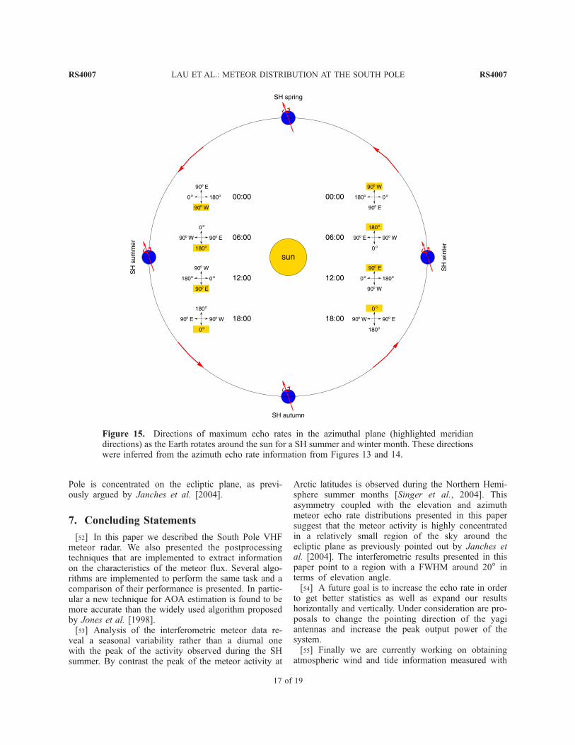
[51] The echo rate distributions shown in Figures 13and 14 also reveal the same seasonal variation observedin the height-time distribution plots (Figures 11 and 12)with echo rates substantially higher during the summerthan during the winter. The enhanced echo rate areas inthe distributions as a function of AOA (Figures 13a, 13e,14a, and 14e) show the regions in the sky where most ofthe power is transmitted (0�, 90�, 180�, and 270�meridians and �30� elevation angle). The high concen-tration of echoes seen at �30� elevation angle is alsoobserved in the distributions as a function of elevationangle and time of day (Figures 13c, 13g, 14c, and 14g);these distributions also show that there is no significantdiurnal variability in these distributions. We fitted Gauss-ian curves to the elevation echo rate distributions atdifferent times and found that the mean is �26.5�, thestandard deviation is �9�, and the full width at halfmaximum (FWHM) is �20� (the width of the Gaussiandistribution at the points where the amplitude is half themaximum). These values are influenced by the antennapatterns which are not isotropic, especially the yagiantennas used for transmission which have a theoreticalFWHP beam width of 40� about an elevation angle of30�. On the other hand, the distributions as a functionof azimuth angle and time of day (Figures 13d, 13h,14d, and 14h) do show a considerable variability in theecho rate with the time of day. All these features arepersistent throughout the year even when the echo ratesdecrease significantly during the SH winter months.The fact that these distribution peaks appear roughly6 hours apart for neighboring transmit antennas andfollow the direction of the Earth rotation suggest thepresence of a region in the sky where meteoroidactivity is highly concentrated. This singular featurewas first reported by Janches et al. [2004] who ana-lyzed the diurnal and seasonal variability of the mete-oric flux using data from the COBRA DAQ system.The majority of meteors are detected by the antennathat is pointing closest to the Earth’s apex. Figure 15shows the azimuth directions of enhanced echo rates atdifferent times of the day for a SH summer and wintermonth inferred from the azimuth echo rate plots onFigures 13 and 14. We can observe that at differenttimes of the day the meridians where most of themeteors are observed are in the direction the Earth istraveling around the sun. As it is expected, this meansthat as the Earth goes around the sun it sweeps moreenergetic meteoroids in the direction it is travelingbecause these meteoroids have the advantage of enter-ing our atmosphere with the added speed of the Earthtranslation. However, this does not preclude the pres-ence of space particles in any other direction, just theirobservability by radar. Our combined elevation andazimuth echo rate distributions suggest that most ofthe sporadic meteoroid activity detected at the South


14 of 19

RS4007

Figure

13.

AOA

distributionsofmeteorsfor(a–d)aSH

summer

month

(February)and(e–h)aSH

wintermonth

(September)in

2002.


15 of 19

RS4007

Figure

14.

Asin

Figure

13butforyear2003.


16 of 19

RS4007

Pole is concentrated on the ecliptic plane, as previ-ously argued by Janches et al. [2004].

7. Concluding Statements

[52] In this paper we described the South Pole VHFmeteor radar. We also presented the postprocessingtechniques that are implemented to extract informationon the characteristics of the meteor flux. Several algo-rithms are implemented to perform the same task and acomparison of their performance is presented. In partic-ular a new technique for AOA estimation is found to bemore accurate than the widely used algorithm proposedby Jones et al. [1998].[53] Analysis of the interferometric meteor data re-

veal a seasonal variability rather than a diurnal onewith the peak of the activity observed during the SHsummer. By contrast the peak of the meteor activity at

Arctic latitudes is observed during the Northern Hemi-sphere summer months [Singer et al., 2004]. Thisasymmetry coupled with the elevation and azimuthmeteor echo rate distributions presented in this papersuggest that the meteor activity is highly concentratedin a relatively small region of the sky around theecliptic plane as previously pointed out by Janches etal. [2004]. The interferometric results presented in thispaper point to a region with a FWHM around 20� interms of elevation angle.[54] A future goal is to increase the echo rate in order

to get better statistics as well as expand our resultshorizontally and vertically. Under consideration are pro-posals to change the pointing direction of the yagiantennas and increase the peak output power of thesystem.[55] Finally we are currently working on obtaining

atmospheric wind and tide information measured with

Figure 15. Directions of maximum echo rates in the azimuthal plane (highlighted meridiandirections) as the Earth rotates around the sun for a SH summer and winter month. These directionswere inferred from the azimuth echo rate information from Figures 13 and 14.


17 of 19

RS4007

the radar system and the results will be published in afuture paper.

Appendix A: Meteor Height Calculation

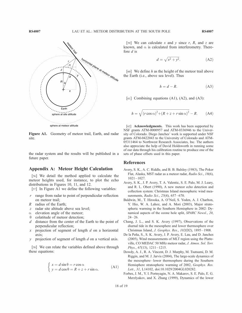
[56] We detail the method applied to calculate themeteor heights used, for instance, to plot the echodistributions in Figures 10, 11, and 12.[57] In Figure A1 we define the following variables:

r range from radar to point of perpendicular reflectionon meteor trail;

R radius of the Earth;z radar site altitude above sea level;a elevation angle of the meteor;q colatitude of meteor detection;d distance from the center of the Earth to the point of

perpendicular reflection;x projection of segment of length d on a horizontal

axis;y projection of segment of length d on a vertical axis.

[58] We can relate the variables defined above throughthese equations:

x ¼ d sin q ¼ r cosay ¼ d cos q ¼ Rþ zþ r sina:

�ðA1Þ

[59] We can calculate x and y since r, R, and z areknown, and a is calculated from interferometry. There-fore d is

d ¼ffiffiffiffiffiffiffiffiffiffiffiffiffiffix2 þ y2

p: ðA2Þ

[60] We define h as the height of the meteor trail abovethe Earth (i.e., above sea level). Thus

h ¼ d � R: ðA3Þ

[61] Combining equations (A1), (A2), and (A3):

h ¼ffiffiffiffiffiffiffiffiffiffiffiffiffiffiffiffiffiffiffiffiffiffiffiffiffiffiffiffiffiffiffiffiffiffiffiffiffiffiffiffiffiffiffiffiffiffiffiffiffiffiffiffiffiffiffiffiffir cosað Þ2þ Rþ zþ r sinað Þ2

q� R: ðA4Þ

[62] Acknowledgments. This work has been supported byNSF grants ATM-0000957 and ATM-0336946 to the Univer-sity of Colorado. Diego Janches’ work is supported under NSFgrants ATM-0422043 to the University of Colorado and ATM-05311464 to Northwest Research Associates, Inc. The authorsalso appreciate the help of David Holdsworth in running someof our data through his calibration routine to produce one of thesets of phase offsets used in this paper.

References

Avery, S. K., A. C. Riddle, and B. B. Balsley (1983), The Poker

Flat, Alaska, MST radar as a meteor radar, Radio Sci., 18(6),

1021–1027.

Avery, S. K., J. P. Avery, T. A. Valentic, S. E. Palo, M. J. Leary,

and R. L. Obert (1990), A new meteor echo detection and

collection system: Christmas Island mesospheric wind mea-

surements, Radio Sci., 25(4), 657–670.

Baldwin, M., T. Hirooka, A. O’Neil, S. Yoden, A. J. Charlton,

Y. Hio, W. A. Lahoz, and A. Mori (2003), Major strato-

spheric warming in the Southern Hemisphere in 2002: Dy-

namical aspects of the ozone hole split, SPARC Newsl., 20,

24–26.

Chang, J. L., and S. K. Avery (1997), Observations of the

diurnal tide in the mesosphere and lower thermosphere over

Christmas Island, J. Geophys. Res., 102(D2), 1895–1908.

De la Pena, S., S. K. Avery, J. P. Avery, E. Lau, and D. Janches

(2005), Wind measurements of MLT region using the Platte-

ville, CO MEDAC 50 MHz meteor radar, J. Atmos. Sol. Terr.

Phys., 67(13), 1211–1215.

Dowdy, A. J., R. A. Vincent, D. J. Murphy, M. Tsutsumi, D. M.

Riggin, and M. J. Jarvis (2004), The large-scale dynamics of

the mesosphere– lower thermosphere during the Southern

Hemisphere stratospheric warming of 2002, Geophys. Res.

Lett., 31, L14102, doi:10.1029/2004GL020282.

Forbes, J. M., Y. I. Portnyagin, N. A. Makarov, S. E. Palo, E. G.

Merzlyakov, and X. Zhang (1999), Dynamics of the lower

Figure A1. Geometry of meteor trail, Earth, and radarsite.


18 of 19

RS4007

thermosphere over South Pole from meteor radar wind mea-

surements, Earth Planets Space, 51, 611–620.

Hernandez, G. (2003), Climatology of the upper mesosphere

temperature above South Pole (90�S): Mesospheric cooling

during 2002, Geophys. Res. Lett . , 30(10), 1535,

doi:10.1029/2003GL016887.

Hernandez, G., R.W. Smith, G. J. Fraser, andW. L. Jones (1992),

Large-scale waves in the upper-mesosphere at Antarctic high-

latitudes, Geophys. Res. Lett., 19(13), 1347–1350.

Hernandez, G., G. J. Fraser, and R. W. Smith (1993), Meso-

spheric 12-hour oscillations near South Pole, Antarctica,

Geophys. Res. Lett., 20(17), 1787–1790.

Hernandez, G., J. M. Forbes, R. W. Smith, Y. Portnyagin, J. F.

Booth, and N. Makarov (1996), Simultaneous mesospheric

wind measurements near South Pole by optical and meteor

radar methods, Geophys. Res. Lett., 23(10), 1079–1082.

Holdsworth, D. A., I. M. Reid, and M. A. Cervera (2004a),

Buckland Park all-sky interferometric meteor radar, Radio

Sci., 39, RS5009, doi:10.1029/2003RS003014.

Holdsworth, D. A., M. Tsutsumi, I. M. Reid, T. Nakamura, and

T. Tsuda (2004b), Interferometric meteor radar phase cali-

bration using meteor echoes, Radio Sci., 39, RS5012,

doi:10.1029/2003RS003026.

Janches, D., S. E. Palo, E. M. Lau, S. K. Avery, J. P. Avery,

S. de la Pena, and N. A. Makarov (2004), Diurnal and sea-

sonal variability of the meteoric flux at the South Pole mea-

sured with radars, Geophys. Res. Lett., 31, L20807,

doi:10.1029/2004GL021104.

Jones, J., A. R. Webster, and W. K. Hocking (1998), An im-

proved interferometer design for use with meteor radars,

Radio Sci., 33(1), 55–65.

McKinley, D. W. R. (1961), Meteor Science and Engineering,

McGraw-Hill, New York.

Mitchell, N. J., D. Pancheva, H. R. Middleton, and M. E. Hagan

(2002), Mean winds and tides in the Arctic mesosphere and

lower thermosphere, J. Geophys. Res., 107(A1), 1004,

doi:10.1029/2001JA900127.

Oznovich, I., D. J. McEwen, G. G. Sivjee, and R. L.

Walterscheid (1997), Tidal oscillations of the Arctic upper

mesosphere and lower thermosphere in winter, J. Geophys.

Res., 102(A3), 4511–4520.

Palo, S. E., and S. K. Avery (1993), Mean winds and the

semiannual oscillation in the mesosphere and lower thermo-

sphere at Christmas Island, J. Geophys. Res., 98(D11),

20,385–20,400.

Palo, S. E., and S. K. Avery (1996), Observations of the quasi-

two-day wave in the middle and lower atmosphere over

Christmas Island, J. Geophys. Res., 101(D8), 12,833–12,846.

Palo, S. E., Y. I. Portnyagin, J. M. Forbes, N. A. Makarov, and

E. G. Merzlyakov (1998), Transient eastward-propagating

long-period waves observed over the South Pole, Ann. Geo-

phys., 16, 1486–1500.

Portnyagin, Y. I., J. M. Forbes, and N. A. Makarov (1997),

Unusual characteristics of lower thermosphere prevailing

winds at South Pole, Geophys. Res. Lett., 24(1), 81–84.

Portnyagin, Y. I., J.M. Forbes, N. A.Makarov, E. G.Merzlyakov,

and S. E. Palo (1998), The summertime 12-h wind oscillation

with zonal wavenumber s = 1 in the lower thermosphere

over the South Pole, Ann. Geophys., 16, 828–837.

Singer, W., J. Weiß, and U. von Zahn (2004), Diurnal and

annual variation of meteor rates at the Arctic Circle, Atmos.

Chem. Phys., 4, 1355–1363.

Stoica, P., and R. L. Moses (1997), Introduction to Spectral

Analysis, Prentice-Hall, Upper Saddle River, N. J.

Strauch, R. G., R. A. Kropfli, W. B. Sweezy, and W. R.

Moninger (1978), Improved Doppler velocity estimates by

the poly-pulse-pair method, paper presented at 18th Confer-

ence on RadarMeteorology, Am.Meteorol. Soc., Atlanta, Ga.

Tabei, M., and B. R. Musicus (1996), A simple estimator for

frequency and decay rate, IEEE Trans. Signal Process.,

44(6), 1504–1511.

Valentic, T. A., J. P. Avery, and S. K. Avery (1996a), MEDAC/

SC: A third generation meteor echo detection and collection

system, IEEE Trans. Geosci. Remote Sens., 34(1), 15–21.

Valentic, T. A., J. P. Avery, S. K. Avery, M. A. Cervera, W. G.

Elford, R. A. Vincent, and I. M. Reid (1996b), A comparison

of meteor radar systems at Buckland Park, Radio Sci., 31(6),

1313–1330.

Valentic, T. A., J. P. Avery, S. K. Avery, and R. A. Vincent

(1997a), A comparison of winds measured by meteor radar

systems and an MF radar at Buckland Park, Radio Sci.,

32(2), 867–874.

Valentic, T. A., J. P. Avery, S. K. Avery, and R. C. Livingston

(1997b), Self-survey calibration of meteor radar antenna ar-

ray, IEEE Trans. Geosci. Remote Sens., 35(3), 524–531.

Wang, S. T., D. Tetenbaum, B. B. Balsley, R. L. Obert, S. K.

Avery, and J. P. Avery (1988), A meteor echo detection and

collection system for use on VHF radars, Radio Sci., 23(1),

46–54.

Younger, P. T., D. Pancheva, H. R. Middleton, and N. J.

Mitchell (2002), The 8-hour tide in the Arctic mesosphere

and lower thermosphere, J. Geophys. Res., 107(A12),

1420, doi:10.1029/2001JA005086.

��S. K. Avery, E. M. Lau, and R. Schafer, Cooperative

Institute for Research in Environmental Sciences, University of

Colorado, 216 UCB, Boulder, CO 80309, USA. (elias.lau@

colorado.edu)

J. P. Avery, Department of Electrical and Computer

Engineering, University of Colorado, 425 UCB, Boulder, CO

80309, USA.

D. Janches, CoRA Division, Northwest Research Associ-

ates, 3380 Mitchell Lane, Boulder, CO 80301, USA.

N. A. Makarov, Institute for Experimental Meteorology,

Scientific Production Association TYPHOON, Obninsk

249020, Russia.

S. E. Palo, Department of Aerospace Engineering, Uni-

versity of Colorado, 429 UCB, Boulder, CO 80309, USA.


19 of 19

RS4007

Documents

Statistical characterization of the meteor trail distribution at the South Pole as seen by a VHF interferometric meteor radar