Food Quality and Preference 21 (2010) 805–814

Contents lists available at ScienceDirect

Food Quality and Preference

journal homepage: www.elsevier .com/locate / foodqual

Statistical inference for temporal dominance of sensations data usingrandomization tests

Michael Meyners a,*, Nicolas Pineau b

a Holzbaumweg 34, Haselünne, Germanyb Nestec SA, Applied Mathematics, Lausanne, Switzerland

a r t i c l e i n f o

Article history:Received 18 June 2009Received in revised form 14 April 2010Accepted 14 April 2010Available online 22 April 2010

Keywords:Temporal dominance of sensations (TDS)Statistical inferenceRandomization testsPermutation tests

0950-3293/$ - see front matter � 2010 Elsevier Ltd. Adoi:10.1016/j.foodqual.2010.04.004

* Corresponding author. Address: Procter & GamInnovation Center, Schwalbach am Taunus, Germany.

E-mail addresses: m.meyners@web.de, meyners.m

a b s t r a c t

Temporal dominance of sensations (TDS) is a relatively new notion to investigate the evolution of dom-inant sensations of a product throughout a pre-defined period like, e.g., mastication or aftertaste. It ismainly used for a description of the characteristics of each single product over time. In contrast, valid sta-tistical inference to compare the products globally or in pairwise comparisons has not yet been devel-oped. We close this gap by introducing a randomization test based on distances between matrices. Forthis purpose, TDS sequences are unfolded to data matrices with a single non-zero entry per time point(column). The sum of the Euclidean distances between these matrices is determined and serves as a teststatistic for the global test. Similar statistics are employed for pairwise comparisons and for inference byattribute or time point. Re-randomizations are used to determine the null distribution and p-values, tak-ing the original restrictions of the randomization into account. We give the details of this procedure andsketch the underlying algorithm to perform the tests. We also propose some simple graphical methods tosummarize the many p-values derived from this approach (usually at least hundreds, but more often sev-eral thousands). We apply this approach to real data and show that it gives reasonable and easily inter-pretable results, complementing existing methods.

� 2010 Elsevier Ltd. All rights reserved.

1. Introduction

Temporal dominance of sensations (TDS) is a recently devel-oped sensory test procedure. Several subjects are asked to judgecontinuously throughout a certain period which out of a few attri-butes (up to 8, say) is the dominant one, and also to rate the inten-sity of the dominant attribute (see, e.g., Labbe, Schlich, Pineau,Gilbert, & Martin, 2009; Pineau et al., 2009 and the referencestherein, in particular also to the so-called grey literature, in whichTDS was first described in 2004). Usually considered periods ofinterest include the mastication period and the aftertaste period.

Up to now, statistical analysis is usually confined to a descrip-tion of the data, the depiction of the average dominance curves,and some rough cut-off limits based on the binomial law to definenoteworthy increased elicitation of any attribute at any point intime. To the best of our knowledge, a profound set of valid statis-tical tests has not yet been proposed.

With this paper, we intend to close this gap and propose anappropriate and valid set of statistical tests that allow investigatingoverall differences as well as differences between pairs of products,and within each framework next to a general test, tests per attri-

ll rights reserved.

ble Service GmbH, GermanTel.: +49 6196 89 3987.

@pg.com (M. Meyners).

bute, per time point and per attribute by time point are suggested.All tests are based on the general notion of randomization tests (cf.Edgington & Onghena, 2007), and they are valid level a tests forthemselves. In contrast, the whole test set with at least severalhundreds of tests does not respect the family-wise significancelevel, and correction for multiplicity might be called for. However,this is not specific to our test, but inherent in the many hypothesesto be tested and will therefore apply to any alternative set of teststhat might ever be developed.

For the sake of simplicity, in the main part of the paper we as-sume that the time periods are standardized across subjects andproducts, such that each observation has a fixed number of timepoints. This assumption implies that the perception of dominancedepends on the overall duration of the period of interest, and thattwo products might get identical dominance rates even though thedurations differ strongly. It depends on the actual experimentwhether this is a reasonable assumption or not, but the introduc-tion of our test is much easier under this assumption. Furthermore,we confine ourselves to the pure choice of attributes and neglectthe intensity scores for the main part of the paper. We will outlinehow our approach can be generalized by means of data preprocess-ing to account for unstandardized data and for the use of the inten-sity scores in Section 11.

The remainder of the manuscript proceeds as follows: we startby illustrating the concept of randomization tests in a very simple

806 M. Meyners, N. Pineau / Food Quality and Preference 21 (2010) 805–814

setting in Section 2. There, we also give some historical notes andrefer to selected applications of permutation tests in the (mainlysensory) literature. This part can safely be skipped by readersfamiliar with the notion. We then introduce the notation inSection 3. We proceed by defining distances and averages of TDSassessments before we describe the appropriate choice of re-randomizations for the simplest settings in Section 5. Next, wedefine the overall test for product differences, and subsequentlySection 7 covers the corresponding tests for pairwise comparisonsat an overall level. In Section 8, we define the appropriate tests atattribute or time point level, and at attribute by time point level.We conclude the technical part by proposing a graphical methodto display the many results obtained in Section 9. Section 10revisits a real data example from the literature to which we applyour approach. It also provides some insight into the possibleinterpretations thereof. We then generalize the approach tounstandardized data (i.e. different number of time points fordifferent assessors or even different assessments of the sameassessor), and we outline how the intensity scores could be usedin our approach as well. Section 12 compares our approach tothe proposals of Pineau et al. (2009). After a brief discussion ofthe difficulty in finding alternative analytical tests in Section 13,we conclude by discussing a few computational issues, summariz-ing the main findings and give some outlook on possible futureresearch.

2. Randomization tests

The concept of randomization testing is essential for theremainder of the paper. For the sake of completeness we brieflyrecapitulate this concept by illustrating it with a simple example.For further details we refer to the textbook by Edgington andOnghena (2007), who also define the difference between random-ization tests and permutation tests, even though these terms arefrequently used as equivalent. Readers who are familiar with ran-domization tests may skip this section.

For illustration purposes, assume five panelists are asked tomonadically rate the sweetness of two products A and B, say. Foreach assessor, we independently randomize the order of the prod-ucts. Assume that the following sequence defines the first productfor each assessor:

A B B A BNote that we do not assume the design to be (nearly) balanced.

Now assume that we observe the following differences betweenthe intensity ratings for A and B:

1 3 3 4 �1

Table 1All possible permutations of the first product served to five assessors with correspondingdifference of two units are set in bold.

Assessor Mean difference

1 2 3 4 5

A A A A A 0.0A A A A B �0.4A A A B A �1.6A A A B B �2.0A A B A A 1.2A A B A B 0.8A A B B A �0.4A A B B B �0.8A B A A A 1.2A B A A B 0.8A B A B A �0.4A B A B B �0.8A B B A A 2.4A B B A B 2.0A B B B A 0.8A B B B B 0.4

Hence the first assessor rated A one point higher than B, the sec-ond three points higher, and so on. On average, A is rated 2 pointshigher than B. We could make some assumptions like, e.g., normal-ity of residuals, and apply a t-test or a non-parametric rank basedtest to these results. However, assume that we know that all theseassumptions are violated for our data. We nevertheless want totest the null hypothesis of product equality against its alternativeof product differences. To do so, we make use of the fact that werandomized the order of products for each panelist.

To start with assessor 1, we observe that he rates A (testedfirst) one point higher than B. However, if the null hypothesisof product equality with regard to sweetness holds true, thisdifference cannot be due to real differences in sweetness, but onlydue to assessor-intrinsic variation like perceptual variation,fatigue, imprecise scoring, etc. In other words, the assessor givesa certain score to the first product which was by chance A here,but he would have given exactly the same score if the producthad been B. The same holds for the second product tested. So ifhe had obtained product B first and then A, the above differencein intensity ratings would have been �1 instead of 1. The meandifference would have been 1.6 only in that case. The samereasoning holds for every assessor as, under the null hypothesis,there is no difference in sweetness. In total, there are 25 = 32different sequences defining the first product to be served tothe five assessors. All of these have been equally likely to bechosen when the experiment was designed, as for each assessorwe randomly, independently and with equal probability selectedone of the two products to be served first.

The 32 possible sequences are listed in Table 1 together withthe corresponding mean difference between the groups. It is foundthat e.g., the sequence BABBA, yields a mean difference of �0.8,while, of course, the opposite of the initial sequence, i.e. BAABAgives a mean difference of �2. If the observed (absolute) mean dif-ference is large compared to the values obtained by all re-random-izations, we conclude that this is unlikely due to chance only, andthat there is hence a difference in sweetness. For our data, 3 of the32 re-randomizations (9.4%) yield a mean difference of 2 or larger,and due to symmetry, the same proportion yields a mean differ-ence equal to �2 or smaller. From a one-sided test, we wouldhence conclude that A is sweeter than B at the 10% level, whilethe two-sided tests fails to prove a difference even at level 10%,as the corresponding p-value is 6/32 = 0.1875.

It is generally important to note that only admissible random-izations should be considered, i.e. randomizations that could havebeen chosen for the real experiment as well. If, e.g., the productorder had to be as balanced as possible, many of the sequences

mean differences between groups. Absolute values at least as large as the observed

Assessor Mean difference

1 2 3 4 5

B A A A A �0.4B A A A B �0.8B A A B A �2.0B A A B B �2.4B A B A A 0.8B A B A B 0.4B A B B A �0.8B A B B B �1.2B B A A A 0.8B B A A B 0.4B B A B A �0.8B B A B B �1.2B B B A A 2.0B B B A B 1.6B B B B A 0.4B B B B B 0.0

M. Meyners, N. Pineau / Food Quality and Preference 21 (2010) 805–814 807

would not have been admissible. Only sequences with either 2 or 3.As could have been used, reducing the number of sequences to 20in our case. Also any other restrictions like, e.g., reversing the orderfor every panelist in a second replication, have to be taken into ac-count. Otherwise, like inappropriate classical tests, the randomiza-tion test may give seriously misleading results.

In more complex situations or with larger data sets, it might beimpractical or even impossible to consider all possible randomiza-tions. Instead, numerous draws from all admissible randomizationscan be used to approximate the exact p-values. Usually 1000 or10,000 draws will give sufficient accuracy. In theory, samplingshould be done without replacement. However, if the number ofsamples is relatively small compared to the number of possible ran-domizations, sampling with replacement will usually give the sameresults and might be preferred for computational performance. Itshould be noted that the randomization actually used in the exper-iment itself should be considered as one of the draws. If not, the de-rived p-value is liberal (see Edgington and Onghena (2007) fordetails).

It should also be noted that common parametric and non-para-metric tests can be thought of as randomization tests. For normallydistributed data, the t-test and the corresponding randomizationtest will give the same results. Again, in more complex situationsas an ANOVA, it is important to respect the structure of the design(blocking, nesting) for the randomization test. If this is done, thetest will give the same result as the appropriate F-tests if the dataare truly normally distributed.

Historically, the notion of randomization tests goes back to theearly 20th century (Eden & Yates, 1933; Fisher, 1935; Pitman,1937a, 1937b; Pitman, 1938; see also David (2008)). Some authorsconsider randomization tests even generally superior to paramet-ric alternatives in certain areas (Ludbrook & Dudley, 1998). Wehave applied randomization tests successfully in many differentsituations, a few of which have been published elsewhere(Meyners, 2001; Meyners & Arndt, 2005). Several authors appliedpermutation tests to sensory or consumer studies. Dijksterhuisand Heiser (1995) described them as a general alternative to clas-sical methods in multivariate data analysis. Wakeling, Raats, andMacFie (1992) derived a test for consensus in generalized procrus-tes analysis (GPA), which was extended by Wu, Guo, de Jong, andMassart (2002) to determine the appropriate dimensionality ofthe consensus. Xiong, Blot, Meullenet, and Dessirier (2008) proposeanother, model-based variation of this test. Recently, Bi (2009) pro-posed the use of randomization tests (among others) for Durbin’srank test. This list is not exhaustive, but already indicates thatthere are many different applications in sensory sciences whichmight benefit from the use of randomization tests.

3. Notation

Throughout this paper, we assume that a TDS experiment hasbeen performed by judges j = 1, . . ., nJ in replications s = 1, . . ., nS

on products p = 1, . . ., nP using attributes a = 1, . . ., nA. Furthermore,we assume that the time period for each single experiment by

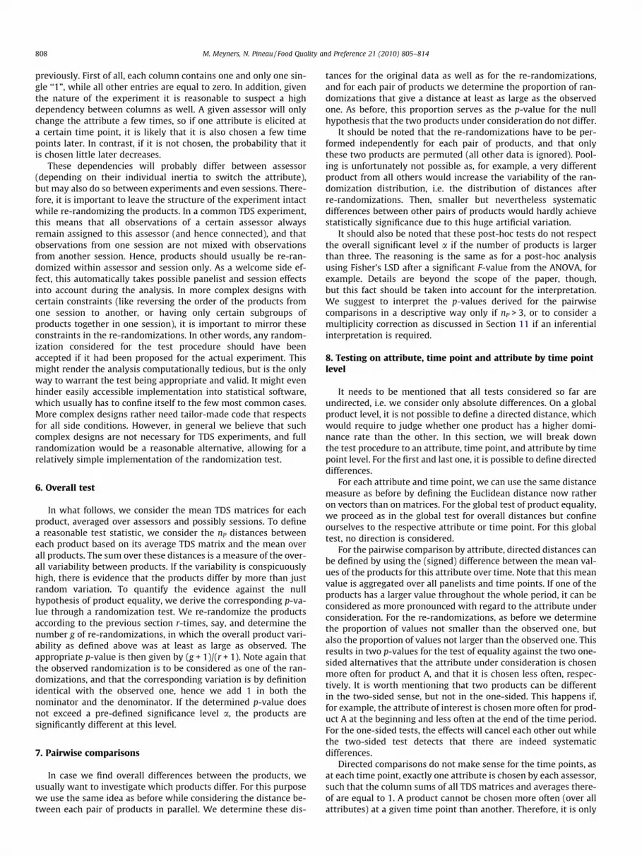
poin0 4 8

meltingharddry

crunchycrispy 0 0 0 0 0 0 0 1 1 1

0 0 0 0 0 0 0 0 0 00 0 0 0 0 0 0 0 0 01 1 1 1 1 1 1 0 0 00 0 0 0 0 0 0 0 0 0

hard crisp

Fig. 1. Artificial sequence of dominant attributes for one ass

judge, session and product is subdivided into time points t = 1,. . ., nT. Capital letters like X and Y indicate matrices, and {X}kl givesthe entry of matrix X in row k and column l. As indicated in theintroduction, for the main part of the paper we particularly assumenT to be fixed for all evaluations.

4. Distances and averages for TDS assessments

A consolidated and comprehensive depiction of a single TDS testby one assessor on one product is the sequence of attributes cho-sen over time like, e.g., given in the lower part of Fig. 1. However,it seems difficult to define a reasonable distance between two suchsequences based on this format, and even less an average of severalsequences. Therefore, we propose to unfold the sequences intomatrices Xjp � (nA � nT), i.e. one row for each attribute a and onecolumn for each time point t, for each judge j and product p (andpossibly replication s, which is omitted here from the notationfor brevity). For these matrices, {Xjp}at = 1 if and only if attributea was chosen by judge j on product p at time point t, and 0 other-wise. Hence, there is exactly one ‘‘1” in each column, while allother entries are zero, as just one single attribute can and has tobe chosen at any time. The respective data matrix is also given inFig. 1. Note that dry has not been elicited in this artificial example,and does hence not occur in the sequence.

For these matrices, it is straightforward to define distances be-tween them, for example using the Lk-norms for any integer k. Themost common choice is k = 2, resulting in the Euclidean distance,which relates to the least squares criterion frequently used in sta-tistical inference. Without loss of generality, we confine ourselvesto the L2-norm in what follows, while any other distance measurecould be used instead, as outlined in Section 11.

The squared Euclidean distance between two equally sizedmatrices X and Y is defined by jjX � Yjj2 ¼

Pk;lðfX � YgklÞ

2, k and lvarying over the rows and columns of the difference matrix,respectively. For our purposes, using the squared Euclidean dis-tance or the distance itself (i.e. the square root of the former) isequivalent due to the square root being a strictly monotone trans-formation. For simplicity and most efficient computations, we willbase our test on the squared Euclidean distance. Note that in caseof comparing just two individual sequences, the squared Euclideandistance is identical to twice the number of time points for whichdifferent attributes were dominant. For averages of sequences asused here, this simple interpretation does not apply, though.

Next to the distances, averages over different equally sizedmatrices are defined by averaging the matrices element-wise.

For investigations by attribute or by time point, we consider theresulting vectors as matrices of dimension (nA � 1) and (1 � nT),respectively, and for investigations by attribute and time point,the real scalars are considered as matrices of dimension (1 � 1).

5. Choice of appropriate re-randomizations

It is important to notice that there is a high dependencybetween the data points in a single TDS data matrix as defined

t in time12 16 20

1 1 0 0 0 0 0 0 0 0 00 0 1 1 1 0 0 0 0 0 00 0 0 0 0 0 0 0 0 0 00 0 0 0 0 0 0 0 1 1 10 0 0 0 0 1 1 1 0 0 0y crunchy melting hard

essor and one product with corresponding data matrix.

808 M. Meyners, N. Pineau / Food Quality and Preference 21 (2010) 805–814

previously. First of all, each column contains one and only one sin-gle ‘‘1”, while all other entries are equal to zero. In addition, giventhe nature of the experiment it is reasonable to suspect a highdependency between columns as well. A given assessor will onlychange the attribute a few times, so if one attribute is elicited ata certain time point, it is likely that it is also chosen a few timepoints later. In contrast, if it is not chosen, the probability that itis chosen little later decreases.

These dependencies will probably differ between assessor(depending on their individual inertia to switch the attribute),but may also do so between experiments and even sessions. There-fore, it is important to leave the structure of the experiment intactwhile re-randomizing the products. In a common TDS experiment,this means that all observations of a certain assessor alwaysremain assigned to this assessor (and hence connected), and thatobservations from one session are not mixed with observationsfrom another session. Hence, products should usually be re-ran-domized within assessor and session only. As a welcome side ef-fect, this automatically takes possible panelist and session effectsinto account during the analysis. In more complex designs withcertain constraints (like reversing the order of the products fromone session to another, or having only certain subgroups ofproducts together in one session), it is important to mirror theseconstraints in the re-randomizations. In other words, any random-ization considered for the test procedure should have beenaccepted if it had been proposed for the actual experiment. Thismight render the analysis computationally tedious, but is the onlyway to warrant the test being appropriate and valid. It might evenhinder easily accessible implementation into statistical software,which usually has to confine itself to the few most common cases.More complex designs rather need tailor-made code that respectsfor all side conditions. However, in general we believe that suchcomplex designs are not necessary for TDS experiments, and fullrandomization would be a reasonable alternative, allowing for arelatively simple implementation of the randomization test.

6. Overall test

In what follows, we consider the mean TDS matrices for eachproduct, averaged over assessors and possibly sessions. To definea reasonable test statistic, we consider the nP distances betweeneach product based on its average TDS matrix and the mean overall products. The sum over these distances is a measure of the over-all variability between products. If the variability is conspicuouslyhigh, there is evidence that the products differ by more than justrandom variation. To quantify the evidence against the nullhypothesis of product equality, we derive the corresponding p-va-lue through a randomization test. We re-randomize the productsaccording to the previous section r-times, say, and determine thenumber g of re-randomizations, in which the overall product vari-ability as defined above was at least as large as observed. Theappropriate p-value is then given by (g + 1)/(r + 1). Note again thatthe observed randomization is to be considered as one of the ran-domizations, and that the corresponding variation is by definitionidentical with the observed one, hence we add 1 in both thenominator and the denominator. If the determined p-value doesnot exceed a pre-defined significance level a, the products aresignificantly different at this level.

7. Pairwise comparisons

In case we find overall differences between the products, weusually want to investigate which products differ. For this purposewe use the same idea as before while considering the distance be-tween each pair of products in parallel. We determine these dis-

tances for the original data as well as for the re-randomizations,and for each pair of products we determine the proportion of ran-domizations that give a distance at least as large as the observedone. As before, this proportion serves as the p-value for the nullhypothesis that the two products under consideration do not differ.

It should be noted that the re-randomizations have to be per-formed independently for each pair of products, and that onlythese two products are permuted (all other data is ignored). Pool-ing is unfortunately not possible as, for example, a very differentproduct from all others would increase the variability of the ran-domization distribution, i.e. the distribution of distances afterre-randomizations. Then, smaller but nevertheless systematicdifferences between other pairs of products would hardly achievestatistically significance due to this huge artificial variation.

It should also be noted that these post-hoc tests do not respectthe overall significant level a if the number of products is largerthan three. The reasoning is the same as for a post-hoc analysisusing Fisher’s LSD after a significant F-value from the ANOVA, forexample. Details are beyond the scope of the paper, though,but this fact should be taken into account for the interpretation.We suggest to interpret the p-values derived for the pairwisecomparisons in a descriptive way only if nP > 3, or to consider amultiplicity correction as discussed in Section 11 if an inferentialinterpretation is required.

8. Testing on attribute, time point and attribute by time pointlevel

It needs to be mentioned that all tests considered so far areundirected, i.e. we consider only absolute differences. On a globalproduct level, it is not possible to define a directed distance, whichwould require to judge whether one product has a higher domi-nance rate than the other. In this section, we will break downthe test procedure to an attribute, time point, and attribute by timepoint level. For the first and last one, it is possible to define directeddifferences.

For each attribute and time point, we can use the same distancemeasure as before by defining the Euclidean distance now ratheron vectors than on matrices. For the global test of product equality,we proceed as in the global test for overall distances but confineourselves to the respective attribute or time point. For this globaltest, no direction is considered.

For the pairwise comparison by attribute, directed distances canbe defined by using the (signed) difference between the mean val-ues of the products for this attribute over time. Note that this meanvalue is aggregated over all panelists and time points. If one of theproducts has a larger value throughout the whole period, it can beconsidered as more pronounced with regard to the attribute underconsideration. For the re-randomizations, as before we determinethe proportion of values not smaller than the observed one, butalso the proportion of values not larger than the observed one. Thisresults in two p-values for the test of equality against the two one-sided alternatives that the attribute under consideration is chosenmore often for product A, and that it is chosen less often, respec-tively. It is worth mentioning that two products can be differentin the two-sided sense, but not in the one-sided. This happens if,for example, the attribute of interest is chosen more often for prod-uct A at the beginning and less often at the end of the time period.For the one-sided tests, the effects will cancel each other out whilethe two-sided test detects that there are indeed systematicdifferences.

Directed comparisons do not make sense for the time points, asat each time point, exactly one attribute is chosen by each assessor,such that the column sums of all TDS matrices and averages there-of are equal to 1. A product cannot be chosen more often (over allattributes) at a given time point than another. Therefore, it is only

M. Meyners, N. Pineau / Food Quality and Preference 21 (2010) 805–814 809

possible to investigate whether two products differ at all at a cer-tain time point, not in which direction.

Finally, if we look at each time point by attribute, there is only asingle value for each product, and we can directly determine thedifference on this time point by attribute combination betweentwo products. Squaring this difference results in an undirected test,while taking the original signed values into account allows for di-rected tests as defined above for attributes. In this case, the two-sided p-value from the undirected test can never fall below thesmaller one of the two one-sided p-values from the directed tests.As we usually want an interpretation of the direction, it is usuallyreasonable to consider the one-sided tests only, employing a signif-icance level of a/2 instead of a.

9. Summarizing and interpreting results

In the preceding sections, several tests have been proposed toinvestigate the difference between the products either on a globallevel or for pairs of products. There is an implicit hierarchy forsome of the tests (e.g., global tests followed by pairwise compari-sons), but not for all of them (e.g., attributes are considered in par-allel to time points). Formal testing would hence need to accountfor this as well as for the fact that the pairwise comparisons needto be performed at an adjusted level even after a significant globaltest. We consider the TDS methodology as a rather descriptive toolby construction, and we therefore prefer to perform all tests atlevel a (the one-sided tests possibly at level a/2) and interpret allresults in a descriptive way only. We propose that usually onlythe global test on overall product differences is considered as aformal statistical test. Nevertheless, note that all the proposed testsare valid and respect the nominal level a. Only if used together,they will not keep the family-wise error rate anymore. Multiplicitycorrections are briefly discussed in Section 11.

Even in a small TDS study, the total number of tests can be veryhigh if all of the proposed tests are performed. Assume a studywith just nP = 3 products, nT = 50 time points, and nA = 5 attributes.Next to the 56 overall tests (globally, by attribute, and by timepoint), there are three pairwise comparisons. For each of these,the same tests (56) plus the tests by time point and attribute(50 � 5) are performed. In total, even for this relatively small study,we hence have 974 tests, underlining the impossibility to considerall of them in an inferential way. At the same time, this huge num-ber of tests raises the question how the results can be presented inan easily digestible way.

As mentioned earlier, there is a strong dependency between theindividual data (by product, attribute and time point), and there-fore there is as well between the test results. We propose to sum-marize the results for each pairwise comparison in a figure withtime points in chronological order given on the horizontal axis,and attributes on the vertical axis. At each location defined by atime point and an attribute, a colored dot indicates that product1 has a higher dominance rate than product 2, a differently coloreddot indicates that it is the other way round, and no dot indicatesthat no difference at the chosen threshold was found. In addition,attribute names can be colored the same way if product 1 has high-er or lower dominance rates than product 2, respectively. A thirdcolor is needed to indicate that there were indeed differences,but in different directions, which cancel each other out for theone-sided tests, see above. An additional row can be added to indi-cate whether the differences at a certain time point between theproducts were larger than the threshold. As this is an undirectedtest, coloring is not needed and simple absence or presence of a(black) dot can indicate this. Finally, the plot title can also be col-ored to indicate whether the two products were found differentat all. For the global tests on all products, no similar graphical rep-resentation seems necessary as the number of p-values is limited

to nA + 1 if we ignore the global test by time point, which seemsof least interest in most applications. Of course, different variationsof this approach are possible, but the general idea of illustratingthe numerous results in a consolidated graphic has proven usefulto us. An example is given in the next section.

10. Example

Lenfant, Loret, Pineau, Hartmann, and Martin (2009) collectedTDS data on the mastication of six types of wheat flakes (WF A,B, C, D, E, and F, respectively) that differed in thickness and toastinglevel only while not in composition. Twenty-four panelists com-pleted two TDS sessions with all products, while two additionalpanelists completed a single session. In total, there are hence 50evaluations available per product. The attributes considered werebrittleness, crispiness, crunchiness, dryness, grittiness, hardness, melt-ing, and stickiness. We consider the standardized data by splittingeach mastication period into 100 intervals of equal length. Thuswe have nT = 101 equally spaced time points (including time zero).

The order of products was randomized according to the follow-ing scheme: The same basic Latin square for six products was usednine times, but with different, randomly selected assignments ofthe products to the levels of the original Latin square. The 50 eval-uations were independently randomized to the rows of the eightfirst Latin squares and two randomly selected rows from the lastLatin square. In total, with 6! = 720 possible orderings of the sixproducts and eight independent assignments to the Latin squares,there are 7208 possible randomizations for the first 48 productorders. For the remaining two, there are 1800 different possibilitiesto randomly choose two of six rows of the Latin square and assign-ing the products to these (note that this is much less than

62

� �� 720 as many combinations will yield the same product or-

ders). In total, there are hence about 1026 possible permutations.We used the same procedure to draw 10,000 re-randomizationsfrom this scheme. For the pairwise comparisons, the randomiza-tion scheme implied a balance in the ordering of the two productsunder consideration across 48 samples. The remaining two ordersare drawn from the four possibilities with probability 2/10 forusing P1 first twice, 2/10 for using P2 first twice, and 6/10 for test-ing each product first once (these probabilities are derived fromthe original sampling scheme). The orderings are randomly as-

signed to the assessors. In total, there are 5025

� �� 1014 possible

randomizations with slight differences in their probabilities to bechosen (due to the last 2 orders). Again 10,000 randomizationswere drawn from this sampling scheme for each pair of products.Note that in all cases, the original assignment was considered asone of the re-randomizations.

As the number of samples is tiny compared to the number ofpossible randomizations, and as sampling without replacementwould have been computationally much more cumbersome, sam-pling was performed with replacement. Chances that at least onerandomization has been chosen in duplicate are negligible, though(about 7.5 � 10�6 for all tests simultaneously).

All calculations were performed in R 2.8.1 (R Development CoreTeam, 2008). Computation time for 10,000 re-randomizations eachwas about 6 h on a PC with 2.33 GHz and 2 GB RAM. In applica-tions, usually 1000 re-randomizations will suffice, taking about35 min for an experiment of this dimension on a similar machine.The R code for the example is available upon request from theauthors.

Table 2 gives the p-values for the global test of product differ-ences, considering all attributes either simultaneously or in paral-lel. It is found that we can indeed statistically prove that there are

Table 2Overall p-values from the analysis of TDS data on six wheat flakes (global test and byattribute; significant p-values at level 5% are set in bold).

Attribute p-Value

(Overall) 0.0001Brittleness 0.0001Crispiness 0.0001Crunchiness 0.0001Dryness 0.4013Grittiness 0.0001Hardness 0.0001Melting 0.0001Stickiness 0.5765

810 M. Meyners, N. Pineau / Food Quality and Preference 21 (2010) 805–814

differences between the products in the TDS evaluations, and thatthese manifest themselves in all attributes but dryness and sticki-ness. For the latter, there is no evidence at all to be differentiallyelicited between products. Note that 0.0001 is the smallest possi-ble p-value with 10,000 randomizations.

It should be noted that all subsequent evaluations are consid-ered as descriptive only, even though we apply a statistical signif-icance level of 5% throughout for both the one and the two-sidedcomparisons. However, due to multiplicity, the overall significancelevel is not respected. For simplicity, in what follows we will nev-ertheless use the ‘‘significance” terminology, bearing in mind thatstatistical significance in this sense rather indicates a possible dif-ference than proving it.

Fig. 2 shows the results of all pairwise comparisons between theproducts. A black figure title indicates that the products were sig-nificantly different at the 5% level. In contrast, a grey title indicatesthat there was no evidence of differences between the two prod-ucts under consideration. Furthermore, a red bar or attribute (inthe electronic version; the color is light grey in the printed version)indicates that the dominance rate for the respective attribute washigher for the first product than for the second at this point in time.A blue (dark grey) bar or attribute name indicates the reverse.White spaces and black attribute names indicate no differences,respectively. Green (medium grey) attribute names indicate thatthere were differences between the two products under consider-ation, but these did not occur systematically in one direction. Thelast row of each figure indicates whether (black) or not (white)there was an overall difference between the products across attri-butes at the corresponding time point.

As a general finding, the pairs A–F, C–D and E–F do not showsignificant differences. In addition, the overall test between Aand E has the largest p-value among those significant, indicatingthat these products are less different than most other pairs. Thisis in line with the interpretation of Lenfant et al. (2009), groupingA, E, and F together as well as C and D, with B being different fromboth groups. It is seen that for B, dominance rates for brittleness,crispiness, and crunchiness are lower than for the other products,in particular than those from the first group (A, E, F). In contrast,dominance rates are higher on grittiness and hardness. Comparedto C and D, products A, E, and F show lower dominance rates onmelting and to some extent on brittleness and crispiness at thebeginning of the mastication period. The rates are higher on hard-ness and crunchiness as well as on grittiness towards the end of themastication period. The comparison between products C, D and Fshow that dominance rates for the former two on crispiness arehigher at the beginning of the mastication period, while they arelower on this attribute at about the mean of the mastication peri-od. The same holds for the comparison between D and E. This is atypical example for attribute names appearing in green (mediumgrey), as neither product has higher dominance rates on this attri-bute throughout the time, but there is a clear evolution over timewith differences between the products.

It should be noted that we do not investigate the general evolu-tion of certain attributes over time as Lenfant et al. (2009) did,reporting for instance that dominance rates for all products werehigher on hardness in the beginning than towards the end of themastication period. Instead we focus on the differences betweenproducts only, which might manifest themselves even at relativelylow overall dominance rates. From the results given in Fig. 2, it ispossible to recover some of the interpretation given by Lenfantet al. (2009), while it is mainly complementary. Product B, forexample, has higher rates for hardness and grittiness, while the lat-ter is found mainly in the mean and late part of the masticationperiod. From this, we can indirectly conclude that B is perceivedas hard and then gritty, as Lenfant et al. (2009) do. However, B isperceived harder than all the other products throughout the masti-cation period. So even if the absolute dominance rate of this attri-bute is low towards the end, hardness nevertheless discriminatesbetween the products. In contrast, Lenfant et al. (2009) report thatstickiness becomes the dominant attribute for all samples at theend of the mastication period. Our analysis reveals that there arehardly any differences between the products with regard to thedominance of stickiness; it is in fact the least discriminating of allattributes and can hardly serve to differentiate between products.Stickiness at the end of the mastication period can hence be consid-ered as a general property common to all samples. It does not dis-criminate between them, though, at least not within the notion ofdominance. Of course there might be differences in perceivedintensity of stickiness; this is not addressed by the current analysis.

11. Generalizations and extensions

In our example, we have chosen 101 time points for each indi-vidual time period. It is worth mentioning that this number is com-pletely arbitrary, though. Generally, the number of time pointsshould not be chosen too small, as this would make the intervalsfor (some) panelists too large, and we might miss some differencesbetween products that occur in between. Three or four time pointswill hence not suffice in almost any application. A too large num-ber will increase the computational burden, though it will not havea major impact on the results, as the correlation between neigh-bored observations will increase. A reasonable choice depends onthe absolute duration of the mastication and on the rate by whichthe assessors are changing the attributes. We believe that one datapoint per second (for the longest absolute period) should usuallysuffice, while for long mastication periods with relatively rarechanges, we might want to use even less. For our example, the101 time points were probably already more than necessary, asthe mastication period did not exceed about 40 s. The numberwas mainly chosen in order to match prior analyses of the samedata.

So far, we have confined our considerations to standardizedelicitation data, i.e. the periods were standardized to the sameinterval length (101 time points in our example), and to the numberof elicitations per attribute, ignoring any intensity scores given.However, some practitioners prefer to use the intensity scores orleave the time intervals unstandardized. In what follows, we out-line some modifications to allow for these generalizations of ourapproach. It is beyond the scope of this paper to discuss the prosand cons of standardization and of using intensity scores, respec-tively. Instead, we confine ourselves to describe some data prepro-cessing that allows the usage of the randomization test as describedin this paper. In addition, we will briefly address the use of differentdistance measures as well as the problem of multiplicity.

To start with, we drop the assumption that the data is standard-ized to a certain period length. As the duration can (and will) varybetween products, assessors and replications, this implies a differ-ent number of time points for each evaluation. A straightforward

Fig. 2. Graphical visualization of randomization test results for all pairwise comparisons. Titles in black indicate statistically significant differences between the productsunder consideration. Red bars and attribute names (online; light grey in printed version) indicate higher dominance rates for the first product, blue (dark grey) ones higherrates for the second product, and green (medium grey) ones general, but not systematically directed differences. Overall differences at a given time point are indicated by ablack bar. Significance level is 5%, while no correction for multiplicity was applied. (For interpretation of the references to color in this figure legend, the reader is referred tothe web version of this article.)

M. Meyners, N. Pineau / Food Quality and Preference 21 (2010) 805–814 811

approach would apply the described randomization test to theunstandardized data filled with zeros for each evaluation, such thatthe number of time points is identical for all evaluations. However,this bears the problem that evaluations with a longer period areweighed higher compared to those with a shorter period. Remem-ber that at each time point during the period, there is a single ‘‘1”for one attribute, while all others are zero. Outside the period, allvalues are zero, and there is hence no variation anymore (andhence no contribution to the overall variation and with it to thetest result). To counterbalance this property, each evaluation couldbe divided by its period’s length (or the relative length compared

to the maximum duration). Then, the entries would not representelicitation anymore, but elicitation relative to the length of the per-iod, weighing shorter periods relatively higher. In this setting, theoverall impact of each evaluation would be the same. This wouldhold for the overall test and for the tests by attribute. It does nothold for each individual time point anymore, though, which weconsider to be the least interesting comparison. Neither does ithold for the comparisons by attribute and time point, i.e. the re-sults represented by colored bars in Fig. 2, as assessors with shortperiods would be weighed up for these comparisons. For these, thestandard approach as described above might be used, however. In

812 M. Meyners, N. Pineau / Food Quality and Preference 21 (2010) 805–814

that case two randomization tests based on different data need tobe performed, and the results should be interpreted with care totake these differences into account. An alternative workaround insome situations would be to have an artificial attribute none, indi-cating that none of the attributes was considered as dominant.

Next, let us consider we want to take the intensity scores intoaccount. Again, a straightforward approach would use the standardapproach or its adaptation described in the previous paragraph forunstandardized time periods. However, evaluations would be dif-ferently weighed again. In this case, it is mainly the panelists’ scal-ing effect (or the panelist by product interaction on scales, ifrelevant) that poses a problem. Assessors use different ranges ofthe scale. A mean change in scale is taken into account by the ran-domization procedure and will do no harm, but a difference inspread of the intensity scores will weigh assessors higher thatuse a wide spread than those varying only slightly in their scores.This can be addressed by normalizing each assessor’s variation to acommon value. It is not recommended to normalize each individ-ual evaluation’s variability to a common value, as this would maskpossible differences between the products in intensity. After nor-malization, the above mentioned approaches can be used. Again,the particular settings should be carefully taken into account whileinterpreting the results.

We proposed using the Euclidean distance for matrices or vec-tors to define the distances between products. Obviously, the sametest could be used employing a different metric. By squaring thedistances, the Euclidean distance weighs large deviations fromthe mean higher than smaller deviations. In contrast, the sum ofabsolute distances (L1-norm) could be used instead, where eachindividual distance contributes linearly according to its absolutevalue. Any other metric like, e.g., the Mahalanobis distance wouldrender a valid test as well in theory. It might be difficult to define areasonable matrix of weights for the latter in a TDS context,though, so we believe that it will not have many applications.The same holds for other metrics, while some of them might beconsidered useful in specific examples like, e.g., Levenshtein’s dis-tance (Levenshtein, 1966). This is particularly true if different as-pects of differences between sequences should be emphasized.As an example, consider the sequences of attributes AABB (I), AACC(II), and BABA (III). If we focus on the sequential aspect only (i.e.just the order of the attributes), sequences I and II seem more sim-ilar than I and III, as I and II both contain one change only and startwith A. If differences between attributes for each specific timepoint are of main interest, these two comparisons would yieldthe same distance, as they yield two matches and two mismatches.Finally, emphasizing attributes and their average elicitation times,I and III have in common that A and B are dominant 50% of thetime, while sequences I and II only share this property for attributeA. By choosing the appropriate metric, it is hence possible toemphasize one aspect of the comparisons or another, while it istrue that summarizing both choice and sequence in a single dis-tance figure is impossible without some losses. In most cases, webelieve that the Euclidean distance, by balancing between these as-pects and giving the same values for the comparisons I–II and I–III,is a reasonable choice.

As mentioned before, we describe a general test and subsequentpairwise comparisons, not respecting the overall significance levela if all tests are performed at this level. Usually, p-values are there-fore considered as descriptive only. It is possible, however, to usean ordered set of hypotheses if we have some initial informationabout the products or about the hypotheses being of major inter-est. In that case, hypotheses are ordered according to main interestor largest expected differences. Each individual test can then beperformed at level a until a test fails for the first time to show sig-nificance. All subsequent hypotheses are not formally tested any-more and considered as not statistically significant. An

alternative approach would be to apply the intersection–unionprinciple and use a closed set of hypotheses (Marcus, Peritz, & Gab-riel, 1976). This would involve running the test for a number ofproduct subsets, each of which would have to be tested using arandomization test with a sufficient number of re-randomizations.In light of computation times, this might be infeasible in most pro-jects, however.

Alternatively, corrections for multiplicity might be employed.However, there is a serious limitation due to the number of ran-domizations used. In our example, the smallest possible p-valuewas 0.0001, and there are 808 tests by attribute and time point.If we employ a correction for the family-wise error rate like thewell-known Bonferroni–Holm correction (Holm, 1979), the small-est possible p-value after correction would be 0.08, and hencenon-significant. Even the less conservative correction due toHommel (1988) would not give a single corrected p-value smallerthan 5% in our example (even though theoretically possible). In-stead, methods controlling the false discovery rate (FDR) mightbe used. The best-known approach is probably due to Benjaminiand Hochberg (1995) and yields a similar interpretation as derivedfrom Fig. 2. However, the conditions for this approach to be validare not necessarily fulfilled with TDS data; hence the more conser-vative control of FDR by Benjamini and Yekutieli (2001) might berequired. By employing this, only few p-values are below 5%, andinterpretation becomes difficult. In general, due to the high depen-dency of the tests, any multiplicity correction will be overly con-servative (i.e. even more conservative than implied by thenominal multiple level). To conclude, whatever correction is used(in particular if none is used), this should be carefully taken intoaccount for the interpretation of the results.

A possible extension of our approach is a test for panelisteffects. This is not essential in order to investigate product effects,as the permutation process respects for possible differences, butmight be useful for sensory scientists in order to monitor the panel.However, with TDS data, we can only investigate whether a panel-ist is in disagreement with the others. In contrast, it seems impos-sible to quantify this in a similar way as it is done for conventionalprofiling, since a TDS evaluation involves a choice of an attribute,and as only one can be chosen at a time. In addition, unlike conven-tional profiling, it might be very difficult to define the ‘‘truth”, i.e.the target sequence that each panelist should ideally reproduce.

12. Comparison to Pineau et al. (2009)

Next to describing TDS and comparing it with time intensitydata, Pineau et al. (2009) describe some heuristic approaches to de-rive ‘‘significance levels” for TDS curves as well as for differencesbetween curves, and they also propose a way to visualize this data.This section aims at a brief comparison of our approach with theone of Pineau et al. (2009).

To start with, Pineau et al. (2009) base their analyses on the pro-portions after smoothing them by means of splines. It is well-known that this kind of smoothing depends on both the chosenkernel and the smoothing window, and so does any analysis basedon pre-processed data. In contrast, we use the raw data (thoughdiscretized), which is not affected by any choices of this kind,hence decreasing the level of arbitrariness.

In this paper, we did not propose any inference for individualTDS curves (one product at a time), even though this could be eas-ily done using a similar randomization approach. The approach ofPineau et al. (2009) could be improved by using order statistics(David & Nagaraja, 2003; Galambos, 1972) and the multinomiallaw (Greenwood & Glasgow, 1950). It is worth mentioning thatthe null hypothesis implies that all attributes have the same likeli-hood to be elicited at any time (P0 in Eq. (1) of Pineau et al., 2009).Therefore, the critical value (called ‘‘significance level” by Pineau

M. Meyners, N. Pineau / Food Quality and Preference 21 (2010) 805–814 813

et al. (2009)) of an appropriate test heavily depends on the lengthof the attribute list. It is unlikely that the null hypothesis everholds, though, as assessors tend to use a subset of the attributesonly, and they tend to choose some attributes more easily thanothers.

Regarding differences of TDS curves, Pineau et al. (2009) pro-pose a test for binomial proportions. We see two limitations of thisapproach. First of all, it relies on a large sample approximationinvolving the normal distribution. Though this might be sufficientfor moderately large samples and moderate elicitation probabili-ties, it is not for small samples or small elicitation probabilities,though in particular the latter is usually encountered in TDS exper-iments. More seriously, the proposed test assumes independentsamples. However, in a usual TDS experiment where each assessorevaluates all or at least several products, evaluations are obviouslypaired. Hence the proposed test is invalid. A McNemar-type of testwould be more appropriate here (see, e.g., Agresti, 2002). This,however, would work only if all assessors evaluate all products ex-actly once. As soon as the design is either incomplete or replicated,there are different levels of dependency in the data that cannot beanalyzed by means of such a test. In contrast, if carried out thor-oughly, the randomization test proposed here does not share anyof these problems.

Next, it should be mentioned that Pineau et al. (2009) proposeneither tests for global differences between the products, nor testsfor the paired comparisons on an overall, attribute or time point le-vel. These are all part of our proposal and help to decide whetherthere are differences at all that should be investigated further. Ithence allows for some kind of hierarchical interpretation (in thesense that for example, paired comparisons on one attribute areconsidered only if the respective products were found to differglobally), thus partly accounting for multiplicity.

Finally, the depiction used by Pineau et al. (2009) is different inthat they propose to plot those parts of the difference curves thatexceed the significance level. This idea could be easily combinedwith our approach, plotting the same curves but using the signifi-cance values from the randomization test. Such a plot has theadvantage of including the information on elicitation rates. Onthe other hand, it might easily become illegible if the number ofattributes is too high and hence many differently colored linesare plotted. In our proposal, we confine ourselves to the signifi-cances and the direction of the differences only, which might beeasier to read if many paired comparisons are to be made on sev-eral attributes, and if patterns are to be identified. In practice, thechoice of the depiction will depend on the main aims of the studyand the most important aspects to look at (and probably on per-sonal preferences). Of course, both approaches could as well beused simultaneously.

To summarize this section, we conclude that the proposals byPineau et al. (2009) should be considered as descriptive methods,but do not provide statistically valid inference, which is in contrastto the proposed randomization test. In addition, the latter does notdepend on large sample theory or other strong assumptions andprovides a (quasi-) exact test. Further investigations are neededto check whether the heuristic approach by Pineau et al. (2009)gives reasonably similar results for a wide range of data sets. Onlyif so, their significance levels might be considered as a quick alter-native to statistically valid tests.

13. Analytical tests

Nowadays, computing time for the randomization approach isstill substantial (our implementation in R 2.8.1 takes more thanhalf an hour for 1000 randomizations using our example data with50 evaluations of six products with eight attributes and 101 timepoints). Increased computing power will decrease this time in

the future, but even today, we believe that for practical purposes,this is not a serious limitation; the analysis of an experiment thattakes 2 weeks or more to perform may require some (computing)time. It might be a limitation for simulation studies, however,where p-values would have to be simulated using the randomiza-tion approach. In this regard and maybe also for implementationpurposes in commercial software, an (approximate) analytical testmight be useful.

As an obvious prerequisite, we would require an analytical testto respect the significance level a. Next to proving this analytically,two different approaches might be considered. The first would beto compare the null distribution of the respective test statistic withthe corresponding distribution derived from a randomization teston different and representative data sets, possibly after appropriatemodifications of the test statistic for the latter. If the distributionsmatch, the tests will usually give the same results, and the analyt-ical test would be the faster alternative.

The other option would be to simulate data sets from the nullhypothesis to approximate the true null distribution of the test sta-tistic. If the proportion of rejections by means of the proposed ana-lytical test does not exceed a, the prerequisite is fulfilled, whileadditional investigations might be needed to determine the power;it could be more or less powerful than the randomization test un-der the alternative. This approach sounds appealing, but there is acatch in it: even if we would assume independency between asses-sors, products within assessors, and replicates, the dependencywithin an assessor over time is not negligible. If the products donot differ, this does not imply that the attributes are chosen at ran-dom. Instead, they are well determined by the product characteris-tics and will only vary from the general pattern at random.Furthermore, it is even less sensible to assume independency be-tween time points. In fact, if one attribute is chosen at time i, itis very likely that the same attribute is chosen at time i + 1 as well(and it is not only if the assessor switched the attribute between iand i + 1). Even more, the correlation will vary across assessors,depending on the individual threshold of each assessor to switchattributes. Therefore, it might be very difficult to reasonably modelthe null distribution in order to simulate from this. In addition, it islikely that the null distribution will even vary between productcategories, depending, for instance, on how many changes in dom-inance ratings are used on average. Despite the difficulties men-tioned, we will continue trying to derive an approximateanalytical test as a faster alternative.

14. Conclusions and outlook

In this manuscript, we propose a randomization-based test forthe differences between products as evaluated by TDS. Tests aredeveloped for overall differences as well as for all pairwise com-parisons. Tests are proposed for the differences across attributesand time points, or by attribute, by time point, or by attributeand time point. Each individual test is valid and will keep therequired significance level a, while multiplicity bars us fromclaiming the same overall level for all the tests involved (easilyup to several thousands, given we perform the test by attributeand time point; in our example, 13,880 tests were actuallyperformed).

The test procedure is complementary to existing methods inthat it mainly addresses differences between the products insteadof describing the evolution of one single product over time. Evenwith low dominance rates, products might differ with regard to acertain attribute. To the best of our knowledge, this is the first timea valid inferential test procedure is described for TDS data. There-fore, we consider our approach complementary to existing meth-ods. Further investigations are required to investigate whetherthe heuristic approach by Pineau et al. (2009) generally gives

814 M. Meyners, N. Pineau / Food Quality and Preference 21 (2010) 805–814

sufficiently similar results to ours to serve as a fast and easyalternative.

The main limitation of this approach is the computing time andthe dependency on the randomization used in the experiment. Thelatter might require modifications of any software code for eachsetting like complete randomization, block randomization, nestedrandomization, etc. It might be difficult or even infeasible to derivea generally applicable program, in particular if some values aremissing due to drop-outs or other reasons. In contrast, a big advan-tage of this approach is its independency of (in particular paramet-ric) assumptions, and its validity in whichever context, given there-randomizations are performed appropriately. In addition, ourapproach does not require any arbitrary smoothing of the data,as usually applied to derive summary curves by product (cf. Pineauet al., 2009).

We note that computing time for the randomization approach isstill substantial on nowadays computers. Therefore, for simulationstudies it might not be applicable and the derivation of an (approx-imate) analytical test might be required. In contrast, for practitio-ners the proposed approach provides a reasonable andsufficiently fast inferential tool for the analysis of experimentalTDS data.

Acknowledgements

We gratefully acknowledge the comments of Pascal Schlich,Joachim Kunert and an anonymous referee that helped us to im-prove the clarity of the description. Main parts of this work wereperformed while the first author was affiliated with Nestec SA inLausanne.

References

Agresti, A. (2002). Categorical data analysis (2nd ed.). Hoboken, NJ: John Wiley andSons.

Benjamini, Y., & Hochberg, Y. (1995). Controlling the false discovery rate: A practicaland powerful approach to multiple testing. Journal of the Royal Statistical SocietySeries B, 57, 289–300.

Benjamini, Y., & Yekutieli, D. (2001). The control of the false discovery rate inmultiple testing under dependency. The Annals of Statistics, 29, 1165–1188.

Bi, J. (2009). Computer-intensive methods for sensory data analysis, exemplified byDurbin’s rank test. Food Quality and Preference, 20, 195–202.

David, H. A. (2008). The beginnings of randomization tests. The American Statistician,62, 70–72.

David, H. A., & Nagaraja, H. N. (2003). Order statistics (3rd ed.). Chichester: JohnWiley and Sons.

Dijksterhuis, G., & Heiser, W. J. (1995). The role of permutation tests in exploratorymultivariate data analysis. Food Quality and Preference, 6, 263–270.

Eden, T., & Yates, F. (1933). On the validity of Fisher’s z test when applied to anactual example of non-normal data. The Journal of Agricultural Science, 23, 6–17.

Edgington, E., & Onghena, P. (2007). Randomization tests (4th ed.). Boca Raton, FL:Chapman and Hall/CRC.

Fisher, R. A. (1935). The design of experiments. Edinburgh: Oliver and Boyd.Galambos, J. (1972). On the distribution of the maximum of random variables. The

Annals of Mathematical Statistics, 43, 516–521.Greenwood, R. E., & Glasgow, R. O. (1950). Distribution of maximum and minimum

frequencies in a sample drawn from a multinomial distribution. The Annals ofMathematical Statistics, 21, 416–424.

Holm, S. (1979). A simple sequentially rejective multiple test procedure.Scandinavian Journal of Statistics, 6, 65–70.

Hommel, G. (1988). A stagewise rejective multiple test procedure based on amodified Bonferroni test. Biometrika, 75, 383–386.

Labbe, D., Schlich, P., Pineau, N., Gilbert, F., & Martin, N. (2009). Temporaldominance of sensations and sensory profiling: A comparative study. FoodQuality and Preference, 20, 216–221 [corrigendum in Food Quality and Preference,20, 461].

Lenfant, F., Loret, C., Pineau, N., Hartmann, C., & Martin, N. (2009). Perception of oralfood breakdown: The concept of sensory trajectory. Appetite, 52, 659–667[corrigendum in Appetite, 53, 473].

Levenshtein, V. I. (1966). Binary codes capable of correcting deletions, insertions,and reversals. Soviet Physics Doklady, 10, 707–710.

Ludbrook, J., & Dudley, H. (1998). Why permutation tests are superior to t and Ftests in biometrical research. The American Statistician, 52, 127–132.

Marcus, R., Peritz, E., & Gabriel, K. R. (1976). On closed testing procedures withspecial reference to ordered analysis of variance. Biometrika, 63, 655–660.

Meyners, M. (2001). Permutation tests: Are there differences in product liking? FoodQuality and Preference, 12, 345–351.

Meyners, M., & Arndt, K. (2005). A permutation-based trend test for the analysis of amechanistic animal migraine assay with a nonstandard design. PharmaceuticalStatistics, 4, 109–118.

Pineau, N., Schlich, P., Cordelle, S., Mathonnière, C., Issanchou, S., Imbert, A., et al.(2009). Temporal dominance of sensations. Construction of the TDS curves andcomparison with time-intensity. Food Quality and Preference, 20, 450–455.

Pitman, E. J. G. (1937a). Significance tests which might be applied to samples fromany populations. Supplement to the Journal of the Royal Statistical Society, 4,119–130.

Pitman, E. J. G. (1937b). Significance tests which might be applied to samples fromany populations. II. The correlation coefficient test. Supplement to the Journal ofthe Royal Statistical Society, 4, 225–232.

Pitman, E. J. G. (1938). Significance tests which might be applied to samples fromany populations. III. The analysis of variance test. Biometrika, 29, 322–335.

R Development Core Team (2008). R: A language and environment for statisticalcomputing. R Foundation for Statistical Computing, Vienna, Austria. URL: http://www.R-project.org. ISBN:3-900051-07-0.

Wakeling, I. N., Raats, M. M., & MacFie, H. J. H. (1992). A new significance test forconsensus in generalized procrustes analysis. Journal of Sensory Studies, 7,91–96.

Wu, W., Guo, Q., de Jong, S., & Massart, D. L. (2002). Randomisation test for thenumber of dimensions of the group average space in generalized procrustesanalysis. Food Quality and Preference, 13, 191–200.

Xiong, R., Blot, K., Meullenet, J. F., & Dessirier, J. M. (2008). Permutation tests forgeneralized procrustes analysis. Food Quality and Preference, 19, 146–155.