Embed Size (px)
Citation preview
© 2015 Pakistan Journal of Statistics 307
Pak. J. Statist.
2015 Vol. 31(3), 307-325
STATISTICAL INFERENCE OF GEOGRAPHICALLY AND
TEMPORALLY WEIGHTED REGRESSION MODEL
Haiyan Xuan1§
, Shuaifeng Li2 and Muhammad Amin
3§
1 School of Economics and Management, Lanzhou University
of Technology, Lanzhou, P.R. China. 2
College of Applied Science and Technology,
Hainan University, Hainan, P.R. China. 3
Nuclear Institute for Food and Agriculture (NIFA)
Peshawar, Pakistan. § Corresponding authors Email: [email protected]
ABSTRACT
The fundamental issues of statistical inference related to geographically and
temporally weighted regression (GTWR) model are studied. Initially, the test statistics for
hypothesis testing problems of global stationarity, spatial nonstationarity and temporal
nonstationarity are proposed by analysis of variance technique. The heteroscedasticity in
GTWR model is detected and SCORE test statistic is provided. Finally, an approximation
method is proposed to compute the p-values for aforementioned test statistics. A Simulat-
ion study is carried out to assess the performance of these test methods, and a real
example of per capita GDP in Chinese 92 cities is given.
KEYWORDS
Geographically and temporally weighted regression; spatial non-stationarity; temporal
non-stationarity; heteroscedasticityn.
1. INTRODUCTION
In many applied research fields such as geography, economics and epidemiology, the
data are generally belongs to the geographical locations. This type of data is called spatial
data. It is well known that the variation of the geographical location in the spatial data
analysis and the relationship of exchange of variables lead to spatial non-stationarity.To
study the characteristic of spatial non-stationarity, Foster and Gorr (1986), Gorr and
Olligschlaeger (1994) proposed spatially-varying parameter regression model of the
following form
∑ ( ) (1)
Just assume that , can make the model (1) contain intercept term. Where
( ) are observations of the response variable and explanatory variables
at location ( ) in the study region, ( ) is the error term
with mean zero and common variance . ( ) is unknown function of
geographical locations for the independent variable ( ) . Spatially-
Statistical Inference of Geographically and Temporally Weighted… 308
varying parameter regression model assumes that the regression coefficients are the
functions of geographical locations, the spatial characteristics of data are involved in the
model. This type of model creates condition for exploring spatial non-stationarity of the
regression. Fotheringham and his colleagues proposed a well-known fitting method to
estimate the unknown parameters in the model (1) based on the idea of local polynomial
smoothing in 1996. This method describes the weight function depend on the
geographical location of the data by locally weighted least squares method, and available
to the estimated values of each parameter for each location. These estimated values in
each geographical location can effectively explain the spatial variation characteristics of
the observed data. The geographically weighted regression (GWR) technique has a great
attraction in analysis of spatial data and has been successfully applied to such kind of
practical problems. The main results regarding this topic are summarized in
Fotheringham et al. (2002).
However, in many cases, the structure of data not only belongs to the geographical
location but also is related to the time factor. These type of data sets have the following
characteristics: at a given time surface, it belongs to the spatial data, related with the
geographical location; in a specific geographical location, the observed data is time
series, related with the time factor, such kind of observed data is called spatio-temporal
data.
Recently, in order to embed the spatial and temporal characteristics of the data in the
regression model, Huang et al. (2010) proposed geographically and temporally weighted
regression model (GTWR) of the form
∑ ( ) (2)
Just assume that , can make the model (2) contain spatial and temporal
variability intercept term. Where ( ) are observations of the response
variable and explanatory variables at location in the study region,
( ) is the error term having zero mean and constant variance .
( ) ( ) is unknown function of geographical locations and
times under observation.
The GTWR model is the extension of GWR model. This model assumes that the
regression coefficients are the functions of geographical locations and observed times in
varying-coefficient model. Spatial and temporal characteristics of data are involved in the
GTWR model, which provide the base to explore the spatial non-stationarity and
temporal non-stationarity. Huang et al. (2010) proposed a procedure to fit the GTWR
model, and also given the related select principle of weight function and cross-validation
for fixing bandwidth parameter. In order to test its improved performance, GTWR was
compared with global ordinary least squares, temporal weighted regression (TWR), and
GWR in terms of goodness-of-fit and other statistical measures by using a case study of
residential housing sales. The results show that there were substantial benefits in
modeling both spatial and temporal non-stationarity simultaneously (Huang et al. 2010).
This study mainly focuses on the development of formal statistical testing procedures
related to the GTWR model in (2). In Section 2, we construct a statistic for examining the
goodness-of-fit of geographically and temporally weighted regression model versus
Xuan, Li and Amin 309
linear regression model. Section 3 suggests a procedure for testing a variation of the
parameters over geographical locations, which is very important in exploring spatial non-
stationarity. Section 4 describes a procedure for testing variation of the parameters over
observation times, which is very important in exploring temporal non-stationarity. In
Section 5, we detect heteroscedasticity in GTWR model. The SCORE test statistic is
given. Finally, in Section 6, an approximation method is proposed for computing the
values of the earlier test statistics.
2. TESTING FOR GLOBAL STATIONARITY
Based on geographically and temporally weighted regression model (2), in order to
check whether the regression relationship is global stationarity, we use the test problem
for a given spatio-temporal data set ( ) , : whether the
goodness-of-fit of geographically and temporally weighted regression model is
significantly better than linear regression model. The form of linear regression model is
as follows
(3)
Through this test, we can judge the stationarity in the relationship between the
dependent variable and the independent variables .
By using the above analysis, the hypothesis can be written as:
{ ( )
∑ ( )
(4)
Just assume that . If ( )
is true, we consider that the regression relationship
varies non-significantly over geographical locations and observed time.
The linear regression model is fitted by the ordinary least squares procedure under the
null hypothesis ( )
, thus we can obtain the vector of fitted values and the residual sum
of squares. Their forms are as follows:
(5)
( ( )) ( ) ( ) (6)
where
( ) (7)
( ) ( ) (8)
(
), (
, (9)
Under the alternative hypothesis , the GTWR model is fitted using weighted least
squares method, the estimation of ( ) can be followed as (Huang et al. 2010)
Statistical Inference of Geographically and Temporally Weighted… 310
( ) ( ( ) ( ) ( ))
[ ( ) ] ( ) (10)
( ) ( ( ), ( ), , ( ))
where ( ) ( ) , ( ) is any given point in the study
area. are the distance between ( ) and ( ) . Let ( ) ( ) , then we get the weighting matrix ( ) with
kernal function and bandwidth .
Let ( ) be the th row of . Then the fitted value of is
( )
[ ( ) ]
( ) (11)
Let ( ) is the vector of the fitted values, ( )
is the vector of the residuals. Then
(12)
( ) (13)
where
(
[ ( ) ]
( )
[ ( ) ]
( )
[ ( ) ]
( )
,
The residual sum of squares of the model can be expressed as follows:
( ) ( ) ( ) (14)
where
( ) ( ) (15)
A test statistic is constructed as
(
( )) ( )
( ) ( )
(16)
If the alternative hypothesis is true, ( ( )) will be sufficiently larger than
( ), will have increasing trend, otherwise, a decreasing trend. Therefore, the
-value of the statistic for testing ( )
vs is
( )( ) (17)
where, the observation of is obtained by the formula (16). For a given significance
level , if , accept ( )
that the regression relationship varies nonsignificantly
over geographical locations and observation times. If , accept that the
regression relationship is significant over geographical locations and observation times.
Xuan, Li and Amin 311
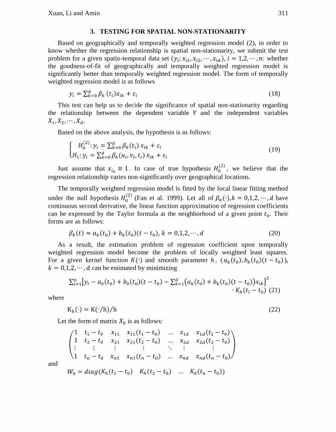
3. TESTING FOR SPATIAL NON-STATIONARITY
Based on geographically and temporally weighted regression model (2), in order to
know whether the regression relationship is spatial non-stationarity, we submit the test
problem for a given spatio-temporal data set ( ), : whether
the goodness-of-fit of geographically and temporally weighted regression model is
significantly better than temporally weighted regression model. The form of temporally
weighted regression model is as follows
∑ ( ) (18)
This test can help us to decide the significance of spatial non-stationarity regarding
the relationship between the dependent variable and the independent variables
.
Based on the above analysis, the hypothesis is as follows:
{ ( ) ∑ ( )
∑ ( )
(19)
Just assume that . In case of true hypothesis ( )
, we believe that the
regression relationship varies non-significantly over geographical locations.
The temporally weighted regression model is fitted by the local linear fitting method
under the null hypothesis ( )
(Fan et al. 1999). Let all of ( ), have
continuous second derivative, the linear function approximation of regression coefficients
can be expressed by the Taylor formula at the neighborhood of a given point . Their
forms are as follows:
( ) ( ) ( )( ), (20)
As a result, the estimation problem of regression coefficient upon temporally
weighted regression model become the problem of locally weighted least squares.
For a given kernel function ( ) and smooth parameter , ( ( ) ( )( ) ),
can be estimated by minimizing
∑ [ ( ) ( )( ) ∑ ( ( ) ( )( )) ]
( ) (21)
where
( ) ( ⁄ ) ⁄ (22)
Let the form of matrix is as follows:
(
( ) ( )
( ) ( )
( )
( )
,
and
( ( ) ( ) ( ))
Statistical Inference of Geographically and Temporally Weighted… 312
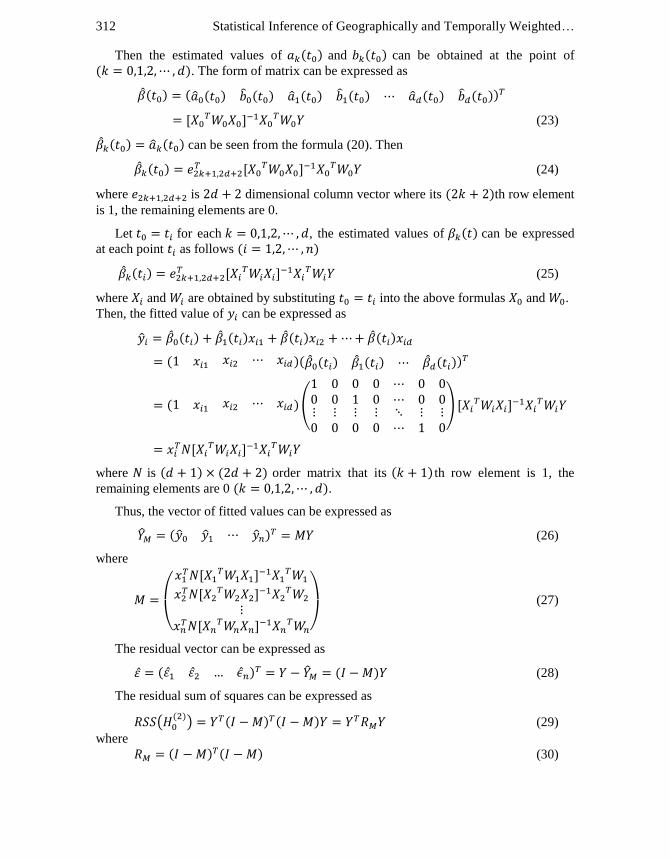
Then the estimated values of ( ) and ( ) can be obtained at the point of
( ). The form of matrix can be expressed as
( ) ( ( ) ( ) ( ) ( ) ( ) ( ))
[ ]
(23)
( ) ( ) can be seen from the formula (20). Then
( ) [
]
(24)
where is dimensional column vector where its ( )th row element
is 1, the remaining elements are 0.
Let for each , the estimated values of ( ) can be expressed
at each point as follows ( )
( ) [
]
(25)
where and are obtained by substituting into the above formulas and .
Then, the fitted value of can be expressed as
( ) ( ) ( ) ( )
( )( ( ) ( ) ( ))
( )(
) [ ]
[
]
where is ( ) ( ) order matrix that its ( ) th row element is 1, the
remaining elements are 0 ( ).
Thus, the vector of fitted values can be expressed as
( ) (26)
where
(
[
]
[
]
[
]
)
(27)
The residual vector can be expressed as
( ) ( ) (28)
The residual sum of squares can be expressed as
( ( )) ( ) ( ) (29)
where
( ) ( ) (30)
Xuan, Li and Amin 313
The vector of fitted values and the residual sum of squares for geographically and
temporally weighted regression model under the alternative hypothesis can be
expressed as (12) and (14).
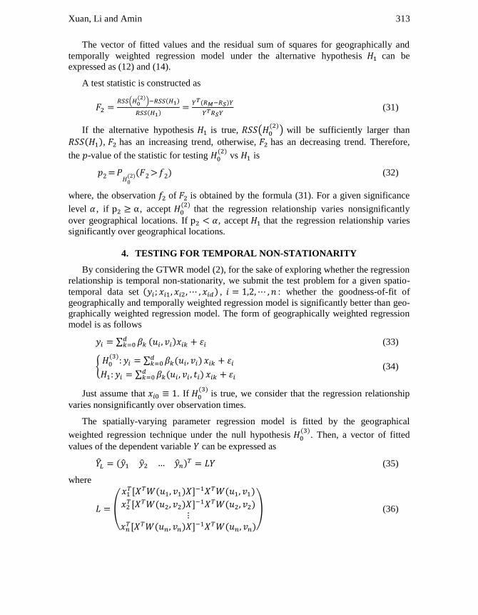
A test statistic is constructed as
(
( )) ( )
( ) ( )
(31)
If the alternative hypothesis is true, ( ( )) will be sufficiently larger than
( ), has an increasing trend, otherwise, has an decreasing trend. Therefore,
the -value of the statistic for testing ( )
vs is
( )( ) (32)
where, the observation of is obtained by the formula (31). For a given significance
level , if , accept ( )
that the regression relationship varies nonsignificantly
over geographical locations. If , accept that the regression relationship varies
significantly over geographical locations.
4. TESTING FOR TEMPORAL NON-STATIONARITY
By considering the GTWR model (2), for the sake of exploring whether the regression
relationship is temporal non-stationarity, we submit the test problem for a given spatio-
temporal data set ( ) , : whether the goodness-of-fit of
geographically and temporally weighted regression model is significantly better than geo-
graphically weighted regression model. The form of geographically weighted regression
model is as follows
∑ ( ) (33)
{ ( ) ∑ ( )
∑ ( )
(34)
Just assume that . If ( )
is true, we consider that the regression relationship
varies nonsignificantly over observation times.
The spatially-varying parameter regression model is fitted by the geographical
weighted regression technique under the null hypothesis ( )
. Then, a vector of fitted
values of the dependent variable can be expressed as
( ) (35)
where
(
[ ( ) ]
( )
[ ( ) ]
( )
[ ( ) ]
( ))
(36)
Statistical Inference of Geographically and Temporally Weighted… 314
( ) ( ( ), ( ), , ( ))
where ( ) ( ) , ( ) is any given point in the study area,
are the distance between ( ) and ( ) . Let ( ) ( ) , then we get the weighting matrix ( ) with kernal function
and bandwidth .
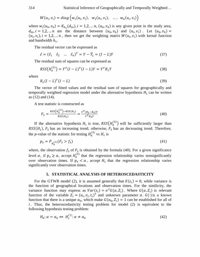
The residual vector can be expressed as
( ) ( ) (37)
The residual sum of squares can be expressed as
( ( )) ( ) ( ) (38)
where
( ) ( ) (39)
The vector of fitted values and the residual sum of squares for geographically and
temporally weighted regression model under the alternative hypothesis can be written
as (12) and (14).
A test statistic is constructed as
(
( )) ( )
( ) ( )
(40)
If the alternative hypothesis is true, ( ( )) will be sufficiently larger than
( ), has an increasing trend, otherwise, has an decreasing trend. Therefore,
the -value of the statistic for testing ( )
vs is
( )( ) (41)
where, the observation of is obtained by the formula (40). For a given significance
level , if , accept ( )
that the regression relationship varies nonsignificantly
over observation times. If , accept that the regression relationship varies
significantly over observation times.
5. STATISTICAL ANALYSIS OF HETEROSCEDASTICITY
For the GTWR model (2), it is assumed generally that ( ) , while variance is
the function of geographical locations and observation times. For the similicity, the
variance function may express as ( ) ( ) . Where ( ) is relevant
function of the variable ( ) and unknown parameter . ( ) is a known
function that there is a unique , which make ( ) can be established for all of
. Thus, the heteroscedasticity testing problem for model (2) is equivalent to the
following hypothesis testing problem:
( ) (42)
Xuan, Li and Amin 315
The model (2) is provided with heteroscedasticity under the alternative hypothesis ,
( ( )) . The penalized log-likelihood function of model (2) can be
expressed as (Sliverman et al. 1993)
( )
∑ ( ) ∑
( )
∑ ( ) ( )
(43)
where ( ) ( ( ) ( ) ( )) , is a diagonal matrix,
which is related to observed point ( ).
Let ( ( ) ), and is the estimated value of the parameter in model (2)
under the null hypothesis . By fitting the model (2) under the null hypothesis , the
estimated value of the parameter can be obtained. Then the residual at point is
defined as
∑ ( ) (44)
Just assume that , The estimated value of is denoted as follows
∑
(45)
For the heteroscedasticity testing problem of the model (2), the construction method
of test statistic is summarized into the following lemma:
Lemma 1:
If ( ( )
( )
( )
)
, ( ⁄ ) ,
( ⁄
⁄ ⁄ )
, where is order identity matrix,
( ) . Then, the SCORE test statistic of the problem (42) can be
expressed as
( ) (46)
Proof:
For the penalized log-likelihood function ( ) such as formula (43), the partial
derivatives on the parameter , ( ) and can be expressed as follows
( )
∑
( )
( )
∑
( )
( )
∑
( )
( )
[
( ) ]
( )
( ) ∑
( )
( )
∑ ( )
( )
∑
( )
( )
∑ ,*
( ) +
*
( )
( )
+
( )
( )
( )
-
Statistical Inference of Geographically and Temporally Weighted… 316
( )
∑
( )
( )
( )
∑
( )
( )
( )
∑
( )
( )
( ) ∑
( )
( )
( )
( ) ∑
( )
( )
( ) ( ) ∑
( ) ∑
( )
( )
( )
( )
Let is Fisher information array about the parameter , and is block matrix
corresponding to . At present, the estimated value of parameter be under the null
hypothesis , and ( ) . Thus
( )
( ) (47)
The form of Fisher information array can be expressed as
( ) (
+
where, is corresponding to parameter . is corresponding to parameter ( ), and
is corresponding to parameter , the elements are computed at . It is noted
that ( ) ( )
. Thus
* ( )
+
* ( )
( )+
* ( )
+
* ( )
( ) +
* ( )
( ) ( )+
* ( )
( ) +
Xuan, Li and Amin 317
* ( )
+
* ( )
( )+
* ( )
+
can be obtained by inverse matrix algorithm in block matrix. We have
[ ( ) (
*
( *]
[ ( ) (
*
( *]
[ ( ) (
*]
[ ]
*
+
*
( ⁄ ) ( ⁄ ) +
( )
For hypothesis testing problem (42), the SCORE test statistic (Eubank. 1988) can be
expressed as
[( ( )
)
( ( )
)]
( ) ( )
( )
* (
) ( ) (
) +
( )
Thus, the formula (46) is established.
If the alternative hypothesis is true, the test statistic has an increasing trend,
otherwise, has an decreasing trend. Therefore, the -value of the statistic for testing
vs is
( ) (48)
where, the observation of is obtained by the formula (46). For a given significance
level , if , accept ; otherwise, do not accept .
For simplicity, if the variance structure of is only related with one of in the
model (2), let
Statistical Inference of Geographically and Temporally Weighted… 318
( ) ( ) (49)
and ( )
. At present, we should pay attention to is a numerical value but
not a matrix. We have
( )
( )
(50)
Then
( )
(
⁄
⁄
⁄
,
(
,
∑ ( ⁄ )
and
(
,
(
)
(
,
∑ (∑
) ⁄
Thus, the SCORE test statistic can be expressed as
( )
[∑ (
⁄ ) ]
[∑ (∑
) ⁄
] (51)
6. COMPUTATION OF -VALUE
In the case of the previous fitting methods, even if the error terms in the
model are assumed to be independent and identically distributed as normal distribution
( ), in (16) is generally not distributed as an -distribution because is not
idempotent and the numerator and denominator are not independent. However, under the
assumption that the fitted value of the dependent variable is unbiased estimate of
( ), that is, ( ) ( ). can be expressed as a ratio of quadratic forms in error
terms so that we can use some distributional results of quadratic forms of normal variates
to compute the -value if we further assume that the error terms are normally distributed.
For this purpose, the following lemma is given:
Lemma 1:
Under the assumption that the fitted value of the dependent variable is the unbiased
estimate of ( ), can be expressed as
Xuan, Li and Amin 319
(
( )) ( )
( ) ( )
(52)
where ( ) is the error vector of the model.
Proof:
under the null hypothesis ( )
, a linear regression model is valid to the data, and it is
well known that
( ( )) (53)
On the other hand, under the assumption of ( ) ( ), we have
( ) ( ) ( )
[ ( )] ( ) (54)
Thus
( ) ( ) ( )
( ) ( )
(55)
The lemma is then proved by substituting (53) and (55) into (16).
Similarly, we can prove that and can be expressed as
( )
(56)
( )
(57)
This section provides distribution approximation method (Cleveland et al. 1988) to
compute the previous -values. The main idea of distribution approximation method is
to approximate normal variable quadratic distribution of the numerator and denominator
in the test statistic by distribution with appropriate multiples and degrees of freedom
respectively, then the distribution of test statistic is approximated by distribution with
appropriate degrees of freedom. Below, we discuss a brief introduction about approxima-
tion method for distribution.
Let , where ( ) and is order semi-positive definite real symmet-
ric matrix. If is idempotent matrix, is a random variable distributed as distribution
with degrees of freedom ( ). The distribution of is generally approximated by .
Through determining the constants and , make the expectation and variance of be
equal to the expectation and variance of .
( ) , (
) , and ( ) ( ), ( ) ( ).
Let
{ ( )
( )
Statistical Inference of Geographically and Temporally Weighted… 320
Then
( )
( )
[ ( )]
( ) (58)
For quadratic form of normal variate
, where ( ), and are semi-
positive definite real symmetric matrices. If and are idempotent, and ,
then is distributed as distribution with degrees of freedom ( ), and ( ). The
distribution of is generally approximated by for . Let
(
) ⁄
(
) ⁄
( )
( ) (59)
thus, we apply ( ) to approximate the distribution of .
Under the assumption that the fitted values of the dependent variable is the
unbiased estimate of ( ), we provide the approximate computing formula of -value
based on distribution approximation method.
For the test statistic , we have
( )( )
( ) (
( )
)
( ) (
( )
( )
( )
( )
( ) )
( ( ) ( )
( ) )
where [ ( )]
( ) ,
[ ( )]
( )
. ( ) is a random variable distributed as
distribution with degrees of freedom , .
Similarly, for the test statistics and , we have
( )( ) ( ( )
( )
( ) )
where [ ( )]
( ) ,
[ ( )]
( )
. ( ) is a random variable distributed as
distribution with degrees of freedom , .
( )( ) ( ( )
( )
( ) )
where [ ( )]
( ) ,
[ ( )]
( )
. ( ) is a random variable distributed as
distribution with degrees of freedom , .
Here, we provide the approximate formula to compute -value for the test statistic .
Let
√ (60)
Xuan, Li and Amin 321
that is
* ∑ (∑
)
⁄
+
(∑ ⁄
∑ )
* ( ) ( )
( ) ( ) +
where
( )
( ), [ ∑ (∑
) ⁄
]
If the estimation bias of regression function can be ignored, that is, ( ) .
Then, we have
* ( ) ( )
( ) ( ) +
(
)
where
( ) ( ) ( )
( )
Then
( )( )
( )( √ ) ( √ )
( )( √ √ )
( ) (
√
√
*
( ) (
( )
( )
√
( )
( )
( )
( )
√
*
( ( )
( )
√
( )
( )
( )
√
*
where [ ( )]
( )
, [ ( )]
( )
. ( ) is a random variable distributed as
distribution with and degrees of freedom.
7. TESTING FOR SPATIAL NON-STATIONARITY
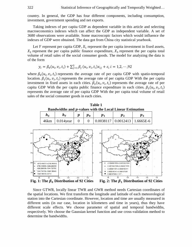
To examine the applicability of GTWR, a case study was implemented using per
capita GDP observed between 2004 and 2013 in Chinese 92 cities. The main purpose of
the analysis is to explore the underlying spatio-temporal patterns of per capita GDP in the
mainland of China and to analyze of the factors which affect per capita GDP.
GDP is often used as indicators of the development of economics. It can not only
reflect a country's economic performance, but also reflect the strength and wealth of a
Statistical Inference of Geographically and Temporally Weighted… 322
country. In general, the GDP has four different components, including consumption,
investment, government spending and net exports.
Taking indexes of per capita GDP as dependent variable in this article and selecting
macroeconomics indexes which can affect the GDP as independent variable. A set of
3680 observations were available. Some macroscopic factors which would influence the
indexes of GDP were obtained. The data got from China city statistical yearbook.
Let represent per capita GDP, represent the per capita investment in fixed assets,
represent the per capita public finance expenditure, represent the per capita total
volume of retail sales of the social consumer goods. The model for analyzing the data is
of the form
( ) ∑ ( )
where ( ) represents the average rate of per capita GDP with spatio-temporal
location. ( ) represents the average rate of per capita GDP With the per capita
investment in fixed assets in each cities. ( ) represents the average rate of per
capita GDP With the per capita public finance expenditure in each cities. ( ) represents the average rate of per capita GDP With the per capita total volume of retail
sales of the social consumer goods in each cities.
Table 1
Bandwidths and -values with the Local Linear Estimation
46km 0.014year 0 0 0.0038117 0.0012413 1.6665E-6
Fig. 1: The Distribution of 92 Cities Fig. 2: The Distribution of 92 Cities
Since GTWR, locally linear TWR and GWR method needs Cartesian coordinates of
the spatial locations. We first transform the longitude and latitude of each meteorological
station into the Cartesian coordinate. However, location and time are usually measured in
different units (in our case, location in kilometers and time in years), thus they have
different scale effects. We choose parameter of spatial and temporal bandwidths,
respectively. We choose the Gaussian kernel function and use cross-validation method to
determine the bandwidths.
Xuan, Li and Amin 323
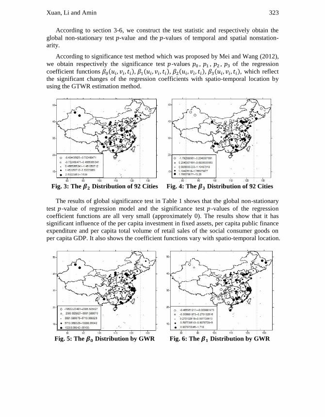
According to section 3-6, we construct the test statistic and respectively obtain the
global non-stationary test -value and the -values of temporal and spatial nonstation-
arity.
According to significance test method which was proposed by Mei and Wang (2012),
we obtain respectively the significance test -values , , , of the regression
coefficient functions ( ), ( ), ( ), ( ), which reflect
the significant changes of the regression coefficients with spatio-temporal location by
using the GTWR estimation method.
Fig. 3: The Distribution of 92 Cities Fig. 4: The Distribution of 92 Cities
The results of global significance test in Table 1 shows that the global non-stationary
test -value of regression model and the significance test -values of the regression
coefficient functions are all very small (approximately 0). The results show that it has
significant influence of the per capita investment in fixed assets, per capita public finance
expenditure and per capita total volume of retail sales of the social consumer goods on
per capita GDP. It also shows the coefficient functions vary with spatio-temporal location.
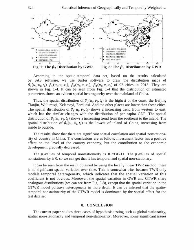
Fig. 5: The Distribution by GWR Fig. 6: The Distribution by GWR
Statistical Inference of Geographically and Temporally Weighted… 324
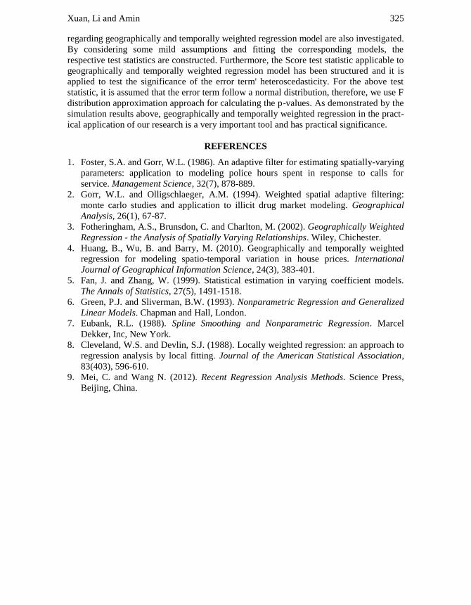
Fig. 7: The Distribution by GWR Fig. 8: The Distribution by GWR
According to the spatio-temporal data set, based on the results calculated
by SAS software, we use Surfer software to draw the distribution maps of
( ) ( ) ( ) ( ) of 92 cities in 2013. They are
shown in Fig. 1-4. It can be seen from Fig. 1-4 that the distribution of estimated
parameters shows an evident spatial heterogeneity over the mainland of China.
Thus, the spatial distribution of ( ) is the highest of the coast, the Beijing
Tianjin, Wulumuqi, Kelamayi, Eerduosi. And the other places are lower than these cities.
The spatial distribution of ( ) shows a increasing trend from western to east,
which has the similar changes with the distribution of per capita GDP. The spatial
distribution of ( ) shows a increasing trend from the southeast to the inland. The
spatial distribution of ( ) is the lowest of inland of China, increasing from
inside to outside.
The results show that there are significant spatial correlation and spatial nonstationa-
rity of country in China. The conclusions are as follow. Investment factor has a positive
effect on the level of the country economy, but the contribution to the economic
development gradually decreased.
The -values of temporal nonstationarity is 8.793E-11. The -values of spatial
nonstationarity is 0, so we can get that it has temporal and spatial non-stationary.
It can be seen from the result obtained by using the locally linear TWR method, there
is no significant spatial variation over time. This is somewhat trite, because TWR only
models temporal heterogeneity, which indicates that the spatial variation of this
coefficient is not obvious. Moreover, the spatial variation in GWR and GTWR share
analogous distributions (we can see from Fig. 5-8), except that the spatial variation in the
GTWR model portrays heterogeneity in more detail. It can be inferred that the spatio-
temporal nonstationarity of the GTWR model is dominated by the spatial effect for the
test data set.
8. CONCLUSION
The current paper studies three cases of hypothesis testing such as global stationarity,
spatial non-stationarity and temporal non-stationarity. Moreover, some significant issues
Xuan, Li and Amin 325
regarding geographically and temporally weighted regression model are also investigated.
By considering some mild assumptions and fitting the corresponding models, the
respective test statistics are constructed. Furthermore, the Score test statistic applicable to
geographically and temporally weighted regression model has been structured and it is
applied to test the significance of the error term' heteroscedasticity. For the above test
statistic, it is assumed that the error term follow a normal distribution, therefore, we use F
distribution approximation approach for calculating the p-values. As demonstrated by the
simulation results above, geographically and temporally weighted regression in the pract-
ical application of our research is a very important tool and has practical significance.
REFERENCES
1. Foster, S.A. and Gorr, W.L. (1986). An adaptive filter for estimating spatially-varying
parameters: application to modeling police hours spent in response to calls for
service. Management Science, 32(7), 878-889.
2. Gorr, W.L. and Olligschlaeger, A.M. (1994). Weighted spatial adaptive filtering:
monte carlo studies and application to illicit drug market modeling. Geographical
Analysis, 26(1), 67-87.
3. Fotheringham, A.S., Brunsdon, C. and Charlton, M. (2002). Geographically Weighted
Regression - the Analysis of Spatially Varying Relationships. Wiley, Chichester.
4. Huang, B., Wu, B. and Barry, M. (2010). Geographically and temporally weighted
regression for modeling spatio-temporal variation in house prices. International
Journal of Geographical Information Science, 24(3), 383-401.
5. Fan, J. and Zhang, W. (1999). Statistical estimation in varying coefficient models.
The Annals of Statistics, 27(5), 1491-1518.
6. Green, P.J. and Sliverman, B.W. (1993). Nonparametric Regression and Generalized
Linear Models. Chapman and Hall, London.
7. Eubank, R.L. (1988). Spline Smoothing and Nonparametric Regression. Marcel
Dekker, Inc, New York.
8. Cleveland, W.S. and Devlin, S.J. (1988). Locally weighted regression: an approach to
regression analysis by local fitting. Journal of the American Statistical Association,
83(403), 596-610.
9. Mei, C. and Wang N. (2012). Recent Regression Analysis Methods. Science Press,
Beijing, China.


