Embed Size (px)
Citation preview

STATISTICS IN TRANSITION new series, Spring 2015
1
STATISTICS IN TRANSITION new series, Spring 2015
Vol. 16, No. 1, pp. 1–26
STOCHASTIC GOALS IN FINANCIAL PLANNING FOR
A TWO-PERSON HOUSEHOLD
Radosław Pietrzyk1, Paweł Rokita
2
ABSTRACT
In household financial planning two types of risk are typically being taken into
account. These are life-length risk and risk connected with financing. In addition,
also various types of events of insurance character, like health deterioration, are
sometimes taken into account. There are, however, no models addressing
stochastic nature of household financial goals. The last should not be confused
with modelling factors that influence performance of financing the goals, which is
a popular research topic. The problem of modelling goals themselves is, in turn,
not so well explored. There are two main characteristics that describe a goal:
magnitude and time. At least for some goals one or both of these characteristics
may show a stochastic nature. This article puts forward a proposition of working
goal time and magnitude into a household financial plan and taking their
distributions into account when optimizing the plan. A model of two-person
household is used. The decision variables of the optimization task are
consumption-investment proportion and division of household investments
between household members.
Key words: financial goals, personal finance, intertemporal choice, financial plan
optimization, stochastic goals.
1. Introduction
The aim of this article is to present a concept of a household financial plan optimization model that allows for stochastic character of household goals, in respect of goal realization time and magnitude.
The model assumes that the household maximizes its value function, which is composed of expected discounted utilities of consumption and bequest.
For the financial plan optimization procedure, the value function plays the role of a goal function. This article, however, is not meant to propose an optimization technique. It is rather intended to discuss a concept of how to formulate the problem. Optimization of a financial plan with a number of 1 Wroclaw University of Economics. E-mail: [email protected]. 2 Wroclaw University of Economics. E-mail: [email protected].

2 R. Pietrzyk, P. Rokita: Stochastic goals in financial …
dynamic stochastic factors is described from operational research perspective by Konicz, et al. (2014), for instance. The last builds on the results by Gayer et al. (2009) and Richard (1975). Also, a multi-person household case was analyzed (Bruhn and Steffensen, 2014). A comprehensive introduction to stochastic programming in finance may be found in the positions by Ziemba (2003) and Vickson and Ziemba (2006). A more general summary of the concept and methods of stochastic programming models is presented by Ruszczyński and Shapiro (2003).
As it has already been mentioned, the main focus is to take account of uncertainty about goal realization, but not in the sense of the question if the household is able to afford them, but rather in the sense of stochastic nature of such goal characteristics as time and magnitude of the need (in financial terms) the goal is expected to satisfy. The subject-matter of this article does not cover the risk of financing. For example, if an investment is meant as a future source of financing for the goal, the market risk of assets used as part of the investment is not in the scope of interest here. Also, if a credit is planned for the realization of the goal, the interest rate risk connected with the credit is not the issue to be discussed in this article.
The model belongs to the area of life-cycle financial planning in personal finance. It uses the basic concepts present in this field of research. In the literature on life-long financial planning a lot of research has been done in the areas of consumption optimization and dynamic portfolio optimization. The first current builds on Modigliani, Brumberg (1954), Ando, Modigliani (1957) and Yaari (1965), whereas the dynamic asset allocation research – on the works by Merton (1969, 1971) and Richard (1975). Further research in life cycle planning with dynamic stochastic properties of asset prices was done by Cox and Huang (1989). An important issue in personal finance is also a trade-off between life insurance and capital-based protection against unexpected events in the area of survival process (Ibbotson et al. 2005, Huang et al., 2008). Also, the problem of two-person household was tackled by personal finance researchers. Kotlikoff and Spivak (1981) investigated the influence of longevity risk sharing between household members (a married couple) on the demand for annuities. Hurd (1999) constructed a two-person generalization of the classical (Yaari 1965) life-cycle model and presented an analytical solution to the consumption optimization problem for a couple. Brown and Poterba (2000) analysed advantages of joint annuities suited to the needs of married couples, with reference to the longevity-risk-sharing effect discussed earlier by Kotlikoff and Spivak (1981). Generally speaking, the current state of the art covers many important aspects of consumption transfer in life-cycle financial planning in the sense by Bodie et al. (2008), that is – in the two directions: between periods (by means of saving and investments) and between optimistic and pessimistic scenarios (by means of insurance, but also risk sharing). The last (considering scenarios) is a way of addressing a more general problem, namely – uncertainty. In this area, the following stochastic factors influencing the financial plan were taken into

STATISTICS IN TRANSITION new series, Spring 2015
3
account: rates of return on investment, length of life (also in a bivariate case), health condition, labour income, and sometimes also damage to physical property. What remains a rather unexplored field is the way financial goals themselves may behave.
It is much more popular to take into consideration the risk of having insufficient means to finance a goal on a specified date (it refers to pre-financing and post-financing) than the risk that, for instance, the time when the household really needs to accomplish this goal will be shifted in time. This article presents a proposition that may serve as a starting point for filling in this gap. For example, an important risk factor influencing the performance of the household financial plan is the time of a child's birth. This may of course differ from a planned or desired time. There is, however, no research on statistical properties of this source of uncertainty in the literature. And, consistently, in personal finance, it does not belong to the set of risk factors that are modelled using statistical methods as part of financial planning. Starting a discussion about conditional distribution of a child's birth, under the condition of planned time, seems a natural step further in the development of personal finance research area.
It seems necessary to explain that the proposition put forward in this article provides a general framework within which more detailed models may be developed. For instance, assumed interdependencies between household financial goals may be in fact different in details, but the provided example is sufficient to outline the general idea. Moreover, for some stochastic elements of the model, only putative properties are discussed, without even suggesting types, nor even general families, of parametric distributions that might be used.
The paper is organized in the following way. Section 2 shortly sums up the basic version of the model, upon which the current concept is developed. Types of financial goals are discussed in section 3. In this section also some definitions and assumptions are presented. Sections 4 and 5 are devoted to the main subject of this article, namely – stochastic character of the goals and interdependencies between them (section 4) and the way these properties may be reflected in value function of the household (section 5). The last section contains conclusions.
2. An outline of the model
The model developed here is based on its basic version presented by Feldman, Pietrzyk and Rokita (2014a, 2014c) and Pietrzyk and Rokita (2014). This is a discrete time, two-person household, life-long financial plan model. In the basic version it assumed only two financial goals: retirement and bequest. Consumption is optimized in the life cycle of the household, both in accumulation phase and in retirement.
The dates of death of the two persons are the only risk factors in the basic version of the model. Plans differ in respect of risk. Some are very immune against even very large deviations of dates of death from their expected values,

4 R. Pietrzyk, P. Rokita: Stochastic goals in financial …
some other are very sensitive. They are exposed to premature-death risk and longevity risk. In the two-person case, premature-death risks play not less important role than longevity (and this statement remains valid even if the household has no bequest motive).
The only two goals of the basic model are set in different ways. Whereas retirement is set explicitly as a goal to be accomplished, in terms of time and magnitude, the bequest motive is merely declared, only in order to pass the information to the value function of the household if utility of residual wealth is to be calculated or not.
It is assumed that the retirement capital accumulated until retirement date of a given person is fully spent on a life annuity assigned to this person. The household has, yet, a choice whether to invest in building retirement capital of the first, the second or both persons in any proportions.
One of the main features of a two-person household, as compared to a single-individual case, is life-time risk sharing. It allows for building plans with the so-called “partial retirements” – compare Full-Partial, Partial-Full and 2×Partial
retirement as defined by Feldman, Pietrzyk and Rokita (2014a). The possibility of investing in less than 2×Full retirement in the sense by Feldman et al. (2014a) broadens the spectrum of possible proportions between consumption and investments the household may choose.
A deterministic growth pattern of consumption, which is usually a constant growth rate in real terms, is assumed. This constitutes the basic path of
consumption. Upon this, some additional consumption may be put on. In extended versions of the model, going beyond the two-goal framework, it is usually the result of the realization of some goals (like, for instance, new consumption structure connected with a child in the household).
It is also assumed that at the starting time of the plan the household invests the whole part of income which is not consumed (there is no surplus generated). Since the basic version of the model does not assume any other financial goals than retirement, the investment is here understood as investing for retirement. In subsequent periods, because of differences in income and consumption growth rates, there may be some additional unconsumed and uninvested surplus. Saying that the surplus is not invested is a mental shortcut. More precisely – one cannot assume in advance that the surplus will be invested at a high rate (unplanned investments that, in addition, need to be very liquid, because they are used to cover some intermittent shortfalls).
The surplus cumulated until a moment may be used to smoothen consumption path in the next periods. But it must be pointed out that if there is a goal of creating a safety cash reserve to play a similar role (not discussed in this work as a separate type of goal), then this is not treated as a part of a cumulated surplus. It may be created from the surplus, but if it is done on purpose, the reserve disappears from the account of the surplus. Creating it should be treated as goal realization.
STATISTICS IN TRANSITION new series, Spring 2015
5
The plan is optimized by maximization of the value function of the household, given by equation (2) in section 5. The decision variables are:
• consumption-investment proportion (given by consumption rate in the first period),
• division of investment between persons (given by first-period proportion of Person 1 investment).
All parameters of the model like incomes, returns on investments, growth rates, macroeconomic parameters, etc., are assumed to be revised on a regular basis (at least once a year as recommended). Each plan revision session includes new optimization. This allows avoiding the need of making long-term forecasts. All parameters are assumed to be valid for the whole planning period, but they are updated every year. Plan revisions include also corrections in goal time and magnitude. No modifications of goal structure are made automatically as a result of optimization. They may be introduced only by the decision of the household. The only variables that are changed in the optimization procedure are the two aforementioned decision variables.
As it has already been mentioned, any changes in time or size of the goals due to lack of financing, too risky financing, or any other reasons that are not intrinsic to the goals themselves, are not the subject of the analysis in this work.
3. Financial goals
Besides securing some acceptable life standard for all household members throughout the whole life of the household, households tend to realize yet some ambitions and dreams that, if given some planning rigor to, may be called life objectives. Some of these objectives may be expressed in financial terms and included into a quantitative model as financial goals. The aim of a financial plan is maximization of the value function of the household and fulfilling at the same time all constraints, including accomplishment of financial goals. In this article an attempt is made to take into account a stochastic character of time and magnitude with which the goals are realized. Defining the terms “financial goal” and “realization of financial goal” first seems necessary to avoid confusion. It has also to be specified which financial goals will be considered in the discussion, and finally, which of them are to be formally included into the model.
3.1. Definitions and assumptions
According to the definition of the household by Zalega (2007), a household is an autonomous economic entity distinguished according to the criterion of
individual property, making decisions about consumption on the basis of its
preferences and existing constraints.
Here, in this paper a two-person household is considered. It is understood as a household with two decision makers, called also main members, who (at least as

6 R. Pietrzyk, P. Rokita: Stochastic goals in financial …
far as their predetermination at the moment of plan preparation is concerned) intend to remain members of the household until its end. This does not really exclude cases with more or less members (comp. Feldman, Pietrzyk and Rokita, 2014a, 2014c; Pietrzyk and Rokita, 2014) if one or two main household members are distinguished.
It is assumed that households maximize utility of consumption throughout their whole life cycle. The household has also some life objectives that its members want to accomplish in certain time and to a certain extent. These objectives are kinds of constraints for the consumption utility maximization. But the true time and cost of realization of the objectives is not certain indeed. Here, the focus is on the uncertainty inherent in the objectives themselves, not in the tools of their realization like financing.
From the point of view of the model discussed here the life objectives may be divided into two groups: financial and non-financial. The model is intended to include in a household life-long financial plan those that are of financial nature. They will be further called financial goals (comp. Definition 1).
Definition 1. Financial goal
To provide financial means for covering a negative cash flow or a series of negative cash flows of a substantial value, prearranged as to time and magnitude and isolated from the basic path of consumption (comp. explanation of the term “basic path of consumption” in section 2).
Satisfaction resulting from realization of the financial goals is here identified with the utility of consumption. The financial goals may, of course, give also other kinds of satisfaction to the household, but this is not taken into account in the model.
The most important financial goals may include, for example: purchase of a house, leaving a bequest, covering costs of bringing up children and covering costs of their education.
Even though the main goal of the household is to guarantee a satisfactory life standard to all household members throughout the whole life cycle, vast part of which is realized by means of preserving a desired level of the basic path of consumption. This is why the goal is not distinguished as one of financial goals.
As to the non-financial objectives, they influence decisions of the households in many respects, including financial decisions, but they themselves are not expressed in financial terms. These objectives may cover, for instance, finding a suitable partner, or just broadly understood self-fulfilment in personal and professional area. The realization of non-financial objectives may indirectly modify cash flows of the household, because it may change propensity to consume, motivation to save and invest, etc.
As it has already been mentioned, only financial goals are considered in the model. The model is intended to allow for stochastic character of goal realization in two respects: time and magnitude. Goal realization is understood here as specified by the Definition 2:

STATISTICS IN TRANSITION new series, Spring 2015
7
Definition 2. Goal realization
A negative cash flow or series of negative cash flows connected with a financial goal.
It is important to avoid confusion between the three related terms: (a) life objective, (b) financial goal of providing required financial means at a given time, (c) goal realization.
A practical difference between these terms may be easily explained by the example of having-a-child objective. Is the time of a child's birth a stimulant, destimulant or nominant in the sense of its influence on the value function of the household? Of course, the time at which the household is (in financial sense) ready to bring up children – comp. (b) financial goal – is a destimulant (the earlier the better). But the time when the child is born and the period of higher consumption starts – comp. (c) goal realization – is a nominant (the closer to the planned time the better). And finally, whether the time of birth is a stimulant, destimulant or nominant from a general life situation perspective (a) is really hard to say and this piece of work does not even attempt to answer this question.
Five types of goals are distinguished in the model. They are treated in different manners. There is a set of characteristics according to which the goals may be grouped. They are: time of realization, goal magnitude in monetary terms, number of cash flows needed to realize the goal. Another important feature is the role of the financial goal in the household wealth. Realization of some goals contributes to the household wealth (like buying a house), whereas other are by their nature more similar to consumption (put differently, their realization is just consumption, but isolated from its basic path).
The distinguished types are: • Type I – Child(ren), • Type II – Retirement, • Type III – House (residential real estate bought in order to live there, not as
kind of investment), • Type IV – Endowment, • Type V – Bequest.
It is important to emphasize that in this model any investments are treated as tools supporting financing realization of some goals of the household. Investments and goals are two separated categories. Making an investment cannot be a goal. Nevertheless, there is a strong link between the first and the second. Namely, if there are any investments in the model, they are assigned to some corresponding goals. This is, however, not a bijective relation. Two or more investments may be used to support financing of one goal, and also one investment may be used to provide financing of two or more goals (Feldman, Pietrzyk, Rokita, 2014b). Reservations are expressed about the fact that if a purchase of an asset (financial or non-financial) is treated as an investment, then

8 R. Pietrzyk, P. Rokita: Stochastic goals in financial …
this purchase is not a goal itself. It is rather used to finance some goals. The inverse does not hold, because realizing some types of goals like buying a house for own residential needs, may contribute to the total wealth of the household and then be used to finance some other goals (bequest, for example). In more details the issue is explained in the subsection 30.
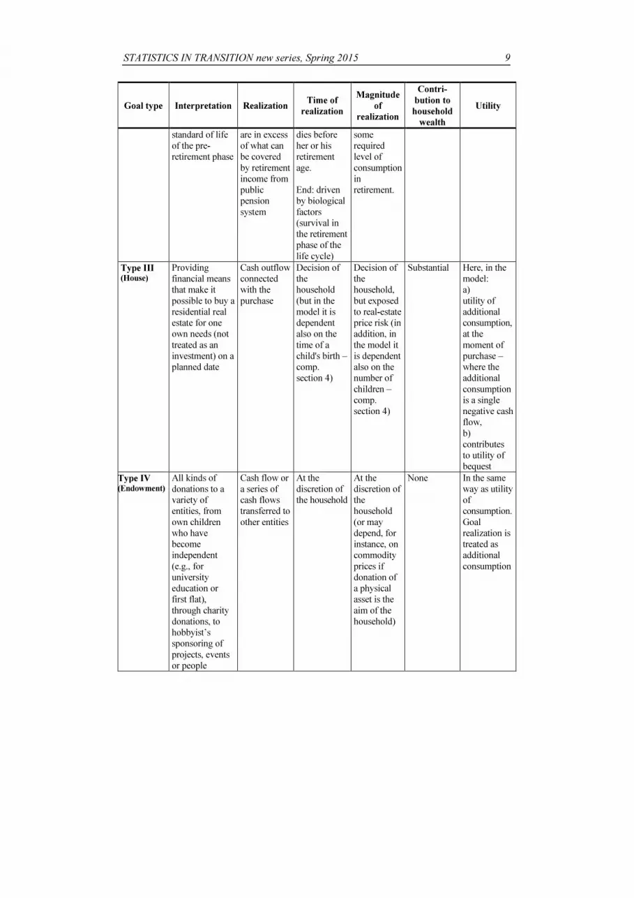
3.2. Goal comparison
The five types of goals are described below in terms of the following criteria: • Interpretation – general practical interpretation of the goal, • Realization – how goal realization is expressed, • Time and Magnitude of realization – determinants of the main characteristics,
namely – time and magnitude (whether they are random or deterministic, if the household controls them or they are out of control by the household, whether they depend on some other factors and if the dependence is of stochastic or deterministic nature),
• Contribution to household wealth – if the goal realization contributes to household wealth or is just a particular kind of consumption (isolated from the basic path of consumption but not different in its nature from consumption),
• Utility – when and for how long (periods/cash flows) utility of goal realization is measured.
The comparison of goal types is presented in the Table 1.
Table 1. Goal types and their characteristics
Goal type Interpretation Realization Time of
realization
Magnitude
of
realization
Contri-
bution to
household
wealth
Utility
Type I (Child)
Being able to provide for additional consumption needs throughout the period when the child is a household member (usu. from birth to becoming independent)
Additional consumption. May be expressed as a percentage or absolute increase in consumption, prevailing throughout the period when the child remains in the household
Main characteristic. Stochastic, but the household declares some planned time
(To a vast extent) a derivative of general standard of life assumed by the household
None Prolonged. Utility of consumption in many periods.
Type II (Retirement)
Providing financial means for maintaining in the retirement period the
A series of consumption expenditures in retirement period that
Start: legally determined (retirement age) unless the person
At the discretion of the household, declaring
None Prolonged. Utility of consumption in many periods.
STATISTICS IN TRANSITION new series, Spring 2015
9
Goal type Interpretation Realization Time of
realization
Magnitude
of
realization
Contri-
bution to
household
wealth
Utility
standard of life of the pre-retirement phase
are in excess of what can be covered by retirement income from public pension system
dies before her or his retirement age. End: driven by biological factors (survival in the retirement phase of the life cycle)
some required level of consumption in retirement.
Type III (House)
Providing financial means that make it possible to buy a residential real estate for one own needs (not treated as an investment) on a planned date
Cash outflow connected with the purchase
Decision of the household (but in the model it is dependent also on the time of a child's birth – comp. section 4)
Decision of the household, but exposed to real-estate price risk (in addition, in the model it is dependent also on the number of children – comp. section 4)
Substantial Here, in the model: a) utility of additional consumption, at the moment of purchase – where the additional consumption is a single negative cash flow, b) contributes to utility of bequest
Type IV (Endowment)
All kinds of donations to a variety of entities, from own children who have become independent (e.g., for university education or first flat), through charity donations, to hobbyist’s sponsoring of projects, events or people
Cash flow or a series of cash flows transferred to other entities
At the discretion of the household
At the discretion of the household (or may depend, for instance, on commodity prices if donation of a physical asset is the aim of the household)
None In the same way as utility of consumption. Goal realization is treated as additional consumption

10 R. Pietrzyk, P. Rokita: Stochastic goals in financial …
Goal type Interpretation Realization Time of
realization
Magnitude
of
realization
Contri-
bution to
household
wealth
Utility
Type V
(Bequest)
Treated in a different way than other types. Interpreted as wealth at the moment of household end. This includes cumulated surplus and other assets. Particular role in the bequest mass is played by a house or flat bought as realization of type III goal.
Treated in a different way than other types. The bequest is just the wealth of the household passed to the descendants.
Not defined in terms of required magnitude and planned time. Instead, the household declares just bequest motive and chooses the value of its parameter (comp. section 5, subsection 0) Time of realization is determined by conditions of biological nature, which is the time of death of both household members. Magnitude of type V goal depends in the model on the household decision, but in a different way than it is for other goals. The declared bequest motive parameter just passes to the value function of the household the information on how important utility of bequest is to the household members.
The bequest is the residual wealth of the household
Utility of bequest (separate function)
3.3. Special cases – goals contributing to household wealth and resulting
utility issues
As it has already been mentioned (comp. subsection 0), the realization of a goal may have the effect of becoming a kind of investment. This is when goal realization consists in buying an asset that is of a durable nature.
This situation is encountered in the case of the Type II goal, that is – a house. One of the most important characteristics of this goal is that it contributes to household wealth. The real estate remains a part of household fixed assets for a long period (often until the household end). If the house or flat is sold earlier and a new one is bought instead, the new purchase may be treated as a next phase of realization of the same goal or the next goal. There is, yet, a technical question that needs to be answered before accepting such interpretation. As it has already been explained, utility in the model is only utility of consumption and utility of bequest. Utility of consumption attached to the goals is understood as utility of goal realization, where goal realization is a negative cash flow. This is logically consistent because the negative cash flows for goal realization and basic path of

STATISTICS IN TRANSITION new series, Spring 2015
11
consumption (also a series of negative cash flows) are identical in their nature (albeit magnitudes and regularity may differ). In the case of goals that do not contribute to household wealth, no further explanation to that is needed. But if realization of the goal is connected with a purchase of some component of fixed assets, treating it just as consumption is controversial. It is treated in this way in the model, but to avoid a have-one's-cake-and-eat-it-too paradox a concept of negative consumption is introduced, as described by Definition 3.
Definition 3. Negative consumption (also: inverted consumption,
deconsumption)
If a component of fixed assets of the household is purchased as part of goal realization (and thus the cash outflow connected with the purchase enters utility of consumption), then the cash inflow from selling this component at some later time is also taken into account in the utility of consumption as consumption with negative sign, and is called negative consumption (or inverted consumption or deconsumption).
Changing a flat or house into a new one is, thus, treated as a negative consumption equal (as far as absolute values are concerned) to the price obtained for the old house and positive consumption equal to the price paid for the new one. Effectively, utility of net sum of negative and positive consumption is taken. In this way, utility is measured only for the part of the new house value that is in excess over the old house value.
4. Stochastic nature of goals and their interdependencies
To show the way in which the goals may be taken into account in the value function of the household, it is not necessary to identify the distributions precisely. Knowledge of some of their general properties may be, however, useful. Of course, to construct a fully functional model, the detailed probabilities will be needed. The next important question is about the dependence between the goals. Constructing a model with a multivariate distribution of times and magnitudes for all goals would be a very tough task. And such approach would make the model hardly applicable in practice. In the proposition put forward here the relationships between some chosen goals are simplified to deterministic influence.
4.1. Goal dependency map
First, a map of relationships between the goals was created. It is a proposition only, but based on life experience, logical reasoning and general common knowledge of the nature of the goals. It is, yet, a simplification and it should be treated as such. The simplification is justified by the fact that the plan is revised every year (comp. section 2) and the goals may be shifted in time, added, removed or modified in respect of magnitude by the household. Thus, the attempt

12 R. Pietrzyk, P. Rokita: Stochastic goals in financial …
to include all possible stochastic and deterministic relationships might give only a spurious impression of precision. What is more important here is constructing a model of general influence structure. As a result, a kind of causal network of influences, mainly of deterministic character, was obtained. It is to a vast extent of (a kind of) hierarchical structure, because the direction of influences in this model is such that some goals rather exert influence, whereas other ones are rather influenced. The map of relationships between goals is constructed on the basis of the assumption that the main event in life of a household is birth of the first child. Thus, it may be said that it is the most “influential” one in the aforementioned hierarchy of influences.
A general map of relationships between goals for a stylized typical household may look for example like the one in the Figure 1. Arrows indicate influence directions.
Figure 1. Stylized map of relationships between goals
In Figure 1 the following influences are marked: • Time of house purchase is influenced by the time of a child's birth, and
magnitude of this goal is influenced by the number of children (in further discussion the second relation is neglected).
• Time of endowment may be influenced by the time when children appear (particularly if it is the first flat for a child, study for children or some kind of dowry). Magnitude of endowment depends on the number of children if the addressee of the endowment are children of the main household members.
• Magnitude of bequest is not directly controlled by the household, but it depends on the bequest motive parameter, which is at the discretion of household members. The bequest motive may, in turn, depend on the number of children. Also, the value of the house contributes to bequest, since the house is a part of wealth that may be bequeathed. Thus, the goal “house” and the goal “child” influence the magnitude of bequest.

STATISTICS IN TRANSITION new series, Spring 2015
13
• Retirement income may be (partially) obtained from inverted mortgage secured by the house the person lives in. Thus, the size of retirement is influenced by the value of the house.
The model of the goal relationship map may be used to construct a “child-driven” model of the household life-long financial plan. Certainly, if the household does not plan children, all dependencies between the time of a child's birth and other goals disappear. For example, Type III goal (House) is then not influenced by any goal in this model, but may still exert influence on other goals.
If the household plans a child (children), stochastic time of a child's birth (conditional on the planned time) is added to the main sources of uncertainty from the basic version of the model (lifetimes of the two main household members). For the sake of simplicity it may be assumed that the dates of buying a house and making an endowment are just shifted by a constant number of years in relation to the date of the first child's birth (let the shifts be denoted by Δ
handΔ
e,
respectively).
4.2. Time and magnitude distributions
It is proposed to distinguish four distributions:
• for the time of realization of the type I goal (Child) – conditional distribution of a child's birth, under the condition of the planned time,
• for magnitude of the type III goal (House) – distribution of real estate price at the moment of purchase,
• for magnitude of the type IV goal (Endowment) – none or distribution of (commodity/real estate) prices if some commodity or real estate is to be endowed,
• for magnitude of the type II goal (Retirement) – distribution obtained from a survival model (it refers only to the cases when a household member dies before retirement, in all other cases the retirement goal is set on the basis of the cost of purchasing a life annuity, being a scalar derived from expected life time),
• for time of realization of the type V goal (Bequest) – distribution obtained from a survival model (distribution of the maximum of lifetimes of the two main household members).
The summary of time and magnitude distributions is given in the Table 2.

14 R. Pietrzyk, P. Rokita: Stochastic goals in financial …
Table 2. Distributions of goal realization time and magnitude
Child House Endowment Retirement Bequest
Magnitude
distribution
None Distribution
of real estate
prices
Distribution
of prices or none (alternatively)
Distribution
obtained
from a
survival
model
None
Time-of-
realization
distribution
Conditional
distribution
of time of
realization
(conditional
on planned
time)
None None None Distribution
obtained
from a
survival
model
Dependence
between
goals
Stochastic:
each next
occurrence
depends on
the previous
ones
Deterministic: Time of realization:
- planned, corrected by time of a child's birth;
Magnitude:
- planned, corrected by the no. of children
Deterministic: Time of realization:
- planned, corrected by time of a child's birth;
Magnitude:
- planned, corrected by the no. of children
None None – bequest motive taken into account in the household preferences
It is possible to characterize in some more details the distributions listed in the Table 2.
• Conditional distribution of a child's birth
Albeit a parametric model is not yet known, it is possible to formulate some postulates about the distribution.
For a univariate case (e.g. conditional distribution of the time when the first child is born, conditional on the planned time) the distribution may have the following properties:
• It is asymmetric. If the mother’s age at the planned time of birth is young, then it is right-skewed. If the mother is of a more mature age at the planned time, the distribution is skewed to the left. For the planned age somewhere in the middle of these two extremes, the distribution may be more like a symmetric one.
• Modal value of the distribution should be close to the planned date. • It is truncated. Its domain is bounded from the left by the moment of plan
preparation and from the right because of biological limitations (with some reservations – e.g. adoption).

STATISTICS IN TRANSITION new series, Spring 2015
15
The shape suggests that Gumbel or some alpha-stable distributions might be used to model it. Figure 1 shows suggested shapes for two planned times (mother, respectively, younger and older on the assumed date).
Figure 2. Stylized examples of conditional first child's birth distributions, under the condition that the panned time is Ch1(early) planned and Ch1(lately) planned, respectively.
Certainly, life is more complex and the time of the first child's birth is not a sufficient piece of information indeed. More comprehensive, but also much more difficult, would be a model of joint distribution of times of birth for a number of children, including possibilities of multiple pregnancy. It might be also a kind of a stochastic process model of subsequent births, but such that also took into account the information about desired/planned times.
A very rough model of joint conditional-times-of-birth distribution for two children, given in a discrete version and only with qualitative description of probabilities, is proposed in Figure 3.This is just an illustration of how the joint distribution – if in a discrete version – might look like.
Figure 3. An attempt to construct a rough model of bivariate distribution of a child's birth, conditional on planned/desired times of birth. Probabilities given only in an ordinal scale. VH denotes “very high”, H – “high”, M – “medium”, S – “small”, VL – “very low”, 0 – zero.

16 R. Pietrzyk, P. Rokita: Stochastic goals in financial …
• Real estate price distribution
Modelling of real estate price distributions is less problematic. There is a rich literature (e.g., Willcocks, 2009; Ghysels et al., 2012; Ohnishi et al., 2011) and data sets of real estate price indices are available, though the indices suffer from many limitations.
One of the biggest problems in statistical analysis of real estate prices is incoherence of data. Besides inhomogeneity, real estate market is characterized by high transaction costs, low liquidity, substantial cost of carry, lack of short sales, etc. (Ghysels et al., 2012).
To model real estate distributions one may use real-estate-suited models that try to take at least the most important idiosyncrasies of real estate market into account or, for the sake of simplicity, borrow solutions from some financial-price models. Then, the most common approach would be assuming log-normal distribution of prices.
Ohnishi et al. (2011) demonstrated that house prices in Tokyo show fat-tailed distributions (tails closer to power-laws than tails of lognormal distribution). But they also observed that size-adjusted prices, defined in their research as simple functions of house sizes and natural logarithms of house prices, are normally distributed. The last holds for almost all periods but speculative bubble when a fat right tail is observed (which refers both to crude prices and the size-adjusted constructs).
This gives a good ground to assume that modelling price distribution for the needs of the model will not face any conceptual difficulties, though technical problems may arise from the reasons discussed above. Let us assume for now that the prices are log-normally distributed. The further question is how to take the spectrum of possible prices into account in the model that is based on a discrete number of scenarios. A simple solution to this issue is proposed in section 5 (subsection 5.3)
• Time of house purchase
As it has already been mentioned in subsection 4.1, time of goal realization is the planned one, corrected by the actual time of a child's birth. At this stage of the model development, only the time of the first child's birth is used.
• Distribution of household end (for time of bequest goal realization)
It is not a distribution of maximum of household member lifetimes. The same maximum may be obtained in many ways, generating along the line different trajectories of household financial surplus. Instead, a bivariate survival process is considered, with regard to the financial processes this survival model underlies. Each pair of dates of death ( )1, 2D D constitutes a different survival scenario, with
a corresponding financial scenario (reflected in this model by a cumulated surplus trajectory).

STATISTICS IN TRANSITION new series, Spring 2015
17
Then, unconditional bi-dimensional survival time distribution is used here. A selected subset of possible ( )1, 2D D pairs, together with their probabilities, is
used as the main grid of scenarios in each of the value functions presented in section 5. Upon them other scenarios, like the time a child's birth, may be built.
• Distribution of survival scenario (for retirement goal size, but also used
for determining probabilities of scenarios under which the plan is
optimized)
As it has been just mentioned, the unconditional bivariate distribution of survival is used. It may be obtained from any survival model. For the needs of calculations performed by Feldman, Pietrzyk and Rokita (2014c) and Pietrzyk and Rokita (2014) a combination of two independent univariate survival processes was used following Gompertz (1825) law. This is, of course, a simplification that is far from reality, since any dependences between survival processes within a couple are neglected. Instead, one might use bivariate survival models (Brockett, 1984; Carriere, 2000; Gutiérrez et al., 2008; Georges et al., 2001). The choice of a survival model, from which unconditional probabilities of scenarios (as used in section 5) are derived, does not change the general concept.
The distributions listed above are then used in the value function of the household. On the basis of the distributions, probabilities of some chosen scenarios are determined. The value functions are function of expected discounted utilities of consumption and bequest, calculated for the scenarios.
5. Multiple goals in household financial plan
This section puts forward propositions of the value functions of the household with different types of financial goals taken into account. First, the basic, with retirement goal (type II) and bequest motive is recalled. Then, the goal function is augmented to include the goal type I (Child). In order to show how the value function might be further extended, a function with goal type III (House) is also proposed. In all cases the goal function is a sum of expected discounted utilities of consumption and bequest. The difference consists in the scenarios for which the utilities are calculated, and also in the functions calculating consumption and bequest (that take arguments connected with goals). The analytical form of utility function is the same and it may be any function fulfilling conditions of a utility function.
5.1. Retirement and bequest only
In the basic version of the model (Feldman, Pietrzyk and Rokita, 2014c; Pietrzyk and Rokita, 2014) the only stochastic factors are lifetimes of the two main household members (decision makers). The uncertainty about length of life is expressed in the value function by means of the so-called range of concern.
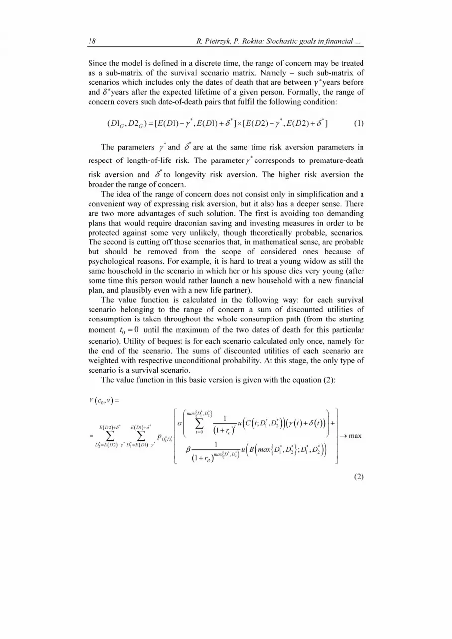
18 R. Pietrzyk, P. Rokita: Stochastic goals in financial …
Since the model is defined in a discrete time, the range of concern may be treated as a sub-matrix of the survival scenario matrix. Namely – such sub-matrix of scenarios which includes only the dates of death that are between �∗years before and �∗years after the expected lifetime of a given person. Formally, the range of concern covers such date-of-death pairs that fulfil the following condition:
* * * *
( 1 , 2 ) [ ( 1) , ( 1) ] [ ( 2) , ( 2) ]G G
D D E D E D E D E Dγ δ γ δ= − + × − + (1)
The parameters *γ and *
δ are at the same time risk aversion parameters in
respect of length-of-life risk. The parameter *γ corresponds to premature-death
risk aversion and *δ to longevity risk aversion. The higher risk aversion the
broader the range of concern. The idea of the range of concern does not consist only in simplification and a
convenient way of expressing risk aversion, but it also has a deeper sense. There are two more advantages of such solution. The first is avoiding too demanding plans that would require draconian saving and investing measures in order to be protected against some very unlikely, though theoretically probable, scenarios. The second is cutting off those scenarios that, in mathematical sense, are probable but should be removed from the scope of considered ones because of psychological reasons. For example, it is hard to treat a young widow as still the same household in the scenario in which her or his spouse dies very young (after some time this person would rather launch a new household with a new financial plan, and plausibly even with a new life partner).
The value function is calculated in the following way: for each survival scenario belonging to the range of concern a sum of discounted utilities of consumption is taken throughout the whole consumption path (from the starting moment
00t = until the maximum of the two dates of death for this particular
scenario). Utility of bequest is for each scenario calculated only once, namely for the end of the scenario. The sums of discounted utilities of each scenario are weighted with respective unconditional probability. At this stage, the only type of scenario is a survival scenario.
The value function in this basic version is given with the equation (2):
( )
( )
( )
{ }
( )( )( ) ( ) ( )( )
( ) { }{ }( )( )( )
( )
* *
1 2
* *
1 2
* *
* * *
* *
*
2
1 2
1
,
* *
1 2
0
2 1
2
0
* * * *
1
1
2,
1 2
1; ,
1
1, ; ,
1
,
max
max D D
t
t c
D
E
D
max
D E D
D E D D
D
D
D
B
E
u C t D D t tr
p
u B max D D D D
V c v
r
δ δ
γ γ
α γ δ
β
+ +
= − = −
=
+ +
=
= →
+
+
∑∑ ∑
(2)

STATISTICS IN TRANSITION new series, Spring 2015
19
where:
0c – consumption rate at the moment 0,
0v – proportion of Person 1 investment in total one-period contribution of the
household (1 1 2, 1v v v v≡ = − ),
( ).u – utility function (the same in all segments of the formula), *
γ – premature death risk aversion parameter (the number of years that the household takes into consideration),
*δ – longevity risk aversion parameter (also interpreted as the number of
years),
( )tγ – premature death risk aversion measure (depends on *γ ),
( )tδ – longevity risk aversion measure (depends on *δ ),
* *
1 2D D
p – (unconditional) probability of such scenario that
( )* *
1 21 , 2 ,D D D D= =
α – consumption preference, β – bequest preference,
Cr – discount rate of consumption,
Br – discount rate of bequest,
{ }* *
1 2, max D D – time of household end under the scenario of
( )* *
1 21 , 2D D D D= = ,
( )* *
1 2; ,C t D D – consumption at the moment t in the ( )* *
1 2,D D scenario,
( )* *
1 2; ,B t D D – cumulated investments and surplus of both household
members at the moment t in the ( )* *
1 2,D D scenario; for
{ }* *
1 2, t max D D= this is just amount of available bequest.
5.2. Augmenting the model by stochastic childbirth time
Let us assume that a pair is planning two children. They think of some time as the best for the first and the second child's birth, but certainly the true time of birth does not depend only on their decision. It is a random variable, conditional on the planned time.
The model with the Type I goals (2 children) is constructed using the same concept of a discrete grid of scenarios as in the previous subsection. The difference is that there is a number of childbirth scenarios put on each survival scenario. The range of possible the first child's births is from the start of the plan (

20 R. Pietrzyk, P. Rokita: Stochastic goals in financial …
00t = ) until the date of death of the woman in a given survival scenario, the
second child's birth dates are between the first child's birth until the scenario end for the woman. Any number of children may be added to the model in this way, but here it is limited to only two for simplicity. The probabilities attached to each childbirth scenario are taken from the distribution of conditional childbirth times discussed in section 4, subsection 4.2.
The value function formula used in this variant of the model is as presented in the equation (3):
( )
( )
( ) ( )
{ }
( )( )( ) ( ) ( )( )
( ) { }{ }( )( )
( )
* *
1 2
* * * **1 2 1 2
*
* *
1 2
* *
*01
1 2
,
*
0
, ,1
1 2
1 2 11
,
*
1 2
0
* * * *
1 2 1 2
1; , , 1, 2
1
1, ; , , 1, 2
1
,
max D D
t
t c
D D
m
W D D W D DE D
Ch Ch
Ch t Ch Ch
ax D
D D E D
D
B
u C t D D Ch Ch t tr
p
u B max D D D D Ch C
V c v
p
h
r
δ
γ
α γ δ
β
+
== −
=
=
+ + +
=
+
∑ ∑ ∑∑
( )
( ) *
* *
2
2
2
max
E D
E D
δ
γ
+
= −
→∑
(3)
where:
( )* *
1 2,W D D – time of death of the woman,
1Ch – time of the first child's birth, 2Ch – time of the second child's birth,
1 2Ch Chp – probability of a scenario of child 1 and child 2 time births.
In addition to the new set of scenarios, a modification is also needed in the functions calculating consumption and cumulated wealth that may be bequeathed. Both these functions take two more arguments now, namely – dates of children's births.
5.3. Type III goal in the model
As it has been assumed in section 4, time of realization of goal type III is deterministically dependent on the child's birth. Thus, the only new set of scenarios that would have to be taken into account is the price of the intended purchase. It is natural to treat the price as a continuous random variable, which leads to an infinite number of scenarios. Fortunately, the direction of price influence on the general financial situation of the household is known and pretty obvious. At the time when the household intends to buy a residential real estate, it is the better the lower the market price, and the higher the price – the worse. And inversely, at the moment when the house becomes a part of wealth to be bequeathed, the higher market price the better, and the lower price the worse.
Let aversion to real-estate price risk in respect of the type III goal be expressed in terms of a tolerance level. The tolerance level, by analogy to VaR or CFaR tolerance levels, is here understood as a significance indicating the

STATISTICS IN TRANSITION new series, Spring 2015
21
accepted probability of adverse scenarios. Here, it is some small pre-defined probability that a scenario of real estate prices will fall out of the range of scenarios for which the financial plan gives protection. Put differently, the household wants the plan to be optimized and meet budget and other constraints for at least all other scenarios.
For a tolerance level q , two quantile-based scenarios are considered. The first, for the moment of purchase. It is a right-tail quantile of real estate price distribution, corresponding to probability1 q− . The distribution used here is
unconditional (conditional on the state form the moment 0
0t = ) price distribution for the moment of purchase. The second, for the moment of bequest, is a conditional left-tail quantile corresponding to probability q , conditional on the upper quantile from the moment of purchase.
Let us assume that no new (larger) house nor any house expanding is planned when the second and next children are born.
The value function taking into account type III goal is given by the eq. (4):
( )
( )
( ) ( )
{ }
( )( )( ) ( ) ( )( )
( ) { } { }( )( )
( )
* *
1 2
* *
* * * **1 2 1 2
*1 2
*
0
*
1
*
1
2
,
* *
1 2 1
0
0
; ;1
1 2
1 2 11** * *
,
*
1 2 1 2 1
1; , , 1, 2,
1
1, ; , , 1, 2, ,
1
,
max D D
qtt c
W D D W D D
D D
qmax D
E D
Ch Ch
Ch t Ch C
D
B
hD E D
q
u C t D D Ch Ch S t
V c v
p
S
tr
p
u B max D D D D Ch Ch S
r
δ
γ
α γ δ
β
−
=
−
+
= == −
=
+ + +
+
∑∑ ∑ ∑
( )
( ) *
* *
2
2
2
max
E D
D E D
δ
γ
+
= −
→
∑
(4)
where: ( )1
11 ;q S hS F q T
−
−
= − ,
( )1
(
* 1
);
h qBS TS SqS F q T
−=
−
= ,
1h hT Ch= +∆ .
* *
1 2max{ , }
BT D D= . The ( )1
11 ;q S hS F q T
−
−
= − denotes unconditional quantile of real estate price
distribution at the moment hT for probability 1 q− .
( )1
(
* 1
);
h qBS TS SqS F q T
−=
−
= denotes quantile corresponding to probability q of
the conditional real estate price distribution at the moment BT , conditional on the
price at the moment hT being equal to
1 qS
−
.
Moreover, consumption and bequest functions take on new arguments.

22 R. Pietrzyk, P. Rokita: Stochastic goals in financial …
Consumption function depends now on the price of the real estate at the moment of purchase (
hT ). The wealth to be bequeathed depends also on the price
of purchase at the moment hT , because it influences consumption and thus also
cumulated surplus. But in addition to that, bequest depends also on the price at the moment
BT , since it is a part of the residual wealth.
In practice, the risk aversion of the household in this respect may be calibrated on the basis of the maximum price of a real estate (given standard, technical state and location) the decision makers would accept to pay in the future and the minimum price they would accept when selling it then. Of course, the prices would need to be brought to present values as of the time when the plan is prepared. Otherwise, household members would not have a feeling of weather they are high or low in real sense. Then, probabilities might be calculated for the decision maker automatically in the planning system to translate the input into terms used in the model.
6. Summary
The proposed concept of the household financial plan model takes into account a source of uncertainty that is hardly ever addressed in the personal finance literature. Other stochastic factors, like survival of the household members, returns on investments, interest rates of credits, labour income, health condition, or events of insurance type (both life and non-life) are covered by many models, though usually not all of them together at the same time. Here, in turn, the time of goal realization and the magnitude of some chosen goals is discussed and an attempt to identify and review their main statistic properties is made. Also, relationships between goals, both in the sense of statistical dependence and causal links, are generally discussed. As a result “child-birth-time driven” model of household financial planning is obtained.
The model at its present version of development is a proposition of theoretic concept, still based on a number of unverified assumptions and dependent on parameters that have not yet been estimated. And in the case of conditional distribution of a child's birth under the condition of the planned time, no type of distributions (nor even a family) have been specified yet. Also the choice of links between financial goals is made arbitrary, though on the ground of some life experience, and logical reasoning. Empirical research may change somewhat the structure of the goal dependency map.
Further research, besides solving technical problem of this version of the model, will concentrate on augmenting it by other stochastic elements. Particularly, the risk factors connected with financing the goals need to be modelled.
Also, an important issue that has not yet been taken into account in this model is a trade-off between life insurance and capital-based protection against

STATISTICS IN TRANSITION new series, Spring 2015
23
unexpected events in the area of survival process (Ibbotson et al. 2005, Huang et al., 2008).
Another question that may be taken up in further research is including different possible retirement goal realizations. In the accumulation phase different pension plans may be compared and selected (Blake et al., 2001). In the distribution phase different mixes of life annuity and asset fund may be used, plus some additional solutions (Blake et al., 2003; comp. also: Huang and Milevsky 2011; Milevsky and Huang 2011; Gong, Webb 2008). For a two-person household also a joint annuity variant, of the kind discussed by Brown and Poterba (2000), is worth considering.
Acknowledgement
The research project was financed by The National Science Centre (NCN) grant, on the basis of the decision no. DEC-2012/05/B/HS4/04081.
REFERENCES
ANDO, A., MODIGLIANI, F., (1957). Tests of the Life Cycle Hypothesis of Saving: Comments and Suggestions. Oxford Institute of Statistics Bulletin, Vol. XIX (May), pp. 99−124.
BLAKE, D., CAIRNS A., DOWD, K., (2001). Pensionmetrics: Stochastic Pension Plan Design During the Accumulation Phase. Insurance: Mathematics and Economics, Vol. 29, Issue 2, pp. 187−215.
BLAKE, D., CAIRNS A., DOWD, K., (2003). Pensionmetrics 2: Stochastic Pension Plan Design During the Distribution Phase. Insurance: Mathematics and Economics, Vol. 33, issue 1, pp. 29−47.
BODIE, Z., TREUSSARD, J., WILLEN, P., (2008). The Theory of Optimal Life-Cycle Saving and Investing. In: Z. Bodie, D. McLeavy, L.B. Siegel, eds., The Future of Life-Cycle Saving and Investing. The research Foundation of CFA.
BROCKETT, P. L., (1984). General bivariate Makeham laws. Scandinavian Actuarial Journal, Vol. 1984, Issue 3, pp. 150−156.
BROWN, J. R., POTERBA J. M., (2000). Joint Life Annuities And Annuity Demand By Married Couples, Journal of Risk and Insurance, 2000, 67(4), pp. 527−553.
BRUHN K., STEFFENSEN M., (2010). Household consumption, investment and life insurance. Insurance: Mathematics and Economics, 48, pp. 315−325.

24 R. Pietrzyk, P. Rokita: Stochastic goals in financial …
CARRIERE, J. F., (2000). Bivariate Survival Models for Coupled Lives. Scandinavian Actuarial Journal, 2000:1, pp. 17−32.
COX, J.C., HUANG, CH., (1989). Optimal consumption and portfolio policies when asset prices follow a diffusion process. Journal of Economic Theory, Vol. 49, Issue 1, pp. 33−83.
FELDMAN, L., PIETRZYK, R., ROKITA, P., (2014a). A practical method of determining longevity and premature-death risk aversion in households and some proposals of its application. In: M. Spiliopoulou, L. Schmidt-Thieme, R. Janning, eds., Data Analysis, Machine Learning and Knowledge Discovery. Studies in Classification, Data Analysis and Knowledge Organization. Berlin-Heidelberg: Springer, pp. 255−264.
FELDMAN, L., PIETRZYK, R., ROKITA, P., (2014b). Multiobjective optimization of financing household goals with multiple investment programs. Statistics in Transition, New Series, Spring, Vol. 15, No. 2, pp. 243−268.
FELDMAN, L., PIETRZYK, R., ROKITA, P., (2014c). Cumulated Surplus Approach and a New Proposal of Life-Length Risk Aversion Interpretation in Retirement Planning for a Household with Two Decision Makers (November 6, 2014). Available at SSRN: <http://ssrn.com/abstract=2473156>.
GEORGES, P., LAMY, A.-G., NICOLAS, E., QUIBEL, G., RONCALLI, T, (2001). Multivariate Survival Modelling: A Unified Approach with Copulas (May 28, 2001). Available at SSRN: <http://ssrn.com/abstract=1032559> [Version: 28 May 2001. Accessed: 04 Dec. 2014].
GEYER, A., HANKE, M., WEISSENSTEINER, A., (2009). Life-cycle asset allocation and consumption using stochastic linear programming. The Journal of Computational Finance, 12(4), pp. 29−50.
GHYSELS, E., PLAZZI, A., TOROUS, W. N., VALKANOV, R. I., (2012). Forecasting Real Estate Prices. In: G. Elliott, A. Timmermann, eds., Handbook of Economic Forecasting. Vol. II, Elsevier.
GOMPERTZ, B., (1825). On the Nature of the Function Expressive of the Law of Human Mortality, and on a New Mode of Determining the Value of Life Contingencies. Philosophical Transactions of the Royal Society of London, 115, 513−585.
GUTÍERREZ, R., GUTÍERREZ-SANCHEZ, R., NAFIDI, A., (2008). A bivariate stochastic Gompertz diffusion model: statistical aspects and application to the joint modeling of the Gross Domestic Product and CO2 emissions in Spain. Environmetrix Vol. 19, Issue 6, pp. 643−658.
GONG, G., WEBB, A., (2008). Mortality Heterogeneity and the Distributional Consequences of Mandatory Annuitization. The Journal of Risk and Insurance, 75(4), pp. 1055−1079.

STATISTICS IN TRANSITION new series, Spring 2015
25
HUANG, H., MILEVSKY, M. A., (2011). Longevity Risk Aversion and Tax-Efficient Withdrawals. [online] SSRN.
Available at: <http://ssrn.com/abstract=1961698> [Accessed: 22 March 2012].
HUANG, H., MILEVSKY, M. A., WANG, J., (2008). Portfolio Choice and Life Insurance: The CRRA Case. Journal of Risk & Insurance, Vol. 75, Issue 4, pp. 847−872.
IBBOTSON, R. G., CHEN, P., MILEVSKY, M. A., ZHU, X., (2005). Human Capital, Asset Allocation, and Life Insurance. Yale ICF Working Paper No. 05-11. Available at SSRN: <http://ssrn.com/abstract=723167>.
KONICZ, A. K., PISINGER, D., RASMUSSEN, K. M., STEFFENSEN, M., (2014). A Combined Stochastic Programming and Optimal Control Approach to Personal Finance and Pensions. Available at SSRN: <http://ssrn.com/abstract=2432869> [Version: 30 April 2014. Accessed: 24 Nov. 2014].
KOTLIKOFF, L. J., SPIVAK, A., (1981). The Family as an Incomplete Annuities Market. Journal of Political Economy, Vol. 89, No. 2, (April 1981), pp. 372−391.
MERTON, R. C., (1969). Lifetime portfolio selection under uncertainty: The continuous time case. The Review of Economics and Statistics, 51(3), pp. 247−257.
MERTON, R. C., (1971). Optimum consumption and portfolio rules in a continuous-time model. Journal of Economic Theory, 3(4), pp.373−413.
MILEVSKY, M. A., HUANG, H., (2011). Spending Retirement on Planet Vulcan: The Impact of Longevity Risk Aversion on Optimal Withdrawal Rates. Financial Analysts Journal, 67(2), pp. 45−58.
MODIGLIANI, F., BRUMBERG, R. H., (1954). Utility analysis and the consumption function: an interpretation of cross-section data. In: Kenneth K. Kurihara, ed. 1954. Post-Keynesian Economics. New Brunswick, NJ: Rutgers University Press, pp.388−436.
OHNISHI, T., MIZUNO, T., SHIMZU, CH., WATANABE, T., (2011). The Evolution of House Price Distribution. RIETI Discussion Paper Series 11-E-019. Available at <http://www.rieti.go.jp/jp/publications/dp/11e019.pdf> [Accessed: 04 Dec. 2014].
PIETRZYK, R. A., ROKITA, P. A., (2014). Facilitating Household Financial Plan Optimization by Adjusting Time Range of Analysis to Life-Length Risk Aversion (October 22, 2014).
Available at SSRN: <http://ssrn.com/abstract=2513393>.

26 R. Pietrzyk, P. Rokita: Stochastic goals in financial …
RICHARD, S. F., (1975). Optimal consumption, portfolio and life insurance rules for an uncertain lived individual in a continuous time model. Journal of Financial Economics, 2, pp. 187−203.
RUSZCZYŃSKI, A., SHAPIRO, A., (2003). Stochastic Programming Models. In: Ruszczyński, A., Shapiro, A., eds, Handbooks in Operations Research and Management Science, 10: Stochastic Programming, pp. 1−64.
VICKSON, R. G., ZIEMBA, W. T., eds, (2006). Stochastic Optimization Models in Finance. World Scientific.
WILLCOCKS, G., (2009). UK Housing Market: Time Series Processes with Independent and Identically Distributed Residuals. Journal of Real Estate Finance and Economics, Vol. 39, No. 4, 2009, pp. 403−414.
YAARI, M. E., (1965). Uncertain Lifetime, Life Insurance and Theory of the Consumer. The Review of Economic Studies, 32(2), pp.137−150.
ZALEGA, T., (2007). Gospodarstwa domowe jako podmiot konsumpcji (Households as consuming actors) (in Polish). Materials and Studies, Faculty of Management, University of Warsaw.
ZIEMBA, W. T., (2003). The Stochastic Programming Approach to Asset, Liability, and Wealth Management. The Research Foundation of AIMR™.


