Stochastic inversion of seismic PP and PS data for reservoir parameter estimation

1

Stochastic inversion of seismic PP and PS data for reservoir parameter 1

estimation 2

Jinsong Chen1, and Michael E. Glinsky2 3

4

Right Running Head: Stochastic inversion of PP and PS data 5

6

1Lawrence Berkeley National Laboratory, Earth Sciences Division, Berkeley, California 7

E-mail: [email protected] 8

9

2ION Geophysical, Houston, Texas 10

E-mail: [email protected] 11

12

13

2

ABSTRACT 1

We investigate the value of isotropic seismic converted-wave (i.e., PS) data for reservoir 2

parameter estimation using stochastic approaches based on a floating-grain rock physics 3

model. We first perform statistical analysis on a simple two-layer model built on actual 4

borehole logs and compare the relative value of PS data versus AVO gradient data for 5

estimating floating-grain fraction. We find that PS data are significantly more informative 6

than AVO gradient data in terms of likelihood functions, and the combination of PS and 7

AVO gradient data together with PP data provides the maximal value for the reservoir 8

parameter estimation. To evaluate the value of PS data under complex situations, we 9

develop a hierarchical Bayesian model to combine seismic PP and PS data and their 10

associated time registration. We extend a model-based Bayesian method developed 11

previously for inverting seismic PP data only, by including PS responses and time 12

registration as additional data and PS traveltime and reflectivity as additional variables. 13

We apply the method to a synthetic six-layer model that closely mimics real field 14

scenarios. The case study results show that PS data provide more information than AVO 15

gradient data for estimating floating-grain fraction, porosity, net-to-gross, and layer 16

thicknesses when their corresponding priors are weak. 17

18

3

INTRODUCTION 1

Multicomponent seismic surveying has been used for hydrocarbon exploration for 2

decades because it can capture the seismic wave-field more completely than conventional 3

single-element techniques (Stewart et al., 2002). Although several types of energy 4

conversion may occur when seismic waves pass through the underlying earth, transmitted 5

or multiple conversions generally have much lower amplitudes than the P-down and S-up 6

reflection (Rodriguez-Saurez, 2000). Consequently, among many applications of multi-7

component seismic data, the use of converted-wave or PS images receives much more 8

attention (Stewart et al., 2002; Mahmoudian and Margrave, 2004; Veire and Landro, 9

2006). However, the high acquisition cost of collecting multicomponent seismic data 10

compared to conventional seismic surveys and the challenge in processing 11

multicomponent data, makes the use of converted-wave data as a routine practice 12

difficult. 13

The interest in using multicomponent seismic data again for hydrocarbon 14

applications is inspired by recent advances in seismic data acquisition technologies, such 15

as ocean-bottom seismometer techniques (e.g., ocean-based cables and ocean-based 16

nodes) (Hardage et al., 2011; Pacal, 2012). With the use of new techniques, 17

multicomponent seismic data can be collected more reliably compared to conventional 18

seismic survey techniques. Another major reason for using multicomponent seismic data 19

is the need to estimate spatially-distributed ductile fraction (Glinsky et al., 2013), and to 20

characterize fractures for unconventional resources because shear-wave splitting provides 21

an effective approach to image fracture orientation and density (Bale et al., 2013). There 22

are many other successful applications of converted-wave data, such as time-lapse 23

4

monitoring of geomechanical changes (Davis et al., 2013), and reservoir characterization 1

(Brettwood et al., 2013). 2

In this study, we use stochastic approaches to investigate the value of converted-3

wave data for reservoir parameter estimation based on a floating-grain rock physics 4

model developed by DeMartini and Glinsky (2006). The model is well-documented in 5

Gunning and Glinsky (2007) and appropriate for porous sedimentary rocks in which 6

some solid materials are “floating” or not involved in loading support because it can 7

explain the observed variation in P-wave velocity versus density trends and the lack of 8

variation in the P-wave velocity versus S-wave velocity trends. The rock physics 9

relationship can be modified and applied to unconventional shale resource exploration as 10

done by Glinsky et al. (2013), where the media is considered as a binary mixing of brittle 11

and ductile materials and the ductile fraction plays the same role as the floating-grain 12

fraction in this model. 13

We employ stochastic methods in the study because they have many advantages 14

over traditional deterministic approaches in reservoir parameter estimation using multiple 15

geophysical data sets, especially when we deal with complex issues involving uncertainty 16

(Chen et al., 2008). We start from analyzing a simple two-layer model by comparing the 17

relative value of PS versus AVO gradient data for estimating floating-grain fraction 18

according to their likelihoods when both rock physics models and seismic data are 19

subject to uncertainty. We then focus on more complicated cases involving multiple 20

layers and develop a hierarchical Bayesian model to combine seismic PP and PS data and 21

their associated time registration. 22

5

We extend the model-based Bayesian method developed by Gunning and Glinsky 1

(2004) for inverting seismic PP data to allow isotropic converted-wave responses and PS 2

event time registration as additional data. We use the same rock physics models and 3

Markov chain Monte Carlo (MCMC) sampling strategies as Gunning and Glinsky (2004). 4

Since this study is built on the previous work, the subsequent descriptions will be focused 5

on the new development and applications; the details of other parts can be found in 6

Gunning and Glinsky (2004). 7

ROCK PHYSICS MODEL AND ANALYSIS OF TWO-LAYER MODELS 8

Floating-grain rock physics model 9

We use the floating-grain rock physics model developed by Demartini and Glinsky 10

(2006) and Gunning and Glinsky (2007) to link reservoir parameters to seismic attributes. 11

In the model, the subsurface is considered as a binary mixture of reservoir members (e.g., 12

sand) and non-reservoir members (e.g., shale). For sand, we assume that some solid 13

materials are “floating” in pore space and the seismic properties (i.e., seismic P- and S-14

wave velocity and density) can be characterized by two fundamental parameters: the 15

loading depth ( z ), which is a measure of effective pressure, and the floating-grain 16

fraction ( x ). The general model is given below 17

,p vp vp vp vpv a b z c x ε= + + + (1) 18

,s vs vs p vsv a b v ε= + + (2) 19

.pa b v c xρ ρ ρ ρρ ε= + + + (3) 20

6

In equations 1-3, pv , sv , and ρ are seismic P- and S-wave velocity and density, 1

respectively; vpa , vpb , vpc , vsa , vsb , ρa , ρb , and ρc are the fitting coefficients. Symbols 2

ε vp , εvs , and ρε represent uncertainty associated with the regression equations. We 3

assume that ε vp , εvs , and ρε have Gaussian distributions with zero mean and variance of 4

2σ vp , 2σ vs , and 2

ρσ , respectively. 5

We rewrite equations 2-3 in terms of loading depth z and floating-grain fraction x 6

as follows 7

( ) ( ),s vs vp vs vs vp vs vp vs vp vsv a a b b b z b c x b ε ε= + + + + + (4) 8

( ) ( ) ( ).vp vp vp vpa a b b b z b c c x bρ ρ ρ ρ ρ ρ ρρ ε ε= + + + + + + (5) 9

We can see that in the rock physics model, seismic properties linearly depend on the 10

reservoir parameters with uncertainty. 11

We can use different relationships for shale because seismic properties in shale do 12

not depend on floating-fraction. As it has been done in Gunning and Glinsky (2007), we 13

drop floating-grain fraction from equations 1 and 4 and use the power-law form of the 14

Gardner relationship (Gardner et al., 1974) for density, i.e., bpav ρρ ε= + , where a and b 15

are fitting coefficients. By fitting actual borehole logs from suitable field sites, we can 16

obtain all the needed coefficients and their associated standard errors for sand and shale 17

members. Table 1 is a summary of all those values. 18

Reflectivity coefficients 19

7

We use the linearized Zoeppritz approximations (Aki and Richard, 1980) for small 1

contrasts to obtain PP and PS reflectivity coefficients at an interface, which are given 2

below 3

2 2

2 2

1 1= 4 2 sin2 2

1 + sin tan ,2

p p spp sp p

p p s

pp p

p

v v vR rv v v

vv

ρ ρ θρ ρ

θ θ

⎛ ⎞ ⎡ ⎤Δ Δ ⎛ ⎞ΔΔ Δ+ + − +⎜ ⎟ ⎢ ⎥⎜ ⎟⎜ ⎟ ⎢ ⎥⎝ ⎠⎝ ⎠ ⎣ ⎦Δ

(6) 4

( )

( )

2 2

2 2

sin1 2 sin 2 cos cos

2cos2sin

+ sin cos cos .cos

pps sp p sp p s

s

p ssp p sp p s

s s

R r r

vr rv

θ ρθ θ θθ ρθ

θ θ θθ

Δ= − − +

Δ− (7) 5

In equations 6 and 7, 1 2( ) / 2p p pv v v= + , 1 2( ) / 2s s sv v v= + , 1 2( ) / 2ρ ρ ρ= + , /sp s pr v v= , 6

2 1p p pv v vΔ = − , 2 1s s sv v vΔ = − , and 2 1ρ ρ ρΔ = − , where ( 1pv , 1sv , 1ρ ) and ( 2pv , 2sv , 2ρ ) 7

are P-wave and S-wave velocity and density in the layers above and below the interface. 8

Symbols pθ and sθ are the P-wave and S-wave incident angles; they are connected 9

through Snell’s law as sin / sin /p p s sv vθ θ= . 10

Equation 6 is the same as the one used by Castagna et al. (1998), where the first 11

and second terms on the right side of the equation are referred to as AVO intercept and 12

gradient, respectively. The third term is high-order variations and dominated at far offsets 13

near the critical angle (Mavko et al., 1998). Equation 7 is the same as the one used by 14

Veire and Landro (2006). For ease of description, we let 0A be the AVO intercept, 1A be 15

all the terms on the right side of equation 7, and 2A be the AVO gradient with the high-16

order term. Let 17

https://www.researchgate.net/publication/215754828_Framework_for_AVO_gradient_and_intercept_interpretation?el=1_x_8&enrichId=rgreq-cbc7fb6d-5650-477b-add8-c371b8fbc87f&enrichSource=Y292ZXJQYWdlOzI2NTMzNTQyMjtBUzoxMzc3NDk4MjI3MDk3NjBAMTQwOTg1MzUyNTcyMA==

8

( )

( )

2 21

2 22

sin1 2 sin 2 cos cos , and

2cos

2sinsin cos cos .

cos

psp p sp p s

s

psp p sp p s

s

g r r

g r r

θθ θ θ

θθ

θ θ θθ

⎧= − − +⎪

⎪⎨⎪ = −⎪⎩

(8) 1

We have the following relationship 2

0

1 1 22 2 2 2 2 2

2

1/ 2 1/ 2 0 /0 / .

2 sin sin (1 tan ) / 2 4 sin /p p

sp p p p sp p s s

AA g g v vA r r v v

ρ ρ

θ θ θ θ

⎛ ⎞ Δ⎛ ⎞ ⎛ ⎞⎜ ⎟⎜ ⎟ ⎜ ⎟= Δ⎜ ⎟⎜ ⎟ ⎜ ⎟

⎜ ⎟ ⎜ ⎟⎜ ⎟− + − Δ⎝ ⎠ ⎝ ⎠⎝ ⎠

(9) 3

We use the capital letter A to represent the vector on the left side of equation 9 and use 4

aM and ΔC represent the matrix and the vector on the right side of the equation. Thus 5

equation 9 becomes a= ΔA M C. These notations will be used in the subsequent text. 6

Synthetic two-layer model 7

To demonstrate the value of PS data, we start from a simple two-layer model based 8

on actual borehole logs from Gunning and Glinsky (2007), with the first layer being shale 9

and the second layer being sand whose rock physics models are given in Table 1. Since 10

we focus on estimation of floating-grain fraction in the sand layer, we fix the loading 11

depth as 1 5,200z = m and 2 5,321z = m for the first and second layers. By using the 12

shale regression equations with coefficients given in Table 1, we have 1 3, 279pv = m/s, 13

1 1,596sv = m/s, and 1 2.50ρ = g/cc. By using equations 1, 4, and 5, we get 14

2 1( ) ( ) ( ),vp vp vp vpa a b b b z b c c x bρ ρ ρ ρ ρ ρ ρρ ρ ε εΔ = + + − + + + + (10) 15

2 1( ) ,p vp vp p vp vpv a b z v c x εΔ = + − + + (11) 16

2 1( ) ( ).s vs vp vs vp vs s vs vp vs vs vpv a a b b b z v b c x bε εΔ = + + − + + + (12) 17

9

Let 1

2 1

2 1

2 1

vp vp

vp vp vp p

vs vs vp vs vp vs s

w a a b b b zw a b z vw a a b b b z v

ρ ρ ρ ρ ρ⎧ = + + −⎪ = + −⎨⎪ = + + −⎩

(13) 2

We have 3

/ / ( ) / ( ) // / / / ./ / / ( ) /

vp vp

p p vp p vp p vp p

s s vs s vs vp s vs vs vp vs

w c b c bv v w v c v x vv v w v b c v b v

ρ ρ ρ ρ ρρ ρ ρ ρ ε ε ρε

ε ε

⎛ ⎞ ⎛ ⎞Δ + +⎛ ⎞ ⎛ ⎞⎜ ⎟ ⎜ ⎟⎜ ⎟ ⎜ ⎟Δ = + +⎜ ⎟ ⎜ ⎟⎜ ⎟ ⎜ ⎟

⎜ ⎟ ⎜ ⎟ ⎜ ⎟ ⎜ ⎟Δ +⎝ ⎠ ⎝ ⎠ ⎝ ⎠ ⎝ ⎠

(14) 4

Let 0W , 1W , and wε represent the first, second, and third vectors on the right side of 5

equation 14; thus, we have 0 1 .wxΔ = + +C W W ε By assuming that the errors in equations 6

1-3 are independent, we can obtain the following covariance matrix wΣ 7

2 2 2 2 2 2

2 2 2 2

2 2 2 2 2 2

( ) / / ( ) / ( )/ ( ) / / ( ) ./ ( ) / ( ) ( ) /

vp vp p vs vp s

w vp p vp p vs vp p s

vs vp s vs vp p s vs vs vp vs

b b v b b vb v v b v vb b v b v v b v

ρ ρ ρ ρ

ρ

ρ

σ σ ρ σ ρ σ ρσ ρ σ σσ ρ σ σ σ

⎛ ⎞+⎜ ⎟∑ = ⎜ ⎟⎜ ⎟+⎝ ⎠

(15) 8

Synthetic seismic data and likelihood function 9

For the purpose of this analysis, we consider both PP and PS reflectivities at the 10

interface as data even if they often are unknown and estimated from full waveform 11

seismic responses in practice. Specifically, we use a PP trace with a zero incident angle 12

(i.e., 0A ), a PS trace with the P-wave incident angle of 45 degrees (i.e., 1A ), and an AVO 13

gradient trace (including the high-order term) with the P-wave incident angle of 45 14

degrees (i.e., 2A ). Let vector mR be the data with additive Gaussian random noise mε ; 15

we thus have 16

0 1( ) ( )m d m d a m d a m d a wx= + = Δ + = + + +R M A ε M M C ε M M W W ε M M ε , (16) 17

10

where dM is referred to as a data matrix that determines which types of data are used for 1

analysis (see Appendix A). 2

The second term on the right side of equation 16 is residuals; they include 3

measurement errors in seismic data and uncertainty caused by rock physics models. Since 4

both measurement errors and uncertainty in rock physics models are assumed to have 5

multivariate Gaussian distributions, their summation also has a multivariate Gaussian 6

distribution (Stone, 1995). Let mΣ be the covariance matrix of the measurement errors 7

and wΣ be the covariance matrix of the uncertainty in rock physics models. The 8

combined covariance thus is given by ( ) ( )Tc m d a w d a∑ = ∑ + ∑M M M M , where wΣ is 9

given by equation 15. Consequently, the likelihood function of x given data mR is a 10

multivariate Gaussian distribution as follows 11

{ }

1/2

10 1 0 1

( | )

exp ( ) ( ) .m c

Tm d a d a c m d a d a

f x

x x

−

−

∝ ∑

× − − − ∑ − −

R

R M M W M M W R M M W M M W (17) 12

Model comparison 13

We compare the estimation results obtained by using four combinations of seismic 14

data by specifying the data matrices: (1) using the PP data only, (2) using the PP and PS 15

data, (3) using the PP and AVO gradient data, and (4) using all the seismic data (see 16

Appendix A). Their corresponding data are represented by (1)mR , (2)

mR , (3)mR , and (4)

mR . To 17

avoid the effects of prior distribution on floating-grain fraction, we focus on the 18

likelihood functions ( )( | )kmf xR ( 1,2,3, and 4k = ) for those models. 19

Figure 1 compares the likelihood functions for the true floating-grain fraction being 20

0.0 (Figure 1a) and 0.035 (Figure 1b). The noise levels for all the data are equal to 0.01 in 21

11

the unit of reflection coefficients (RFC). As we expect, the true values have the 1

maximum likelihood in both cases. It is clear that the likelihoods of using the PP and 2

AVO gradient data are considerably larger than those of using the PP data only. The 3

likelihoods of using the PP and PS data are significantly larger than those of using the PP 4

and AVO gradient data. This suggests that the combination of the PP and PS data are 5

more informative for estimating floating-grain fraction than the combination of the PP 6

and AVO gradient data. When we use all the data, we get the largest likelihoods. This 7

implies that the PS and AVO gradient data might complement each other to some degree. 8

In addition, we can see that the clean sand (i.e., 0x = , see Figure 1a) overall has larger 9

likelihoods than the sand with floating grain (i.e., 0.035x = , see Figure 1b). 10

The above comparison may depend on noise levels in the seismic data. In practice, 11

PS and AVO gradient data typically have larger errors than PP data. To investigate the 12

effects of noise on the likelihood analysis, we vary noise levels in both PS and AVO 13

gradient data from 0.01 RFC to 0.1 RFC while still fixing the noise level of the PP data as 14

0.01 RFC. We first calculate the maximum likelihoods for each combination of seismic 15

data and then normalize the results by the values of using the PP data only to get the 16

following likelihood ratios 17

( )

(1)

max{ ( | )}.max{ ( | )}

km

km

f xrf x

= RR

(18) 18

Figure 2 shows the likelihood ratios for the true floating-grain fraction of 0.0 and 19

0.035. Generally, as the noise levels in the PS and AVO gradient data increase, the 20

likelihood ratios decrease and approach 1, the result of using the PP data only. 21

Additionally, the likelihood ratios of using the PP and PS data always have larger 22

likelihood ratios than those of using the PP and AVO gradient data; the likelihood ratios 23

12

of using all the data always have the largest values. This suggests that the combination of 1

PP and PS data is more informative than that of PP and AVO gradient data even under 2

large noise levels. 3

BAYESIAN MODEL FOR MULTIPLE LAYERS 4

Hierarchical Bayesian models 5

Although analysis of two-layer models allows us to understand the value of PS data 6

for floating-grain fraction estimation, it is marginal analysis of relative changes of 7

compaction and floating-grain fraction across an interface under simple conditions. In the 8

case of multiple layers, we need to develop a hierarchical Bayesian model to combine 9

seismic PP and PS data and their time registration. This model is an extension of the 10

model-based Bayesian method by Gunning and Glinsky (2004) with converted wave 11

responses and PS time registration as additional data and PS traveltime and reflectivity as 12

additional unknowns. 13

We consider effective seismic P-wave and S-wave velocity ( pv and sv ) and 14

density (ρ ), and seismic PP and PS reflectivity ( ppR and psR ) as unknowns. They are 15

functions of rock physics parameters through suitable rock physics models. We consider 16

PP traveltime ( ppt ) as a primary unknown; both layer thickness (d ) and PS traveltime (17

pst ) can be derived from the PP traveltime and associated effective seismic attributes. 18

The data used for inversion include seismic PP and PS full-waveforms ( ppS and psS ) and 19

PP and PS event registration time ( ppT and psT ). If available, we can also include other 20

types of information from nearby boreholes, such as depth constraints ( bD ). 21

13

Figure 3 shows all the unknowns, available data, and their relationships; the dashed 1

rectangle highlights our extension to the method by Gunning and Glinsky (2004). 2

Specifically, we add two unknowns related to converted wave (i.e., pst , and psR ) and 3

two types of new data sets (i.e., psT and psS ). Following the direct graphical model, we 4

have the following hierarchical Bayesian model: 5

( , , , , , , , , | , , , , )

( | , ) ( | , ) ( | )

( | ) ( | ) ( | , , )

( | , , ) ( | , ) ( | , , )

( , , | ) ( ) ( ).

pp ps p s pp ps pp ps pp ps b

pp pp pp ps ps ps pp pp

ps ps b pp p s

ps p s pp p ps pp p s

p s pp

ff f ff f ff f ff f f

α t t d v v ρ R R S S T T DS t R S t R T tT t D d R v v ρR v v ρ d t v t t v vv v ρ α α t

∝

×

×

×

(19) 6

Equation 19 defines a joint posterior probability distribution function of all 7

unknown parameters up to a normalizing constant. The first five terms on the right side of 8

the equation are the likelihood functions of available data, which link data to the 9

associated unknowns; other terms on the right side are the prior probability distributions, 10

which are derived from other sources of information, such as rock physics models. We 11

define all the likelihood functions and prior distributions in a similar way to the method 12

of Gunning and Glinsky (2004). In the following, we only describe the new development. 13

Equation 19 is a general Bayesian model for combining seismic PP and converted-14

wave data; we can simplify or vary the equation in different ways depending on specific 15

applications. For example, we can consider PP and PS reflectivities as functions of pv , 16

sv , and ρ , but ignore their associated uncertainties. We can also consider depth d as a 17

function of P-wave velocity and PP traveltime. Since in Bayesian statistics (Bernardo and 18

Smith, 2000), data affect unknowns only through likelihood functions, we can use some 19

14

statistics ( , )pp psQ S S of seismic data ppS and psS in the Bayesian model, for example, 1

the rotation and truncation of original seismic data through principal component analysis 2

(Venables and Ripley, 1999) or other methods. Consequently, we can have the following 3

Bayesian model 4

( , , , , , | , , , )

( | , , , , ) ( | ) ( | )

( | , , ) ( , , | ) ( ) ( ).

pp ps p s pp ps pp ps

pp ps p s pp pp ps ps

ps pp p s p s pp

ff f ff f f f

∝

×

α t t v v ρ S S T TQ t t v v ρ T t T tt t v v v v ρ α α t

(20) 5

Likelihood function of seismic data 6

We describe a general form of the likelihood function in terms of statistics of 7

seismic data, with the likelihood function of original seismic data as a special case of the 8

form. Let ( , , , , )pp ps p sG t t v v ρ be the response vector of a suitable forward model that 9

links seismic statistics Q to unknowns. Let vector mε represent the residuals. We assume 10

that the residuals have the multivariate Gaussian distribution with zero mean and the 11

covariance matrix of mΣ ; thus, we have 12

( ) ( )

1/2/2

1

( | , , , , ) (2 )

1 exp ( , , , , ( , , , ,2

kpp ps p s m

T

pp ps p s m pp ps p s

f π −−

−

= Σ

⎛ ⎞× − − Σ −⎜ ⎟⎝ ⎠

Q t t v v ρ

Q G t t v v ρ Q G t t v v ρ . (21) 13

In equation 21, k is the dimension of the multivariate Gaussian distribution and mΣ is 14

the determinant of the covariance matrix mΣ . One of the main advantages of using 15

statistics in equation 21 is that we can have more options in defining likelihood functions 16

so that we can make their residuals uncorrelated. 17

Likelihood functions of PP and PS event time registration 18

15

The use of event time registration as data is one of the main advantages of the 1

method by Gunning and Glinsky (2004), as well as the current extension, because PP 2

event time is directly related to P-wave velocity and PS event time directly related to P-3

wave and S-wave velocity. They provide additional information to constrain the estimates 4

of P-wave and S-wave velocity beyond the reflectivity-based PP and PS full-waveforms. 5

Traditional methods for joint inversion of PP and PS data are primarily based on 6

the mapping of PS data to PP time (or domain conversion), in which PS data are 7

considered as additional seismic stacks. Although this approach is simple to implement, it 8

suffers from difficulties, such as wavelet distortion (Bansal and Matheney, 2010), 9

because the conversion of PS time to PP time needs interval seismic P-to-S velocity 10

ratios, which are not known a-priori. 11

In this study, we avoid the PP-to-PS domain conversion and use PS data directly in 12

the PS time domain. We pick a PS event from PS seismograms that has a good 13

correspondence with a PP event in the PP seismograms along the same profile; we refer it 14

to as the master PS horizon. In the PS forward simulation, we calculate all the PS times 15

relative to the master horizon. The relative PP and PS time for a given layer is calculated 16

by 17

1 12

pps pp

s

Vt t

V⎛ ⎞

Δ = + Δ⎜ ⎟⎝ ⎠

. (22) 18

In equation 22, both pV and sV are interval velocities and are unknown; they will be 19

estimated in inversion procedures. 20

The likelihood functions of PP and PS event registration time are determined by 21

assuming that the errors have multivariate Gaussian distributions. Let Σ pp and Σ ps be the 22

https://www.researchgate.net/publication/241584576_Wavelet_distortion_correction_due_to_domain_conversion?el=1_x_8&enrichId=rgreq-cbc7fb6d-5650-477b-add8-c371b8fbc87f&enrichSource=Y292ZXJQYWdlOzI2NTMzNTQyMjtBUzoxMzc3NDk4MjI3MDk3NjBAMTQwOTg1MzUyNTcyMA==

16

covariance matrices of PP and PS event time, respectively. We have the following 1

likelihood functions 2

( ) ( )

( ) ( )

1

2

1/2/2 1

1/2/2 1

1( | ) (2 ) exp , and21( | ) (2 ) exp .2

Tkpp pp pp pp pp pp pp pp

Tkps ps ps ps ps ps ps ps

f

f

π

π

−− −

−− −

⎛ ⎞= Σ − − Σ −⎜ ⎟⎝ ⎠⎛ ⎞= Σ − − Σ −⎜ ⎟⎝ ⎠

T t T t T t

T t T t T t (23) 3

In equation 23, 1k and 2k are the dimensions of ppT and psT ; ppΣ and psΣ are the 4

determinants of the covariance matrix ppΣ and psΣ . 5

Conditionals of unknowns and Markov chain Monte Carlo sampling methods 6

We use Markov chain Monte Carlo methods to draw many samples from the joint 7

distribution given in equation 20. To do this, we first need to derive conditional 8

distributions of each type of unknowns given all other variables and data. The 9

normalizing constants of each conditional are irrelevant when we use MCMC methods to 10

draw samples. Therefore, we only need to keep the term on the right of equation 20 to get 11

its conditional, which are given below 12

( | ) ( | , , , , ) ( | ) ( | , , ) ( ),pp pp ps p s pp pp ps pp p s ppf f f f f⋅ ∝t Q t t v v ρ T t t t v v t (24) 13

( | ) ( | , , , , ) ( | ) ( | , , ),ps pp ps p s ps ps ps pp p sf f f f⋅ ∝t Q t t v v ρ T t t t v v (25) 14

( , , | ) ( | , , , , ) ( | , , ) ( , , | ),p s pp ps p s ps pp p s p sf f f f⋅ ∝v v ρ Q t t v v ρ t t v v v v ρ α (26) 15

( | ) ( , , | ) ( ).p sf f f⋅ ∝α v v ρ α α (27) 16

For equations 24-26, we cannot obtain analytical forms of those conditionals 17

because PP and PS registration time and seismic attributes ,pv sv , and ρ are nonlinear 18

17

functions of other variables. We have to use MCMC methods to draw many samples 1

from the joint posterior distribution. 2

In equation 27, we use the floating-grain rock physics model given in equations 1-3 3

to link layered seismic attributes to their corresponding reservoir parameters, which is a 4

linear function in this case. Let vector r be the combined vector of pv , sv , and ρ 5

arranged by the layer indices and vector α be the corresponding reservoir parameters. 6

We thus have r r= + +r µ Hα ε , where vector rε represents the uncertainty associated 7

with the linear relationship. We assume that it has a multivariate Gaussian distribution 8

with zero mean and the covariance matrix of rΣ . The detailed derivation and specific 9

forms are given in Appendix B. 10

If we use a multivariate Gaussian prior for α , i.e., ( ) ( , )p pf N Σα µ: , we can 11

obtain the analytical formula of posterior distribution, ( | ) ( , )u uf N⋅ Σα µ: , which is 12

given below 13

1 1 1

1 1 1

,

( ) .

Tu r p

Tu u r r p p

− − −

− − −

⎧Σ = Σ +Σ⎪⎨Σ = Σ − +Σ⎪⎩

H Hµ H r µ µ

(28) 14

We can obtain many samples of the joint posterior distribution given in equation 20 by 15

using MCMC sampling methods. 16

CASE STUDY OF MULTIPLE LAYERS 17

We use the second example of Gunning and Glinsky (2007) to demonstrate the 18

benefits of including converted-wave data into estimation of floating-grain fraction. 19

Figure 4 shows various logs from an actual borehole, including P-wave and S-wave 20

velocity, density, P-wave and S-wave velocity ratios, and P-wave impedance. According 21

18

to the logs, we can build a synthetic model with six layers, which are (1) hard marl, (2) 1

soft marl, (3) shale, (4) upper sand, (5) shale, and (6) lower sand, from shallow to deep 2

(see Figure 4). Both upper and lower sands are oil reservoirs with an oil saturation of 3

0.62, the net-to-gross of 0.65, and thicknesses of 213.4 m (or 700 ft) and 109.7 m (or 360 4

ft), respectively. Figure 5 shows the blockwise values of P-wave and S-wave velocity, 5

density, P-wave and S-wave velocity ratios, and P-wave impedance as a function of 6

normalized depth. As shown in the figure, layers 4 and 6 have relatively low Vp/Vs 7

ratios, both of which include the floating-grain fraction of 0.035. 8

PP and PS reflectivities and synthetic seismic data 9

We generate synthetic PP and PS data by first using equations 6 and 7 to calculate 10

PP and PS reflectivities and then convolve the reflectivities with a 30 Hz Ricker wavelet. 11

We consider P-wave incident angles of 0, 9, 18, 27, 36, and 45 degrees. Figure 6 shows 12

the synthetic seismic data without noise added, where PP data are in the PP time domain 13

but the PS data are in the PS time domain. For inversion, we consider the PP trace at the 14

incident angle of zero as PP data, and the PS traces at all the five incident angles as PS 15

data. We extract AVO gradient traces by subtracting the zero incident angle PP trace 16

from the PP traces with nonzero incident angles. We assume that all those data have 17

uncorrelated Gaussian random noise with the standard deviation of 0.01 RFC or 0.02 18

RFC, depending on synthetic cases. 19

Priors for the inversion 20

Since our main focus is on the demonstration of the value of PS data for reservoir 21

parameter estimation, we mainly focus on the estimation of floating-grain fraction and 22

net-to-gross in the upper and lower pay layers. Similar to Gunning and Glinsky (2007), 23

19

we first consider prior 2(0.02,0.03 )X N: ; this is a strong prior for the true floating-grain 1

fraction of 0.035. Secondly, we consider a weak prior 2(0.0,0.05 )X N: ; this give 2

significant prior probability to the zero floating-grain fraction or clean sand. For net-to-3

gross (NG), we also consider two types of priors: (1) 2~ (0.6,0.1 )NG N , and (2) 4

2~ (0.5,0.3 )NG N . 5

Since we use model-based inversion methods, we can set a wide range of priors and 6

consider many parameters as unknowns. For example, we assume that PP traveltime to 7

each interface has the normal distribution with the true values as mean and 10 8

milliseconds as the standard deviation. We assume that the uncertainty in the thickness of 9

layer 4 is 21.3 m (or 70 ft) (i.e., 10% of the thickness) and 6.1 m (or 20 ft) for other 10

layers. 11

Inversion cases 12

To test the usefulness of PS data for improving parameter estimation, we invert 13

synthetic seismic data under the following four scenarios: (1) using only the PP data, (2) 14

using PP and AVO gradient data, (3) using PP and PS data, and (4) using all the seismic 15

data. We compare the posterior estimates of unknowns under each case with their 16

corresponding prior distributions to evaluate the benefit of using PS data. 17

Since the above comparisons usually depend on inversion situation, we consider 18

the following three factors: (1) prior on floating-grain fraction (i.e., 2(0.02, 0.03 )X N: 19

or 2(0.0, 0.05 )X N: ), (2) prior on net-to-gross (i.e., 2(0.6, 0.1 )NG N: or 20

2(0.5, 0.3 )NG N: ), and (3) noise levels. We consider two sets of noise levels. The first 21

20

one is that all seismic data have a noise level of 0.01 RFC, and the other is that the PP 1

data has a noise level of 0.01 RFC but other data have a noise level of 0.02 RFC. 2

By changing priors and noise levels, we obtain many sets of posterior distributions. 3

We use MCMC methods to draw 20,000 samples and keep the later half for analysis (i.e., 4

10,000 samples). As an example, Figure 7 shows 200 realizations, selected from the 5

10,000 samples by keeping every 50th draw of the chain, for effective P-wave and S-wave 6

velocity and density along the profile in the case using strong priors (i.e., 7

2(0.02, 0.03 )X N: , and 2~ (0.6,0.1 )NG N ) and PP and PS data, where the red line 8

segments are their corresponding true values. Although those realizations are around the 9

true values, considerable uncertainties exist. With the use of those samples, we can obtain 10

wide ranges of statistics, such as means, medians, modes, density functions, and 11

predictive intervals. In the following several subsections, we selectively report our 12

inversion results. 13

Estimation of floating-grain fraction, porosity, and net-to-gross 14

We compare the estimates of reservoir parameters (i.e., floating-grain fraction, net-15

to-gross, and porosity) under different prior distributions. To investigate the effects of 16

priors about floating-grain fraction, we use a strong prior about net-to-gross, i.e., 17

2~ (0.6,0.1 )NG N , and noise levels for all the data types of 0.01 RFC. This implies the 18

same quality for all the seismic data. We will explore the effects of noise levels later on. 19

Figure 8 compares the posterior probability densities (PDFs) of floating-grain 20

fraction, porosity, and net-to-gross with their corresponding prior PDFs for layer 4 (i.e., 21

upper-pay layer). For floating-grain fraction, even under the good prior (i.e, 22

2~ (0.02,0.03 )X N ), the mode of the prior probability corresponds to the zero floating-23

21

grain fraction or clean sand. After conditioning to seismic data (i.e., PP data, PP plus 1

AVO data, or PP plus PS data), the modes of the posterior PDFs corresponds to the true 2

values 0.035, with the results of using PP and PS data fitting better than the other two. As 3

shown in Figure 9a, if we use a biased prior to clean sand, say 2~ (0.0,0.05 )X N , the 4

posterior estimates of floating-grain fraction using PP data only and using both PP and 5

AVO gradient data provide biased results (i.e., clean sand). However, the combination of 6

PP and PS data still provides correct estimates of the true value. 7

We can get similar results for comparison of porosity PDFs. Under the good prior 8

of floating-grain fraction, the modes of the posterior estimates for all the combinations of 9

seismic data correspond to the true value well (see Figure 8b). But under the biased prior 10

of floating-grain fraction, only the posterior estimates obtained using PP and PS data 11

provide good estimates of porosity (see Figure 9b). Since we use a very strong prior 12

about net-to-gross (i.e., 2~ (0.6,0.1 )NG N ) for the true value of 0.65, we expect the 13

updating of the prior to be minimal for all the posterior estimates (Figure 9c). 14

We have similar comparisons of posterior PDFs for the lower-pay layer (i.e., layer 15

6). As shown in Figure 10, although overall the posterior estimates of floating-grain 16

fraction and porosity are worse than those in the upper-pay layer, the combination of PP 17

and PS data provides more information than PP data only or the combination of PP and 18

AVO gradient data for updating the priors of floating-grain fraction and porosity. 19

Effects of the prior about net-to-gross and noise levels in seismic data 20

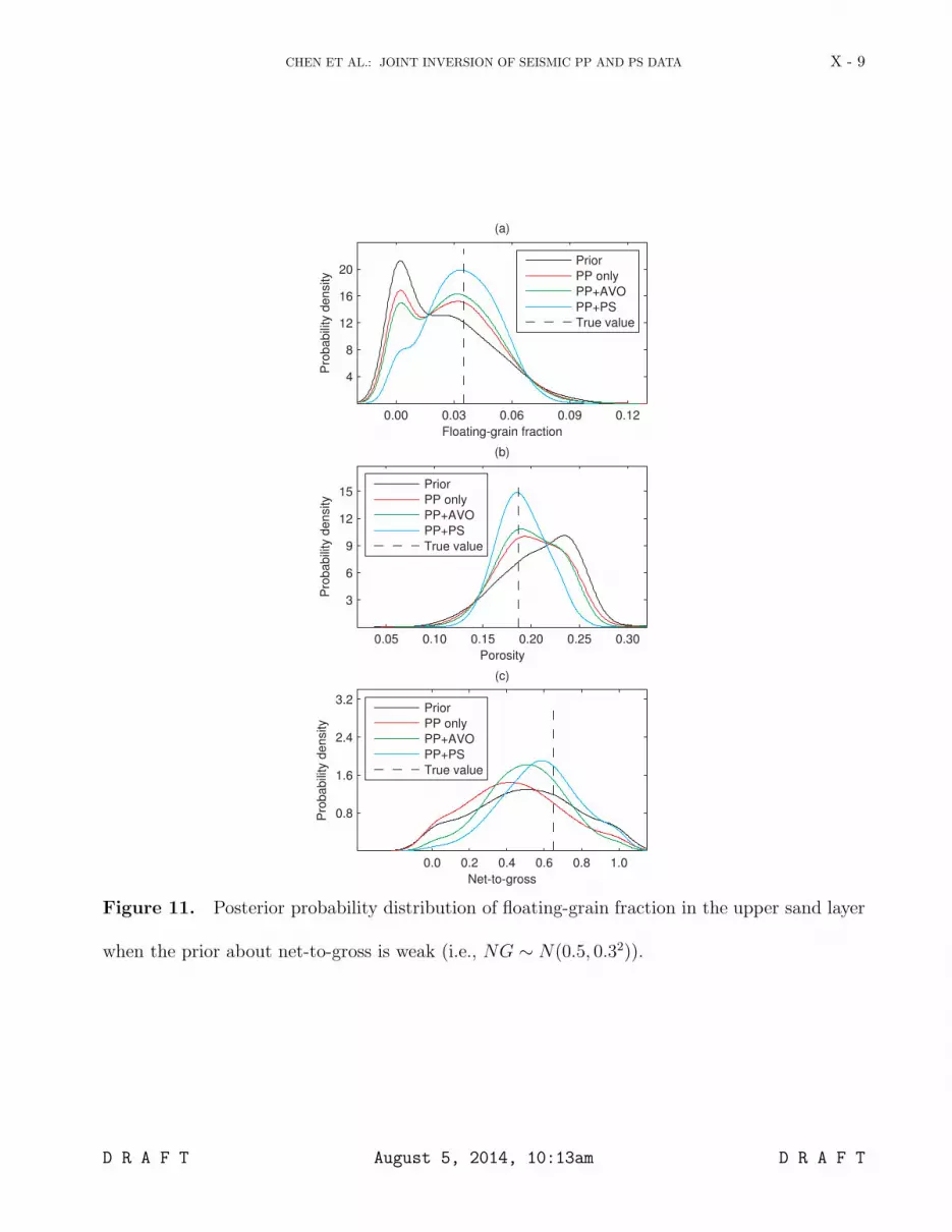
To explore the effects of prior about net-to-gross, we use less informative prior 21

(i.e., 2~ (0.5,0.3 )NG N ) for net-to-gross and good prior about floating-grain fraction (22

2~ (0.02,0.03 )X N ). Since the properties in the lower-pay layer are much less sensitive 23

22

to seismic data, we only do the comparison for the upper-pay layer. Similar to what we 1

found earlier, the combination of PP and PS data significantly improve the estimates of 2

floating-grain fraction and porosity. Unlike the previous comparison in Figures 8c and 9c, 3

we found the combined use of PP and PS data in this case significantly improve the 4

estimates of net-to-gross when it has significant uncertainty (see Figure 11c). 5

In reality, it is more difficult to collect and process PS and AVO gradient data 6

compared to PP data. Therefore, they are likely subject to larger noise. To explore the 7

effects of noise levels on reservoir parameter estimation, we let the prior of floating-grain 8

fraction be 2~ (0.02,0.03 )X N and let net-to-gross prior be 2~ (0.6,0.1 )NG N . We set 9

the noise level in the PP data still as 0.01 RFC but noise levels in the PS and AVO 10

gradient data as 0.02 RFC. Figure 12 shows the posterior PDFs of floating-grain fraction, 11

porosity and net-to-gross. Although the estimated results are slightly worse than those 12

obtained using noise levels of 0.01 RFC for all the seismic data (see Figure 8), the 13

conclusions remain the same. 14

Comparison of discrepancies between the estimated and the true values 15

Since we use sampling-based methods for inversion, we can obtain many samples 16

of other variables as given in equation 20, such as effective P-wave and S-wave velocity, 17

density, layer-thickness, etc. With the use of those samples, we can not only visually 18

compare prior and posterior PDFs but also calculate a wide range of statistics. In the 19

previous comparisons, we qualitatively compare the posterior estimates with their 20

corresponding priors. To demonstrate the value of PS data, in this subsection, we 21

quantitatively compare the estimated results with their corresponding true values. 22

23

We first compare the difference between the estimated median and the true value, 1

which measures how accurate a chosen point estimator (in this case, median) to the true 2

value of a given parameter. Figure 13a compares the differences between the estimated 3

floating-grain fraction, porosity, and net-to-gross values with their true values. The priors 4

for floating-grain fraction is 2~ (0.0,0.05 )X N and for net-to-gross is 2~ (0.6,0.1 )NG N , 5

and the noise levels are 0.01 RFC for PP data and 0.02 for other data sets. We normalize 6

the results by the difference obtained from prior distributions. For net-to-gross, as we 7

demonstrated early, under the good prior, the estimated medians do not improve the prior 8

medians. The value slightly over 1.0 may reflect the effects of noise in seismic data or 9

sampling variations during the inversion procedure. For floating-grain fraction and 10

porosity, when conditioning to PP data, the differences are significantly reduced. When 11

adding AVO gradient data, the improvement is minimal, but adding PS data leads to 12

further reduction. 13

Figure 13b compares the differences for effective P-wave and S-wave velocity, 14

effective density, and layer thickness. For effective P-wave velocity and density, 15

conditioning to PP data significantly improves the accuracy, and further adding AVO 16

gradients or PS data does not lead to a significant reduction. However, for estimation of 17

effective S-wave velocity and layer thickness, either adding AVO gradient stacks or PS 18

data lead to further reduction of the discrepancies, but adding the PS data gives the best 19

results. For density, adding PS data does not lead to significant reduction in uncertainty. 20

This is because for the current case study, after conditioning to PP data, the uncertainty is 21

already very small, leaving less room for further improvement. 22

Comparison of widths of uncertainty bounds 23

24

The MCMC-based methods also allow us to quantitatively compare the uncertainty 1

associated with all the estimation. In this study, we calculate the widths of 95% predictive 2

intervals. Similar to the comparison of the discrepancies, we normalize the results by 3

those obtained from the prior PDFs. 4

Figure 14 shows the results for reservoir parameters and for effective parameters. 5

For reservoir parameters (i.e., floating-grain fraction, porosity, and net-to-gross), the 6

reduction of uncertainty is small and the maximum reduction is around 20%. The use of 7

various combinations of seismic data does not seem to make a significant difference. For 8

P-wave velocity and density, after conditioning to PP data, adding AVO gradient data or 9

PS data does not lead further significant reduction. However, for S-wave velocity and 10

layer thickness, adding PS data causes significantly more reduction in the uncertainty 11

than adding AVO gradient data. 12

Comparison of predictive probabilities 13

In the previous sections, we compare the discrepancies between the estimated and 14

true value and the widths of uncertainty bounds, both of which just compare one aspect of 15

posterior PDFs. A better evaluation is to compare the predictive probabilities of a small 16

interval around the true value, which is given by 17

Prob( [(1 ) ,(1 ) ] | Data)True Trueβ ε β ε β∈ − + . (29) 18

In equation 29, symbol β represents a variable under estimation. We set 2.5%ε = for 19

effective density and 5% for other parameters because the posterior density has much 20

smaller uncertainty compared to other effective properties. The large predictive 21

probability means that the data provide stronger evidence to support the occurrence of the 22

true values. Again, we normalize the probabilities by the prior predictive probability. 23

25

Figure 15a compares the predictive probability ratios of floating-grain fraction, 1

porosity, and net-to-gross. These results are more consistent than those shown in Figures 2

13a and 14a as the ratios of net-to-gross are very close to 1.0. This means that for the 3

tight prior of net-to-gross ( 2~ (0.6,0.1 )NG N ), the updating is ignorable. For floating-4

grain fraction and porosity, the use of PP data significantly increases the predictive 5

probabilities. Adding AVO gradient data does not cause significant improvement. 6

However, adding PS data leads to significant improvement again. Figure 15b shows the 7

comparison for effective P-wave and S-wave velocity, effective density, and layer 8

thickness. Similarly, we found that adding PS data significantly improves the estimates of 9

effective S-wave velocity and layer thickness compared to Figures 14b and 15b. 10

CONCLUSIONS 11

We started from likelihood analysis of a simple two-layer model, with the first 12

layer being shale and the second layer being sand, and found that seismic PS data are 13

significantly more informative than AVO gradient data, even with the high-order term 14

included, for reservoir parameter estimation. Although this analysis is based on a 15

floating-grain rock physics model, it is straightforward to extend the method to other rock 16

physics models. We assume in the study that we have a suitable rock physics model to 17

link seismic attributes to reservoir parameters and seismic data are of reasonable quality. 18

Without those assumptions, we may not be able to verify the benefits of using PS data. 19

We developed a hierarchical Bayesian model to combine PP and PS data for 20

complicated situations (e.g., multiple layers, a large number of unknowns, etc), motivated 21

by the analytical results. We inverted PS data directly in the PS time domain unlike many 22

previous methods, which first convert PS time to PP time and then invert PS data in the 23

26

PP time domain. The alignment of PP and PS time in our model is carried out by 1

identifying one common reflection interface and using the PP and PS time to the common 2

interface as references. This avoids many difficulties caused by the conversion of PS time 3

to PP time, such as the distortion of wavelets, and the requirement of knowing internal P-4

wave to S-wave velocity ratios a-priori. 5

We performed comparison studies based on a synthetic six-layer model to 6

demonstrate the value of PS data for estimating reservoir parameters. PS data are very 7

helpful for improving the estimates of porosity and floating-grain fraction and for 8

improving the estimates of effective S-wave velocity and layer-thickness under a range of 9

priors and noise levels in seismic data. Net-to-gross is relatively less sensitive to PS data. 10

Compared to the posterior results obtained from PP plus AVO gradient data, PP data are 11

most informative for parameter estimation, then PS data, and finally AVO gradient data. 12

This suggests that to improve the estimates of reservoir parameters, PS data are more 13

valuable because PS data can provide complementary information to PP data, and give 14

similar but better information than AVO gradient data. Consequently, they have the 15

potential of significantly improving parameter estimation results. 16

We claim that PS data are more informative than AVO gradient data for reservoir 17

parameter estimation. To be precise, the PS data include some information from the 18

matching between PP and PS time because we considered PS time registration as data in 19

the model. The success of using PS data in the inversion depends on the existence of at 20

least one reference PS time. In the cases where we cannot find a good matching between 21

PP and PS time, we may pick up multiple possible matching with uncertainty. Under 22

these situations, the value of using PS data may be less apparent than what we have 23

27

demonstrated in the six-layer models. In addition, since we used the convolution method 1

for forward simulation of PP and PS responses, we need to have known PP and PS 2

wavelets. This could be difficult in practice and thus limits the applicability of the current 3

model. 4

ACKNOWLEDGMENTS 5

We thank Ion Geophysical for funding and for permission to publish this work. We 6

thank James Gunning from CSIRO for providing help in understanding the Delivery 7

codes and Doug Sassen from Ion Geophysical for helping to answer some questions. We 8

also thank Drs. Sam Kaplan, Helene Hafslund Veire, Miguel Bosch, and one anonymous 9

reviewer for their constructive comments. 10

APPENDIX A 11

DATA MATRICES FOR SYNTHETIC TWO-LAYER MODELS 12

For the case of using only PP data, we set (1,0,0)d =M . For the case of using PP 13

and PS data, we set 14

1 0 00 1 0d⎛ ⎞

= ⎜ ⎟⎝ ⎠

M . (A-1) 15

Similarly, for the case of using PP and AVO gradient traces, we set 16

1 0 00 0 1d⎛ ⎞

= ⎜ ⎟⎝ ⎠

M . (A-2) 17

For the case of using all seismic data, we set 18

28

1 0 00 1 00 0 1

d

⎛ ⎞⎜ ⎟= ⎜ ⎟⎜ ⎟⎝ ⎠

M . (A-3) 1

APPENDIX B 2

DERIVATION OF MEAN VECTOR AND COVARIANCE MATRICES 3

In the current study, we assume that the reservoir parameters under estimation are 4

loading-depth and floating-grain fraction. Let piv , siv , iρ , iz , and ix be seismic P- and S-5

wave velocity, density, loading depth, and floating-grain fraction at the i-th layer, 6

respectively. From the rock physics model in given equation 1-5, we have 7

= .

pi vp vp vp vpi

i si vs vp vs vp vs vp vs vs vp vsi

i vp vp vp vp

ri i i ri

v a b cz

v a a b b b c b bx

a a b b b c b c bρ ρ ρ ρ ρ ρ ρ

εε ε

ρ ε ε

⎛ ⎞ ⎛ ⎞ ⎛ ⎞⎛ ⎞⎛ ⎞⎜ ⎟ ⎜ ⎟ ⎜ ⎟⎜ ⎟= = + + + +⎜ ⎟⎜ ⎟ ⎜ ⎟ ⎜ ⎟⎜ ⎟ ⎝ ⎠⎜ ⎟ ⎜ ⎟ ⎜ ⎟ ⎜ ⎟+ + +⎝ ⎠ ⎝ ⎠ ⎝ ⎠ ⎝ ⎠

+ +

r

µ H α ε (B-1) 8

We can form vectors and matrices for all the layers by stacking those layer-based vectors 9

and matrices, i.e., 1 2( , , , )T T T Tn=r r r rL , 1 2( , , , )T T T T

r n=µ µ µ µL , 1 2( , , , )T T T Tn=α α α αL , 10

1 2( , , , )T T T Tr n=ε ε ε εL , and 1 2( , , , )T T T T

n=H H H HL . 11

It is straightforward to derive the covariance matrix from equation B-1 by assuming 12

that residuals vpε , vsε , and ρε in equations 1-3 have Gaussian distributions with zero 13

mean and variances of 2vpσ , 2

vsσ , and 2ρσ , respectively. Specifically, the matrix is 14

2 2 2 2

2 2 2

1/ .

/

vs

ri vp vs vs vs vp vs

vs vp

b bb b b bb b b b

ρ

ρ

ρ ρ ρ ρ

σ σ σσ σ

⎛ ⎞⎜ ⎟Σ = +⎜ ⎟⎜ ⎟+⎝ ⎠

(B-2) 15

29

The covariance matrix 1 2( , , , ).r ndiagΣ = Σ Σ ΣL 1

2

30

REFERENCES 1

Aki, K., and P. G. Richards, 1980, Quantitative seismology: Theory and methods: W. H. 2

Freeman and Co. 3

Bale, R., T. Marchand, K. Wilkinson, K. Wikel, and R. Kendall, 2013, The signature of 4

shear-wave splitting: Theory and observations on heavy oil data: The Leading Edge, 5

32, 14-24. 6

Bansal, R., and M. Matheney, 2010, Wavelet distortion correction due to domain 7

conversion: Geophysics, 75, No. 6, V77-V87. 8

Bernardo, J. M., and F. M. Smith, 2000, Bayesian theory: John Wiley & Sons, LTD. 9

Brettwood, P., J. P. Leveille, and S. Singleton, 2013, C-wave data improve seismic 10

imaging: The American Oil & Gas Reporter, 1. 11

Castagna, J. P., H. W. Swan, and D. J. Foster, 1998, Framework for AVO gradient and 12

intercept interpretation: Geophysics, 63, No. 3, 948-956. 13

Chen, J., A. Kemna, and S. Hubbard, 2008, A comparison between Gauss-Newton and 14

Markov chain Monte Carlo based methods for inverting spectral induced polarization 15

data for Cole-Cole parameters: Geophysics, 73, No. 6, F247-F259. 16

Davis, T. L., A. Bibolova, S. O’Brien, D. Klepacki, and H. Robinson, 2013, Prediction of 17

residual oil saturation and cap-rock integrity from time-lapse, multicomponent seismic 18

data, Delhi field, Louisiana: The Leading Edge, 32, 26-31. 19

DeMartini, D. C., and M. E. Glinsky, 2006, A model for variation of velocity versus 20

density trends in porous sedimentary rocks: Journal of Applied Physics, 100, 014910. 21

31

Gardner, G. H. F., L. W. Gardner, and A. R. Gregory, 1974, Formation velocity and 1

density – The diagnostic basics for stratigraphic traps: Geophysics, 39, No. 6, 770-2

780. 3

Glinsky, M. E., A. Cortis, D. Sassen, H. Rael, and J. Chen, 2013, Rock physics and 4

geophysics for unconventional resources, multicomponent seismic, quantitative 5

interpretation: The 2nd International Workshop on Rock Physics (2IWRP), 2013, South 6

Hampton, United Kingdom, August 4-9, http://arxiv.org/abs/1304.6048. 7

Gunning, J., and M. E. Glinsky, 2004, Delivery: an open-source model-based Bayesian 8

seismic inversion program: Computers and Geosciences, 30, 619-636. 9

Gunning, J., and M. E. Glinsky, 2007, Detection of reservoir quality using Bayesian 10

seismic inversion: Geophysics, 72, No. 3, R37-R49. 11

Hardage, B. A., M. V. DeAngelo, P. E. Murray, and D. Sava, 2011, Multicomponent 12

seismic technology: Society of Exploration Geophysicists. 13

Mahmoudian, F., and G. F. Margrave, 2004, Three-parameter AVO inversion with PP 14

and PS data using offset-binning: CREWES Report, 16. 15

Pacal, E. E., 2012, Seismic imaging with ocean-bottom nodes (OBNs): new acquisition 16

designs and the Atlantis 4C OBN: Master Thesis, University of Houston. 17

Rodriguez-Saurez, C., 2000, Advanced marine methods: ocean- bottom and vertical cable 18

analyses: PhD Thesis, University of Calgary. 19

Stewart, R. R., J. E. Gaiser, R. J. Brown, and D. C. Lawton, 2002, Tutorial: Converted-20

wave seismic exploration: methods: Geophysics, 67, No. 5, 1348-1363. 21

32

Stone, C. J., 1995, A course in probability and statistics: Duxbury Press. 1

Tarantola, A., 2005, Inverse problem theory and methods for model parameter 2

estimation: The Society for Industrial and applied mathematics (SIAM), Philadelphia, 3

PA. 4

Veire, H. H., and Landrø, M., 2006, Simultaneous inversion of PP and PS seismic data: 5

Geophysics, 71, No. 3, R1–R10. 6

Venables, W. N., and B. D. Ripley, 1999, Modern applied statistics with S-Plus, Third 7

Edition, Springer, New York. 8

9

33

FIGURE CAPTIONS 1

Figure 1: Likelihoods of floating-grain fraction given various data combinations for the 2

true value of (a) 0.0%, and (b) 3.5%. 3

Figure 2: Likelihood ratios of using various combinations of seismic data compared to 4

that of using PP data only as a function of measurement errors in PS and AVO 5

gradient data for the true value of (a) 0.0%, and (b) 3.5%. 6

Figure 3: Dependent relationships among unknown parameters and data. 7

Figure 4: Various logs from an actual borehole as a function of depth: (a) P-wave 8

velocity (km/s), (b) S-wave velocity (km/s), (c) density (g/cc), (d) Vp/Vs, and (e) P-9

Impedance (MPa). 10

Figure 5: Blocked values obtained from the borehole logs using Backus average as a 11

function of relative depth: (a) P-wave velocity (km/s), (b) S-wave velocity (km/s), (c) 12

density (g/cc), (d) Vp/Vs, and (e) P-Impedance (MPa). 13

Figure 6: Synthetic seismic PP (a) and PS (b) data as a function of P-wave incident 14

angles. 15

Figure 7: Selected realizations of effective P-wave (a) and S-wave (b) velocity and 16

density (c) using a thinning of 50 from the 10,000 samples, where the red line 17

segments are the true values. 18

Figure 8: Posterior probability distributions of floating-grain fraction (a), porosity (b), 19

and net-to-gross (c) in the upper sand layer when priors about floating-grain fraction 20

34

and net-to-gross are strong (i.e., 2(0.02, 0.03 )X N: , and 2(0.6, 0.1 )NG N: , the 1

reference case). 2


and net-to-gross (c) in the upper sand layer when the prior about floating-grain 4

fraction is weak (i.e., 2(0.0, 0.05 )X N: ). 5


and net-to-gross (c) in the lower sand layer when priors about floating-grain fraction 7

and net-to-gross are strong (i.e., 2(0.02, 0.03 )X N: , and 2(0.6, 0.1 )NG N: ). 8


and net-to-gross (c) in the upper sand layer when the prior about net-to-gross is weak 10

(i.e., 2(0.5, 0.3 )NG N: ). 11


and net-to-gross (c) in the upper sand layer when the errors in the AVO gradient and 13

PS data are doubled. 14

Figure 13: Comparison of differences between the true values and estimated medians for 15

priors 2(0.0, 0.05 )X N: , 2(0.6, 0.1 )NG N: , and noise of 0.01 RFC for PP data and 16

0.02 RFC for others, where 'R0' represents PP data only, 'R0R1' represents PP plus PS 17

data, 'R0R2' represents PP plus AVO gradient data, and 'R0R1R2' represents all the 18

data. 19

Figure 14: Comparison of half-widths of 95% predictive intervals for priors 20

2(0.0, 0.05 )X N: , 2(0.6, 0.1 )NG N: , and noise of 0.01 RFC for PP data and 0.02 21

35

RFC for others, where 'R0' represents PP data only, 'R0R1' represents PP plus PS data, 1

'R0R2' represents PP plus AVO gradient data, and 'R0R1R2' represents all the data. 2

Figure 15: Comparison of predictive probability of the true values for priors 3

2(0.0, 0.05 )X N: , 2(0.6, 0.1 )NG N: , and noise of 0.01 RFC for PP data and 0.02 4

RFC for others, where 'R0' represents PP data only, 'R0R1' represents PP plus PS data, 5

'R0R2' represents PP plus AVO gradient data, and 'R0R1R2' represents all the data. 6

Table 1: Sand and shale rock-physics model coefficients from actual borehole logs

Regression Equations Standard Errors Units

Sand

645 0.508 5490pv z x= + + 105 m/s

1220 0.894s pv v= − + 69 m/s

41.70 1.65 10 1.56pv xρ −= + × + 0.0149 g/cc

Shale

1640 0.946pv z= − + 145 m/s

1030 0.801s pv v= − + 63 m/s

0.1660.651 pvρ = 0.030 g/cc

CHEN ET AL.: JOINT INVERSION OF SEISMIC PP AND PS DATA X - 1

0.03 0.06 0.09 0.12 0.15 0.18

3

6

9

12

15

Floating-grain fraction

Lik

elih

ood

(a)

PP only

PP+AVO

PP+PS

All data

0.03 0.06 0.09 0.12 0.15 0.18

2

4

6

8

10


Lik

elih

ood

(b)

PP only

PP+AVO

PP+PS

All data

Figure 1. Likelihoods of floating-grain fraction given various data combinations for the true

value of (a) 0.0% and (b) 3.5%.

D R A F T August 5, 2014, 10:13am D R A F T

X - 2 CHEN ET AL.: JOINT INVERSION OF SEISMIC PP AND PS DATA

0.02 0.04 0.06 0.08 0.10

1.1

1.2

1.3

1.4

1.5

Noise level (RFC)

Lik

elih

ood r

atio

(a)

PP+AVO vs. PP

PP+PS vs. PP

All data vs. PP

0.02 0.04 0.06 0.08 0.10

1.1

1.2

1.3

1.4

1.5

Noise level (RFC)

Lik

elih

ood r

atio

(b)

PP+AVO vs. PP

PP+PS vs. PP

All data vs. PP

Figure 2. Likelihood ratios of using various combinations of seismic data compared to that of

using PP data only as a function of measurement errors in PS and AVO gradient data.

Figure 3. Dependent relationships among unknown parameters and data.



3 4 5

2.52

2.56

2.60

2.64

(a)

Vp (km/s)

Depth

TV

D (

×10

4)

1 2 3

2.52

2.56

2.60

2.64

(b)

Vs (km/s)

2.3 2.5 2.7

2.52

2.56

2.60

2.64

(c)

Density (g/cc)

1.6 2.0 2.4

2.52

2.56

2.60

2.64

(d)

Vp/Vs

6 10 14

2.52

2.56

2.60

2.64

(e)

Zp (MPa)

Figure 4. Various logs from an actual borehole as a function of depth: (a) P-wave velocity

(km/s), (b) S-wave velocity (km/s), (c) density (g/cc), (d) Vp/Vs, and (e) P-Impedance (MPa).



2.8 3.2 3.6

0.2

0.4

0.6

0.8

1.0

(a)

Vp (km/s)

Norm

aliz

ed d

epth

1.2 1.6 2.0

0.2

0.4

0.6

0.8

1.0

(b)

Vs (km/s)

2.3 2.4 2.5

0.2

0.4

0.6

0.8

1.0

(c)

Density (g/cc)

2.0 2.2 2.4

0.2

0.4

0.6

0.8

1.0

(d)

Vp/Vs

7.0 8.0 9.0

0.2

0.4

0.6

0.8

1.0

(e)

Zp (MPa)

Figure 5. Blocked values obtained from the borehole logs using Backus average as a function

of relative depth: (a) P-wave velocity (km/s), (b) S-wave velocity (km/s), (c) density (g/cc), (d)

Vp/Vs, and (e) P-Impedance (MPa).

9 27 45

7.35

7.45

7.55

7.65

Angle (degrees)

Tim

e (

ms)

(a)

9 27 45

8.90

9.00

9.10

9.20

9.30

Angle (degrees)

Tim

e (

ms)

(b)

Figure 6. Synthetic seismic PP (a) and PS (b) data as a function of P-wave incident angles.



3.0 3.5 4.0

0.2

0.4

0.6

0.8

1.0

(a)

Vp (km/s)

Norm

aliz

ed d

epth

1.2 1.6 2.0

0.2

0.4

0.6

0.8

1.0

(b)

Vs (km/s)

Norm

aliz

ed d

epth

2.2 2.4 2.6

0.2

0.4

0.6

0.8

1.0

(c)

Density (g/cc)

Norm

aliz

ed d

epth

Figure 7. Selected realizations of effective P-wave (a) and S-wave (b) velocity and density (c)

using a thinning of 50 from the 10,000 samples, where the red line segments are the true values.



0.00 0.03 0.06 0.09 0.12

4

8

12

16

20


Pro

babili

ty d

ensity

(a)

Prior

PP only

PP+AVO

PP+PS

True value

0.05 0.10 0.15 0.20 0.25 0.30

3

6

9

12

15

Porosity

Pro

babili

ty d

ensity

(b)

Prior

PP only

PP+AVO

PP+PS

True value

0.2 0.4 0.6 0.8 1.0

1

2

3

4

5

Net-to-gross

Pro

babili

ty d

ensity

(c)

Prior

PP only

PP+AVO

PP+PS

True value

Figure 8. Posterior probability distribution of floating-grain fraction in the upper sand layer

when priors about floating-grain fraction and net-to-gross are strong (i.e., X ∼ N(0.02, 0.032),

and NG ∼ N(0.6, 0.12), the reference case).



0.00 0.03 0.06 0.09 0.12

5

10

15

20

25

30


Pro

babili

ty d

ensity

(a)

Prior

PP only

PP+AVO

PP+PS

True value

0.05 0.10 0.15 0.20 0.25 0.30

3

6

9

12

15

Porosity

Pro

babili

ty d

ensity

(b)

Prior

PP only

PP+AVO

PP+PS

True value

0.2 0.4 0.6 0.8 1.0

1

2

3

4

5

Net-to-gross

Pro

babili

ty d

ensity

(c)

Prior

PP only

PP+AVO

PP+PS

True value


when the prior about floating-grain fraction is weak (i.e., X ∼ N(0.0, 0.052)).



0.00 0.03 0.06 0.09 0.12

4

8

12

16

20


Pro

babili

ty d

ensity

(a)

Prior

PP only

PP+AVO

PP+PS

True value

0.05 0.10 0.15 0.20 0.25 0.30

3

6

9

12

15

Porosity

Pro

babili

ty d

ensity

(b)

Prior

PP only

PP+AVO

PP+PS

True value

0.2 0.4 0.6 0.8 1.0

1

2

3

4

5

Net-to-gross

Pro

babili

ty d

ensity

(c)

Prior

PP only

PP+AVO

PP+PS

True value

Figure 10. Posterior probability distribution of floating-grain fraction in the lower sand layer

when priors about floating-grain fraction and net-to-gross are strong (i.e., X ∼ N(0.02, 0.032),

and NG ∼ N(0.6, 0.12)).



0.00 0.03 0.06 0.09 0.12

4

8

12

16

20


Pro

babili

ty d

ensity

(a)

Prior

PP only

PP+AVO

PP+PS

True value

0.05 0.10 0.15 0.20 0.25 0.30

3

6

9

12

15

Porosity

Pro

babili

ty d

ensity

(b)

Prior

PP only

PP+AVO

PP+PS

True value

0.0 0.2 0.4 0.6 0.8 1.0

0.8

1.6

2.4

3.2

Net-to-gross

Pro

babili

ty d

ensity

(c)

Prior

PP only

PP+AVO

PP+PS

True value


when the prior about net-to-gross is weak (i.e., NG ∼ N(0.5, 0.32)).



0.00 0.03 0.06 0.09 0.12

5

10

15

20

25

30


Pro

babili

ty d

ensity

(a)

Prior

PP only

PP+AVO

PP+PS

True value

0.05 0.10 0.15 0.20 0.25 0.30

3

6

9

12

15

Porosity

Pro

babili

ty d

ensity

(b)

Prior

PP only

PP+AVO

PP+PS

True value

0.2 0.4 0.6 0.8 1.0

1

2

3

4

5

Net-to-gross

Pro

babili

ty d

ensity

(c)

Prior

PP only

PP+AVO

PP+PS

True value


when the errors in the AVO gradient and PS data are doubled.



Prior R0 R0R2 R0R1 R0R1R2

0.5

1.0

1.5

Used data

Norm

aliz

ed d

iffe

rence

(a)

Floating−grain fraction

Porosity

Net−to−gross


0.5

1.0

1.5

Used data

Norm

aliz

ed d

iffe

rence

(b)

Effective vp

Effective vs

Effective density

Thickness

Figure 13. Comparison of differences between the true values and estimated medians for

priors X ∼ N(0.0, 0.052), NG ∼ N(0.6, 0.12), and noise of 0.01 RFC for PP data and 0.02

RFC for others, where ’R0’ represents PP data only, ’R0R1’ represents PP plus PS data, ’R0R2’

represents PP plus AVO gradient data, and ’R0R1R2’ represents all the data.




0.3

0.6

0.9

1.2

1.5

Used data

Wid

th o

f 95%

inte

rvals

(a)


Porosity

Net−to−gross


0.3

0.6

0.9

1.2

1.5

Used data

Wid

th o

f 95%

inte

rvals

(b)

Effective vp

Effective vs

Effective density

Thickness

Figure 14. Comparison of half-widths of 95% predictive intervals for priors X ∼ N(0.0, 0.052),

NG ∼ N(0.6, 0.12), and noise of 0.01 RFC for PP data and 0.02 RFC for others, where ’R0’

represents PP data only, ’R0R1’ represents PP plus PS data, ’R0R2’ represents PP plus AVO

gradient data, and ’R0R1R2’ represents all the data.




1.0

1.5

2.0

2.5

3.0

Used data

Pro

babili

ty r

atio

(a)


Porosity

Net−to−gross


1.0

1.5

2.0

2.5

3.0

Used data

Pro

babili

ty r

atio

(b)

Effective vp

Effective vs

Effective density

Thickness

Figure 15. Comparison of predictive probability of the true values for priorsX ∼ N(0.0, 0.052),

NG ∼ N(0.6, 0.12), and noise of 0.01 RFC for PP data and 0.02 RFC for others, where ’R0’

represents PP data only, ’R0R1’ represents PP plus PS data, ’R0R2’ represents PP plus AVO

gradient data, and ’R0R1R2’ represents all the data.


Documents

Stochastic inversion of seismic PP and PS data for reservoir parameter estimation