Stress Resultant Based Elasto-Viscoplastic Thick Shell Model

Shock and Vibration 19 (2012) 477–492 477DOI 10.3233/SAV-2011-0644IOS Press

Stress resultant based elasto-viscoplastic thickshell model

Pawel Woelke∗, Ka-Kin Chan, Raymond Daddazio and Najib AbboudWeidlinger Associates, New York, NY, USA

Received 24 April 2010

Revised 4 June 2011

Abstract. The current paper presents enhancement introduced to the elasto-viscoplastic shell formulation, which serves as atheoretical base for the finite element code EPSA (Elasto-Plastic Shell Analysis) [1–3]. The shell equations used in EPSA aremodified to account for transverse shear deformation, which is important in the analysis of thick plates and shells, as well ascomposite laminates. Transverse shear forces calculated from transverse shear strains are introduced into a rate-dependent yieldfunction, which is similar to Iliushin’s yield surface expressed in terms of stress resultants and stress couples [12]. The hardeningrule defined by Bieniek and Funaro [4], which allows for representation of the Bauschinger effect on a moment-curvature plane,was previously adopted in EPSA and is used here in the same form. Viscoplastic strain rates are calculated, taking into accountthe transverse shears. Only non-layered shells are considered in this work.

Keywords: Thick plates and shells, transverse shear deformation, elasto-viscoplastic analysis, rate dependent response

1. Introduction

Our objective is to introduce transverse shear strains and forces into the elasto-viscoplastic model of shell behavior,formulated within the finite element code EPSA. Only matters directly related to this objective are discussed indetail. For details of the finite element formulation, the reader is directed to references [1–4,8].

In our formulation, we use the following hypothesis: plane sections originally perpendicular to the middle surfaceremain plane after deformation but not perpendicular to the middle surface (Fig. 1). From this hypothesis, we deducethat bending displacements u and v along x and y directions are:

u = zφx and v = −zφy (1)

where φx and φy are the angles of rotation of the sections originally perpendicular to the middle section in the xzand yz planes, respectively, expressed by:

φx = −∂w

∂x+ γxz and φy =

∂w

∂y− γyz (2)

where w is the vertical displacement in the z direction and γxz, γyz are the transverse shear strains in the xz and yzplanes, respectively.

Shells in which the ratio of the thickness to the radius of curvature is equal to or less than 1/50 are often consideredthin (both lower and higher ratios are often used as an indication of shell thickness). In the case of thin shells,transverse shear strains are negligible. This is true for most boundary conditions. Some types of loading conditions,however, cause significant shear forces, regardless of the thickness of the structure. An example of such a loadingcondition is a concentrated bending moment applied at mid-span of the beam, plate, or shell (Fig. 2).

∗Corresponding author. Tel.: +1 212 367 2983, ext: 3000; Fax: +1 212 497 2483; E-mail: [email protected]; [email protected].

ISSN 1070-9622/12/$27.50 2012 – IOS Press and the authors. All rights reserved

AUTH

OR

COPY

478 P. Woelke et al. / Stress resultant based elasto-viscoplastic thick shell model

Fig. 1. Transverse shear deformations [24].

Fig. 2. Concentrated couples formed by: a) the vertical forces causing significant shear forces, and b) the horizontal forces – no significant shearforces [10].

The concentrated bending moment can be applied in two ways – by the vertical force couple (Fig. 2a) or by thehorizontal force couple (Fig. 2b). With the former, a large shear force is generated at mid-span of the beam. Theforce increases as the distance between the forces s decreases. To correctly represent the beam deformation in thiscase, it is necessary to consider transverse shear strains, regardless of the beam thickness. The same situation occurswhen such loading conditions are applied to plates and shells.

Transverse shear strains and forces are especially important in the analysis of composite laminates. Shearcontributes significantly to delamination, a common failure mode in composites. In the current paper, only isotropicplates and shells are considered.

An Iliushin’s yield function [12] modified to account for transverse shear forces, as well as the Bauschinger effect,is adopted. Transverse shear forces are known to significantly affect the plastic behavior of both thick and, undercertain loading conditions, thin shells. Thus, shear forces are introduced into the yield function, in accordance withShapiro’s approach [20].

In the elasto-viscoplastic calculations, we follow the approach of Perzyna, who proposed a set of constitutiveequations representing viscoplastic strain hardening for arbitrary loading histories [16]. The viscoplastic strainrate vector is directed along the normal to the subsequent dynamic yield surface. The quasi-static yield surfaceis defined in the stress resultant space (non-layered method), following an approach proposed by Iliushin [12].Bieniek and Funaro [4] introduced hardening parameters into Iliushin’s yield function in the form of residualbending moments, allowing for description of the Bauschinger effect on the moment-curvature plane. Voyiadjis and

AUTH

OR

COPY

P. Woelke et al. / Stress resultant based elasto-viscoplastic thick shell model 479

Woelke [24] extended this idea, defining a three-dimensional kinematic hardening rule that uses not only residualbending moments, but residual normal and shear forces. We use Bieniek’s and Funaro’s definition of hardeningparameters [4]. We modify the quasi-static yield surface to account for shear forces, as in Shapiro’s approach [20].

Numerical integration of stresses through the thickness is not necessary with the non-layered formulation, makingit less expensive computationally. Although the approximation of the yield criterion expressed in terms of forcesand moments was expected to result in a loss of accuracy, this turned out not to be the case, as demonstrated bymany authors who compared the two methods [1,21,24].

This paper is organized into six sections. Following the Introduction, Section 2 discusses the shell constitutiveequations. Section 3 describes the finite element procedure. Section 4 defines the dynamic and quasi-static yieldsurface, flow, and hardening rules. Section 5 offers numerical examples, confirming that the current formulationprovides good approximations. Section 6 presents the conclusion.

2. Shell constitutive equations

The plate or shell is assumed to be a solid, single-layer surface with thickness h (Fig. 1). The basic assumptionsof the shell formulation are similar to those of Bieniek and Funaro [4]. At any point of the shell, the membranestrains and curvatures in a rectangular coordinate system (x, y, z) are expressed by the following equations:

ex =∂u0

∂x(3)

ey =∂v0

∂y(4)

exy =12

(∂u0

∂y+

∂v0

∂x

)(5)

κx =∂φx

∂x=

∂

∂x

(−∂w

∂x+ γxz

)(6)

κy =∂φy

∂y=

∂

∂y

(∂w

∂y− γyz

)(7)

κxy =12

(∂φx

∂y+

∂φy

∂x

)(8)

The transverse shear strains are calculated using the following equations:

γxz =∂w

∂x+ φx (9)

γyz =∂w

∂y− φy (10)

In Eqs (3)–(10) z is a measure of the distance between the middle surface of the shell and the surface underconsideration (Fig. 1); ex, ey are membrane strains; exy is in-plane shear strain; κx, κy, κxy are curvatures at themid-surface in planes parallel to the xz, yz, and xy planes, respectively; u, v, w are the displacements along thex, y, z axes, respectively (Figs 1, 2); γxz, γyz are transverse shear strains in xz and yz planes (Fig. 1); and φx, φy

are angles of rotation of the cross-sections normal to the mid-surface of the undeformed shell (Fig. 1).The total normal strains due to both membrane and bending deformation in x, y directions, respectively, can be

expressed as:

εx = ex + zκx and εy = ey + zκy (11)

AUTH

OR

COPY

https://www.researchgate.net/publication/245058617_General_non-linear_finite_element_analysis_of_thick_plates_and_shells?el=1_x_8&enrichId=rgreq-a997a9ab-c618-475c-8241-32846e070848&enrichSource=Y292ZXJQYWdlOzI2MzI3ODk3ODtBUzoxMTA5MTUyMzYxNDMxMDRAMTQwMzQ1NTY2MTg4NA==

https://www.researchgate.net/publication/245058617_General_non-linear_finite_element_analysis_of_thick_plates_and_shells?el=1_x_8&enrichId=rgreq-a997a9ab-c618-475c-8241-32846e070848&enrichSource=Y292ZXJQYWdlOzI2MzI3ODk3ODtBUzoxMTA5MTUyMzYxNDMxMDRAMTQwMzQ1NTY2MTg4NA==


Fig. 3. Stress resultants on plate/shell element.

The stress resultants and couples Mx, My, Mxy, Nx, Ny, Nxy, Qx, Qy shown in Fig. 3 can be expressed in termsof the strains given above:

Mx = D [κx + νκy] (12)

My = D [κy + νκx] (13)

Mxy = D (1 − ν)κxy (14)

Nx = S [ex + νey] (15)

Ny = S [ey + νex] (16)

Nxy = S (1 − ν) exy (17)

Qx = Tγxz (18)

Qy = Tγyz (19)

where:

D =Eh3

12 (1 − ν2), S =

Eh

(1 − ν2), T =

512

Eh

(1 + ν)(20)

and E is Young’s Modulus, h is the shell thickness, and ν is Poisson’s ratio. The positive directions of the stressresultants given by Eq (12)–(19) are shown in Fig. 3:

The above constitutive equations are universal for both plates and shells. The shell curvature is modeled throughfinite element discretization. When shear deformation is neglected, the constitutive Eqs (12)–(19) reduce to thosegiven by Flugge [9].

3. Finite element formulation

The current element is a flat, constant-strain shell element with 4 nodes and 5 degrees of freedom per node,i.e., linear velocities u, v, w in x, y, z directions, respectively, and angular velocities φx, φy around y and x axes,respectively. The positive directions of the degrees of freedom are the same as the positive directions of the stressresultants (Fig. 3).

Details of the kinematics of the element, solution of the equations of motion, time integration scheme, andanti-hourglassing procedure are available in references [1–4,8].

AUTH

OR

COPY


4. Rate-dependent yield function, flow, and hardening rules

As stated in the Introduction,we use a quasi-static yield criterion expressed in terms of stress resultants and couples,proposed by Iliushin [12] and modified by Bieniek and Funaro [4]. The following non-dimensional stress-resultantintensities are defined (Ref. [2,23–25]):

IN =1

N20

(N2

x + N2y − NxNy + 3N2

xy

)(21)

IM =1

M20

(M2

x + M2y − MxMy + 3M2

xy

)(22)

INM =1

N0M0

(NxMx + NyMy − 1

2NxMy − 1

2NyMx + 3NxyMxy

)(23)

IM∗ =1

M20

[(Mx − M∗

x)2 +(My − M∗

y

)2 − (Mx − M∗x)

(My − M∗

y

)+ 3

(Mxy − M∗

xy

)2]

(24)

N0 = σ0h and M0 =σ0h

2

6(25)

σ0 is the static one-dimensional yield strength and h is the shell thickness; M∗ in Eq. (24) are hardening parametersto be defined.

The quasi-static yield surface is [2]:

F (σ) = IN + I2N − I3

N + IM∗ + 0.6 |INM | (26)

Equation (26) describes the current yield surface as the loading path moves from the initial yield surface F0 (σ)toward a limit surface FL (σ). The initial yield surface represents the onset of yielding in the outer shell fibers andis expressed as:

F0 (σ) = IN + IM + 2 |INM | (27)

Time histories of vertical displacement (units – [in]) at point A due to triangular pulse load – with and without sheareffects considered.

The limit yield surface represents the fully plastic cross section and is expressed as:

FL (σ) = 2IN − I2N +

49IM (28)

The hardening parameters M∗ in equation (24) are now defined as [24]:

if F = 1 and ∂F∂σ dσ > 0

dM∗x = B1 (1 − FL) M0

κ0dκx

dM∗y = B1 (1 − FL) M0

κ0dκy

dM∗xy = B2 (1 − FL) M0

κ0dκxy

if F � 1 or ∂F∂σ dσ � 0 then dM∗

x = dM∗y = dM∗

xy = 0

(29)

where κ0 = M0/EI and E is Young’s modulus, I is a second moment of area of the cross-section, and B1 = 9/5and B2 = 4/5. These constants (B1, B2) were determined by comparison with the results obtained with thethrough-the-thickness integration technique described in Ref. [3].

Following the work of Shapiro [20], we account for the influence of shear forces on the plastic behavior of platesand shells. We can include transverse shear forces Qx, Qy by modifying one of the stress intensities, expressed byEq. (21):

IN =1

N20

[N2

x + N2y − NxNy + 3

(N2

xy + Q2x + Q2

y

)](30)

AUTH

OR

COPY


The strain, stress resultants and hardening parameters (residual bending moments) are represented by 8x1 columnmatrices:

eT = {ex, ey, exy, κx, κy, κxy, exz, eyz}sT = {Nx, Ny, Nxy, Mx, My, Mxy, Qx, Qy} (s∗)T = {0, 0, 0, 0, 0, M∗

11, M∗22, M

∗12} (31)

Similarly, ∂F/∂s is expressed as:(

∂F

∂s

)T

={

∂F

∂Nx,

∂F

∂Ny,

∂F

∂Nxy,

∂F

∂Mx,

∂F

∂My,

∂F

∂Mxy,

∂F

∂Qx,

∂F

∂Qy

}(32)

We assume additive decomposition of the strain tensor into elastic and viscoplastic parts:

e = ee + evp (33)

Following Perzyna’s approach [16], Atkatsh et al. developed a generalization of the static yield surface to account forthe strain-rate effects [2–4]. The viscoplastic strain rate tensor is assumed to depend on the stress resultant intensitythrough the associated flow rule:

devp = γRKφ [F (s)]∂F (s)

∂s= λ

∂F (s)∂s

(34)

where K is a work-hardening parameter describing deformation of the quasi-static yield surface during ineleasticprocesses [2–4] and γR and φ (F ) are material response functions (γR is often taken as an inverse of viscositydetermined for a given material). φ (F ) is a Perzyna-type function defined as:

φ (F ) ={

0 for F � 0φ(F ) for F > 0 (35)

By assuming that φ (F ) = F and limiting Eq. (34) to a one-dimensional case, we can express the viscoplastic strainrate as:

devp =2√3γR F

(√F + 1

)(36)

Using Eq. (29), the increment of hardening parameters (residual bending moments) can be written as:

ds∗ = Adλ∂F

∂s′where A = β

Mo

κoand s′ = {0, 0, 0, 0, 0, M11, M22, M12} (37)

Applying the following elastic law:

s = E (e− evp) (38)

and Eq. (34), we can express the viscoplastic multiplier λ as:

λ =

(∂F∂s

)TEde(

∂F∂s

)TE∂F

∂s − (∂F∂s∗

)TA ∂F

∂s′

(39)

where Δt is a time increment, se is the elastic stress vector, and E is the elastic shell stiffness matrix defined byEqs (12)–(20). Because Eq. (39) cannot be solved directly for λ, we solve the equivalent form:

λ =[γR, Δt, K, E, F

[(Se)T

],

∂F

∂S

]= 0 (40)

using an iterative modified falsi method [1–4].Functions γR and φ (F ) can be selected to fit experimental test results of the dynamic behavior of a particular

material. Available experimental methods include a one-dimensional stress-strain test using a Hopkinson bartechnique [14]. γR should be calibrated to adequately represent the results of a multiaxial test on plate and shellspecimens. The experiments should consist of biaxial bending and stretching tests conducted at various loadingrates. The current lack of experimental data precludes choosing function γR to fit measured results. Thus, γR

AUTH

OR

COPY


was selected such that the stress resultants correspond to those obtained using a layered (through-the-thicknessintegration) method [1–4].

For mild steel [7] the proposed function γR takes the form [1–4]:

γR =a1

Fn1 (FL − F )n2 (41)

where F and FL are for one-dimensional cases as in [1–4]:

F =(

σ

σ0

)2

− 1 ; FL =(

σLIM

σ0

)2

− 1 (42)

Material constants a1, n1, n2 were determined for mild steel:

a1 = 30.0; n1 = 0.75; n2 = 0.25 (43)

5. Numerical examples

The reliability of these concepts is verified through a set of discriminating examples. The problems are selected tochallenge new features introduced into the finite element code EPSA, i.e., representation of shear deformation andshear forces in the elasto-viscoplastic shell model. The importance of shear deformation in the analysis of thick shellsis widely known and has been discussed by many authors. The reliability of rate-dependent formulation has alsobeen confirmed [1–4]. The objective of this section is to confirm that the description of shear effects presented hereis reliable and capable of correctly modeling elasto-viscoplastic behavior of thick plates and shells. Both beam andshell problems, simulated with shell elements are used to show the reliability of presented formulation. Although thecurrent work discusses shell element formulation, beams problems (modeled with shell elements) are convenient forverification, since the analytical solutions which serve as references, can be easily established. We note that despitethe geometric simplicity of the beam examples, the boundary conditions are chosen such that the problems presentchallenging tests for accuracy of the new features of the presented shell formulation, i.e. representation of the sheardeformation. The last example considers a cylindrical shell with varying thickness, which allows for investigationof the increasing importance of the shear deformation with increasing thickness of the shell.

5.1. Simply supported beam subjected to a force couple at mid-span

We consider here the simply supported beam discussed in the Introduction. The geometry of the beam, as well asthe shear forces and bending moment diagrams, are given in Fig. 8.

The length of the beam is L = 10 in, the distance between the forces s = 0.625 in, P = 100 lb, M = 62.5 lb in,Young’s modulus is E = 3.0 × 107 psi, and the cross section of the beam is rectangular with b = h = 1.0 in. Theflexural and shear rigidities of the beam are obtained by Eq. (20) with ν = 0, D = 25 × 105 lb in2, and T = 125 ×105 lb.

As noted in the Introduction, there is a significant difference between applications of the concentrated bendingmoment formed by a vertical force couple and those formed by a horizontal one. When distance s is very small,the bending moment diagrams in (Figs 8a and 8b) are almost identical, but the shear force diagrams are different.For the example in (Fig. 8a), there is a very large shear force between points A and B. If the classical (thinshell) formulation is applied, the difference in shear force is immaterial [10]. In reality, however, the shear forcecauses additional strains in the beam, which lead to increased vertical displacement, as well as discontinuity of thedisplacement function between pointsA and B. Only the thick shell formulation, which takes into account transverseshear deformation, is capable of correctly predicting shear effects and vertical displacements in points A and B.

We will confirm that the current formulation features reliable representation of shear effects and is thereforeapplicable to the analysis of thick shells. First we analytically calculate vertical displacement at point A for bothloading cases in (Fig. 4a and 4b), considering the influence of bendingmoments and shear forces (thick beam theory).We will refer to the boundary conditions in Fig. 4 a) as “case a” and Fig. 4 b) as “case b.” We apply the virtual unitforce at pointA, as shown in Fig. 7, to determine the displacement by means of the virtual work principle.

AUTH

OR

COPY


Fig. 4. Simply supported beam subjected to concentrated couples formed by, a) the vertical forces causing significant shear deformation, and b)the horizontal forces – no significant shear deformation [10].

Fig. 5. Simply supported beam subjected to a virtual displacement unit force at point A, virtual bending moment M , and shear force Q diagram.

The vertical displacement at point A, due to bending moment and shear force, is expressed by:

w = wM + wQ =∫L

MM

Ddx +

∫L

QQ

Tdx (44)

where wM and wQ are vertical displacements at point A due to bending moments and shear forces, respectively; Mand Q are virtual bending moment and shear force, as shown in Fig. 7; and M and Q are real bending moment andshear force in the beam.

The integral in Eq. (44) can be calculated using Simpson’s rule or the Mohr-Wereszczegin method. For “case b”the vertical displacement wb = wb

M + wbQ at point A is obtained by:

wb = wbM + wb

Q =14.74

D+

0.0T

= 5.896 × 10−6 in (45)

It is important to note that for “case b” the influence of shear forces is 0. This means that the thin shell formulation,which does not account for transverse shear deformation, produces accurate solutions for the displacement of thebeam only for “case b.”

The vertical displacement for “case a” is:

wa = waM + wa

Q =14.29

D+

29.297T

= 8.056 × 10−6 in (46)

AUTH

OR

COPY


Table 1Comparison of results (all values at point A)

Analytical ‘case a’ EPSA ‘case a’ Analytical ‘case b’ EPSA ‘case b’

Displacement [in] 8.056 × 10−6 7.9704 × 10−6 5.896 × 10−6 5.912 × 10−6

Shear force [lb] −93.75 −93.75 6.25 6.25Bending moment [lb in] 29.30 28.32 29.30 28.32

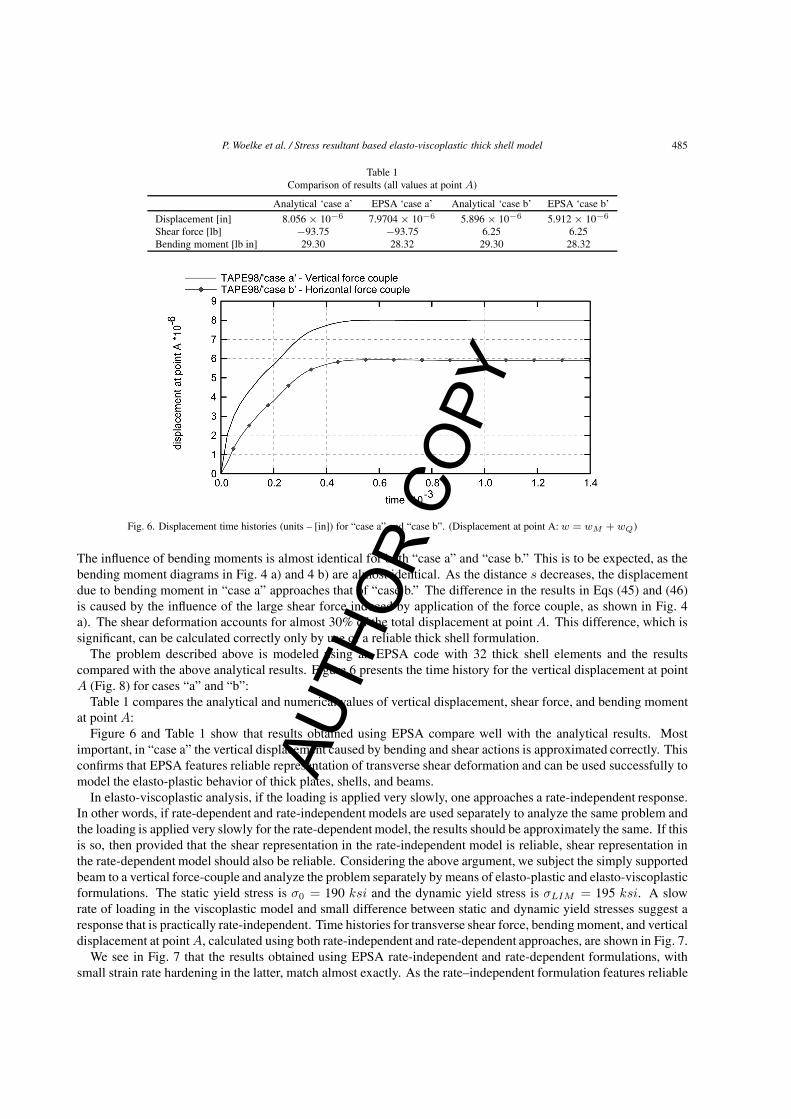
Fig. 6. Displacement time histories (units – [in]) for “case a” and “case b”. (Displacement at point A: w = wM + wQ)

The influence of bending moments is almost identical for both “case a” and “case b.” This is to be expected, as thebending moment diagrams in Fig. 4 a) and 4 b) are almost identical. As the distance s decreases, the displacementdue to bending moment in “case a” approaches that of “case b.” The difference in the results in Eqs (45) and (46)is caused by the influence of the large shear force induced by application of the force couple, as shown in Fig. 4a). The shear deformation accounts for almost 30% of the total displacement at point A. This difference, which issignificant, can be calculated correctly only by use of a reliable thick shell formulation.

The problem described above is modeled using an EPSA code with 32 thick shell elements and the resultscompared with the above analytical results. Figure 6 presents the time history for the vertical displacement at pointA (Fig. 8) for cases “a” and “b”:

Table 1 compares the analytical and numerical values of vertical displacement, shear force, and bending momentat point A:

Figure 6 and Table 1 show that results obtained using EPSA compare well with the analytical results. Mostimportant, in “case a” the vertical displacement caused by bending and shear actions is approximated correctly. Thisconfirms that EPSA features reliable representation of transverse shear deformation and can be used successfully tomodel the elasto-plastic behavior of thick plates, shells, and beams.

In elasto-viscoplastic analysis, if the loading is applied very slowly, one approaches a rate-independent response.In other words, if rate-dependent and rate-independent models are used separately to analyze the same problem andthe loading is applied very slowly for the rate-dependent model, the results should be approximately the same. If thisis so, then provided that the shear representation in the rate-independent model is reliable, shear representation inthe rate-dependent model should also be reliable. Considering the above argument, we subject the simply supportedbeam to a vertical force-couple and analyze the problem separately by means of elasto-plastic and elasto-viscoplasticformulations. The static yield stress is σ0 = 190 ksi and the dynamic yield stress is σLIM = 195 ksi. A slowrate of loading in the viscoplastic model and small difference between static and dynamic yield stresses suggest aresponse that is practically rate-independent. Time histories for transverse shear force, bending moment, and verticaldisplacement at point A, calculated using both rate-independent and rate-dependent approaches, are shown in Fig. 7.

We see in Fig. 7 that the results obtained using EPSA rate-independent and rate-dependent formulations, withsmall strain rate hardening in the latter, match almost exactly. As the rate–independent formulation features reliable

AUTH

OR

COPY


Fig. 7. Time histories of: a) transverse shear force, b) bending moment, and c) vertical displacement at point A, calculated using rate-independentand rate-dependent approaches.

AUTH

OR

COPY


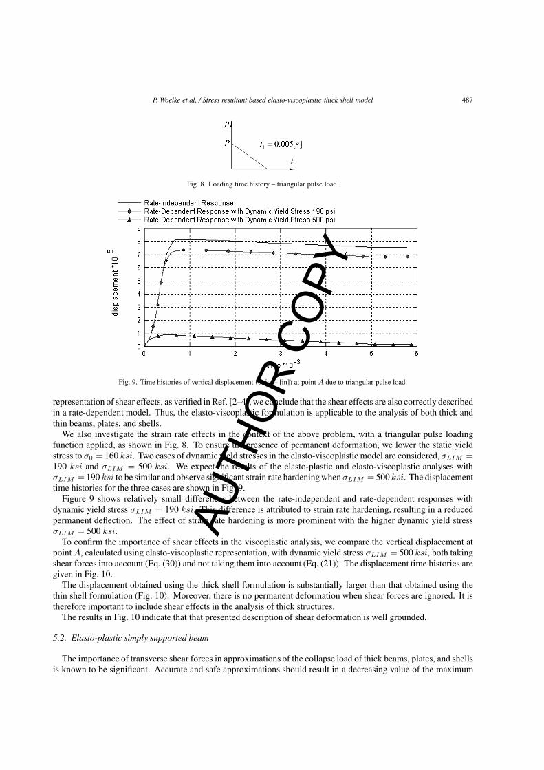
Fig. 8. Loading time history – triangular pulse load.

Fig. 9. Time histories of vertical displacement (units – [in]) at point A due to triangular pulse load.

representation of shear effects, as verified in Ref. [2–4], we conclude that the shear effects are also correctly describedin a rate-dependent model. Thus, the elasto-viscoplastic formulation is applicable to the analysis of both thick andthin beams, plates, and shells.

We also investigate the strain rate effects in the context of the above problem, with a triangular pulse loadingfunction applied, as shown in Fig. 8. To ensure the presence of permanent deformation, we lower the static yieldstress to σ0 = 160 ksi. Two cases of dynamic yield stresses in the elasto-viscoplastic model are considered, σLIM =190 ksi and σLIM = 500 ksi. We expect the results of the elasto-plastic and elasto-viscoplastic analyses withσLIM = 190 ksi to be similar and observe significant strain rate hardeningwhen σLIM = 500 ksi. The displacementtime histories for the three cases are shown in Fig. 9.

Figure 9 shows relatively small differences between the rate-independent and rate-dependent responses withdynamic yield stress σLIM = 190 ksi. This difference is attributed to strain rate hardening, resulting in a reducedpermanent deflection. The effect of strain rate hardening is more prominent with the higher dynamic yield stressσLIM = 500 ksi.

To confirm the importance of shear effects in the viscoplastic analysis, we compare the vertical displacement atpoint A, calculated using elasto-viscoplastic representation, with dynamic yield stress σLIM = 500 ksi, both takingshear forces into account (Eq. (30)) and not taking them into account (Eq. (21)). The displacement time histories aregiven in Fig. 10.

The displacement obtained using the thick shell formulation is substantially larger than that obtained using thethin shell formulation (Fig. 10). Moreover, there is no permanent deformation when shear forces are ignored. It istherefore important to include shear effects in the analysis of thick structures.

The results in Fig. 10 indicate that that presented description of shear deformation is well grounded.

5.2. Elasto-plastic simply supported beam

The importance of transverse shear forces in approximations of the collapse load of thick beams, plates, and shellsis known to be significant. Accurate and safe approximations should result in a decreasing value of the maximum

AUTH

OR

COPY


Fig. 10. Time histories of vertical displacement (units – [in]) at point A due to triangular pulse load – with and without shear effects considered.

Fig. 11. Simply supported beam – geometry, material properties, and results; collapse load as a function of thickness (HOD-Hodge [11]).

load factor with increasing thickness. To test the accuracy of our formulation in accounting for shear deformation,we consider a simply supported beam of length 2L = 10 in, subjected to a concentrated load 2P at its mid-point.Young’s modulus is E = 3.0 x 107 psi, the yield stress is σ0 = 500 psi, and the width of the beam is b = 1 in(Fig. 11). As in the previous example, we model the beam with 32 thick shell elements using EPSA and compute theload factor of the beam as a function of its thickness. The analytical solution of this problem given by Hodge [11]

AUTH

OR

COPY


Fig. 12. Cylindrical shell subjected to a ring of pressure.

Fig. 13. Finite element mesh of an octant of the cylinder.

serves as a reference solution.As seen in Fig. 11, the results obtained with the EPSA thick shell element closely agree with the analytical results

of Hodge [11]. As expected, there is a substantial reduction in the collapse load factor for thick beams. This confirmsthat our representation of shear effects in the elasto-plastic analysis of shells is sound and capable of deliveringaccurate results.

For practical purposes, only a certain range of H is significant. When the thickness of the beam, plate, or shellexceeds 50% of its total length, the problem becomes purely academic, although it is still valuable for illustrativepurposes.

5.3. Cylindrical shell subjected to a ring of pressure

As discussed in the Introduction, the main objective of the current work is to account for the influence of transverseshear strains and stresses on the behavior of shell structures subjected to static and dynamic loads. To further verifythe dependability of the representation of the transverse shear effects, we consider a cylindrical shell under the ringof pressure. The geometry and material parameters are shown in Fig. 12. Due to symmetry, we only consider anoctant of the shell, which is modeled using finite element mesh, as shown in Fig. 13.

We analyze the problem using EPSA shell elements, based on the thin shell formulation, and compare the resultswith those obtained using the same shell elements modified to account for transverse shear deformation. First,we consider a cylinder with thickness t = 0.5 mm. Shells in which the ratio of the radius of the curvature andthickness is higher than 50 usually are considered thin. In this case, the results delivered by EPSA thin-layered shellelement, previously shown to be reliable, will be sufficiently accurate. Solving the problem using the thick layeredshell formulation presented here should therefore produce similar results. We compare the radial displacements atmidspan of the cylinder, determined by thin and thick shell formulations. The time history plots are shown in Fig. 14.

AUTH

OR

COPY


Fig. 14. Radial displacements for a cylinder subjected to a ring of pressure (t = 0.5 mm).

Fig. 15. Radial displacement for a cylinder subjected to a ring of pressure (t = 5 mm).

Figure 14 shows that, as expected, the results produced by the thin and thick shell formulations are practicallyidentical. Shear effects are negligible in this problem, as correctly recognized by the thick shell model.

We increase the thickness of the cylinder to t = 5 mm and the pressure to P = 1.0 kN/mm and again comparethe radial displacements obtained from the two formulations. The displacement time history plots are shown inFig. 15.

Displacement calculated using the current, thick shell formulation is 17% larger than that obtained withoutaccounting for shear stresses. At the same time, the bending moments and axial forces determined by the thick andthin shell formulations are approximately the same (Fig. 16). This significant discrepancy between displacementvalues is attributed to increased influence of the transverse shear effects, which are correctly represented in thecurrent formulation.

6. Conclusion

We introduce transverse shear effects into a viscoplastic model formulated using the finite element code EPSA.Accounting for out-of-plane shear strains and stresses is necessary for accurate modeling of the elastic and plastic,

AUTH

OR

COPY


Fig. 16. Bending moment at midspan of the cylinder subjected to a ring of pressure (t = 5 mm).

rate-dependent behavior of thick plates and shells. A stress-resultant-based, dynamic yield surface is used, withshear forces calculated from transverse shear strains.

EPSA is an explicit code featuring a constant strain shell element. The equation of motion is solved locally,without assembling the stiffness matrix of the structure. Neither shear nor membrane locking is experienced here.The description of the solution procedure of the dynamic equations of motion, as well as the anti-hourglass procedureand other details of he code are discussed in references [1–4,8].

The numerical examples were selected to challenge the most important feature of this work, the representation oftransverse shear effects in elasto-viscoplastic investigations. The beam problems were solved using shell elementswith elasto-plastic and elasto-viscoplastic material representations. The boundary conditions and material propertieswere set such that the problem is a discriminating test of the accuracy of the formulation with respect to descriptionof the shear effects in the viscoplastic shell model.

In all the cases considered, the calculated responses of the structure showed that the formulation is well grounded.The EPSA rate-dependent shell finite element is therefore capable of producing accurate approximations of elasticand elasto-viscoplastic behavior of thin and thick beams, plates, and shells.

References

[1] R.S. Atkatsh, M.L. Baron and M.P. Bieniek, A Finite Difference Variational Method for Bending of Plates, Computers & Structures 11(1980), 573–577.

[2] R.S. Atkatsh, M.P. Bieniek and M.L. Baron, Dynamic Elasto-Plastic Response of Shells in an Acoustic MediumZ – EPSA Code, Int JNum Meth Eng 19(6) (1983), 811–824.

[3] R.S. Atkatsh, M.P. Bieniek and I.S. Sandler, Theory of Viscoplastic Shells for Dynamic Response, J of Applied Mechanics 50 (1983),131–136.

[4] M.P. Bieniek and J.R. Funaro, Elasto-Plastic Behavior of Plates and Shells, Technical report DNA 3584A, Weidlinger Associates, NewYork, 1976.

[5] E.D. Bingham, Fluidity and Plasticity, McGraw-Hill, 1922.[6] S.R. Bodner and Y. Partom, Constitutive Equations for Elastic-Viscoplastic Strain-Herdening Materials, J Appl Mech June (1975), 385–389.[7] D.S. Clark and P.E. Duwez, The influence of Strain Rate on Some Tensile Properties of Steel, Proc Am Soc Testing Materials 50 (1950),

560–575.[8] D.P. Flanagan and T. Belytschko, A uniform strain hexahedron and quadrilateral with orthogonal hourglass control, Int J Num, Meth Eng

17 (1981), 679–706.[9] W. Flugge, Stresses in Shells, Springer, New York, 1960.

[10] H.-C. Hu, Variational Principles of Theory of Elasticity with Applications, Scientific Publisher, Beijing, China, 1984.[11] P.G. Hodge, Plastic Analysis of Structures, McGraw-Hill, 1959.[12] A.A. Iliushin, Plastichnost’, Gostekhizdat, Moscow, 1956.

AUTH

OR

COPY


[13] W.B. Kratzig, ‘Best’ transverse shearing and stretching shelll theory for nonlinear finite element simulations, Comp Meth Appl Mech Eng103 (1992), 135–160.

[14] U.S. Lindholm, Review of Dynamic Testing Techniques and Material Behavior, Conference on Mechanical Properties of Materials at HighRates of Strain, Institute of Physics, London, 1974.

[15] E. Onate, A review of some finite element families for thick and thin plate and shell analysis, in: Recent Developments in FE Analysis,T.J.R. Hughes, E. Onate, and O.C. Zienkiewicz, eds, CIMNE: Barcelona, 1999.

[16] P. Perzyna, Fundamental Problems in Viscoplasticity, Advances in Applied Mechanics 9 (1966), 243–377.[17] E. Reissner, The effects of transverse shear deformation on the bending of elastic plates, J Appl Mech ASME 12 (1945), 66–77.[18] E. Reissner, On transverse bending of plates, including the effects of transverse shear deformation, Int J Solids Structures 11 (1975),

569–576.[19] M. Robinson, A comparison of yield surfaces for thin shells, Int J Mech Sci 13 (1971), 345–354.[20] G.S. Shapiro, On yield surface for ideally plastic shells. In Problems of Continuous Mechanics, SIAM, Philadelphia, 1961, 414–418.[21] G. Shi and G.Z. Voyiadjis, A simple non-layered finite element for the elasto-plastic analysis of shear flexible plates, Int J Num Meth

Engng 33 (1992), 85–99.[22] J.C. Simo, D.D. Fox and M.S. Rifai, On a stress resultant geometrically exact shell model, Part II: The linear Theory 73 (1989), 53–92; Part

III: Computational Aspects of the Nonlinear Theory 79, 21–70. Computer Methods in Applied Mechanics and Engineering. North-Holland.[23] P. Woelke, G.Z. Voyiadjis and P. Perzyna, Elasto-plastic finite element analysis of shells with damage due to microvoids, Int J Num Meth

Eng 68(3) (2006), 338–380.[24] G.Z. Voyiadjis and P. Woelke, General non-linear finite element analysis of thick plates and shells, Int J Solids Structures 43(Issue 7–8, 1)

(2005), 2209–2242.[25] G.Z. Voyiadjis and P. Woelke, (2009), Elasto-Plastic and Damage Analysis of Plates and Shells, Springer 2008.[26] G.A. Wempner, Nonlinear Theory of Shells, ASCE National Environmental Engineering Meeting, New York, 1973.

AUTH

OR

COPY

Documents

Stress Resultant Based Elasto-Viscoplastic Thick Shell Model