arX

iv:1

401.

2247

v1 [

mat

h.PR

] 1

0 Ja

n 20

14

Strong asymptotic independence

on Wiener chaos

Ivan Nourdin∗, David Nualart† and Giovanni Peccati‡

January 13, 2014

Abstract

Let Fn = (F1,n, ...., Fd,n), n > 1, be a sequence of random vectors such that, forevery j = 1, ..., d, the random variable Fj,n belongs to a fixed Wiener chaos of aGaussian field. We show that, as n → ∞, the components of Fn are asymptoticallyindependent if and only if Cov(F 2

i,n, F2j,n) → 0 for every i 6= j. Our findings are based

on a novel inequality for vectors of multiple Wiener-Itô integrals, and represent asubstantial refining of criteria for asymptotic independence in the sense of momentsrecently established by Nourdin and Rosiński [9].Keywords: Gaussian Fields; Independence; Limit Theorems; Malliavin calculus;Wiener Chaos.2000 Mathematics Subject Classification: 60F05, 60H07, 60G15.

1 Introduction

1.1 Overview

Let X = X(h) : h ∈ H be an isonormal Gaussian process over some real separable Hilbertspace H (see Section 1.2 and Section 2 for relevant definitions), and let Fn = (F1,n, ...., Fd,n),n > 1, be a sequence of random vectors such that, for every j = 1, ..., d, the random variableFj,n belongs the qjth Wiener chaos of X (the order qj > 1 of the chaos being independentof n). The following result, proved by Nourdin and Rosiński in [9, Corollary 3.6], providesa useful criterion for the asymptotic independence of the components of Fn.

Theorem 1.1 (See [9]) Assume that, as n→ ∞ and for every i 6= j,

Cov(F 2i,n, F

2j,n) → 0 and Fj,n

law→ Uj , (1.1)

∗Email: inourdin@gmail.com; IN was partially supported by the ANR Grant ANR-10-BLAN-0121.†Email: nualart@math.ku.edu; DN was partially supported by the NSF grant DMS1208625.‡Email: giovanni.peccati@gmail.com; GP was partially supported by the grant F1R-MTH-PUL-

12PAMP (PAMPAS), from Luxembourg University.

1

where each Uj is a moment-determinate∗ random variable. Then,

Fnlaw−→ (U1, . . . , Ud),

where the Uj’s are assumed to be mutually stochastically independent.

In words, Theorem 1.1 allows one to deduce joint convergence from the component-wise convergence of the elements of Fn, provided the limit law of each sequence Fj,nis moment-determinate and the covariances between the squares of the distinct compo-nents of Fn vanish asymptotically. This result and its generalisations have already led tosome important applications, notably in connection with time-series analysis and with theasymptotic theory of homogeneous sums — see [1, 2, 9]. The aim of this paper is to studythe following important question, which was left open in the reference [9]:

Question A. In the statement of Theorem 1.1, is it possible to remove the moment-determinacy assumption for the random variables U1, ..., Ud?

Question A is indeed very natural. For instance, it is a well-known fact (see [14, Section3]) that non-zero random variables living inside a fixed Wiener chaos of order q > 3 arenot necessarily moment-determinate, so that Theorem 1.1 cannot be applied in severalcontexts where the limit random variables Uj have a chaotic nature. Until now, such ashortcoming has remarkably restricted the applicability of Theorem 1.1 — see for instancethe discussion contained in [1, Section 3].

In what follows, we shall derive several new probabilistic estimates (stated in Section1.3 below) for chaotic random variables, leading to a general positive answer to QuestionA. As opposed to the techniques applied in [9], our proof does not make use of combi-natorial arguments. Instead, we shall heavily rely on the use of Malliavin calculus andMeyer inequalities (see the forthcoming formula (2.11)). This new approach will yield sev-eral quantitative extensions of Theorem 1.1, each having its own interest. Note that, inparticular, our main results immediately confirm Conjecture 3.7 in [1].

The content of the present paper represents a further contribution to a recent and veryactive direction of research, revolving around the application of Malliavin-type techniquesfor deriving probabilistic approximations and limit theorems, with special emphasis onnormal approximation results (see [11, 13] for two seminal contributions to the field, aswell as [8] for recent developments).The reader is referred to the book [7] and the survey[4] for an overview of this area of research. One can also consult the constantly updatedwebpage [5] for literally hundreds of results related to the findings contained in [11, 13]and their many ramifications.

1.2 Some basic definitions and notation

We refer the reader to [7, 10] for any unexplained definition or result.

∗Recall that a random variable U with moments of all orders is said to be moment-determinate ifE[Xn] = E[Un] for every n = 1, 2, ... implies that X and U have the same distribution.

2

Let H be a real separable infinite-dimensional Hilbert space. For any integer q > 1, letH⊗q be the qth tensor product of H. Also, we denote by H⊙q the qth symmetric tensorproduct. From now on, the symbol X = X(h) : h ∈ H will indicate an isonormalGaussian process on H, defined on some probability space (Ω,F , P ). In particular, X is acentered Gaussian family with covariance given by E[X(h)X(g)] = 〈h, g〉H. We will alsoassume that F is generated by X.

For every integer q > 1, we let Hq be the qth Wiener chaos of X, that is, Hq is theclosed linear subspace of L2(Ω) generated by the class Hq(X(h)) : h ∈ H, ‖h‖

H= 1,

where Hq is the qth Hermite polynomial defined by

Hq(x) =(−1)q

q!ex

2/2 dq

dxq

(e−x2/2

).

We denote by H0 the space of constant random variables. For any q > 1, the mappingIq(h

⊗q) = q!Hq(X(h)) can be extended a linear isometry between H⊙q (equipped withthe modified norm

√q! ‖·‖

H⊗q) and Hq (equipped with the L2(Ω) norm). For q = 0, byconvention H0 = R, and I0 is the identity map.

It is well-known (Wiener chaos expansion) that L2(Ω) can be decomposed into theinfinite orthogonal sum of the spaces Hq, that is: any square-integrable random variableF ∈ L2(Ω) admits the following chaotic expansion:

F =

∞∑

q=0

Iq(fq), (1.2)

where f0 = E[F ], and the fq ∈ H⊙q, q > 1, are uniquely determined by F . For everyq > 0, we denote by Jq the orthogonal projection operator on the qth Wiener chaos. Inparticular, if F ∈ L2(Ω) is as in (1.2), then JqF = Iq(fq) for every q > 0.

1.3 Main results

The main achievement of the present paper is the explicit estimate (1.3), appearing in theforthcoming Theorem 1.2. Note that, in order to obtain more readable formulae, we onlyconsider multiple integrals with unit variance: one can deduce bounds in the general caseby a standard rescaling procedure.

Remark on notation. Fix integers m, q > 1. Given a smooth function ϕ : Rm → R, weshall use the notation

‖ϕ‖q := ‖ϕ‖∞ +∑

∥∥∥∥∥∂kϕ

∂xk1i1 · · ·∂xkpip

∥∥∥∥∥∞

,

where the sum runs over all p = 1, ..., m, all i1, ..., ip ⊂ 1, ..., m, and all multi indices(k1, ..., kp) ∈ 1, 2, ...p verifying k1 + · · ·+ kp := k 6 q.

3

Theorem 1.2 Let d > 2 and let q1 > q2 > · · · > qd > 1 be fixed integers. There exists aconstant c, uniquely depending on d and (q1, ..., qd), verifying the following bound for anyd-dimensional vector

F = (F1, ..., Fd),

such that Fj = Iqj(fj), fj ∈ H⊙qj (j = 1, ..., d) and E[F 2j ] = 1 for j = 1, ..., d − 1, and for

any collection of smooth test functions ψ1, ..., ψd : R → R,∣∣∣∣∣E[

d∏

j=1

ψj(Fj)

]−

d∏

j=1

E[ψj(Fj)]

∣∣∣∣∣ 6 c ‖ψ′d‖∞

d−1∏

j=1

‖ψj‖q1∑

16j<ℓ6d

Cov(F 2j , F

2ℓ ). (1.3)

When applied to sequences of multiple stochastic integrals, Theorem 1.2 allows one todeduce the following strong generalization of [9, Theorem 3.4].

Theorem 1.3 Let d > 2 and let q1 > q2 > · · · > qd > 1 be fixed integers. For everyn > 1, let Fn = (F1,n, ..., Fd,n) be a d-dimensional random vector such that Fj,n = Iqj(fj,n),with fj,n ∈ H⊙qj and E[F 2

j,n] = 1 for all 1 6 j 6 d and n > 1. Then, the following threeconditions are equivalent, as n→ ∞:

(1) Cov(F 2i,n, F

2j,n) → 0 for every 1 6 i 6= j 6 d;

(2) ‖fi,n ⊗r fj,n‖ → 0 for every 1 6 i 6= j 6 d and 1 6 r 6 qi ∧ qj;

(3) The random variables F1,n, ..., Fd,n are asymptotically independent, that is, for everycollection of smooth bounded test functions ψ1, ..., ψd : R → R,

E

[d∏

j=1

ψj(Fj,n)

]−

d∏

j=1

E[ψj(Fj,n)] −→ 0.

We can now state the announced extension of Theorem 1.1 (see Section 1), in whichthe determinacy condition for the limit random variables Uj has been eventually removed.

Theorem 1.4 Let d > 2 and let q1 > q2 > · · · > qd > 1 be fixed integers. For every n > 1,let Fn = (F1,n, ..., Fd,n) be a d-dimensional random vector such that Fj,n = Iqj(fj,n), withfj,n ∈ H⊙qj and E[F 2

j,n] = 1 for all 1 6 j 6 d and n > 1. Let U1, . . . , Ud be independent

random variables such that Fj,nlaw→ Uj as n→ ∞ for every 1 6 j 6 d. Assume that either

Condition (1) or Condition (2) of Theorem 1.3 holds. Then, as n→ ∞,

Fnlaw→ (U1, . . . , Ud).

By considering linear combinations, one can also prove the following straightforwardgeneralisations of Theorem 1.3 and Theorem 1.4 (which are potentially useful for applica-tions), where each component of the vector Fn is replaced by a multidimensional object.The simple proofs are left to the reader.

4

Proposition 1.5 Let d > 2, let q1 > q2 > · · · > qd > 1 and m1, ..., md > 1 be fixedintegers, and set M :=

∑dj=1mj. For every j = 1, ..., d, let

Fj,n = (F(1)j,n , ..., F

(mj)j,n ) :=

(Iqj(f

(1)j,n ), ..., Iqj(f

(mj)j,n )

),

where, for ℓ = 1, ..., mj, f(ℓ)j,n ∈ H⊙qj and E[(F

(ℓ)j,n)

2] = qj !‖f (ℓ)j,n‖2H⊗qj

= 1. Finally, for every

n > 1, write Fn to indicate the M-dimensional vector (F1,n, ...,Fd,n). Then, the followingthree conditions are equivalent, as n→ ∞:

(1) Cov((F

(ℓ)i,n )

2, (F(ℓ′)j,n )2

)→ 0 for every 1 6 i 6= j 6 d, every ℓ = 1, ..., mi and every

ℓ′ = 1, ..., mj;

(2) ‖f (ℓ)i,n ⊗r f

(ℓ′)j,n ‖ → 0 for every 1 6 i 6= j 6 d, for every 1 6 r 6 qi ∧ qj, every

ℓ = 1, ..., mi and every ℓ′ = 1, ..., mj;

(3) The random vectors F1,n, ...,Fd,n are asymptotically independent, that is: for everycollection of smooth bounded test functions ψj : R

mj → R, j = 1, ..., d,

E

[d∏

j=1

ψj(Fj,n)

]−

d∏

j=1

E[ψj(Fj,n)] −→ 0.

Proposition 1.6 Let the notation and assumptions of Proposition 1.5 prevail, and as-sume that either Condition (1) or Condition (2) therein is satisfied. Consider a collection(U1, ...,Ud) of independent random vectors such that, for j = 1, ..., d, Uj has dimensionmj. Then, if Fj,n converges in distribution to Uj, as n→ ∞, one has also that

Fnlaw→ (U1, . . . ,Ud).

The plan of the paper is as follows. Section 2 contains some further preliminaries relatedto Gaussian analysis and Malliavin calculus. The proofs of our main results are gatheredin Section 3.

2 Further notation and results from Malliavin calculus

Let ek, k > 1 be a complete orthonormal system in H. Given f ∈ H⊙p, g ∈ H⊙q andr ∈ 0, . . . , p ∧ q, the rth contraction of f and g is the element of H⊗(p+q−2r) defined by

f ⊗r g =

∞∑

i1,...,ir=1

〈f, ei1 ⊗ . . .⊗ eir〉H⊗r ⊗ 〈g, ei1 ⊗ . . .⊗ eir〉H⊗r . (2.4)

Notice that f ⊗r g is not necessarily symmetric. We denote its symmetrization by f⊗rg ∈H⊙(p+q−2r). Moreover, f ⊗0 g = f ⊗g equals the tensor product of f and g while, for p = q,

5

f ⊗q g = 〈f, g〉H⊗q . In the particular case H = L2(A,A, µ), where (A,A) is a measurablespace and µ is a σ-finite and non-atomic measure, one has that H⊙q can be identifiedwith the space L2

s(Aq,A⊗q, µ⊗q) of µq-almost everywhere symmetric and square-integrable

functions on Aq. Moreover, for every f ∈ H⊙q, Iq(f) coincides with the multiple Wiener-Itôintegral of order q of f with respect to X and (2.4) can be written as

(f ⊗r g)(t1, . . . , tp+q−2r) =

∫

Ar

f(t1, . . . , tp−r, s1, . . . , sr)

× g(tp−r+1, . . . , tp+q−2r, s1, . . . , sr)dµ(s1) . . . dµ(sr).

We will now introduce some basic elements of the Malliavin calculus with respect tothe isonormal Gaussian process X (see again [7, 10] for any unexplained notion or result).Let S be the set of all smooth and cylindrical random variables of the form

F = g (X(φ1), . . . , X(φn)) , (2.5)

where n > 1, g : Rn → R is a infinitely differentiable function with compact support, andφi ∈ H. The Malliavin derivative of F with respect to X is the element of L2(Ω,H) definedas

DF =

n∑

i=1

∂g

∂xi(X(φ1), . . . , X(φn))φi.

By iteration, one can define the qth derivative DqF for every q > 2, which is an elementof L2(Ω,H⊙q).

For q > 1 and p > 1, Dq,p denotes the closure of S with respect to the norm ‖ · ‖Dq,p,defined by the relation

‖F‖pDq,p = E [|F |p] +

q∑

i=1

E[‖DiF‖p

H⊗i

].

The Malliavin derivative D verifies the following chain rule. If ϕ : Rn → R is continu-ously differentiable with bounded partial derivatives and if F = (F1, . . . , Fn) is a vector ofelements of D1,2, then ϕ(F ) ∈ D

1,2 and

Dϕ(F ) =

n∑

i=1

∂ϕ

∂xi(F )DFi. (2.6)

Note also that a random variable F as in (1.2) is in D1,2 if and only if

∞∑

q=1

qq!‖fq‖2H⊗q <∞,

6

and, in this case, E [‖DF‖2H] =∑

q>1 qq!‖fq‖2H⊗q . If H = L2(A,A, µ) (with µ non-atomic),then the derivative of a random variable F as in (1.2) can be identified with the elementof L2(A× Ω) given by

DaF =∞∑

q=1

qIq−1 (fq(·, a)) , a ∈ A. (2.7)

We denote by δ the adjoint of the operator D, also called the divergence operator. Arandom element u ∈ L2(Ω,H) belongs to the domain of δ, noted Dom δ, if and only if itverifies

∣∣E[〈DF, u〉H

]∣∣ 6 cu√E[F 2]

for any F ∈ D1,2, where cu is a constant depending only on u. If u ∈ Dom δ, then the

random variable δ(u) is defined by the duality relationship (customarily called ‘integrationby parts formula’):

E[Fδ(u)] = E[〈DF, u〉H

], (2.8)

which holds for every F ∈ D1,2. The formula (2.8) extends to the multiple Skorohod

integral δq, and we have

E [Fδq(u)] = E[〈DqF, u〉

H⊗q

](2.9)

for any element u in the domain of δq and any random variable F ∈ Dq,2. Moreover,

δq(h) = Iq(h) for any h ∈ H⊙q.

The following property, corresponding to [6, Lemma 2.1], will be used in the paper. Letq > 1 be an integer, suppose that F ∈ D

q,2, and let u be a symmetric element in Dom δq.Assume that 〈DrF, δj(u)〉

H⊗r ∈ L2(Ω,H⊗q−r−j) for any 0 6 r + j 6 q. Then 〈DrF, u〉H⊗r

belongs to the domain of δq−r for any r = 0, . . . , q − 1, and we have

Fδq(u) =

q∑

r=0

(q

r

)δq−r

(〈DrF, u〉

H⊗r

). (2.10)

(We use the convention that δ0(v) = v, v ∈ R, and D0F = F , F ∈ L2(Ω).)

For any Hilbert space V , we denote by Dk,p(V ) the corresponding Sobolev space of V -

valued random variables (see [10, page 31]). The operator δq is continuous from Dk,p(H⊗q)

to Dk−q,p, for any p > 1 and any integers k ≥ q ≥ 1, and one has the estimate

‖δq(u)‖Dk−q,p 6 ck,p ‖u‖Dk,p(H⊗q) (2.11)

for all u ∈ Dk,p(H⊗q), and some constant ck,p > 0. These inequalities are direct con-

sequences of the so-called Meyer inequalities (see [10, Proposition 1.5.7]). In particular,these estimates imply that Dq,2(H⊗q) ⊂ Dom δq for any integer q ≥ 1.

7

The operator L is defined on the Wiener chaos expansion as

L =∞∑

q=0

−qJq,

and is called the infinitesimal generator of the Ornstein-Uhlenbeck semigroup. The domainof this operator in L2(Ω) is the set

DomL = F ∈ L2(Ω) :∞∑

q=1

q2 ‖JqF‖2L2(Ω) <∞ = D2,2.

There is an important relationship between the operatorsD, δ and L. A random variable Fbelongs to the domain of L if and only if F ∈ Dom(δD) (i.e. F ∈ D

1,2 and DF ∈ Dom δ),and in this case

δDF = −LF. (2.12)

We also define the operator L−1, which is the pseudo-inverse of L, as follows: for everyF ∈ L2(Ω) with zero mean, we set L−1F =

∑q>1−1

qJq(F ). We note that L−1 is an operator

with values in D2,2 and that LL−1F = E − E[F ] for any F ∈ L2(Ω).

3 Proofs of the results stated in Section 1.3

3.1 Proof of Theorem 1.2

The proof of Theorem 1.2 is based on a recursive application of the following quantitativeresult, whose proof has been inspired by the pioneering work of Üstünel and Zakai on thecharacterization of the independence on Wiener chaos (see [15]).

Proposition 3.1 Let m > 1 and p1, ..., pm, q be integers such that pj > q for every j =1, ..., m. There exists a constant c, uniquely depending on m and p1, ..., pm, q, such that onehas the bound

|E[ϕ(F )ψ(G)]− E[ϕ(F )]E[ψ(G)]| ≤ c‖ψ′‖∞‖ϕ‖qm∑

j=1

Cov(F 2j , G

2),

for every vector F = (F1, ..., Fm) such that Fj = Ipj(fj), fj ∈ H⊙pj and E[F 2j ] = 1

(j = 1, ..., m), for every random variable G = Iq(g), g ∈ H⊙q, and for every pair of smoothtest functions ϕ : Rm → R and ψ : R → R.

Proof. Throughout the proof, the symbol c will denote a positive finite constant uniquelydepending on m and p1, ..., pm, q, whose value may change from line to line. Using the chainrule (2.6) together with the relation −DL−1 = (I − L)−1D (see, e.g., [12]), one has

ϕ(F )− E[ϕ(F )] = LL−1ϕ(F ) = −δ(DL−1ϕ(F )) =m∑

j=1

δ((I − L)−1∂jϕ(F )DFj),

8

from which one deduces that

E[ϕ(F )ψ(G)]− E[ϕ(F )]E[ψ(G)] =m∑

j=1

E[〈(I − L)−1∂jϕ(F )DFj, DG〉Hψ′(G)]

≤ ‖ψ′‖∞m∑

j=1

E[|〈(I − L)−1∂jϕ(F )DFj, DG〉H|

].

We shall now fix j = 1, ..., m, and consider separately every addend appearing in the pre-vious sum. As it is standard, without loss of generality, we can assume that the underlyingHilbert space H is of the form L2(A,A, µ), where µ is a σ-finite measure without atoms.It follows that

〈(I−L)−1∂jϕ(F )DFj, DG〉H = pjq

∫

A

[(I−L)−1∂jϕ(F )Ipj−1(fj(·, θ))]Iq−1(g(·, θ))µ(dθ).

(3.13)

Now we apply the formula (2.10) to u = g(·, θ) and F = (I−L)−1∂jϕ(F )Ipj−1(fj(·, θ)) andwe obtain, using Dr(I − L)−1 = ((r + 1)I − L)−1Dr as well (see, e.g., [12]),

[(I − L)−1∂jϕ(F )Ipj−1(fj(·, θ))]Iq−1(g(·, θ)) (3.14)

=

q−1∑

r=0

(q − 1

r

)δq−1−r

(⟨g(·, θ), Dr[(I − L)−1∂jϕ(F )Ipj−1(fj(·, θ))]

⟩H⊗r

)

=

q−1∑

r=0

(q − 1

r

)δq−1−r

(⟨g(·, θ), ((r + 1)I − L)−1Dr[∂jϕ(F )Ipj−1(fj(·, θ))]

⟩H⊗r

).

Now, substituting (3.14) into (3.13) yields

〈(I − L)−1∂jϕ(F )DFj, DG〉H = pjq

q−1∑

r=0

(q − 1

r

)

×δq−1−r

(∫

Ar+1

g(·, sr+1)((r + 1)I − L)−1Drs1,...,sr [∂jϕ(F )Ipj−1(fj(·, sr+1))]µ(ds

r+1)

),

where sr+1 = (s1, . . . , sr+1). We have, by the Leibniz rule,

Drs1,...,sr

[∂jϕ(F )Ipj−1(fj(·, sr+1))] =

r∑

α=0

(r

α

)Dα

s1,...,sα[∂jϕ(F )]D

r−αsα+1,...,sr

[Ipj−1(fj(·, sr+1))]

=

r∑

α=0

(r

α

)(pj − 1)!

(pj − r + α− 1)!Dα

s1,...,sα[∂jϕ(F )]Ipj−r+α−1(fj(·, sα+1, . . . , sr+1)).

Fix 0 ≤ r ≤ q − 1 and 0 ≤ α ≤ r. It suffices to estimate the following expectation

E

∣∣∣∣∣δq−1−r

(∫

Ar+1

g(·, sα, tr−α+1) (3.15)

×((r + 1)I − L)−1Dαsα [∂jϕ(F )]Ipj−r+α−1(fj(·, tr−α+1))µ(dsα)µ(dtr−α+1)

)∣∣∣∣∣.

9

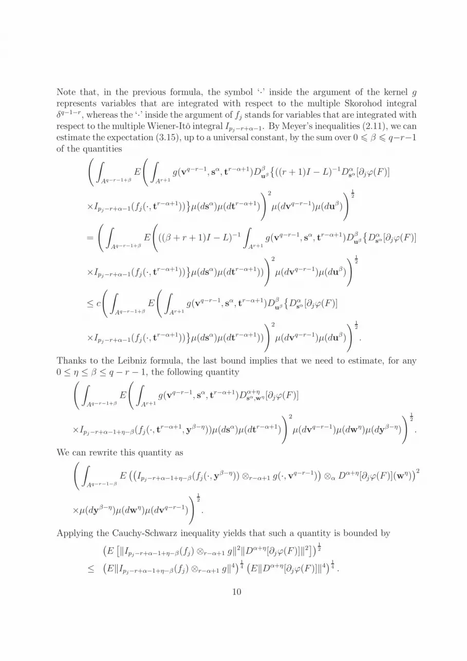
Note that, in the previous formula, the symbol ‘·’ inside the argument of the kernel grepresents variables that are integrated with respect to the multiple Skorohod integralδq−1−r, whereas the ‘·’ inside the argument of fj stands for variables that are integrated withrespect to the multiple Wiener-Itô integral Ipj−r+α−1. By Meyer’s inequalities (2.11), we canestimate the expectation (3.15), up to a universal constant, by the sum over 0 6 β 6 q−r−1of the quantities

(∫

Aq−r−1+β

E

(∫

Ar+1

g(vq−r−1, sα, tr−α+1)Dβuβ

((r + 1)I − L)−1Dα

sα[∂jϕ(F )]

×Ipj−r+α−1(fj(·, tr−α+1))µ(dsα)µ(dtr−α+1)

)2

µ(dvq−r−1)µ(duβ)

) 1

2

=

(∫

Aq−r−1+β

E

(((β + r + 1)I − L)−1

∫

Ar+1

g(vq−r−1, sα, tr−α+1)Dβuβ

Dα

sα[∂jϕ(F )]

×Ipj−r+α−1(fj(·, tr−α+1))µ(dsα)µ(dtr−α+1))

)2

µ(dvq−r−1)µ(duβ)

) 1

2

≤ c

(∫

Aq−r−1+β

E

(∫

Ar+1

g(vq−r−1, sα, tr−α+1)Dβuβ

Dα

sα [∂jϕ(F )]

×Ipj−r+α−1(fj(·, tr−α+1))µ(dsα)µ(dtr−α+1))

)2

µ(dvq−r−1)µ(duβ)

) 1

2

.

Thanks to the Leibniz formula, the last bound implies that we need to estimate, for any0 ≤ η ≤ β ≤ q − r − 1, the following quantity

(∫

Aq−r−1+β

E

(∫

Ar+1

g(vq−r−1, sα, tr−α+1)Dα+ηsα,wη [∂jϕ(F )]

×Ipj−r+α−1+η−β(fj(·, tr−α+1,yβ−η))µ(dsα)µ(dtr−α+1)

)2

µ(dvq−r−1)µ(dwη)µ(dyβ−η)

) 1

2

.

We can rewrite this quantity as(∫

Aq−r−1−β

E((Ipj−r+α−1+η−β(fj(·,yβ−η))⊗r−α+1 g(·,vq−r−1)

)⊗α D

α+η[∂jϕ(F )](wη))2

×µ(dyβ−η)µ(dwη)µ(dvq−r−1)

) 1

2

.

Applying the Cauchy-Schwarz inequality yields that such a quantity is bounded by(E[‖Ipj−r+α−1+η−β(fj)⊗r−α+1 g‖2‖Dα+η[∂jϕ(F )]‖2

]) 1

2

≤(E‖Ipj−r+α−1+η−β(fj)⊗r−α+1 g‖4

) 1

4(E‖Dα+η[∂jϕ(F )]‖4

) 1

4 .

10

Set γ = α + η. Applying the generalized Faá di Bruno’s formula (see, e.g., [3]) we deducethat

Dγ[∂jϕ(F )] =∑ γ!∏γ

i=1 i!ki∏γ

i=1

∏mj=1 qij!

∂k∂jϕ(F )

∂xp11 · · ·∂xpmm

γ∧p∗∏

i=1

(DiF1)⊗qi1⊗· · ·⊗(DiFm)

⊗qim,

where p∗ = minp1, ..., pm, and the sum runs over all nonnegative integer solutions of thesystem of γ + 1 equations

k1 + 2k2 + · · ·+ γkγ = γ,

q11 + q12 + · · ·+ q1m = k1,

q21 + q22 + · · ·+ q2m = k2,

· · · · · ·qγ1 + qγ2 + · · ·+ qγm = kγ,

and we have moreover set pj = q1j+· · ·+qγj , j = 1, ..., r, and k = p1+· · ·+pm = k1+· · ·+kγ .This expression yields immediately that

‖Dγ[∂jϕ(F )]‖ ≤ c‖ϕ‖q∑ γ∧p∗∏

i=1

‖DiF1‖qi1 · · · ‖DiFm‖qim

and using the facts that all Dk,p norms (k, p > 1) are equivalent on a fixed Wiener chaosand that the elements of the vector F have unit variance by assumption, we infer that

(E‖Dγ[∂jϕ(F )]‖4

) 1

4 ≤ c‖ϕ‖q.

On the other hand, using hypercontractivity one has that

(E‖Ipj−r+α−1+η−β(fj)⊗r−α+1 g‖4

) 1

4 ≤ c(E‖Ipj−r+α−1+η−β(fj)⊗r−α+1 g‖2

) 1

2 .

Since

E‖Ipj−r+α−1+η−β(fj)⊗r−α+1 g‖2 = (pj − r + α− 1 + η − β)!‖fj ⊗r−α+1 g‖2,

and

max1≤r≤q

‖fj ⊗r g‖ 6 Cov(F 2j , G

2) (see, e.g., [9, inequality (3.26)]),

we finally obtain

E|〈(I − L)−1∂jϕ(F )DFj, DG〉H| ≤ c‖ϕ‖qCov(F 2j , G

2),

thus concluding the proof.

11

Proof of Theorem 1.2. Just observe that

∣∣∣∣∣E[

d∏

j=1

ψj(Fj)

]−

d∏

j=1

E[ψj(Fj)]

∣∣∣∣∣

6

d∑

j=2

∣∣∣E[ψ1(F1) · · ·ψj−1(Fj−1)]E[ψj(Fj)] · · · E[ψd(Fd)]

−E[ψ1(F1) · · ·ψj(Fj)]E[ψj+1(Fj+1)] · · · E[ψd(Fd)]∣∣∣,

so that the conclusion is achieved (after some routine computations) by applying Proposi-tion 3.1 (in the case m = j − 1, pi = qi, i = 1, ..., j − 1, and q = qj) to each summand onthe right-hand side of the previous estimate.

3.2 Proof of Theorem 1.3

The equivalence between (1) and (2) follows from [9, Theorem 3.4]. That (3) implies (1)would have been immediate if the square function x 7→ x2 were bounded. To overcome thisslight difficulty, it suffices to combine the hypercontractivity property of chaotic randomvariables (from which it follows that our sequence (Fn) is bounded in Lp(Ω) for any p > 1)with a standard approximation argument. Finally, the implication (1) ⇒ (3) is a directconsequence of (1.3).

3.3 Proof of Theorem 1.4

Assume that there exists a subsequence of Fn converging in distribution to some limit(V1, . . . , Vd). For any collection of smooth test functions ψ1, ..., ψd : R → R, one can thenwrite

E

[d∏

j=1

ψj(Vj)

]=

d∏

j=1

E [ψj(Vj)] =

d∏

j=1

E [ψj(Uj)] = E

[d∏

j=1

ψj(Uj)

]. (3.16)

Indeed, the first equality in (3.16) is a direct consequence of Theorem 1.3, the second one

follows from the fact that Vjlaw= Uj for any j by assumption, and the last one follows

from the independence of the Uj . Thus, we deduce from (3.16) that (U1, . . . , Ud) is theonly possible limit in law for any converging subsequence extracted from Fn. Since

the sequence Fn is tight (indeed, it is bounded in L2(Ω)), one deduces that Fnlaw→

(U1, . . . , Ud), which completes the proof of Theorem 1.4.

12

References

[1] S. Bai and M.S. Taqqu (2013): Multivariate limit theorems in the context of long-rangedependence. J. Time Series Anal. 34, no. 6, 717-743.

[2] S. Bourguin and J.-C. Breton (2013): Asymptotic Cramér type decomposition forWiener and Wigner integrals. Infinite Dimensional Analysis, Quantum Probabilityand Related Topics 16, no. 1.

[3] R.L. Mishkov (2000): Generalization of the formula of Faa di Bruno for a compositefunction with a vector argument. Internat. J. Math. & Math. Sci. 24, no. 7, 481-491.

[4] I. Nourdin (2012): Lectures on Gaussian approximations with Malliavin calculus. Sém.Probab. XLV, 3-89.

[5] I. Nourdin: A webpage on Stein’s method and Malliavin calculus.https://sites.google.com/site/malliavinstein

[6] I. Nourdin and D. Nualart (2010): Central limit theorems for multiple Skorohodintegrals. J. Theoret. Probab. 23, no 1, 39-64.

[7] I. Nourdin and G. Peccati (2012): Normal Approximations using Malliavin Calculus:from Stein’s Method to the Universality. Cambridge University Press.

[8] I. Nourdin and G. Peccati (2013): The optimal fourth moment theorem. To appearin: Proceedings of the American Mathematical Society.

[9] I. Nourdin and J. Rosiński (2013): Asymptotic independence of multiple Wiener-Itôintegrals and the resulting limit laws. To appear in: Ann. Probab.

[10] D. Nualart (2006): The Malliavin calculus and related topics. Springer-Verlag, Berlin,2nd edition.

[11] D. Nualart and G. Peccati (2005): Central limit theorems for sequences of multiplestochastic integrals. Ann. Probab., 33, no 1, 177-193.

[12] D. Nualart and M. Zakai (1989): A summary of some identities of the Malliavincalculus. Stochastic Partial Differential Equations and Applications II, Lecture Notesin Mathematics 1390, 192-196.

[13] G. Peccati and C.A. Tudor (2004): Gaussian limits for vector-valued multiple stochas-tic integrals. Séminaire de Probabilités XXXVIII, 247-262.

[14] E.V. Slud (1993): The moment problem for polynomial forms in normal randomvariables. Ann. Probab. 21, no 4, 2200-2214.

[15] A. S. Üstünel and M. Zakai (1989): On independence and conditioning on Wienerspace. Ann. Probab., 17, no 4. 1441-1453.

13