arX

iv:h

ep-t

h/96

0506

6v1

10

May

199

6

UB-ECM-PF 96/9 La Plata-Th 96/07

Supersymmetric Electroweak Cosmic Strings

Jose D. Edelsteina ∗ and Carlos Nunezb †

a Departament d’Estructura i Consituents de la Materia

Facultat de Fısica, Universitat de Barcelona

Diagonal 647, 08028 Barcelona, Spain

and

b Departamento de Fısica, Universidad Nacional de La Plata

C.C. 67, (1900) La Plata, Argentina

Abstract

We study the connection between N = 2 supersymmetry and a topological

bound in a two-Higgs-doublet system with an SU(2)×U(1)Y ×U(1)Y ′ gauge

group. We derive the Bogomol’nyi equations from supersymmetry consider-

ations showing that they hold provided certain conditions on the coupling

constants, which are a consequence of the huge symmetry of the theory, are

satisfied. Their solutions, which can be interpreted as electroweak cosmic

strings breaking one half of the supersymmetries of the theory, are studied.

Certain interesting limiting cases of our model which have recently been con-

sidered in the literature are finally analyzed.

11.27.+d, 12.60.Jv, 98.80.Cq

Typeset using REVTEX

∗On leave from Universidad Nacional de La Plata. e-mail address: edels@ecm.ub.es

†e-mail address: nunez@venus.fisica.unlp.edu.ar

1

I. INTRODUCTION

Supersymmetric Grand Unified Theories (SUSY GUTs) have attracted much attention in

connection with the hierarchy problem in possible unified theories of strong and electroweak

interactions [1,2]. In view of the requirement of electroweak symmetry breaking, these

models necessitate an enrichment of the Higgs sector [3], thereby raising many interesting

questions both from the classical and the quantum point of view. In particular, many authors

have explored the existence of stable electroweak vortex solutions in a variety of multi-Higgs

systems [4–6] that mimic the bosonic sector of SUSY GUTs, in correspondence with what

happens in the abelian Higgs model [7]. It has also been argued that GUT cosmic strings

may exhibit superconducting properties [8], and this fact has recently stimulated the study

of several multi-Higgs models describing many interesting phenomena [9,10].

Vortices emerging as finite energy solutions of gauge theories can be usually shown to sat-

isfy a topological bound for the energy, the so-called Bogomol’nyi bound [11,12]. Originally,

these bounds were obtained by writing the energy of the configuration (per unit length)

as a sum of squares plus a topological term. There exists another approach to study the

Bogomol’nyi relationships (i.e. Bogomol’nyi bound and equations) which exploits the huge

symmetry of the theory: it is based on the observation that Bogomol’nyi bounds reflect the

presence of an extended supersymmetric structure [13–16]. In particular, for gauge theories

with spontaneous symmetry breaking and a topological charge, admitting of an N = 1 su-

persymmetric version, it was shown that the N=2 supersymmetric extension, which requires

certain conditions on coupling constants, has a central charge coinciding with the topological

charge [15,16]. Having originated from the supercharge algebra, the bound is expected to

be quantum mechanically exact.

Since multi-Higgs models can be understood to be motivated by SUSY GUTs, Super-

symmetry provides a natural framework for studying Bogomol’nyi bounds. In fact, we have

recently considered in Ref. [17] the supersymmetric extension of the two-Higgs model first

presented in [6], showing that Bogomol’nyi equations are a direct consequence of the under-

2

lying N = 2 supersymmetry of the model. We shall study in this letter a supersymmetric

formulation of an SU(2) × U(1)Y × U(1)Y ′ model with two-Higgs doublets which is a gen-

eralization of the one analyzed in [17]. The theory has the same gauge group structure as

that of supersymmetric extensions of the Weinberg-Salam Model that arise as low energy

limits of E6 based Grand Unified theories or E8 × E8 superstring theories compactified on

a Calabi-Yau manifold with an SU(3) holonomy. This gauge group was recently considered

in Ref. [5] for the study of electroweak strings and, generically, the inclusion of an extra

U(1) factor in multi-Higgs systems has been also taken into account in a variety of mod-

els exhibiting cosmic strings [8,9]. In spite of being a simplified model (in the sense that

its Higgs structure is not so rich as that of Grand Unified theories), it can be seen as the

simplest extension of the Standard Model necessary for having the Bogomol’nyi equations.

We show that the Bogomol’nyi bound of the model, as well as the Bogomol’nyi equations,

are direct consequences of the requirement of N = 2 supersymmetry imposed on the theory.

vWe also show explicitely that, as a necessary condition for achieving the N = 2 model,

certain relations between coupling constants must be satisfied. These “critical values” of

the coupling constants have physical relevance; e.g. the required relation between coupling

constants in the Abelian Higgs model corresponds to the limit between type-I and type-II

superconductivity in the relativistic Ginsburg-Landau model [16]. We discuss the solutions

of the Bogomol’nyi equations, and present some interesting limiting cases.

The paper is organized as follows: in Section II, we present the SU(2)×U(1)Y ×U(1)Y ′

two-Higgs model in 2+1 dimensions admitting of non-trivial topological configurations and

we embed it in an N = 1 supersymmetric theory. We show that the N = 2 supersymmetric

extension can be obtained provided some relations between coupling constants, analogous

to the critical relation appearing in the Abelian Higgs model [16], hold. In section III, we

construct the N = 2 supercharges of the theory, and compute the corresponding supersym-

metry algebra. After static configurations are considered, and restricting our calculations to

the bosonic sector, we find that the Bogomol’nyi relationships appear as a direct algebraic

consequence. This fact clarifies in our theory the model-independent analysis established in

3

Ref. [15]. We further comment on some interesting features of the classical field solutions

saturating the Bogomol’nyi bound. These could be interpreted as electroweak cosmic strings

breaking half of the supersymetries of the theory.

Our approach being general and systematic, we finally consider in Section IV some lim-

iting cases describing various models which have been recently considered in the literature.

II. THE SU(2) × U(1)Y × U(1)Y ′ N = 2 SUPERSYMMETRIC MODEL

We start with an SU(2)×U(1)Y ×U(1)Y ′ gauge theory, which is described by the action

S =∫

d3x

[

−1

4~Wµν · ~W µν − 1

4FµνF

µν − 1

4GµνG

µν +1

2|D(1)

µ Φ(1)|2 +1

2|D(2)

µ Φ(2)|2

+1

2(∂µA)2 +

1

2(∂µB)2 +

1

2(Dµ

~W )2 − V (Φ(1), Φ(2), A, B, ~W )]

, (1)

where Φ(1) and Φ(2) are a couple of Higgs doublets under the SU(2) part of the gauge group,

A and B are real scalar fields and ~W = W aτa is a real scalar in the adjoint representation

of SU(2). The metric is choosen to be gµν = (+−−) and the specific form of the potential

will be determined below. The strength fields can be written in terms of gauge fields as:

Fµν = ∂µAν − ∂νAµ , Gµν = ∂µBν − ∂νBµ (2)

and

W aµν = ∂µW

aν − ∂νW

aµ + gfabcW

bµW c

ν , (3)

while the covariant derivative is defined as:

D(q)µ Φ(q) =

(

∂µ +i

2gW a

µτa +i

2α(q)Aµ +

i

2β(q)Bµ

)

Φ(q), q=1,2 (4)

where g is the SU(2) coupling constant while α(q) and β(q) represents the different couplings

of Φ(q) with Aµ and Bµ.

A minimal N = 1 supersymmetric extension of this model is given by an action which

in superspace reads:

4

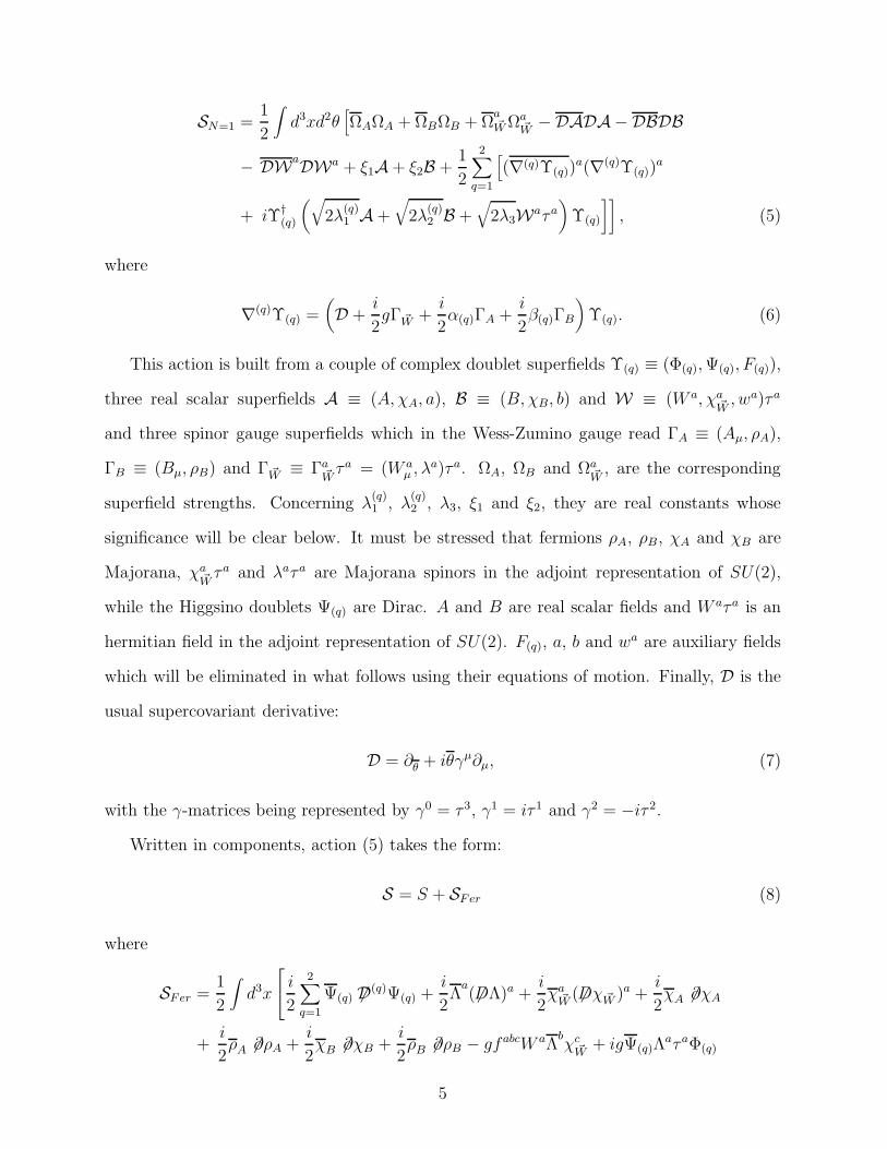
SN=1 =1

2

∫

d3xd2θ[

ΩAΩA + ΩBΩB + Ωa~W Ωa

~W−DADA−DBDB

− DWaDWa + ξ1A + ξ2B +1

2

2∑

q=1

[

(∇(q)Υ(q))a(∇(q)Υ(q))

a

+ iՆ(q)

(√

2λ(q)1 A +

√

2λ(q)2 B +

√

2λ3Waτa

)

Υ(q)

]]

, (5)

where

∇(q)Υ(q) =(

D +i

2gΓ ~W +

i

2α(q)ΓA +

i

2β(q)ΓB

)

Υ(q). (6)

This action is built from a couple of complex doublet superfields Υ(q) ≡ (Φ(q), Ψ(q), F(q)),

three real scalar superfields A ≡ (A, χA, a), B ≡ (B, χB, b) and W ≡ (W a, χa~W, wa)τa

and three spinor gauge superfields which in the Wess-Zumino gauge read ΓA ≡ (Aµ, ρA),

ΓB ≡ (Bµ, ρB) and Γ ~W ≡ Γa~Wτa = (W a

µ , λa)τa. ΩA, ΩB and Ωa~W

, are the corresponding

superfield strengths. Concerning λ(q)1 , λ

(q)2 , λ3, ξ1 and ξ2, they are real constants whose

significance will be clear below. It must be stressed that fermions ρA, ρB, χA and χB are

Majorana, χa~Wτa and λaτa are Majorana spinors in the adjoint representation of SU(2),

while the Higgsino doublets Ψ(q) are Dirac. A and B are real scalar fields and W aτa is an

hermitian field in the adjoint representation of SU(2). F(q), a, b and wa are auxiliary fields

which will be eliminated in what follows using their equations of motion. Finally, D is the

usual supercovariant derivative:

D = ∂θ + iθγµ∂µ, (7)

with the γ-matrices being represented by γ0 = τ 3, γ1 = iτ 1 and γ2 = −iτ 2.

Written in components, action (5) takes the form:

S = S + SFer (8)

where

SFer =1

2

∫

d3x

i

2

2∑

q=1

Ψ(q) 6D(q)Ψ(q) +i

2Λ

a( 6DΛ)a +

i

2χa

~W( 6Dχ ~W )a +

i

2χA 6∂χA

+i

2ρA 6∂ρA +

i

2χB 6∂χB +

i

2ρB 6∂ρB − gfabcW aΛ

bχc

~W+ igΨ(q)Λ

aτaΦ(q)

5

−√

8λ3Ψ(q)χa~WτaΦ(q) + iα(q)Ψ(q)ρAΦ(q) −

√

8λ(q)1 Ψ(q)χAΦ(q)

+ iβ(q)Ψ(q)ρBΦ(q) −√

8λ(q)2 Ψ(q)χBΦ(q)

−2∑

q=1

(

Ψ(q)(√

2λ(q)1 A +

√

2λ(q)2 B +

√

2λ3Waτa)Ψ(q)

)

+ h.c.

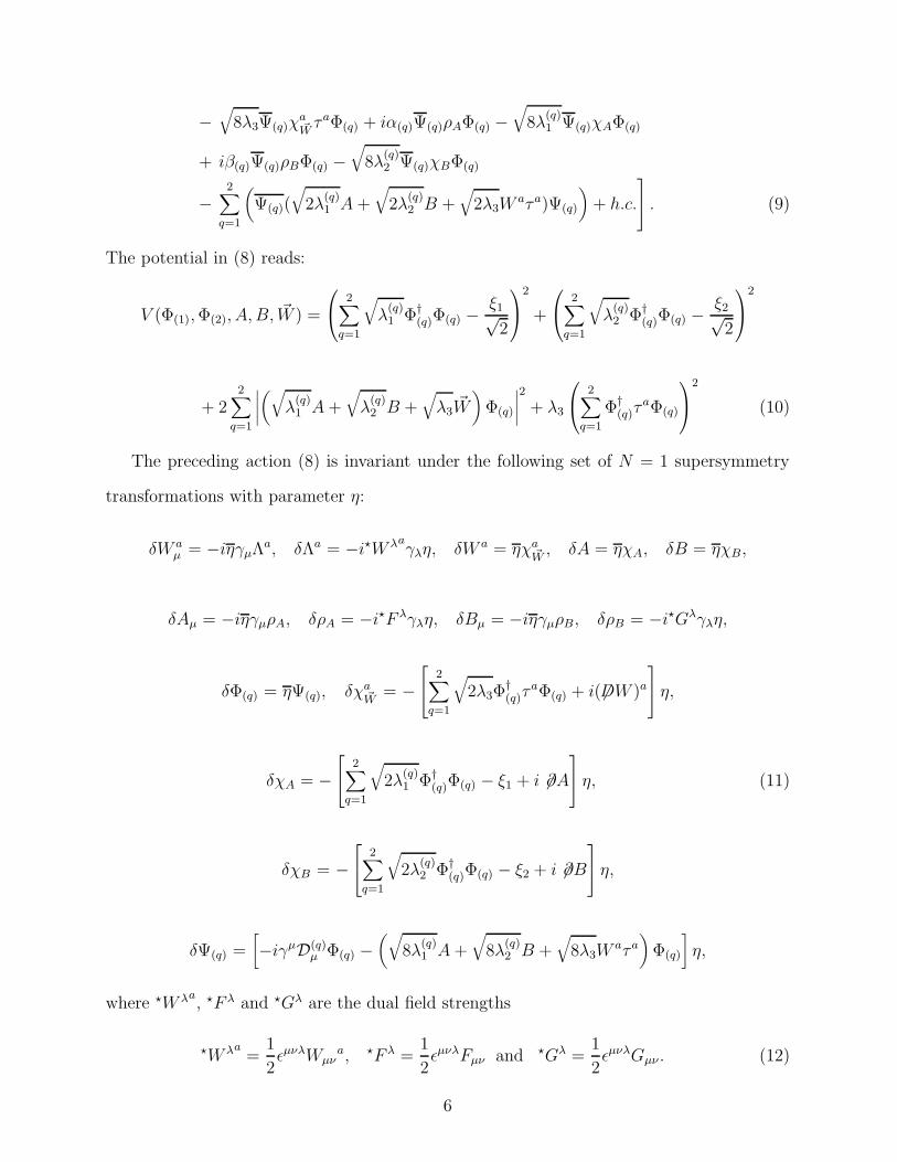
. (9)

The potential in (8) reads:

V (Φ(1), Φ(2), A, B, ~W ) =

2∑

q=1

√

λ(q)1 Φ†

(q)Φ(q) −ξ1√2

2

+

2∑

q=1

√

λ(q)2 Φ†

(q)Φ(q) −ξ2√2

2

+ 22∑

q=1

∣

∣

∣

∣

(√

λ(q)1 A +

√

λ(q)2 B +

√

λ3~W

)

Φ(q)

∣

∣

∣

∣

2

+ λ3

2∑

q=1

Φ†(q)τ

aΦ(q)

2

(10)

The preceding action (8) is invariant under the following set of N = 1 supersymmetry

transformations with parameter η:

δW aµ = −iηγµΛ

a, δΛa = −i⋆W λaγλη, δW a = ηχa

~W, δA = ηχA, δB = ηχB,

δAµ = −iηγµρA, δρA = −i⋆F λγλη, δBµ = −iηγµρB, δρB = −i⋆Gλγλη,

δΦ(q) = ηΨ(q), δχa~W

= −

2∑

q=1

√

2λ3Φ†(q)τ

aΦ(q) + i( 6DW )a

η,

δχA = −

2∑

q=1

√

2λ(q)1 Φ†

(q)Φ(q) − ξ1 + i 6∂A

η, (11)

δχB = −

2∑

q=1

√

2λ(q)2 Φ†

(q)Φ(q) − ξ2 + i 6∂B

η,

δΨ(q) =[

−iγµD(q)µ Φ(q) −

(√

8λ(q)1 A +

√

8λ(q)2 B +

√

8λ3Waτa

)

Φ(q)

]

η,

where ⋆W λa, ⋆F λ and ⋆Gλ are the dual field strengths

⋆W λa=

1

2ǫµνλWµν

a, ⋆F λ =1

2ǫµνλFµν and ⋆Gλ =

1

2ǫµνλGµν . (12)

6

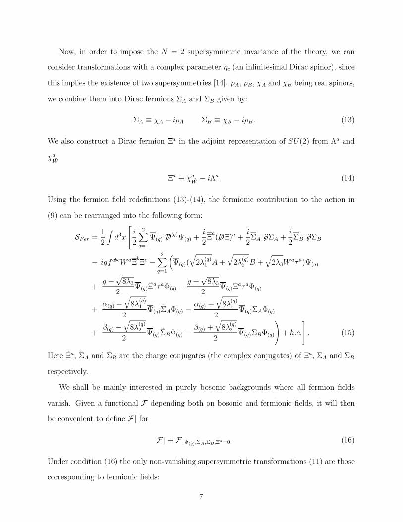
Now, in order to impose the N = 2 supersymmetric invariance of the theory, we can

consider transformations with a complex parameter ηc (an infinitesimal Dirac spinor), since

this implies the existence of two supersymmetries [14]. ρA, ρB, χA and χB being real spinors,

we combine them into Dirac fermions ΣA and ΣB given by:

ΣA ≡ χA − iρA ΣB ≡ χB − iρB. (13)

We also construct a Dirac fermion Ξa in the adjoint representation of SU(2) from Λa and

χa~W

Ξa ≡ χa~W− iΛa. (14)

Using the fermion field redefinitions (13)-(14), the fermionic contribution to the action in

(9) can be rearranged into the following form:

SFer =1

2

∫

d3x

i

2

2∑

q=1

Ψ(q) 6D(q)Ψ(q) +i

2Ξ

a( 6DΞ)a +

i

2ΣA 6∂ΣA +

i

2ΣB 6∂ΣB

− igfabcW aΞbΞc −

2∑

q=1

(

Ψ(q)(√

2λ(q)1 A +

√

2λ(q)2 B +

√

2λ3Waτa)Ψ(q)

+g −

√8λ3

2Ψ(q)Ξ

aτaΦ(q) −g +

√8λ3

2Ψ(q)Ξ

aτaΦ(q)

+α(q) −

√

8λ(q)1

2Ψ(q)ΣAΦ(q) −

α(q) +√

8λ(q)1

2Ψ(q)ΣAΦ(q)

+β(q) −

√

8λ(q)2

2Ψ(q)ΣBΦ(q) −

β(q) +√

8λ(q)2

2Ψ(q)ΣBΦ(q)

+ h.c.

. (15)

Here Ξa, ΣA and ΣB are the charge conjugates (the complex conjugates) of Ξa, ΣA and ΣB

respectively.

We shall be mainly interested in purely bosonic backgrounds where all fermion fields

vanish. Given a functional F depending both on bosonic and fermionic fields, it will then

be convenient to define F| for

F| ≡ F|Ψ(q),ΣA,ΣB,Ξa=0. (16)

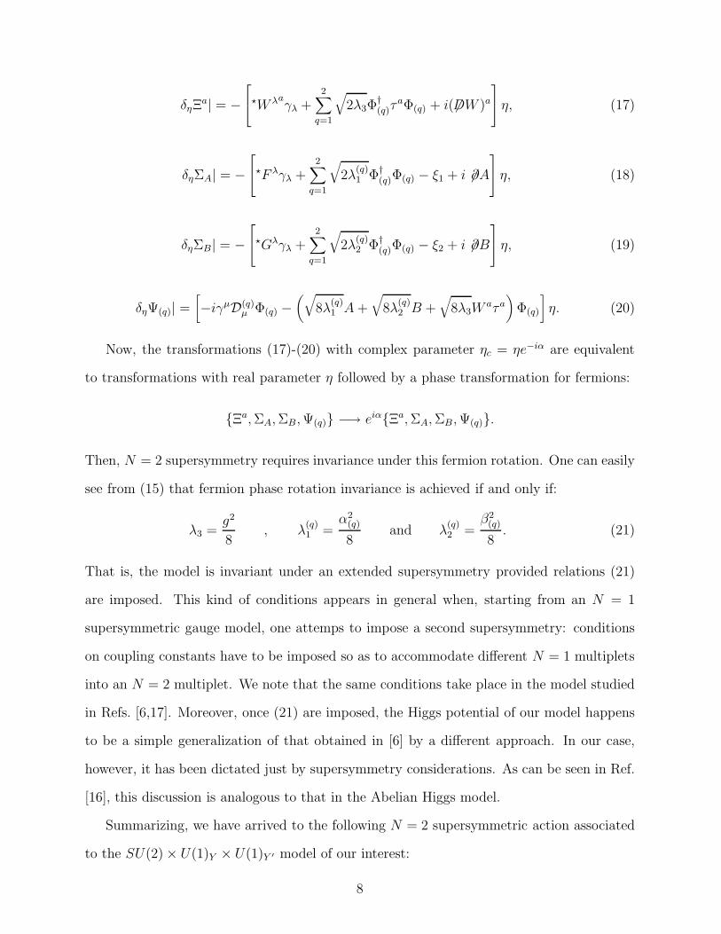
Under condition (16) the only non-vanishing supersymmetric transformations (11) are those

corresponding to fermionic fields:

7

δηΞa| = −

⋆W λaγλ +

2∑

q=1

√

2λ3Φ†(q)τ

aΦ(q) + i( 6DW )a

η, (17)

δηΣA| = −

⋆F λγλ +2∑

q=1

√

2λ(q)1 Φ†

(q)Φ(q) − ξ1 + i 6∂A

η, (18)

δηΣB| = −

⋆Gλγλ +2∑

q=1

√

2λ(q)2 Φ†

(q)Φ(q) − ξ2 + i 6∂B

η, (19)

δηΨ(q)| =[

−iγµD(q)µ Φ(q) −

(√

8λ(q)1 A +

√

8λ(q)2 B +

√

8λ3Waτa

)

Φ(q)

]

η. (20)

Now, the transformations (17)-(20) with complex parameter ηc = ηe−iα are equivalent

to transformations with real parameter η followed by a phase transformation for fermions:

Ξa, ΣA, ΣB, Ψ(q) −→ eiαΞa, ΣA, ΣB, Ψ(q).

Then, N = 2 supersymmetry requires invariance under this fermion rotation. One can easily

see from (15) that fermion phase rotation invariance is achieved if and only if:

λ3 =g2

8, λ

(q)1 =

α2(q)

8and λ

(q)2 =

β2(q)

8. (21)

That is, the model is invariant under an extended supersymmetry provided relations (21)

are imposed. This kind of conditions appears in general when, starting from an N = 1

supersymmetric gauge model, one attemps to impose a second supersymmetry: conditions

on coupling constants have to be imposed so as to accommodate different N = 1 multiplets

into an N = 2 multiplet. We note that the same conditions take place in the model studied

in Refs. [6,17]. Moreover, once (21) are imposed, the Higgs potential of our model happens

to be a simple generalization of that obtained in [6] by a different approach. In our case,

however, it has been dictated just by supersymmetry considerations. As can be seen in Ref.

[16], this discussion is analogous to that in the Abelian Higgs model.

Summarizing, we have arrived to the following N = 2 supersymmetric action associated

to the SU(2) × U(1)Y × U(1)Y ′ model of our interest:

8

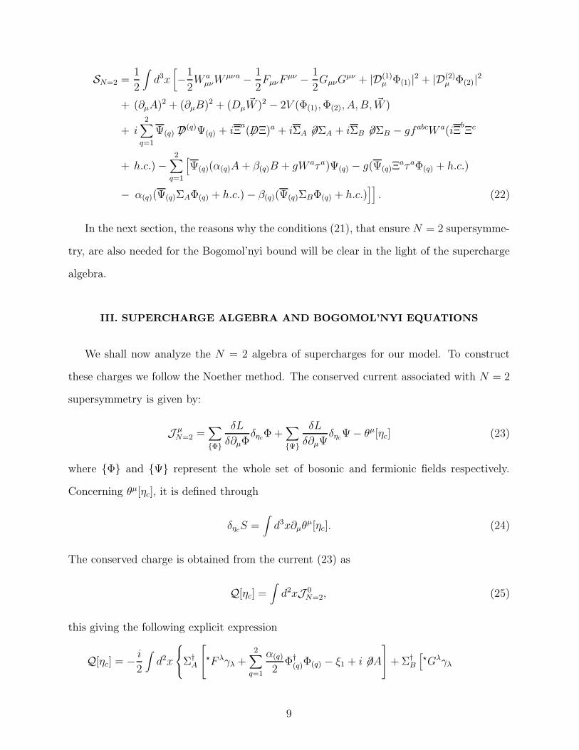
SN=2 =1

2

∫

d3x

[

−1

2W a

µνWµνa − 1

2FµνF

µν − 1

2GµνG

µν + |D(1)µ Φ(1)|2 + |D(2)

µ Φ(2)|2

+ (∂µA)2 + (∂µB)2 + (Dµ~W )2 − 2V (Φ(1), Φ(2), A, B, ~W )

+ i2∑

q=1

Ψ(q) 6D(q)Ψ(q) + iΞa( 6DΞ)a + iΣA 6∂ΣA + iΣB 6∂ΣB − gfabcW a(iΞ

bΞc

+ h.c.) −2∑

q=1

[

Ψ(q)(α(q)A + β(q)B + gW aτa)Ψ(q) − g(Ψ(q)ΞaτaΦ(q) + h.c.)

− α(q)(Ψ(q)ΣAΦ(q) + h.c.) − β(q)(Ψ(q)ΣBΦ(q) + h.c.)]]

. (22)

In the next section, the reasons why the conditions (21), that ensure N = 2 supersymme-

try, are also needed for the Bogomol’nyi bound will be clear in the light of the supercharge

algebra.

III. SUPERCHARGE ALGEBRA AND BOGOMOL’NYI EQUATIONS

We shall now analyze the N = 2 algebra of supercharges for our model. To construct

these charges we follow the Noether method. The conserved current associated with N = 2

supersymmetry is given by:

J µN=2 =

∑

Φ

δL

δ∂µΦδηc

Φ +∑

Ψ

δL

δ∂µΨδηc

Ψ − θµ[ηc] (23)

where Φ and Ψ represent the whole set of bosonic and fermionic fields respectively.

Concerning θµ[ηc], it is defined through

δηcS =

∫

d3x∂µθµ[ηc]. (24)

The conserved charge is obtained from the current (23) as

Q[ηc] =∫

d2xJ 0N=2, (25)

this giving the following explicit expression

Q[ηc] = − i

2

∫

d2x

Σ†A

⋆F λγλ +2∑

q=1

α(q)

2Φ†

(q)Φ(q) − ξ1 + i 6∂A

+ Σ†B

[

⋆Gλγλ

9

+2∑

q=1

β(q)

2Φ†

(q)Φ(q) − ξ2 + i 6∂B

+ Ξ†a

⋆W λaγλ +

g

2

2∑

q=1

Φ†(q)τ

aΦ(q) + i( 6DW )a

+2∑

q=1

Ψ†(q)

[

−iγµD(q)µ Φ(q) −

(

α(q)A + β(q)B + gW aτa)

Φ(q)

]

ηc. (26)

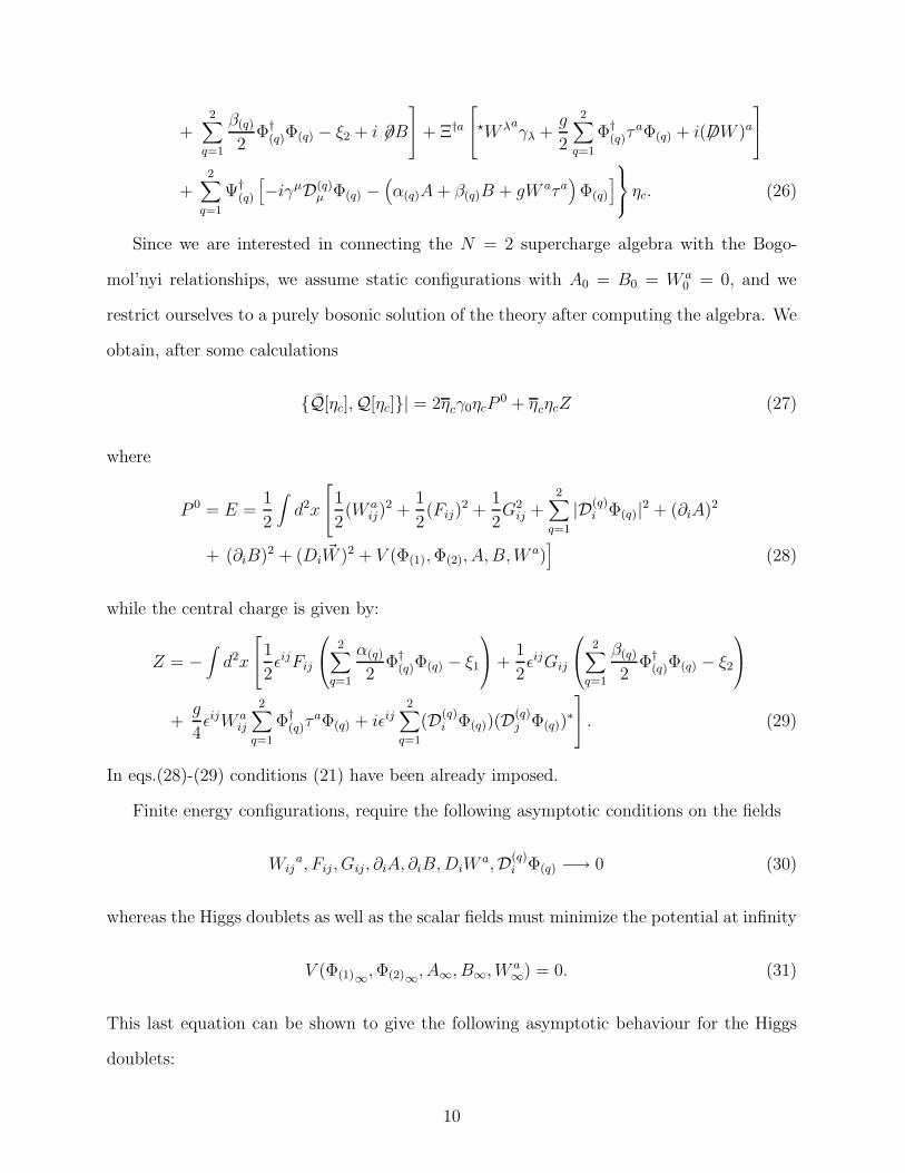
Since we are interested in connecting the N = 2 supercharge algebra with the Bogo-

mol’nyi relationships, we assume static configurations with A0 = B0 = W a0 = 0, and we

restrict ourselves to a purely bosonic solution of the theory after computing the algebra. We

obtain, after some calculations

Q[ηc],Q[ηc]| = 2ηcγ0ηcP0 + ηcηcZ (27)

where

P 0 = E =1

2

∫

d2x

1

2(W a

ij)2 +

1

2(Fij)

2 +1

2G2

ij +2∑

q=1

|D(q)i Φ(q)|2 + (∂iA)2

+ (∂iB)2 + (Di~W )2 + V (Φ(1), Φ(2), A, B, W a)

]

(28)

while the central charge is given by:

Z = −∫

d2x

1

2ǫijFij

2∑

q=1

α(q)

2Φ†

(q)Φ(q) − ξ1

+1

2ǫijGij

2∑

q=1

β(q)

2Φ†

(q)Φ(q) − ξ2

+g

4ǫijW a

ij

2∑

q=1

Φ†(q)τ

aΦ(q) + iǫij2∑

q=1

(D(q)i Φ(q))(D(q)

j Φ(q))∗

. (29)

In eqs.(28)-(29) conditions (21) have been already imposed.

Finite energy configurations, require the following asymptotic conditions on the fields

Wija, Fij , Gij, ∂iA, ∂iB, DiW

a,D(q)i Φ(q) −→ 0 (30)

whereas the Higgs doublets as well as the scalar fields must minimize the potential at infinity

V (Φ(1)∞, Φ(2)∞

, A∞, B∞, W a∞) = 0. (31)

This last equation can be shown to give the following asymptotic behaviour for the Higgs

doublets:

10

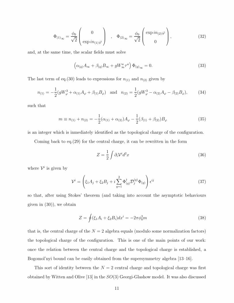
Φ(1)∞=

φ0√2

0

exp in(1)ϕ

, Φ(2)∞=

φ0√2

exp in(2)ϕ

0

, (32)

and, at the same time, the scalar fields must solve

(

α(q)A∞ + β(q)B∞ + gW a∞τa

)

Φ(q)∞= 0. (33)

The last term of eq.(30) leads to expressions for n(1) and n(2) given by

n(1) = −1

2(gW 3

ϕ + α(1)Aϕ + β(1)Bϕ) and n(2) =1

2(gW 3

ϕ − α(2)Aϕ − β(2)Bϕ), (34)

such that

m ≡ n(1) + n(2) = −1

2(α(1) + α(2))Aϕ − 1

2(β(1) + β(2))Bϕ (35)

is an integer which is inmediately identified as the topological charge of the configuration.

Coming back to eq.(29) for the central charge, it can be rewritten in the form

Z =1

2

∫

∂iV id2x (36)

where V i is given by

V i =

ξ1Aj + ξ2Bj + i2∑

q=1

Φ†(q)D

(q)j Φ(q)

ǫij (37)

so that, after using Stokes’ theorem (and taking into account the asymptotic behaviours

given in (30)), we obtain

Z =∮

(ξ1Ai + ξ2Bi)dxi = −2πφ20m (38)

that is, the central charge of the N = 2 algebra equals (modulo some normalization factors)

the topological charge of the configuration. This is one of the main points of our work:

once the relation between the central charge and the topological charge is established, a

Bogomol’nyi bound can be easily obtained from the supersymmetry algebra [13–16].

This sort of identity between the N = 2 central charge and topological charge was first

obtained by Witten and Olive [13] in the SO(3) Georgi-Glashow model. It was also discussed

11

for the self-dual Chern-Simons system by Lee, Lee and Weinberg [14]. Hlousek and Spector

[15] have thoroughly analyzed this connection by studying several models where the existence

of an N = 1 supersymmetry and a topological current implies an N = 2 supersymmetry with

its central charge coinciding with the topological charge. More recently, this connection was

established for the Abelian Higgs model [16] where a condition on the coupling constants has

also been shown to be necessarily imposed. This condition is unavoidable both for having

N = 2 supersymmmetry and the Bogomol’nyi equations. Also, in the study of self-dual

Chern-Simons systems, having a topological charge (related to the magnetic flux) and an

N = 1 extension, a condition on the symmetry breaking coupling constant must be imposed

both to achieve N = 2 extended supersymmetry and to obtain the Bogomolnyi equations

[14].

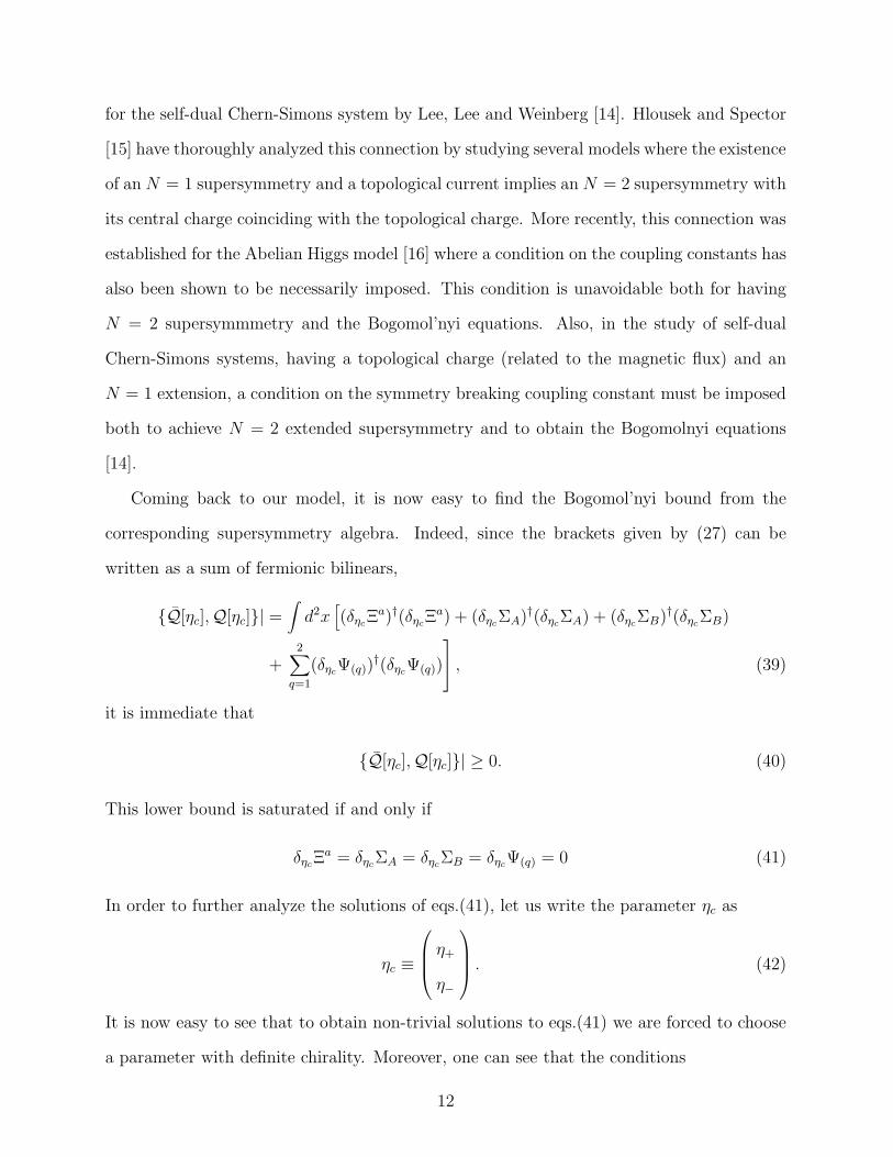
Coming back to our model, it is now easy to find the Bogomol’nyi bound from the

corresponding supersymmetry algebra. Indeed, since the brackets given by (27) can be

written as a sum of fermionic bilinears,

Q[ηc],Q[ηc]| =∫

d2x[

(δηcΞa)†(δηc

Ξa) + (δηcΣA)†(δηc

ΣA) + (δηcΣB)†(δηc

ΣB)

+2∑

q=1

(δηcΨ(q))

†(δηcΨ(q))

, (39)

it is immediate that

Q[ηc],Q[ηc]| ≥ 0. (40)

This lower bound is saturated if and only if

δηcΞa = δηc

ΣA = δηcΣB = δηc

Ψ(q) = 0 (41)

In order to further analyze the solutions of eqs.(41), let us write the parameter ηc as

ηc ≡

η+

η−

. (42)

It is now easy to see that to obtain non-trivial solutions to eqs.(41) we are forced to choose

a parameter with definite chirality. Moreover, one can see that the conditions

12

δη+Ξa = δη+ΣA = δη+ΣB = δη+Ψ(q) = 0 (43)

imply δη−Ξa 6= 0, δη−ΣA 6= 0, δη−ΣB 6= 0, δη−Ψ(q) 6= 0 for nontrivial solutions. Hence if one

is to look for Bogomol’nyi equations corresponding to non-trivial configurations, it makes

sense to consider that ηc has just one independent chiral component, say

ηc ≡

η+

0

. (44)

Let us note, at this point, that for a parameter of this form, the supercharge algebra can be

seen to be

Q[η+],Q[η+]| = η†+η+(2P 0 + Z) (45)

with Z the central charge whose explicit value is given in eq.(38). Then, the inequality (40)

is nothing but the Bogomol’nyi bound of our model

M ≥ πφ20m. (46)

Consequently, eqs.(41) are the Bogomol’nyi equations of the theory (once we identify the

supersymmetry parameter with η+). Explicitly:

ǫijWija + g

2∑

q=1

Φ†(q)τ

aΦ(q) = 0 , (DiW − iǫijDjW )a = 0, (47)

1

2ǫijFij +

2∑

q=1

α(q)

2Φ†

(q)Φ(q) − ξ1 = 0 , (∂i − iǫij∂j)A = 0, (48)

1

2ǫijGij +

2∑

q=1

β(q)

2Φ†

(q)Φ(q) − ξ2 = 0 , (∂i − iǫij∂j)B = 0, (49)

(D(q)i − iǫijD(q)

j )Φ(q) = 0 ,(

α(q)A + β(q)B + gW aτa)

Φ(q) = 0. (50)

Owing to (46), their solutions also solve the static Euler-Lagrange equations of motion.

Let us remark on the fact that field configurations solving the Bogomol’nyi equations

break half of the supersymmetries, a feature common to all models presenting Bogomol’nyi

13

bounds with supersymmetric extension (See for example [17] and References therein). In-

deed, as was seen above, supersymmetry transformations generated by the antichiral param-

eter η− are broken. If we attempt to keep all the supersymmetries of our model, we will find

that the resulting field configuration has zero energy (the trivial vacuum) as easily seen from

eqs.(41). Had we been faced with an antichiral parameter in (44), we would have obtained

antisoliton solutions with a breaking of the supersymmetry transformation generated by η+.

Analogous results also hold in 4 dimensional models as the one originally studied by Witten

and Olive [13].

A careful analysis of the whole set of Bogomol’nyi equations, shows that it is possible to

decouple an equation involving only the Higgs doublet in the same vein as it was previously

done in the abelian Higgs model [12].

IV. LIMITING CASES

As a by-product of our systematic approach, we can easily obtain Bogomol’nyi bounds

(coming from an underlying N = 2 supersymmetric structure) for a variety of models which

have recently acquired physical interest.

A. The SU(2) × U(1)Y × U(1)Y ′ pure-Higgs model

The dynamics of this model first considered in Ref. [6], is dictated by the following

Lagrangian density:

LpH = −1

4~Wµν · ~W µν − 1

4FµνF

µν − 1

4GµνG

µν +1

2

2∑

q=1

|D(q)µ Φ(q)|2 − λ3

2∑

q=1

Φ†(q)τ

aΦ(q)

2

−

2∑

q=1

√

λ(q)1 Φ†

(q)Φ(q) −ξ1√2

2

−

2∑

q=1

√

λ(q)2 Φ†

(q)Φ(q) −ξ2√2

2

. (51)

It is immediately seen that the results given in Ref. [6] can be obtained just by considering

bosonic configurations satisfying the constraint:

A = B = W a = 0. (52)

14

in our equations1. These conditions are consistent with the asymptotic behaviours (30)-(31)

and with the Bogomol’nyi equations (47)-(50) of our model. It is interesting to note that

conditions (21), imposed by the requirement of extended supersymmetry, also fix in this case

the coupling constants exactly as they appear in the above mentioned Reference. Thus, we

have shown that the potential and the coupling constants of the SU(2)×U(1)Y ×U(1)Y ′ pure

Higgs model studied in [6], are simply dictated by N = 2 supersymmetry. A simple ansatz

for string-like solutions of arbitrary topological charge in this system has been explored in

[6]. It is shown there that, interestingly enough, these configurations do not correspond to

an embedding of the Nielsen-Olesen vortex solution.

B. The U(1) × U(1) model

It is well-known that superconducting cosmic strings could have appeared as topological

defects in the early Universe, owing to the presence of a charged field condensate in the core

of the string [18]. Considering that supersymmetry could also have been realized in the early

Universe, the study of supersymmetric models possibly involving superconducting cosmic

strings seems to be relevant. As the superconducting string models are commonly based on

a U(1)×U(1) gauge symmetry [10,18], we will investigate the following Lagrangian density:

LSCS = −1

4FµνF

µν − 1

4GµνG

µν +1

2(D(A)

µ φ)∗(Dµ(A)φ) +1

2(D(B)

µ ξ)∗(Dµ(B)ξ) − V (φ, ξ) (53)

- which can be obtained as a limiting case of our SU(2)×U(1)Y ×U(1)Y ′ system -, where χ

and ξ are abelian (complex) Higgs fields, while D(A)µ and D(B)

µ are the covariant derivatives

with respect to Aµ and Bµ respectively. To this end, we will restrict ourselves to those

solutions of our model satisfying condition (52), which are decoupled from the non-abelian

gauge field W aµ . That is, we are interested in topological classical field configurations in the

1Note that our algebraic approach is not modified by any constraint imposed on purely bosonic

configurations, as all the fermion fields are put to zero after computing the algebra.

15

region of the parameter space where g → 0. We then ask for solutions where the disconnected

non-Abelian field strength is constrained to vanish,

W aµν = 0. (54)

Now, we rename the abelian coupling constants α(1) and β(2),

α(1) = β(2) ≡ e, (55)

and consider the case where the remaining α(2) and β(1) vanish. Finally, we make the

following ansatz for the Higgs sector:

Φ(1) =

φ

0

and Φ(2) =

0

ξ

. (56)

After all these steps, our effective Lagrangian looks exactly as (53), and the explicit form

of the Higgs potential reads:

V (φ, ξ) =e2

8(|φ|2 − v2

1)2 +

e2

8(|ξ|2 − v2

2)2. (57)

Unfortunately, the region of the parameter space spanned by our Higgs coupling constants,

lies outside the range where several interesting phenomena take place (See, for example, Refs.

[9,10]). To study these, we would need to modify our starting-point potential. Nevertheless,

let us mention an interesting result that can be extracted in the model described above. If

we consider the possibility that both U(1) symmetries be broken roughly at the same scale,

finite energy leads to the following asymptotic behaviour for the Higgs fields:

φ → v1einY θ and ξ → v2e

inY ′θ, (58)

where nY and nY ′ are integers that characterize the topological sector to which the solution

belongs. Then, in view of eqs.(36) and (37), it is immediately clear that the central charge

of the corresponding N = 2 supersymmetric theory becomes:

Z = −2πv21

(

nY +v22

v21

nY ′

)

. (59)

16

Thus, the Bogomol’nyi bound of the U(1) × U(1) model presented above is

M ≥ πv21

(

nY +v22

v21

nY ′

)

. (60)

Remarkably, the bound is not directly proportional to the topological charge m = nY +nY ′. It

would be interesting to investigate how this behaviour matches onto the model-independent

approach carried out in Ref. [15].

C. The SU(2)global × U(1)local semi-local model

Finally, it is also interesting to explore how N = 2 supersymmetry guarantees the ex-

istence of a Bogomol’nyi bound for the neutral semi-local string defects with SU(2)global ×

U(1)local symmetry discussed in Ref. [19], even though the vacuum manifold is simply con-

nected. The Lagrangian density of this model takes the following form:

LSL = −1

4FµνF

µν +1

2[(∂µ − ieAµ)Φ]†[(∂µ − ieAµ)Φ] − λ(Φ†Φ − v2)2, (61)

where Φ is a Higgs doublet charged only under the abelian subgroup U(1)local. The potential

is minimum when Φ†Φ = v2. Since Φ is a complex doublet, the minimum of the potential is

a three-sphere and is simply connected. This is in contrast with the situation in the abelian

Higgs model where the potential minimum is a circle and a vortex solution correpond to a

configuration which winds around the circle. However, it was explicitely shown in Ref. [19]

that this model admits of stable string solutions by a simple generalization of Bogomol’nyi’s

proof. We can reproduce their proof as a particular case of our model. In fact, it is easy

to see that imposing conditions (52) and (54), and working in the parameter space region

where g, β(q) → 0, we just have to restrict ourselves to those configurations satisfying the

following constraint:

Φ(2) = Gµν = 0. (62)

Then, the Bogomol’nyi bound obtained in [19] can be easily reproduced following the same

steps as above.

17

Let us end our paper remarking that we have considered an SU(2)×U(1)Y ×U(1)Y ′ gauge

model with a symmetry breaking potential, which can be seen to be a simple extension of the

Electroweak Standard model. The requirement of N = 2 supersymmetry forces a relation

between coupling constants and at the same time, through its supercharge algebra, imposes

the Bogomol’nyi equations on certain classical field configurations. The connection of our

model with realistic supersymmetric extensions of the Standard model, and the possible

existence of string-like solutions in its coupling to supergravity, remain open problems. We

hope to report on these issues in a forthcoming work.

ACKNOWLEDGEMENTS

This work was partially supported by CONICET, Argentina. We would like to thank

F. Schaposnik for a critical reading of the manuscript. J.D.E. is pleased to thank the

Departament d’Estructura i Constituents de la Materia for its kind hospitality.

18

REFERENCES

[1] G.G. Ross, Grand Unified Theories, Frontiers in Physics Vol.60, The Benjamin-

Cummings Publishing Company (1984).

[2] Particle Data Book, Phys. Rev. D50 (1994) 1173.

[3] See for example P. Nath, R. Arnowitt and A.H. Chamseddine, Applied N = 1 Supergrav-

ity, ICTP Series on Theoretical Physics, vol.1, World Scientific (1984) and References

therein.

[4] G.Dvali and G.Senjanovich, Phys. Rev. Lett. 71 (1993) 2376; L. Perivolaropoulos, Phys.

Lett. B316 (1993) 528; M.A. Earnshaw and M. James, Phys. Rev. D48 (1993) 5818;

T.N. Tomaras, Search for solitons in two-Higgs extensions of the Standard Model, Pro-

ceedings of the Conference “Topics in Quantum Field Theory: Modern Methods in

Fundamental Physics”, Maynooth, Ireland, May 1995. Ed. D.H. Tchrakian, World Sci-

entific (1995); C. Bachas and T.N. Tomaras, Phys. Rev. Lett. 76 (1996) 356.

[5] M. Goodband and M. Hindmarsh, Phys. Lett. B370 (1996) 29.

[6] G. Bimonte and G. Lozano, Phys. Lett. B326 (1994) 270.

[7] H.B. Nielsen and P. Olesen, Nucl. Phys. B61 (1973) 45.

[8] P. Peter, Phys. Rev. D49 (1994) 5052; A-C. Davies and P. Peter, Phys. Lett. B358

(1995) 197.

[9] R. Rohm and I. Dasgupta, Phys. Rev. D53 (1996) 1827.

[10] J.R. Morris, Phys. Rev. D53 (1996) 2078;

[11] E.B. Bogomol’nyi, Sov. Jour. Nucl. Phys. 24 (1976) 449.

[12] H. de Vega and F. Schaposnik, Phys. Rev. D14 (1976) 1100.

[13] E. Witten and D. Olive, Phys. Lett. 78B (1978) 97.

19

[14] C. Lee, K. Lee and E.J. Weinberg, Phys. Lett. B243 (1990) 105.

[15] Z. Hlousek and D. Spector, Nucl. Phys. B370 (1992) 143; B397 (1993) 173; Phys. Lett.

B283 (1992) 75; Mod. Phys. Lett. A7 (1992) 3403.

[16] J.D. Edelstein, C. Nunez and F.A. Schaposnik, Phys. Lett. B329 (1994) 39.

[17] J.D. Edelstein, C. Nunez and F.A. Schaposnik, Nucl. Phys. B458 (1996) 165.

[18] E. Witten, Nucl. Phys. B249 (1985) 557.

[19] T. Vachaspati and A. Achucarro, Phys. Rev. D44 (1991) 3067.

20