J. Vis. Commun. Image R. 20 (2009) 478–490

Contents lists available at ScienceDirect

J. Vis. Commun. Image R.

journal homepage: www.elsevier .com/ locate / jvc i

Surface Function Actives

Qi Duan a,c,*, Elsa D. Angelini b, Andrew F. Laine a

a Department of Biomedical Engineering, Columbia University, ET-351, 1210 Amsterdam Avenue, New York, NY 10027, USAb Department of Image and Signal Processing, Ecole Nationale Supérieure des Télécommunications, LTCI, CNRS-UMR 5141, Francec Center for Biomedical Imaging, NYU School of Medicine, 660 1st Ave., FL1, New York, NY 10016, USA

a r t i c l e i n f o a b s t r a c t

Article history:Received 12 October 2007Accepted 8 June 2009Available online 13 June 2009

Keywords:Surface Function ActivesImage segmentationDeformable modelReal-time segmentationVariational approachInterface representation

1047-3203/$ - see front matter � 2009 Elsevier Inc. Adoi:10.1016/j.jvcir.2009.06.002

* Corresponding author. Address: Center for BiomeMedicine, 660 1st Ave., FL1, New York, NY 10016, US

E-mail address: Qi.Duan@nyumc.org (Q. Duan).

Deformable models have been widely used in image segmentation since the introduction of the snakes.Later the introduction of level set frameworks to solve the energy minimization problem associated withthe deformable model overcame some limitations of the parametric active contours with respect to topo-logical changes by embedding surface representations into higher dimensional functions. However, thismay also bring in more computational load so that recent advances in spatio-temporal resolutions of 3D/4D imaging raised some challenges for real-time segmentation, especially for interventional imaging. Inthis context, a novel segmentation framework, Surface Function Actives (SFA), is proposed for real-timesegmentation purpose. SFA has great advantages in terms of potential efficiency, based on its dimension-ality reduction for the surface representation. Utilizing implicit representations with variational frame-work also provides flexibility and benefits currently shared by level set frameworks. An application forminimally-invasive intervention is shown to illustrate the potential applications of this framework.

� 2009 Elsevier Inc. All rights reserved.

1. Introduction

Image segmentation is a critical step for quantitative imageanalysis. In medical imaging, image segmentation is the prerequi-site for quantitative evaluation of morphologies and pathologies.For example, in cardiac imaging, delineating borders of chambersof the heart and valves are of clinical importance to quantify car-diac function. Segmentation of the left ventricular endocardiumis required for quantitative evaluation of the LV function, such asejection fraction or 3D fractional shortening [1]. With recent ad-vances in 3D and 4D imaging techniques towards real-time imag-ing, the amount of data is becoming prohibitively overwhelming.Manual tracing of these large data sets is tedious and impracticalin clinical setting.

In this context, automated or semi-automated segmentationmethods have been proposed and applied to medical image analy-sis to leverage the human efforts involved in the segmentationtask. Based on the mathematical foundation of each method, seg-mentation approaches can be roughly divided into several classes:classification (e.g. thresholding, k-means), region growing (such asfuzzy connectedness [2]), deformable models (e.g. snake [3], levelset [4–7]), active shape [8] and active appearance models [9],and stochastic methods (Markov random field [10], graph cut[11]). Hybrid methods [12] combining different existing methodswere also proposed. Among segmentation methods, deformable

ll rights reserved.

dical Imaging, NYU School ofA. Fax: +1 212 854 5995.

models are still widely used in medical image analysis, especiallyfor cardiac imaging.

The first deformable model parametric formulation was pro-posed by Kass et al. in 1987 [3]. The idea was to digitize the objectboundary into a set of points with predefined connectivity amongthe node; the contour then deforms under the combination ofinternal forces (such as elasticity and inertia) and external forces(such as image gradient force) to align with the desired object’sboundaries. Parametric deformable models, also called snakes in2D, have been widely applied in various segmentation tasks [13].In 1998, Xu et al. [14] proposed the Gradient Vector Flow or GVFas a novel driving force for the snakes. This newly designed forceovercame several drawbacks from the original snake frameworkand increased the performance of the active contour. However,there were still some limitations related to the parametric formu-lation of active contours, such as difficulties to adapt the contour totopological changes, especially in 3D.

In the late 1990s, Sethian et al. [15] proposed a new frameworkcalled level set to overcome these limitations. The basic idea was toembed the contour evolution into iso-value curves of a functionwith higher dimensionality. Such functions were called level setfunctions. Topological changes could be naturally handled withoutadditional efforts. Moreover, highly convoluted surfaces, whichwere very hard to handle for parametric deformable models, couldalso be easily represented. For this reason, level set formulationshave become a research focus in image segmentation in recentyears. In 2001, Chan and Vese [16] introduced their ‘‘active contourwithout edges” approach. In their framework, no image gradientinformation was needed as with traditional deformable models.

Q. Duan et al. / J. Vis. Commun. Image R. 20 (2009) 478–490 479

Instead, driving forces were derived via energy minimization of theMumford–Shah segmentation functional [17] for piecewise-con-stant regions. Their method could easily deal with noisy images.And as a result, this framework has been widely used in ultrasoundsegmentation [18], brain segmentation [19], and many other appli-cations. However, the introduction of level set functions implicitlyincreased the number of parameters of the surface model, whichincreases the demand for computational power. Although manyoptimization modifications such as narrowbanding [20] or fastmarching schemes were proposed, generally speaking, level setframework is still a relatively ‘‘slow” approach especially for 3Dor 4D data.

As imaging technology evolves, demands for real-time feedbackalso increases, mostly for interventional imaging and minimum-invasive surgery. Latest 3D and 4D imaging techniques and real-time imaging techniques not only provide better appreciations ofthe anatomy and function of the body, but also raise a challengefor image segmentation in terms of computational efficiency. Inthis context, a new framework called Surface Function Actives(or SFA) is proposed in this paper to push the limits of real-timesegmentation.

2. Mathematical models

2.1. Interface representation

‘‘Deformable model” is composed of two critical parts: the‘‘model” or the surface representation, which represents the inter-face, and the ‘‘deformation scheme” driven by applied forces,which fits the model to the image for desired segmentation results.In all deformable model methods, interface representation is fun-damental since the interface or boundary is the target object thatneeds to be fitted to the image information to find the desiredboundaries. Mathematically, there are two ways to represent theinterface:

1. Explicit representation: that is representing the surface byexplicitly listing the coordinates of the boundary points (i.e.a parametric representation). This is the representation thatoriginal snakes [21] used. The coordinate system can useeither natural basis or other basis as well, depending onapplications;

2. Implicit representation: that is representing the surface byembedding the boundary as the iso-value curves of some func-tion f called the representation function. Level set functions [4–7]are a good example to embed the interface as the zero level setof a distance function.

-2 -1 0 1 2-2

-1

0

1

2

x

y

--2

0

2

-2

-10

12

y

Φ(x

,y)

)b( )a(

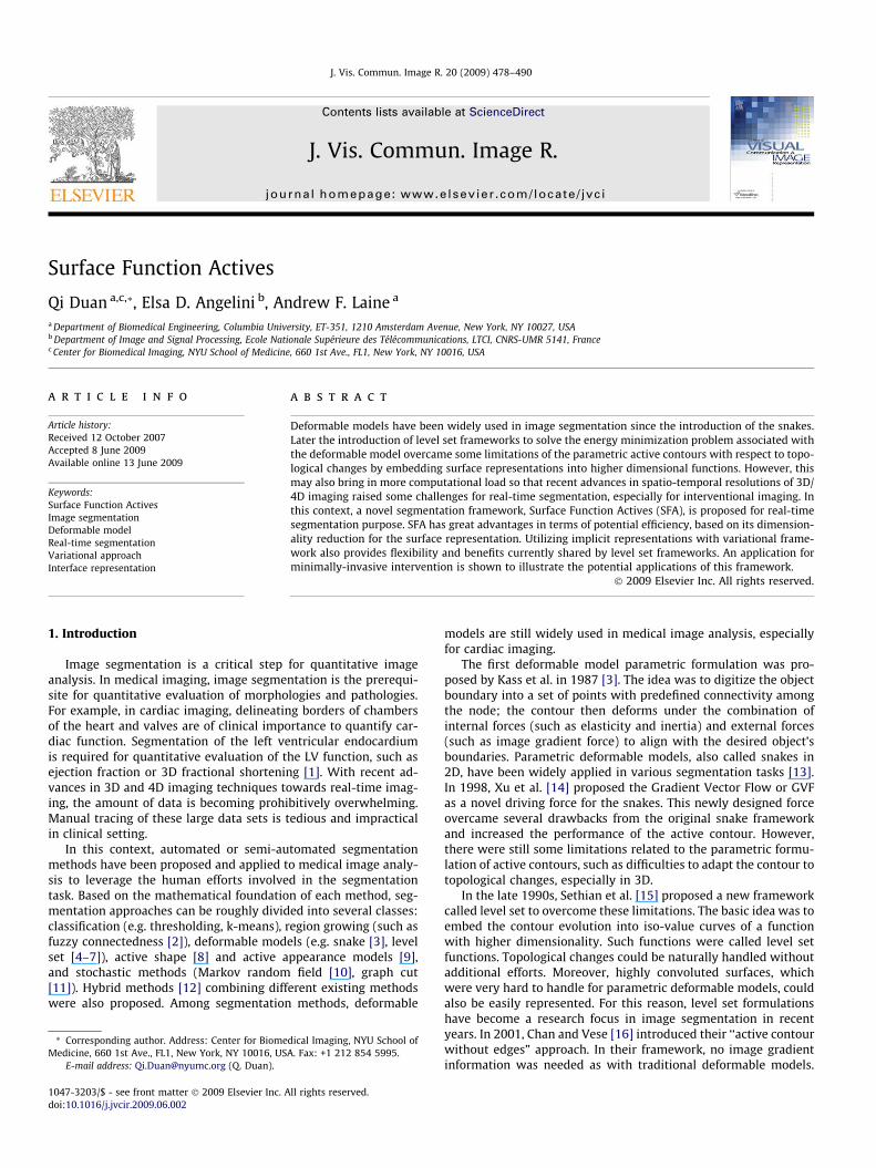
Fig. 1. Illustration of interface representation by three difference frameworks: (a) expliciset; and (c) surface function.

2.2. Surface functions

Most of the recent efforts in segmentation based on implicitinterface representation were focused on the level set framework,given its advantages for topological changes and feasibility to rep-resent convoluted surfaces. As mentioned above, level set func-tions add one extra dimension beyond the dimensionality of theimage data. For example, to represent a surface in 3D space, the le-vel set function corresponding to the surface will be 4D. For com-parison, original parametric deformable models only required a listof point coordinates in 3D. For level set, this extra dimensionbrings various benefits as well as additional computation load,which may degrade computational efficiency.

By looking the opposite way of level set frameworks, it is verynatural to think of dimensionality reduction in surface representa-tion to reduce the computational complexity. Using terminology ofinterface representation, we are looking for a representation func-tion which has fewer dimensions than the image data, i.e. using a2D function to represent a 3D surface in space. We call such func-tion a surface function.

Mathematically, in N dimensional space, we can define a surfacefunction g : RN�1 ! R as a special set of functions representing oneof the coordinates constrained by the others. Without losing gener-ality, we can assume that this special coordinate is x0 and the othercoordinates are x1 to xN-1. That is:

x0 ¼ gðx1; . . . xN�1Þ ð1Þ

The corresponding representation function f is defined as:

f ¼ x0 � gðx1; . . . xN�1Þ: ð2Þ

So that the corresponding boundary is the zero-value curve of thefunction f, i.e. f ð~XÞ ¼ 0; ~X ¼ ðx0; x1; . . . xN�1Þ.

For example, in 2D to represent a straight line with slope = 1and passing through the origin (0, 0), there can be three differentrepresentations:

1. Explicit representation: such as the list of points f. . . ð�1;�1Þ;ð0;0Þ; ð1;1Þ; . . .g;

2. Level set: such as the zero level set of Uðx; y; tÞ ¼ 1ffiffi2p ðx� yÞ, note

that U is a signed distance function, and it is defined on thewhole x–y plane instead of just on the boundary;

3. Surface function: such as y = x.

Fig. 1 illustrates each representation. Note that since these threesurface representations encode the same surface, there are somesimilarities between them. The corresponding representation func-tion for the level set framework is f ¼ 1ffiffi

2p ðx� yÞ ¼ 0; the correspond-

ing representation function for surface function representation is

-2 -1 0 1 2-2

-1

0

1

2

x

y

(c)

20

2

x

t representation; (b) level set framework with the black line showing the zero level

480 Q. Duan et al. / J. Vis. Commun. Image R. 20 (2009) 478–490

f = y � x = 0. It is obvious that both functions have the same roots,with the fact that the coordinates used in the explicit representationare digitized version of these roots. And geometrically, these rootsform the surface we are trying to represent: a straight line withslope = 1 and passing through (0, 0). In other words, explicit repre-sentations, level set distance functions, and surface functions arejust three different equivalent forms of the actual interface functionf for the targeting surface.

In this example, however, besides similarity and equivalence, itis more interesting to notice their differences: the explicit repre-sentation is a set of coordinates defined on the 2D x–y plane; thelevel set function is an R2 ! R distance function defined on thewhole 2D x–y plane; the surface function is an R! R function de-fined only on a 1D x-axis. As a 1D function, surface function repre-sentation has the advantage in efficiency compared with the othertwo common representations. From the example, we can see thatinterface representation based on surface function has less dimen-sionality than both other methods; compared with explicit repre-sentation, surface function can utilize function expression orfunction basis to efficiently represent the interface. Given the factthat most anatomical surfaces are smooth [22], anatomical sur-faces can be efficiently and accurately represented by the surfacefunction framework, which simplifies the downstream mathemat-ical computation such as energy minimizations during imagesegmentation.

2.3. Driving forces

Similar to other deformable models, we adopted a variationalframework in deriving the driving forces. For example, we canuse the Mumford–Shah segmentation energy functional:

Eðf ;~CÞ ¼ bZ

Xðf � gÞ2dV þ a

ZXn~Cjrf j2dV þ c

I~C

ds; ð3Þ

in which~C denotes the smoothed and closed segmented interface, grepresents the observed image data, f is a piecewise smoothedapproximation of g with discontinuities only along~C, and X denotesthe image domain. The first integral enforces similarity between fand g, which is equivalent to homogeneity constraint if f is piece-wise smoothed; the second integral controls the smoothness of f;and the last integral is limits the length of the segmented boundary,which, acts as internal elasticity constraint to prevent leaking atattachment to weak boundaries.

Given the flexibility of variational frameworks, other segmenta-tion energy functionals can be also easily adopted.

In general, deformable models usually utilize iterative methodsto find the optimal solution for the associated energy minimizationframework via curve evolution, which requires an additional vari-able as an artificial time step added into the functions. In this case,curve evolution with explicit representation with K node points be-comes an N � K variable minimization problem since the evolvingcurve is represented by

~X0ðtÞ~X1ðtÞ

..

.

~XK�1ðtÞ

2666664

3777775¼

x00ðtÞ x0

1ðtÞ � � � x0N�1ðtÞ

x10ðtÞ x1

1ðtÞ � � � x1N�1ðtÞ

..

. ... ..

. ...

xK�10 ðtÞ xK�1

1 ðtÞ � � � xK�1N�1ðtÞ

2666664

3777775; ð4Þ

with N � K evolving variables.Curve evolution with level set becomes an (N + 1)-variate func-

tional minimization problem since the evolving curve is repre-sented by

/ð~X; tÞ ¼ /ðx0; x1; . . . xN�1; tÞ; ð5Þ

which has to be solved for every point on the entire image domainor within the narrowband.

Curve evolution with Surface Function Actives becomes an N-variate functional minimization problem since the evolving curvecan be represented by

x0ðtÞ ¼ f ðx1; x2; . . . xN�1; tÞ: ð6Þ

The advantage in dimensionality reduction for Surface Function Ac-tives over level set framework is evident.

The advantage of SFA over explicit expression is in two aspects.First, in explicit representation, for each node point, there are Nevolving variables, whereas in surface function representation,there is only one variable for each corresponding points. This willbecome more evident if we digitize Eq. (6) and reformulate in asimilar form as in Eq. (4):

~X0ðtÞ~X1ðtÞ

..

.

~XK�1ðtÞ

2666664

3777775¼

x00ðtÞ x0

1 � � � x0N�1

x10ðtÞ x1

1 � � � x1N�1

..

. ... ..

. ...

xK�10 ðtÞ xK�1

1 � � � xK�1N�1

2666664

3777775: ð7Þ

Although the memory usage of Eq. (7) is the same as Eq. (4), thecurve evolution of Eq. (7) has N � 1 less dimensionality than Eq.(4), which usually leads to faster and more stable convergence. Gen-erally speaking, the more parameters to be optimized, the largerpossibility that local minimums and saddle points exist, especiallywith presence of noise. Of course it is not necessarily true for everycase that 1D optimization is more stable than N-D; they could beequivalent. But even for that, the searching space for 1D case ismuch smaller than the N-D one, which leads to faster convergence.

Another aspect is that Eq. (6) can be represented via functionbasis, such as cubic Hermite functions, in which case only a fewweighting parameters rather than a lot of digitized node pointshave to be stored and iterated on. This can further improve theaccuracy, efficiency, and numerical stability.

2.4. Comparison with other deformable models

Although as mentioned above, the interface functions for thethree deformable models are equivalent in terms of surface repre-sentation, different ways to approach interface formulation pro-vide different benefits and limitations.

Parametric active contours with explicit representations pro-vide relative simple representations through interface point coor-dinates and do not add additional dimensionality to theoptimization problem. However, it cannot easily handle topologi-cal changes, and usually requires some prior knowledge aboutthe target topology for proper initialization. It is also not trivialto determine whether an arbitrary pixel is inside or outside thesegmented objects. Moreover, in order to compare to other seg-mentation results such as manual tracing, it is usually not veryeasy to directly compute quantitative metrics such as surface dis-tances since it requires pairing of closest points.

The level set framework based on implicit representations viadistance functions can automatically deal with topological changesand allows easy determination of whether a point is inside the ob-ject or not by simply looking at the sign of the level set function atthe point location. However, the level set formulation implicitlyintroduces a new dimension, i.e. the value of the level set function,for each voxel in the whole image data space, whereas the othertwo models only focus on the interface itself. This type of formula-tion implicitly increases the dimensionality of the variational prob-lem and thus increases the computational cost of the optimizationprocess. Even though a narrowband approach can improve the effi-ciency by focusing only around the interface, it still requires more

Q. Duan et al. / J. Vis. Commun. Image R. 20 (2009) 478–490 481

voxel information than the other two formulations. In terms of seg-mentation comparison, if the level set function is the signed dis-tance function, it is very easy to compute the distance betweensurfaces, although in most of implementations, level set functionsafter few iterations do not necessarily remain as signed distancefunctions, especially for those using narrowband approaches.

Surface Function Actives is a kind of marriage of the previouslydiscussed models: it focuses only on the interface as the explicitrepresentation, while being formulated as an implicit representa-tion like the level set framework. It has advantage on dimensional-ity reduction in surface representation compared with level set. Itcan utilize function basis to avoid memory-inefficient boundarypoint digitizing. Even if a digitized form has to be used and the sur-face representation is similar to explicit expression, Surface Func-tion Actives still has faster convergence when compared withparametric deformable model. This dimensionality reduction givesSFA advantages in efficiency in both aspects of the deformablemodel (i.e. surface modeling and deformation scheme). Furthermore, with an implicit representation, it is straightforward todetermine whether a point is inside the contour by simply compar-ing the value of the surface function for that point with the value ofthe surface function on the boundary. In addition, surface functionsenable immediate quantitative evaluation of the segmentation re-sults via surface comparisons and differences in surface functionvalues. However, similar to parametric active contours, it is nottrivial to deal with topological changes.

2.5. Further extension in flexibility

Beside the advantage brought by dimensionality reduction, SFAframework is also benefited from basis representation. By utilizingcoordinate basis other than Cartesian coordinates, SFA can not onlyeasily dealt with enclosed shape as heart, liver and various tumors,but also easily incorporate shape prior information. By utilizingfunction basis other than natural basis, SFA can not only efficientlyrepresent convoluted surfaces, but also naturally enforce priorknowledge on surface smoothness.

By using the concept of piecewise function, SFA can be extendedwith combination of finite element patches to capture much morecomplex shape, like left ventricle. By incorporating repositioningand reorientation, the capture range of SFA can be largely in-creased, giving less dependence on initialization.

A sample application illustrating all these flexibility extensionsin the context of real-time cardiac segmentation was provided la-ter in the paper. But first, some basic idea of SFA was illustrated onsynthetic images using Cartesian coordinate system.

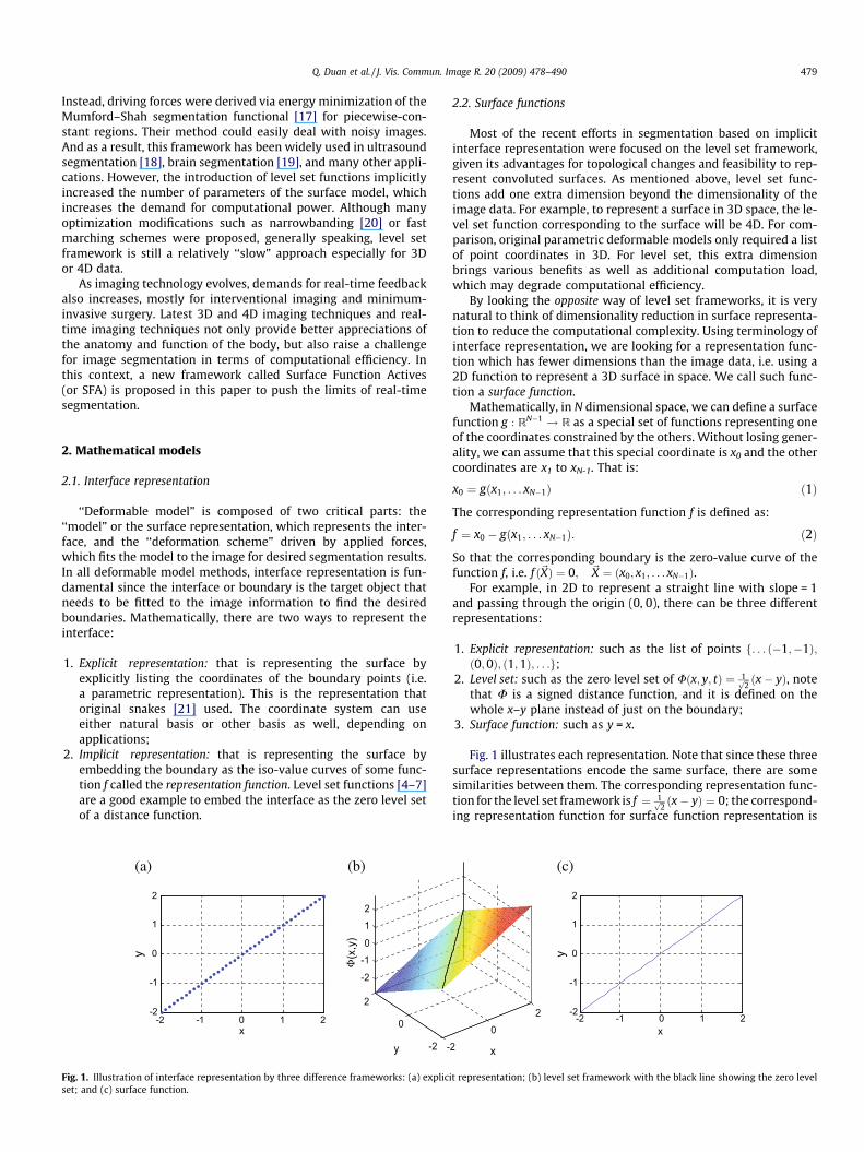
Fig. 2. (a) Synthetic image composed of two regions with normal distributions withthe same mean values but different standard deviations; (b) corresponding binaryimages indicating the ground truth segmentation. The blue region has a standarddeviation of 5 and the red one has a value of 10 in the original image. The interfaceis a sine function.

3. Experimental results on synthetic image

To illustrate the performance and some advantages of the pro-posed Surface Function Actives (SFA), several segmentation exam-ples are presented in this section on a synthetic image. This sectionspecifically focuses on two implicit representation methods: theproposed SFA method and the level set representation. Both seg-mentation frameworks use variational formulae and interfacefunctions. A fair head-to-head comparison is possible by settingidentical segmentation energy functional and numerical schemesfor both methods.

3.1. Synthetic image

To illustrate the flexibility of the proposed SFA framework, in-stead of using an example on common piecewise smooth images,in this section, both SFA and level set approach were challengedwith textured regions segmentation.

The synthetic image, as shown in Fig. 2a, was composed of twoparts. Pixel intensities for each part were randomly sampled fromnormal distributions with identical mean values and differentstandard deviations. The corresponding ground-true binary imageis shown in Fig. 2b. The blue region had a standard deviation of 5and the red region had a value of 10. The interface between the re-gions was a sine function. The dimension of the image was 65 by65 pixels.

3.2. SFA using numerical solution

Usually in image segmentation, especially for the level setframework, it is not easy to find a closed form interface function.Instead, a numerical solution or approximation of the interfacefunction is computed via iterative numerical energy minimization.With the level set functions, this requires computation values ofthe level set function at each pixel (or on a narrowband near theinterface). With SFA, we only need to compute the surface functionvalues at each pixel on the interface.

Given the texture-based segmentation problem presented inFig. 2, the following energy functional was selected:

E¼Z

Xðrðx;yÞ� d1Þ2Hðx;yÞdxdyþ

ZXðrðx;yÞ� d2Þ2ð1�Hðx;yÞÞdxdy

ð8Þ

where X is the image domain, r(x, y) is a standard deviation esti-mator for pixel (x, y) within a small neighborhood, and H is theHeaviside function, which equals 1 inside the current interfaceand 0 outside. The parameters d1 and d2 are computed as the aver-age standard deviations inside and outside the current interface,respectively. The optimal segmentation will partition the imageinto two regions, with relative homogeneous distributions of thestandard deviations within each region. This approach is equivalentto segmenting a representation of local standard deviations r(x, y)values of the image, knowing that for normal distributionsN(l, r), average standard deviations converge to the scale parame-ter r. The Chan-Vese level set numerical schemes described in [6]were used for the level set implementation. For simplification, nocurvature constraints were used.

Both methods were initialized as a straight line at the center ofthe image, as shown in Fig. 3a. The ground truth boundary isshown in green on the same figure. Corresponding surface func-tions for SFA was just a 1D constant function as y(x) = 0,�32 6 x 6 32, whereas the corresponding level set function was aplane with slope 1 as shown in Fig. 3b.

)b( )a(

-200

20

-200

20

-20

0

20

xy

Φ(x

,y)

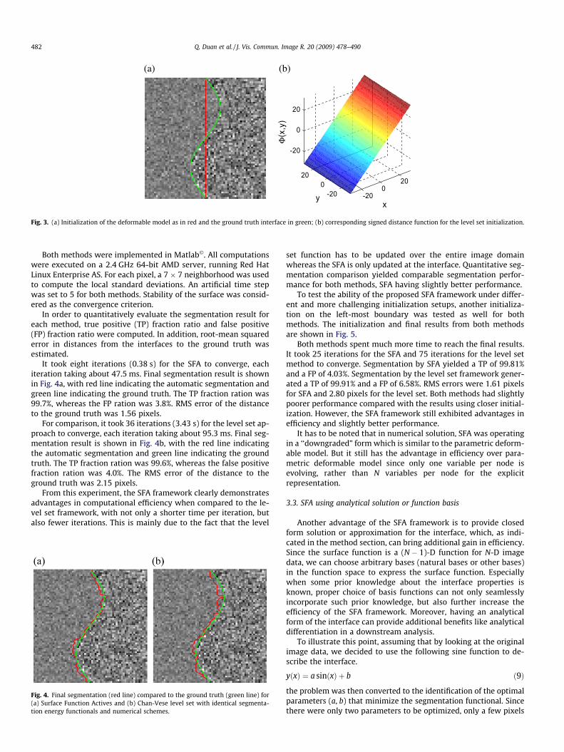
Fig. 3. (a) Initialization of the deformable model as in red and the ground truth interface in green; (b) corresponding signed distance function for the level set initialization.

482 Q. Duan et al. / J. Vis. Commun. Image R. 20 (2009) 478–490

Both methods were implemented in Matlab�. All computationswere executed on a 2.4 GHz 64-bit AMD server, running Red HatLinux Enterprise AS. For each pixel, a 7 � 7 neighborhood was usedto compute the local standard deviations. An artificial time stepwas set to 5 for both methods. Stability of the surface was consid-ered as the convergence criterion.

In order to quantitatively evaluate the segmentation result foreach method, true positive (TP) fraction ratio and false positive(FP) fraction ratio were computed. In addition, root-mean squarederror in distances from the interfaces to the ground truth wasestimated.

It took eight iterations (0.38 s) for the SFA to converge, eachiteration taking about 47.5 ms. Final segmentation result is shownin Fig. 4a, with red line indicating the automatic segmentation andgreen line indicating the ground truth. The TP fraction ration was99.7%, whereas the FP ration was 3.8%. RMS error of the distanceto the ground truth was 1.56 pixels.

For comparison, it took 36 iterations (3.43 s) for the level set ap-proach to converge, each iteration taking about 95.3 ms. Final seg-mentation result is shown in Fig. 4b, with the red line indicatingthe automatic segmentation and green line indicating the groundtruth. The TP fraction ration was 99.6%, whereas the false positivefraction ration was 4.0%. The RMS error of the distance to theground truth was 2.15 pixels.

From this experiment, the SFA framework clearly demonstratesadvantages in computational efficiency when compared to the le-vel set framework, with not only a shorter time per iteration, butalso fewer iterations. This is mainly due to the fact that the level

Fig. 4. Final segmentation (red line) compared to the ground truth (green line) for(a) Surface Function Actives and (b) Chan-Vese level set with identical segmenta-tion energy functionals and numerical schemes.

set function has to be updated over the entire image domainwhereas the SFA is only updated at the interface. Quantitative seg-mentation comparison yielded comparable segmentation perfor-mance for both methods, SFA having slightly better performance.

To test the ability of the proposed SFA framework under differ-ent and more challenging initialization setups, another initializa-tion on the left-most boundary was tested as well for bothmethods. The initialization and final results from both methodsare shown in Fig. 5.

Both methods spent much more time to reach the final results.It took 25 iterations for the SFA and 75 iterations for the level setmethod to converge. Segmentation by SFA yielded a TP of 99.81%and a FP of 4.03%. Segmentation by the level set framework gener-ated a TP of 99.91% and a FP of 6.58%. RMS errors were 1.61 pixelsfor SFA and 2.80 pixels for the level set. Both methods had slightlypoorer performance compared with the results using closer initial-ization. However, the SFA framework still exhibited advantages inefficiency and slightly better performance.

It has to be noted that in numerical solution, SFA was operatingin a ‘‘downgraded” form which is similar to the parametric deform-able model. But it still has the advantage in efficiency over para-metric deformable model since only one variable per node isevolving, rather than N variables per node for the explicitrepresentation.

3.3. SFA using analytical solution or function basis

Another advantage of the SFA framework is to provide closedform solution or approximation for the interface, which, as indi-cated in the method section, can bring additional gain in efficiency.Since the surface function is a (N � 1)-D function for N-D imagedata, we can choose arbitrary bases (natural bases or other bases)in the function space to express the surface function. Especiallywhen some prior knowledge about the interface properties isknown, proper choice of basis functions can not only seamlesslyincorporate such prior knowledge, but also further increase theefficiency of the SFA framework. Moreover, having an analyticalform of the interface can provide additional benefits like analyticaldifferentiation in a downstream analysis.

To illustrate this point, assuming that by looking at the originalimage data, we decided to use the following sine function to de-scribe the interface.

yðxÞ ¼ a sinðxÞ þ b ð9Þ

the problem was then converted to the identification of the optimalparameters (a, b) that minimize the segmentation functional. Sincethere were only two parameters to be optimized, only a few pixels

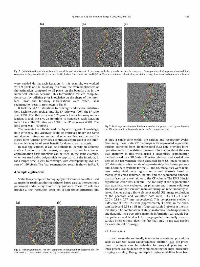
Fig. 5. (a) Initialization of the deformable model, in red, at left-most of the image with the ground-true interface in green; Corresponding final segmentation (red line)compared to the ground truth (green line) for (b) Surface Function Actives and (c) Chan-Vese level set under identical segmentation energy functional and numerical schemes.

Fig. 7. Final segmentation (red line) compared to the ground truth (green line) forthe SFA using cubic polynomials as the surface approximation.

Q. Duan et al. / J. Vis. Commun. Image R. 20 (2009) 478–490 483

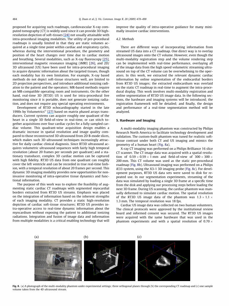
were needed during each iteration. In this example, we workedwith 9 pixels on the boundary to ensure the overcompleteness ofthe estimation, compared to all pixels on the boundary as in thenumerical solution scenario. This formulation reduces computa-tional cost by utilizing prior knowledge on the shape of the inter-face. Close and far-away initializations were tested. Finalsegmentation results are shown in Fig. 6.

It took the SFA 10 iterations to converge under close initializa-tion. Each iteration took 21 ms. The TP ratio was 100%; the FP ratiowas 3.79%. The RMS error was 1.26 pixels. Under far-away initial-ization, it took the SFA 25 iterations to converge. Each iterationtook 17 ms. The TP ratio was 100%; the FP ratio was 4.50%. TheRMS error was 1.40 pixels.

The presented results showed that by utilizing prior knowledge,both efficiency and accuracy could be improved under the sameinitialization setups and numerical schemes. Besides, the use of aclosed form function provides a continuous expression of the inter-face which may be of great benefit for downstream analysis.

In real applications, it can be difficult to identify an accuratesurface function. In this context, an approximation function orapproximation basis functions can be used. In the same example,when we used cubic polynomials to approximate the interface, ittook longer time, 3.59 s, to converge, with corresponding RMS er-rors of 1.66 pixels. The final segmentation result is shown in Fig. 7.

4. Sample applications

Static X-ray computed tomography (CT) volumes are often usedas anatomic roadmaps during catheter-based cardiac interventionsperformed under X-ray fluoroscopy guidance. These CT volumesprovide a high-resolution depiction of soft-tissue structures, but

Fig. 6. Final segmentation (red line) compared to the ground truth (green line) forSFA under (a) close initialization and (b) far-away initialization.

at only a single time within the cardiac and respiratory cycles.Combining these static CT roadmaps with segmented myocardialborders extracted from 4D ultrasound (US) data provides intra-operative access to real-time dynamic information about the car-diac anatomy. In this work, using a customized segmentationmethod based on a 3D Surface Function Actives, endocardial bor-ders of the left ventricle were extracted from US image volumes(4D data sets) at a frame rate of approximately five frames per sec-ond. Coordinate systems for the CT and US modalities were regis-tered using rigid body registration at end diastole based onmanually selected landmark points, and the segmented endocar-dial surfaces were overlaid onto the CT volume. The RMS fiducialregistration error was 3.80 mm. The accuracy of the segmentationwas quantitatively evaluated on phantom and human volunteerstudies via comparison with manual tracings on nine randomly se-lected frames using a finite element model (US image resolutionsof the phantom and volunteer data were 1.3 � 1.1 � 1.3 and0.70 � 0.82 � 0.77 mm, respectively). This comparison yielded aRMS error of 3.70 ± 2.5 mm (approximately 3 pixels) in the phan-tom study and 2.58 ± 1.58 mm (approximately 3 pixels) in the clin-ical study. The combination of static anatomical roadmap volumesand dynamic intra-operative anatomic information can enable bet-ter guidance and feedback for image-guided minimally invasivecardiac interventions, given the fact that only 75 ms was neededfor each clinical 3D image.

4.1. Introduction

In cardiovascular minimally invasive interventional proceduressuch as catheter-based radiofrequency ablation [23], pre-proce-dural roadmaps can be valuable for surgical planning andintra-procedural guidance by complementing the intra-proceduralimaging modality. Though multiple imaging modalities have been

484 Q. Duan et al. / J. Vis. Commun. Image R. 20 (2009) 478–490

proposed for acquiring such roadmaps, cardiovascular X-ray com-puted tomography (CT) is widely used since it can provide 3D high-resolution depiction of soft-tissues [24] not usually attainable withintra-procedural imaging modalities. The utility of pre-proceduralroadmaps is usually limited in that they are static volumes ac-quired at a single time point within cardiac and respiratory cycles,whereas during the interventional procedure, the geometry andposition of the heart changes over time due to cardiac motionand breathing. Several modalities, such as X-ray fluoroscopy [25],interventional magnetic resonance imaging (iMRI) [26], and 2D/3D ultrasound (US) have been used for intra-procedural imagingto acquire dynamic information about the targeted tissues, thougheach modality has its own limitation. For example, X-ray basedmethods do not depict soft-tissue structures well, are limited to2D projection perspectives, and introduce additional ionizing radi-ation to the patient and the operators; MR-based methods requirean MR-compatible operating room and instruments. On the otherhand, real-time 3D (RT3D) US is used for intra-procedural livemonitoring since it is portable, does not generate ionizing radia-tion, and does not require any special operating environments.

Development of RT3D echocardiography started in the late1990s by Volumetrics� [27] based on matrix phased arrays trans-ducers. Current systems can acquire roughly one quadrant of theheart in a single 3D field-of-view in real-time, or can stitch to-gether acquisitions over four cardiac cycles for a fully sampled car-diac volume. This quadrant-wise acquisition design enables adramatic increase in spatial resolution and image quality com-pared to those reconstructed 3D ultrasound from 2D B-mode slices,which makes such 3D ultrasound techniques increasingly attrac-tive for daily cardiac clinical diagnosis. Since RT3D ultrasound ac-quires volumetric ultrasound sequences with fairly high temporalresolution (about 20 frames per seconds per quadrant) and a sta-tionary transducer, complex 3D cardiac motion can be capturedwith high fidelity. RT3D US data from one quadrant can roughlycover the left ventricle and can be recorded in true real-time fash-ion, with a temporal resolution of about 20 frames per second. Thisdynamic 3D imaging modality provides new opportunities for non-invasive monitoring of intra-operative tissue dynamics and func-tional information.

The purpose of this work was to explore the feasibility of aug-menting static cardiac CT roadmaps with segmented myocardialborders extracted from RT3D US streams. Emphasis was placedon the integration of information based on the inherent strengthsof each imaging modality. CT provides a static high-resolutiondepiction of cardiac soft-tissue structures; RT3D US provides in-tra-operative access to real-time dynamic information about themyocardium without exposing the patient to additional ionizingradiations. Integration and fusion of image data and informationfrom multiple modalities is a critical enabling technology that will

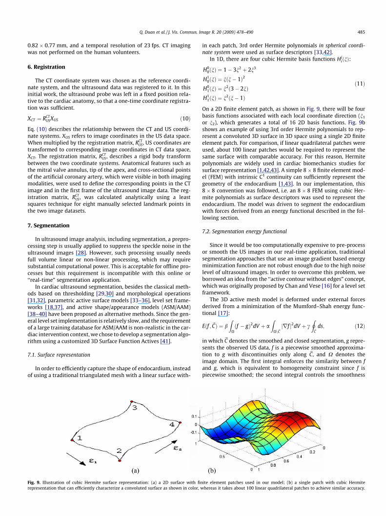
Fig. 8. (a) A photograph of the multi-modality phantom under experimental settings; thrvolume taken from the 4D ultrasound stream.

improve the quality of intra-operative guidance for many mini-mally invasive cardiac interventions.

4.2. Methods

There are different ways of incorporating information fromstreamed US data into a CT roadmap. One direct way is to overlayultrasound images onto the CT volume. However, even though themulti-modality registration step and the volume rendering stepcan be implemented with real-time performance, overlaying allof the image data from the high speed volumetric streaming ultra-sound on top of the CT volume can be overwhelming to the oper-ators. In this work, we extracted the relevant dynamic cardiacinformation by online segmentation of the endocardial bordersfrom RT3D US images; the extracted endocardium was overlaidon the static CT roadmap in real-time to augment the intra-proce-dural display. This work involves multi-modality registration andonline segmentation of RT3D US image data. In the following sec-tions, the hardware and imaging systems will be introduced; theregistration framework will be detailed; and finally, the designand performance of a real-time segmentation method will beanalyzed.

5. Hardware and Imaging

A multi-modality imaging phantom was constructed by PhilipsResearch North America to facilitate technology development andvalidation. The custom-built phantom was tuned for realistic soft-tissue contrast under both CT and US imaging and mimics thegeometry of a human heart (Fig. 8a).

X-ray CT imaging was performed on a Philips Brilliance 16 sliceCT scanner. The CT image data was acquired with a spatial resolu-tion of 0.59 � 0.59 � 1 mm and field-of-view of 300 � 300 �200 mm. This CT volume was used as the static pre-proceduralroadmap (Fig. 8b). Ultrasound imaging was performed on a PhilipsiE33 system, using the X3-1 3D imaging probe (Fig. 8c). For devel-opment purposes, RT3D US data sets were saved to disk for re-peated use. In our segmentation experiments, streaming of thedata was simulated by loading a single 3D frame at a specific timefrom the disk and applying our processing steps before loading thenext 3D frame. During US scanning, the cardiac phantom was man-ually deformed to simulate cardiac motion. The spatial resolutionof the RT3D US image data of the phantom was 1.3 � 1.1 �1.3 mm. The temporal resolution was 18 fps.

Cardiac US image data was collected on two human volunteers.The clinical protocols were approved by the institutional reviewboard and informed consent was secured. The RT3D US imageswere acquired with the same hardware that was used in thephantom experiments and with a spatial resolution of 0.70 �

ee orthogonal planes through (b) the corresponding CT roadmap and (c) one sample

Q. Duan et al. / J. Vis. Commun. Image R. 20 (2009) 478–490 485

0.82 � 0.77 mm, and a temporal resolution of 23 fps. CT imagingwas not performed on the human volunteers.

6. Registration

The CT coordinate system was chosen as the reference coordi-nate system, and the ultrasound data was registered to it. In thisinitial work, the ultrasound probe was left in a fixed position rela-tive to the cardiac anatomy, so that a one-time coordinate registra-tion was sufficient.

XCT ¼ RCTUSXUS ð10Þ

Eq. (10) describes the relationship between the CT and US coordi-nate systems. XUS refers to image coordinates in the US data space.When multiplied by the registration matrix, RCT

US, US coordinates aretransformed to corresponding image coordinates in CT data space,XCT. The registration matrix, RCT

US, describes a rigid body transformbetween the two coordinate systems. Anatomical features such asthe mitral valve annulus, tip of the apex, and cross-sectional pointsof the artificial coronary artery, which were visible in both imagingmodalities, were used to define the corresponding points in the CTimage and in the first frame of the ultrasound image data. The reg-istration matrix, RCT

US, was calculated analytically using a leastsquares technique for eight manually selected landmark points inthe two image datasets.

7. Segmentation

In ultrasound image analysis, including segmentation, a prepro-cessing step is usually applied to suppress the speckle noise in theultrasound images [28]. However, such processing usually needsfull volume linear or non-linear processing, which may requiresubstantial computational power. This is acceptable for offline pro-cesses but this requirement is incompatible with this online or‘‘real-time” segmentation application.

In cardiac ultrasound segmentation, besides the classical meth-ods based on thresholding [29,30] and morphological operations[31,32], parametric active surface models [33–36], level set frame-works [18,37], and active shape/appearance models (ASM/AAM)[38–40] have been proposed as alternative methods. Since the gen-eral level set implementation is relatively slow, and the requirementof a large training database for ASM/AAM is non-realistic in the car-diac intervention context, we chose to develop a segmentation algo-rithm using a customized 3D Surface Function Actives [41].

7.1. Surface representation

In order to efficiently capture the shape of endocardium, insteadof using a traditional triangulated mesh with a linear surface with-

Fig. 9. Illustration of cubic Hermite surface representation: (a) a 2D surface with finrepresentation that can efficiently characterize a convoluted surface as shown in color, w

in each patch, 3rd order Hermite polynomials in spherical coordi-nate system were used as surface descriptors [33,42].

In 1D, there are four cubic Hermite basis functions HjiðnÞ:

H00ðnÞ ¼ 1� 3n2 þ 2n3

H10ðnÞ ¼ nðn� 1Þ2

H01ðnÞ ¼ n2ð3� 2nÞ

H11ðnÞ ¼ n2ðn� 1Þ

ð11Þ

On a 2D finite element patch, as shown in Fig. 9, there will be fourbasis functions associated with each local coordinate direction (n1

or n2), which generates a total of 16 2D basis functions. Fig. 9bshows an example of using 3rd order Hermite polynomials to rep-resent a convoluted 3D surface in 3D space using a single 2D finiteelement patch. For comparison, if linear quadrilateral patches wereused, about 100 linear patches would be required to represent thesame surface with comparable accuracy. For this reason, Hermitepolynomials are widely used in cardiac biomechanics studies forsurface representation [1,42,43]. A simple 8 � 8 finite element mod-el (FEM) with intrinsic C1 continuity can sufficiently represent thegeometry of the endocardium [1,43]. In our implementation, this8 � 8 convention was followed, i.e. an 8 � 8 FEM using cubic Her-mite polynomials as surface descriptors was used to represent theendocardium. The model was driven to segment the endocardiumwith forces derived from an energy functional described in the fol-lowing section.

7.2. Segmentation energy functional

Since it would be too computationally expensive to pre-processor smooth the US images in our real-time application, traditionalsegmentation approaches that use an image gradient based energyminimization function are not robust enough due to the high noiselevel of ultrasound images. In order to overcome this problem, weborrowed an idea from the ‘‘active contour without edges” concept,which was originally proposed by Chan and Vese [16] for a level setframework.

The 3D active mesh model is deformed under external forcesderived from a minimization of the Mumford–Shah energy func-tional [17]:

Eðf ;~CÞ ¼ bZ

Xðf � gÞ2dV þ a

ZXn~Cjrf j2dV þ c

I~C

ds; ð12Þ

in which~C denotes the smoothed and closed segmentation, g repre-sents the observed US data, f is a piecewise smoothed approxima-tion to g with discontinuities only along ~C, and X denotes theimage domain. The first integral enforces the similarity between fand g, which is equivalent to homogeneity constraint since f ispiecewise smoothed; the second integral controls the smoothness

ite element patches used in our model; (b) a single patch with cubic Hermitehereas it takes about 100 linear quadrilateral patches to achieve similar accuracy.

486 Q. Duan et al. / J. Vis. Commun. Image R. 20 (2009) 478–490

of f; and the last integral is actually the length of the segmentedboundary, which, acts as internal elasticity to prevent leaking atweak boundaries. The external forces driving the 3D active meshwere formulated using the same image homogeneity-based ratio-nale proposed by Chan and Vese [16], using homogeneity measuresinside and outside regions based on the current segmentation. Spe-cifically, the optimum segmentation, corresponding to endocar-dium, divides the image into two relatively homogeneous regions.In this application, these regions correspond to the blood pool andthe myocardium.

The Mumford–Shah equation (Eq. (12)) was only evaluated atdiscrete sampled sub-node points. To ensure that the system waswell-defined, each surface patch was super-sampled by a 4 � 4sub-node grid. In this way, the whole surface model was over-con-strained with continuity constraints between each adjacent surfacepatch since the surface basis functions were cubic. The Mumford–Shah equation (Eq. (12)) was minimized using a Newton Downhillmethod, chosen for its computational efficiency

Hi;tþdt ¼ Hi;t � dt@E

@Hi; ð13Þ

with dt representing the artificial time step in numerical iterations.

7.3. Repositioning and reorientation of the surface

One common drawback of segmentation using parametric ac-tive surface models is that the capture range of the method is usu-ally small compared to other methods. For ultrasoundsegmentation applications, the initial contour is usually requiredto be positioned, usually manually, fairly close to the actual bound-ary [13]. Automated and semi-automated methods have been pro-posed to avoid manual intervention, using optical flow tracking[13], the Hough transform [44], or multi-scale approaches [45].Since temporal performance is critically important for our real-time interventional application, a computationally more efficientapproach was needed.

In order to reduce the dependence of the segmentation result onthe initial position, after segmentation convergence for the currentframe, the interface model used for the initialization of the nextframe repositions itself so align its center and long-axis with thecentroid and the long-axis of the segmented surface. This extra stepin the initialization procedure speeds up the convergence, and keepsthe Hermite coefficients at each node as small as possible, which in-creases the numerical stability of the optimization process.

7.4. Implementation

The segmentation software was implemented in C++ using anITK [46]/VTK [47] compatible framework. These open source

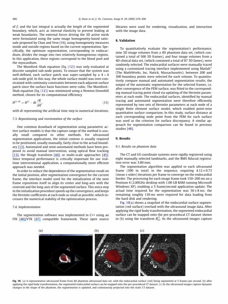
Fig. 10. (a) A representative ultrasound frame from 4D phantom ultrasound data set, wapplying the rigid body transformation, the segmented endocardial surface can be mappechanges in the shape of the phantom, the segmentation is updated, and continuously p

libraries were used for rendering, visualization, and interactionwith the image data.

8. Validation

To quantitatively evaluate the segmentation’s performance,nine 3D image volumes from a 4D phantom data set, (which con-tained a total of 500 3D frames), and four image volumes from a4D clinical data set, (which contained a total of 87 3D fames), wererandomly selected. The endocardial surfaces were manually tracedusing a customized tracing interface implemented using Matlab�

(The MathWorks, Inc, Natick, Massachusetts); between 200 and300 boundary points were selected for each volume. To quantita-tively compare manual and automated segmentation results, theoutput of the automatic segmentation for the selected frames, i.e.after convergence of the FEM surface, was fitted to the correspond-ing manual tracing point cloud via updating of the Hermite param-eters at each node. The endocardial surfaces, identified by manualtracing and automated segmentation were therefore efficientlyrepresented by two sets of Hermite parameters at each node of asingle finite element surface model, which enabled point-wisequantitative surface comparison. In this study, surface distance ateach corresponding node point from the FEM for each surfacewas used as the criterion for surface discrepancy. A similar ap-proach for segmentation comparison can be found in previousstudies [48].

9. Results

9.1. Results on phantom data

The CT and US coordinate systems were rigidly registered usingeight manually selected landmarks, and the RMS fiducial registra-tion error was 3.80 mm.

The segmentation algorithm was applied to each ultrasoundframe (500 in total) in the sequence, requiring 4.12 ± 0.73(mean ± stdev) iterations per frame to converge on the endocardialborder. The processing for each image frame took 150–200 ms on aPentium 4 (2.80GHz desktop with 1.00 GB RAM running MicrosoftWindows XP), enabling a 5 frame/second application update. Theactual time required for the segmentation was 50 ± 8 ms; theremaining roughly 130 ms were required for data loading fromthe hard disk and rendering.

Fig. 10(a) shows a snapshot of the endocardial surface segmen-tation (red surface) overlaid with the ultrasound image data. Afterapplying the rigid body transformation, the segmented endocardialsurface can be mapped onto the pre-procedural CT dataset shownin (b) using the transform RCT

US. As the ultrasound images capture

ith the endocardial surface (red) being segmented at 5 frames per second. (b) afterd onto the pre-procedural CT dataset. (c) As the ultrasound images capture dynamic

rojected into the static CT dataset.

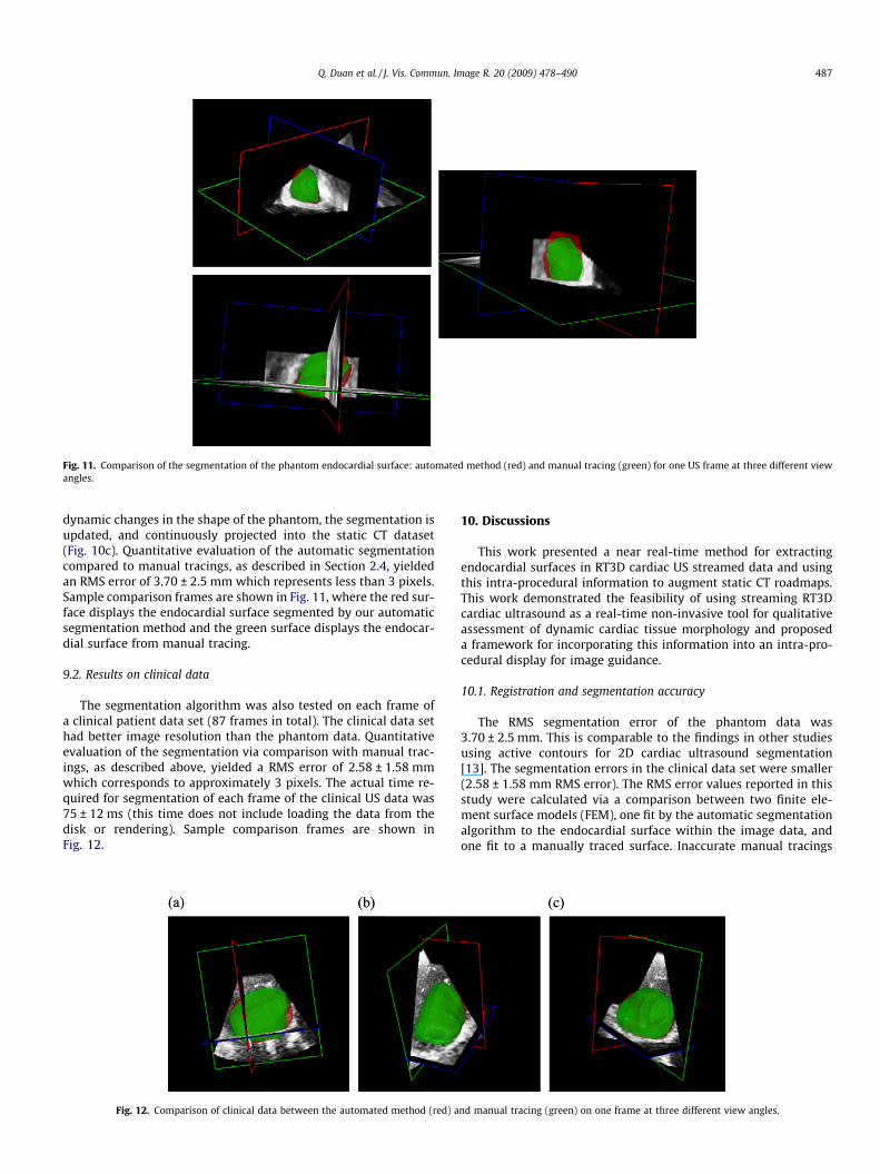
Fig. 11. Comparison of the segmentation of the phantom endocardial surface: automated method (red) and manual tracing (green) for one US frame at three different viewangles.

Q. Duan et al. / J. Vis. Commun. Image R. 20 (2009) 478–490 487

dynamic changes in the shape of the phantom, the segmentation isupdated, and continuously projected into the static CT dataset(Fig. 10c). Quantitative evaluation of the automatic segmentationcompared to manual tracings, as described in Section 2.4, yieldedan RMS error of 3.70 ± 2.5 mm which represents less than 3 pixels.Sample comparison frames are shown in Fig. 11, where the red sur-face displays the endocardial surface segmented by our automaticsegmentation method and the green surface displays the endocar-dial surface from manual tracing.

9.2. Results on clinical data

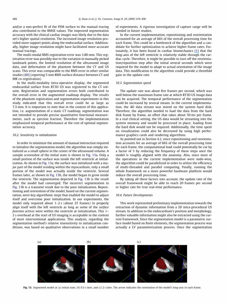
The segmentation algorithm was also tested on each frame ofa clinical patient data set (87 frames in total). The clinical data sethad better image resolution than the phantom data. Quantitativeevaluation of the segmentation via comparison with manual trac-ings, as described above, yielded a RMS error of 2.58 ± 1.58 mmwhich corresponds to approximately 3 pixels. The actual time re-quired for segmentation of each frame of the clinical US data was75 ± 12 ms (this time does not include loading the data from thedisk or rendering). Sample comparison frames are shown inFig. 12.

Fig. 12. Comparison of clinical data between the automated method (red) a

10. Discussions

This work presented a near real-time method for extractingendocardial surfaces in RT3D cardiac US streamed data and usingthis intra-procedural information to augment static CT roadmaps.This work demonstrated the feasibility of using streaming RT3Dcardiac ultrasound as a real-time non-invasive tool for qualitativeassessment of dynamic cardiac tissue morphology and proposeda framework for incorporating this information into an intra-pro-cedural display for image guidance.

10.1. Registration and segmentation accuracy

The RMS segmentation error of the phantom data was3.70 ± 2.5 mm. This is comparable to the findings in other studiesusing active contours for 2D cardiac ultrasound segmentation[13]. The segmentation errors in the clinical data set were smaller(2.58 ± 1.58 mm RMS error). The RMS error values reported in thisstudy were calculated via a comparison between two finite ele-ment surface models (FEM), one fit by the automatic segmentationalgorithm to the endocardial surface within the image data, andone fit to a manually traced surface. Inaccurate manual tracings

nd manual tracing (green) on one frame at three different view angles.

488 Q. Duan et al. / J. Vis. Commun. Image R. 20 (2009) 478–490

and/or a non-perfect fit of the FEM surface to the manual tracingalso contributed to the RMSE values. The improved segmentationaccuracy with the clinical cardiac images was likely due to the dataset’s higher spatial resolution. The increased image resolution pro-vided more support points along the endocardial surface. Addition-ally, higher image resolution might have facilitated more accuratemanual tracings.

The multi-modal RMS registration error was 3.80 mm. This reg-istration error was possibly due to the variation in manually pickedlandmark points, the limited resolution of the ultrasound imagedata, and deformation of the phantom between the CT and USscans. This error was comparable to the RMS error in other similarstudies [49] (reporting 5 mm RMS surface distance between CT andMR co-registration).

In the multi-modality intra-operative display, the segmentedendocardial surface from RT3D US was registered to the CT vol-ume. Registration and segmentation errors both contributed tothe overall error in the augmented roadmap display. The resultsof the phantom registration and segmentation experiments in thisstudy indicated that this overall error could be as large as7.5 mm. It is important to note that in the context of this applica-tion, i.e. augmentation of a static CT roadmap, segmentation wasnot intended to provide precise quantitative functional measure-ments, such as ejection fraction. Therefore the implementationemphasized temporal performance at the cost of optimal segmen-tation accuracy.

10.2. Sensitivity to initialization

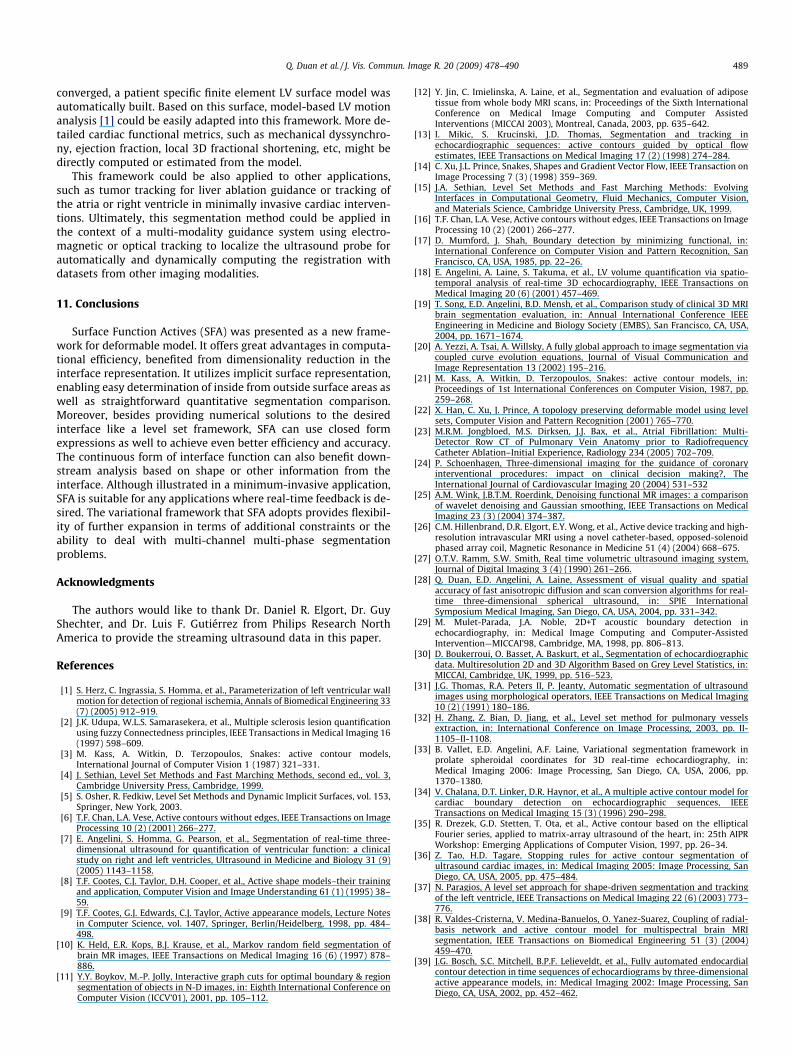
In order to minimize the amount of manual interaction requiredto initialize the segmentation model, the algorithm was simply ini-tialized as a small sphere in the center of the ultrasound volume. Asample screenshot of the initial state is shown in Fig. 13a. Only asmall portion of the surface was inside the left ventricle at initial-ization. As shown in Fig. 13a, the surface was initialized with a ma-jor part of the model residing within the myocardium; only a smallportion of the model was actually inside the ventricle. Severalframes later, as shown in Fig. 13b, the model began to grow insidethe ventricle. The segmentation depicted in Fig. 13b is the resultafter the model had converged. The incorrect segmentation inFig. 13b is a transient result due to the poor initialization. Reposi-tioning and reoriention of the model, based on the current segmen-tation, were key algorithmic steps that enabled the model to adjustitself and overcome poor initialization. In our experiments, themodel only required about 1–2 s (about 25 frames) to properlyalign itself with the left ventricle as long as some of the surfacefunction actives were within the ventricle at initialization. This 1–2 s overhead at the start of US imaging is acceptable in the contextof most interventional applications. This analysis, regarding thesegmentation method’s relative insensitivity to initialization con-ditions, was based on qualitative observations in a small number

Fig. 13. Segmented model at (a) initial state, (b) 0.5 s later, and (c) 2 s later. T

of experiments. A rigorous investigation of capture range will beneeded in future studies.

In the current implementation, repositioning and reorientationaccounted for an average of 66% of the overall processing time foreach frame. This could be a bottleneck of the algorithm and a can-didate for further optimization to achieve higher frame rates. For-tunately, it has been found in cardiac biomechanics [1] that thelong-axis of the left ventricle is relatively stable through the car-diac cycle. Therefore, it might be possible to turn off the reorienta-tion/reposition step after the initial several seconds which wererequired for the model to adapt to actual orientation of the imagedata. This modification to the algorithm could provide a threefoldgain in the update rate.

10.3. Segmentation speed

The update rate was about five frames per second, which waswell below the maximum frame rate at which RT3D US image datacan be acquired. The temporal performance of the segmentationcould be increased by several means. In the current implementa-tion, the 4D data stream was stored on the system hard disk.Therefore, the algorithm needed to load the data from the harddisk frame by frame, an effort that takes about 50 ms per frame.In a real clinical setting, the US data would be streaming into thesystem memory and would be processed in place; loading fromthe hard disk would not be required. Additionally, the time spenton visualization could also be decreased by using high perfor-mance graphics cards and rendering algorithms.

As pointed out in Section 4.2, since repositioning and reorienta-tion accounts for an average of 66% of the overall processing timefor each frame, the computational load could potentially be cut bya factor of 3 by reducing the frequency of these steps once themodel is roughly aligned with the anatomy. Also, since most ofthe operations in the current implementation were node-wise,the algorithm could be parallelized in order to utilize the efficiencyof multi-threaded and parallel computing. Finally, running thewhole framework on a more powerful hardware platform wouldreduce the overall processing time.

By taking all these factors into account, the update rate of theoverall framework might be able to reach 20 frames per secondor higher rate for true real-time performance.

10.4. Future Developments

This work represented preliminary implementation towards theextraction of dynamic information from a 3D intra-procedural USstream. In addition to the endocardium’s position and morphology,further valuable information might also be extracted using the cur-rent framework. Since the segmentation model is a parametric sur-face model based on finite elements, the segmentation process wasactually a LV parameterization process. Once the segmentation

he arrow indicates the orientation of the model’s long-axis in each frame.

Q. Duan et al. / J. Vis. Commun. Image R. 20 (2009) 478–490 489

converged, a patient specific finite element LV surface model wasautomatically built. Based on this surface, model-based LV motionanalysis [1] could be easily adapted into this framework. More de-tailed cardiac functional metrics, such as mechanical dyssynchro-ny, ejection fraction, local 3D fractional shortening, etc, might bedirectly computed or estimated from the model.

This framework could be also applied to other applications,such as tumor tracking for liver ablation guidance or tracking ofthe atria or right ventricle in minimally invasive cardiac interven-tions. Ultimately, this segmentation method could be applied inthe context of a multi-modality guidance system using electro-magnetic or optical tracking to localize the ultrasound probe forautomatically and dynamically computing the registration withdatasets from other imaging modalities.

11. Conclusions

Surface Function Actives (SFA) was presented as a new frame-work for deformable model. It offers great advantages in computa-tional efficiency, benefited from dimensionality reduction in theinterface representation. It utilizes implicit surface representation,enabling easy determination of inside from outside surface areas aswell as straightforward quantitative segmentation comparison.Moreover, besides providing numerical solutions to the desiredinterface like a level set framework, SFA can use closed formexpressions as well to achieve even better efficiency and accuracy.The continuous form of interface function can also benefit down-stream analysis based on shape or other information from theinterface. Although illustrated in a minimum-invasive application,SFA is suitable for any applications where real-time feedback is de-sired. The variational framework that SFA adopts provides flexibil-ity of further expansion in terms of additional constraints or theability to deal with multi-channel multi-phase segmentationproblems.

Acknowledgments

The authors would like to thank Dr. Daniel R. Elgort, Dr. GuyShechter, and Dr. Luis F. Gutiérrez from Philips Research NorthAmerica to provide the streaming ultrasound data in this paper.

References

[1] S. Herz, C. Ingrassia, S. Homma, et al., Parameterization of left ventricular wallmotion for detection of regional ischemia, Annals of Biomedical Engineering 33(7) (2005) 912–919.

[2] J.K. Udupa, W.L.S. Samarasekera, et al., Multiple sclerosis lesion quantificationusing fuzzy Connectedness principles, IEEE Transactions in Medical Imaging 16(1997) 598–609.

[3] M. Kass, A. Witkin, D. Terzopoulos, Snakes: active contour models,International Journal of Computer Vision 1 (1987) 321–331.

[4] J. Sethian, Level Set Methods and Fast Marching Methods, second ed., vol. 3,Cambridge University Press, Cambridge, 1999.

[5] S. Osher, R. Fedkiw, Level Set Methods and Dynamic Implicit Surfaces, vol. 153,Springer, New York, 2003.

[6] T.F. Chan, L.A. Vese, Active contours without edges, IEEE Transactions on ImageProcessing 10 (2) (2001) 266–277.

[7] E. Angelini, S. Homma, G. Pearson, et al., Segmentation of real-time three-dimensional ultrasound for quantification of ventricular function: a clinicalstudy on right and left ventricles, Ultrasound in Medicine and Biology 31 (9)(2005) 1143–1158.

[8] T.F. Cootes, C.J. Taylor, D.H. Cooper, et al., Active shape models–their trainingand application, Computer Vision and Image Understanding 61 (1) (1995) 38–59.

[9] T.F. Cootes, G.J. Edwards, C.J. Taylor, Active appearance models, Lecture Notesin Computer Science, vol. 1407, Springer, Berlin/Heidelberg, 1998, pp. 484–498.

[10] K. Held, E.R. Kops, B.J. Krause, et al., Markov random field segmentation ofbrain MR images, IEEE Transactions on Medical Imaging 16 (6) (1997) 878–886.

[11] Y.Y. Boykov, M.-P. Jolly, Interactive graph cuts for optimal boundary & regionsegmentation of objects in N-D images, in: Eighth International Conference onComputer Vision (ICCV’01), 2001, pp. 105–112.

[12] Y. Jin, C. Imielinska, A. Laine, et al., Segmentation and evaluation of adiposetissue from whole body MRI scans, in: Proceedings of the Sixth InternationalConference on Medical Image Computing and Computer AssistedInterventions (MICCAI 2003), Montreal, Canada, 2003, pp. 635–642.

[13] I. Mikic, S. Krucinski, J.D. Thomas, Segmentation and tracking inechocardiographic sequences: active contours guided by optical flowestimates, IEEE Transactions on Medical Imaging 17 (2) (1998) 274–284.

[14] C. Xu, J.L. Prince, Snakes, Shapes and Gradient Vector Flow, IEEE Transaction onImage Processing 7 (3) (1998) 359–369.

[15] J.A. Sethian, Level Set Methods and Fast Marching Methods: EvolvingInterfaces in Computational Geometry, Fluid Mechanics, Computer Vision,and Materials Science, Cambridge University Press, Cambridge, UK, 1999.

[16] T.F. Chan, L.A. Vese, Active contours without edges, IEEE Transactions on ImageProcessing 10 (2) (2001) 266–277.

[17] D. Mumford, J. Shah, Boundary detection by minimizing functional, in:International Conference on Computer Vision and Pattern Recognition, SanFrancisco, CA, USA, 1985, pp. 22–26.

[18] E. Angelini, A. Laine, S. Takuma, et al., LV volume quantification via spatio-temporal analysis of real-time 3D echocardiography, IEEE Transactions onMedical Imaging 20 (6) (2001) 457–469.

[19] T. Song, E.D. Angelini, B.D. Mensh, et al., Comparison study of clinical 3D MRIbrain segmentation evaluation, in: Annual International Conference IEEEEngineering in Medicine and Biology Society (EMBS), San Francisco, CA, USA,2004, pp. 1671–1674.

[20] A. Yezzi, A. Tsai, A. Willsky, A fully global approach to image segmentation viacoupled curve evolution equations, Journal of Visual Communication andImage Representation 13 (2002) 195–216.

[21] M. Kass, A. Witkin, D. Terzopoulos, Snakes: active contour models, in:Proceedings of 1st International Conferences on Computer Vision, 1987, pp.259–268.

[22] X. Han, C. Xu, J. Prince, A topology preserving deformable model using levelsets, Computer Vision and Pattern Recognition (2001) 765–770.

[23] M.R.M. Jongbloed, M.S. Dirksen, J.J. Bax, et al., Atrial Fibrillation: Multi-Detector Row CT of Pulmonary Vein Anatomy prior to RadiofrequencyCatheter Ablation–Initial Experience, Radiology 234 (2005) 702–709.

[24] P. Schoenhagen, Three-dimensional imaging for the guidance of coronaryinterventional procedures: impact on clinical decision making?, TheInternational Journal of Cardiovascular Imaging 20 (2004) 531–532

[25] A.M. Wink, J.B.T.M. Roerdink, Denoising functional MR images: a comparisonof wavelet denoising and Gaussian smoothing, IEEE Transactions on MedicalImaging 23 (3) (2004) 374–387.

[26] C.M. Hillenbrand, D.R. Elgort, E.Y. Wong, et al., Active device tracking and high-resolution intravascular MRI using a novel catheter-based, opposed-solenoidphased array coil, Magnetic Resonance in Medicine 51 (4) (2004) 668–675.

[27] O.T.V. Ramm, S.W. Smith, Real time volumetric ultrasound imaging system,Journal of Digital Imaging 3 (4) (1990) 261–266.

[28] Q. Duan, E.D. Angelini, A. Laine, Assessment of visual quality and spatialaccuracy of fast anisotropic diffusion and scan conversion algorithms for real-time three-dimensional spherical ultrasound, in: SPIE InternationalSymposium Medical Imaging, San Diego, CA, USA, 2004, pp. 331–342.

[29] M. Mulet-Parada, J.A. Noble, 2D+T acoustic boundary detection inechocardiography, in: Medical Image Computing and Computer-AssistedIntervention—MICCAI’98, Cambridge, MA, 1998, pp. 806–813.

[30] D. Boukerroui, O. Basset, A. Baskurt, et al., Segmentation of echocardiographicdata. Multiresolution 2D and 3D Algorithm Based on Grey Level Statistics, in:MICCAI, Cambridge, UK, 1999, pp. 516–523.

[31] J.G. Thomas, R.A. Peters II, P. Jeanty, Automatic segmentation of ultrasoundimages using morphological operators, IEEE Transactions on Medical Imaging10 (2) (1991) 180–186.

[32] H. Zhang, Z. Bian, D. Jiang, et al., Level set method for pulmonary vesselsextraction, in: International Conference on Image Processing, 2003, pp. II-1105–II-1108.

[33] B. Vallet, E.D. Angelini, A.F. Laine, Variational segmentation framework inprolate spheroidal coordinates for 3D real-time echocardiography, in:Medical Imaging 2006: Image Processing, San Diego, CA, USA, 2006, pp.1370–1380.

[34] V. Chalana, D.T. Linker, D.R. Haynor, et al., A multiple active contour model forcardiac boundary detection on echocardiographic sequences, IEEETransactions on Medical Imaging 15 (3) (1996) 290–298.

[35] R. Drezek, G.D. Stetten, T. Ota, et al., Active contour based on the ellipticalFourier series, applied to matrix-array ultrasound of the heart, in: 25th AIPRWorkshop: Emerging Applications of Computer Vision, 1997, pp. 26–34.

[36] Z. Tao, H.D. Tagare, Stopping rules for active contour segmentation ofultrasound cardiac images, in: Medical Imaging 2005: Image Processing, SanDiego, CA, USA, 2005, pp. 475–484.

[37] N. Paragios, A level set approach for shape-driven segmentation and trackingof the left ventricle, IEEE Transactions on Medical Imaging 22 (6) (2003) 773–776.

[38] R. Valdes-Cristerna, V. Medina-Banuelos, O. Yanez-Suarez, Coupling of radial-basis network and active contour model for multispectral brain MRIsegmentation, IEEE Transactions on Biomedical Engineering 51 (3) (2004)459–470.

[39] J.G. Bosch, S.C. Mitchell, B.P.F. Lelieveldt, et al., Fully automated endocardialcontour detection in time sequences of echocardiograms by three-dimensionalactive appearance models, in: Medical Imaging 2002: Image Processing, SanDiego, CA, USA, 2002, pp. 452–462.

490 Q. Duan et al. / J. Vis. Commun. Image R. 20 (2009) 478–490

[40] S.C. Mitchell, J.G. Bosch, B.P.F. Lelieveldt, et al., 3-D active appearance models:segmentation of cardiac MR and ultrasound images, IEEE Transactions onMedical Imaging 21 (9) (2002) 1167–1178.

[41] B. Vallet, E. Angelini, A. Laine, Variational segmentation framework in prolatespheroidal coordinates for 3D real-time echocardiography, in: SPIE MedicalImaging Conference, San Diego, CA, USA, 2006, pp. 61444A.1–61444A.11.

[42] G.R. Christie, D.P. Bullivant, S.A. Blackett, et al., Modelling and visualising theheart, Computing and Visualization in Science 4 (4) (2004) 227–235.

[43] P.M. Nielsen, I.J. LeGrice, B.H. Smaill, et al., Mathematical model of geometryand fibrous structure of the heart, American Journal of Physiology—Heart andCirculation Physiology 260 (1991) H1365–H1378.

[44] T. Wang, I.Y.H. Gu, M. Viberg, et al., Tracking moving objects in video usingenhanced mean shift and region-based motion field, in: EUSIPCO, 2007, pp.307–311.

[45] J. Chung, P. Abraszewski, X. Yu, et al., Paradoxical increase in ventriculartorsion and systolic torsion rate in type I diabetic patients under tight

glycemic control, Journal of the American College of Cardiology 47 (2)(2006) 384–390.

[46] P. Hellier, C. Barillot, I. Corouge, et al., Retrospective evaluation of intersubjectbrain registration, IEEE Transaction on Medical Imaging 22 (9) (2003) 1120–1130.

[47] E.D. Angelini, T. Song, B.D. Mensh, et al., Segmentation and quantitativeevaluation of brain MRI data with a multi-phase three-dimensional implicitdeformable mode, in: SPIE International Symposium, Medical Imaging 2004,San Diego, CA, USA, 2004, pp. 526–537.

[48] Q. Duan, E. D. Angelini, S. L. Herz, et al., Tracking of LV endocardial surface onreal-time three-dimensional ultrasound with optical flow, in: ThirdInternational Conference on Functional Imaging and Modeling of the Heart2005, Barcelona, Spain, 2005, pp. 434–445.

[49] T. O’Donnell, S. Aharon, S.S. Halliburton, et al., Multi-modality model-basedregistration in the cardiac domain, in: IEEE Conference on Computer Visionand Pattern Recognition, 2000, pp. 790–791.