Systematic bias of Tibetan Plateau snow cover in subseasonal

1

Systematic bias of Tibetan Plateau snow cover in subseasonal-to-seasonal models Shuzhen Hu1, Wenkai Li1 1Key Laboratory of Meteorological Disaster, Ministry of Education (KLME)/Joint International Research Laboratory of Climate and Environment Change (ILCEC)/Collaborative Innovation Center on Forecast and Evaluation of Meteorological 5 Disasters (CIC-FEMD), Nanjing University of Information Science & Technology, Nanjing, 210044, China

Correspondence to: Wenkai Li ([email protected])

Abstract. Accurate subseasonal-to-seasonal (S2S) atmospheric forecasts and hydrological forecasts have considerable

socioeconomic value. This study conducts a multimodel comparison of the Tibetan Plateau snow cover (TPSC) prediction skill

using three models (ECMWF, NCEP and CMA) selected from the S2S project database to understand their performance in 10

capturing TPSC variability. S2S models can skilfully forecast TPSC within a lead time of 2 weeks but show limited skill

beyond 3 weeks. Compared with the observational snow cover analysis, all three models tend to overestimate the area of TPSC,

especially during winter. Another remarkable issue regarding the TPSC forecast is the increasing TPSC with forecast lead time,

which further increases the systematic positive biases of TPSC in the S2S models at longer forecast lead times. The

underestimation of TPSC dissipation induces an increase in TPSC with forecast lead time in the models. Such systematic 15

biases of TPSC influence the forecasted surface air temperature in the S2S models. The surface air temperature over the Tibetan

Plateau becomes colder with increasing forecast lead time in the S2S models.

1 Introduction

Anomalous weather- and climate-related natural disasters are among the most common disasters and are associated with severe

socioeconomic consequences. Reliable forecasts of such weather and climate anomalies with sufficient lead time have 20

significant benefits for decision-makers (White et al., 2017). Traditionally, weather forecasts cover a time range of up to 2

weeks, while climate forecasts begin at the seasonal timescale and extend outward. Demands are growing rapidly in operational

forecasts in the subseasonal-to-seasonal (S2S) range (from two weeks to a season). The primary basis for longer lead forecasts

beyond 2 weeks is the interaction of the atmosphere with other, more slowly varying earth system components, such as the

ocean or land, that evolve over timescales of weeks and months, rather than days as in the atmosphere (Mariotti et al., 2018). 25

Land–atmosphere coupling is one of the key physical processes for S2S prediction but is not well simulated and may reduce

S2S prediction skill (Robertson et al., 2014; Dirmeyer et al., 2019).

Snow cover is a crucial component in both the climate system and the cryosphere. The radiant and thermal properties of

snow cover significantly influence the ground thermal regime (Zhang, 2005). As the lower boundary condition of the

atmosphere, snow cover forces the regional and global atmosphere and can serve as an indicator of the atmosphere (Barnett et 30

https://doi.org/10.5194/tc-2020-131Preprint. Discussion started: 15 June 2020c© Author(s) 2020. CC BY 4.0 License.

2

al., 1989; Bamzai and Shukla, 1999; Wu and Kirtman, 2007; Henderson et al., 2018). Snow cover can vary rapidly within a

season over discontinuous or sporadic permafrost zones (Wang et al., 2015; Suriano and Leathers, 2018; Song et al., 2019; Li

et al., 2020a) and rapidly influence the atmosphere (Clark and Serreze, 2000; Zhang et al., 2019). Snow cover may provide a

potential source of S2S predictability via its variability and atmospheric effects at the subseasonal time scale.

The Tibetan Plateau is the highest plateau in the world and is known as the “third pole”. Due to its high elevation and 35

cold climate, the Tibetan Plateau has much more snow cover than the other regions at the same latitude. Tibetan Plateau snow

cover (TPSC) is a key component of the climate system. TPSC influences land surface thermal conditions (Chen et al., 2017;

Li et al., 2018) and thus influences atmospheric circulations and monsoons over Asia and beyond (Wu and Qian, 2003; Lin

and Wu, 2011; Xiao and Duan, 2016; Wang et al., 2017; You et al., 2020). TPSC shows variations at multiple time scales,

including the subseasonal scale (Li et al. 2016; Song and Wu, 2019; Li et al., 2020a). The subseasonal variations in TPSC 40

influence the atmosphere over East Asia (Li et al., 2018; Li et al., 2020b). A better simulation and TPSC forecast may favour

a better forecast for weather and climate at the S2S time scale.

Snow cover also affects the hydrology cycle. The accumulation of precipitation in the form of snow and its release through

snowmelt runoff is an important component of the hydrologic cycle (Jeelani et al., 2012; Fayad et al., 2017). TPSC plays an

important role in hydrological systems, providing a reservoir of water and acting as a buffer that controls river discharge. 45

Rivers including the Yangtze River, Yellow River, Yarlung Zangbo River and Mekong River have headwaters over the Tibetan

Plateau. Studies on the variability in TPSC are critical for water management in downstream regions (Immerzeel et al., 2009;

Zhang et al., 2012; Zhang et al., 2013). Skilful predictions of TPSC with sufficient lead time are thus of great societal

importance for hydrologic prediction.

Since the implementation of the S2S prediction project database (Vitart et al., 2016), many studies have evaluated the 50

skill of S2S models for atmospheric elements and variables, such as the Madden–Julian Oscillation (Vitart, 2017), surface air

temperature (Yang et al., 2018; Wulff and Domeisen, 2019), and precipitation (de Andrade et al., 2019). Some works also

focus on the skill of S2S models for hydrological elements (Li et al., 2019; Schmitt Quedi and Mainardi Fan, 2020). However,

we still know little about the skill of S2S models for TPSC. Understanding the forecasting skills of the S2S model on the TPSC

is the first step to applying the S2S model to hydrological forecasts over the Tibetan Plateau. Moreover, considering the 55

influence of TPSC on the atmosphere, clarifying the issue of the S2S model for TPSC helps improve the ability of the S2S

model for atmospheric forecasting.

This study conducts a multimodel comparison of the TPSC prediction skill using selected models from the S2S project

database to learn about their performance in capturing TPSC variability. Our main goal is to use the state-of-the-art S2S

prediction systems of these operational centres to demonstrate why models exhibit systematic biases of TPSC and whether 60

such systematic biases influence the regional air temperature forecasted in S2S models. The rest of the paper is organized as

follows. Details on the data set used in this study are described in Section 2. The systematic bias of TPSC in S2S models and

its effect on local temperature are presented in Section 3 and Section 4, respectively. The conclusion and discussion are

presented in Section 6.


3

2 Data 65

The reforecasts considered for this study are taken from three operational forecast systems that are part of the S2S project

database: the European Centre for Medium Range Weather Forecasts (ECMWF), the US National Centers for Environmental

Prediction (NCEP), and the China Meteorological Administration (CMA). These models share a common reforecast period of

1999–2010 with a reforecast initialized frequency that is equal to or greater than once a week. This study only used reforecasts

produced by the control forecast. Details of the S2S database can be found in Vitart et al. (2016). Daily reforecast data were 70

averaged for each 7-day period starting every 1 January to create a total of 52 weeks per year (December 31 was excluded).

The reforecasts that initialized on the first day of these weeks were selected. Forecast lead times were defined here as 1 week

(1–7 days), 2 weeks (8–14 days), 3 weeks (15–21 days), 4 weeks (22–28 days), and 5 weeks (29–35 days).

The land surface models used for ECMWF, NCEP and CMA are the Hydrology Tiled ECMWF Scheme for Surface

Exchanges over Land (HTESSEL; Balsamo et al., 2009), Noah (Ek et al., 2003) and BCC_AVIM2 (Wu et al., 2014), 75

respectively. All these land surface models contain snow schemes. According to the snow scheme in each land surface model

(Dutra et al., 2010; Koren et al., 1999; Wu and Wu, 2004), we obtain the snow cover fraction, which is a diagnostic variable

in this study, from the snow water equivalent and snow density. The surface air temperature (SAT) in these S2S models is also

used. All variables are at a 1°×1° horizontal spatial resolution.

The reforecasts in the S2S models are verified against observational daily snow cover and SAT in the reanalysis. 80

Observational daily snow cover data are obtained at a 24 km resolution from the Interactive Multisensor Snow and Ice Mapping

System (IMS) snow cover analysis (Helfrich et al., 2007) provided by the National Oceanic and Atmospheric Administration.

The IMS examines satellite images and other sources of data on snow cover and generates maps of snow cover distribution.

The IMS analysis over the Tibetan Plateau corresponds well with ground-based measurements and can capture the general

subseasonal variability in TPSC (Yang et al., 2015; Li et al., 2018). The original 24-km resolution IMS analysis is interpolated 85

into the 1°×1° grid of the S2S models. Daily SATs at a 1°×1° resolution are obtained from ERA-Interim reanalysis (Dee et al.,

2011). These data range from 1 January 1999 to 30 December 2010. S2S reforecasts are compared with the observations and

reanalysis for the same calendar date.

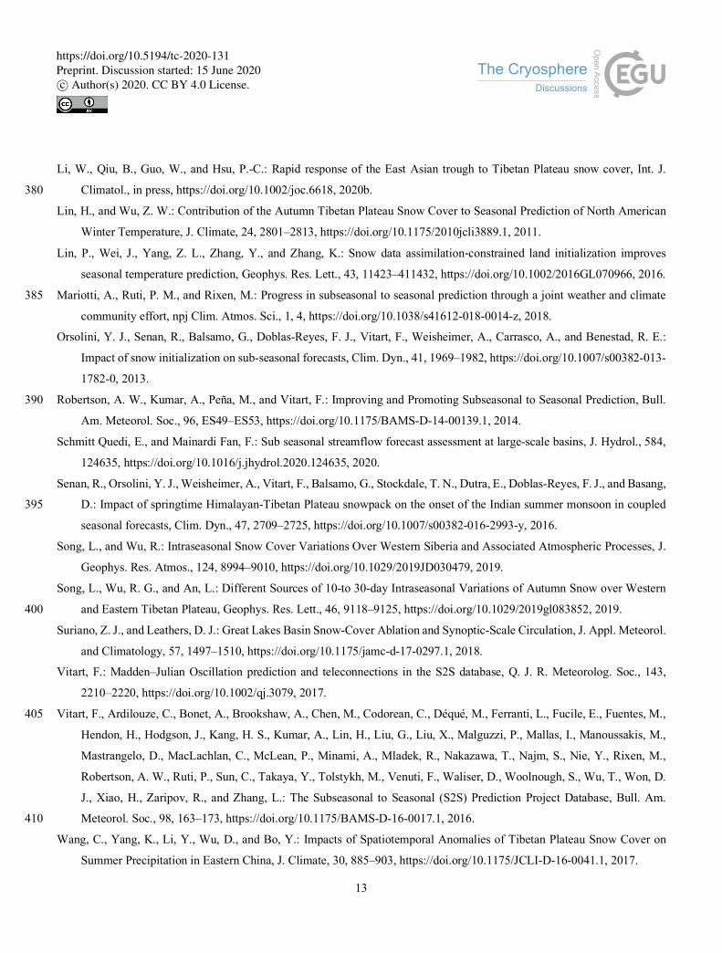
The Tibetan Plateau area of focus in this study is the region within 26–41°N and 70–105°E at an altitude of greater than

3000 m (Fig. 1). Although the Tibetan Plateau is located over middle latitudes, the area is cold due to high altitude, especially 90

in boreal winter. This study mainly focuses on TPSC during wintertime. Here, each winter contains 17 weeks, covering from

the 45th week (November 5–11) in one year to the 9th week (February 26–March 4) in the following year. This study spans

11 winters (from 1999/2000 to 2009/2010).


4

3 Tibetan Plateau snow cover in the S2S forecast models

3.1 Increasing Tibetan Plateau snow cover with forecast lead time 95

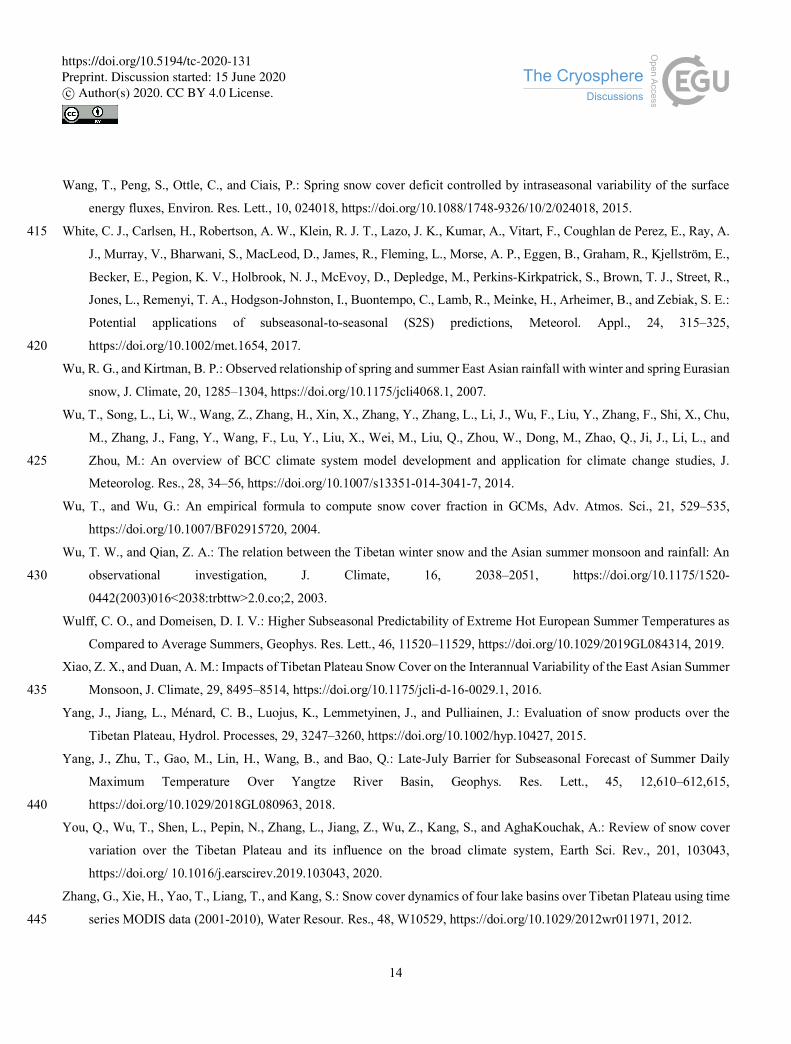
Before we present the systematic bias of TPSC in the S2S models, the overall forecast skills of TPSC is evaluated. Here, we

focus on the variation in snow-covered area over the entire Tibetan Plateau, which can be measured by a TPSC index. The

TPSC index represents the percentage of grid points covered by snow in the analysis or models over the entire Tibetan Plateau.

The unit of the TPSC index is %. The prediction skill of the TPSC index has been investigated through the temporal correlation

coefficient (TCC) between the TPSC index in the predictions and that in the observations during wintertime (Fig. 2). A skilful 100

prediction is generally defined as a TCC greater than 0.5. All three models show good prediction skills at lead times of 1–2

weeks with a TCC greater than 0.5. At lead times of 1–2 weeks, the TCC for the ECMWF model is largest among the three

models. The NCEP model has the lowest TCC among the three models at a lead time of 1 week. However, the TCC for NCEP

falls the most slowly at lead times of 2 weeks or more. The NCEP model has a larger TCC than the CMA model at lead times

of 2 weeks or more. The TCC values decrease with the increase in the forecast lead time and decline below 0.5 at and after 105

lead times of 3 weeks for all three models. These results indicate that the S2S models can skilfully forecast TPSC variations

within a lead time of 2 weeks during wintertime but show limited skill at a lead time of 3 weeks or more.

The seasonal cycle of TPSC is generally the most dominant component that contributes to the total variabilities in TPSC

(Li et al., 2020a). The prediction ability of models for the seasonal cycle of TPSC directly affects the prediction ability for the

total variability in TPSC. Systematic bias of TPSC in models will also be exposed in their multi-year mean seasonal cycle. 110

Because multi-year mean seasonal cycles of TPSC in the S2S models are based on only twelve years of available reforecasts

in this study, a 90-day low-pass filter is performed on the raw multi-year mean seasonal cycle to eliminate the unnecessary

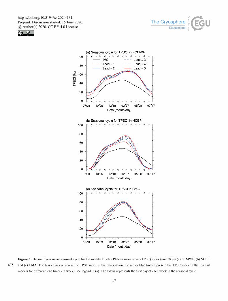
high-frequency signal. The seasonal cycle of TPSC indexes in IMS and three different models show some obvious differences

(Fig. 3). Models can generally reproduce the seasonal cycle of the TPSC index but with some non-negligible biases. Compared

with the IMS analysis, all models tend to overestimate the TPSC index during winter. The TPSC index in the ECMWF is 115

higher than the observed TPSC index by approximately 10–30% all year round (Fig. 3a). NCEP has a larger TPSC index than

that in the observation by approximately 10–30% during wintertime but tends to underestimate the TPSC index by

approximately 10% during summertime (Fig. 3b). CMA overestimates the TPSC index all year round (Fig. 3c), especially

during winter and spring (up to 30%). Overall, overestimation of the TPSC area is common in models compared with

observations, especially during winter. 120

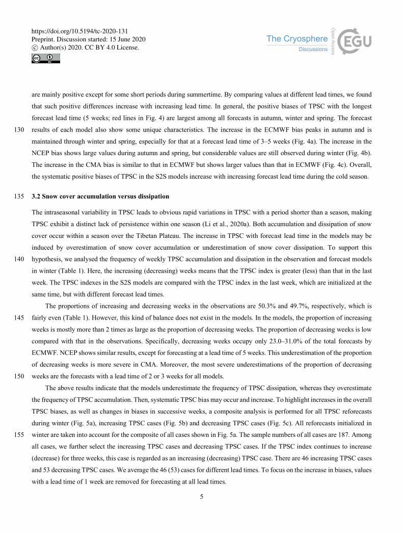
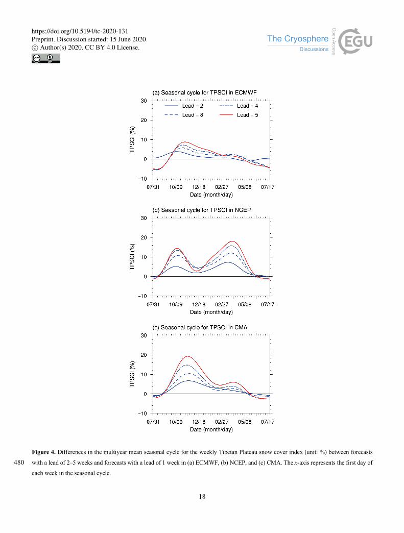
Another remarkable issue regarding the forecast of TPSC is the increasing TPSC with forecast lead time, which further

increases the overestimation of TPSC in models at longer forecast lead times. These increasing biases can be detected from

the multiyear mean seasonal cycle (Fig. 3). To highlight such increasing biases, we further present differences in the multiyear

mean seasonal cycle for the TPSC index between forecasts for leads of 2–5 weeks and forecasts for leads of 1 week in three

modes (Fig. 4). Such differences are obtained by subtracting the seasonal cycle at a lead time of 1 week from that at forecast 125

lead times of 2–5 weeks. The differences in the three models show some common features. The differences in all three models


5

are mainly positive except for some short periods during summertime. By comparing values at different lead times, we found

that such positive differences increase with increasing lead time. In general, the positive biases of TPSC with the longest

forecast lead time (5 weeks; red lines in Fig. 4) are largest among all forecasts in autumn, winter and spring. The forecast

results of each model also show some unique characteristics. The increase in the ECMWF bias peaks in autumn and is 130

maintained through winter and spring, especially for that at a forecast lead time of 3–5 weeks (Fig. 4a). The increase in the

NCEP bias shows large values during autumn and spring, but considerable values are still observed during winter (Fig. 4b).

The increase in the CMA bias is similar to that in ECMWF but shows larger values than that in ECMWF (Fig. 4c). Overall,

the systematic positive biases of TPSC in the S2S models increase with increasing forecast lead time during the cold season.

3.2 Snow cover accumulation versus dissipation 135

The intraseasonal variability in TPSC leads to obvious rapid variations in TPSC with a period shorter than a season, making

TPSC exhibit a distinct lack of persistence within one season (Li et al., 2020a). Both accumulation and dissipation of snow

cover occur within a season over the Tibetan Plateau. The increase in TPSC with forecast lead time in the models may be

induced by overestimation of snow cover accumulation or underestimation of snow cover dissipation. To support this

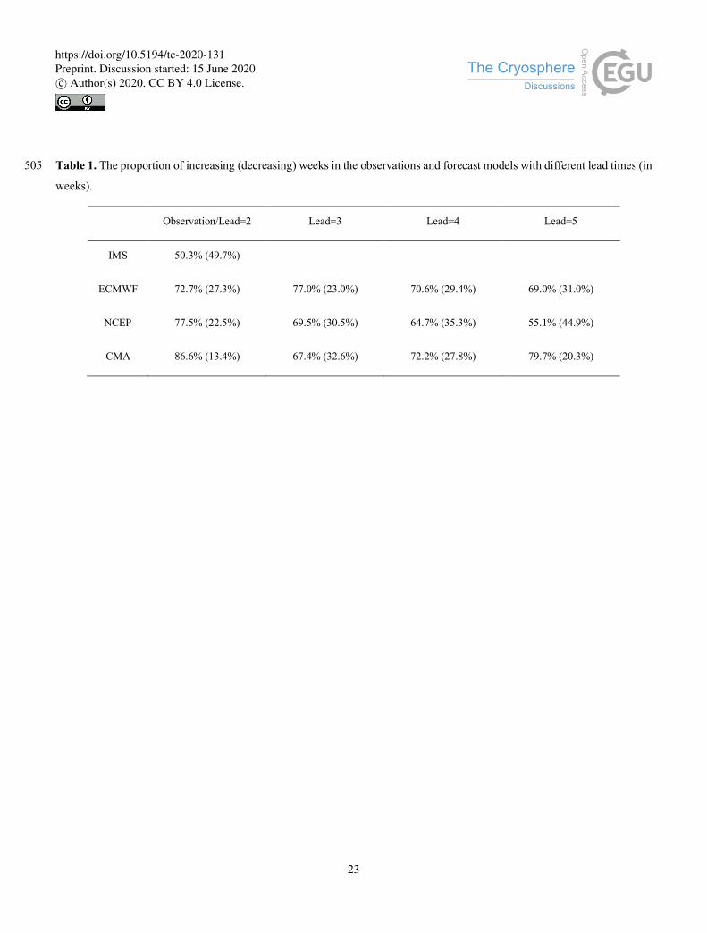
hypothesis, we analysed the frequency of weekly TPSC accumulation and dissipation in the observation and forecast models 140

in winter (Table 1). Here, the increasing (decreasing) weeks means that the TPSC index is greater (less) than that in the last

week. The TPSC indexes in the S2S models are compared with the TPSC index in the last week, which are initialized at the

same time, but with different forecast lead times.

The proportions of increasing and decreasing weeks in the observations are 50.3% and 49.7%, respectively, which is

fairly even (Table 1). However, this kind of balance does not exist in the models. In the models, the proportion of increasing 145

weeks is mostly more than 2 times as large as the proportion of decreasing weeks. The proportion of decreasing weeks is low

compared with that in the observations. Specifically, decreasing weeks occupy only 23.0–31.0% of the total forecasts by

ECMWF. NCEP shows similar results, except for forecasting at a lead time of 5 weeks. This underestimation of the proportion

of decreasing weeks is more severe in CMA. Moreover, the most severe underestimations of the proportion of decreasing

weeks are the forecasts with a lead time of 2 or 3 weeks for all models. 150

The above results indicate that the models underestimate the frequency of TPSC dissipation, whereas they overestimate

the frequency of TPSC accumulation. Then, systematic TPSC bias may occur and increase. To highlight increases in the overall

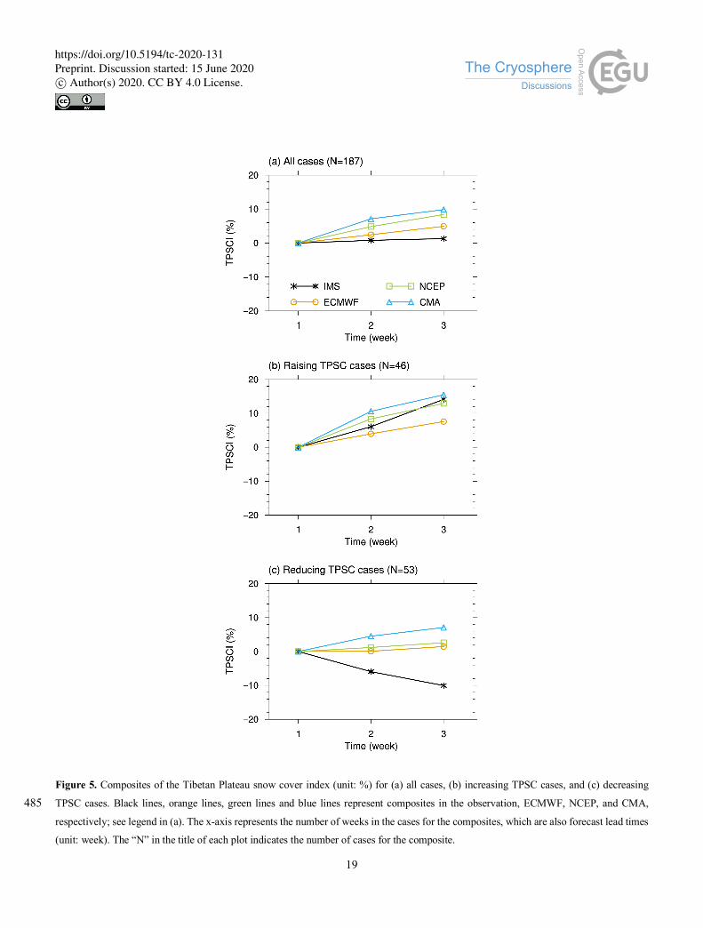
TPSC biases, as well as changes in biases in successive weeks, a composite analysis is performed for all TPSC reforecasts

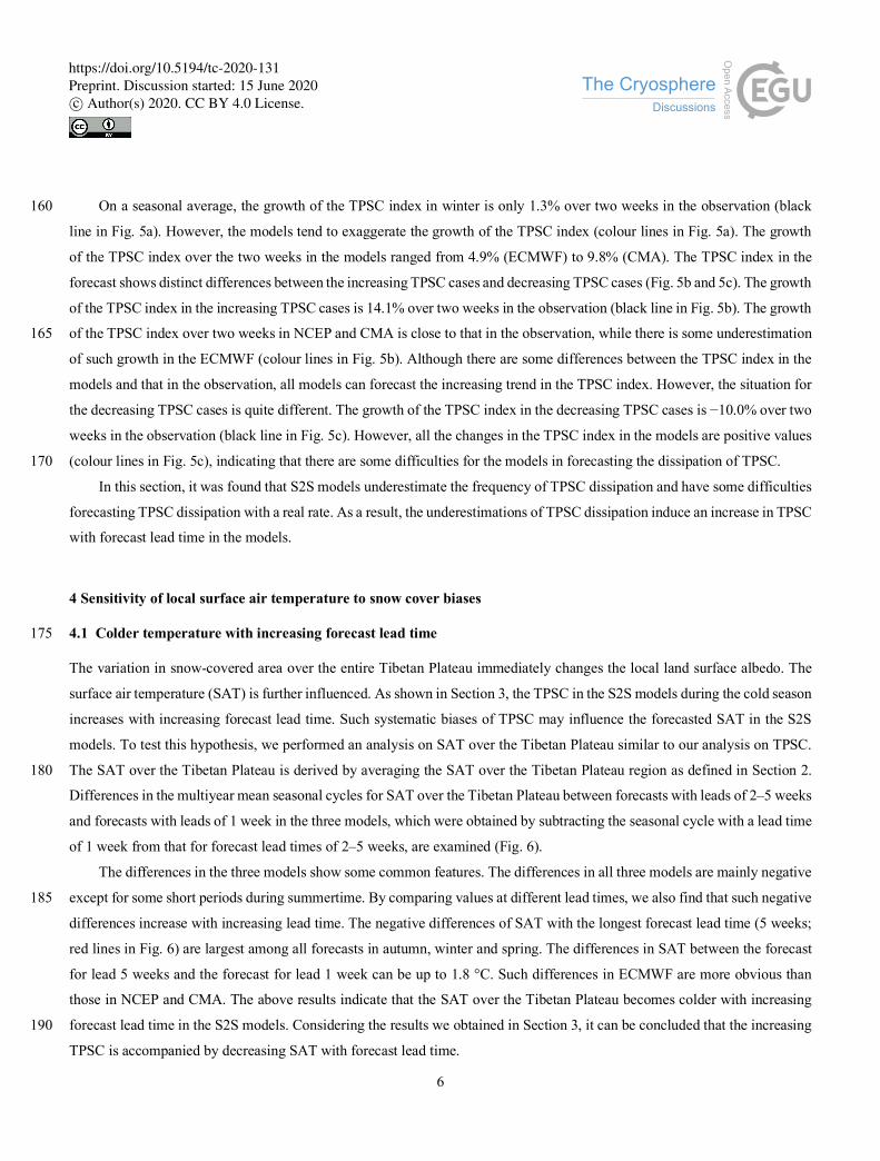
during winter (Fig. 5a), increasing TPSC cases (Fig. 5b) and decreasing TPSC cases (Fig. 5c). All reforecasts initialized in

winter are taken into account for the composite of all cases shown in Fig. 5a. The sample numbers of all cases are 187. Among 155

all cases, we further select the increasing TPSC cases and decreasing TPSC cases. If the TPSC index continues to increase

(decrease) for three weeks, this case is regarded as an increasing (decreasing) TPSC case. There are 46 increasing TPSC cases

and 53 decreasing TPSC cases. We average the 46 (53) cases for different lead times. To focus on the increase in biases, values

with a lead time of 1 week are removed for forecasting at all lead times.


6

On a seasonal average, the growth of the TPSC index in winter is only 1.3% over two weeks in the observation (black 160

line in Fig. 5a). However, the models tend to exaggerate the growth of the TPSC index (colour lines in Fig. 5a). The growth

of the TPSC index over the two weeks in the models ranged from 4.9% (ECMWF) to 9.8% (CMA). The TPSC index in the

forecast shows distinct differences between the increasing TPSC cases and decreasing TPSC cases (Fig. 5b and 5c). The growth

of the TPSC index in the increasing TPSC cases is 14.1% over two weeks in the observation (black line in Fig. 5b). The growth

of the TPSC index over two weeks in NCEP and CMA is close to that in the observation, while there is some underestimation 165

of such growth in the ECMWF (colour lines in Fig. 5b). Although there are some differences between the TPSC index in the

models and that in the observation, all models can forecast the increasing trend in the TPSC index. However, the situation for

the decreasing TPSC cases is quite different. The growth of the TPSC index in the decreasing TPSC cases is −10.0% over two

weeks in the observation (black line in Fig. 5c). However, all the changes in the TPSC index in the models are positive values

(colour lines in Fig. 5c), indicating that there are some difficulties for the models in forecasting the dissipation of TPSC. 170

In this section, it was found that S2S models underestimate the frequency of TPSC dissipation and have some difficulties

forecasting TPSC dissipation with a real rate. As a result, the underestimations of TPSC dissipation induce an increase in TPSC

with forecast lead time in the models.

4 Sensitivity of local surface air temperature to snow cover biases

4.1 Colder temperature with increasing forecast lead time 175

The variation in snow-covered area over the entire Tibetan Plateau immediately changes the local land surface albedo. The

surface air temperature (SAT) is further influenced. As shown in Section 3, the TPSC in the S2S models during the cold season

increases with increasing forecast lead time. Such systematic biases of TPSC may influence the forecasted SAT in the S2S

models. To test this hypothesis, we performed an analysis on SAT over the Tibetan Plateau similar to our analysis on TPSC.

The SAT over the Tibetan Plateau is derived by averaging the SAT over the Tibetan Plateau region as defined in Section 2. 180

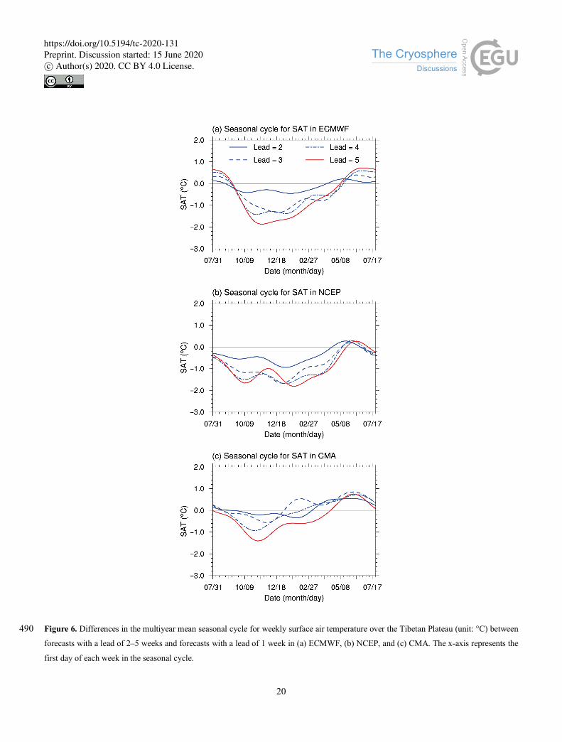
Differences in the multiyear mean seasonal cycles for SAT over the Tibetan Plateau between forecasts with leads of 2–5 weeks

and forecasts with leads of 1 week in the three models, which were obtained by subtracting the seasonal cycle with a lead time

of 1 week from that for forecast lead times of 2–5 weeks, are examined (Fig. 6).

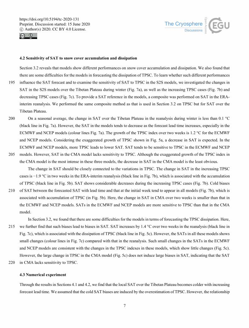
The differences in the three models show some common features. The differences in all three models are mainly negative

except for some short periods during summertime. By comparing values at different lead times, we also find that such negative 185

differences increase with increasing lead time. The negative differences of SAT with the longest forecast lead time (5 weeks;

red lines in Fig. 6) are largest among all forecasts in autumn, winter and spring. The differences in SAT between the forecast

for lead 5 weeks and the forecast for lead 1 week can be up to 1.8 °C. Such differences in ECMWF are more obvious than

those in NCEP and CMA. The above results indicate that the SAT over the Tibetan Plateau becomes colder with increasing

forecast lead time in the S2S models. Considering the results we obtained in Section 3, it can be concluded that the increasing 190

TPSC is accompanied by decreasing SAT with forecast lead time.


7

4.2 Sensitivity of SAT to snow cover accumulation and dissipation

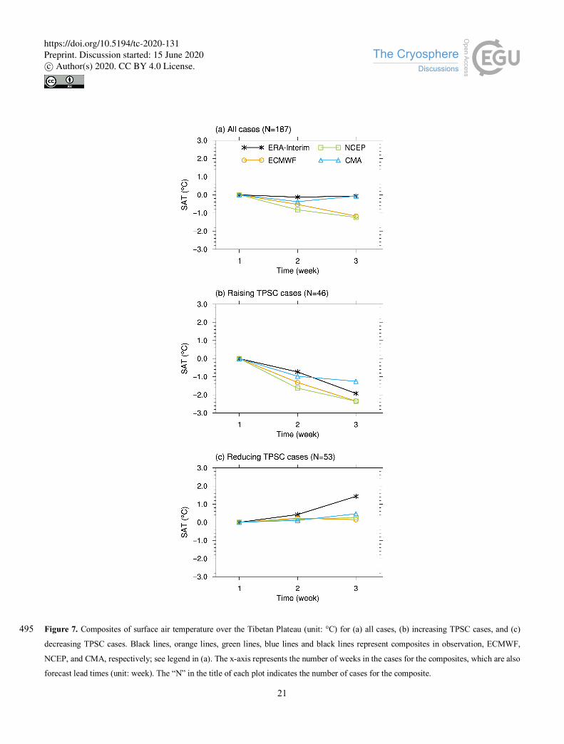
Section 3.2 reveals that models show different performances on snow cover accumulation and dissipation. We also found that

there are some difficulties for the models in forecasting the dissipation of TPSC. To learn whether such different performances

influence the SAT forecast and to examine the sensitivity of SAT to TPSC in the S2S models, we investigated the changes in 195

SAT in the S2S models over the Tibetan Plateau during winter (Fig. 7a), as well as the increasing TPSC cases (Fig. 7b) and

decreasing TPSC cases (Fig. 7c). To provide a SAT reference in the models, a composite was performed on SAT in the ERA-

interim reanalysis. We performed the same composite method as that is used in Section 3.2 on TPSC but for SAT over the

Tibetan Plateau.

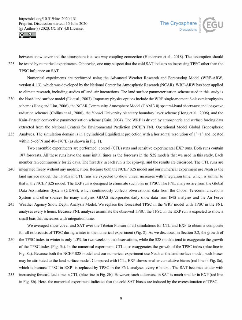
On a seasonal average, the change in SAT over the Tibetan Plateau in the reanalysis during winter is less than 0.1 °C 200

(black line in Fig. 7a). However, the SAT in the models tends to decrease as the forecast lead time increases, especially in the

ECMWF and NCEP models (colour lines Fig. 7a). The growth of the TPSC index over two weeks is 1.2 °C for the ECMWF

and NCEP models. Considering the exaggerated growth of TPSC shown in Fig. 5a, a decrease in SAT is expected. In the

ECMWF and NCEP models, more TPSC leads to lower SAT. SAT tends to be sensitive to TPSC in the ECMWF and NCEP

models. However, SAT in the CMA model lacks sensitivity to TPSC. Although the exaggerated growth of the TPSC index in 205

the CMA model is the most intense in these three models, the decrease in SAT in the CMA model is the least obvious.

The change in SAT should be closely connected to the variations in TPSC. The change in SAT in the increasing TPSC

cases is −1.9 °C in two weeks in the ERA-interim reanalysis (black line in Fig. 7b), which is associated with the accumulation

of TPSC (black line in Fig. 5b). SAT shows considerable decreases during the increasing TPSC cases (Fig. 7b). Cold biases

of SAT between the forecasted SAT with lead time and that at the initial week tend to appear in all models (Fig. 7b), which is 210

associated with accumulation of TPSC (in Fig. 5b). Here, the change in SAT in CMA over two weeks is smaller than that in

the ECMWF and NCEP models. SATs in the ECMWF and NCEP models are more sensitive to TPSC than that in the CMA

model.

In Section 3.2, we found that there are some difficulties for the models in terms of forecasting the TPSC dissipation. Here,

we further find that such biases lead to biases in SAT. SAT increases by 1.4 °C over two weeks in the reanalysis (black line in 215

Fig. 7c), which is associated with the dissipation of TPSC (black line in Fig. 5c). However, the SATs in all these models shows

small changes (colour lines in Fig. 7c) compared with that in the reanalysis. Such small changes in the SATs in the ECMWF

and NCEP models are consistent with the changes in the TPSC indexes in these models, which show little changes (Fig. 5c).

However, the large change in TPSC in the CMA model (Fig. 5c) does not induce large biases in SAT, indicating that the SAT

in CMA lacks sensitivity to TPSC. 220

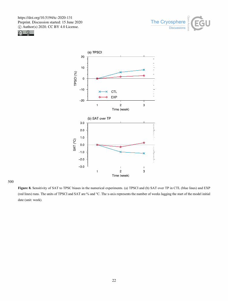
4.3 Numerical experiment

Through the results in Sections 4.1 and 4.2, we find that the local SAT over the Tibetan Plateau becomes colder with increasing

forecast lead time. We assumed that the cold SAT biases are induced by the overestimation of TPSC. However, the relationship


8

between snow cover and the atmosphere is a two-way coupling connection (Henderson et al., 2018). The assumption should

be tested by numerical experiments. Otherwise, one may suspect that the cold SAT induces an increasing TPSC other than the 225

TPSC influence on SAT.

Numerical experiments are performed using the Advanced Weather Research and Forecasting Model (WRF-ARW,

version 4.1.3), which was developed by the National Center for Atmospheric Research (NCAR). WRF-ARW has been applied

to climate research, including studies of land–air interactions. The land surface parameterization scheme used in this study is

the Noah land surface model (Ek et al., 2003). Important physics options include the WRF single-moment 6-class microphysics 230

scheme (Hong and Lim, 2006), the NCAR Community Atmosphere Model (CAM 3.0) spectral-band shortwave and longwave

radiation schemes (Collins et al., 2006), the Yonsei University planetary boundary layer scheme (Hong et al., 2006), and the

Kain–Fritsch convective parameterization scheme (Kain, 2004). The WRF is driven by atmospheric and surface forcing data

extracted from the National Centers for Environmental Prediction (NCEP) FNL Operational Model Global Tropospheric

Analyses. The simulation domain is in a cylindrical Equidistant projection with a horizontal resolution of 1°×1° and located 235

within 5–65°N and 40–170°E (as shown in Fig. 1).

Two ensemble experiments are performed: control (CTL) runs and sensitive experimental EXP runs. Both runs contain

187 forecasts. All these runs have the same initial times as the forecasts in the S2S models that we used in this study. Each

member ran continuously for 22 days. The first day in each run is for spin-up, and the results are discarded. The CTL runs are

integrated freely without any modification. Because both the NCEP S2S model and our numerical experiment use Noah as the 240

land surface model, the TPSCs in CTL runs are expected to show unreal increases with integration time, which is similar to

that in the NCEP S2S model. The EXP run is designed to eliminate such bias in TPSC. The FNL analyses are from the Global

Data Assimilation System (GDAS), which continuously collects observational data from the Global Telecommunications

System and other sources for many analyses. GDAS incorporates daily snow data from IMS analyses and the Air Force

Weather Agency Snow Depth Analysis Model. We replace the forecasted TPSC in the WRF model with TPSC in the FNL 245

analyses every 6 hours. Because FNL analyses assimilate the observed TPSC, the TPSC in the EXP run is expected to show a

small bias that increases with integration time.

We averaged snow cover and SAT over the Tibetan Plateau in all simulations for CTL and EXP to obtain a composite

for all reforecasts of TPSC during winter in the numerical experiment (Fig. 8). As we discussed in Section 3.2, the growth of

the TPSC index in winter is only 1.3% for two weeks in the observations, while the S2S models tend to exaggerate the growth 250

of the TPSC index (Fig. 5a). In the numerical experiment, CTL also exaggerates the growth of the TPSC index (blue line in

Fig. 8a). Because both the NCEP S2S model and our numerical experiment use Noah as the land surface model, such biases

may be attributed to the land surface model. Compared with CTL, EXP shows smaller cumulative biases (red line in Fig. 8a),

which is because TPSC in EXP is replaced by TPSC in the FNL analyses every 6 hours . The SAT becomes colder with

increasing forecast lead time in CTL (blue line in Fig. 8b). However, such a decrease in SAT is much smaller in EXP (red line 255

in Fig. 8b). Here. the numerical experiment indicates that the cold SAT biases are induced by the overestimation of TPSC.


9

5 Conclusion

Accurate subseasonal-to-seasonal (S2S) atmospheric forecasts and hydrological forecasts have considerable socioeconomic

value. This study evaluates the Tibetan Plateau snow cover (TPSC) prediction capabilities of three S2S forecast models

(ECMWF, NCEP and CMA). These three S2S models can skilfully forecast TPSC variations within a lead time of 2 weeks 260

during wintertime with temporal correlation coefficients greater than 0.5. ECMWF better captures TPSC variations compared

with NCEP and CMA at a lead time of 1–2 weeks. All models show limited skill in forecasting TPSC at a lead time of 3 weeks

or more. Compared with the IMS snow cover analysis, all three models tend to overestimate the area of TPSC, especially

during winter. Another remarkable issue regarding the TPSC forecast is the increasing TPSC with forecast lead time, which

makes the systematic positive biases of TPSC in models further increase at longer forecast lead times. Generally, the positive 265

biases of TPSC with the longest forecast lead time are largest among all forecasts with different lead times for most of the year.

S2S models underestimate the frequency of TPSC dissipation, whereas they overestimate the frequency of TPSC

accumulation. The accumulation and dissipation of wintertime TPSC occurs evenly in the observations. However, this kind of

balance does not exist in the S2S models. In the models, the proportion of TPSC accumulation is mostly more than 2 times as

large as the dissipation proportion. The most severe underestimations of the dissipation proportions are the forecasts at a lead 270

time of 2 or 3 weeks for all models. The models also have some difficulties forecasting the TPSC dissipation at a real rate. The

growth of TPSC in the decreasing TPSC cases is −10.0% over two weeks in the observations, but all the changes in TPSC in

the models are increasing. As a result, the underestimation of TPSC dissipation induces an increase in TPSC with forecast lead

time in the models.

The increasing TPSC is accompanied by decreasing surface air temperature (SAT) with forecast lead time. The SAT over 275

the Tibetan Plateau becomes colder with increasing forecast lead time in the S2S models. The negative differences in SATs

with the longest forecast lead times are largest among all forecasts in autumn, winter and spring. The differences in SATs

between the forecast for a lead of 5 weeks and the forecast for a lead of 1 week can be up to 1.8 °C. SATs tends to be sensitive

to the TPSCs in both ECMWF and NCEP. However, SAT in CMA lacks sensitivity to TPSC. Numerical experiments were

performed to test whether the cold SAT biases are induced by the TPSC overestimation. The control run exaggerates the 280

growth of TPSC, which is similar to that in S2S models. The SAT in the control run becomes colder with integration time.

When the increasing TPSC with forecast lead time in the models along with the integration of the model is removed in the

sensitivity run, the overestimated snow cover in the numerical model is flattened. Meanwhile, the decreasing SAT with

integration time also disappears. This finding indicates that cold SAT biases are induced by the TPSC overestimation.

Land–atmosphere coupling is one of the key physical processes for S2S prediction but is not well simulated and may 285

reduce S2S prediction skill (Robertson et al., 2014; Dirmeyer et al., 2019). Studies have shown that better snow cover

initialization improves subseasonal and seasonal forecasts/simulations (Jeong et al., 2013; Orsolini et al., 2013; Senan et al.,

2016; Lin et al., 2016; Kolstad, 2017). This study indicates that in addition to snow cover initialization, a better model skill for


10

snow cover prediction may also improves S2S prediction skill. More work is necessary and valuable to improve the prediction

ability of models for snow cover. 290

Data and code availability

The data and model used in this study are free to the public. The S2S datasets and ERA-interim data are available at

https://apps.ecmwf.int/datasets/. The IMS snow cover data are available at https://nsidc.org/data/G02156. The NCEP FNL data

are available at https://rda.ucar.edu/datasets/ds083.2/. The WRF source codes can be obtained at

https://www2.mmm.ucar.edu/wrf/users/download/get_source.html. All figures were produced using NCAR Command 295

Language (NCL) version 6.6.2, an open source software free to the public, by UCAR/NCAR/CISL/TDD,

https://doi.org/10.5065/d6wd3xh5. The NCL scripts used in this study are available from the corresponding author upon

reasonable request.

Author contribution

W.L. led the overall scientific questions and designed the research. S.H. and W.L. analyzed the data and drafted the manuscript. 300

Competing interests

The authors declare no competing interests.

Acknowledgements

This research is supported by the National Key Research and Development Program of China (2018YFC1505804), Natural

Science Foundation of China (41905074), the Natural Science Foundation of Jiangsu Province (BK20190782). 305

References

Balsamo, G., Beljaars, A., Scipal, K., Viterbo, P., van den Hurk, B., Hirschi, M., and Betts, A. K.: A Revised Hydrology for

the ECMWF Model: Verification from Field Site to Terrestrial Water Storage and Impact in the Integrated Forecast

System, J. Hydrometeorol., 10, 623–643, https://doi.org/10.1175/2008JHM1068.1, 2009.

Bamzai, A. S., and Shukla, J.: Relation between Eurasian Snow Cover, Snow Depth, and the Indian Summer Monsoon: An 310

Observational Study, J. Climate, 12, 3117–3132, https://doi.org/10.1175/1520-0442(1999)012<3117:RBESCS>2.0.CO;2,

1999.


11

Barnett, T. P., Dümenil, L., Schlese, U., Roeckner, E., and Latif, M.: The effect of Eurasian snow cover on regional and global

climate variations, J. Atmos. Sci., 46, 661–686, https://doi.org/10.1175/1520-0469(1989)046<0661:TEOESC>2.0.CO;2,

1989. 315

Chen, X. N., Long, D., Hong, Y., Liang, S. L., and Hou, A. Z.: Observed radiative cooling over the Tibetan Plateau for the

past three decades driven by snow cover-induced surface albedo anomaly, J. Geophys. Res. Atmos., 122, 6170–6185,

https://doi.org/10.1002/2017jd026652, 2017.

Clark, M. P., and Serreze, M. C.: Effects of variations in east Asian snow cover on modulating atmospheric circulation over

the north pacific ocean, J. Climate, 13, 3700–3710, https://doi.org/10.1175/1520-0442(2000)013<3700:eoviea>2.0.co;2, 320

2000.

Collins, W. D., Bitz, C. M., Blackmon, M. L., Bonan, G. B., Bretherton, C. S., Carton, J. A., Chang, P., Doney, S. C., Hack,

J. J., Henderson, T. B., Kiehl, J. T., Large, W. G., McKenna, D. S., Santer, B. D., and Smith, R. D.: The Community

Climate System Model version 3 (CCSM3), J. Climate, 19, 2122–2143, https://doi.org/10.1175/jcli3761.1, 2006.

de Andrade, F. M., Coelho, C. A. S., and Cavalcanti, I. F. A.: Global precipitation hindcast quality assessment of the 325

Subseasonal to Seasonal (S2S) prediction project models, Clim. Dyn., 52, 5451–5475, https://doi.org/10.1007/s00382-

018-4457-z, 2019.

Dee, D. P., Uppala, S. M., Simmons, A. J., Berrisford, P., Poli, P., Kobayashi, S., Andrae, U., Balmaseda, M. A., Balsamo, G.,

Bauer, P., Bechtold, P., Beljaars, A. C. M., van de Berg, L., Bidlot, J., Bormann, N., Delsol, C., Dragani, R., Fuentes, M.,

Geer, A. J., Haimberger, L., Healy, S. B., Hersbach, H., Holm, E. V., Isaksen, L., Kallberg, P., Koehler, M., Matricardi, 330

M., McNally, A. P., Monge-Sanz, B. M., Morcrette, J. J., Park, B. K., Peubey, C., de Rosnay, P., Tavolato, C., Thepaut,

J. N., and Vitart, F.: The ERA-Interim reanalysis: configuration and performance of the data assimilation system, Q. J. R.

Meteorolog. Soc., 137, 553–597, https://doi.org/10.1002/qj.828, 2011.

Dirmeyer, P. A., Gentine, P., Ek, M. B., and Balsamo, G.: Chapter 8 - Land Surface Processes Relevant to Sub-seasonal to

Seasonal (S2S) Prediction, in: Sub-Seasonal to Seasonal Prediction, edited by: Robertson, A. W., and Vitart, F., Elsevier, 335

165–181, 2019.

Dutra, E., Balsamo, G., Viterbo, P., Miranda, P. M. A., Beljaars, A., Schär, C., and Elder, K.: An Improved Snow Scheme for

the ECMWF Land Surface Model: Description and Offline Validation, J. Hydrometeorol., 11, 899–916,

https://doi.org/10.1175/2010JHM1249.1, 2010.

Ek, M. B., Mitchell, K. E., Lin, Y., Rogers, E., Grunmann, P., Koren, V., Gayno, G., and Tarpley, J. D.: Implementation of 340

Noah land surface model advances in the National Centers for Environmental Prediction operational mesoscale Eta model,

J. Geophys. Res. Atmos., 108, 8851, https://doi.org/10.1029/2002JD003296, 2003.

Fayad, A., Gascoin, S., Faour, G., López-Moreno, J. I., Drapeau, L., Page, M. L., and Escadafal, R.: Snow hydrology in

Mediterranean mountain regions: A review, J. Hydrol., 551, 374–396, https://doi.org/10.1016/j.jhydrol.2017.05.063,

2017. 345


12

Helfrich, S. R., McNamara, D., Ramsay, B. H., Baldwin, T., and Kasheta, T.: Enhancements to, and forthcoming developments

in the Interactive Multisensor Snow and Ice Mapping System (IMS), Hydrol. Processes, 21, 1576–1586,

https://doi.org/10.1002/hyp.6720, 2007.

Henderson, G. R., Peings, Y., Furtado, J. C., and Kushner, P. J.: Snow–atmosphere coupling in the Northern Hemisphere, Nat.

Clim. Change, 8, 954–963, https://doi.org/10.1038/s41558-018-0295-6, 2018. 350

Hong, S.-Y., and Lim, J.-O. J.: The WRF Single-Moment 6-Class Microphysics Scheme (WSM6), Asia-Pac. J. Atmos. Sci.,

42, 129–151, 2006.

Hong, S.-Y., Noh, Y., and Dudhia, J.: A new vertical diffusion package with an explicit treatment of entrainment processes,

Mon. Weather Rev., 134, 2318–2341, https://doi.org/10.1175/mwr3199.1, 2006.

Immerzeel, W. W., Droogers, P., de Jong, S. M., and Bierkens, M. F. P.: Large-scale monitoring of snow cover and runoff 355

simulation in Himalayan river basins using remote sensing, Remote Sens. Environ., 113, 40–49,

https://doi.org/10.1016/j.rse.2008.08.010, 2009.

Jeelani, G., Feddema, J. J., van der Veen, C. J., and Stearns, L.: Role of snow and glacier melt in controlling river hydrology

in Liddar watershed (western Himalaya) under current and future climate, Water Resour. Res., 48, W12508,

https://doi.org/10.1029/2011WR011590, 2012. 360

Jeong, J. H., Linderholm, H. W., Woo, S. H., Folland, C., Kim, B. M., Kim, S. J., and Chen, D. L.: Impacts of Snow

Initialization on Subseasonal Forecasts of Surface Air Temperature for the Cold Season, J. Climate, 26, 1956–1972,

https://doi.org/10.1175/jcli-d-12-00159.1, 2013.

Kain, J. S.: The Kain-Fritsch convective parameterization: An update, J. Appl. Meteorol., 43, 170–181,

https://doi.org/10.1175/1520-0450(2004)043<0170:tkcpau>2.0.co;2, 2004. 365

Kolstad, E. W.: Causal Pathways for Temperature Predictability from Snow Depth, J. Climate, 30, 9651–9663,

https://doi.org/10.1175/JCLI-D-17-0280.1, 2017.

Koren, V., Schaake, J., Mitchell, K., Duan, Q. Y., Chen, F., and Baker, J. M.: A parameterization of snowpack and frozen

ground intended for NCEP weather and climate models, J. Geophys. Res. Atmos., 104, 19569–19585,

https://doi.org/10.1029/1999JD900232, 1999. 370

Li, W., Chen, J., Li, L., Chen, H., Liu, B., Xu, C.-Y., and Li, X.: Evaluation and Bias Correction of S2S Precipitation for

Hydrological Extremes, J. Hydrometeorol., 20, 1887–1906, https://doi.org/10.1175/JHM-D-19-0042.1, 2019.

Li, W., Guo, W., Hsu, P.-C., and Xue, Y.: Influence of the Madden–Julian oscillation on Tibetan Plateau snow cover at the

intraseasonal time-scale, Sci. Rep., 6, 30456, https://doi.org/10.1038/srep30456, 2016.

Li, W., Guo, W., Qiu, B., Xue, Y., Hsu, P.-C., and Wei, J.: Influence of Tibetan Plateau snow cover on East Asian atmospheric 375

circulation at medium-range time scales, Nat. Commun., 9, 4243, https://doi.org/10.1038/s41467-018-06762-5, 2018.

Li, W., Qiu, B., Guo, W., Zhu, Z., and Hsu, P.-C.: Intraseasonal variability of Tibetan Plateau snow cover, Int. J. Climatol., in

press, https://doi.org/10.1002/joc.6407, 2020a.


13

Li, W., Qiu, B., Guo, W., and Hsu, P.-C.: Rapid response of the East Asian trough to Tibetan Plateau snow cover, Int. J.

Climatol., in press, https://doi.org/10.1002/joc.6618, 2020b. 380

Lin, H., and Wu, Z. W.: Contribution of the Autumn Tibetan Plateau Snow Cover to Seasonal Prediction of North American

Winter Temperature, J. Climate, 24, 2801–2813, https://doi.org/10.1175/2010jcli3889.1, 2011.

Lin, P., Wei, J., Yang, Z. L., Zhang, Y., and Zhang, K.: Snow data assimilation-constrained land initialization improves

seasonal temperature prediction, Geophys. Res. Lett., 43, 11423–411432, https://doi.org/10.1002/2016GL070966, 2016.

Mariotti, A., Ruti, P. M., and Rixen, M.: Progress in subseasonal to seasonal prediction through a joint weather and climate 385

community effort, npj Clim. Atmos. Sci., 1, 4, https://doi.org/10.1038/s41612-018-0014-z, 2018.

Orsolini, Y. J., Senan, R., Balsamo, G., Doblas-Reyes, F. J., Vitart, F., Weisheimer, A., Carrasco, A., and Benestad, R. E.:

Impact of snow initialization on sub-seasonal forecasts, Clim. Dyn., 41, 1969–1982, https://doi.org/10.1007/s00382-013-

1782-0, 2013.

Robertson, A. W., Kumar, A., Peña, M., and Vitart, F.: Improving and Promoting Subseasonal to Seasonal Prediction, Bull. 390

Am. Meteorol. Soc., 96, ES49–ES53, https://doi.org/10.1175/BAMS-D-14-00139.1, 2014.

Schmitt Quedi, E., and Mainardi Fan, F.: Sub seasonal streamflow forecast assessment at large-scale basins, J. Hydrol., 584,

124635, https://doi.org/10.1016/j.jhydrol.2020.124635, 2020.

Senan, R., Orsolini, Y. J., Weisheimer, A., Vitart, F., Balsamo, G., Stockdale, T. N., Dutra, E., Doblas-Reyes, F. J., and Basang,

D.: Impact of springtime Himalayan-Tibetan Plateau snowpack on the onset of the Indian summer monsoon in coupled 395

seasonal forecasts, Clim. Dyn., 47, 2709–2725, https://doi.org/10.1007/s00382-016-2993-y, 2016.

Song, L., and Wu, R.: Intraseasonal Snow Cover Variations Over Western Siberia and Associated Atmospheric Processes, J.

Geophys. Res. Atmos., 124, 8994–9010, https://doi.org/10.1029/2019JD030479, 2019.

Song, L., Wu, R. G., and An, L.: Different Sources of 10-to 30-day Intraseasonal Variations of Autumn Snow over Western

and Eastern Tibetan Plateau, Geophys. Res. Lett., 46, 9118–9125, https://doi.org/10.1029/2019gl083852, 2019. 400

Suriano, Z. J., and Leathers, D. J.: Great Lakes Basin Snow-Cover Ablation and Synoptic-Scale Circulation, J. Appl. Meteorol.

and Climatology, 57, 1497–1510, https://doi.org/10.1175/jamc-d-17-0297.1, 2018.

Vitart, F.: Madden–Julian Oscillation prediction and teleconnections in the S2S database, Q. J. R. Meteorolog. Soc., 143,

2210–2220, https://doi.org/10.1002/qj.3079, 2017.

Vitart, F., Ardilouze, C., Bonet, A., Brookshaw, A., Chen, M., Codorean, C., Déqué, M., Ferranti, L., Fucile, E., Fuentes, M., 405

Hendon, H., Hodgson, J., Kang, H. S., Kumar, A., Lin, H., Liu, G., Liu, X., Malguzzi, P., Mallas, I., Manoussakis, M.,

Mastrangelo, D., MacLachlan, C., McLean, P., Minami, A., Mladek, R., Nakazawa, T., Najm, S., Nie, Y., Rixen, M.,

Robertson, A. W., Ruti, P., Sun, C., Takaya, Y., Tolstykh, M., Venuti, F., Waliser, D., Woolnough, S., Wu, T., Won, D.

J., Xiao, H., Zaripov, R., and Zhang, L.: The Subseasonal to Seasonal (S2S) Prediction Project Database, Bull. Am.

Meteorol. Soc., 98, 163–173, https://doi.org/10.1175/BAMS-D-16-0017.1, 2016. 410

Wang, C., Yang, K., Li, Y., Wu, D., and Bo, Y.: Impacts of Spatiotemporal Anomalies of Tibetan Plateau Snow Cover on

Summer Precipitation in Eastern China, J. Climate, 30, 885–903, https://doi.org/10.1175/JCLI-D-16-0041.1, 2017.


14

Wang, T., Peng, S., Ottle, C., and Ciais, P.: Spring snow cover deficit controlled by intraseasonal variability of the surface

energy fluxes, Environ. Res. Lett., 10, 024018, https://doi.org/10.1088/1748-9326/10/2/024018, 2015.

White, C. J., Carlsen, H., Robertson, A. W., Klein, R. J. T., Lazo, J. K., Kumar, A., Vitart, F., Coughlan de Perez, E., Ray, A. 415

J., Murray, V., Bharwani, S., MacLeod, D., James, R., Fleming, L., Morse, A. P., Eggen, B., Graham, R., Kjellström, E.,

Becker, E., Pegion, K. V., Holbrook, N. J., McEvoy, D., Depledge, M., Perkins-Kirkpatrick, S., Brown, T. J., Street, R.,

Jones, L., Remenyi, T. A., Hodgson-Johnston, I., Buontempo, C., Lamb, R., Meinke, H., Arheimer, B., and Zebiak, S. E.:

Potential applications of subseasonal-to-seasonal (S2S) predictions, Meteorol. Appl., 24, 315–325,

https://doi.org/10.1002/met.1654, 2017. 420

Wu, R. G., and Kirtman, B. P.: Observed relationship of spring and summer East Asian rainfall with winter and spring Eurasian

snow, J. Climate, 20, 1285–1304, https://doi.org/10.1175/jcli4068.1, 2007.

Wu, T., Song, L., Li, W., Wang, Z., Zhang, H., Xin, X., Zhang, Y., Zhang, L., Li, J., Wu, F., Liu, Y., Zhang, F., Shi, X., Chu,

M., Zhang, J., Fang, Y., Wang, F., Lu, Y., Liu, X., Wei, M., Liu, Q., Zhou, W., Dong, M., Zhao, Q., Ji, J., Li, L., and

Zhou, M.: An overview of BCC climate system model development and application for climate change studies, J. 425

Meteorolog. Res., 28, 34–56, https://doi.org/10.1007/s13351-014-3041-7, 2014.

Wu, T., and Wu, G.: An empirical formula to compute snow cover fraction in GCMs, Adv. Atmos. Sci., 21, 529–535,

https://doi.org/10.1007/BF02915720, 2004.

Wu, T. W., and Qian, Z. A.: The relation between the Tibetan winter snow and the Asian summer monsoon and rainfall: An

observational investigation, J. Climate, 16, 2038–2051, https://doi.org/10.1175/1520-430

0442(2003)016<2038:trbttw>2.0.co;2, 2003.

Wulff, C. O., and Domeisen, D. I. V.: Higher Subseasonal Predictability of Extreme Hot European Summer Temperatures as

Compared to Average Summers, Geophys. Res. Lett., 46, 11520–11529, https://doi.org/10.1029/2019GL084314, 2019.

Xiao, Z. X., and Duan, A. M.: Impacts of Tibetan Plateau Snow Cover on the Interannual Variability of the East Asian Summer

Monsoon, J. Climate, 29, 8495–8514, https://doi.org/10.1175/jcli-d-16-0029.1, 2016. 435

Yang, J., Jiang, L., Ménard, C. B., Luojus, K., Lemmetyinen, J., and Pulliainen, J.: Evaluation of snow products over the

Tibetan Plateau, Hydrol. Processes, 29, 3247–3260, https://doi.org/10.1002/hyp.10427, 2015.

Yang, J., Zhu, T., Gao, M., Lin, H., Wang, B., and Bao, Q.: Late-July Barrier for Subseasonal Forecast of Summer Daily

Maximum Temperature Over Yangtze River Basin, Geophys. Res. Lett., 45, 12,610–612,615,

https://doi.org/10.1029/2018GL080963, 2018. 440

You, Q., Wu, T., Shen, L., Pepin, N., Zhang, L., Jiang, Z., Wu, Z., Kang, S., and AghaKouchak, A.: Review of snow cover

variation over the Tibetan Plateau and its influence on the broad climate system, Earth Sci. Rev., 201, 103043,

https://doi.org/ 10.1016/j.earscirev.2019.103043, 2020.

Zhang, G., Xie, H., Yao, T., Liang, T., and Kang, S.: Snow cover dynamics of four lake basins over Tibetan Plateau using time

series MODIS data (2001-2010), Water Resour. Res., 48, W10529, https://doi.org/10.1029/2012wr011971, 2012. 445


15

Zhang, L. L., Su, F. G., Yang, D. Q., Hao, Z. C., and Tong, K.: Discharge regime and simulation for the upstream of major

rivers over Tibetan Plateau, J. Geophys. Res. Atmos., 118, 8500–8518, https://doi.org/10.1002/jgrd.50665, 2013.

Zhang, T. J.: Influence of the seasonal snow cover on the ground thermal regime: An overview, Rev. Geophys., 43, RG4002,

https://doi.org/10.1029/2004rg000157, 2005.

Zhang, Y., Zou, T., and Xue, Y.: An Arctic-Tibetan Connection on Subseasonal to Seasonal Time Scale, Geophys. Res. Lett., 450

46, 2790–2799, https://doi.org/10.1029/2018GL081476, 2019.


16

Figure 1. The location and topography of the Tibetan Plateau. Shading shows topography (unit: m). The black rectangle shows the region 455 within 26–41°N and 70–105°E. The red contour marks altitudes at 3000 m. The Tibetan Plateau area, which is the focus of this study is the

region within the black rectangle at an altitude of greater than 3000 m. This figure also shows the simulation domain for numerical

experiments in this study.

460

465 Figure 2. Prediction skill of the Tibetan Plateau snow cover (TPSC) index in the S2S models during wintertime. The temporal correlation

coefficients (TCCs; y-axis) between the observed TPSC index and the predicted TPSC index in the ECMWF (orange line), NCEP (green

line) and CMA (blue line) models during winter. The x-axis represents the forecast lead time (unit: week). A good prediction skill has a TCC

that is greater than 0.5 (marked by black line). 470


17

Figure 3. The multiyear mean seasonal cycle for the weekly Tibetan Plateau snow cover (TPSC) index (unit: %) in (a) ECMWF, (b) NCEP,

and (c) CMA. The black lines represent the TPSC index in the observation; the red or blue lines represent the TPSC index in the forecast 475 models for different lead times (in week); see legend in (a). The x-axis represents the first day of each week in the seasonal cycle.


18

Figure 4. Differences in the multiyear mean seasonal cycle for the weekly Tibetan Plateau snow cover index (unit: %) between forecasts

with a lead of 2–5 weeks and forecasts with a lead of 1 week in (a) ECMWF, (b) NCEP, and (c) CMA. The x-axis represents the first day of 480 each week in the seasonal cycle.


19

Figure 5. Composites of the Tibetan Plateau snow cover index (unit: %) for (a) all cases, (b) increasing TPSC cases, and (c) decreasing

TPSC cases. Black lines, orange lines, green lines and blue lines represent composites in the observation, ECMWF, NCEP, and CMA, 485 respectively; see legend in (a). The x-axis represents the number of weeks in the cases for the composites, which are also forecast lead times

(unit: week). The “N” in the title of each plot indicates the number of cases for the composite.


20

Figure 6. Differences in the multiyear mean seasonal cycle for weekly surface air temperature over the Tibetan Plateau (unit: °C) between 490 forecasts with a lead of 2–5 weeks and forecasts with a lead of 1 week in (a) ECMWF, (b) NCEP, and (c) CMA. The x-axis represents the

first day of each week in the seasonal cycle.


21

Figure 7. Composites of surface air temperature over the Tibetan Plateau (unit: °C) for (a) all cases, (b) increasing TPSC cases, and (c) 495 decreasing TPSC cases. Black lines, orange lines, green lines, blue lines and black lines represent composites in observation, ECMWF,

NCEP, and CMA, respectively; see legend in (a). The x-axis represents the number of weeks in the cases for the composites, which are also

forecast lead times (unit: week). The “N” in the title of each plot indicates the number of cases for the composite.


22

500 Figure 8. Sensitivity of SAT to TPSC biases in the numerical experiments. (a) TPSCI and (b) SAT over TP in CTL (blue lines) and EXP

(red lines) runs. The units of TPSCI and SAT are % and °C. The x-axis represents the number of weeks lagging the start of the model initial

date (unit: week).


23

Table 1. The proportion of increasing (decreasing) weeks in the observations and forecast models with different lead times (in 505

weeks).

Observation/Lead=2 Lead=3 Lead=4 Lead=5

IMS 50.3% (49.7%)

ECMWF 72.7% (27.3%) 77.0% (23.0%) 70.6% (29.4%) 69.0% (31.0%)

NCEP 77.5% (22.5%) 69.5% (30.5%) 64.7% (35.3%) 55.1% (44.9%)

CMA 86.6% (13.4%) 67.4% (32.6%) 72.2% (27.8%) 79.7% (20.3%)


Documents

Systematic bias of Tibetan Plateau snow cover in subseasonal