Table 3.1 lists the 33 NUTS-2 regions by country and the

AlpenCorSAlpen Corridor South

D 5

Modelling Regional Development in AlpenCorSScenario Results

Final Report

Dortmund, January 2005Revised: June 2005

Spiekermann & WegenerUrban and Regional ResearchLindemannstrasse 10 Tel.: +49 0231 1899 441D-44137 Dortmund Fax. +49 0231 1899 443

2

Table of Contents

1. Introduction ............................................................................................................................. 3

2. The SASI Model ..................................................................................................................... 52.1 Model Design .................................................................................................................. 52.2 Model Output .................................................................................................................. 72.3 Model Developments for AlpenCorS .............................................................................. 72.4 Model Calibration ............................................................................................................ 8

3. The Study Area ........................................................................................................................ 10

4. Scenarios ................................................................................................................................ 164.1 The Reference Scenario (Scenario 000) ........................................................................ 164.2 Infrastructure Scenarios ................................................................................................. 16

4.2.1 The Brenner Tunnel (Scenario AS1) .................................................................... 164.2.2 Southern Rail Bypass (Scenario AS2) ................................................................. 204.2.3 Motorways Valdastico and Pedemontana (Scenario AS3) .................................. 204.2.4 Valsugana Road and Rail Corridor (Scenario AS4) ............................................. 214.2.5 Combination Scenario AS1+AS2+AS3+AS4 (Scenario AS5) ............................. 214.2.6 Other European Infrastructure Improvements (Scenario AS6) ............................ 21

5. Scenario Results ..................................................................................................................... 235.1 The Reference Scenario (Scenario 000) ........................................................................ 235.2 Infrastructure Scenarios ................................................................................................. 33

5.2.1 Effects of the Brenner tunnel (Scenario AS1) ...................................................... 335.2.2 Effects of other Transport Projects (Scenarios AS2 to AS6) ............................... 38

6. Scenario Comparison .............................................................................................................. 46

7. Territorial Cohesion ................................................................................................................. 57

8. Conclusions ............................................................................................................................. 63

References ................................................................................................................................... 65

Appendix: System of Regions in AlpenCorS ................................................................................ 68

3

1 Introduction

AlpenCorS is a multi-sectoral and inter-regional bottom-up development project of economy andtransport matters focused on the central segment of the Paneuropean Corridor V betweenFrance, Italy and Slovenia-Austria south of the Alps. The AlpenCorS project is being conductedwithin the Interreg III B Programme "Alpine Space" (2000-2006).

AlpencorS aims at contributing to the development of a Corridor policy concept as a commonstrategy of economic and space development for this part of the European territory. The researchpresented in this report contributes to Work Package 10 of AlpenCorS. The objective of WorkPackage 10 is to contribute to the AlpenCorS strategy by assessing the potential of the intersec-tion of Corridor V with the major trans-Alpine north-south corridor linking the AlpenCorS regionswith the European regions north of the Alps, Corridor I, the Brenner corridor. The projections ofthe regional economic impacts of various transport policy options for the Brenner corridor pre-sented in this report contribute to a broader Territorial Impact Assessment of these policy optionsproduced at the Dipartimento di Ingegneria Gestionale of the Politecnico di Milano aiming at un-covering the general economic and transport evolution within Corridor I and providing basic in-formation for future corridor policy.

Scenarios of future economic development in the regions within and outside the AlpenCorS studyarea are a prerequisite for making forecasts of the development of travel and goods transport inthe Corridor. However, regional economic development is itself a function of the efficiency of thetransport system in the Corridor and of how the Corridor is linked with the rest of the Europeanterritory. Forecasting regional economic development in the Corridor therefore requires a fore-casting model able to capture the interaction between spatial development and transport.

The SASI model presented in this report is a model of this kind. The SASI model is used to fore-cast economic development in the regions within and outside the Corridor subject to (a) assump-tions about economic development in Europe at large, (b) assumptions about the process ofEuropean integration in particular with respect to the new EU member states and future potentialaccession countries and (c) assumptions about the implementation of European and nationalpolicies in the fields of economic policy, migration policy and transport policy, and to analyse theeffects of these scenarios on interregional cohesion, i.e. socio-economic convergence betweenthe regions.

The First Interim Report (June 2004) presented the structure of the SASI model and of its data-base as it was developed and applied in previous EU projects, in particular the projects IASON(Integrated Appraisal of Spatial Economic and Network Effects of Transport Investments andPolicies) of the 5th Research Framework of the European Union and ESPON 2.1.1 (TerritorialImpacts EU Transport and TEN Policies) of the European Spatial Planning Observation Network(ESPON). In addition, the study area analysed in AlpenCorS and the extensions of the modeldatabase performed to prepare the model for the tasks in AlpenCorS were presented in tablesand maps.

The Second Interim Report (December 2004) presented first results of the application of the SASImodel to the AlpenCorS study area. In that report only two transport policy scenarios could bepresented. This Final Report presents the results of a larger set of transport policy scenarios, in-cluding those incorporating the implementation of the Valdastico and Pedemontana Venetamotorways and the development of the Valsugana road and rail corridor. This final set of scenar-ios was made compatible with the scenarios examined in the Territorial Impact Assessment con-ducted by at the Dipartimento di Ingegneria Gestionale of the Politecnico di Milano.

4

This report starts with a brief recapitulation of the SASI model, its further development for Alpen-CorS and the character of its results. It then presents the reference scenario, which serves as thebenchmark for the comparison of the transport infrastructure scenarios to be studied. Typical out-put indicators of the reference scenario are presented in diagrams and maps with special focuson the AlpenCorS regions and in particular the Autonomous Provinces of Trento and Bolzano.Then the transport infrastructure scenarios studied are explained and their results presented andcompared. The report closes with a discussion of the relevance and reliability of the results andtheir implications for a coherent Corridor strategy.

The work reported is the outcome of a co-operation with the Dipartimento di Ingegneria Gestion-ale of the Politecnico di Milano. The support by Roberto Camagni and Tomaso Pompili is grate-fully acknowledged. At the Provincia Autonoma di Trento, Claudio Tiso and Maurizio Castagniniprovided valuable information and helpful guidance. Maria Teresa Gabardi and her colleagues atthe Dipartimento Interateneo Territorio (DIT) at the Politecnico and Università di Torino kindlyprovided information on transport infrastructure projects in the AlpenCorS area for cross-checkingthe European network database used with the SASI model. Special thanks go to Carsten Schür-mann of RRG Spatial Planning and Geoinformation for integrating this information and specifyingthe transport infrastructure scenarios in that database.

Klaus SpiekermannMichael Wegener

5

2 The SASI Model

There exists a broad spectrum of theoretical approaches to explain the impacts of transport infra-structure investments on regional socio-economic development. Originating from different scien-tific disciplines and intellectual traditions, these approaches presently coexist, even though theyare partially in contradiction (cf. Linnecker, 1997):

- National growth approaches model multiplier effects of public investment in which public invest-ment, such as transport investment, has a positive influence on private investment.

- Regional growth approaches assume that regional economic growth is a function of regionalendowment factors including public capital such as transport infrastructure.

- Production function approaches model economic activity in a region as a function of productionfactors including infrastructure as a public input used by firms within the region.

- Accessibility approaches substitute more complex accessibility indicators for the simple infra-structure endowment in the regional production function.

- Regional input-output approaches model interregional and inter-industry linkages as a functionof transport cost and technical inter-industry input-output coefficients.

- Trade integration approaches model interregional trade flows as a function of interregionaltransport costs and regional product prices.

The SASI model belongs to the group of accessibility approaches in which regional productionfunctions are extended by accessibility indicators representing the locational advantage of re-gions provided by the transport system. In this chapter, the SASI model is briefly presented. Amore comprehensive description of the model is contained in AlpenCorS Deliverable D2.2 Model-ling Regional Development in AlpenCorS: Construction of the Economic Impact Model (Spieker-mann and Wegener, 2004).

2.1 Model Design

The SASI model (Wegener and Bökemann, 1998; Bröcker et al., 2002) is a recursive simulationmodel of socio-economic development of regions in Europe subject to exogenous assumptionsabout the economic and demographic development of the European Union as a whole and trans-port infrastructure investments and transport system improvements, in particular of the trans-European transport networks..

The main concept of the SASI model is to explain locational structures and locational change inEurope in combined time-series/cross-section regressions, with accessibility indicators being asubset of a range of explanatory variables. The focus of the regression approach is on long-termspatial distributional effects of transport policies. Factors of production including labour, capitaland knowledge are considered as mobile in the long run, and the model incorporates determi-nants of the redistribution of factor stocks and population. The model is therefore suitable tocheck whether long-run tendencies in spatial development coincide with the spatial developmentobjectives of the European Union. Its application is restricted, however, in other respects: Themodel generates mainly distributive and only to a limited extent generative effects of transportcost reductions, and it does not produce regional welfare assessments fitting into the frameworkof cost-benefit analysis.

6

The SASI model differs from other approaches to model the impacts of transport on regional de-velopment by modelling not only production (the demand side of regional labour markets) but alsopopulation (the supply side of regional labour markets), which makes it possible to model regionalunemployment. A second distinct feature is its dynamic network database based on a 'strategic'subset of highly detailed pan-European road, rail and air networks including major historical net-work changes as far back as 1981 and forecasting expected network changes according to themost recent EU documents on the future evolution of the trans-European transport networks.

The SASI model has six forecasting submodels: European Developments, Regional Accessibility,Regional GDP, Regional Employment, Regional Population and Regional Labour Force. A sev-enth submodel calculates Socio-Economic Indicators with respect to efficiency and equity. Figure2.1 visualises the interactions between these submodels.

Figure 2.1. The SASI model

The spatial dimension of the model is established by the subdivision of the 25 present countriesof the European Union plus Norway and Switzerland and the two candidate countries Bulgariaand Romania and for AlpenCorS also the five western Balkan countries Albania, Bosnia and Her-zegowina, Croatia, Makedonia and Yugoslavia into 1,330 regions and by connecting these byroad, rail and air networks. For each region the model forecasts the development of accessibilityand GDP per capita. In addition cohesion indicators expressing the impact of transport infra-structure investments and transport system improvements on the convergence (or divergence) ofsocio-economic development in the regions of the European Union are calculated.

7

The temporal dimension of the model is established by dividing time into periods of one year du-ration. By modelling relatively short time periods both short- and long-term lagged impacts can betaken into account. In each simulation year the seven submodels of the SASI model are proc-essed in a recursive way, i.e. sequentially one after another. This implies that within one simula-tion period no equilibrium between model variables is established; in other words, all endogenouseffects in the model are lagged by one or more years.

2.2 Model Output

The main output of the SASI model are accessibility and GDP per capita for each region for eachyear of the simulation. However, a great number of other regional indicators are generated duringthe simulation. These indicators can be examined during the simulation by observing time-seriesdiagrams, choropleth maps or 3D representations of variables of interest on the computer display.The user may interactively change the selection of variables to be displayed during processing.The same selection of variables can be analysed and post-processed after the simulation. If severalscenarios have been simulated, the user can compare the results using a special comparison soft-ware.

2.3 Model Developments for AlpenCorS

The SASI model was applied in the projects IASON (Integrated Appraisal of Spatial Economicand Network Effects of Transport Investments and Policies) of the 5th Research Framework ofthe European Union (Bröcker et al., 2004a) and ESPON 2.1.1 (Territorial Impacts EU Transportand TEN Policies) of the European Spatial Planning Observation Network ESPON (Bröcker et al.,2003, 2004b).

For its application in AlpenCorS three extensions of the model database were performed to makethe model better prepared for the tasks in AlpenCorS:

(1) The system of regions of the model was extended to include the western Balkan countriesAlbania, Bosnia and Herzegowina, Croatia, Makedonia and Yugoslavia. By this the numberof regions considered in the model was increased to 1,330.

(2) The network database of the model was represented in greater detail in the AlpenCorS studyarea in order to make the model more sensitive to local improvements.

(3) The model database was updated using recently made available regional data for GDP, em-ployment and population for the year 2001.

(4) The regional production functions of the model were re-calibrated using the 2001 data. Theresults of the new calibration are presented in the following section.

8

2.4 Model Calibration

The regional production functions of the SASI model were estimated by linear regression of thelogarithmically transformed Cobb-Douglas regional production functions for the 1,330 internal re-gions and the six industrial sectors used in AlpenCorS for the years 1981, 1986, 1991, 1996 and2001. The dependent variable is regional GDP per capita in 1,000 Euro of 1998.

Because of numerous gaps and inconsistencies in the data, extensive research was necessary tosubstitute missing or inconsistent data by estimation or by analogy with similar regions. In par-ticular for the accession countries in eastern Europe, which underwent the transition from plannedeconomies to market economies, information on regional GDP was inconsistent or completelymissing. It was therefore necessary to adjust regional sectoral GDP data for the years 1981 to1991 to conform to estimates of regional GDP totals by Eurostat. In a similar way the sectoralcomposition of regional economies was cross-checked by comparison with the sectoral composi-tion of gross value added in the Eurostat New Cronos database.

The independent variables of the regressions were a large set of regional indicators of potentialexplanatory value from which the following were selected:

sgdpn Share of GDP of sector n (%)gdpwn GDP per worker in sector n (1,000 Euro of 1998)acct Accessibility road/rail/air travelaccf Accessibility road/rail freightrlmp Regional labour market potential (accessibility to labour)pdens Population density (pop/ha)devld Developed land (%)rdinv R&D investment (% of GDP)eduhi Share of population with higher education (%)quali Quality of life indicator (0-100)

To take account of the slow process of economic structural change, independent variables sgdpnand gdpwn are lagged by five years; all other independent variables are lagged by one year, i.e.the most recent available value is taken. Because no data are available for years before 1981, nolags are applied for 1981.

Table 2.1 shows the regression coefficients for the selected variables for 2001. Given the largenumber of regions and the exclusion of region size by the choice of GDP per capita as dependentvariable, the results are very satisfactory.

In the simulations for the years 1981 to 2001, predicted GDP values were corrected by their re-siduals to match observed values. The regression parameters and residuals for 2001 were usedfor the simulations for the years 2002 to 2021.

9

Table 2.1. SASI model: calibration results (2001)

Regression coefficients

VariablesAgriculture Manufac-

turingConstruc-

tion

Trade,tourism,transport

Financialservices

Otherservices

sgdpngdpwnacctacctfrlmppdensdevldrdinveduhiqualiConstant

0.4840660.529735

0.396847

–0.156644

–2.608195

0.9923860.850462

0.1619510.050725

0.1014370.123613

–1.379831

1.1644690.935339

0.264272

0.035371

–1.734054

1.0867560.8743630.261673

0.057370–0.036171–0.145818

0.341000–1.510096

1.2230990.3173790.123609

0.0354580.032480

0.3078330.607406

1.667133

1.1427650.8740440.224719

0.049688

0.0861430.110765

–1.325561

r2 0.635 0.581 0.644 0.676 0.614 0.711

10

3 The Study Area

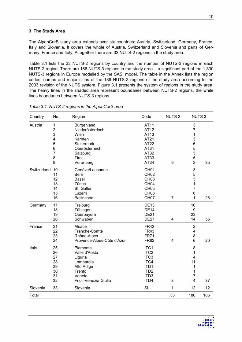
The AlpenCorS study area extends over six countries: Austria, Switzerland, Germany, France,Italy and Slovenia. It covers the whole of Austria, Switzerland and Slovenia and parts of Ger-many, France and Italy. Altogether there are 33 NUTS-2 regions in the study area.

Table 3.1 lists the 33 NUTS-2 regions by country and the number of NUTS-3 regions in eachNUTS-2 region. There are 186 NUTS-3 regions in the study area – a significant part of the 1,330NUTS-3 regions in Europe modelled by the SASI model. The table in the Annex lists the regioncodes, names and major cities of the 186 NUTS-3 regions of the study area according to the2003 revision of the NUTS system. Figure 3.1 presents the system of regions in the study area.The heavy lines in the shaded area represent boundaries between NUTS-2 regions, the whitelines boundaries between NUTS-3 regions.

Table 3.1. NUTS-2 regions in the AlpenCorS area

Country No. Region Code NUTS 2 NUTS 3

Austria 1 Burgenland AT11 32 Niederösterriech AT12 73 Wien AT13 14 Kärnten AT21 35 Steiermark AT22 66 Oberösterreich AT31 57 Salzburg AT32 38 Tirol AT33 59 Vorarlberg AT34 9 2 35

Switzerland 10 Genève/Lausanne CH01 311 Bern CH02 512 Basel CH03 313 Zürich CH04 114 St. Gallen CH05 715 Luzern CH06 616 Bellinzona CH07 7 1 26

Germany 17 Freiburg DE13 1018 Tübingen DE14 919 Oberbayern DE21 2320 Schwaben DE27 4 14 56

France 21 Alsace FR42 222 Franche-Comté FR43 423 Rhône-Alpes FR71 824 Provence-Alpes-Côte d'Azur FR82 4 6 20

Italy 25 Piemonte ITC1 826 Valle d'Aosta ITC2 127 Liguria ITC3 428 Lombardia ITC4 1129 Alto Adige ITD1 130 Trento ITD2 131 Veneto ITD3 732 Friuli-Venezia Giulia ITD4 8 4 37

Slovenia 33 Slovenia SI 1 12 12

Total 33 186 186

11

The transport networks used with the SASI model rely on the European transport network GISdatabase developed by the Institute of Spatial Planning of the University of Dortmund (IRPUD,2001). The strategic road and rail networks used in the model comprise the trans-Europeantransport networks (TEN-T) specified in Decision 1692/96/EC of the European Parliament and ofthe Council (European Communities, 1996; European Commission, 1998), further specified in theTEN Implementation Report and latest revisions of the TEN guidelines provided by the EuropeanCommission (2002a; 2002b) and the latest documents on the priority projects (High Level Group,2003; European Commission, 2003; 2004) and the transport networks of European importanceidentified in eastern Europe by the Transport Needs Assessment (TINA) committee and furtherpromoted by the TINA Secretariat (1999; 2002), the Helsinki Corridors as well as selected addi-tional links in eastern Europe and other links to guarantee connectivity of NUTS-3 level regions.

The IRPUD networks were cross-checked for transport projects in the AlpenCorS study area forAlpenCorS using information made available by the Dipartimento Interateneo Territorio, Politec-nico e Università di Torino (Gabardi et al., 2004).

The maps in Figures 3.2 and 3.3 show the existing road and rail networks used by the SASImodel for the study area. In both maps the heavy red lines represent the links of the TEN andTINA networks as defined by the European Union. They are completely included in the SASImodel network database. The lighter yellow lines are other important links also included in theSASI model network database.

Figure 3.4 shows the airports of the study area indicated by their IATA code and classified bytheir TEN airport category. The flight database used by the SASI model contains all scheduledflights in Europe.

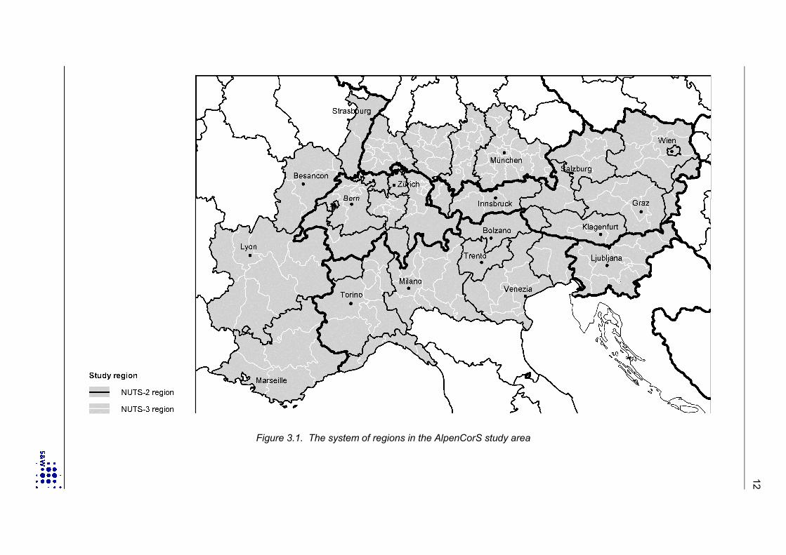
Figure 3.1. The system of regions in the AlpenCorS study area

12

Figure 3.2. The road network in the AlpenCorS study area

13

Figure 3.3. The rail network in the AlpenCorS study area

14

Figure 3.4. Airports in the AlpenCorS study area

15

16

4 Scenarios

This chapter describes the scenarios modelled with the SASI model for AlpenCorS. First, a refer-ence scenario is defined which includes the most important infrastructure projects in Europe butnot the Brenner tunnel. Then six transport infrastructure scenarios are defined to analyse the ef-fects of the Brenner tunnel and other transport infrastructure projects at the intersection of Corri-dors I and V.

4.1 The Reference Scenario (Scenario 000)

The Reference Scenario 000 serves as benchmark for the comparison between policy scenarios.For the reference scenario in AlpenCorS (Scenario 000) a number of assumptions are made:

- For the period between 1981 and 2001, it is assumed for the reference scenario that the rail,road and air networks have developed as they have in reality. This means that new transportinfrastructure projects or upgrades of existing infrastructure, e.g. from national roads to motor-ways, are implemented in the model network database in the year in which they were opened inreality. The same network evolution in the years 1981 to 2001 is also used in all policy scenar-ios, i.e. the policy scenarios differ only from 2001 onwards.

- For the period between 2001 and 2021, it is assumed for the reference scenario that onlytransport infrastructure projects that are part of the new list of TEN priority projects defined bythe European Union (European Commission, 2004) are implemented. However, it is assumedthat the Brenner tunnel, although it is part of the priority projects, is not implemented – this as-sumption was made in order to analyse the effect of the Brenner tunnel separately (in ScenarioAS1, see below). In addition, major railway tunnel projects in Switzerland, which have similarimportance as the TEN priority projects, are included in the reference scenario. The new infra-structure projects are assumed to be implemented in the implementation year published. How-ever, in the past expectations with respect to the implementation schedule of major transportinfrastructure projects have been too optimistic in many cases. No other transport infrastructuredevelopments in Europe are included in the reference scenario. Figure 4.1 shows the TEN pri-ority projects and the major rail projects in Switzerland. Table 4.1 lists these projects and theirmajor links affecting the AlpenCorS study area.

4.2 Infrastructure Scenarios

Besides the reference scenario, six transport infrastructure scenarios were simulated. The firstfive of these were designed to be compatible with the scenarios examined in the Territorial ImpactAnalysis of the Dipartimento di Ingegneria Gestionale of the Politecnico di Milano (Camagni andMusolino, 2003 and Camagni et al., 2004). In addition, a sixth scenario assuming the implemen-tation of the full list of projects envisaged in the TEN and TINA programmes was simulated.

4.2.1 The Brenner Tunnel (Scenario AS1)

Although the Brenner tunnel is part of TEN Priority Project No 1, the rail axis Berlin-Verona/Mila-no-Bologna-Napoli-Messina-Palermao (see Table 4.1), its implementation was not included inReference Scenario 000 in order to analyse it separately. This is done in the first transport infra-structure scenario, Scenario AS1.

Figure 4.1. Transport projects of the Reference Scenario 000 and Scenario AS1 in the AlpenCorS study area

17

18

Table 4.1 TEN priority projects and major Swiss projects in the AlpenCorS study area

No. TEN project Completion date

1 Rail axis Berlin-Verona/Milan-Bologna-Napoli-Messina-Palermo - Munich-Kufstein (2015) - Kufstein-Innsbruck (2009) - Brenner tunnel (2015)* ** - Verona-Naples (2007) - Milan-Bologna (2006)

2006-2015

3 High-speed rail axis of South West Europe - Pvontepellier- Nîmes (2010)

2005-2020

4 TGV Est Paris-Saarbrücken-Mannheim 2007

6 Rail axis Lyon-Trieste/Koper-Ljubljana-Budapest-Ukraine - Lyon-St-Jean-de-Maurienne (2015) - Mont Cenis tunnel (2015-2017)* - Bussoleno-Turin (2011) - Turin-Venice (2010) - Venice-Trieste/Koper-Ljubljana (2015) - Ljubljana-Budapest (2015)

2010-2015

10 Malpesa airport 2001

17 Rail axis Paris-Strasbourg-Stuttgart-Wien-Bratsilava -Baudrecourt-Strasbourg-Stuttgart (2015) - Kehl bridge (2015) - Stuttgart-Ulm (2012) - Munich-Salzburg (2015)* - Salzburg-Vienna (2012) - Vienna-Bratislava (2010)*

2010-2015

22 Rail axis Athens-Sofia-Budapest-Vienna-Prague-Nuremberg - Budapest-Vienna (2010)* - Brno-Prague-Nuremberg (2010)*

2010-2015

23 Rail axis Gdanks-Warsaw-Brno/Bratislava-Vienna - Katowice-Brno-Breclav (2010) - Katowice-Zilina-Nove Misto n.V. (2010)

2010-2015

24 Rail axis Lyon/Genoa-Basel-Buisburg-Rotterdam/Antwerp - Lyon-Mulhouse-Mülheim (2018)* - Genoa-Milan/Novara-Swiss border (2013) - Basel-Karlsruhe (2015)

2009-2010

25 Motorway Gdansk-Brno/Bratislava-Vienna - Gdansk-Katowice (2010) - Katowice-Brno/Zilina (2019* - Brno-Vienna (2009)*

2009-2010

No. Swiss project Completion date

CH1 Gotthard axis- Zimmerberg tunnel (2011)- Gotthard tunnel (2015)- Ceneri tunnel (2015)

2011-2015

CH2 Lötschberg tunnel -2015

* Cross-border link ** The Brenner tunnel was not included in the reference scenario (see text).

19

Because of the importance for the AlpenCorS area and in particular for the Autonomous Provinceof Trento, the assumptions for the Brenner corridor are described in more detail. The Brenner railaxis between München and Verona is the core element of TEN Priority Project No. 1, a rail corri-dor from Berlin via the Alps to southern Italy. Parts of the planned transport infrastructure in thiscorridor is already in operation, e.g. the high-speed rail link between Firenze and Roma, otherparts are under construction or in the planning phase. The Brenner tunnel and its northern andsouthern approaches are key projects to overcome a major transport bottleneck and reduce envi-ronmental effects of transport in Europe.

The Brenner rail corridor and in particular the tunnel was the subject of a large number of feasibil-ity and other studies (for a summary see EURAC-Research et al., 2003). The plan foresees afour-track rail line for the 400 km between München and Verona consisting of two tracks of theexisting line and two new tracks for high-speed passenger and freight services. For the northernand southern approaches to the Brenner tunnel, national transport planning in Italy, Austria andGermany made the necessary decisions to implement the new line. In 2004 a treaty betweenAustria and Italy was signed in which the construction of the Brenner tunnel was concluded.

Similar to many other major transport infrastructure projects, different parts of the Brenner railaxis will become operational at different points in time. Parts of the northern approach in Austriaand related links in Germany giving more capacity to the Brenner axis and the Bozen bypass willbe in operation by the end of this decade. The Brenner tunnel is expected to be in operation by2015 as well as its southern exit south of Franzensfeste and the approach into Verona. TheTrento bypass is expected to be in operation by 2020. However, other links between the Brennertunnel and Verona will probably not be in operation before 2030 (e.g. EURAC-Research, et al.,2003) and are therefore not included in Scenario AS1, but an earlier implementation is assumedin Scenario AS2 (see below).

For passenger transport, the Brenner axis will bring substantial improvements in travel time. Thedesign speed for high-speed trains on the link will be 250 km/h and 200 km/h in the Brenner tun-nel (BBT, 2002a). Rail travel times between München and Verona will go down from 5.5 hourstoday to less than three hours in the future and probably down to 2.5 hours in the far future. TheBrenner tunnel itself will lead to a reduction in rail travel time between Innsbruck and Bozen/Bol-zano from 124 to 50 minutes. It is assumed that high-speed trains will call at the main stations ofMünchen, Innsbruck, Bozen/Bolzano, Trento and Verona (AG Brennerbahn, 2004)

Figure 4.1 shows the part of the Brenner axis upgraded in Scenario AS1. Table 4.2 shows thecurrent travel times of EC trains and, based on the expected implementation years indicatedabove, the SASI model assumptions for future high-speed train travel times between the majorcentres in the corridor assumed for Scenario AS1. These assumptions do not include the furtherreductions on the section between Trento and Verona assumed in Scenario AS2 (see below).

Table 4.2 Current passenger travel times and assumptions for future years (minutes).

From to 2004 2011 2016 2021

München Innsbruck 116 88 70 60

Innsbruck Bozen/Bolzano 124 124 50 50

Bozen Trento 34 30 25 20

Trento Verona 55 55 43 40

München Verona 329 297 188 170

20

However most of the future capacity of the Brenner rail axis will be used for rail freight transport.80 percent of the future capacity of 400 trains will be freight trains. The rail freight capacity will beincreased from 15 million tons per year to 40 million tons per year in order to accommodate theexpected growth in freight transport in the corridor (AG Brennerbahn, 2004). The design speedfor freight trains in the Brenner tunnel will be 100 to 120 km/h for ordinary trains and up to 160km/h for a limited number of express freight trains (BBT, 2002a). Rail freight transport times be-tween München and Verona are currently about ten hours including terminal times and will finallybe reduced to 5 hours.

Important for the modal shift of freight from road to rail are the combined transport terminals ena-bling freight transport chains lorry to freight train to lorry. There are five intermodal transport ter-minals along the Brenner corridor which all have space for capacity extensions (ARGE ALP,2003; BBT, 2002b):

- Verona: Terminal Quadrante Europa- Trento: Interbrennero S.P.A.- Hall in Tirol: TSSU- Wörgl- München-Riem

In addition, there are plans to implement a combined transport terminal in Bozen/Bolzano. For thereference scenario of the SASI model it is assumed that the six combined transport terminals willprovide shuttle services for lorries through the Brenner tunnel. It is assumed that from each com-bined transport terminal on either side of the Brenner tunnel there will be shuttle services to allthree combined transport terminals on the other side of the tunnel, e.g. there will be shuttle serv-ices from Trento to Hall, Wörgl and München.

4.2.2 Southern Rail Bypass (Scenario AS2)

In this scenario it is assumed that, in addition to the implementation of the Brenner tunnel, theItalian part of the Brenner axis south of the Brenner tunnel will be further improved by a series oflong rail tunnels by 2020. In the Provincia Autonoma di Trento this means tunnels between Faedoand Mattarello and again from south of Mattarello to Peri in the Provincia di Verona. These im-provements will allow full separation of freight and passenger transport and make the trans-Alpinerail link more competitive for passengers. It is assumed that the passnger travel times betweenTrento and Verona will go down to 25 minutes until 2021. Figure 4.3 shows the southern rail by-pass. In every other respect Scenario AS2 is identical to Scenario AS1.

4.2.3 Motorways Valdastico and Pedemontana (Scenario AS3)

In this scenario it is assumed that, in addition to the implementation of the Brenner tunnel, thenorthern part of the Italian motorway A31 (Valdastico) will be built. The motorway section is about40 km long. The completed A31 will directly link Trento with Vicenza, allow better separation offreight and passenger transport and will benefit the intermodal freight terminal in Trento. In addi-tion it is assumed that the Pedemontana Veneta motorway will be continued to link Vicenza withTreviso. Both motorway projects will link the north-eastern parts of Italy with the Brenner corridorand northern Europe without the detour via Verona. Figure 4.2 shows the alignment of the Val-dastico and Pedemontana motorways. In every other respect Scenario AS3 is identical to Sce-nario AS1.

21

4.2.4 Valsugana Road and Rail Corridor (Scenario AS4)

In this scenario it is assumed that, in addition to the implementation of the Brenner tunnel, thelevel of service of the Valsugana corridor will be improved. The Valsugana corridor is located eastof Trento and offers an alternative connection from the Brenner corridor to the Veneto region. Themeasures of the scenario aim at improving the safety standards of national road SS 47 and anincrease of travel speed and train frequency and promotion of the intermodal freight terminal inTrento. Figure 4.3 shows the alignment of the Valsugana corridor. In every other respect Sce-nario AS4 is identical to Scenario AS1.

4.2.5 Combination Scenario AS1+AS2+AS3+AS4 (Scenario AS5)

In this scenario it is assumed that, in addition to the implementation of the Brenner tunnel, thethree infrastructure projects examined in scenarios AS2, AS3 and AS4 are implemented together:the southern rail bypass, the Valdastico and Pedemontana motorways and the Valsugana roadand rail corridor. In every other respect Scenario AS5 is identical to Scenario AS1.

4.2.6 Other European Infrastructure Improvements (Scenario AS6)

The current plans for infrastructure development in Europe go far beyond the TEN priority proj-ects included in the reference scenario. It is therefore assumed in this scenario that, besides theimplementation of the Brenner tunnel, the complete TEN and TINA investment programme forroad and rail will be implemented according to realistic assumptions on the year of implementa-tion, including the local transport infrastructure projects as combined in Scenario AS5. This sce-nario will allow to assess both the impacts of local transport infrastructure projects and the im-pacts of more strategic options with a wider European scope. In every other respect ScenarioAS6 is identical to Scenario AS1.

22

Figure 4.2. Further transport infrastructure scenarios (road): Valdastico/Pedemontana (ScenarioAS3) and Valsugana (Scenario AS4)

Figure 4.3. Further transport infrastructure scenarios (rail): Southern rail bypass (Scenario AS2)and Valsugana (Scenario AS4)

23

5 Simulation Results

In this chapter the results of the six transport infrastructure scenarios defined in the previouschapter are reported.

5.1 The Reference Scenario (Scenario 000)

The Reference Scenario 000 as defined in the previous chapter serves as benchmark for thecomparison of the transport infrastructure policy scenarios. Figures 5.1 to 5.16 show selected re-sults of the simulation of the reference scenario with the SASI model.

Figures 5.1 and 5.2 illustrate the temporal and spatial scope of the simulations. All simulationsstart in the year 1981 and continue over 40 years until 2021 in one-year increments. The years2001 to 2021 are the actual forecasting period, as the most recent Europe-wide regional data areof 2001. The years 1981 to 2001 serve to illustrate the development in the past. Each line in thediagram corresponds to one of 34 countries including the 25 present countries of the EuropeanUnion plus Norway and Switzerland and the candidate countries Bulgaria and Romania and thewestern Balkan countries Albania, Bosnia and Herzegowina, Croatia, Makedonia and Yugoslavia.The heavy black line labelled EU represents the average of the 34 countries. The variable GDPper capita is used as an example To exclude the effects of inflation, all GDP-per-capita values areexpressed in Euro of 1998.

Figure 5.1 shows average GDP per capita of all 34 countries. Except the former "cohesion"countries Portugal, Spain and Greece, all old member states of the EU have GDP per capitaabove the European average, whereas all new member states and the Balkan countries haveGDP per capita below the European average. According to the model these differences will per-sist over a long time.

Figure 5.2 shows the same variable, GDP per capita for the 33 AlpenCorS NUTS-2 regions (seeTable 3.1). The letters associated with each line in the diagram indicate the 34 regions:

BL Burgenland NO Niederösterreich VI WienCA Kärnten ST Steiermark OO OberösterreichSB Salzburg TY Tirol VA VorarlbergGE Genève/Lausanne BE Bern BS BaselZU Zürich SG St. Gallen LZ LuzernBA Bellinzona FB Freiburg TB TübingenMU Oberbayern AU Schwaben AL AlsaceFC Franche-Comté RA Rhône-Alpes PA Provence-AlpesPI Piemonte VD Valle d'Aosta LI LiguriaLO Lombardia VE Veneto FV Friuli Venezia GiuliaBO Bolzano TR Trento SI Slovenia

The heavy black line labelled AC represents the average of the AlpenCorS study area. It is obvi-ous that the AlpenCorS region as a whole has a GDP per capita well above the European aver-age. The regions in Switzerland, topped by Zürich, are the most productive and wealthiest Al-penCorS regions, followed by the regions in southern Germany and Austria. The Italian regionsare below the average of the AlpenCorS regions but above the European average. The Autono-mous Province of Trento is among the most productive and most affluent regions of the Italian Al-penCorS regions.

24

Figure 5.1. Reference Scenario 000: GDP per capita (in 1,000 Euro of 1998) by country 1981-2021

Figure 5.2. Reference Scenario 000: GDP per capita (in 1,000 Euro of 1998) by AlpenCorS re-gion 1981-2021 (for explanation of region codes see text)

25

Figures 5.3 and 5.4 show the spatial distribution of GDP per capita in the Reference Scenario 000in the year 2021. In Figure 5.3 the familiar North-South axis of affluence from the Nordic countriesthrough Germany and Switzerland to northern Italy is clearly seen, with the rest of the old EUmember states in the middle range and the new member states and the Balkan countries far be-low. Also the gap in income between urban and rural regions is apparent. Figure 5.4 shows thesame data enlarged for the AlpenCorS regions. Again the top position in GDP per capita of theSwiss regions becomes apparent. The two autonomous provinces of Bolzano and Trento have aGDP per capita of more than 125 percent of the European average.

As in this project the role of transport infrastructure for regional economic development is the fo-cus of attention, Figures 5.5 to 5.12 show the spatial distribution of accessibility. As it was ex-plained in AlpenCorS Deliverable D2.2 (Spiekermann and Wegener, 2004a), four accessibility in-dicators enter the production functions of the SASI model: (i) accessibility by road and rail fortravel (ii) accessibility by road, rail and air for travel, (iii) accessibility by road for freight and (iv)accessibility by road and rail for freight (Schürmann et al., 1997).

The accessibility maps at the European scale (Figures 5.5, 5.7, 5.9 and 5.11) show the decline inaccessibility from the European core in north-western Europe to the peripheral regions in theNordic and Baltic countries, northern England, Scotland and Ireland, the south of France, Spainand Portugal, southern Italy, Greece and the Balkan countries.

The enlarged maps of the AlpenCorS study area (Figures 5.6, 5.8, 5.10 and 5.12) show this inmore detail. In Figure 5.6, which shows combined road and rail accessibility for travel, the high-accessibility road and rail corridors between Torino and Venezia and between Milano and Ge-nova stand out. The Brenner corridor, however, is not visible. In Figure 5.8, which shows thecombination of road, rail and air accessibility, regions with major airports, such as München,Wien, Milano, Zürich and Innsbruck, are highlighted. Accessibility for freight is more spread out asfreight transport is dominated by road and the road network is more dispersed than the rail net-work. Nevertheless, also freight accessibility shows a decline from the countries north of the Alpsto those south of the Alps. This tendency may be sharpened by the fact that the motorway chargerecently introduced on German motorways has not yet been incorporated in the reference sce-nario. Therefore Figure 5.10, which shows only road accessibility for freight, highlights the Alpinedivide, which is even more pronounced in Figure 5.12, which shows combined road and rail ac-cessibility for freight.

Figures 5.13 to 5.16 visualise the same information in three-dimensional form. The comparisonbetween accessibility for travel (Figures 5.13 and 5.14) and accessibility for freight (Figures 5.15and 5.16) confirm that accessibility for travel is more peaked and declines from centre to periph-ery more sharply.

26

Figure 5.3. Reference Scenario 000: GDP per capita (EU27+7=100) in 2021

Figure 5.4. Reference Scenario 000: GDP per capita (EU27+7=100) in the AlpenCorS regions in2021

● Innsbruck● Zürich

● Torino

● Milano

● Lyon

Strasbourg ●

München ●Wien ●

● Ljubljana

● Venezia

● Trento

● Bolzano

27

Figure 5.5. Reference Scenario 000: Accessibility road/rail (travel, million) in 2021

Figure 5.6. Reference Scenario 000: Accessibility road/rail (travel, million) in the AlpenCorS re-gions in 2021


● Torino

● Milano

● Lyon

Strasbourg ●


● Ljubljana

● Venezia

● Trento

● Bolzano

28

Figure 5.7. Reference Scenario 000: Accessibility road/rail/air (travel, million) in 2021

Figure 5.8. Reference Scenario 000: Accessibility road/rail/air (travel, million) in the AlpenCorSregions in 2021


● Torino

● Milano

● Lyon

Strasbourg ●


● Ljubljana

● Venezia

● Trento

● Bolzano

29

Figure 5.9. Reference Scenario 000: Accessibility road (freight, million) in 2021

Figure 5.10. Reference Scenario 000: Accessibility road (freight, million) in the AlpenCorS re-gions in 2021


● Torino

● Milano

● Lyon

Strasbourg ●


● Ljubljana

● Venezia

● Trento

● Bolzano

30

Figure 5.11. Reference Scenario 000: Accessibility road/rail (freight, million) in 2021

Figure 5.12. Reference Scenario 000: Accessibility road/rail (freight, million) in the AlpenCorSregions in 2021


● Torino

● Milano

● Lyon

Strasbourg ●


● Ljubljana

● Venezia

● Trento

● Bolzano

31

Figure 5.13. Reference Scenario 000: Accessibility road/rail (travel, million) in 2021

Figure 5.14. Reference Scenario 000: Accessibility road/rail/air (travel, million) in 2021

32

Figure 5.15. Reference Scenario 000: Accessibility road (freight, million) in 2021

Figure 5.16. Reference Scenario 000: Accessibility road/rail (freight, million) in 2021

33

5.2 Infrastructure Scenarios

In the remainder of this chapter the six infrastructure scenarios examined are presented. Thescenarios are systematically compared in Chapter 6.

5.2.1 Effects of the Brenner Tunnel (Scenario AS1)

Figures 5.17 to 5.26 show the results of the simulation of Scenario AS1, which is in every respectidentical to the Reference Scenario 000 except that it is assumed that the Brenner tunnel and itsnorthern and southern approaches will be completed until 2015 (see Chapter 4).

Because the causal chain in the SASI model goes from accessibility to GDP, first the changes inaccessibility are presented. Because these changes are small, it would not be possible to detectany differences between the "with" and the "without" scenarios by looking at the absolute num-bers Therefore the changes are highlighted by difference maps showing the difference in acces-sibility between Scenario AS1 with the Brenner tunnel and the Reference Scenario 000 withoutthe Brenner tunnel.

Figures 5.17 to 5.24 show these differences for the four accessibility indicators used in the SASImodel. The colour scheme of the difference maps is scaled in a way that light grey indicates nochange, blue a negative difference and red a positive difference. As to be expected, all maps aregrey or red because if the Brenner tunnel is built, all regions are either not affected or experiencea gain in accessibility.

Figures 5.17 to 5.20 show the effect of the Brenner tunnel on accessibility for travel. It can beseen in Figures 5.17 and 5.18, which show the effects of the tunnel on accessibility by road andrail, that the effects are concentrated at the tunnel exits but extend far across the European conti-nent, down the Italian peninsula and in north-eastern direction towards München, Wien and be-yond, but also along the east-west corridor in northern Italy between Milano and Venezia, Corri-dor V. The results are similar if also air travel is considered (Figures 5.19 and 5.20).

Figures 5.21 and 5.22 show the effects of the Brenner tunnel on accessibility for freight by road.Here the effects are even more far-reaching, but now the strongest impacts north of the Alps arein Germany, the Czech Republic and Poland as well as in the Baltic and Nordic states. Remarka-bly, the regions closest to the tunnel exits, Bozen/Bolzano and Innsbruck, are less affected thanthe area around Verona. The reason for this is that from the regions close to the Brenner tunnelthe use of the shuttle trains for carrying lorries through the tunnel is not attractive because of thetime and cost of loading lorries on trains, which makes it attractive only for longer distances, e.g.from München to Verona. Remarkably, regions farther east and west of the Brenner tunnel axisare not affected at all (indicated by the colour grey) as these regions use other Alpine crossings.If, however, also rail is considered as in Figures 5.23 and 5.24, Bozen/Bolzano and Trento havethe strongest gains in accessibility.

Figures 5.25 and 5.26, finally, show how these changes in accessibility affect regional economicdevelopment. Now a different type of difference map is used. This map, too, shows negative dif-ferences in blue and positive differences in red. However, the variable GDP per capita is stan-dardised to the European average (EU27+7=100). This makes it possible that the maps showrelative winners and losers: regions shaded in blue suffer in relative terms if the Brenner tunnel isbuilt; regions shaded in red benefit in relative terms – but both types of regions may grow in ab-solute terms.

34

Figure 5.17. Effect of the Brenner tunnel: Difference in accessibility road/rail (travel, million), be-tween Scenario AS1 and Scenario 000 in 2021 (%)

Figure 5.18. Effect of the Brenner tunnel: Difference in accessibility road/rail (travel, million), be-tween Scenario AS1 and Scenario 000 in the AlpenCorS regions in 2021 (%)


● Torino

● Milano

● Lyon

Strasbourg ●


● Ljubljana

● Venezia

● Trento

● Bolzano

35

Figure 5.19. Effect of the Brenner tunnel: Difference in accessibility road/rail/air (travel, million),between Scenario AS1 and Scenario 000 in 2021 (%)

Figure 5.20. Effect of the Brenner tunnel: Difference in accessibility road/rail/air (travel, million),between Scenario AS1 and Scenario 000 in the AlpenCorS regions in 2021 (%)


● Torino

● Milano

● Lyon

Strasbourg ●


● Ljubljana

● Venezia

● Trento

● Bolzano

36

Figure 5.21. Effect of the Brenner tunnel: Difference in accessibility road (freight, million), be-tween Scenario AS1 and Scenario 000 in 2021 (%)

Figure 5.22. Effect of the Brenner tunnel: Difference in accessibility road (freight, million), be-tween Scenario AS1 and Scenario 000 in the AlpenCorS regions in 2021 (%)


● Torino

● Milano

● Lyon

Strasbourg ●


● Ljubljana

● Venezia

● Trento

● Bolzano

37

Figure 5.23. Effect of the Brenner tunnel: Difference in accessibility road/rail (freight, million),between Scenario AS1 and Scenario 000 in 2021 (%)

Figure 5.24. Effect of the Brenner tunnel: Difference in accessibility road/rail (freight, million),between Scenario AS1 and Scenario 000 in the AlpenCorS regions in 2021 (%)


● Torino

● Milano

● Lyon

Strasbourg ●


● Ljubljana

● Venezia

● Trento

● Bolzano

38

The two maps 5.25 and 5.26 show that, like the effects on accessibility, the effects of the Brennertunnel on regional economic development spread far across the European continent: to the southalong the Italian peninsula, to the north as far as southern Sweden and Norway and to the westalong Corridor V. The regions south of the tunnel, Bozen/Bolzano and Trento, benefit most fromthe implementation of the tunnel followed by Innsbruck and other regions in Tirol as well as insouthern Bavaria and regions around Verona.

However, the map legend tells that these benefits are not very large compared with the changesin accessibility through the tunnel presented in Figures 5.19 to 5.24. As it will be shown later (seeChapter 6), the Trento region can expect to gain 0.76 percent of annual GDP from the Brennertunnel (in 2021). Applied to the GDP forecasts for the region this translates into about 120 millionEuro of 1998 per year for Trento. Translated into Euro of today this would be 175 million in totalor 300 Euro for each inhabitant. Note, however, that these figures relate to 2021. In the years un-til 2021 the benefits are smaller as the effects gradually build up following the implementation ofthe infrastructure.

5.2.2 Effects of other Transport Projects (Scenarios AS2 to AS6)

Figures 5.27 to 5.38 show the impacts of the remaining transport infrastructure scenarios on re-gional economic development.

The first four of these scenarios can be treated en bloc as their results are very similar. In allcases the effects are small but far-reaching in geographical terms. In all scenarios the north-southcorridor from eastern Germany to southern Italy is clearly pronounced and very similar to thespatial pattern of impacts of Scenario AS1 shown in Figures 5.25 and 5.26. In all scenarios, theprovinces south of the Brenner tunnel, Bozen/Bolzano and Trento, benefit most, but in no case bymore than one percent of their GDP. The scenarios which aim at improving the transport networksouth of the Brenner tunnel succeed in spreading the tunnel effects to adjacent regions, in par-ticular to Vicenza, Padova, Belluno, Treviso and Venezia. Scenario AS3 assuming the Valdasticoand Pedemontana motorway extensions is most successful in promoting other regions, whereasScenario AS4 assuming the upgrading of the Valsugana road and rail corridor has more local ef-fects. Not surprisingly Scenario AS5, in which the infrastructure improvements of Scenarios AS2to AS4 are combined, has the strongest effects in spreading the tunnel effects to other Italian re-gions.

The last scenario, AS6, is a special case as it considers, besides the local transport projectscombined in Scenario AS5, also transport infrastructure improvements outside the AlpenCorSarea. Figure 5.35 and 5.36 show that, as to be expected, the effects of these other projects aremuch stronger than those of the local transport projects considered so far. Moreover, because thefocus of these programmes has been recently re-directed towards improving the transport sys-tems of the new EU member states, the largest economic impacts by the projects appear insouthern and eastern Europe. Because of this, large parts of France, Germany, Switzerland andnorth-western Italy become relative losers in economic terms as the new member states take ad-vantage of these improvements in accessibility. However, due to the influence of the Brennertunnel and the associated local transport projects, the provinces of Bolzano and Trento and theirneighbouring regions remain on the winner side.

Figures 5.37 and 5.38 visualise the huge difference in magnitude between the economic effectsof the local projects (as combined in Scenario AS5) and the much larger impacts of the EuropeanTEN and TINA programmes in three-dimensional form drawn to the same vertical scale.

39

Figure 5.25. Effect of the Brenner tunnel: Difference in GDP per capita between Scenario AS1and Scenario 000 in 2021 (%)

Figure 5.26. Effect of the Brenner tunnel: Difference in GDP per capita between Scenario AS1and Scenario 000 in the AlpenCorS regions in 2021 (%)


● Torino

● Milano

● Lyon

Strasbourg ●


● Ljubljana

● Venezia

● Trento

● Bolzano

40

Figure 5.27. Effect of the Brenner tunnel (AS1) plus southern rail bypass: Difference in GDP percapita between Scenario AS2 and Scenario 000 in 2021 (%)

Figure 5.28. Effect of the Brenner tunnel (AS1) plus southern rail bypass: Difference in GDP percapita between Scenario AS2 and Scenario 000 in the AlpenCorS regions in 2021 (%)


● Torino

● Milano

● Lyon

Strasbourg ●


● Ljubljana

● Venezia

● Trento

● Bolzano

41

Figure 5.29. Effect of the Brenner tunnel (AS1) plus Valdastico/Pedemontana: Difference in GDPper capita between Scenario AS3 and Scenario 000 in 2021 (%)

Figure 5.30. Effect of the Brenner tunnel (AS1) plus Valdastico/Pedemontana: Difference in GDPper capita between Scenario AS3 and Scenario 000 in the AlpenCorS regions in 2021 (%)


● Torino

● Milano

● Lyon

Strasbourg ●


● Ljubljana

● Venezia

● Trento

● Bolzano

42

Figure 5.31. Effect of the Brenner tunnel (AS1) plus Valsugana road/rail corridor: Difference inGDP per capita between Scenario AS4 and Scenario 000 in 2021 (%)

Figure 5.32. Effect of the Brenner tunnel (AS1) plus Valsugana road/rail corridor: Difference inGDP per capita between Scenario AS4 and Scenario 000 in the AlpenCorS regions in 2021 (%)


● Torino

● Milano

● Lyon

Strasbourg ●


● Ljubljana

● Venezia

● Trento

● Bolzano

43

Figure 5.33. Effect of the Brenner tunnel (AS1) plus AS2+AS3+AS4: Difference in GDP per cap-ita between Scenario AS5 and Scenario 000 in 2021 (%)

Figure 5.34. Effect of the Brenner tunnel (AS1) plus AS2+AS3+AS4: Difference in GDP per cap-ita between Scenario AS5 and Scenario 000 in the AlpenCorS regions in 2021 (%)


● Torino

● Milano

● Lyon

Strasbourg ●


● Ljubljana

● Venezia

● Trento

● Bolzano

44

Figure 5.35. Effect of all TEN and TINA road and rail projects: Difference in GDP per capita be-tween Scenario AS6 and Scenario 000 in 2021 (%)

Figure 5.36. Effect of all TEN and TINA road and rail projects: Difference in GDP per capita be-tween Scenario AS6 and Scenario 000 in the AlpenCorS regions in 2021 (%)


● Torino

● Milano

● Lyon

Strasbourg ●


● Ljubljana

● Venezia

● Trento

● Bolzano

45

Figure 5.37. Effect of the Brenner tunnel plus AS2+AS3+AS4: Difference in GDP per capita be-tween Scenario AS5 and Scenario 000 in 2021

Figure 5.38. Effect of all TEN and TINA road and rail projects: Difference in GDP per capita be-tween Scenario AS6 and Scenario 000 in 2021

46

6 Scenario Comparison

The tables on the following pages compare the results of the six transport infrastructure scenarioswith the Reference Scenario 000 in the target year 2021.

The model results were aggregated from the 186 NUTS-3 regions in the AlpenCorS area to the33 NUTS-2 regions in the area and to the AlpenCorS area as a whole. This aggregation providesalso information on the provinces of Bozen/Bolzano and Trento as these two regions are bothNUTS-2 and NUTS-3 regions.

In each table the first column contains the simulation results in the Reference Scenario 000 forthe target year 2021. The remaining six columns of each table contain differences between thecorresponding results of the six transport infrastructure scenarios and the results of the Refer-ence Scenario 000 in percent of the value in the first column.

Accessibility

Tables 6.1 to 6.4 show the effects of the seven scenarios on the four accessibility indicators usedin the SASI model in the year 2021. Tables 6.1 and 6.2 show the effects of the scenarios on ac-cessibility for travel by road and rail (Table 6.1) and by road, rail and air (Table 6.2). Tables 6.3and Table 6.4 show the effects of the scenarios on accessibility for freight by road (Table 6.3) androad and rail (Table 6.4).

The first column in each table shows the distribution of accessibility in the AlpenCorS regions inReference Scenario 000 in the year 2021 aggregated to NUTS-2 regions. The original NUTS-3values were presented in map form in Figures 5.5 to 5.12. The numbers confirm that the regionsnorth of the Alps have higher accessibility values because they are close to the large agglomera-tions in north-west Europe. Southern Germany and Switzerland have the highest accessibilityvalues followed by the Austrian and Italian regions; however, there are considerable differencesbetween urban and rural regions in each country.

The remaining columns show the effects of the six transport infrastructure scenarios on regionalaccessibility as differences between policy scenario and Reference Scenario 000 in 2021:

In all scenarios all types of accessibility are improved in all regions. This is not surprising becauseonly transport infrastructure improvements were examined. The Brenner tunnel (Scenario AS1) isthe project with the largest effect of the Scenarios AS1 to AS5. The implementation of the tunnelincreases accessibility at its southern end, in the regions of Bozen/Bolzano and Trento, by about4 % and at its northern end, in Tirol, by about 3 %. The effects in Scenarios AS2 to AS5 are al-ways stronger than those of Scenario AS1 because the Brenner tunnel is included in all otherscenarios except the reference scenario. However, the improvements through the additionaltransport infrastructure projects are small. The largest additional effects are due to the southernrail bypass between Trento and Verona (Scenario AS2), the additional effect is no more than onequarter of the initial effect of the tunnel. The additional effects of the two regional transport infra-structure projects, the extension of the Valdastico and Pedemontana motorways (Scenario AS3)and the upgrading of the Valsugana road and rail corridor (Scenario AS4), are much smaller.However, these projects are important for the nearby regions Vicenza and Padova and to a lesserextent Belluno, Treviso and Venezia, because they link these regions better to the tunnel. Theeffect of the Valsugana road and rail corridor (Scenario AS4) is smaller than that of the Valdasticoand Pedemontana motorway extensions (Scenario AS3).

47

-able 6.1. Accessibility road/rail (travel, million)

Difference between policy scenario andReference Scenario 000 in 2021 (%)Region

ReferenceScenario

000in 2021 AS1 AS2 AS3 AS4 AS5 AS6

A BL Burgenland 80.6 +0.03 +0.03 +0.09 +0.03 +0.10 +10.1NO Niederösterreich 85.2 +0.60 +0.74 +0.63 +0.61 +0.77 +10.5VI Wien 93.5 +0.37 +0.57 +0.41 +0.38 +0.60 +11.4CA Kärnten 79.4 +0.02 +0.02 +0.07 +0.02 +0.07 +12.4ST Steiermark 80.9 +0.03 +0.05 +0.07 +0.03 +0.09 +11.9OO Oberösterreich 89.2 +1.64 +1.93 +1.67 +1.66 +1.95 +9.73SB Salzburg 89.5 +1.93 +2.26 +1.96 +1.95 +2.29 +7.70TY Tirol 91.1 +2.59 +3.01 +2.67 +2.62 +3.08 +7.60VA Vorarlberg 94.0 +0.75 +0.92 +0.83 +0.77 +0.99 +5.88

CH GE Genève/Lausanne 88.1 +0.14 +0.17 +0.15 +0.14 +0.17 +5.45BE Bern 90.7 +0.19 +0.19 +0.20 +0.19 +0.20 +4.88BS Basel 99.9 +0.19 +0.19 +0.20 +0.19 +0.20 +4.12ZU Zürich 97.6 +0.21 +0.21 +0.25 +0.22 +0.25 +4.15SG St. Gallen 91.2 +0.19 +0.20 +0.25 +0.19 +0.26 +4.65LZ Luzern 94.3 +0.17 +0.18 +0.18 +0.17 +0.19 +4.02BA Bellinzona 86.9 +0.21 +0.32 +0.21 +0.21 +0.33 +5.46

DE FB Freiburg 100.1 +0.05 +0.05 +0.06 +0.05 +0.06 +4.29TB Tübingen 97.5 +0.32 +0.41 +0.38 +0.33 +0.47 +5.07MU Oberbayern 99.4 +1.59 +1.90 +1.66 +1.62 +1.96 +6.70AU Schwaben 98.8 +0.98 +1.16 +1.05 +1.00 +1.22 +5.86

FR AL Alsace 98.8 +0.03 +0.03 +0.03 +0.03 +0.04 +4.19FC Franche-Comté 88.4 +0.10 +0.10 +0.10 +0.10 +0.11 +4.62RA Rhône-Alpes 81.9 +0.18 +0.29 +0.18 +0.19 +0.29 +5.78PA Provence-Alpes 65.5 +0.28 +0.40 +0.30 +0.28 +0.42 +8.58

IT PI Piemonte 85.2 +0.67 +0.90 +0.70 +0.69 +0.93 +6.69VD Valle d'Aosta 79.2 +0.49 +0.66 +0.51 +0.50 +0.68 +8.69LI Liguria 83.5 +0.70 +0.94 +0.74 +0.72 +0.98 +7.36LO Lombardia 91.2 +0.84 +1.08 +0.88 +0.86 +1.12 +6.72VE Veneto 86.2 +1.18 +1.42 +2.06 +1.25 +2.27 +8.86FV Friuli Venezia Giulia 82.6 +0.19 +0.27 +0.42 +0.19 +0.49 +9.02BO Bolzano 83.2 +4.45 +5.31 +4.66 +4.52 +5.52 +9.76TR Trento 83.7 +3.81 +4.77 +4.34 +3.88 +5.29 +9.70

SI SI Slovenia 79.1 +0.03 +0.05 +0.05 +0.03 +0.07 +10.0

AC AlpenCorS 87.8 +0.66 +0.82 +0.75 +0.67 +0.91 +6.94

48

Table 6.2. Accessibility road/rail/air (travel, million)


ReferenceScenario







SI SI Slovenia 81.0 +0.03 +0.05 +0.05 +0.03 +0.06 +9.25

AC AlpenCorS 90.6 +0.60 +0.74 +0.69 +0.61 +0.83 +6.13

49

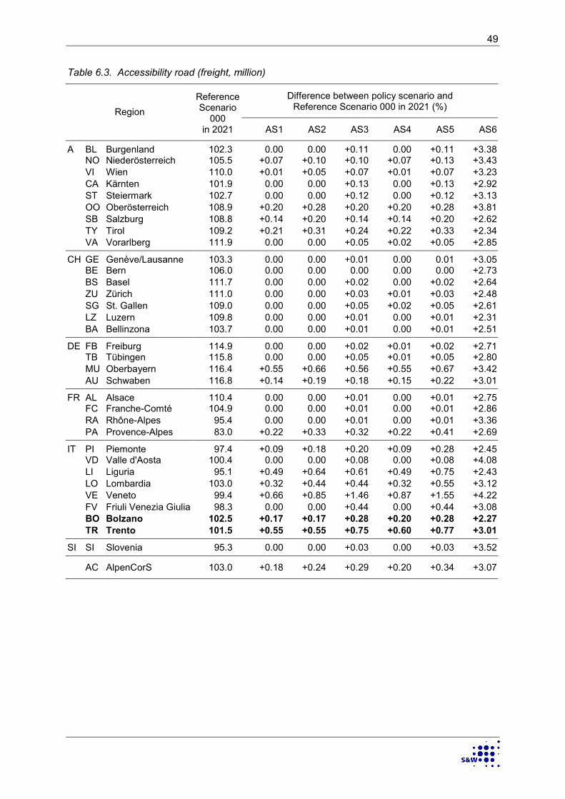
Table 6.3. Accessibility road (freight, million)


ReferenceScenario


A BL Burgenland 102.3 0.00 0.00 +0.11 0.00 +0.11 +3.38NO Niederösterreich 105.5 +0.07 +0.10 +0.10 +0.07 +0.13 +3.43VI Wien 110.0 +0.01 +0.05 +0.07 +0.01 +0.07 +3.23CA Kärnten 101.9 0.00 0.00 +0.13 0.00 +0.13 +2.92ST Steiermark 102.7 0.00 0.00 +0.12 0.00 +0.12 +3.13OO Oberösterreich 108.9 +0.20 +0.28 +0.20 +0.20 +0.28 +3.81SB Salzburg 108.8 +0.14 +0.20 +0.14 +0.14 +0.20 +2.62TY Tirol 109.2 +0.21 +0.31 +0.24 +0.22 +0.33 +2.34VA Vorarlberg 111.9 0.00 0.00 +0.05 +0.02 +0.05 +2.85

CH GE Genève/Lausanne 103.3 0.00 0.00 +0.01 0.00 0.01 +3.05BE Bern 106.0 0.00 0.00 0.00 0.00 0.00 +2.73BS Basel 111.7 0.00 0.00 +0.02 0.00 +0.02 +2.64ZU Zürich 111.0 0.00 0.00 +0.03 +0.01 +0.03 +2.48SG St. Gallen 109.0 0.00 0.00 +0.05 +0.02 +0.05 +2.61LZ Luzern 109.8 0.00 0.00 +0.01 0.00 +0.01 +2.31BA Bellinzona 103.7 0.00 0.00 +0.01 0.00 +0.01 +2.51

DE FB Freiburg 114.9 0.00 0.00 +0.02 +0.01 +0.02 +2.71TB Tübingen 115.8 0.00 0.00 +0.05 +0.01 +0.05 +2.80MU Oberbayern 116.4 +0.55 +0.66 +0.56 +0.55 +0.67 +3.42AU Schwaben 116.8 +0.14 +0.19 +0.18 +0.15 +0.22 +3.01

FR AL Alsace 110.4 0.00 0.00 +0.01 0.00 +0.01 +2.75FC Franche-Comté 104.9 0.00 0.00 +0.01 0.00 +0.01 +2.86RA Rhône-Alpes 95.4 0.00 0.00 +0.01 0.00 +0.01 +3.36PA Provence-Alpes 83.0 +0.22 +0.33 +0.32 +0.22 +0.41 +2.69

IT PI Piemonte 97.4 +0.09 +0.18 +0.20 +0.09 +0.28 +2.45VD Valle d'Aosta 100.4 0.00 0.00 +0.08 0.00 +0.08 +4.08LI Liguria 95.1 +0.49 +0.64 +0.61 +0.49 +0.75 +2.43LO Lombardia 103.0 +0.32 +0.44 +0.44 +0.32 +0.55 +3.12VE Veneto 99.4 +0.66 +0.85 +1.46 +0.87 +1.55 +4.22FV Friuli Venezia Giulia 98.3 0.00 0.00 +0.44 0.00 +0.44 +3.08BO Bolzano 102.5 +0.17 +0.17 +0.28 +0.20 +0.28 +2.27TR Trento 101.5 +0.55 +0.55 +0.75 +0.60 +0.77 +3.01

SI SI Slovenia 95.3 0.00 0.00 +0.03 0.00 +0.03 +3.52

AC AlpenCorS 103.0 +0.18 +0.24 +0.29 +0.20 +0.34 +3.07

50

Table 6.4. Accessibility road/rail (freight, million)


ReferenceScenario







SI SI Slovenia 118.5 +0.02 +0.03 +0.03 +0.02 +0.04 +5.34

AC AlpenCorS 130.6 +0.55 +0.67 +0.60 +0.56 +0.72 +4.36

51

Scenarios AS5 and AS6 show the effects of policy combinations. In Scenario AS5 it is assumedthat not only the Brenner tunnel and its access links are built (Scenario AS1) but that also thesouthern rail bypass between Trento and Verona is completed (Scenario AS2), the Valdasticoand Pedemontana motorways are extended (Scenario AS3) and the Valsugana road and rail cor-ridor is upgraded (Scenario AS4). In Scenario AS6 all these infrastructure improvements are ex-amined together with the implementation of all presently discussed TEN and TINA road and railproject all over Europe.

As expected, the effects on accessibility of Scenario AS5 are larger than those of all previousscenarios including Scenario AS1. This seems to speak in favour of implementing all infrastruc-ture projects included in Scenario AS5, i.e. in Scenarios AS1 to AS4. But is this justified? Are allthese projects necessary to achieve the desired improvement in accessibility? Do the projectscomplement one another? This is the synergy question. Synergies between policies exist if thesum of their individual effects is smaller than the total effect of their combined implementation in apolicy package. Table 6.5 examines this question using the region of Trento as an example.

Table 6.5. Effects of infrastructure projects on accessibility of Trento

Effects of scenarios (%)

Additional effectAccessibilityEffect

AS1 AS2 AS3 AS4 TotalEffect

AS5 Synergy

Road/rail (travel) +3.81 +0.96 +0.53 +0.07 +5.37 +5.29 –0.08

Road/rail/air (travel) +3.51 +0.90 +0.48 +0.07 +4.96 +4.89 –0.07

Road (freight) +0.55 0.00 +0.20 +0.05 +0.80 +0.77 –0.03

Road/rail (freight) +3.15 +0.38 +0.12 +0.05 +3.70 +3.64 –0.06

The table shows the effects on accessibility of Scenarios AS1 to AS5 for Trento. As the Brennertunnel (Scenario AS1) is included in Scenarios AS2 to AS4, only additional effects of these sce-narios (after subtracting the effects of AS1) are listed. The last column compares the total of theeffects of Scenario AS1 plus the additional effects of Scenarios AS2 to AS4 with the effect of theircombined application in Scenario AS5. For all four types of accessibility the effect of ScenarioAS5 is less than the total of the effects of Scenarios AS1 to AS4, i.e. their synergy is negative.The conclusion is that the Valdastico and Pedemontana motorway extensions (Scenario AS3)and the Valsugana road and rail corridor upgrading (Scenario AS4) partly achieve the same resultin different ways. This does not exclude that they have important local effects in the regionsthrough which they pass and adjacent regions. There may also be good reasons to upgrade theValsugana rail line for environmental reasons, i.e. in order to reduce road traffic in the valley.

Scenario AS6 shows the changes in accessibility that could be expected from the implementationof all TEN and TINA projects in Europe, including those in Scenarios AS1 to AS5. The effects areby an order of magnitude larger than those of the regional and local projects in the other scenar-ios, even though the main emphasis of the TEN and TINA programmes are on the new memberstates in eastern Europe. Even for the regions close to the Brenner tunnel, which benefit mostfrom the tunnel, the effects on accessibility are about twice as large. This demonstrates that in thelong run European developments in transport infrastructure may be more important than localtransport infrastructure improvements.

52

GDP per capita

Tables 6.6 to 6.8 show the effects of the seven scenarios on regional GDP: Table 6.6 on total re-gional GDP, Table 6.7 on GDP per capita Euro of 1998 and Table 6.8 on GDP per capita in per-cent of the European average (EU27+7=100).

The first column in each table shows the distribution of GDP or GDP per capita in the AlpenCorSregions in Reference Scenario 000 in the year 2021 aggregated to NUTS-2 regions. The originalNUTS-3 values of GDP per capita in 1,000 Euro of 1998 were presented in the diagram of Figure5.2. The original NUTS-3 values of GDP per capita (EU27+7=100) were presented in map form inFigures 5.3 and 5.4. The numbers confirm that the AlpenCorS region as a whole has a GDP percapita well above the European average, that the regions in Switzerland, topped by Zürich, arethe most productive and wealthiest AlpenCorS regions, followed by the regions in southern Ger-many and Austria, that the Italian regions are below the average of the AlpenCorS regions butabove the European average, and that the Autonomous Province of Trento is among the mostproductive and most affluent regions of the Italian AlpenCorS regions.

The remaining columns show the effects of the six transport infrastructure scenarios on regionalGDP as differences between policy scenario and Reference Scenario in 2021. The originalNUTS-3 values underlying these NUTS-2 aggregates were presented in map form and as 3Dsurfaces in Figures 5.25 to 5.38.

Table 6.6 presents the results of the GDP forecasts in absolute terms, expressed in Euro of 1998.Not surprisingly, all differences are positive, i.e. all regions experience a gain in production andaffluence due to the transport infrastructure improvements examined. However, the gains aremuch smaller than the gains in accessibility presented in Tables 6.1 to 6.4, and even in the re-gions close to the tunnel do not exceed one percent except in the two scenarios combining sev-eral transport infrastructure projects, Scenarios AS5 and AS6. As in the case of accessibility, theeffects of the European projects outside the AlpenCorS area are much stronger than those of thelocal projects of Scenarios AS2 to AS5, even for the regions close to the Brenner tunnel.

Table 6.7 shows the effects on regional GDP per capita. Here, too, the unit is Euro of 1998, whichmeans that only gains in GDP per capita are recorded. Again the regions near the Brenner axisare most affected, most notably Bozen/Bolzano and Trento, and the much larger effects associ-ated with Scenario AS6 are notable. The relative gains in GDP per capita are slightly smaller thanfor total GDP in Table 6.6 because economically successful regions attract migrants from otherregions and so have to allocate their GDP to more people.

Table 6.8 shows the same indicator, GDP per capita, but standardised to the European average,i.e. the weighted average of all regions in the European Union plus Norway and Switzerland andBulgaria, Romania and the western Balkan countries (EU27+7=100). Now also negative differ-ences appear, i.e. relative winners (with positive differences) and relative losers (with negativedifferences) can be distinguished. As noted in the discussion of individual scenarios in Chapter 5,the positive effects are spread out along a north-south corridor at both ends of the Brenner axis.The effects of Scenario AS6 are now much smaller, as many of the regions in central Europe, in-cluding Swiss, German and most French regions in the AlpenCorS area, become relative losers.However, the regions close to the Brenner tunnel remain on the winner side. If the six transportinfrastructure scenarios are compared, the effects of all six scenarios on the relative position ofthe regions are very similar. For the provinces of Bozen/Bolzano and Trento, for instance, thecombination of the Brenner tunnel with additional projects brings only little extra benefit, exceptwhere all three infrastructure measures, the southern rail bypass, the Valdastico and Pedemon-tana motorways and the Valsugana road and rail corridor, are combined (Scenario AS5).

53

Table 6.6. GDP (Billion Euro of 1998)


ReferenceScenario







SI SI Slovenia 30.8 +0.01 +0.01 +0.01 +0.01 +0.01 +1.70

AC AlpenCorS 2,521.0 +0.11 +0.14 +0.13 +0.12 +0.15 +1.14

54

Table 6.7. GDP per capita (1,000 Euro of 1998)


ReferenceScenario







SI SI Slovenia 17.4 +0.01 +0.01 +0.01 +0.01 +0.01 +1.69

AC AlpenCorS 41.4 +0.11 +0.14 +0.13 +0.12 +0.15 +1.14

55

Table 6.8. GDP per capita (EU27+7=100)


ReferenceScenario


A BL Burgenland 116.8 -0.04 -0.05 -0.03 -0.04 -0.04 +0.43NO Niederösterreich 131.5 +0.05 +0.06 +0.05 +0.05 +0.06 +0.64VI Wien 216.9 +0.02 +0.04 +0.03 +0.03 +0.04 +0.80CA Kärnten 141.4 -0.04 -0.05 -0.04 -0.04 -0.05 +0.84ST Steiermark 145.3 -0.04 -0.05 -0.04 -0.04 -0.04 +0.73OO Oberösterreich 160.5 +0.16 +0.19 +0.16 +0.17 +0.19 +0.24SB Salzburg 179.2 +0.26 +0.29 +0.26 +0.26 +0.29 +0.15TY Tirol 166.2 +0.36 +0.41 +0.37 +0.36 +0.42 +0.14VA Vorarlberg 167.9 +0.06 +0.07 +0.06 +0.06 +0.07 –0.21

CH GE Genève/Lausanne 220.9 -0.03 -0.04 -0.03 -0.03 -0.04 –0.07BE Bern 181.3 -0.02 -0.03 -0.02 -0.02 -0.03 –0.19BS Basel 248.6 -0.02 -0.03 -0.03 -0.02 -0.04 –0.35ZU Zürich 280.4 -0.02 -0.03 -0.02 -0.02 -0.03 –0.38SG St. Gallen 191.9 -0.02 -0.03 -0.01 -0.02 -0.02 –0.28LZ Luzern 213.4 -0.02 -0.03 -0.03 -0.02 -0.04 –0.37BA Bellinzona 173.8 -0.01 -0.01 -0.02 -0.01 -0.01 –0.11

DE FB Freiburg 147.8 -0.04 -0.05 -0.04 -0.04 -0.05 –0.37TB Tübingen 152.3 +0.01 +0.01 +0.01 +0.01 +0.02 –0.26MU Oberbayern 223.9 +0.19 +0.22 +0.20 +0.20 +0.23 –0.08AU Schwaben 148.0 +0.10 +0.12 +0.11 +0.10 +0.12 –0.16

FR AL Alsace 135.7 -0.05 -0.06 -0.05 -0.05 -0.06 –0.35FC Franche-Comté 121.9 -0.04 -0.05 -0.04 -0.04 -0.05 –0.30RA Rhône-Alpes 133.9 -0.03 -0.02 -0.03 -0.03 -0.03 –0.09PA Provence-Alpes 121.7 0.00 0.00 0.00 0.00 0.00 +0.34

IT PI Piemonte 120.9 +0.08 +0.10 +0.08 +0.08 +0.10 +0.03VD Valle d'Aosta 127.5 +0.05 +0.07 +0.05 +0.05 +0.07 +0.54LI Liguria 109.4 +0.10 +0.13 +0.10 +0.10 +0.13 +0.31LO Lombardia 138.0 +0.10 +0.13 +0.11 +0.10 +0.14 –0.01VE Veneto 121.9 +0.19 +0.23 +0.34 +0.20 +0.37 +0.53FV Friuli Venezia Giulia 116.8 -0.01 +0.00 +0.03 -0.01 +0.04 +0.49BO Bolzano 148.4 +0.79 +0.91 +0.82 +0.80 +0.94 +0.76TR Trento 126.8 +0.70 +0.85 +0.79 +0.72 +0.94 +0.79

SI SI Slovenia 63.3 -0.04 -0.05 -0.04 -0.05 -0.05 +0.60

AC AlpenCorS 150.7 +0.06 +0.07 +0.07 +0.06 +0.09 +0.05

56

This leads again to the issue of synergies between the transport infrastructure projects. In Table6.9 the analysis of synergies between scenarios performed for accessibility in Table 6.5 is re-peated for the three GDP indicator presented in Tables 6.6 to 6.8.

Table 6.9. Effects of infrastructure projects on regional GDP of Trento

Effects of scenarios (%)

Additional effectGDPEffect

AS1 AS2 AS3 AS4 TotalEffect

AS5 Synergy

GDP +0.76 +0.16 +0.10 +0.02 +1.04 +1.02 –0.02

GDP/capita (Euro) +0.75 +0.16 +0.10 +0.02 +1.03 +1.00 –0.03

GDP/capita (EU27+7=100) +0.70 +0.15 +0.09 +0.02 +0.96 +0.94 –0.02

The table shows that also with respect to GDP or GDP per capita there are no positive synergiesbetween the infrastructure projects examined. The negative synergies in the last column indicatethat the infrastructure projects, the southern rail bypass, the Valdastico and Pedemontanamotorway extensions (Scenario AS3) and the Valsugana road and rail corridor upgrading (Sce-nario AS4) are at least in part substitutable as they achieve the same gain in GDP per capita forTrento by different means. However, this does not imply that these projects should not be imple-mented. They may have important local effects for the regions through which they pass and adja-cent regions. There may also be good reasons to upgrade the Valsugana rail line for environ-mental reasons, i.e. in order to reduce road traffic in the valley.

To be on the safe side, the synergy analysis performed for accessibility and GDP for the region ofTrento was also performed for all other regions of the AlpenCorS area. The analysis showed thatonly in very few regions positive synergies between the transport infrastructure projects examinedappeared, and that these synergies were very small. The results are therefore not reproduced indetail here.

57

7 Territorial Cohesion

The results of the scenario simulations presented so far have shown how transport infrastructureinvestments improve the accessibility and hence economic competitiveness of regions. However,the transport policy of the European Union does not only serve competitiveness objectives. TheEuropean Union hopes to contribute by its transport policy also to territorial cohesion, a reductionof economic disparities between the central and peripheral regions in Europe. In particular afterthe enlargement of the European Union the great disparities in accessibility between the old andnew member states pose serious problems of spatial equity, which are aggravated by the goalconflict between territorial cohesion and the competitiveness goal of the Lisbon strategy.

In this chapter it will be asked whether the implementation of the transport infrastructure projectsexamined will contribute to convergence or divergence of accessibility and economic develop-ment between the regions in Europe at large and in the AlpenCorS regions.

There are many possible ways to measure the cohesion effects of transport infrastructure proj-ects. The most frequently applied indicators, the coefficient of variation and the Gini coefficient(see Bröcker et al., 2004a), measure the relative variation of regional values around their aver-age. However, relative cohesion indicators hide the fact that if every region gains in income byten percent, the richer regions receive far more than the poorer regions in absolute terms. Whenassessing transport infrastructure projects, it is therefore useful to consider both, relative and ab-solute measures of cohesion. If, for instance, as a consequence of a transport project a rich and apoor region gained both ten percent in GDP per capita, relative cohesion indicators indicate nei-ther convergence nor divergence; however, in absolute terms the rich region would gain muchmore than the poor region. It is even possible that a region is a winner in relative terms but a loserin absolute terms.

Following a suggestion by Bröcker (Bröcker et al., 2004a) one relative and one absolute cohesionindicator are used in the analysis presented here:

- Correlation between relative change and level. This indicator examines the relationship be-tween the change of an indicator and its magnitude by calculating the correlation coefficientbetween them. If for instance the correlation between the changes in GDP per capita in percentand the levels of GDP per capita in a set of regions is positive, the more affluent regions in theset gain more in relative terms than the poorer regions and disparities in income increase. If thecorrelation is negative, the poorer regions gain more in relative term than the richer regions anddisparities decrease.

- Correlation between absolute change and level. This indicator is constructed as the previousone except that absolute changes are considered. This indicator will indicate convergence onlyif the poorer regions gain more not only in relative but also in absolute terms, which is a muchmore stringent definition.

The different results produced by the two indicators are presented first for Scenario AS6, in whichit is assumed that all TEN and TINA projects are implemented. Figure 7.1 shows four scatter dia-grams visualising the correlation between change and level for accessibility and GDP per capitafor the 1,330 regions in Europe forecast in the SASI model. Accessibility is here the total of thefour accessibility indicators presented in Tables 6.1 to 6.4, and GDP per capita is GDP per capitain Euro of 1998 as in Table 6.7.

58

Figure 7.1. Effects of all TEN and TINA projects (Scenario AS6): relative convergence and ab-solute divergence in accessibility (top) and GDP/capita (bottom), all European regions

59

The two diagrams at the top of Figure 7.1 show the correlation between change and level of ac-cessibility. The left diagram shows the correlation between relative change in accessibility andlevel of accessibility, where the term "relative change" indicates the percent difference in regionalaccessibility between Scenario AS6 and the reference scenario in 2021. It can be seen that thegreatest changes in accessibility occur in the left half of the diagram, i.e. in the peripheral regionswith lower accessibility. Hence the regression line slopes downward, and the coefficient of corre-lation r is negative. The right diagram shows the same data but now change in accessibility isplotted in absolute terms. Now the largest gains in accessibility occur in the right half of the dia-gram, i.e. in the central regions with high accessibility. Hence the regression line slopes upwards,and the coefficient of correlation is positive.

The two diagrams at the bottom Figure 7.1 show the correlation between change in GDP percapita and level of GDP per capita. The left diagram shows the correlation between relativechange in GDP per capita and level of GDP per capita, where the term "relative change" indicatesthe percent difference in regional GDP per capita between Scenario AS6 and the reference sce-nario in 2021. It can be seen that the greatest changes in GDP per capita occur in the left half ofthe diagram, i.e. in the poorer regions, in particular the regions in the new member states. Hencethe regression line slopes downward, and the coefficient of correlation r is negative. The rightdiagram shows the same data but now change in GDP per capita is plotted in absolute terms.Now the largest gains in GDP per capita occur in the right half of the diagram, i.e. in the richer re-gions. Hence the regression line slopes upwards, and the coefficient of correlation is positive.

In conclusion, the implementation of the vast infrastructure programme assumed in Scenario AS6would result in convergence in both accessibility and GDP per capita in relative terms. However,in absolute terms, divergence would occur, i.e. the central regions with already high accessibilityand GDP per capita would gain most.

Figure 7.2 shows the results of the same analysis for Scenario AS1, the Brenner tunnel scenario.Now the results are different: there is divergence also in relative terms. This is, however, not sur-prising because the regions gaining most from the Brenner tunnel are located in the centre ofEurope and have above-average GDP per capita. The diagrams clearly show the large gains inaccessibility and GDP per capita in the regions near the Brenner tunnel, Bozen/Bolzano, Trento,Verona and Innsbruck. As a rule, negative cohesion effects can be expected if a major transportinfrastructure project is implemented in an area of already high accessibility.

This result is even more pronounced if the analysis is restricted to the 186 regions in the Alpen-CorS area (Figure 7.3). Clearly the regions close to the tunnel exits, Bozen/Bolzano, Trento,Verona and Innsbruck, are gaining most in accessibility and GDP per capita, whereas other re-gions, particularly in Switzerland, are hardly affected. It must be concluded that the Brenner tun-nel favours only few regions in the AlpenCorS area and so increases the existing imbalances inthe area.

Do the remaining scenarios, in which additional local infrastructure projects are examined, coun-terbalance this divergence? Table 7.1 shows the cohesion effects of all six modelled scenarios interms of relative and absolute coefficients of correlation between change and level of accessibilityand GDP per capita for all European regions and for the regions in the AlpenCorS area. It can beseen that the additional effects of the local projects examined in Scenarios AS2 to AS4 are small.Scenarios AS3 (Brenner tunnel plus Valdastico/Pedemontana motorways) and Scenario AS5(Brenner tunnel plus all local projects) are successful in spreading the tunnel effects to adjacentregions so that at least relative convergence between the AlpenCorS regions occurs, though inabsolute terms the regions near the tunnel exits continue to gain most.

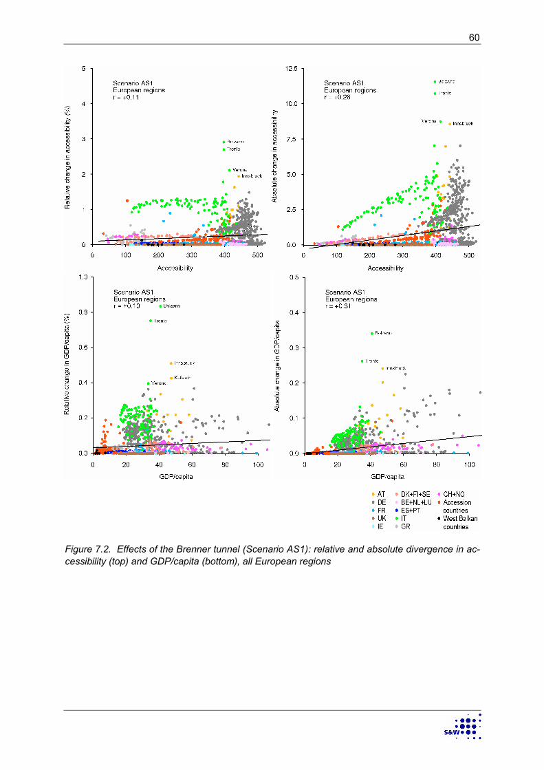
60

Figure 7.2. Effects of the Brenner tunnel (Scenario AS1): relative and absolute divergence in ac-cessibility (top) and GDP/capita (bottom), all European regions

61

Figure 7.3. Effects of the Brenner tunnel (Scenario AS1): relative and absolute divergence in ac-cessibility (top) and GDP/capita (bottom), AlpenCorS regions

62

Table 7.1. Territorial cohesion effects

Coefficient of correlation between change and level

All European regions AlpenCorS regions

Accessibility GDP/capita Accessibility GDP/capita

rel abs rel abs rel abs rel abs

AS1 Brenner tunnel +0.11 +0.26 +0.10 +0.31 +0.12 +0.18 +0.03 +0.38AS2 AS1+rail bypass +0.11 +0.26 +0.09 +0.31 +0.10 +0.17 +0.01 +0.37AS3 AS1+Valdastico +0.12 +0.27 +0.11 +0.31 +0.07 +0.13 –0.01 +0.33AS4 AS1+Valsugana +0.11 +0.27 +0.10 +0.31 +0.11 +0.18 +0.02 +0.38AS5 AS1+AS2+AS3+AS4 +0.12 +0.27 +0.09 +0.31 +0.06 +0.12 –0.02 +0.33AS6 All TEN and TINA –0.34 +0.44 –0.53 +0.67 –0.42 –0.06 –0.29 +0.64

– Convergence + Divergence

63

8 Conclusions

The analysis of different strategies for developing the transport infrastructure of the Brenner corri-dor near its intersection with Corridor V has shown that the implementation of the Brenner tunnelwill be a key factor for linking northern and southern Europe. The spatial effects of the Brennertunnel will be far reaching from the Baltic to the Mediterranean.

The effect of the Brenner tunnel on accessibility for travel extends far across the European conti-nent, down the Italian peninsula and in north-eastern direction towards München, Wien and be-yond, but also along the east-west corridor in northern Italy, Corridor V. The regions south of thetunnel, Bozen/Bolzano and Trento, have the largest gain in accessibility The effects of the tunnelon accessibility for freight are even more far-reaching, with the strongest impacts north of theAlps in Germany, the Czech Republic and Poland as well as in the Baltic and Nordic states. Ifonly accessibility by road is considered, the regions closest to the tunnel exits, Bozen/Bolzanoand Innsbruck, are less affected because the time and cost of loading lorries on trains makes thetunnel attractive for freight transport only for longer distances. Regions farther east and west ofthe Brenner tunnel axis are not affected as these regions use other Alpine crossings. If, however,also rail is considered, again Bozen/Bolzano and Trento have the largest gains in accessibility.

Like the effects on accessibility, the effects of the Brenner tunnel on regional economic develop-ment spread far across Europe: to the south along the Italian peninsula, to the north as far assouthern Sweden and Norway and to the west along Corridor V. The regions south of the tunnel,Bozen/Bolzano and Trento, benefit most from it followed by Innsbruck and other regions in Tirolas well as southern Bavaria and regions around Verona. Even though these benefits are not verylarge compared with the changes in accessibility and not all indirect multiplier effects of the tunnelcould be addressed, the impacts on the economic development of the two regions are significantand tangible and will build up over a longer period following the opening of the tunnel.

If the Brenner tunnel and its northern and southern approaches are complemented by othertransport infrastructure improvements, such as the rail bypass between Trento and Verona, theValdastico and Pedemontana motorway extensions or the Valsugana road and rail corridor up-grading, the effects are still small but far-reaching in geographical terms, extending from easternGermany to southern Italy. In all scenarios, the provinces south of the Brenner tunnel,Bozen/Bolzano and Trento, benefit most. The scenarios aimed at improving the transport networksouth of the Brenner succeed in spreading the tunnel effects to adjacent regions, in particular toVicenza, Padova, Belluno, Treviso and Venezia. The Valdastico and Pedemontana motorwayextensions are most successful in promoting other regions, whereas the upgrading of the Val-sugana road and rail corridor has more local effects. If all three infrastructure improvements arecombined, the effect of spreading the tunnel effects to other Italian regions is most pronounced.For the provinces of Bozen/Bolzano and Trento the combination of the Brenner tunnel with addi-tional transport infrastructure projects brings only little extra benefit, except where all three proj-ects, the southern rail bypass, the Valdastico and Pedemontana motorways and the Valsuganaroad and rail corridor, are combined.

If, besides the local transport projects close to the Brenner tunnel, also European transport infra-structure improvements of the TEN and TINA programmes outside the AlpenCorS area are takeninto account, the effects on accessibility and regional economic development are much stronger.Even though the TEN and TINA programmes have been recently re-directed towards improvingthe transport systems of the new EU member states and so have their largest economic impactsin southern and eastern Europe, the provinces of Bozen/Bolzano and Trento and their neigh-bouring regions remain on the winner side due to the influence of the Brenner tunnel and the as-sociated local transport projects.

64

As to be expected, the scenario which besides the Brenner tunnel combines all three transportinfrastructure projects, the rail bypass between Trento and Verona, the Valdastico and Pede-montana motorway extensions and the Valsugana road and rail corridor upgrading has larger ef-fects than the scenarios in which only one of these projects is implemented. This seems to speakin favour of implementing all three projects. To examine in how far the three projects complementone another, a synergy analysis was performed, i.e. it was asked whether the effect of their com-bined implementation was smaller, equal or larger than the total of their individual effects. Theanalysis showed that there are only few positive synergies between the three projects in very fewAlpenCorS regions but that there are also some negative synergies which indicate that the threeinfrastructure projects are at least in part substitutable because they achieve the same gains inaccessibility and economic performance by different means. However, this does not imply thatthese projects should not be implemented. They may have important local effects for the regionsthrough which they pass and adjacent regions. There may also be good reasons to upgrade theValsugana rail line for environmental reasons, i.e. in order to reduce road traffic in the valley.

When discussing these results, the limits of this analysis need to be recognised. It did not analysethe impacts of different scenarios of transport costs of the Alpine crossings. Such an analysiswould allow to reflect about a fair distribution of costs and benefits of the Alpine crossings. It didnot analyse the impacts of different scenarios for the main east-west transport corridor (CorridorV) and its interactions with the Brenner corridor (Corridor I). Moreover, it looked only into techni-cal and monetary economic benefits. Broader issues, such as social and environmental effectscould not be addressed. Because of time constraints, the desirable integration of the economicanalysis into the Territorial Impact Analysis of the Dipartimento di Ingegneria Gestionale of thePolitecnico di Milano was not yet feasible. It is hoped that such integration will be possible in thefuture.

65

References

AG Brennerbahn (2004): Würdigung des Projektes. http://ag-brennerbahn.de/deutsch/wuerdi-gung.html.

ARGE ALP – Arbeitsgemeinschaft Alpenländer, Kommission Verkehr (2003): Verkehrskonzeptder Arge Alp – Leben und Verkehr in den Alpen. Piano dei Trasporti dell' Arge Alp - Vivere emuoversi nelle Alpi. Bozen/Bolzano: Arge Alp.

BBT – Brenner Basistunnel - EWIV (2002a): Betriebssimulation – Simulazione d'Esercizio. Inns-bruck/Bozen: BBT.

BBT – Brenner Basistunnel -EWIV (2002b): Begründung und Aussichten des Projekts – Ragioni eProspettive del Progetto. Innsbruck/Bozen: BBT.

Bröcker, J., Capello, R., Lundquist, L., Pütz, T., Rouwendal, J., Schneekloth, N., Spairani, A.,Spangenberg, M., Spiekermann, K., Vickerman, R. and Wegener, M. (2003): Territorial Impact ofEU Transport and TEN Policies. Third Interim Report of Action 2.1.1 of the European SpatialPlanning Observation Network ESPON 2006. Kiel: Christian-Albrechts University of Kiel.

Bröcker, J., Kancs, A., Schürmann, C., Wegener, M. (2002): Methodology for the Assessment ofSpatial Economic Impacts of Transport Projects and Policies. Deliverable D2 of IASON (IntegratedAppraisal of Spatial Economic and Network Effects of Transport Investments and Policies). Kiel/Dort-mund: Christian-Albrechts-Universität Kiel/Institut für Raumplanung.

Bröcker, J., Meyer, R., Schneekloth, N., Schürmann, C., Spiekermann, K., Wegener, M. (2004a):Modelling the Socio-Economic and Spatial Impacts of EU Transport Policy. Deliverable D6 of IASON(Integrated Appraisal of Spatial Economic and Network Effects of Transport Investments and Poli-cies). Kiel/Dortmund: Christian-Albrechts-Universität Kiel/Institut für Raumplanung.

Bröcker, J., Capello, R., Lundqvist, L., Meyer, R., Rouwendal, J., Schneekloth, N., Spairani, A.,Spangenberg, M., Spiekermann, K., van Vuuren, D., Vickerman, R. Wegener, M. (2004b): Territo-rial Impacts of EU Transport and TEN Policies. Final Report of Action 2.1.1 of the European Spa-tial Planning Observation Network ESPON 2006. Kiel: Christian-Albrechts University of Kiel.http://www.espon.lu/on-line/documentation/projects/policy_impact/ 1867/fr-2.1.1.pdf.

Camagni, R., Musolino, D. (2003): Analysis of Alternative Transport Infrastructure and Analysis ofTrade Flows Concerning the Brenner Corridor. Data collection on the Province, on Alternative In-frastructure and Logistic Projects and on Interregional Trade Flows Concerning Potentially theBrenner Corridor. AlpenCorS Deliverable D1. Milano: Politecnico di Milano, Dipartimento diIngegneria Gestionale.

Camagni, R., Pompili, T., Lifonti, R. (2004a): Data Collection on the Corridor Intersection, TrafficScenarios and Strategic Choices. AlpenCorS Deliverable D3.1. Milano: Politecnico di Milano,Dipartimento di Ingegneria Gestionale.

Camagni, R., Pompili, T., Lifonti, R. (2004b): Scenarios for the Corridor and Assessment of Net-work Strategies. AlpenCorS Deliverable D3.2. Milano: Politecnico di Milano, Dipartimento diIngegneria Gestionale.

EURAC-Research, Ingenieurteam GmbH Bergmeister, RaumUmwelt-Planungs-GmbH (2003):Ausbau Verona-Franzensfeste Vorprojekt. Umweltverträglichkeitsstudie Autonome ProvinzBozen-Südtirol. Bozen: Autonome Provinz Bozen-Südtirol.

66

European Commission (1998): Trans-European Transportation Network. Report on the Imple-mentation of the Guidelines. Basic Data on the Networks. Report to the European Parliament, theCouncil, the Economic and Social Committee and the Committee of the Regions on the imple-mentation of the guidelines for the development of the trans-European transport network (Deci-sion 1692/96/EC).

European Commission (2002a): Revision of the Trans-European Transport Networks "TEN-T".Community Guidelines. http://europa.eu.int/comm/transport/themes/ network/english/ten-t-en.html. 02-04-2002. Brussels: European Commission.

European Commission (2002b): Trans-European Transport Network. TEN-T priority projects.Luxembourg: Office for Official Publications of the European Communities.

European Commission (2003): Vorschlag für eine Entscheidung des Europäischen Parlamentsund des Rates zur Änderung des geänderten Vorschlages für eine Entscheidung des Europäis-chen Parlaments und des Rates zur Änderung der Entscheidung Nr. 1692/96/EG über gemein-schaftlich Leitlinien für den Aufbau eines transeuropäischen Verkehrsnetzes. Brüssel: Kommis-sion der Europäischen Gemeinschaften.

European Commission (2004): The Trans-European Transport Networks "TEN-T". Overview &Projects. http://europa.eu.int/comm/ten/transport/index-en.htm. Brussels: DG TREN.

European Communities (1996): Decision No. 1692/96/CE of the European Parliament and of theCouncil of 23 July 1996 on the Community guidelines for the development of the trans-Europeantransport networks. Official Journal of the European Communities 39, L 228, 9 September 1996,1-104.

Gabardi, M.T., Martin, S., Riganti, P., Santoro, V., Stanghellini, A. (2004): Infrastructure and Spa-tial Policies and Projects Analysis. AlpenCorS Second Interim Report. Torino: Dipartimento Inter-ateneo Territorio, Politecnico e Università di Torino.

High Level Group (HLG) (2003): High-level group on the trans-European transport network. Re-port. Brussels.

IRPUD (2001): European Transport Networks. http://irpud.raumplanung.uni-dortmund.de/irpud/pro/ten/ten_e.htm. Dortmund: Institute of Spatial Planning.

Linneker, B. (1997): Transport Infrastructure and Regional Economic Development in Europe: A Re-view of Theoretical and Methodological Approaches. TRP 133. Sheffield: Department of Town andRegional Planning, University of Sheffield.

Provincia Autonoma di Trento (2003): Piano Provinciale della Mobilità, Fasciolo 7. Trento: ProvinciaAutnoma di Trento.

Schürmann, C., Spiekermann, K., Wegener, M. (1997): Accessibility Indicators. SASI DeliverableD5. Berichte aus dem Institut für Raumplanung 39. Dortmund: Institute of Spatial Planning.

Spiekermann, K., Wegener, M. (2004a): Modelling Regional Development in AlpenCorS: Con-struction of the Economic Impact Model. AlpenCorS Deliverable D2.2. Dortmund: Spiekermann &Wegener Urban and Regional Research.

67

Spiekermann, K., Wegener, M. (2004b): Modelling Regional Development in AlpenCorS: FirstScenario Results. AlpenCorS Deliverable D3.2. Dortmund: Spiekermann & Wegener Urban andRegional Research.

TINA Secretariat (1999): TINA Transport Infrastructure Needs Assessment. Identification of theNetwork Components for a Future Trans-European Transport Network in Bulgaria, Cyprus, CzechRepublic, Estonia, Hungary, Latvia, Lithuania, Poland, Romania, Slovakia and Slovenia. FinalReport. Vienna: TINA Secretariat.

TINA Secretariat (2002): Status of the Pan-European Transport Corridors and Transport Areas.Developments and Activities in 2000 and 2001. Final Report. Vienna: TINA Secretariat.

Wegener, M., Bökemann, D. (1998): The SASI Model: Model Structure. SASI Deliverable D8. Be-richte aus dem Institut für Raumplanung 40. Dortmund: Institut für Raumplanung, Universität Dort-mund. http://irpud.raumplanung.uni-dortmund.de/irpud/pro/sasi/ber40.pdf.

68

Appendix

The annex contains region codes, names and the major city in the NUTS-3 regions included inthe AlpenCorS study area region according to the 2003 revision of the NUTS system.

Country SASINo.

Region Code Centroid

Austria 1 Mittelburgenland AT111 Güssing2 Nordburgenland AT112 Eisenstadt3 Südburgenland AT113 Oberwart4 Mostviertel-Eisenwurzen AT121 Amstetten5 Niederösterreich-Süd AT122 Wiener Neustadt6 Sankt Pölten AT123 St. Pölten7 Waldviertel AT124 Zwettl8 Weinviertel AT125 Poysdorf9 Wiener Umland/Nordteil AT126 Klosterneuburg10 Wiener Umland/Südteil AT127 Mödling11 Wien AT130 Wien12 Klagenfurt-Villach AT211 Klagenfurt13 Oberkärnten AT212 Spittal14 Unterkärnten AT213 St. Veit15 Graz AT221 Graz16 Liezen AT222 Liezen17 Östliche Obersteiermark AT223 Kapfenberg18 Oststeiermark AT224 Fürstenfeld19 West-Und Südsteiermark AT225 Wolfsberg20 Westliche Obersteiermark AT226 Murat21 Innviertel AT311 Riet22 Linz-Wels AT312 Linz23 Mühlviertel AT313 Freistadt24 Steyr-Kirchdorf AT314 Kirchdorf an der Krems25 Traunviertel AT315 Gmunden26 Lungau AT321 Tamsweg27 Pinzgau-Pongau AT322 Saalfelden28 Salzburg und Umgebung AT323 Salzburg29 Ausserfern AT331 Reute30 Innsbruck AT332 Innsbruck31 Osttirol AT333 Lienz32 Tiroler Oberland AT334 Landeck33 Tiroler Unterland AT335 Kufstein34 Bludenz-Bregenzer Wald AT341 Bludenz35 Rheintal-Bodenseegebiet AT342 Dornbirn

Switzerland 107 Vaud CH011 Lausanne108 Valais CH012 Sion109 Genève CH013 Genève110 Bern CH021 Bern111 Freiburg CH022 Fribourg112 Solothurn CH023 Solothurn113 Neuchâtel CH024 Neuchâtel114 Jura CH025 Delémont115 Basel-Stadt CH031 Basel116 Basel-Landschaft CH032 Liestal117 Aargau CH033 Aarau118 Zürich CH040 Zürich119 Glarus CH051 Glarus120 Schaffhausen CH052 Schaffhausen121 Appenzell-Ausserrhoden CH053 Herisau122 Appenzell-Innerrhoden CH054 Appenzell

69

123 St.Gallen CH055 St.Gallen124 Graubünden CH056 Chur125 Thurgau CH057 Frauenfeld126 Luzern CH061 Luzern127 Uri CH062 Altdorf128 Schwyz CH063 Schwyz129 Obwalden CH064 Sarnen130 Nidwalden CH065 Stans131 Zug CH066 Zug132 Ticino CH07 Bellinzona

Germany 173 Freiburg im Breisgau, Stadt DE131 Freiburg Im Breisgau174 Breisgau-Hochschwarzwald DE132 Freiburg175 Emmendingen DE133 Emmendingen176 Ortenaukreis DE134 Offenburg177 Rottweil DE135 Rottweil178 Schwarzwald-Baar-Kreis DE136 Villingen-Schwenning179 Tuttlingen DE137 Tuttlingen180 Konstanz DE138 Konstanz181 Lörrach DE139 Lörrach182 Waldshut DE13A Waldshut-Tiengen183 Reutlingen DE141 Reutlingen184 Tübingen, Landkreis DE142 Tübingen185 Zollernalbkreis DE143 Balingen186 Ulm, Stadtkreis DE144 Ulm187 Alb-Donau-Kreis DE145 Ulm188 Biberach DE146 Biberach189 Bodenseekreis DE147 Friedrichshafen190 Ravensburg DE148 Ravensburg191 Sigmaringen DE149 Sigmaringen192 Ingolstadt, Krfr. Stadt DE211 Ingolstadt193 München, Krfr. Stadt DE212 München194 Rosenheim, Krfr. Stadt DE213 Rosenheim195 Altötting DE214 Altötting196 Berchtesgadener Land DE215 Bad Reichenhall197 Bad Tölz-Wolfratshausen DE216 Bad Tölz198 Dachau DE217 Dachau199 Ebersberg DE218 Ebersberg200 Eichstaett DE219 Eichstaett201 Erding DE21A Erding202 Freising DE21B Freising203 Fürstenfeldbruck DE21C Fürstenfeldbruck204 Garmisch-Partenkirchen DE21D Garmisch-Partenkirchen205 Landsberg am Lech DE21E Landsberg am Lech206 Miesbach DE21F Miesbach207 Mühldorf am Inn DE21G Mühldorf am Inn208 München, Landkreis DE21H München209 Neuburg-Schrobenhausen DE21I Neuburg an der Donau210 Pfaffenhofen an der Ilm DE21J Pfaffenhofen211 Rosenheim, Landkreis DE21K Rosenheim212 Starnberg DE21L Starnberg213 Traunstein DE21M Traunstein214 Weilheim-Schongau DE21N Weilheim in Obb.274 Augsburg, Krfr. Stadt DE271 Augsburg275 Kaufbeuren, Krfr. Stadt DE272 Kaufbeuren276 Kempten (Allgäu), Krfr. Stadt DE273 Kempten277 Memmingen, Krfr. Stadt DE274 Memmingen278 Aichach-Friedberg DE275 Aichach279 Augsburg, Landkreis DE276 Augsburg280 Dillingen an der Donau DE277 Dillingen an der Donau281 Günzburg DE278 Günzburg

70

282 Neu-Ulm DE279 Neu-Ulm283 Lindau (Bodensee) DE27A Lindau284 Ostallgäu DE27B Marktoberdorf285 Unterallgäu DE27C Mindelheim286 Donau-Ries DE27D Donauwörth287 Oberallgäu DE27E Sonthofen

France 715 Bas-Rhin FR421 Strasbourg716 Haut-Rhin FR422 Colmar717 Doubs FR431 Besançon718 Jura FR432 Lons-le-Saunier719 Haute-Saône FR433 Vesoul720 Territoire de Belfort FR434 Belfort750 Ain FR711 Bourg-En-Bresse751 Ardèche FR712 Privas752 Drôme FR713 Valence753 Isère FR714 Grenoble754 Loire FR715 Saint-Etienne755 Rhône FR716 Lyon756 Savoie FR717 Chambéry757 Haute-Savoie FR718 Annecy767 Alpes-de-Haute-Provence FR821 Digne768 Hautes-Alpes FR822 Gap769 Alpes-Maritimes FR823 Nice770 Bouches-du-Rhône FR824 Marseille771 Var FR825 Toulon772 Vaucluse FR826 Avignon

Italy 854 Torino ITC11 Torino855 Vercelli ITC12 Vercelli856 Biella ITC13 Biella857 Verbano-Cusio-Ossola ITC14 Verbania858 Novara ITC15 Novara859 Cuneo ITC16 Cuneo860 Asti ITC17 Asti861 Alessandria ITC18 Alessandria862 Valle d' Aosta ITC20 Aosta863 Imperia ITC31 San Remo864 Savona ITC32 Sanona865 Genova ITC33 Genova866 La Spezia ITC34 La Spezia867 Varese ITC41 Varese868 Como ITC42 Como869 Lecco ITC43 Lecco870 Sondrio ITC44 Sondrio871 Milano ITC45 Milano872 Bergamo ITC46 Bergamo873 Brescia ITC47 Brescia874 Pavia ITC48 Pavia875 Lodi ITC49 Lodi876 Cremona ITC4A Cremona877 Mantova ITC4B Mantova878 Bolzano - Alto Adige ITD10 Bozen879 Trento ITD20 Trento880 Verona ITD31 Verona881 Vicenza ITD32 Vicenza882 Belluno ITD33 Belluno883 Treviso ITD34 Treviso884 Venezia ITD35 Venezia885 Padova ITD36 Padua886 Rovigo ITD37 Rovigo

71

887 Pordenone ITD41 Pordenone888 Udine ITD42 Udine889 Gorizia ITD43 Gorizia890 Trieste ITD44 Trieste

Slovenia 1169 Pomurska SI001 Murska Sobota1170 Podravska SI002 Maribor1171 Koroška SI003 Ravne na Koroškem1172 Savinjska SI004 Celje1173 Zasavska SI005 Trbovlje1174 Spodnjeposavska SI006 Brežice1175 Gorenjska SI009 Kranj1176 Notranjsko-kraška SI00A Postojna1177 Goriška SI00B Nova Gorica1178 Obalno-kraska SI00C Kozina1179 Dolenjska SI00D Novo Mesto1180 Osrednjeslovenska SI00E Ljubljana

Documents

Table 3.1 lists the 33 NUTS-2 regions by country and the