Td

Xa

b

V

a

A

R

R

1

A

K

N

T

S

M

S

1

Cceoroatpstio

0d

c o m p u t e r m e t h o d s a n d p r o g r a m s i n b i o m e d i c i n e 1 0 8 ( 2 0 1 2 ) 629–643

jo ur n al hom ep age : www.int l .e lsev ierhea l th .com/ journa ls /cmpb

ensor based sparse decomposition of 3D shape for visualetection of mirror symmetry�

.-X. Yina,b, B.W.-H. Nga, K. Ramamohanaraob, D. Abbotta,∗

Center for Biomedical Engineering and School of Electrical & Electronic Engineering, The University of Adelaide, SA 5005, AustraliaDepartment of Computer Science and Software Engineering, The Melbourne School of Engineering, The University of Melbourne,ictoria 3010, Australia

r t i c l e i n f o

rticle history:

eceived 5 April 2011

eceived in revised form

3 October 2011

ccepted 17 October 2011

eywords:

on-negative tensor decomposition

a b s t r a c t

This study explores an approach for analysing the mirror (reflective) symmetry of 3D shapes

with tensor based sparse decomposition. The approach combines non-negative tensor

decomposition and directional texture synthesis, with symmetry information about 3D

shapes that is represented by 2D textures synthesised from sparse, decomposed images.

This technique requires the center of mass of 3D objects to be at the origin of the coordi-

nate system. The decomposition of 3D shapes and analysis of their symmetry are useful

for image compression, pattern recognition, as well as there being an emerging interest in

the medical community due to its potential to find morphological changes between healthy

exture synthesis

parse sampling

RI

ymmetry detection

and pathological structures. This paper postulates that sparse texture synthesis can be used

to describe the decomposed basis images acting as symmetry descriptors for a 3D shape.

We apply the theory of non-negative tensor decomposition and sparse texture synthesis,

deduce the new representation, and show some application examples.

A different class of intensity-based algorithms [9–11]

. Introduction

omputing reflective symmetries of 2D and 3D shapes is alassic problem in computer vision and computational geom-try [1]. An object is said to possess reflectional symmetry ifne symmetric half of the object can be thought of as a mirroreflection of the other half [2]. In two dimensions (2D), an axisf symmetry that plays the role of a mirror is called a reflectionxis. In three dimensions (3D), a plane of symmetry that playshe role of a mirror is referred to as a reflection plane. Mostrevious methods have focused only on discrete detection ofymmetries, i.e., classifying a model in terms of its symme-

ry groups [3–5]. Many of them are related to the symmetryn 2D shape geometry [3,4,6]. Early work in this area is basedn efficient substring matching algorithms [1,7], which are

� This work was supported in part by the Australian Research Council∗ Corresponding author.

E-mail address: dabbott@eleceng.adelaide.edu.au (D. Abbott).169-2607/$ – see front matter © 2011 Elsevier Ireland Ltd. All rights resoi:10.1016/j.cmpb.2011.10.007

© 2011 Elsevier Ireland Ltd. All rights reserved.

used to find all occurrences of one given string within another.However, they provide limited analysis of shapes that do nothave a particular symmetry [1]. Another existing approach forreflective symmetry detection applies the covariance matrix[5,8] and then utilises the fact that eigenvectors of the covari-ance matrix must be invariant under the symmetries of themodel. However, as emphasised in the research conducted in[1], this is limited to the situation when the eigenvector ofeach dimension is the same. When 3D modeling is not of per-fect symmetry, the eigenvector of each dimension varies. As aresult, the covariance matrix can only identify candidate axesand does not determine a measure of symmetry.

s (ARC) Discovery Project funding scheme – Project No. DP0988064.

utilises the Fourier transform to detect global symmetricpatterns in images. The Fourier transform preserves the sym-metry of images in the Fourier domain, if the object image is

erved.

s i n

630 c o m p u t e r m e t h o d s a n d p r o g r a m

symmetric in the intensity domain. However, Fourier analysisfor symmetry detection is only limited in 2D, it is difficult toextend to 3D due to its dependence on image representationin the complex plane [1].

In contrast, Kazhdan et al. developed an algorithm toachieve 3D symmetry analysis [1]. The scheme computes areflectional symmetry descriptor that measures the reflec-tional symmetry of 3D volumes, for all planes passing throughthe center of mass. It uses a number of landmark points froma geometric object for the reflective symmetry measure. Thealgorithm takes advantage of spatial geometry to define thesymmetry distance, using Fourier decomposition for multires-olution approximation. The descriptor finally maps any 3Dvolume to a sphere, where each point on the sphere representsthe symmetry in the object with respect to the plane perpen-dicular to the direction of the point. However, the methodrelies on the ability to establish landmark points, which is gen-erally difficult and the required computational effort increasesrapidly with the complexity of the geometric shape.

Some research also emphasises the use of local image fea-tures. The local information is then employed to detect theglobal symmetry. A symmetry operator suggested by Reisfeldet al. [12] is used to construct a symmetry map of the imageby computing an edge map, where the magnitude and ori-entation of each edge depends on the symmetry associatedwith each of its pixels. Chertok and Keller [13] proposed aspectral approach for detecting and analyzing symmetries inn-dimensions. In their work, point sets are aligned in spaceby using the solution to a quadratic binary optimization prob-lem. Both of the mentioned methods use local image featuresto process different symmetry scales. However, in these priorapproaches, mapping local surface features is sensitive tonoise in 3D surface data [1].

A somewhat different study concerns the perception ofsymmetry of 3D shapes from single 2D images [2]. The methodapplies single 2D line drawings to achieve discriminationbetween symmetric and asymmetric 3D shapes, as well asdiscrimination between different degrees of asymmetry of 3Dshapes, from single 2D line drawings. Meanwhile, the eval-uation of the degree of symmetry regarding the 3D shape iscarried out by recovering the 3D shape using an a priori con-straints from 2D images.

Symmetry is an important criterion in medical diagnosis[14]. On the one hand, this can be exemplified in tumor iden-tification where symmetry is often a benign tumor sign andmalignant tumors are more asymmetric than benign ones interms of shape from clinical observations [14]. On the otherhand, from the brain neuroscience perspective, the conceptsof symmetry and asymmetry are closely tied to the two cere-bral hemispheres of the human brain, which at least on thesurface appears to possess symmetrical mirror images. Struc-tural symmetrical abnormality of the human brain indicatesa range of brain disease entities [15]. Thus, by exploiting thesymmetry of the brain structure, the early diagnosis of braindiseases is emerging.

Much literature explores the application of symmetry in

analysis and diagnosis of disease. Alterson and Plewes [16] usebilateral symmetry analysis of breast MRI to indicate the siteof potential tumour masses. The approach adopts three objec-tive measures of similarity: multi-resolution non-orthogonal

b i o m e d i c i n e 1 0 8 ( 2 0 1 2 ) 629–643

wavelet representation, three dimensional intensity distri-butions and co-occurrence matrices. Statistical distributionsinvariant to feature localization are computed for each of theextracted image features to account for perceptual similarity.

Shape symmetry analysis of breast tumors on ultrasoundimages has been conducted by [14], for investigating the reflec-tive symmetry of breast tumor shapes. It is derived based ona multiscale local area of interest. Integral invariance is pro-posed for testing the shape symmetry of a breast tumor, basedon binary mask images. The experimental results show thatthe reflective symmetry of breast tumor shape is capable ofproviding potential diagnostic information.

In addition, the symmetry property shows promise in inte-grated brain injury detection. One of the recent studies, carriedby [17], argues that the limitation of traditional injury detec-tion methods involves a large amount of training data or ana priori model that is only applicable to a limited domain ofbrain slices, with low computational efficiency and robust-ness. Consequently, their work investigates a fully automatedsymmetry-integrated brain injury detection method for mag-netic resonance imaging (MRI) sequences. The approach candetect injuries from a wide variety of brain images. The meth-ods involve computations consisting of the symmetry affinitymatrix for symmetry integrated segmentation of brain slicesand potential asymmetric regions are calculated via kurtosisand skewness of the symmetry affinity matrix. A 3D relaxationalgorithm is used to cluster the pixels in a symmetry affin-ity matrix, with a Gaussian mixture model for unsupervisedclassification of potential asymmetric regions.

There exist many studies that exploit mapping of brainsymmetry and asymmetry for brain abnormality detection.One instance is Herbert et al. [15] that apply imaginganalysis, including grey white segmentation and corticalparcellation, to survey cortical asymmetry in children withhigh-functioning autism and with developmental languagedisorder (DLD). They conclude that there exist widespreadshifts in cortical asymmetry in both high-functioning autismand DLD; the anatomical changes underlying these disordersare pervasive.

Compared with the methods mentioned above, most ofwhich are purely geometric, our scheme is based on sparsedecomposition (non-negative tensor factorisation) [18] and2D texture synthesis [19]. The symmetry of a 3D shape isrepresented and tested by 2D synthesis patterns. The discrimi-nation between symmetric and asymmetric 3D shapes, as wellas discrimination between different degrees of asymmetry of3D shapes, is achieved via the discrimination of 2D synthe-sis. Especially, the degrees of asymmetry are qualified via themeasurement of the distance along vertical and horizontaldirections regarding reference synthesis pattern to the axisof symmetry. This improves computational efficiency.

There are five examples that illustrate the current algo-rithms. The first three examples are performed on 3D imagedatasets, which are created according to the spatial shapes oftumor. Testing with these shapes provides an indication of thepotential of performing tumor detection via symmetry anal-

ysis [14]. The remaining two examples [20,21] use structuralMRI datasets, which contain images of subcortical white andgrey mass of human brain tissue with low and high resolution.The use of structural MRI for the discrimination of symmetry

i n b i

aao

mtawS

2

IifBtltbTo

hsscsi

2

Ttoims

tR

uttdFi

aemcstsmtAi

c o m p u t e r m e t h o d s a n d p r o g r a m s

nd asymmetry along with the discrimination of the degree ofsymmetry has potential to achieve the detection of diseasesf the human brain.

This paper consists of four sections. Section 2 discusses theethodology. Section 3 introduces the 3D image data genera-

ion, acquisition, presents quantitative analysis of symmetrynd the discrimination between symmetry and asymmetry, asell as the discrimination of different degrees of asymmetry.ection 4 then concludes this paper.

. Methodology

n this section, we present two algorithms that are appliedn combination to detect the mirror symmetry. One is tensoractorisation, and the other is sparse expansion of an image.oth of them are related to sparse coding for image represen-ation [22]. Sparse coding aims to model data vectors as sparseinear combinations of basis elements. This paper focuses onhe tensor factorisation problem that consists of learning theasis sets in order to adapt them to specific data – MR images.hese basis sets are analysed further via directional learningf sparse texture with application of sparse expansion.

Sparse coding is becoming a hot topic in image analysis. Itas already been used in pattern identification tasks for audioource separation [23], face recognition [24,25], texture analy-is [26], MR image classification [27,28], etc. The ideas of sparseoding presented in this paper are used to illustrate the dimen-ionality reduction application, and optimization processingn texture synthesis for shape identification purposes.

.1. Tensor based visualisation in 3D

ensor based visualisation is to look at the mirror symme-ry of a 3D object via tensor decomposition. The motivationf using tensor decomposition is to consider the fact that 3D

mage matrices, i.e. MRI measurements, can be explored viaultimode data analysis of image arrays, so as to preserve the

patial coherency of the individual images.Tensors are multilinear mappings over a set of vec-

or spaces. If we denote the Nth order tensor by A(N) ∈I1×I2×···×In×···×IN , the geometric shape objects representedsing a 3D spatial image datasets are treated as a third orderensor, with N = 3. Considering the directional property of aensor, the third order tensor of spatial matrix consists of threeirection slices: horizontal, vertical and frontal, illustrated inig. 1(b)–(d), which are perpendicular to the x-, y-, and z-axes,llustrated in Fig. 1(a), respectively.

Elements of A(3) for a spatial reference object are labeleds A(3)

i1,i2,i3, where 1 ≤ in ≤ In, and n = 1, 2, 3. There are differ-

nt ways of organising spatial image datasets into imageatrices. The mode-n vector of a third order tensor A, which

orresponds to a spatial image dataset A, has In dimen-ional vectors obtained from A by varying index in and fixinghe other indices. For the special case of a two dimen-ional matrix case, mode-1 vectors are the more familiar

atrix column vectors, and mode-2 vectors are the row vec-

ors. The mode-n vectors are the column vectors of matrix

(n) ∈ RIn×(I1···In−1In+1···IN) that is generated by mode-n flatten-ng the tensor A(N). In this paper, we flatten the third order

o m e d i c i n e 1 0 8 ( 2 0 1 2 ) 629–643 631

tensors along frontal slices, illustrated in Fig. 1(e). The mode-n product of a tensor A(3) ∈ RI1×I2×I3 by a matrix X ∈ RJn×In isdenoted by A(3) ×n X ∈ RI1×···×In−1×Jn×In+1×···×IN , where (A(3) ×n

X)i1···in−1jnin+1···iN = A(3)i1···in−1in+1···iN xjnin , and ×n indicates the Nth

mode of tensor multiplication operation.

2.2. Non-negative tensor factorisation

Tensor factorisation of a 3D spatial matrix uses multilinearalgebra to analyse an ensemble of volume images, in orderto separate and parsimoniously represent high-dimensionalspatial datasets into constituent factors [29]. The 3D spatialimage datasets are treated as a third order tensor. The imagedataset tensor A(3) ∈ RI1×I2×I3 is decomposed [30] or factorisedto a core tensor C ∈ RJ1×J2×J3 and three different modes of 2Dimage matrices X(n) ∈ RIn×Jn , n = 1, 2, 3, which is illustrated inFig. 2.

Tensor decomposition used in the paper is the standardTucker decomposition [31,32], which approximates a thirdorder dataset tensor A(3) as

A(3) ≈ C ×1 X(1) ×2 X(2) ×3 X(3)≈J1∑

j1=1

J2∑j2=1

J3∑j3=1

cj1j2j3 u(1)j1× u(2)

j2× u(3)

j3

(1)

cj1j2j3 ={

1 for j1 = j2 = j30 otherwise

When j1 = j2 = j3 = m and k = min {J1, J2, J3}, we have

A(3) ≈k∑

m=1

u(1)m × u(2)

m × u(3)m (2)

where u(i)m ∈ RIn with n = 1, 2, 3; X(i) = [u(i)

1 , u(i)2 , . . . , u(i)

k] are so-

called loading matrices, whose columns are loading factors;and × stands for vector multiplication. The tensor rank of A(3)

is the smallest k for which such a decomposition exists. Arank-k factorisation would correspond to a collection of k rank-1 matrices (the basis images) and mixture coefficients requiredfor generating the original image collection as nonnegativesuper-positions of the basis matrices [33]. We call the last itemof Eq. (1) as canonical polyadic (CP) model when the core ten-

sor∑3

n=1u(1)n × u(2)

n × u(3)n is superdiagonal [34]. Decomposition

of the CP model is unique if [ajkl] = u(1)× u(2)× u(3) is orthogo-nally decomposable with rank k. That means a tensor of orderat least 3 is orthogonally decomposable and the decomposi-tion is unique [34]. The uniqueness of tensor decompositionis of practical importance.

In the current case, we impose additional constraints oncomponent matrices such as imposing non-negativity andsparsity on the column norms of each component matrix X(n),n ∈ 1, 2, 3. The constrained tensor decomposition is referred toas non-negative tensor factorisation (NTF).

Given a nonnegative tensor A(3) ∈ RI1×I2×I3 , NTF com-(3) (1) (2)

putes an approximate factorisation A ≈ C ×1 X ×2 X ×3

X(3), where both the three matrix factors X(n) ∈ RIn×Jn , n = 1, 2, 3and core tensor C ∈ RJ1×J2×J3 are nonnegative. These factors arechosen to solve the constrained least-squares problem.

632 c o m p u t e r m e t h o d s a n d p r o g r a m s i n b i o m e d i c i n e 1 0 8 ( 2 0 1 2 ) 629–643

Fig. 1 – (a) Illustration of the directions regarding the x-, y-, and z-axes. (b-d) Illustration of three direction slices of a thirdorder tensor: horizontal, vertical, and frontal, respectively, which are perpendicular to the x-, y-, and z-axes, respectively. (e)Illustration of the way to flatten the third order tensors along frontal slices. The colon (:) used in the figure indicates all the

n im

column elements at a given direction are involved to form a

The role of the core tensor C is understood as a scalingdevice, where C is a diagonal tensor. If we define the diagonaltensor with diagonal matrices D(n), n = 1, 2, 3 and an identitytensor I as C := I ×1 D(1) ×2 D(2) ×3 D(3), the following holds:

C ×1 X(1) ×2 X(2) ×3 X(3) = [I ×1 D(1) ×2 D(2) ×3 D(3)]

× 1[X(1) ×2 X(2) ×3 X(3)] = I ×1 [X(1)D(1) ×2 X(2)D(2) ×3 X(3)D(3)]

= I ×1 X(1) ×2 X

(2) ×3 X(3)

(3)

The scaling matrices are defined as D(n) = diag(eTX(n))(−1),which ensures each X(n) is well scaled, so that the result-ing columns of the scaled matrix X(n)D(n) each sum to one,‖X(n)D(n) ‖ 1 = 1. This linear least-square subproblem is solvedvia using the alternative least square (ALS) [18] algorithm toexpress NTF, as follows:

argminX(n)

‖I(In) ⊗ (X(n) � DT)vecX(n)T − vecV(n)T‖2 (4)

This function subjects to X(n) ≥ 0, where D is the productof the diagonal matrices D(n), � denotes the Khatri-Rao prod-

uct [18], and ⊗ is the Kronecker product. The sign vec labelsthe vector component of a given matrix. The solution X(n)

kis

rescaled by D and solved at iteration k, V is the mode matrixof the factorised tensor A(3), respectively.

Fig. 2 – Illustration of a third

age matrix.

The BCLS (bound-constrained least squares) software pack-age is a separate implementation for solving least-squaresubproblems with bound constraints [35]. The BCLS algorithmis based on a two-metric projection method. A partitioning ofthe variables is maintained at all times; variables that are wellwithin the interior of the feasible set are labeled ‘free’ (B), andvariables that are at (or near) one of their bounds are labeled‘fixed’. Finally, an approximate solution of the least-squaresproblem is achieved by applying a conjugate-gradient-typesolver [36], where yB is computed equivalently as a solutionof the least-square problem

argminyB

∥∥∥∥∥[

FB

ˇI

]�yB −

[r

1ˇ

cB − r2

ˇyB

]∥∥∥∥∥ (5)

where = max{�, �}, with � a small positive constant, and �

a nonnegative regularization parameter used to control thenorm of the final solution; r = b − Fy is the current residual, F isan m × n matrix and b and c are m- and n- dimensional vectors.The function is subject to variables l ≤ y ≤ u. The n-dimensionalvectors l and u are lower and upper bounds on the variables y;a value of � = 0 is permitted in the implementation and simplyeliminates the regularization term.

2.3. Sparse expansion of an image

The aim of the current algorithm is to achieve sparse expan-sion of image patches in a local dictionary. In this section, we

-order decomposition.

i n b i

dwcmet

bivas

voaAnbt

p

wpea

la

�

acf

giioartL

co

a

wn

afi

c o m p u t e r m e t h o d s a n d p r o g r a m s

emonstrate that basis images can be further reconstructedhen the factorised basis data appears to be insufficient that

onsist of only few meaningful pixels. The advantage is thatore analysis can be well-placed to afford insight into the

xtent of the symmetry of the synthesis patterns; thereforehe symmetry of the original image objects can be determined.

The core method adopted is to extract sparse texture fromasis images and capture their geometric features from the

nput exemplar accurately. The algorithm is capable of pro-iding fast and efficient identification of mirror symmetry of

3D MR image via implementing effective tensor factorisationchemes from the viewpoint of sparse coding.

The local geometry of an image texture can be calculatedia the extraction of local patches [19]. Given an image M ∈ RN

f N pixels, a patch can be handled as a vector extracted fromn image M, which has the size � × � around a pixel position.ll the patches can be expressed as (pi)i, with size n ×N, where

is the number of dimensions of each patch and N is the num-er of patches in an image with N pixels. Each patch satisfieshe following function

i = Qai =m−1∑k=0

aikqk (6)

here Q is a dictionary matrix, every column in which is arototype signal, called an atom. The atom is optimized tonhance the synthesis result. Each ai is a coefficient vectorssociated with atom qk ∈ Rn.

Considering an image M of N pixel, the corresponding col-ection of patches P = (pi)i = �(M), which can be decomposeds

(M) = P = QA where A = (ai)i ∈ Rm×N (7)

This dictionary Q is the main feature of our texture modelnd its atoms qk should be carefully chosen in order to effi-iently represent typical geometric patterns of the texturesor analysis and synthesis.

Eq. (6) describes a forward process that generates a patchiven a set of coefficients. The problem of analysing a givenmage M using the local dictionary Q is more complex andnvolves a modeling stage that enforces constraints on the setf coefficients. In particular, considering both the mapping �

nd the dictionary Q are highly redundant, the current algo-ithm is to calculate ai, aiming for finding only a few atoms qk

hat are active to describe pi. This is realised via enforcing that

0 norm of a is small.In order to compute numerically such a valid set of coeffi-

ients ai for a given patch pi, we use the following non-linearptimization

i = argminc∈Rm

‖pi − Qc‖ subject to ‖c‖l0 ≤ l (8)

here l is the sparsity constant and l0 labels the number ofon-zero element of a given vector.

The matching pursuit algorithm solves the optimizationpproximately, which is one of the greedy algorithms thatnds one atom at a time [37,19,38],

Step 1: Initialization, the vector a = 0, i = 0.

o m e d i c i n e 1 0 8 ( 2 0 1 2 ) 629–643 633

Step 2: Finding one atom that best matches the signal,which is obtained via best correlation. This satisfies the fol-lowing function:

k∗ = argmaxk

1‖qk‖〈r, qk〉 (9)

where r = pi− qka.Step 3: Given the previously found atoms, find the next one

to best fit the residual r. This is represented as

r ← r − 1‖qk∗ ‖2

〈r, qk∗ 〉qk∗ (10)

and

a(k∗) ← a(k∗) + 1‖qk∗ ‖2

〈r, qk∗ 〉 (11)

Step 4: The algorithm stops when i = l.Given a known dictionary matrix Q (Once sparse coeffi-

cients a have been computed, one can update the dictionarymatrix Q) for patches with size � × �, directional texture syn-thesis is to search through a whole image for sparse patches inQ. This is to minimise the energy related to synthesize textureM, expressed as E = ‖�(M) − QA‖ [19,38,37], defined as

EQ (M) = minA∈Rm×N

E ∀i, ‖ai‖l0 ≤ l (12)

Here, each ai corresponds to the coefficients of the patchpki

(M) which has to be sparse in Q.Texture synthesis algorithm uses matching pursuit to per-

form the synthesis iteratively.Step 1: Setting a random input M for initialization, which

is a blurred version of original image after using a Gaussianfilter.

Step 2: Computing the patches P = �(M) from image M.Step 3: Performing the matching pursuit, to compute ai =

argmin‖pi − Qc‖, subject to ‖c‖l0 ≤ l.Step 4: Reconstructing the patches pi = Qai, which is to rear-

range the non-overlapping patches of pi.Here, P = (pi), and A = (ai)i ∈ Rm×N.Table 1 summarises sparse decomposition (for dictionary

learning) and texture synthesis with fixed notation.

2.4. Discriminating scheme of a 3D object

We use a number of steps (strategies) to carry out mirror sym-metry experiments and to analyse the properties of 3D objectswith mirror symmetry. We understand these steps as the prop-erties of the current algorithms for discriminating a 3D object.

Strategy 1: The centroid of the geometrical object or the cen-troid of the major part of the 3D image geometry should belocated in the center of the volume image. This is to guaranteethat the proposed algorithms is capable of searching the objectin order to determine the extent of symmetry and asymmetry.

Strategy 2: Spatial shape datasets are viewed as a non-

negative tensor. Non-negative tensor factorisation is appliedto decompose the third order tensor into non-negative factors.Multiply the core tensor by the first and second factor matrix.Flatten the resultant matrices, and then we can obtain the two

634 c o m p u t e r m e t h o d s a n d p r o g r a m s i n b i o m e d i c i n e 1 0 8 ( 2 0 1 2 ) 629–643

Table 1 – This is to summarise sparse decomposition (for dictionary learning) and texture synthesis with fixed notation.

Operation Sparse decomposition Texture synthesis

Symbol Notation Symbol Notation

Input M Original input M Texture synthesis (input exemplar)Q Dictionary matrix Q Updated dictionary matrixqk kth atompi ith patchP Patch matrix with element of pi

i The number of iterationIteration k* The number of atom pi(M) Patch calculated in terms of M and Q

r Residue P Patch matrix consisting of elements of pi

a Coefficient vector of atoms ai Coefficient vector of atomsA Coefficient vector of atoms c Coefficient vector corresponding to ai

Output l The number of non-zero elements incoefficient vector a

pki Non-overlapping patches of pi

emen

i

ai Coefficient vector with l non-zero el

of three basis images related to the first and second modes ofthe image tensor.

Strategy 3: The flattened basis image after being decom-posed and multiplied, shows a large size of a 2D basis image.These basis images are sparse and separable, and provideunique factorisation. These basis elements serve as filters,and any spatial object datasets can be represented in termsof a small number of basis images out of a large set [39]. Theenergy of the object datasets is spread throughout the filters(basis elements) symmetrically if both of the modes of matri-ces involved indicate symmetry.

Strategy 4: The sparse basis elements in the center regionof the basis image allows capture of the “essence” of an objectgeometry and to reflect the symmetry and asymmetry, effec-tively.

Strategy 5: If both the first mode matrix (i.e. along the y andthe z axes) and second mode matrix (i.e. along the x and the zaxes) are symmetric, the frontal plane (along the x and the yaxes) is a mirror symmetric plane, and vice versa. This can beexplained via simple plane geometry, illustrated in Fig. 3.

Strategy 6: To achieve the quantitative analysis of the sym-metry of an spatial geometry, the synthesis of sparse textureis performed. This is to achieve sparse expansion of extracteddirection texture. As a result, the sparse basis is converted toeasily defined plane geometry for calculation and analysis ofmirror symmetry of a 3D object with different spatial shapes.

Strategy 7: The current algorithm mainly focuses on theinvestigation of mirror symmetry via the first and the sec-ond modes of its tensor. There are three approaches to dealwith three different types of spatial datasets. (i) For a simplespatial geometry, if both of the two modes of a third order ten-sor have mirror symmetry, the resultant synthesis patternsof basis images have symmetry along both horizontal andvertical axes in a 2D image coordinates. If the third mode ten-sor matrix also has mirror symmetry, it can be explored viaexchange the mode of the tensor from the third to the first orthe second, based on the symmetry of the remaining modes ofthe tensor. If the resultant synthesis of the basis image does

not possess symmetry along both of the symmetric axes, itmeans at least one of the modes of the tensor involved are notmirror symmetric. (ii) For a spatial shape object with relativelycomplex geometry, if the basis image is symmetric only along

ts

one of its symmetry axes, the two modes of tensors involvedare mirror symmetric, considering the complex data will intro-duce noise that results in the loss of part of the symmetry ofthe basis image. (iii) For image datasets with more complexspatial shape, it is suggested to divide the input image intosub-images and processing each of them separately, in orderto determine the symmetry or asymmetry accurately.

3. Experimental results

Experiments are conducted using basic geometric shapes in3D and brain structure MRI images with low and high res-olution, for mirror symmetry analysis using the proposedalgorithms. We apply our proposed strategies in three differ-ent cases and start to deal with these experimental datesetsaccording to steps (strategies) represented in Section 2.4.

The first case is to investigate 3D datasets with simple reg-ular shapes: spherical, ellipsoidal, and lobular. These shapedatasets are motivated by breast cancer, which generally showthe 3D structure of similar space geometry. The case focusesthe analysis of decomposition and synthesis of these regu-lar shape with simple geometry. Afterwards, the algorithm isapplied to complex geometric shape for analysis and compari-son, represented in the second and the third cases. For furtherclinical screen of breast cancer according to symmetry anal-ysis, with application of MRI, is an extension of the currenttopic, which composes of complex preprocessing, includingregistration, segmentation operation, and spherical harmon-ics. This is not in the scope of the current paper.

The second case is to achieve symmetry analysis withcoarse resolution of structural brain images. This is a slightlydifferent in the symmetry analysis compared with the sim-ple space geometry represented in the first case. The differentdegree of asymmetry regarding brain structure is analysedquantitatively, according to the synthesis pattern of factorisedtensor.

The third case is to explore more complex spatial geom-

etry by using high resolution of structural brain images. Theresults validate the method represented in Section 2.4 regard-ing the strategies 1–7 via the analysis of experimental datasetscorresponding to the different cases.

c o m p u t e r m e t h o d s a n d p r o g r a m s i n b i o m e d i c i n e 1 0 8 ( 2 0 1 2 ) 629–643 635

Fig. 3 – Illustration of (a) a frontal plane, (b) a horizontal plane, (c) a vertical plane as a mirror symmetric plane of a thirdorder tensor, which are derived via mirror symmetric matrices. Considering a frontal plane as an example, labeled planeABCD. The intersections between the frontal plane and vertical plane (along the x and z axes) is line BC; between the frontalplane and horizontal plane is line BA. If the line BC and line BA are the symmetric axes of the two planes: horizontal andv r sym

3

Wtstpdbvamaatoracaacc

a

Fce

ertical planes, respectively, which, therefore, forms a mirro

.1. The first case

e start using spatial shape datasets with a simple geome-ry. They are illustrated in Figs. 4, 6, and 8. For each 3D objecthape, the size is selected so as to be just enough to representhe spatial geometry. The center of each object is located in theixel point (50th, 50th, 49th) along the x, y, z-axes. The threeimensional image data size is 100 ×100 × 100. It is assem-led into a tensor V. The multi-mode tensor is decomposedia a core tensor with a size of 32 × 32 × 32. The basis imagesre achieved via multiplication of the core tensor, first modeatrix, and second mode matrix. The flattened basis images

re cropped in the middle area, with window size of 600 ×100re displayed, and 200 × 100 are used for sparse directionalexture extraction and synthesis. The sparse texture consistsf 8 atoms. This number of atoms for directional texture matrixemains the same throughout all the synthesis patterns thatre involved in the experiments. Referring to Strategy 7, we canhange the mode of the tensor so that the core tensor matrixlways allows multiplication of the mode matrix in the firstnd second tensor modes. In this paper, the modes of matri-es discussed are in terms of the mode of the tensor before we

hange the mode to look at the tensor data in it.

The resultant synthesis is then analysed for symmetryccording to the geometry of synthesis as well as its intensity

ig. 4 – Illustration of three-dimensional mirror symmetry analyross-sectional slices, through the center point of the sphere; (b)

xtraction; and (d) synthesis of the extracted texture.

metric plane ABC, as part of the frontal plane.

assignment. To quantify the symmetry, first a k means cluster-ing is conducted according to image intensity within regionsof interest. Accordingly, we extract the separable ellipsoidsthrough selecting a threshold for the quantitative analysis ofsymmetry, which is referred to as threshold synthesis patterns forconvenience. The clustering centroid is calculated via k meansclustering, based on the extracted pixel positions. In contrastto the first k means method, via intensity assignment, the sec-ond method is to partition the pixel points of an image matrixto k clusters. When being illustrated in a figure, the black solidcross, in the central region, labels the centroid of the wholesynthesis pattern. The white solid crosses label the centroidof the synthesis patterns corresponding the separable syn-thesis patterns with cluster number equal to and larger thana selected threshold. Landmark points on the threshold pat-terns are indicated by black solid lines. To check the synthesis,it is proposed to calculate (i) the distance from the total cen-troid to the centroid of each threshold synthesis pattern, (ii)the distance among each of the landmarks along the x and they-axes, and (iii) plotting the intensity histogram correspondingto each of the extracted ellipses.

Fig. 4 illustrates the three-dimensional mirror symmetry

analysis of a spherical object with a radius of 31. Fig. 4(a) illus-trates one of the 2D cross-sectional slices through the centerpoint of this object. Fig. 4(b) illustrates that the flattened basis

sis of a spherical object. (a) Illustration of one of the 2Dnon-negative tensor decomposition; (c) sparse texture

636 c o m p u t e r m e t h o d s a n d p r o g r a m s i n b i o m e d i c i n e 1 0 8 ( 2 0 1 2 ) 629–643

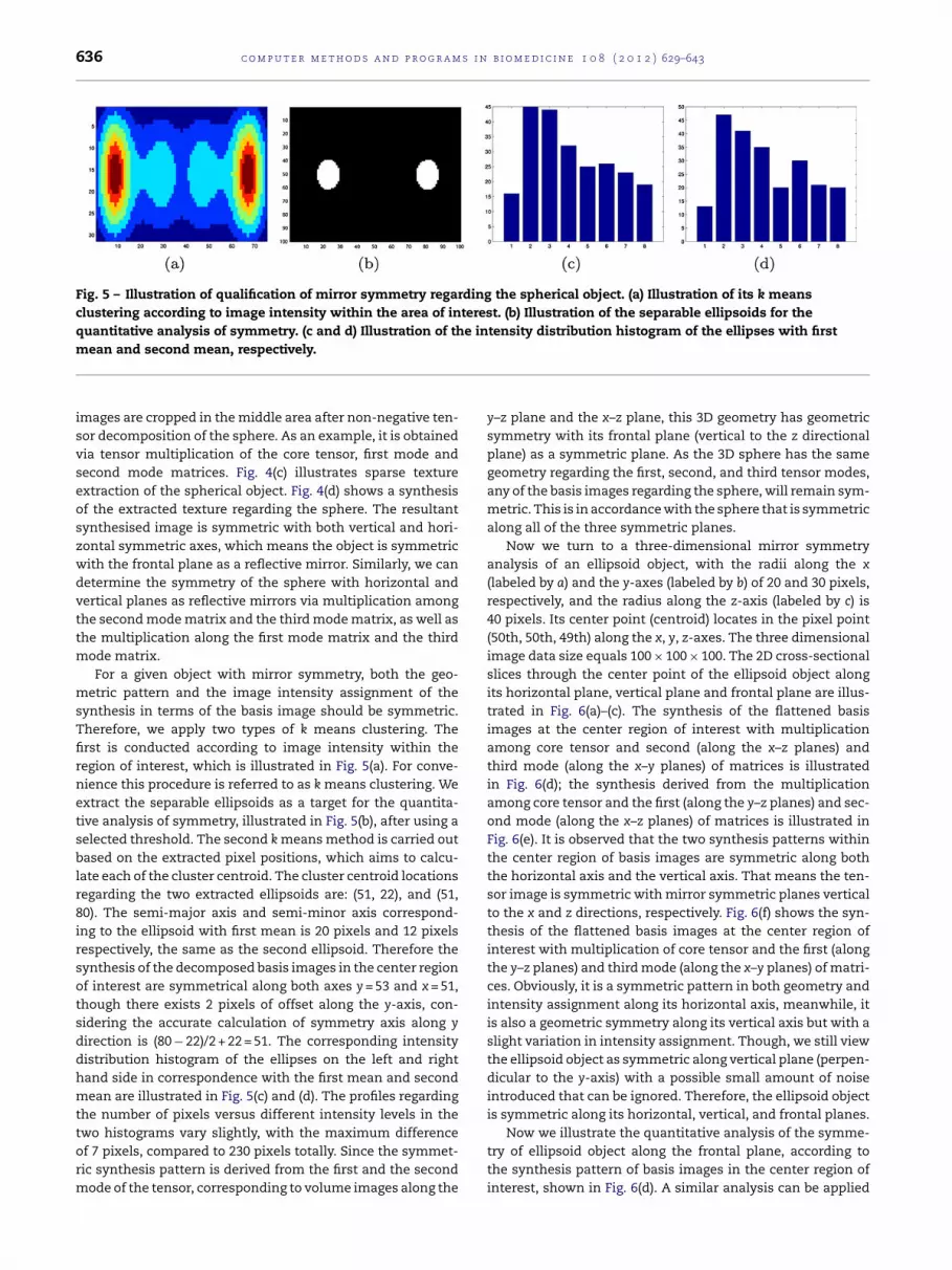
Fig. 5 – Illustration of qualification of mirror symmetry regarding the spherical object. (a) Illustration of its k meansclustering according to image intensity within the area of interest. (b) Illustration of the separable ellipsoids for thequantitative analysis of symmetry. (c and d) Illustration of the intensity distribution histogram of the ellipses with first

mean and second mean, respectively.

images are cropped in the middle area after non-negative ten-sor decomposition of the sphere. As an example, it is obtainedvia tensor multiplication of the core tensor, first mode andsecond mode matrices. Fig. 4(c) illustrates sparse textureextraction of the spherical object. Fig. 4(d) shows a synthesisof the extracted texture regarding the sphere. The resultantsynthesised image is symmetric with both vertical and hori-zontal symmetric axes, which means the object is symmetricwith the frontal plane as a reflective mirror. Similarly, we candetermine the symmetry of the sphere with horizontal andvertical planes as reflective mirrors via multiplication amongthe second mode matrix and the third mode matrix, as well asthe multiplication along the first mode matrix and the thirdmode matrix.

For a given object with mirror symmetry, both the geo-metric pattern and the image intensity assignment of thesynthesis in terms of the basis image should be symmetric.Therefore, we apply two types of k means clustering. Thefirst is conducted according to image intensity within theregion of interest, which is illustrated in Fig. 5(a). For conve-nience this procedure is referred to as k means clustering. Weextract the separable ellipsoids as a target for the quantita-tive analysis of symmetry, illustrated in Fig. 5(b), after using aselected threshold. The second k means method is carried outbased on the extracted pixel positions, which aims to calcu-late each of the cluster centroid. The cluster centroid locationsregarding the two extracted ellipsoids are: (51, 22), and (51,80). The semi-major axis and semi-minor axis correspond-ing to the ellipsoid with first mean is 20 pixels and 12 pixelsrespectively, the same as the second ellipsoid. Therefore thesynthesis of the decomposed basis images in the center regionof interest are symmetrical along both axes y = 53 and x = 51,though there exists 2 pixels of offset along the y-axis, con-sidering the accurate calculation of symmetry axis along ydirection is (80 − 22)/2 + 22 = 51. The corresponding intensitydistribution histogram of the ellipses on the left and righthand side in correspondence with the first mean and secondmean are illustrated in Fig. 5(c) and (d). The profiles regardingthe number of pixels versus different intensity levels in the

two histograms vary slightly, with the maximum differenceof 7 pixels, compared to 230 pixels totally. Since the symmet-ric synthesis pattern is derived from the first and the secondmode of the tensor, corresponding to volume images along the

y–z plane and the x–z plane, this 3D geometry has geometricsymmetry with its frontal plane (vertical to the z directionalplane) as a symmetric plane. As the 3D sphere has the samegeometry regarding the first, second, and third tensor modes,any of the basis images regarding the sphere, will remain sym-metric. This is in accordance with the sphere that is symmetricalong all of the three symmetric planes.

Now we turn to a three-dimensional mirror symmetryanalysis of an ellipsoid object, with the radii along the x(labeled by a) and the y-axes (labeled by b) of 20 and 30 pixels,respectively, and the radius along the z-axis (labeled by c) is40 pixels. Its center point (centroid) locates in the pixel point(50th, 50th, 49th) along the x, y, z-axes. The three dimensionalimage data size equals 100 × 100 × 100. The 2D cross-sectionalslices through the center point of the ellipsoid object alongits horizontal plane, vertical plane and frontal plane are illus-trated in Fig. 6(a)–(c). The synthesis of the flattened basisimages at the center region of interest with multiplicationamong core tensor and second (along the x–z planes) andthird mode (along the x–y planes) of matrices is illustratedin Fig. 6(d); the synthesis derived from the multiplicationamong core tensor and the first (along the y–z planes) and sec-ond mode (along the x–z planes) of matrices is illustrated inFig. 6(e). It is observed that the two synthesis patterns withinthe center region of basis images are symmetric along boththe horizontal axis and the vertical axis. That means the ten-sor image is symmetric with mirror symmetric planes verticalto the x and z directions, respectively. Fig. 6(f) shows the syn-thesis of the flattened basis images at the center region ofinterest with multiplication of core tensor and the first (alongthe y–z planes) and third mode (along the x–y planes) of matri-ces. Obviously, it is a symmetric pattern in both geometry andintensity assignment along its horizontal axis, meanwhile, itis also a geometric symmetry along its vertical axis but with aslight variation in intensity assignment. Though, we still viewthe ellipsoid object as symmetric along vertical plane (perpen-dicular to the y-axis) with a possible small amount of noiseintroduced that can be ignored. Therefore, the ellipsoid objectis symmetric along its horizontal, vertical, and frontal planes.

Now we illustrate the quantitative analysis of the symme-try of ellipsoid object along the frontal plane, according tothe synthesis pattern of basis images in the center region ofinterest, shown in Fig. 6(d). A similar analysis can be applied

c o m p u t e r m e t h o d s a n d p r o g r a m s i n b i o m e d i c i n e 1 0 8 ( 2 0 1 2 ) 629–643 637

Fig. 6 – Illustration of three-dimensional mirror symmetry analysis of an ellipsoid object. (a–c) Illustration of the 2Dcross-sectional slices through the center point of the ellipsoid object along its horizontal plane, vertical plane, and frontalplane. (d–f) The synthesis of the flattened basis images at the center region of interest with multiplication of core tensor andsecond and third mode matrices, of core tensor and the first and second mode matrices, and of core tensor and the first andthird mode matrices, respectively.

Fig. 7 – Illustration of quantification of mirror symmetry regarding the ellipsoid object. (a) Illustration of its k-meansclustering according to image intensity. (b) Illustration of the extracted separable synthesis patterns for quantitativeanalysis of symmetry. (c–f) Illustration of the intensity distribution histogram of the oval shape patterns counterclockwise.

638 c o m p u t e r m e t h o d s a n d p r o g r a m s i n b i o m e d i c i n e 1 0 8 ( 2 0 1 2 ) 629–643

Fig. 8 – Illustration of three-dimensional mirror symmetry analysis of object with lobules. (a) Illustration of one of the 2Dhorizontal plane cross-sectional slices, at the 40th pixel layer. (b and c) Illustration of one of the 2D cross-sectional slicesthrough the center point of the large ellipsoid object, along its vertical plane, and frontal plane. (d) Non-negative tensordecomposition of object with lobules. (e) Illustration of the synthesis of the extracted texture regarding the lobulation object.(f and g) Illustration of the two synthesis patterns derived from the part of the basis images with tensor multiplication of the

main

core tensor and the two mode matrices selected from the re

to qualify the symmetry along horizontal and vertical plane.The relevant k means clustering according to image intensityis shown in Fig. 7(a). The separable synthesis patterns areillustrated in Fig. 7(b), with cluster number larger than andequal to 5. The quantification of the symmetry of the 3Dellipsoid object is mainly focused on the analysis of the fourthreshold synthesis patterns illustrated in Fig. 7(b). It can beobserved that these threshold patterns allow to representthe symmetry of the whole synthesis pattern. The totalcentroid is located in the pixel position (51,51). The centroidpositions corresponding to the four threshold ellipses are:(38,64); (64,64); (38,37); (64,37). The four centroid positionsare symmetric along their vertical axis y = 51 and horizontalaxis x = 51. The distances between total centroid and thecentroid of each threshold pattern are: 18, 18, 19, 19, whichare symmetric along horizontal axis y = 51 and vertical axisx = 51, with slight offset of one pixel. The landmark positionsfrom four target patterns are: [(55,36),(72,36),(64,45),(63,31)];[(47,36),(30,36),(36,45),(35,31)]; [(47,66),(30,66),(34,71),(35,57)];[(72,66),(55,66),(62,71),(63,57)], which are approximately sym-metric along the x and y-axes with 1, and 2 pixel offsets,respectively. Combining these calculations, the extractedpatterns appear to be symmetric along vertical and hori-zontal axes. Fig. 7(c)–(f) illustrates the intensity distributionhistogram of the oval shape patterns counterclockwise. Eachhistogram is very similar, therefore, it is concluded that the3D ellipsoid object is symmetric along frontal plane.

One more experiment is to achieve three-dimensional mir-ror symmetry analysis of a 3D object with lobules. The spatial

geometry is designed with only symmetry along horizon-tal and frontal planes, which is to combine a large size ofellipsoid (a = 2/12 ; b = 3/12 ; c = 4/12) with a few small ellipsoidsarranged along its contours. Fig. 8(a) illustrates one of the

ing combinations.

2D cross-sectional slices along horizontal planes, at the 40thpixel layer. Fig. 8(b) and (c) illustrates one of the 2D cross-sectional slices through the center point of the large ellipsoidobject, along its vertical plane, and frontal plane, respectively.Fig. 8(d) illustrates non-negative tensor decomposition of theobject with lobulation. The basis images are obtained via mul-tiplication of core tensor, the third mode matrix and firstmode matrix. The flattened basis images are cropped in themiddle region. Fig. 8(e) shows the synthesis of the extractedtexture from the basis image. The resultant synthesis imagewith symmetry along both vertical and horizontal axes meansthe 3D image along the x–y plane and the y–z plane are sym-metric. So this pattern is symmetric with frontal plane as amirror, at least. Fig. 8(f) and (g) shows two synthesis patternsderived from cropped basis images with tensor multiplicationbetween the core tensor and the two mode matrices selectedfrom the remaining combinations. These two synthesis pat-terns are not symmetric along either of their symmetric axes,therefore, at least, the 3D object image is not symmetric alongthe x–z planes.

3.2. The second case

The second case is to explore the mirror symmetry of brainstructural MRI of white mass with rough resolution. The MRimage size is 47 ×58 × 43. Fig. 9(a)–(c) illustrates one of the 2Dcross-sectional slices along a horizontal plane, vertical plane,and frontal plane. Considering the 3D image is symmetric onthe x–y and the y–z planes, we change the modes of the MRI

datasets to a new MRI datasets, i.e. the third mode of originalMRI datasets becomes the first mode of the new matrix, thefirst and second become the second and the third in the newdatasets. Finally, we assemble the image datasets with size

c o m p u t e r m e t h o d s a n d p r o g r a m s i n b i o m e d i c i n e 1 0 8 ( 2 0 1 2 ) 629–643 639

Fig. 9 – Illustration of the mirror symmetry of brain structural MRI with rough resolution. The brain MRI size is 58 × 47 × 43.(a–c) Illustration of 2D cross-sectional slices along a horizontal plane, vertical plane, and frontal plane. (d) Illustration of ab

5uttwomltilltwwiip

atttbtg

cttfiFdptitpsatcw

rain slice image with asymmetry along an x–y plane.

8 ×47 ×43 into a tensor. We also rearrange the image vol-me structure to explore the asymmetry of the brain MRI viahe current algorithm. According to the generated datasets,he image volume with asymmetry is created as follows: first,e crop the part of images along the x–y plane, in order tobtain the images on the left hand side of the approximateirror structure of human brain. The extracted images at the

ayers from z = 7 to z = 22 are relocated to the layers with z = 5o z = 20 to create the first dataset with asymmetry, and themage datasets on the right hand side remain the same. Simi-arly, to increase the asymmetry, the extracted images on theeft hand side at the layers from z = 7 to z = 32 are relocatedo layers from z = 5 to z = 30, which form the second datasetith increased asymmetry. For comparison, the third datasetith further increased asymmetry is created by relocating the

mages from z = 7 to z = 42 to layers from z = 5 to z = 40. Fig. 9(d)llustrates the resultant image with asymmetry along the x–ylane.

The generated 3D images with symmetry and asymmetryre assembled into the third order tensors and non-negativeensor decomposition is applied to factorise the non-negativeensors to factors, with the core tensor size of 32 × 32 × 32 andhe basis image size of 58 × 1024. The center region of theasis images is cropped to a size of 58 ×180. Fig. 10(a)–(d) illus-rates the resultant synthesis for the symmetric MRI, and theenerated first, second, and third asymmetric MR images.

To ascertain the degree symmetry or the lack of it, k meanslustering is used to group the generated synthesis patternshat are normalised. Figs. 11(a), 12(a), 13(a) and 14(a) illustratehe resultant clustering in relation to symmetric brain MRI, therst, second and third asymmetric brain MRIs. As illustrated inig. 11(a), the part of the synthesis pattern marked by a whiteashed line is located in the center along which the synthesisattern is symmetric. Therefore it is viewed as a reference pat-ern. The positions of the reference pattern can also be foundn Fig. 12(a), 13(a) and 14(a), where they have been marked byhe white dashed lines. Shown in the mentioned figures, theatterns marked by white arrows on the left and right handide of the reference pattern, are two ellipses, which are useds the target patterns for the quantitative analysis of symme-

ry and asymmetry of the 3D brain MRIs. Quantitative analysisan be conducted based on the landmark points marked byhite solid lines. For clarification purposes, we illustrate the

zoomed version in Figs. 11(b), 12(b), 13(b), and 14(b). As men-tioned before, histogram images are used for the symmetryanalysis. Figs. 11(c) and (d), 12(c) and (d) 13(c) and (d) and 14(c)and (d) are histogram images of the synthesis patterns markedwith arrows shown in sub-figures labeled by (a) of the cor-responding figures, in terms of the four generated brain MRIdatasets. The four pairs of intensity histogram images showthat minor varieties happen among the right hand side of thesynthesis patterns, when the asymmetries are varied com-pared to the 3D symmetric brain MRI. For left hand side ofthe synthesis patterns, intensity levels are concentrated tothe first bin and first three bins when the asymmetry of 3Dimages varies from 25 layers to 35 layers, respectively. As aresult, there is a twofold rise in the number of pixels regard-ing the first and the first three bins, respectively, comparedbetween the left and the right hand side of the synthesis pat-terns. That means the asymmetry of intensity levels of thearrowed synthesis increases when the asymmetry of the 3Dimages increase.

For further quantitative analysis, we focus on the k meansclustering images with patterns marked by white arrows, forthe symmetric brain MRI and first, second, and third asym-metric brain MRI, referred to Figs. 11(a), 12(a), 13(a) and 14(a),respectively. We record the resultant calculations in Table 2.These are the centroid coordinates of each arrowed patternmarked by cross lines, and the coordinates of landmark pointsmarked by white solid lines in terms of the left and right handside of the clustering images with reference pattern markedby a white dashed line.

The axis of symmetry for each synthesis pattern remainsnearly the same, equal to x = 115 and y = 74. For the right syn-thesis patterns, the coordinates of the centroid are the samewith a value of [115,107], part of the pattern derived fromthe 3D images with 35 layer asymmetry, the coordinates ofthe centroid of which equal to [114,106], with one pixel offsetupward and towards the left, respectively. While regarding thecentroid positions on the-left-hand-side patterns, the x coor-dinates are moved down by 1,2,3 pixels with y coordinatesunchanged, corresponding to the symmetry, and the asym-

metry with 15 layers and 25 layers, respectively. The synthesispattern that comes from the 3D image with 35-layer asym-metry, shows a slight upward offset. For the four 3D imagedatasets with symmetry and increased asymmetry, we find

640 c o m p u t e r m e t h o d s a n d p r o g r a m s i n b i o m e d i c i n e 1 0 8 ( 2 0 1 2 ) 629–643

Fig. 10 – Illustration of the synthesised images related to the generated 3D brain structural MR image with symmetry (referto Fig. 9(a)–(c)) and asymmetry (refer to Fig. 9(a), (b), and (d)). (a–d) Illustration of the resultant synthesis for the symmetricbrain structural MRI, and the generated the first (with 15 asymmetric layers), the second (with 25 asymmetric layers), andthe third (with 35 asymmetric layers) asymmetric brain structural MR images, respectively.

Fig. 11 – Illustration of the synthesised pattern regarding a symmetric brain structural MRI with rough resolution. Thedimension that is assembled to a third order tensor equals to 58 × 47 × 43 pixels. (a) Illustration of the resultant k meansclustering. (b) Zoomed version of (a). (c and d) Illustration of intensity histogram images from the synthesis patterns marked

3.3. The third case

with white arrows.

that landmark points on the right-hand-side patterns are sym-metric according to their corresponding coordinates. However,on the left hand side of the arrowed synthesis patterns, x coor-dinates regarding the landmark points on the bottom moveaway from the symmetric positions of the top landmark pointsby 1, 4, 6, 3 pixels. The synthesis with 35-layer asymmetryshows slightly improved symmetry along the horizontal axis.

The distance of each pair of landmark points along vertical andhorizontal direction from left to right hand side, correspond-ing to the lengths of major and minor axis: [31:29; 18:18]; [32:28;

Fig. 12 – Illustration of the synthesis pattern regarding a brain st3D image. The asymmetric structure locates at the layers from z

clustering. (b) Zoomed version of (a). (c and d) Illustration of intenwith white arrows.

18:19]; [38:29; 18:18]; [39:25; 18:18]. The lengths of minor axesvary slightly and symmetrically, the lengths of major axes varyfrom 2, 4, 9–14. The asymmetry of the synthesis pattern alongthe vertical axis increases with the increase of asymmetry inthe 3D images.

For the structural brain MRIs of grey mass with high resolu-tion, we segment and crop the images in the middle regions

ructural MRI with 15 layers of asymmetric structure in its= 5 to z = 20. (a) Illustration of the resultant k meanssity histogram images from the synthesis patterns marked

c o m p u t e r m e t h o d s a n d p r o g r a m s i n b i o m e d i c i n e 1 0 8 ( 2 0 1 2 ) 629–643 641

Table 2 – The centroid coordinates and the coordinates of landmark points for each synthesis pattern with the signs ofarrows are depicted in Figs. 11(a), Fig. 12(a), 13(a) and 14(a).

Numberedlandmarkpoint

Coordinates

Symmetry 15 layer rearrangement 25 layer rearrangement 35 layer rearrangement

Left Right Left Right Left Right Left Right

Centroid [115,41] [115,107] [116,41] [115,107] [117,41] [115,107] [115,41] [114,106]1 [131,41] [130,107] [133,41] [129,107] [137,41] [129,107] [136,39] [127,107]2 [100,41] [101,107] [101,41] [101,107] [99,41] [100,107] [97,41] [102,107]

oivdstias

opoot

F3cw

F3cw

3 [115,50] [115,116] [115,50] [115,117]4 [115,32] [115,98] [115,32] [115,98]

f half of the symmetric brain along its x–y planes. Accord-ngly, we make a reflective symmetric image in 3D for goodisualisation of symmetry. Finally, we assemble the imageatasets with size 90 × 40 × 30 in to a tensor, which areymmetric along its horizontal and vertical planes. To createhe asymmetric structure for the 3D brain MRI, we extract halfmages on the left hand side at the layers from z = 15 to z = 26nd relocate them to the layers from z = 11 to z = 22, with theame size of tensor assembled for asymmetry analysis.

Fig. 15(a)–(c) illustrates one of the 2D cross-sectional slicesf structural brain MRI regarding grey mass along a horizontal

lane, vertical plane and frontal plane. Fig. 15(d)–(f) illustratesne of the 2D cross-sectional slices within the local regionf interest along a frontal plane, horizontal plane, and ver-ical plane. The cross-sectional slices along horizontal and

ig. 13 – Illustration of the synthesis pattern regarding a brain stD image. The asymmetric structure locates at the layers from z

lustering. (b) Zoomed version of (a). (c and d) Illustration of intenith white arrows.

ig. 14 – Illustration of the synthesis pattern regarding a brain stD image. The asymmetric structure locates at the layers from z

lustering. (b) Zoomed version of (a). (c and d) Illustration of intenith white arrows.

[114,50] [115,116] [115,49] [115,116][114,32] [115,98] [115,33] [115,98]

vertical planes are fully reflective symmetric. Fig. 15(g) is theimage with asymmetry along its horizontal plane. The synthe-sis patterns regarding the 3D MRI with generated symmetricand asymmetric structures are illustrated in Fig. 16(a) and(b), which are derived from the tensor multiplication of thedecomposed core tensor and the first and second mode ofmatrices. Fig. 16(a) shows an approximately symmetric struc-ture due to the symmetry properties along both horizontaland vertical planes of the tensor images. Fig. 16(b) shows anobvious elimination of symmetry when the symmetric struc-ture of the corresponding tensor images is diminished. The

resultant symmetry and asymmetry are in accordance with3D images with generated symmetric and asymmetric struc-ture along their horizontal and vertical planes. Fig. 16(a) and(b) is the zoomed in version of (c) and (d) for clear comparison.

ructural MRI with 25 layers of asymmetric structure in its= 5 to z = 30. (a) Illustration of the resultant k meanssity histogram images from the synthesis patterns marked

ructural MRI with 35 layers of asymmetric structure in its= 5 to z = 40. (a) Illustration of the resultant k means

sity histogram image from the synthesis patterns marked

642 c o m p u t e r m e t h o d s a n d p r o g r a m s i n b i o m e d i c i n e 1 0 8 ( 2 0 1 2 ) 629–643

Fig. 15 – (a–c) Illustration of one of the 2D cross-sectional slices of structural brain MRI with high resolution showing greymass along a horizontal plane, vertical plane and frontal plane, respectively. The brain structural MRI with a size of90 × 40 × 30 are assembled to a 3rd order tensor. (d–g) Illustration of one of the 2D cross-sectional slices regarding croppedMRI datasets of grey mass along a frontal plane, horizontal plane, and vertical plane, respectively. (g) Illustration of one ofthe cross-sectional images with asymmetry along its horizontal plane.

Fig. 16 – (a and b)Illustration of the synthesised patterns regarding the 3D brain structural MRIs with generated symmetric(the size of 90 × 40 × 30) and asymmetric structures inserted into the layers between z = 11 and z = 22, respectively. (c and d)

Zoomed version of (a) and (b).

Illustrated in Fig. 16, the position in the center region is markedby the white dashed line, which is viewed as a symmetry axis.

4. Conclusion

A sparse decomposition scheme for the detection of sym-metric structures in 3-dimensional spaces is presented. Theapproach is based on the decomposed basis images via non-negative tensor factorisation to look at the symmetry of spatialshapes. It is shown that the reflectional symmetries can bequantified by the synthesis pattern of directional textures,which is an effective expansion of sparse basis elements.We apply this approach to the analysis of image geometry

in 3D with aims for the discrimination of symmetry andasymmetry, as well as estimating the different degree of asym-metry. The datasets involved are related to spatial geometricshapes with simulation of different types of tumors (spherical,

ellipsoid, lobuled). The resulting scheme is shown experimen-tally to be both effective and is able to detect symmetricstructures embedded in real images.

Future work will consider extensions of the application ofthe proposed methods on MRI detection of breast cancer, andbrain-disease detection using brain structural MRIs. Regard-ing breast cancer detection via MRIs, it will be desirable toapply proper segmentation algorithms to define tumor regionsfor shape analysis. This work can also be extended to greyand color images in 3D for quantitative analysis of symmetricstructure.

Conflict of interest

None declared.

i n b i

r

c o m p u t e r m e t h o d s a n d p r o g r a m s

e f e r e n c e s

[1] M. Kazhdan, B. Chazelle, D. Dobkin, T. Funkhouser, S.Rusinkiewicz, A reflective symmetry descriptor for 3Dmodels, Algorithmica 38 (1) (2004) 201–225.

[2] T. Sawada, Visual detection of symmetry of 3D shapes,Journal of Vision 10 (6) (2010) 1–22.

[3] D. Shen, H. Ip, K. Cheung, E. Teoh, Symmetry detection bygeneralized complex (GC) moments: a close-form solution,IEEE Transactions on Pattern Analysis and MachineIntelligence 21 (5) (1999) 466–476.

[4] C. Sun, D. Si, Fast reflectional symmetry detection usingorientation histograms, Real-Time Imaging 5 (1) (1999) 63–74.

[5] C. Sun, J. Sherrah, 3-D symmetry detection using theextended Gaussian image, IEEE Transactions on PatternAnalysis and Machine Intelligence 19 (2) (1997) 164–165.

[6] G. Marola, On the detection of the axes of symmetry ofsymmetric and almost symmetric planar images, IEEETransactions on Pattern Analysis and Machine Intelligence11 (1) (1989) 104–108.

[7] D.E. Knuth, J.H. Morris, V.R. Pratt, Fast pattern matching instrings, SIAM Journal on Computing 6 (2) (1977) 323–350.

[8] D. O’Mara, R. Owens, Measuring bilateral symmetry indigital images, in: 1996 IEEE Region 10 Conference on DigitalSignal Processing Applications (TENCON 96), vols. 1 and 2,1996, pp. 151–156.

[9] S. Derrode, F. Ghorbel, Shape analysis and symmetrydetection in gray-level objects using the analyticalFourier–Mellin representation, Signal Processing 84 (1) (2004)25–39.

[10] L. Lucchese, Frequency domain classification of cyclic anddihedral symmetries of finite 2D patterns, PatternRecognition 37 (12) (2004) 2263–2280.

[11] Y. Keller, Y. Shkolnisky, A signal processing approach tosymmetry detection, IEEE Transaction on Image Processing15 (6) (2006) 2198–2207.

[12] D. Reisfeld, H. Wolfson, Y. Yeshurun, Context freeattentional operators: The generalized symmetry transform,International Journal of Computer Vision 14 (2) (1995)119–130.

[13] M. Chertok, Y. Keller, Spectral symmetry analysis, IEEETransactions on Pattern Analysis and Machine Intelligence32 (7) (2010) 1227–1238.

[14] W. Yang, S. Zhang, Y. Chen, W. Li, Y. Chen, Shape symmetryanalysis of breast tumors on ultrasound images, Computersin Biology and Medicine 39 (3) (2009) 231–238.

[15] M. Herbert, D. Ziegler, C. Deutsch, L. O’Brien, D. Kennedy, P.Filipek, A. Bakardjiev, J. Hodgson, M. Takeoka, N. Makris, V.Caviness, Brain asymmetries in autism and developmentallanguage disorder: a nested whole-brain analysis, Brain 128(1) (2005) 213–226.

[16] R. Alterson, D.B. Plewes, Bilateral symmetry analysis ofbreast MRI, Physics in Medicine and Biology 48 (20) (2003)3431–3443.

[17] Y. Sun, B. Bhanu, S. Bhanu, Automatic symmetry-integratedbrain injury detection in MRI sequences, in: IEEE ComputerSociety Conference on Computer Vision and Pattern

Recognition Workshops, 2009, 2009, pp. 79–86.

[18] M.P. Friedlandera, K. Hatzb, Computing non-negative tensorfactorizations, Optimization Methods & Software 23 (4)(2008) 631–647.

o m e d i c i n e 1 0 8 ( 2 0 1 2 ) 629–643 643

[19] G. Peyré, Sparse modeling of textures, Journal ofMathematical Imaging and Vision 34 (1) (2009) 17–31.

[20] VAMCA, Vamca: Cortical Meta-Analysis Toolbox,http://www.nitrc.org/projects/vamca/, 2010.

[21] BrainWeb, Brainweb: Simulated Brain Database,http://www.nitrc.org/projects/vamca/, 2010.

[22] J. Mairal, F. Bach, J. Ponce, G. Sapiro, Online learning formatrix factorization and sparse coding, Journal of MachineLearning Research 11 (2010) 19–60.

[23] M.D. Plumbley, S.A. Abdallah, J.P. Bello, M.E. Davies, G. Monti,M.B. Sandler, Automatic music transcription and audiosource separation, Cybernetics and Systems 33 (6) (2002)603–627.

[24] K.I. Kim, K. Jung, H.J. Kim, Face recognition using kernelprincipal component analysis, IEEE Signal Processing Letters9 (2) (2002) 40–42.

[25] M.S. Bartlett, J.R. Movellan, T.J. Sejnowski, Face recognitionby independent component analysis, IEEE Transactions onNeural Networks 13 (6) (2002) 1450–1464.

[26] G. Peyré, Texture synthesis with grouplets, IEEE Transactionson Pattern Analysis and Machine Intelligence 32 (4) (2010)733–746.

[27] H. Lee, Y. Kim, A. Cichocki, S. Choi, Nonnegative tensorfactorization for continuous EEG classification, InternationalJournal of Neural Systems 17 (4) (2007) 305–317.

[28] A. Cichocki, R. Zdunek, A.H. Phan, S. Amari, NonnegativeMatrix and Tensor Factorizations Applications toExploratory Multi-way Data Analysis and Blind SourceSeparation, John Wiley & Sons, Inc., Chichester, UK, 2009.

[29] M. Vasilescu, D. Terzopoulos, Multilinear subspace analysisof image ensembles, in: 2003 IEEE Computer SocietyConference on Computer Vision and Pattern Recognition,vol. II, 2003, pp. 93–99.

[30] T. Hazan, S. Polak, A. Shashua, Sparse image coding using a3D non-negative tensor factorization, 10th IEEEInternational Conference on Computer Vision (ICCV 2005),vols. 1 and 2 (2005) 50–57.

[31] L. Tucker, Some mathematical notes on three-mode factoranalysis, Psychometrika 31 (3) (1966) 279–311.

[32] B. Bader, T. Kolda, Efficient MATLAB computations withsparse and factored tensors, SIAM Journal on ScientificComputing 30 (1) (2008) 205–231.

[33] S. Aja-Fernández, R. de Luis Garcia, D. Tao, X. Li, Tensors inImage Processing and Computer Vision (Advances in PatternRecognition), Springer-Verlag, New York, USA, 2009.

[34] T. Zhang, G. Golub, Rank-one approximation to high ordertensors, Matrix Analysis and Applications 23 (2) (2001)534–550.

[35] A. Conn, N. Gould, P. Toint, Trust-region methods, MPS-SIAMSeries on Optimization, Society of Industrial and AppliedMathematics, Philadelphia, 2000.

[36] C. Paige, M. Saunders, LSQR: an algorithm for sparse linearequations and sparse least squares, ACM Transaction onMathematical Software 8 (1) (1982) 43–71.

[37] Elad, Sparse & redundant representation modeling ofimages: theory and applications, Seventh InternationalConference on Curves and Surfaces 39 (3) (2010) 231–238.

[38] M. Elad, M. Aharon, Image denoising via sparse andredundant representations over learned dictionaries, IEEE

Transactions on Image Processing 15 (12) (2006) 3736–3745.

[39] B.A. Olshausen, D.J. Field, Emergence of simple-cellreceptive field properties by learning a sparse code fornatural images, Nature 381 (13) (1996) 607–609.