Seediscussions,stats,andauthorprofilesforthispublicationat:https://www.researchgate.net/publication/225977423

Testingthetailindexinautoregressivemodels

ARTICLEinANNALSOFTHEINSTITUTEOFSTATISTICALMATHEMATICS·SEPTEMBER2009

ImpactFactor:0.82·DOI:10.1007/s10463-007-0155-z

CITATIONS

5

READS

16

3AUTHORS,INCLUDING:

JanaJureckova

CharlesUniversityinPrague

140PUBLICATIONS1,917CITATIONS

SEEPROFILE

JanPicek

TechnicalUniversityofLiberec

54PUBLICATIONS442CITATIONS

SEEPROFILE

Availablefrom:JanPicek

Retrievedon:04February2016

Ann Inst Stat Math (2009) 61:579–598DOI 10.1007/s10463-007-0155-z

Testing the tail index in autoregressive models

Jana Jurecková · Hira L. Koul · Jan Picek

Received: 8 May 2006 / Revised: 21 June 2007 / Published online: 14 September 2007© The Institute of Statistical Mathematics, Tokyo 2007

Abstract We propose a class of nonparametric tests on the Pareto tail index of theinnovation distribution in the linear autoregressive model. The simulation study illus-trates a good performance of the tests. Such tests have various applications in a study offlood flows, rainflow data, behavior of solids, atmospheric ozone layer and reliabilityanalysis, in communication engineering, in stock markets and insurance.

Keywords Empirical process · Heavy tailed distribution · Feigin-Resnick estimator ·Pareto tail index

1 Introduction

If we are interested in the extremal events such as the extreme intensity of the wind,the high flood levels of the rivers or extreme values of environmental indicators, then

Research of J. Jurecková and J. Picek was partly supported by Czech Republic Grant 201/05/2340, by theResearch Project LC06024 and by the NSF grant DMS 0071619. Research of H. L. Koul was partlysupported by the NSF grants DMS 0071619 and 0704130.

J. Jurecková (B)Department of Probability and Mathematical Statistics, Charles University in Prague, Sokolovská 83,186 75 Prague 8, Czech Republice-mail: jurecko@karlin.mff.cuni.cz

H. L. KoulDepartment of Statistics and Probability, Michigan State University, A413 Wells Hall, East Lansing,MI 48824-1027, USAe-mail: koul@stt.msu.edu

J. PicekDepartment of Applied Mathematics, Technical University in Liberec, Hálkova 6, 461 17 Liberec 1,Czech Republice-mail: jan.picek@tul.cz

123

580 J. Jurecková et al.

we are rather interested in the tails of the underlying distribution than in its centralpart. A goodness-of-fit test does not provide us with a sufficient information on theshape of tails, because it concerns mostly the central part. It is important to decidewhether the probability distribution function is light- or heavy-tailed. If we decide infavor of a heavy tail, in the next step we should study more closely the shape of thetail, and make the pertinent decisions.

Testing the hypothesis on the tail index of a heavy tailed distribution is an alterna-tive inference to the classical point estimation, surprisingly not yet much elaboratedin the literature, though the tests often work under weaker conditions than the pointestimators, can be easily reconverted into the confidence sets, and have an intuitiveinterpretation.

In the present paper, we construct a class of tests on the tail index of the innovationdistribution in the linear autoregressive model. Such tests have applications in theenvironmental and financial time series, among others.

Consider the AR(p) model where the observation Xt satisfies

Xt = ρ1 Xt−1 + · · · + ρp Xt−p + εt , t = 0,±1,±2, . . . , (1)

where ρ := (ρ1, . . . , ρp)′ ∈ R

p is an unknown parameter and εt , t = 0,±1,±2, . . . ,are independent identically distributed (i.i.d.) random variables with a heavy-taileddistribution function F satisfying

limx→∞

− ln(1 − F(x))

m ln x= 1 (2)

for some m > 0. The l’Hospital rule and the von Mises condition (see Embrechts etal. (1997), Chap. 3, Theorem 3.3.7) imply that the distributions of type (2) satisfy

1 − F(x) = x−m L(x), x ≥ x0, (3)

for some x0 > 0, where L stands for a positive function, slowly varying at infinity.In the sequel, L , with or without a suffix will stand for such a function. Moreover,we shall throughout assume that the d.f. F is absolutely continuous having Lebesguedensity f .

We shall assume that the time series is strictly stationary. According to Proposition13.3.2 in Brockwell and Davis (1991, p. 537), a sufficient condition for this is that1 − ρ1z − · · · − ρpz p �= 0 for |z| ≤ 1. Moreover, then

Xt =∞∑

t=0

ψ jεt− j , a.s., (4)

with ψ ′j s such that

∑∞t=0 |ψ j |γ < ∞, for 0 < γ < 1

m ∧ 1. On the other hand, fromTheorem 3.3.7 of Embrechts et al. (1997), we obtain that under (3), for any finite n,

max1≤t≤nN

|εt | = Op(N1m L1(N )), as N → ∞.

123

Testing the tail index in autoregressive models 581

This and (4) in turn imply

max1≤t≤nN

|Xt | = Op(N1m L1(N )), max

1≤t≤nN‖Yt‖ = Op(N

1m L1(N )), (5)

where Yt−1 := (Xt−1, . . . , Xt−p)′, t = 0,±1, . . . .

Let m0 > 0 be a fixed number. The problem of interest is to test either of thefollowing two hypotheses:

H0 : F is of type (3), concentrated on the positive half-axis, satisfying

xm0(1 − F(x)) ≥ 1, for x > x0,

with hypothetical 0 < m0 ≤ 2 and for some x0 ≥ 0,

against the alternative

K0 : F is of type (3), concentrated on the positive half-axis, and limx→∞xm0

(1 − F(x)) < 1,or

H1 : F is of type (3) satisfying

xm0(1−F(x))≥1, for x> x0, with hypothetical m0 > 2, for some x0 ≥ 0,

against the alternativeK1 : F is of type (3) satisfying limx→∞xm0(1 − F(x)) < 1, with m0 > 2.

In either of these cases we wish to test the hypothesis that the right tail of F isthe same or heavier than that of the Pareto distribution with index m0 against thealternative that the right tail of F is lighter. The reason for distinguishing between H0and H1 is that one needs to use different estimators of autoregressive parameters inthese two cases, which in turn impose different conditions on the model.

Due to (3), the problem of identifying the tails is semiparametric in its nature,involving a nuisance slowly varying function, hence the hypothesis H1 is the set ofall distribution functions either of the form 1 − F(x) = x−m0 L(x) where L(x) runsover all slowly varying functions such that L(x) ≥ 1 for x > x0, or of the form1 − F(x) = x−m L(x) with m < m0 and with a positive slowly varying function L .H0 is an analogous set of distributions concentrated on the positive half-axis.

Numerous authors have considered the problem of testing the Gumbel hypothesis,Hg : m = ∞ against m < ∞ : we refer to Castillo et al. (1989), Galambos (1982),Gomes (1989), Gomes and Alpuim (1986), Hasofer and Wang (1992), Hosking (1984),van Montfort and Gomes (1985), van Montfort and Witter (1985), Stephens (1977),Tiago de Oliveira (1984). Others, as Falk (1995a,b), Marohn (1994, 1998a,b), studiedtesting the Gumbel hypothesis in the frame of the local asymptotic normality (LAN).Such tests, when they reject the Gumbel hypothesis in favor of alternative m < ∞,

do not provide any information on the heaviness of the tail of the distribution, whilejust that is just the information needed in practical applications.

123

582 J. Jurecková et al.

The proposed tests of H0 and H1 are based on the extremes of segments of theresidual empirical process. Tests on the Pareto index for the i.i.d. model were con-structed by Fialová et al. (2004), Jurecková, and Picek (2001) and by Picek andJurecková (2001). Tests on the tail index of errors in the linear regression model, basedon the extreme regression quantiles, were proposed by Jurecková (1999). However,tests based on the residuals seem to be preferable, and we expect a similar phenomenonto hold in the linear AR time series.

Because the proposed tests are based on the residual empirical process of the ARseries, in the next section we first analyze the asymptotic behavior of such processes.The tests and their asymptotic null (normal) distributions are given in Sect. 3, whileSect. 4 deals with their consistency. Section 5 is a numerical illustration.

2 Residual empirical process

Let n, N be positive integers and let ρN be an estimator of ρ in (1) based on the dataset X1−p, X2−p, . . . , X0, X1, . . . , XnN ; the estimators will be considered later.

Letεt := Xt − ρ′

N Yt−1, t = 1 − p, 2 − p, . . . , nN , (6)

with Yt−1 given in (5).Now group these residuals in N groups, each of size n, so that the residuals in the

t th group are ε(t−1)n−p+1, . . . , εtn−p. Do a similar decomposition of the errors {εt }.Let

εt(n) := max

1≤i≤nε(t−1)n−p+i , εt

(n) := max1≤i≤n

ε(t−1)n−p+i , t = 1, 2, . . . , N . (7)

The empirical distribution function F∗N of the maximal errors {εt

(n), t = 1, . . . , N }is approximated by the empirical distribution function F∗

N of the maximal residuals{εt(n), t = 1, . . . , N }, where

F∗N (x) := N−1

N∑

t=1

I [εt(n) ≤ x], F∗

N (x) := N−1N∑

t=1

I [εt(n) ≤ x], x ∈ R. (8)

Puta(1)N ,m := (nN 1−δ)1/m, 0 < δ < 1 (9)

or alternatively

a(2)N ,m :=(

nN (ln N )−2+η)1/m, 0 < η < 1. (10)

The effect of the choice of parameters δ and η is discussed in Sect. 5.We shall first show that

|F∗N (aN ,m)− F∗

N (aN ,m)| = op(1) as N → ∞ and for a fixed n, (11)

123

Testing the tail index in autoregressive models 583

under (3) and with an appropriate estimate ρN of ρ in (6), provided m is the true valueof the tail index.

To prove (11), we need to find an estimate ρN such that, for some sequence ofpositive numbers dN → ∞,

dN (ρN − ρ) = Op(1). (12)

Possible choices of the estimator are discussed in Sect. 2.1.If (12) is true, we can write

εt = εt − (ρN − ρ)′Yt−1 = εt − d−1N dN (ρN − ρ)′Yt−1.

In view of (5) and (12), for any κ > 0, there is a C < ∞ and an Nκ < ∞, such thatfor all N > Nκ ,

P(‖dN (ρN − ρ)‖ ≤ C

) ≥ 1 − κ, P

(max

1≤t≤nN‖Yt‖ ≤ C N 1/m L1(N )

)≥ 1 − κ.

(13)For ∀ u ∈ R

p, let

F∗N (a

(ν)N ,m,u) = N−1

N∑

t=1

n∏

i=1

I[ε(t−1)n−p+i ≤ a(ν)N ,m + d−1

N u′Y(t−1)n−p+i

], (14)

ν = 1, 2, and consider the behavior of the sequences

D(ν)N := sup

‖u‖≤C

∣∣∣F∗N (a

(ν)N ,m,u)− F∗

N (a(ν)N ,m)

∣∣∣ , ν = 1, 2. (15)

For any d.f. G on R, let G−1(u) := inf{x : G(x) ≥ u}, 0 ≤ u ≤ 1. Let

ξN := F−1 (1 − 1

N

) = N 1/m L1(N ) (16)

be the “population extreme” of F , and let

∆(ν)N := F

(a(ν)N ,m + d−1

N C2 ξN

)− F

(a(ν)N ,m − d−1

N C2 ξN

), ν = 1, 2,

(17)AN :=

{max

1≤t≤nN‖Yt‖ ≤ C ξN

},

with C as in (13). Moreover, let UNi (x) := FNi (x) − F(x), i = 1, . . . , n, whereFNi (x) is the empirical d.f. of {ε(t−1)n−p+i , 1 ≤ t ≤ N }, i = 1, . . . , n. Using thefact that indicators are monotonic functions of their arguments and bounded by 1, andthe identity

M∏

i=1

ai −M∏

i=1

bi =M∑

i=1

[ai − bi ]i−1∏

k=1

ak

M∏

k=i+1

bk,

123

584 J. Jurecková et al.

that is valid for any positive integer M and for any real numbers {ai , bi }Mi=1, we obtain

that an upper bound for D(ν)N on the set AN ,

D(ν)N ≤ N−1

N∑

t=1

n∑

i=1

I[a(ν)N ,m − d−1

N C2 ξN ≤ ε(t−1)n−p+i ≤ a(ν)N ,m + d−1N C2 ξN

]

=n∑

i=1

[UNi (a

(ν)N ,m + d−1

N C2 ξN )− UNi (a(ν)N ,m − d−1

N C2 ξN )]

+ n∆(ν)N

= D(ν)N1 + n∆(ν)N (say), ν = 1, 2. (18)

Using the embedding theorem of Komlós et al. (1975) for empirical process UNi (x),we find that there are sequences of independent Brownian bridges BNi , i = 1, . . . , n,N = 1, 2, . . . , such that

D(ν)N1 = N−1/2

n∑

i=1

[BNi (F(a

(ν)N ,m + d−1

N C2 ξN ))− BNi (F(a(ν)N ,m − d−1

N C2 ξN ))]

+O(N−1 ln N ), a.s., ν = 1, 2 (19)

and the differences of the Brownian bridges in (19) are of the orders(∆(ν)N

)1/2,

ν = 1, 2. On the other hand, from (3), (9) and (10) follow approximations for densityf of F :

f (a(1)N ,m) ≈ m(nN )−(1−δ)

(1+ 1

m

)

L(N )(20)

f (a(2)N ,m) ≈ m(nN )−

(1+ 1

m

)

(ln N )

(1+ 1

m

)(2−η)

L(N )

where aN ,m ≈ bN means that aN ,m/bN → 1 as N → ∞. Hence, (16) and (17) implythat

∆(1)N ≈ C2 K m d−1

N ξN f (a(1)N ,m) ≈ C2 K m N−

(1−δ m+1

m

)

L(N ) d−1N ,

(21)∆(2)N ≈ C2 K m d−1

N ξN f (a(2)N ,m) ≈ C2 K m N−1(ln N )m+1

m (2−η)L(N ) d−1N

and, regarding (6), we obtain

D(1)N1 = Op

(N

−1+ δ2

(1+ 1

m

)

L12 (N ) d

− 12

N

),

(22)D(2)

N1 = Op

(N−1(ln N )(1− η

2 )(1+ 1m )L

12 (N ) d

− 12

N

).

123

Testing the tail index in autoregressive models 585

Finally, (15), (18), (21) and (22) together would lead to the orders for D(ν)N :

D(1)N = Op

(N

−1− δ2

(1+ 1

m

)

L12 (N ) d

− 12

N

)+ O

(N

−1+δ(

1+ 1m

)

L(N ) d−1N

),

D(2)N = Op

(N−1(ln N )(

1− η2 )

(1+ 1

m

)

L12 (N ) d

− 12

N

)(23)

+ O

(N−1(ln N )

(2−η)(

1+ 1m

)

L(N ) d−1N

).

In the next subsection, we shall consider more closely the possible choice of estima-tor ρN and the associated choice of dN in (12), in order to find the rate of convergencein (11).

2.1 Estimators of autoregression coefficients

The choice of estimator ρN heavily depends on our hypothetical value m0 of the tailindex. Generally, we should distinguish two cases for the hypothetical distribution ofinnovations:

(i) Heavy-tailed distribution satisfying (3) with 0 < m0 ≤ 2;(ii) distribution satisfying (3) with m0 > 2.

ad (i): For distributions of the first group we find the linear programming estimatorof ρ, proposed by Feigin and Resnick (1994), as the most convenient.It is defined as

ρL P := argmaxu∈DN

p∑

j=1

u j ,

(24)

DN :=⎧⎨

⎩u ∈ Rp : Xt ≥

p∑

j=1

u j Xt− j , t = 1, . . . , nN

⎫⎬

⎭ .

Feigin and Resnick considered a stationary autoregressive process with positive inno-vations, whose distribution satisfies the conditions

p∑

j=1

ρ j < ∞, (25)

lims→∞

1 − F(sx)

1 − F(s)= x−α, for all x > 0 and for some α > 0, (26)

IE(ε−βt ) =∫ ∞

0u−βdF(u) < ∞, for someβ > α. (27)

Distributions of type (3) satisfy (26) with α = m. As examples of distributionssatisfying condition (27), Feigin and Resnick mention positive stable densities; (27)

123

586 J. Jurecková et al.

is satisfied, e.g. by the inverse normal distribution, the Fréchet distribution and thePareto distribution with

1 − F(x) ={

x−m for x > 11 otherwise.

Under these conditions, Feigin and Resnick proved that ρL P satisfies (12) with

dN := F−1(

1 − 1

nN

)= (nN )

1m L(N ) = O(N

1m L(N )). (28)

If the autoregressive process satisfies the Feigin and Resnick conditions and the resi-duals in (6) are calculated with respect to ρL P , then the bounds in (22) are of therespective orders

D(1)N = Op

(N−1+ δ

2 − 1−δ2m L1/2(N )

)+ O

(N−1+δ− 1−δ

m L(N )),

D(2)N = Op

(N

−(

1+ 12m

)

(ln N )(1− η

2 )(

1+ 1m

)

L1/2(N )

)

+ O

(N

−(

1+ 1m

)

(ln N )(2−η)

(1+ 1

m

)

L(N )

).

Hence, as N → ∞,

N 1− δ2 D(1)

N = op(1), ∀ δ < 2/(m + 2),(29)

N (ln N )−1+ η2 D(2)

N = op(1).

ad (ii): If F belongs to the second group, then we need not to restrict ourselvesto positive innovations. The most convenient estimators of ρ for distributions withm0 > 2 are either GM-estimators or GR-estimators; we refer to Koul (2002) for theirdescription and profound study. These estimators are

√N -consistent, and cover the

popular Huber estimator; the distribution can be extended over all real line and (11)applies for ν = 1, 2.

3 Construction of the tests

Our procedures are based on the dataset of observations X1−p, X2−p, . . . , X0,

X1, . . . XnN . If we want to test H0 with 0 < m0 ≤ 2, then we calculate the resid-uals with respect to the linear programming estimator ρL P , defined in (24). If wewant to test H1 with m0 > 2, then we calculate the residuals with respect to GM- orGR-estimators (see Koul 2002). Let a(1)N ,m0

, a(2)N ,m0be as in (9), (10), respectively;

calculate F∗N (a

(ν)N ,m0

), ν = 1, 2, as per the definition (8).We propose two tests for both H0 against K0 and H1 against K1, respectively,

corresponding to a(1)N ,m0, a(2)N ,m0

, respectively. The first test is based on the same

123

Testing the tail index in autoregressive models 587

threshold a(1)N ,m0as the test for i.i.d. observations proposed by Jurecková, and Picek

(2001). The higher value a(2)N ,m0in the second test is likely to reduce the probability of

error of the first kind, though it leads to a slower convergence to the asymptotic nulldistribution.Test (1): The test of H0 against K0 and of H1 against K1, respectively, rejects thehypothesis provided

either 1 − F∗N (a

(1)N ,m0

) = 0,

or 1 − F∗N (a

(1)N ,m0

) > 0 (30)

and N δ/2[− ln(1 − F∗

N (a(1)N ,m0

))− (1 − δ) ln N]

≥ Φ−1(1 − α),

where Φ is the standard normal distribution function and α ∈ (0, 1) is the asymptoticsignificance level.Test (2): The test of H0 against K0 and of H1 against K1, respectively, rejects thehypothesis provided

either 1 − F∗N (a

(2)N ,m0

) = 0,

or 1 − F∗N (a

(2)N ,m0

) > 0, and (31)

(ln N )1− η2

[− ln(1 − F∗

N (a(2)N ,m0

))− ln N + (2 − η) ln ln N]

≥ Φ−1(1 − α).

The following theorems show that the test criteria (30) and (31) have asymptoticallystandard normal distributions under the exact Pareto tail corresponding to 1− F(x) =x−m0 , for x > x0.

Theorem 3.1 Consider the stationary autoregressive process (1).(I) Assume that the process (1) satisfies the condition (25) and that the innovation dis-tribution function F is absolutely continuous and of type (3) with tail index m0, 0 <m0 ≤ 2, concentrated on the positive half-axis and strictly increasing on the set{x : F(x) > 0}. Let F∗

N (a(1)N ,m0

) be the empirical distribution function of extremeresiduals of N segments of length n, defined in (8), where the residuals are calculatedwith respect to ρL P defined in (24). Then, the following hold.

(i) For every distribution P satisfying H0,

limN→∞ P

(0 < F∗

N (a(1)N ,m0

) < 1)

= 1. (32)

(ii) If 1 − F(x) = x−m0 , ∀ x > x0, then

limN→∞ P

{N δ/2

[−ln(1− F∗

N (a(1)N ,m0

))−(1 − δ) ln N]

≤ x}

= Φ(x), ∀ x ∈ R.

(33)

123

588 J. Jurecková et al.

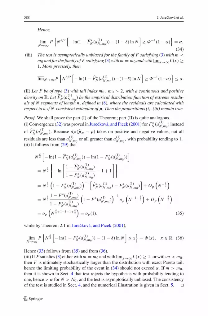
Hence,

limN→∞ P

{N δ/2

[− ln(1 − F∗

N (a(1)N ,m0

))− (1 − δ) ln N]

≥ Φ−1(1 − α)}

= α.

(34)(iii) The test is asymptotically unbiased for the family of F satisfying (3) with m <

m0 and for the family of F satisfying (3) with m = m0 and with limx→∞L(x) ≥1. More precisely, then

limN→∞ P{

N δ/2[− ln(1 − F∗

N (a(1)N ,m0

))−(1−δ) ln N]

≥ Φ−1(1−α)}

≤ α.

(II) Let F be of type (3) with tail index m0, m0 > 2, with a continuous and positivedensity on R. Let F∗

N (a(1)N ,m0

) be the empirical distribution function of extreme residu-als of N segments of length n, defined in (8), where the residuals are calculated withrespect to a

√N-consistent estimator of ρ. Then the propositions (i)–(iii) remain true.

Proof We shall prove the part (I) of the Theorem; part (II) is quite analogous.(i) Convergence (32) was proved in Jurecková, and Picek (2001) for F∗

N (a(1)N ,m0

) instead

of F∗N (a

(1)N ,m0

). Because dN (ρN − ρ) takes on positive and negative values, not all

residuals are less than a(1)N ,m0or all greater than a(1)N ,m0

, with probability tending to 1.(ii) It follows from (29) that

Nδ2

[− ln(1 − F∗

N (a(1)N ,m0

))+ ln(1 − F∗N (a

(1)N ,m0

))]

= Nδ2

{− ln

[1 − F∗

N (a(1)N ,m0

)

1 − F∗N (a

(1)N ,m0

)− 1 + 1

]}

= Nδ2

(1 − F∗

N (a(1)N ,m0

))−1 [

F∗N (a

(1)N ,m0

)− F∗N (a

(1)N ,m0

)]

+ Op

(N− δ

2

)

= Nδ2

1 − F∗(a(1)N ,m0)

1 − F∗N (a

(1)N ,m0

)

(1 − F∗(a(1)N ,m0

))−1

op

(N−1+ δ

2

)+ Op

(N− δ

2

)

= op

(N

δ2 +1−δ−1+ δ

2

)= op(1), (35)

while by Theorem 2.1 in Jurecková, and Picek (2001),

limN→∞ P

{N

δ2

[− ln(1 − F∗

N (a(1)N ,m0

))− (1 − δ) ln N]

≤ x}

= Φ(x), x ∈ R. (36)

Hence (33) follows from (35) and from (36).(iii) If F satisfies (3) either with m = m0 and with limx→∞L(x) ≥ 1, or with m < m0,

then F is ultimately stochastically larger than the distribution with exact Pareto tail;hence the limiting probability of the event in (34) should not exceed α. If m > m0,

then it is shown in Sect. 4 that test rejects the hypothesis with probability tending toone, hence> α for N > N0, and the test is asymptotically unbiased. The consistencyof the test is studied in Sect. 4, and the numerical illustration is given in Sect. 5. ��

123

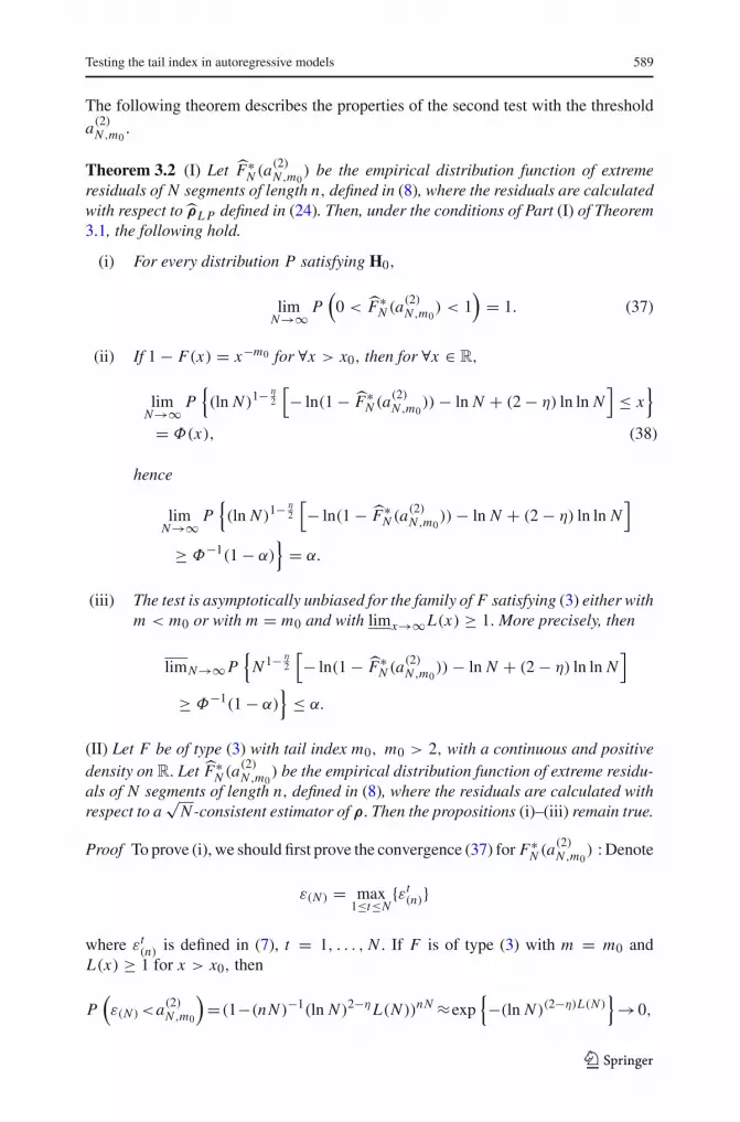
Testing the tail index in autoregressive models 589

The following theorem describes the properties of the second test with the thresholda(2)N ,m0

.

Theorem 3.2 (I) Let F∗N (a

(2)N ,m0

) be the empirical distribution function of extremeresiduals of N segments of length n, defined in (8), where the residuals are calculatedwith respect to ρL P defined in (24). Then, under the conditions of Part (I) of Theorem3.1, the following hold.

(i) For every distribution P satisfying H0,

limN→∞ P

(0 < F∗

N (a(2)N ,m0

) < 1)

= 1. (37)

(ii) If 1 − F(x) = x−m0 for ∀x > x0, then for ∀x ∈ R,

limN→∞ P

{(ln N )1− η

2

[− ln(1 − F∗

N (a(2)N ,m0

))− ln N + (2 − η) ln ln N]

≤ x}

= Φ(x), (38)

hence

limN→∞ P

{(ln N )1− η

2

[− ln(1 − F∗

N (a(2)N ,m0

))− ln N + (2 − η) ln ln N]

≥ Φ−1(1 − α)}

= α.

(iii) The test is asymptotically unbiased for the family of F satisfying (3) either withm < m0 or with m = m0 and with limx→∞L(x) ≥ 1. More precisely, then

limN→∞ P{

N 1− η2

[− ln(1 − F∗

N (a(2)N ,m0

))− ln N + (2 − η) ln ln N]

≥ Φ−1(1 − α)}

≤ α.

(II) Let F be of type (3) with tail index m0, m0 > 2, with a continuous and positivedensity on R. Let F∗

N (a(2)N ,m0

) be the empirical distribution function of extreme residu-als of N segments of length n, defined in (8), where the residuals are calculated withrespect to a

√N-consistent estimator of ρ. Then the propositions (i)–(iii) remain true.

Proof To prove (i), we should first prove the convergence (37) for F∗N (a

(2)N ,m0

) : Denote

ε(N ) = max1≤t≤N

{εt(n)}

where εt(n) is defined in (7), t = 1, . . . , N . If F is of type (3) with m = m0 and

L(x) ≥ 1 for x > x0, then

P(ε(N ) <a(2)N ,m0

)=(1−(nN )−1(ln N )2−ηL(N ))nN ≈exp

{−(ln N )(2−η)L(N )}→0,

123

590 J. Jurecková et al.

as N → ∞. Similarly, if F is ultimately heavier than Pareto with m < m0, then

P(ε(N ) < a(2)N ,m0

)=

[1 −

(nN (ln N )2−η)− m

m0 L(N )]Nn → 0, as N → ∞.

The fact that F∗N (aN ,m0) > 0 with probability tending to 1 for the whole hypothesis is

obvious. Hence, P(

0 < F∗N (a

(2)N ,m0

) < 1)

→ 1, and finally we obtain (38) with the

aid of (12).Analogously as in the proof of Theorem 3.1, we conclude that with probability

tending to 1 not all residuals εt(n) are less than a(2)N ,m0

.

(ii) By the embedding theorem of Komlós et al. (1975), there is a sequence of inde-pendent Brownian bridges BN , N = 1, 2, . . . , such that

F∗N (a

(2)N ,m0

)− F∗(a(2)N ,m0) = N− 1

2 BN (1 − F∗(a(2)N ,m0))+ O

(N−1 ln N

)

= Op

(N−1(ln N )1− η

2 L12 (N )

)+ O

(N−1 ln N

). (39)

If m = m0 and L(x) ≥ 1 for x > x0, then it follows from (29) and from (39) that,

(ln N )1− η2

[− ln(1 − F∗

N (a(2)N ,m0

))+ ln(1 − F∗N (a

(2)N ,m0

))]

= (ln N )1− η2

{− ln

[1 − F∗

N (a(2)N ,m0

)

1 − F∗N (a

(2)N ,m0

)− 1 + 1

]}

= (ln N )1− η2 (1 − F∗

N (a(2)N ,m0

))−1[

F∗N (a

(2)N ,m0

)− F∗N (a

(2)N ,m0

)]

+Op

((ln N )−1+ η

2

)

= (ln N )1− η2

1 − F∗(a(2)N ,m0)

1 − F∗N (a

(2)N ,m0

)

(1 − F∗(a(2)N ,m0

))−1

op

(N−1(ln N )1− η

2

)

+Op

((ln N )−1+ η

2

)

= op

((ln N )1− η

2 −2+η+1− η2 (L(N ))−1

)+ Op

((ln N )−1+ η

2

)= op(1).

Moreover,

(ln N )1− η2

[− ln(1 − F∗

N (a(2)N ,m0

))− ln N + (2 − η) ln ln N]

= (ln N )1− η2

[− ln(1 − F∗

N (a(2)N ,m0

))+ ln(1 − F∗(a(2)N ,m0))

]

= (ln N )1− η2

{− ln

[1 − F∗

N (a(2)N ,m0

)

1 − F∗(a(2)N ,m0)

− 1 + 1

]}

= (ln N )1− η2

F∗N (a

(2)N ,m0

)− F∗(a(2)N ,m0)

1 − F∗(a(2)N ,m0)

+ Op

((ln N )−1+η) (40)

123

Testing the tail index in autoregressive models 591

If F has exactly the Pareto tail with m = m0, then

(ln N )1− η2 (1 − F∗(a(2)N ,m0

))−1 N− 12 BN (1 − F∗(a(2)N ,m0

)) →d N (0, 1) as N → ∞(41)

while the left-hand side of (40) is ultimately stochastically smaller than that of (41) ifm = m0 and L(x) ≥ 1 for x > x0. The rest of the proof is analogous to the proof ofTheorem 2.1 in Jurecková, and Picek (2001). ��

4 Consistency considerations

Let 1 − F(x) = x−m L(x), for x ≥ x0 > 0, with m > m0, let F∗(x) = F N (x) be thejoint distribution function of the maximal innovations {εt

(n), t = 1, . . . , N }, and F∗N

their empirical distribution function. Then

1 − F∗(a(1)N ,m0) ≤ n

(a(1)N ,m0

)−mL(N ) = N

−(1−δ) mm0 L1(N )

and N (1 − F∗N (a

(1)N ,m0

)) has the binomial distribution B(N , pN ) with

pN = 1 − F∗(a(1)N ,m0) ≤ N

−(1−δ) mm0 L1(N ).

Hence, E[N 1−δ(1 − F∗N (a

(1)N ,m0

))] = O

(N

−(1−δ)(

mm0

−1)

L1(N )

)and

Nδ2

(− ln(1 − F∗

N (a(1)N ,m0

))− (1 − δ) ln N)

= Op

(N

δ2 ln N (1 − δ)

(m

m0− 1

)L2(N )

)→ ∞. (42)

Thus, for the white noise sequence with the null autoregression we would reject thehypotheses H0, H1 with probability tending to 1. An analogous statement holds for1 − F∗

N (λa(1)N ,m0) with any fixed λ, 0 < λ < 1.

Let now F be concentrated on the positive half-axis and let F∗N be the empirical

distribution function of the maximal residuals {εt(n), t = 1, . . . , N } with respect to

linear programming estimator ρL P defined in (24). Then it follows from (24) to (28)and from (5) that

εt − Y′t−1(ρL P − ρ) ≥ 0, t = 1, . . . , nN ,

max1≤t≤nN

|Y′t (ρL P − ρ)| = Op (L(N )) = op(aN ,m0),

0 ≤ ε t(n) = max

1≤i≤nε(t−1)n−p+i ≤ max

1≤i≤nε(t−1)n−p+i +Op (L(N )) , t = 1, 2, · · · , N.

123

592 J. Jurecková et al.

This in turn implies that, given an 0 < η < 1, there exists N0 such that for N > N0,

under Pm, m > m0,

P{

1 − F∗N (a

(1)N ,m0

) ≤ 1 − F∗N (λa(1)N ,m0

)}

≥ 1 − η,

for any fixed λ, 0 < λ < 1, and this together with (42) and the following remarkimplies that we reject the hypothesis H0 with probability at least 1 − η for N > N0.

Analogous consideration applies to the hypothesis H1 with hypothetical m0 > 2,when the innovation distribution, possibly extended on the whole R

1, satisfies 1 −F(x) = x−m L(x) with m > m0 and with L(·) slowly varying at infinity; then ρ isestimated either by GM- or by GR-estimator.

5 Simulation study

We study the performance of the test on the Pareto tail index of the innovation distri-bution in the autoregressive model on the following three simulated time series:

(A) Xt = 0.05Xt−1 + εt , t = 1, 2, . . . , Nn,(B) Xt = 0.9Xt−1 + εt , t = 1, 2, . . . , Nn,(C) Xt = 0.6Xt−1 − 0.3Xt−2 + 0.2Xt−3 + εt , t = 1, 2, . . . , Nn,

with the following innovation distributions:

Pareto F(x) = 1 − ( 1x

)m, x ≥ 1.

Inverse normal F(x) ={

2(

1 −Φ(

1√x

))x > 0

0 x ≤ 0

Student f (x) = 1√mB

(12 ,

m2

)(

1 + x2

m

)−(m+1)/2, x ∈ R.

For each of these cases, the time series were simulated of the lengthsnN = 200 and 1, 000. (The initial values for the time series were obtained as the lastvalues of auxiliary simulated time series of length 500 with the same autoregressioncoefficients and innovation distribution and initial values 0.)The computation procedure for each of the above innovation distributions and timeseries was as follows:

(1) the autoregressive time series X1, . . . , Xn, Xn+1, . . . , X2n, . . . , X Nn was gen-erated;

(2) ρ was estimated by ρ (either Feigin and Resnick or Huber M-estimators);(3) residuals εt := Xt − ρ′

N Yt−1, t = 1 − p, 2 − p, . . . , nN were computed;

(4) the maxima ε(1)n , . . . , ε(N )n of the segments were found and the corresponding

empirical distribution function F∗N calculated;

(5) a decision was made about H0 or H1, respectively, based on F∗N (aN ,m0), with

a(1)N ,m0= (

nN 1−δ) 1m0 and a(2)N ,m = (

nN (ln N )−2+η) 1m , respectively.

(6) The step (5) was repeated for various values m0, δ, η;(7) the steps (1)–(6) were repeated 1, 000 times.

123

Testing the tail index in autoregressive models 593

Table 1 Numbers of rejections of the null hypothesis among 1,000 tests at level α = 0.05 for a(1)N ,m =(

nN 1−δ)1m and some selected values of m0; N = 50, n = 4, δ = 0.1

Distribution of white noise Time series m0 = 0.25 m0 = 0.4 m0 = 0.5 m0 = 0.6 m0 = 0.75

Pareto m = 0.5 A 987 675 244 38 0

B 987 675 244 38 0

C 987 675 244 38 0

Inverse normal A 990 736 320 79 1

B 990 736 320 79 1

C 990 736 320 79 1

m0 = 0.5 m0 = 0.8 m0 = 0.9 m0 = 1.0 m0 = 1.2

Pareto m = 1 A 992 674 439 246 35

B 992 674 441 246 36

C 992 674 439 245 36

m0 = 2.0 m0 = 2.5 m0 = 2.75 m0 = 3.0 m0 = 3.5

Student m = 3 A 867 569 402 255 66

B 865 565 398 254 63

C 866 564 403 251 69

Table 1 gives numbers of rejections of H0 or H1, respectively, among 1,000 tests at

level α = 0.05 for some selected values m0 and under a(1)N ,m = (nN 1−δ) 1

m ; δ =0.1, n = 4, N = 50. Similarly, Table 2 gives numbers of rejections under a(2)N ,m =(nN (ln N )−2+η) 1

m ; η = 0.1, n = 4, N = 50.

Remark 1 Notice that the Pareto and Student distributions with tail index m satisfyH0 (or H1) for m0 = m + ε, ∀ε > 0; the inverse normal distribution satisfies H0 (orH1) for m0 = 0.5 + ε, ∀ε > 0.

Remark 2 We see that the performance of the test practically depends only on the whitenoise and not on the structure of AR series (the time series A, B, C were generatedwith the same innovations values under a given distribution).

The frequencies of rejection of H0 or H1 under the Pareto distribution are plottedagainst m0 in Figs. 1 and 2. Because of the small difference in behavior between theseries A, B, C, the illustrations are made only for B.

The following Tables 3 and 4 and Figs. 3, 4 illustrate the influence of the choiceof δ on the frequency of rejections of the null hypothesis under some fixed values ofm0. The shape of the graph under m0 close the true m is rather typical. The situationis similar for the choice of η.

123

594 J. Jurecková et al.

Table 2 Numbers of rejections of the null hypothesis among 1,000 cases at level α = 0.05 for a(2)N ,m =(

nN (ln N )−2+η)1m ; N = 50, n = 4, η = 0.1

Distribution of white noise Time series m0 = 0.3 m0 = 0.4 m0 = 0.5 m0 = 0.52 m0 = 0.6

Pareto m = 0.5 A 1000 995 83 16 0

B 1000 995 83 16 0

C 1000 995 83 16 0

Inverse normal A 1000 1000 363 158 1

B 1000 1000 363 158 1

C 1000 1000 363 158 1

m0 = 0.8 m0 = 0.9 m0 = 1.0 m0 = 1.02 m0 = 1.1

Pareto m = 1 A 995 645 84 37 1

B 995 645 84 38 1

C 995 645 84 38 1

m0 = 2.5 m0 = 2.8 m0 = 3.00 m0 = 3.05 m0 = 3.5

Student m = 3 A 982 684 283 186 7

B 983 680 282 193 4

C 982 685 281 187 5

m_0

reje

ctio

n

0.0 0.5 1.0 1.5 2.0

020

040

060

080

010

00

m_0

reje

ctio

n

0.0 0.5 1.0 1.5 2.0

020

040

060

080

010

00

Fig. 1 Number of rejections of H0 (α = 0.05) plotted against m0 for Xt = 0.9Xt−1 + εt and a(1)N ,m =(

nN 1−δ)1m ; εt , t = 1, . . . , nN have the Pareto distribution with m = 0.5 (left) and m = 1 (right);

N = 50, n = 4, δ = 0.1 (solid), δ = 0.5 (dotted)

6 Application to the Czech daily maximum temperatures

The tests described above are applied to a 40-years dataset of daily maximum temper-atures measured at three meteorological stations in Czech Republic, over the period1961–2000. The names and coordinates of the three stations are as follows:

Praha-Ruzyne: 50◦06′N , 14◦15′E, altitude 364 m above sea level;Liberec: 50◦46′N , 15◦01′E, altitude 398 m above sea level;Brno-Turany: 49◦09′N , 16◦42′E, altitude 241 m above sea level.

123

Testing the tail index in autoregressive models 595

m_0

num

ber

of r

ejec

tion

0.0 0.2 0.4 0.6 0.8 1.0

020

040

060

080

010

00

m_0

num

ber

of r

ejec

tion

0.0 0.5 1.0 1.5 2.0

020

040

060

080

010

00

Fig. 2 Number of rejections of H0 (α = 0.05) plotted against m0 for Xt = 0.9Xt−1 + εt and a(2)N ,m =(

nN (ln N )−2+η)1m ; εt , t = 1, . . . , nN have the Pareto distribution with m = 0.5 (left) and m = 1

(right); N = 200, n = 5, η = 0.1

Table 3 Numbers of rejections of the null hypothesis among 1,000 cases for various δ under some m0;α = 0.05, N = 50, n = 4

Distribution of white noise δ

m0 0.01 0.1 0.2 0.3 0.4 0.5 0.6

Pareto m = 1 0.5 995 987 977 1000 1000 1000 1000

0.9 551 422 233 401 404 272 281

1.0 339 211 114 176 132 35 55

Pareto m = 3 2.5 786 694 589 812 894 925 997

2.9 591 512 390 616 727 787 966

3.0 553 469 333 566 681 747 943

Student m = 5 3.5 815 700 535 700 739 686 863

4.0 95 48 15 30 33 29 87

5.0 27 6 0 6 11 6 35

Table 4 Numbers of rejections of the null hypothesis among 1,000 cases for various δ under some m0;α = 0.05, N = 200, n = 5

Distribution of white noise δ

m0 0.01 0.1 0.2 0.3 0.4 0.5 0.6

Pareto m = 1 0.5 1000 998 1000 1000 1000 1000 1000

0.9 621 440 551 504 482 630 718

1.0 349 251 240 126 73 105 117

Pareto m = 3 2.5 828 706 877 903 957 1000 1000

2.9 567 408 548 574 688 924 998

3.0 483 327 459 487 596 879 995

Student m = 5 3.5 921 828 931 928 928 982 992

4.0 56 11 3 2 0 0 0

5.0 6 1 0 0 0 0 0

123

596 J. Jurecková et al.

delta

num

ber

of r

ejec

tion

H_0

0.0 0.2 0.4 0.6

020

040

060

080

010

00

Fig. 3 Number of rejections of H0 plotted against δ; α = 0.05, n = 5, N = 200 and Xt = 0.9Xt−1 +εt ;εt , t = 1, . . . , 1, 000 have Pareto distribution (m = 1), m0 = 0.5 (solid), m0 = 0.9 (dotted), m0 = 1.0(dashed)

delta

num

ber

of r

ejec

tion

H_0

0.0 0.2 0.4 0.6

020

040

060

080

010

00

Fig. 4 Number of rejections of H0 plotted against δ; α = 0.05, n = 5, N = 200 and Xt = 0.9Xt−1 +εt ;εt , t = 1, . . . , 1, 000 have Pareto distribution (m = 3), m0 = 2.5 (solid), m0 = 2.9 (dotted), m0 = 3.0(dashed)

The maximum temperatures were centered and deseasonalized by subtracting theaverage maximum temperature computed over the 40 years. The residuals then weremodeled as autoregressive series of order p = 1 (see Hallin et al. 1997).

Table 5 gives results of testing for all three time series for some selected values

m0 and under a(1)N ,m = (nN 1−δ) 1

m ; δ = 0.1, n = 5. Similarly, Table 6 gives the

conclusions under a(2)N ,m = (nN (ln N )−2+η) 1

m ; η = 0.1, n = 5.Hence, describing the summer temperatures residuals as an autoregressive series,

we could work with a heavy-tailed distribution. The results of tests indicate any smallinfluence of the location of the station. The tests can be also used to estimate the tailindex in the Hodges-Lehmann manner (see Jurecková, and Picek 2004).

123

Testing the tail index in autoregressive models 597

Table 5 Rejection (R) and non-rejection (N ) of the null hypothesis at level α = 0.05 for a(1)N ,m =(

nN 1−δ)1m and some selected values of m0; n = 5, δ = 0.1

Time series m0 = 3.2 m0 = 3.3 m0 = 3.5 m0 = 3.6 m0 = 3.7

Praha R N N N N

Liberec R R N N N

Brno R R R R N

Table 6 Rejection (R) and non-rejection (N ) of the null hypothesis at level α = 0.05 for a(2)N ,m =(

nN (ln N )−2+η)1m ; and some selected values of m0; n = 5, η = 0.1

Time series m0 = 2.5 m0 = 2.6 m0 = 2.65 m0 = 2.7 m0 = 2.75

Praha R R N N N

Liberec R R R R N

Brno R R R R N

Acknowledgments The authors thank the referee for having read the paper carefully and for makingconstructive suggestions.

References

Brockwell, P. J., Davis, R. A. (1991). Time series: theory and methods. (2nd ed.). New York: Springer.Castillo, E., Calambos, J., Sarabia, J. M. (1989). The selection of the domain of attraction of an extreme

value distribution from a data set. In J. Hüsler, R.-D. Reiss (Eds.), Extreme value theory—Proceedingsof Oberwolfach 1987. Lecture Notes in Statistics, vol. 51 (pp. 181–190). New York, Springer.

Embrechts, P., Klüppelberg, C., Mikosch, T. (1997). Modelling of extremal events in insurance and finance.New York: Springer.

Falk, M. (1995a). On testing the extreme value index via the POT-method. Annals of Statistics, 23,2013–2035.

Falk, M. (1995b). LAN of extreme order statistics. Annals of Institute of Statistical Mathematics, 47,693–717.

Feigin, P. D., Resnick, S. I. (1994). Limit distributions for linear programming time series estimators.Journal of Stochastic Processes & Applications, 51, 135–165.

Fialová, A., Jurecková, J., Picek, J. (2004). Estimating Pareto tail index using all observations. REVSTAT2(1), 75–100.

Galambos, J. (1982). A statistical test for extreme value distribution. In B. V. Gnedenko et al. (Eds.),Non-parametric statistical inference (pp. 221–230). Amsterdam: North Holland.

Gomes, M. I. (1989). Comparison of extremal models through statistical choice in multidimensionalbackground. In J. Hüsler, R.-D. Reiss (Eds.), Extreme value theory—Proceedings of Oberwolfach1987. Lecture Notes in Statistics, vol. 51 (pp. 191–203). New York: Springer.

Gomes, M. I., Alpuim, M. T. (1986). Inference in a multivariate generalized extreme value model—asymp-totic properties of two test statistics. Scandinavian Journal of Statistics, 13, 291–300.

Hallin, M., Jurecková, J., Kalvová, J., Picek, J., Zahaf, T. (1997). Non-parametric tests in AR models withapplications to climatic data. Environmetrics, 8, 651–660.

Hasofer, A. M., Wang, Z. (1992). A test for extreme value domain of attraction. Journal of the AmericanStatistical Association, 87, 171–177.

123

598 J. Jurecková et al.

Hosking, J. R. M. (1984). Testing whether the shape parameter is zero in generalized extreme value distri-bution. Biometrika, 71, 367–374.

Jurecková, J. (1999). Tests of tails based on extreme regression quantiles. Statistics & Probability Letters,49, 53–61.

Jurecková, J., Picek, J. (2001). A class of tests on the tail index. Extremes, 4(2), 165–183.Jurecková, J., Picek, J. (2004). Estimates of the tail index based on nonparametric tests. In M. Hubert,

G. Pison, A. Struyf, S. Van Aelst (Eds.), Statistics for industry and technology (pp. 141–152). Basel:Birkhäuser.

Komlós, J., Major, P., Tusnády, G. (1975). An approximation of partial sums of independent R.V.’s and thesample DF. Zeitschrift für Wahrscheinlichkeitstheorie und verwandte Gebiete, 32, 111–131.

Koul, H. L. (2002). Weighted empirical processes in dynamic nonlinear models. Lecture Notes in Statistics,166.

Marohn, F. (1994). On testing exponential and Gumbel distribution. In J. Galambos et al. (Eds.), Extremevalue theory (pp. 159–174). Dordrecht: Kluwer.

Marohn, F. (1998a). Testing the Gumbel hypothesis via the POT-method. Extremes, 1, 191–213.Marohn, F. (1998b). An adaptive efficient test for Gumbel domain of attraction. Scandinavian Journal of

Statistics, 25, 311–324.van Montfort, M. A. J., Gomes, M. I. (1985). Statistical choice of extremal models for complete and censored

data. Journal of Hydrology, 77, 77–87.van Montfort, M. A. J., Witter, J. V. (1985). Testing exponentially against generalized Pareto distribution.

Journal of Hydrology, 78, 305–315.Picek, J., Jurecková, J. (2001). A class of tests on the tail index using the modified extreme regression

quantiles. In J. Antoch, G. Dohnal (Eds.), ROBUST’2000 (pp. 217–226). Prague: Union of CzechMathematicians and Physicists.

Stephens, M. A. (1977). Goodness-of-fit for the extreme value distribution. Biometrika, 64, 583–588.Tiago de Oliveira, J. (1984). Univariate extremes: Statistical choice. In J. Tiago de Oliveira (Ed.), Statistical

extremes and applications (pp. 91–107). Dodrecht: Reidel.

123