arX

iv:a

stro

-ph/

0408

183v

1 1

0 A

ug 2

004

The AGASA/SUGAR Anisotropies and TeV Gamma Rays from

the Galactic Center: A Possible Signature of Extremely

High-energy Neutrons

Roland M. Crocker1,2, Marco Fatuzzo3, Randy Jokipii4, Fulvio Melia5

and Raymond R. Volkas2

1 Harvard-Smithsonian Center for Astrophysics

60 Garden St., Cambridge MA 02138

rcrocker@cfa.harvard.edu

2Research Centre for High Energy Physics, School of Physics,

The University of Melbourne, 3010 Australia

r.crocker, r.volkas@physics.unimelb.edu.au

3Physics Department,

Xavier University, Cincinnati, OH 45207

fatuzzo@cerebro.cs.xu.edu

4Department of Planetary Sciences,

The University of Arizona, Tucson, AZ 85721

jokipii@lpl.arizona.edu

5Physics Department and Steward Observatory,

The University of Arizona, Tucson, AZ 85721

melia@physics.arizona.edu

ABSTRACT

Recent analysis of data sets from two extensive air shower cosmic ray detec-

tors shows tantalizing evidence of an anisotropic overabundance of cosmic rays

towards the Galactic Center (GC) that “turns on” around 1018 eV. We demon-

strate that the anisotropy could be due to neutrons created at the Galactic Center

through charge-exchange in proton-proton collisions, where the incident, high en-

ergy protons obey an ∼ E−2 power law associated with acceleration at a strong

shock. We show that the normalization supplied by the gamma-ray signal from

EGRET GC source 3EG J1746-2851 – ascribed to pp induced neutral pion decay

at GeV energies – together with a very reasonable spectral index of 2.2, predicts a

neutron flux at ∼ 1018 eV fully consistent with the extremely high energy cosmic

– 2 –

ray data. Likewise, the normalization supplied by the very recent GC data from

the HESS air-Cerenkov telescope at TeV energies is almost equally-well compat-

ible with the ∼ 1018 eV cosmic ray data. Interestingly, however, the EGRET and

HESS data appear to be themselves incompatible. We consider the implications

of this discrepancy. We discuss why the Galactic Center environment can allow

diffusive shock acceleration at strong shocks up to energies approaching the ankle

in the cosmic ray spectrum. Finally, we argue that the shock acceleration may

be occuring in the shell of Sagittarius A East, an unusual supernova remnant lo-

cated very close to the Galactic Center. If this connection between the anisotropy

and Sagittarius A East could be firmly established it would be the first direct

evidence for a particular Galactic source of cosmic rays up to energies near the

ankle.

Subject headings: acceleration of particles — cosmic-rays — radiation mecha-

nisms:nonthermal — supernova remnants

1. Introduction

The origin of cosmic rays (CRs) is one of the most important unsolved problems in

astrophysics. While it has long been speculated that diffusive shock acceleration of protons

and ions at shock fronts associated with supernova remnants (SNRs) is the mechanism likely

responsible for accelerating the bulk of high energy cosmic rays, definitive observational proof

has been elusive. Further, the conditions at almost all known SNRs seem not to promote

the acceleration of CRs beyond the ‘knee’ feature in the spectrum at ≃ 5 × 1015 eV. The

acceleration mechanism for CRs between the knee and the ‘ankle’ at few ×1019 eV therefore

seems to be an even deeper puzzle.

The purpose of this paper is to argue that the Galactic Center (GC), a region with

relatively extreme conditions compared to the rest of the Milky Way, is a likely site where

CRs are accelerated up to the ankle. Our argument is based on the following: (i) The

EGRET γ-ray source 3EG J1746-2851, most likely located near the GC, provides good

evidence for pion production from high energy proton-proton (pp) collisions. Neutrons will

then inevitably also be produced by this source. (ii) The TeV γ-rays from the direction of the

GC detected by a number of air Cerenkov telescopes, in particular, the HESS instrument,

also support the notion that high-energy proton acceleration and collision processes (again,

leading inevitably to neutron production) are occuring in this region. (iii) The AGASA CR

anisotropy for the energy range 1017.9 − 1018.5 eV is consistent with high energy neutron

emission from the GC. (iv) The reanalysed SUGAR data also reveal an anisotropy for this

– 3 –

energy regime from a direction close to the GC. (v) The SNR Sgr A East provides a plausible

specific GC system where hadronic acceleration up to the ankle can occur, differing as it does

from other Galactic SNRs by the special conditions of its GC environment.

If the connection between the anisotropies and Sgr A East could be firmly established,

it would be the first identification of a specific source producing high energy, Galactic CRs,

and, moreover, it would be proven to be an important, possibly unique, contributor to CR

acceleration up to the ankle. The southern-hemisphere AUGER detector, currently under

construction, will test our hypothesis in the relatively near future: it should see a significant

point source of ∼ 1018 eV neutrons at the GC. (For lower energies, previous work has

shown that a GC neutrino signal should also be seen by a northern-hemisphere km3 neutrino

telescope: Crocker et al. 2002).

We extend earlier work on GC CR production in three important ways. First, pos-

tulating a GC source of high energy protons obeying an ∼ E−2 power law at the source,

with normalisation fixed by the concomitant (GeV) EGRET γ-ray observations of 3EG

J1746-2851, we calculate neutron production through charge-exchange pp → nX reactions.

Quite non-trivially, we find neutron fluxes consistent with the magnitudes of the AGASA and

SUGAR anisotropies. Second, we likewise show that a simultaneous fit to the (TeV) data

supplied by the HESS instrument and the cosmic ray anisotropy data is also consistent with

the existence of a population of of shock-accelerated protons governed by a ∼ E−2 power law

up to extremely high energies. Third, we show that diffusive shock acceleration beyond the

knee can occur provided that there is a significant magnetic field component perpendicular

to the SNR shock propagation direction (i.e., parallel to the shock front). We explain why

the special conditions at the GC, especially the higher density of the ambient medium and

higher magnetic field, can realise this situation. Third, we argue that the specific GC SNR

Sgr A East is the most likely specific candidate site for CR acceleration up to the ankle. Note,

however, that it is not necessary to identify the specific source for the conclusion italicised

above to follow.

Note also that we admit from the start that our model is not consistent with all avail-

able data. The data, however, are inconsistent amongst themselves in the two important

instances where there is disagreement with our model (see §3.3 and §5.4). These instances

of disagreement – both discussed in further detail below – are (i) that the SUGAR results

indicate a point source offset by 7.5◦ from the GC (whereas we predict, of course, a source

at the position of the GC on the sky) and (ii) that the ∼ TeV measurements of the γ-ray

flux from the GC (by a number of instruments) appears to be deficient compared to what

we would expect. We discuss a number of possible resolutions of this discrepancy, finding

the most favorable to hinge on there being two effective GC sources of γ-rays, an idea which

– 4 –

has some support from current observations.

2. Origin of Cosmic Rays: Role of Neutrons

The hypothesis that shocks at SNRs are responsible for the acceleration of CRs over

the bulk of the observed spectrum is fifty years old (Shklovskii 1953). And, indeed, there is

strong, albeit circumstantial, evidence that SNRs do accelerate cosmic rays up to, at least,

the ‘knee’ in the spectrum at a few PeV (we set Eknee ≡ 1015 eV for definiteness). This

evidence comes primarily from two arguments, viz,

1. Supernovae seem to be the only class of Galactic object able to inject the power neces-

sary to maintain the observed cosmic ray output of about 1048 ergs/year (e.g., Longair

(1994)).

2. The cosmic ray spectrum is governed by a power law with spectral index around 2.7.

This is close to the universal power law of spectral index ∼ 2 theoretically expected

from diffusive shock acceleration at the sort of strong shock associated with a supernova

blast wave. (Note that this theoretical expectation for spectral indices close to two – at

the source – is observationally confirmed by radio and γ-ray data from various SNRs.)

The difference between these two indices, further, can be compellingly explained as

arising from energy-dependent propagation/confinement effects.

However, there is yet no direct observational evidence for the SNR-CR connection and

certainly no particular SNR has been proven to be a CR source. Further, many researchers

have found that their models are pushed to accelerate particles up to Eknee. This becomes

doubly troubling given the fact that, as emphasized by Jokipii and Morfill (1991), matching

the spectra at the knee requires, short of a cosmic conspiracy, that the population of cosmic

rays above the knee is closely related to that below the knee. In fact, there are good reasons

to think that the bulk of the cosmic rays are Galactic in origin up to the ‘ankle’ in the

spectrum at a few × 10 EeV (1 EeV ≡ 1018 eV), not the least of which is that a proton of

this energy has a gyroradius the size of the radius of the Galactic disk.1

We would like, therefore, to determine whether it is, indeed, the case that SNRs can

accelerate particles up to energies of 1018−19 eV. Further, it would be helpful to find evidence

1Yet higher energy CRs may therefore no longer be confined to our Galaxy, so are almost certainly extra-

Galactic. The up-turn in the spectrum at the ankle is nicely consistent with a new population taking over

from a diminishing Galactic component.

– 5 –

that some particular object is accelerating particles to these extremely high energies (EHEs).

We obviously need to look for a signal in electrically neutral particles, so that the

location of the source is not scrambled by deflection due to the Galactic magnetic field.2

There are three main candidates: photons, neutrinos and neutrons. Photons with energy

1017,18 eV will be produced by the decay of neutral pions produced by hadronic collisions.

However, such EHE γ’s will interact strongly with background media long before reaching

the Earth, so they are not useful as direct probes at those energies. The flux of 1017,18 eV

neutrinos, another concomitant of hadronic collisions, is expected to be orders of magnitude

too small to be seen by future km3 neutrino telescopes. Although three of us have previously

shown that the GC should emit neutrinos (Crocker et al. 2000; Crocker et al. 2002) [see also

(Alvarez-Muniz and Halzen 2002)], their detection could not settle the question of where the

1018 eV CRs are coming from, because the detectable flux of neutrinos lies at considerably

lower energies.

This leaves us with neutrons. As for neutrinos and γ-rays, neutrons are an inescapable

concomitant of hadronic acceleration of protons and ions: charge exchange occurs in a non-

negligible fraction of all interactions between accelerated protons and ambient protons. Neu-

trons are also produced in pγ collisions and dissociations of accelerated ions (see below). The

neutron, however, is unstable in free space, a fact we have to take into account when con-

templating neutron astronomy.

The neutron is the longest-lived unstable ‘elementary’ particle with a decay time at

rest, τn, of 886 seconds (Hagiwara and al. 2002). This means that a neutron will travel, on

average, a distance of

dn(En) = cγnτn ≃ 9

(

En

EeV

)

kpc, (1)

(where the Lorentz factor is given by γn ≡ En/mn) in free space before decaying. What

plausibly neutron-producing regions lie within the ∼ 9 kpc distance travelled on average by

an EeV neutron? The Galactic Center – one of the most energetic regions in the Galaxy –

at a distance of around 8.5 kpc is the principal candidate.

What would be a smoking gun signature for EHE CR neutrons? It is in extensive air-

showers (EAS) apparently initiated by particles coming from the direction of the GC that

one would need to look for GC neutrons. The signal might be very difficult to disentangle,

essentially because any neutron-initiated EAS at these energies is likely to be indistinguish-

2Charged particles can still be used for very close sources. See, for example, Chilingarian (2003) for a

study of putative CR emission from the 300 pc distant Monogem ring SNR.

– 6 –

able from a background, proton-initiated EAS3 (which proton, given the presence of the

Galactic magnetic field, might originate from a source considerably away from the GC). The

best evidence for GC neutrons one might hope for, then, is an anisotropy in the EeV cosmic

ray data in the form of an excess towards the GC. Intriguingly, there is tantalizing evidence,

which we now briefly review, from two different data sets that just such an anisotropy exists.

3. The Galactic Center Anisotropy Explained by a GC Source of

Protons/Neutrons

Recent analysis of data from two different cosmic ray detectors has revealed the presence

of an anisotropic overabundance of cosmic rays coming from the general direction of the

Galactic Center. Consistent with these findings, analysis of data from a third array has

found a broad anisotropy along the Galactic plane. We now briefly review each of these

findings.

Statistically, the most robust determination for an anisotropy has been by the Akeno

Giant Shower Array (AGASA) Group (Hayashida et al. 1999a) which, in analysis of 114,000

airshowers found a strong – 4% amplitude – anisotropy in the energy range 1017.9−1018.3 eV

(we label the 1017.9 eV energy at which the anisotropy apparently ‘turns on’ Eonset). Note that

the AGASA Collaboration (Takeda 1999) has estimated that the systematic uncertainty in

its instrument’s energy callibration is 30% and we shall adopt this figure in our analysis. The

group’s two-dimensional analysis of the data showed that this anisotropy could be interpreted

as an excess of air showers from two regions each of ∼ 20◦ extent, one of 4σ significance near

the GC and another of 3σ in Cygnus. Subsequent re-analysis by the AGASA group –

incorporating new data – has only served to bolster the claim that the anisotropy is real

(Hayashida and al. 1999b) with, this time, a 4.5 σ excess seen near the GC over a beam size

of 20◦ between 1018.0 − 1018.4 eV.

Prompted by the AGASA result, Bellido et al. (2001) re-analyzed the data collected

by the SUGAR cosmic ray detector which operated from 1968 to 1979 near Sydney. Set-

ting a priori an energy range similar to that determined for the AGASA anisotropy, these

researchers also found an anisotropy, consistent with a point source located at 7.5◦ from the

3Though note here that there is a theoretical possibility, at least, that empirical data may one day be

able to directly distinguish EHE cosmic ray neutrons from protons via characteristic differences between the

µ+ to µ− ratios seen in the extensive air showers generated by these particles (a proton will produce an

excess of π+ and, therefore, µ+ in the forward region whereas a neutron will produce an excess of π− and,

therefore, µ−).

– 7 –

GC – and 6◦ degrees from the AGASA maximum over an energy range of 1017.9 − 1018.5 eV.

Lastly, the HiRes Collaboration has seen a Galactic Plane enhancement in cosmic ray

events in the energy range between 1017.3 and 1018.5 eV with 3.2σ confidence (Bird et al. 1999)

(this is consistent with the AGASA and SUGAR results because the HiRes study was broad

scale and did not attempt to pin down whether any particular Galactic longitudes were

responsible for the detected excess: Bellido et al. 2001).

As we shortly set out, the anisotropies mentioned above have what we believe is a

natural explanation in terms of neutron emission from the GC region (see the subsection on

‘GC Neutron Models’ below). Before we discuss this idea in detail, however, we also consider

the possibility that the observed anisotropies can be explained directly by a diffusive flux of

charged particles from the GC. We label such scenarios ‘GC Charged Particle Models’.

3.1. GC Charged Particle Models

There has been a concerted effort to model the propagation of charged particles from

an assumed source in the vicinity of the GC, through various assumed configurations of the

Galactic magnetic field, to Earth to see whether these models can reproduce the observed

anisotropies (Clay 2000;Bednarek, Giller, and Zielinska 2002;Candia, Mollerach, and Roulet

2002). In general, researchers have found that a fair degree of correspondence between

models and reality can be achieved, with, in particular, an anisotropy becoming evident

for O[EeV] protons propagating through various field configurations with a magnetic field

amplitude of O[µG]. Finding an exact correspondence for ‘turn-on’ and ‘turn-off’ energies

seems, however, to require quite some fine-tuning of the particulars of BGalactic and is not

such a robust solution as the neutron idea. Further, for reasonable amplitudes of BGalactic

modeling studies show that the actual separation seen between the GC and the observed

excess will exceed the O[10◦] observed (Candia, Epele, and Roulet 2002). In fact, Medina-

Tanco and Watson (2001) report that the source must be within ∼ 2 kpc of the Earth to

reproduce the observed deflection. This is of course, a possibility, but then the near alignment

with the anisotropies and the GC becomes, essentially, a coincidence. Lastly, and perhaps

most tellingly, the (consistent with-) point-like anisotropy seen in the SUGAR data is very

difficult to reproduce in modeling of charged particle trajectories because the particles tend

to smear out until rather higher energies (for reasonable magnetic fields) than Eonset.

– 8 –

3.2. GC Neutron Models

The broad idea that neutron emission from the GC may produce an anisotropy was,

to our knowledge, first mooted by Jones (1990). The neutron idea was subsequently re-

vived by the AGASA group in the paper announcing their discovery of the GC anisotropy

(Hayashida et al. 1999a). The AGASA paper authors pointed out that the anisotropy ‘turn

on’ at a definite energy of ∼ EeV finds a natural explanation in the fact that – as outlined

above – this energy corresponds to a gamma factor for neutrons large enough that they can

reach us from the GC. So, broadly, neutrons below this energy decay in propagation and are

then diverted by Galactic magnetic fields. The cessation of the anisotropy above ∼ 1018.4

eV can be explained as either due to a very steep GC source spectrum or an actual cut-off

in the source so that the background takes over again at this energy.

Most recently, the broad idea above has been considerably refined in the work of Bossa

et al. (2003), whose basic scenario we follow and now explain. These authors have made

detailed propagation calculations following the trajectories of protons from neutrons that

decay in flight from the GC or, to be precise, they follow the trajectories of anti-protons

leaving the Earth and calculate the probability that a decay should occur over the interval

during which the anti-proton’s path points back to the assumed GC source. Using this

procedure they calculate detailed maps of the arrival direction of the combined neutron and

proton signal for various values of an assumed Galactic magnetic field which has both a

regular and a turbulent component. The Bossa et al. (2003) scenario extends that presented

by Medina-Tanco and Watson (2001) in which, essentially, decay protons produced close to

the Earth arrive from directions close to the GC whereas those produced in the inner Galaxy

arrive preferentially from the directions of the spiral arms – thus also neatly explaining the

Cygnus anisotropy – as their trajectories wind around the regular magnetic field lines (Bossa

et al. 2003).

Crucially, the GC, with declination δ = −28.9◦, is outside the field of view of AGASA

(which is limited to δ > −24◦; Bossa et al. 2003). This provides a natural explanation for

the ‘turn off’ of the AGASA anisotropy without the need for a source cut-off: at energies

& 1018.4 eV, neutrons do not (on average) decay in flight from the GC, but, instead, travel

in a straight line from the GC to Earth to produce a point-like anisotropy out of the field of

AGASA. Moreover, Bossa et al. (2003) were also able to reproduce the sharp onset of the

AGASA anisotropy at 1017.9 eV by positing a Galactic magnetic field random component

of fairly large amplitude (3 µG) and also assuming a GC source governed by a spectral

index of 2.2. As mentioned above, these researchers also relate the Cygnus region excess

seen by AGASA to the GC source with a Galactic magnetic field whose regular component

is along the spiral arms (and not just azimuthal). Finally, in the Bossa et al. (2003)

– 9 –

scenario, the magnitudes and morphologies of the AGASA and SUGAR results were shown

to be compatible (directional consistency being problematic – see below). In addition to

approximate consistency in magnitude, the fact that the AGASA and SUGAR anisotropies

are, respectively, diffuse and (consistent with) point-like finds a natural explanation. Indeed,

from the requirement that the source normalization generate the observed 4% amplitude

anisotropy of the right-ascension first harmonic (and continuing to assume a power-law source

spectrum with index 2.2), Bossa et al. (2003) determine that the total luminosity of the GC

source over the specified decade in energy be

LGC(1017.5 − 1018.5) ≃ 4 × 1036erg s−1 , (2)

which implies a direct neutron flux between 1017.9−1018.5 eV of 2×10−17 cm−2 s−1 (no error

range given), which is not very different from the SUGAR result of (9±3)×10−18 cm−2 s−1.

Bossa et al. (2003) also point out that these two figures need not be exactly equal: protons

will be, in general, delayed by many thousands of years with respect to the neutron arrival

times so the source intensity need not be exactly the same when the neutrons and protons

we observe today were separately emitted.

A couple of important points one should note about the Bossa et al. (2003) scenario (as

these researchers themselves remark) are that (i) for the magnetic field adopted, the phase

(∼ 330◦) of the first harmonic in right ascension found is somewhat larger than that detected

by AGASA and (ii) because Bossa et al. (2003) do relate the Cygnus excess to a GC source,

this excess should disappear for E & 2 EeV independently of the intrinsic source energy cut-

off because any reasonable Galactic magnetic field could not, reasonably, shepherd cosmic

rays above this energy along a spiral arm.

3.3. Non-coincidence of the SUGAR ansisotropy with the GC

That the AGASA ansisotropy is not exactly coincident with the GC finds a reasonable

explanation in the fact already presented that the actual GC is out of the field of view of

this instrument. That the SUGAR ansisotropy, however, is not coincident with the GC

presents a challenge to all scenarios that would posit that the source of the EHE cosmic

rays is at the GC. Either, then, all such scenarios are incorrect or the SUGAR directional

determination is somewhat in error. If not the GC, then the SUGAR anisotropy could be

due to the supernova remnant W28, which has also been detected by the EGRET instrument

in gamma rays. However, W28 (located at α = 274◦, δ = −23.18◦) is itself displaced from

the SUGAR position by about 4◦, and one would need to again invoke an error in SUGAR’s

directional determination. For reasons we immediately explain, such an error seems to be a

viable possibility for, if the SUGAR directional determination is correct then

– 10 –

1. in the case that the anisotropy is due to neutrons there must be a completely

unknown source at the position suggested by the SUGAR data (unobserved, e.g., by

the EGRET instrument in gamma rays)

2. or, alternatively, in the case that the anisotropy is due to protons directly

either

(a) there is a source located very close to us which is contrained to be in close but

completely coincidental alignment with the direction towards the GC

or

(b) there is a source somewhat further away, the particles produced by which – also

completely coincidentally – happen to be bent in flight in exactly such a way as

to appear to come from close to the direction of the GC (and, further, remain

sufficently bunched that their signal is consistent with point-like for SUGAR).

We note, furthermore, that whereas, as stressed above, the GC is outside the field of

view of AGASA, the position of the SUGAR maximum is inside the AGASA field of view

so that the putative SUGAR source should be seen by AGASA. That it is not means that

these two instruments are in disagreement. AGASA, moreover, has the better statistics.

We believe, then, that a quite natural reading of the situation is that SUGAR’s directional

determination is in error. The only other way out of this apparent dilemma is to posit

significant variability (between the SUGAR and AGASA observation times) at the source

which, however, would in fact be an argument in favor of a point source, rather than diffuse

emission.

4. Evidence for Hadronic Acceleration at the Galactic Center

Direct evidence of hadronic acceleration at the Galactic center comes from the EGRET

detection of a 30 MeV - 10 GeV continuum source (3EG J1746-2851 in the third EGRET

catalog: Hartman et al. (1999)) within 1◦ of the nucleus (Mayer-Hasselwander et al. 1998)4.

The EGRET spectrum exhibits a clear break at ∼ 1 GeV, and therefore cannot be fit by a

single power law. Instead, this break appears to be the signature of a process involving pion

decays. Specifically, the decay of neutral pions generated via pp scatterings between relativis-

tic and ambient protons produces a broad γ-ray feature that mirrors all but the lowest energy

4The IBIS telescope on board INTEGRAL has also recently released a preliminary result for the detection

of a GC source in the EGRET energy range: Di Cocco et al. (2004)

– 11 –

EGRET data. Of course, pp scatterings also produce charged pions which, in turn, decay

into “secondary” electrons and positrons. These leptons are capable of producing their own

γ-ray emission via bremsstrahlung and Compton scattering. Interestingly, if the secondary

leptons build up to a steady-state distribution balanced by bremsstrahlung and Coulomb

losses, the former accounts naturally for the lowest energy EGRET datum, independent of

the ambient proton number density. This crucial feature results from the fact that the sec-

ondary leptons produce a steady state distribution whose normalization scales as the inverse

of the ambient proton number density, whereas the bremsstrahlung emissivity per lepton

scales directly with this density. The pion decays link the lepton and photon generation

rates, so the bremsstrahlung and pion-decay photon emissivities are tightly correlated.

While this discussion is quite general in nature, it is important to note that Sgr A

East, a mixed-morphology SNR located within several parsecs of the Galactic center, is a

viable candidate for the site of hadronic acceleration (see § 7.2 for a more complete discus-

sion). Specifically, the observation of OH maser emission at the boundary of this structure

provides strong evidence for the presence of shocks (Yusef-Zadeh et al. 1996, 1999). In addi-

tion, Fatuzzo & Melia (2003) have found that a power-law distribution of shock-accelerated

relativistic protons injected into the high-density, strongly magnetized Sgr A East enviro-

ment leads to a pion-decay process (described above) that can account for both the EGRET

source 3EG J1746-2851 and the unique radio characteristics of Sgr A East. This scenario

may also account for the e+ − e− annihilation radiation observed from the galactic bulge by

the Oriented Scintillation Spectrometer Experiment (OSSE) aboard the Compton Gamma

Ray Observatory (Fatuzzo, Melia and Rafelski 2001).

Finally, further evidence for the occurence of hadronic acceleration at the Galactic center

is presented by the detection of this region at ∼ TeV energies by a number of air Cerenkov

telescopes: see §5.4 for more on this point.

5. Relating a Pion-Decay γ-ray flux to a Neutron Flux

The processes via which an impinging, EHE charged beam can lead to the production

of astrophysical neutrons can be summarized as (with the ‘beam’ particle indicated first in

each pair, the target second):

1. pp

2. Ap, A 6= p

3. pγ

4. Aγ, A 6= p.

– 12 –

In more detail, these processes are:

1. Leading neutron production from collisions of accelerated protons with ambient, target

protons.

2. Neutron production via dissociation of accelerated ions through collisions with ambient,

target protons.

3. Photo-production of leading neutrons (i.e., charge-exchange production of neutrons in

collisions of accelerated protons with ambient, target photons).

4. Photo-dissociation (fragmentation) of accelerated ions.

Of the existing work concerned with the GC anisotropy and its explanation in terms of

neutron production at various possible GC sites, the AGASA group’s anisotropy discovery

paper (Hayashida et al. 1999a) focused on the idea that the disintegration of accelerated

heavy ions by interactions with ambient matter or photons was the ultimate source of the

(putative) EHE neutrons. This follows the lines of the broad scenario investigated by Sikora

(1989) for active galactic nuclei in which the very same strong magnetic fields that serve to

accelerate charged particles to high energies also serve to confine the same to some central

accelerating region (whereas neutrons escape). Also of relevance here is the work of Tkaczyk

(1994).

Alternatively to the heavy-ion disintegration idea, Medina-Tanco and Watson (2001)

have proposed that a more likely method of EHE neutron production is via interactions be-

tween accelerated protons and ambient protons or IR γ’s. They found that the environment

of Sgr A∗ – the supermassive black hole at the GC – is sufficiently dense that the particle

interaction rate required to produce the desired neutron flux is achievable. We shall have

more to say about this scenario below.

Takahashi and Nagataki (2001) also considered neutron production and determined that

it is pp interactions which most effectively produce the required neutrons. For reasons we

shall explain below, we agree with this conclusion (though our calculations differ importantly

in specifics). Takahashi and Nagataki (2001) also researched the detectability of neutrinos

concomittant with neutron production. More recently, Anchordoqui et al. (2003) have

studied the detectability of neutrinos produced in the decay-in-flight of the (putative) GC

neutron beam and Biermann et al (2004) have considered a model in which the observed

anisotropy is explained as due to the last GRB to go off in the Galaxy.

– 13 –

5.1. Detailed Calculation of Neutron Flux from pp Collisions

Protons accelerated to relativistic energies at the GC source can undergo a series of inter-

actions including pN → pN mmeson mNN , where N is either a p or a neutron n, mmeson denotes

the energy-dependent multiplicity of mesons (mostly pions), and mNN is the multiplicity of

nucleon/anti-nucleon pairs (both increasing functions of energy). Since mNN/mmeson < 10−3

at low energy and even smaller at higher energies (Cline 1988), following Markoff et al.

(1997) we here ignore the anti-nucleon production events. The charge exchange interaction

(p → n) occurs around 40% of the time at accelerator energies and this fraction is predicted

to be only very weakly energy-dependent (see the appendix). We shall take it, then, that

the leading neutron multiplicity, mn, is given by a fixed proportion of 0.4 (i.e., 40% of all pp

interactions involve charge exchange, independent of incoming proton energy).

Other possible interactions of accelerated p’s – all potentially important for cooling –

are pγ → pπ0γ, pγ → nπ+γ, pγ → e+e−p and pe → eNmmeson (Markoff et al. 1997).

5.1.1. The production of π0 decay photons

The (differential) π0 emissivity resulting from an isotropic distribution of shock acceler-

ated protons dnp(Ep)/dEp (where [dnp(Ep)/dEp] is in units of cm−3 eV−1) interacting with

cold (fixed target) ambient hydrogen of density nH is given by the expression

Qppπ0(Eπ0) = c nH

∫

Ethp (E

π0 )

dEpdnp(Ep)

dEp

dσ(Eπ0, Ep)

dEπ0

, (3)

where Ethp (Eπ0) is the minimum proton energy required to produce a pion with total energy

Eπ0 (determined through kinematical considerations) and [Qppπ0 ] = pions s−1 cm−3 eV−1. The

resulting γ-ray emissivity is then given by the expression

Qγ(Eγ) = 2

∫

Emin

π0(Eγ)

dEπ0

Qppπ0(Eπ0)

(E2π0 − m2

π0)1/2, (4)

where Eminπ0 (Eγ) = Eγ + m2

π0/(4Eγ).

At proton energies, Ep, greater than ∼ 5 GeV—above the ∆ resonance-affected region—

the differential cross-section is approximated by the scaling form of Blasi & Melia (2003; see

also Blasi & Colafrancesco 1999):

dσ(Ep, Eπ0)

dEπ0

=σ0

Eπ0

fπ0(x0) , (5)

– 14 –

where x0 ≡ Eπ0/Ep, σ0 = 32 mbarn, and (Hillas 1980)

fπ0(x0) = 0.67(1 − x0)3.5 + 0.5e−18x0 . (6)

This scaling form properly takes into account the high pion multiplicities which occur at

high energies.

Given the above and a parent proton distribution governed by a power law, dnp(Ep)/dEp

with spectral index γ,dnp(Ep)

dEp∝ E−γ

p (7)

we can write the neutral pion emissivity due to pp as

Qppπ0(Eπ0) =

dnp(Eπ0)

dEp

σ0 nHc Λ0(γ) , (8)

and, consequently, the photon emissivity due to the decay of these π0’s as

Qγ(Eγ) ≃ cnH

∫ ∞

Eγ

dEπ0

∫ ∞

Eπ0

dEpdnp(Ep)

dEp

dσ(Ep, Eπ0)

dEπ0

2

Eπ0

≃ 2

γ

dnp(Eγ)

dEpσ0 nHc Λ0(γ) ,

(9)

where in both equations immediately above we employ

Λ0(γ) ≡∫ 1

0

dx0 xγ−20 fπ0 = 2

{

Γ(γ − 1)

[

181−γ +15.5865

Γ(3.5 + γ)

]

− E(2 − γ; 18)

}

, (10)

in which Γ(x) is the Euler Gamma function and E(n; z) is the exponential integral function

which satisfies E(n; z) ≡∫ ∞

1exp(−zt)/tn dt.

5.1.2. The Production of Neutrons in the Scaling Regime

Similarly to the above, the emissivity of neutrons from an isotropic distribution of shock

accelerated protons dnp(Ep)/dEp interacting with cold (fixed target) ambient hydrogen of

density nH is given by the expression

Qppn (En) = c nH

∫

Ethp (En)

dEpdnp(Ep)

dEp

dσ(En, Ep)

dEn. (11)

To proceed further we would like to take, in analogy to the above,

dσ(Ep, En)

dEn=

σ0

Enfn(xn) , (12)

– 15 –

where xn ≡ En/Ep. We must now determine an expression for fn(xn). In this regard, we

employ the formalism set out in Appendix A of Drury et al. (1994). Following Gaisser

(1990), this reference sets out the calculation of the ‘spectrum-weighted moment’ (SWM),

denoted by 〈mxS〉γS, for the emission spectrum of various particle species (labeled by S) from

collisions of protons from a power-law distribution equation (7) and where xS ≡ ES/Ep. In

this formalism, the emissivity of species S can be written

QS(ES) =dnp(ES)

dEpσppnHc〈mx〉γS, (13)

so that we see that Λ0(γ) defined in equation (10) above is nothing but the SWM for neutral

pions produced in pp collisions.

Drury et al. (1994) provide their own calculation of the SWM for neutral pions, decay

gammas, and neutrons (〈mx〉γπ0 , 〈mx〉γγ, and 〈mx〉γn). We set out their results and ours

(calculated with the fπ0 given above) for comparison for pions and pion decay gammas in

Table 1.

To arrive at a SWM for neutron production calculations, Drury et al. (1994) employ

the dimensionless, inclusive cross-section for neutron production given by Jones (1990), viz

gn(xn) = nn(αn + 1)(1 − xn)αn . (14)

Jones (1990) gives, on the basis of his analysis of 300 GeV proton collider data, αn = 2,

and an average neutron multiplicity, nn, of 0.25. We adopt his results excepting the neutron

multiplicity which we revise to be 0.4: see the appendix for more detail on this issue. We

find, then, that

gn(xn) → 1.2(1 − xn)2. (15)

The translation of this distribution into our formalism is simply

fn(xn) ≡ xngn(xn) = 1.2xn(1 − xn)2. (16)

We find, then,

Qppn (En) ≃ c nHσ0

dnp(En)

dEp

Λn(γ) , (17)

where we have defined

Λn(γ) ≡∫ 1

0

dxn xγ−2n fn(xn) = 2.4

1

γ(γ + 1)(γ + 2). (18)

– 16 –

γ 2.0 2.2 2.4 2.6

Λ0(γ) 0.177 0.113 0.076 0.053

〈mx〉γπ0 0.17 0.092 0.066 0.048

Λn(γ) 0.177 0.103 0.063 0.041

〈mx〉γn 0.19 0.094 0.051 0.030

Table 1: Values of Λ(γ) for both neutral pions and neutrons from pp collisions compared to

the spectrum-weighted distributions for same calculated in Drury et al. (1994).

5.1.3. Relating Photon and Neutron Emissivity and Fluxes in the Scaling Regime

Now, from Eqs.(9) and (17) we have that

Qppn (En) = 0.8γ

Λn(γ)

Λ0(γ)Qγ(E

0γ)

(

En

E0γ

)−γ

, (19)

where we have also used the fact that both daughter γ and neutron spectra will be governed

by the same power law as the parent protons. We have, then, related the neutron emissivity

at some energy En to the photon emissivity at a normalization energy E0γ (assuming scaling

holds). We present (0.8γΛn[γ])/Λ0[γ] for various values of the spectral index γ in Table 2.

The growth of this ratio with energy can be related to the fact that, because the average

energy of a neutron produced in a pp interaction (at lab energy Ep) will be higher than the

energy of a pion-decay γ produced (indirectly) by a pp interaction at the same energy (Ep),

the neutron flux at En is ‘directly’ tied to the photon flux at a somewhat lower energy. This

means that as one steepens a spectrum – thereby increasing the number of photons in the

population below some fixed pivot point (at which the normalization is effected) – one also

tends to increase the population of neutrons at En.

Note that in employing the relation set out in equation (19), careful attention should

be paid to the following points:

1. The neutron emissivity is related not to the total photon emissivity but, rather, related

to that part of the photon signal due to pion decay. Determining an expectation, then,

for a neutron emissivity or flux requires that one be able to confidently pin down what

proportion of the γ-ray signal at some normalization energy is due to pion decay.

2. In our derivation it was assumed that fπ0(x) is given by its scaling form. This means

that photon emissivity (or flux) data must be taken from observations made at suffi-

ciently high energy that we are guaranteed to be in the scaling regime, viz above ∼ 5

GeV.

– 17 –

3. Likewise, it is assumed that the neutrons scale as indicated by equation (16). This

relation can be expected to go wrong at sufficiently high energies (see below for more

on this point). Note that we are concerned with pp interactions at a lab energy of

∼ 5 × 1018 eV entailing a cms energy range of√

s ∼ 70 TeV.

4. The parent proton power law will cut off at sufficiently high energy. In making predic-

tions for neutron flux one must check that one is not above this cut-off energy.

γ 2.0 2.1 2.2 2.4 2.6

(γΛn[γ])/(2Λ0[γ]) 0.566 0.674 0.790 1.072 1.360

Table 2: The ratio between photon and neutron emissivities – at the same energy – from pp

collisions in the scaling regime.

5.2. The Production of Neutrons at EHE: Accounting for Cross-Section

Scaling Violation

The above technology allows us to relate the neutron emissivity to the photon emissivity

of the same astrophysical object provided that scaling holds. That this caveat obtains can be

seen directly from the fact that the integral of equation (12) over En – which should define

the inclusive cross-section for neutron production – is, in fact, independent of center-of-mass

energy. This approximation holds good, by definition, over the scaling regime from, say,

10 to 1000 GeV for the incident proton energy in the lab frame, but at the lab energies

of over 109 GeV that we are concerned with for EHE neutron production, it is no longer

accurate (see Hagiwara et al. 2002, fig. 39.12). To the level of accuracy required for the

current application, however, it is not too difficult to account for the cross-section growth.

To render the logic here most perspicuous, the process can be described as a two-step one:

(i) relate, via equation (19), the photon and neutron emissivities at an energy scale small

enough that scaling holds and the cross-section can be taken to be constant with respect

to center-of-mass energy (ii) relate the high energy neutron emissivity to the low energy

neutron emissivity (inside the scaling regime) via the assumed power-law distribution and

the ratios of the total pp cross-sections at these two energy regimes, σpp(En)/σpp(Eγ).

5.3. Neutron and γ-Ray Fluxes Related Given Neutron Decay

Of course, we can equally well relate the observed pion decay γ-ray flux at the Earth

to the expected neutron flux (neglecting neutron decay – and other effects that might treat

– 18 –

photons and neutrons differently in propagation – for the moment). Indeed, one may quickly

determine that, given a power-law parent proton distribution, and also accounting for the

growth in the total cross-section discussed above,

F n.d.n (En) ≃ 0.8 γ

Λn(γ)

Λ0(γ)Fγ(E

0γ)

(

En

E0γ

)1−γσpp(∼ 1018 eV)

σpp(∼ 1012 eV), (20)

where F n.d.n (En) denotes the total flux of neutrons above En that would be detected at Earth

if the neutrons did not decay (n.d. denotes ‘no decay’) and Fγ(E0γ) denotes the total flux of π

decay photons detected above the normalization energy E0γ . Note that the above relation—

directly relating a neutron flux at Earth to a photon flux at Earth—obviates the need for

an accurate estimate of the distance to the source. Also note from fig. 39.12 of Hagiwara

et al. (2002) that the ratio of the pp total cross-sections pertinent to the γ-ray and neutron

production regimes isσpp(∼ 1018 eV)

σpp(∼ 1012 eV)≃ 150 mb

40 mb= 3.75 . (21)

We are now in a position to provide a preliminary estimate of the neutron flux above,

say, 1017.9 eV based on the EGRET data on the GC source. From the data provided in

Mayer-Hasselwander et al. (1998), the differential flux of photons at ∼ 6.3+3.7−2.3 × 109 eV is

6× 10−18 cm−2 s −1 eV−1. With a power-law spectrum of spectral index γ this translates to

a gamma ray flux

Fγ(6.3 × 109 eV) =(3.8+3.2

−1.8)

γ − 1× 10−8 cm−2 s−1. (22)

Substituting this photon flux into equation (20) we find the values for neutron flux tabulated

against γ in the first row of Table 3.

As stressed, however, these preliminary flux estimates do not take into account propa-

gation effects. In this regard, we can quickly dismiss any potential effect from attenuation

of the neutrons due to collisions with ambient particles in propagation: here the greatest

potential effect would be due to collisions of the neutrons with ambient protons (see §6.3.1

below). Now, based on extinction at IR and optical wavelengths, the column density to

the GC is at most around 5 × 1022 cm−2, implying a ‘grammage’ of matter that must be

traversed by the GC neutrons in reaching the Earth of around 0.1 g cm−2 or less. Neutron

energy losses due to interaction with ambient matter in propagation only become significant

for grammages in excess of 80 g cm−2 (Tkaczyk 1994), however, and are, therefore, entirely

negligible in this instance (one can also establish that TeV photons from the GC are not

significantly attenuated by pair production in propagation: see §6.1).

In contrast, neutron decay must certainly be accounted for. We can incorporate this

– 19 –

effect by writing the flux as

Fn(En) ≃∫ ∞

En

dF n.d.n (En)

dEnexp

(

− dGC

dn[En]

)

dEn , (23)

where dGC is the distance to the Galactic Center, dn(E) is the neutron mean free path defined

in equation (1) and the neutron differential flux without decay is given by (cf. equation 19)

dF n.d.n (En)

dEn

≃ 3.0 γΛn(γ)

Λ0(γ)

dFγ(E0γ)

dE0γ

(

En

E0γ

)−γ

, (24)

in which, as above, E0γ is some normalizing energy at which the π0-decay photons are observed

and the numerical factors from equations (20) and (21) combine to give 3.75 × 0.8 = 3.0.

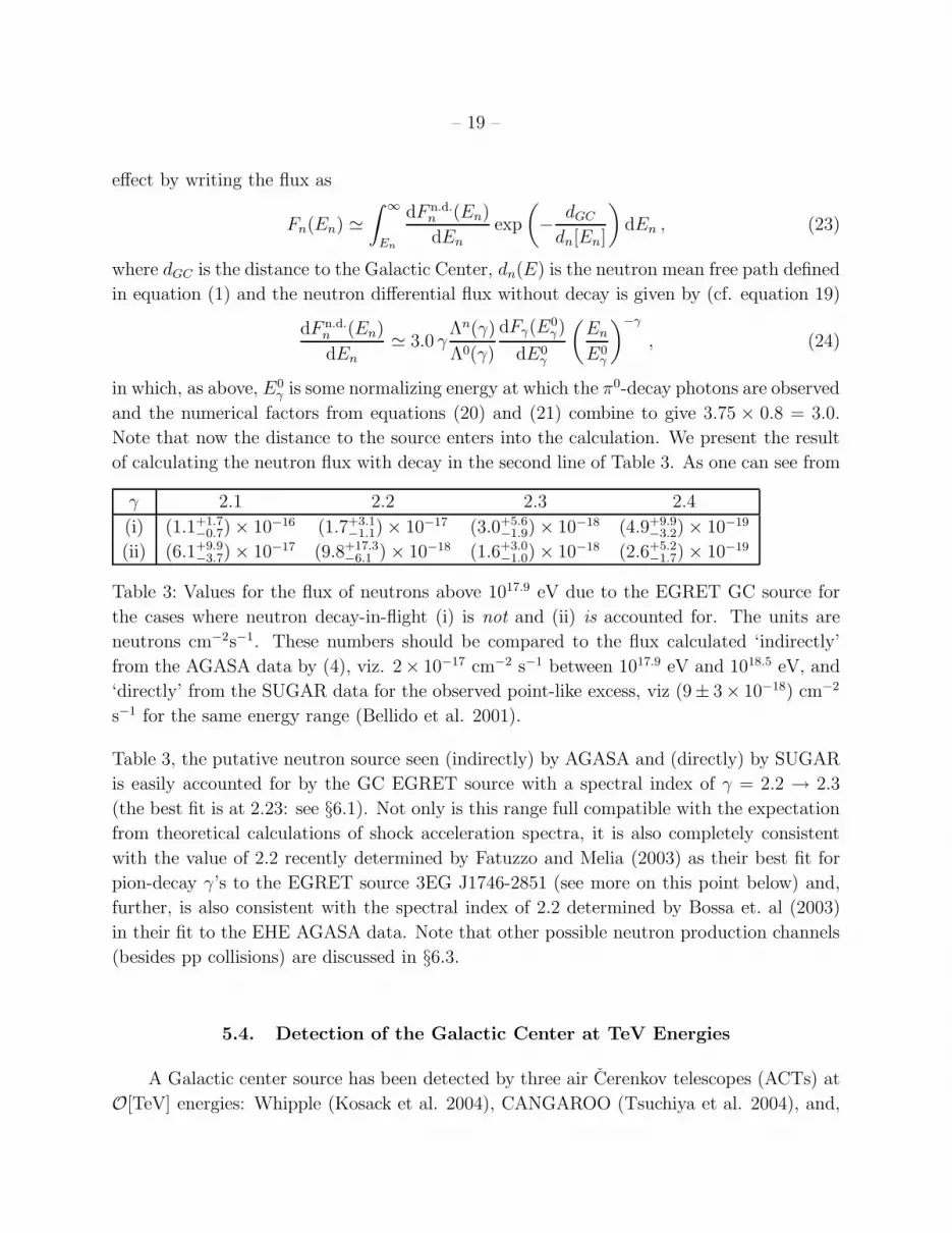
Note that now the distance to the source enters into the calculation. We present the result

of calculating the neutron flux with decay in the second line of Table 3. As one can see from

γ 2.1 2.2 2.3 2.4

(i) (1.1+1.7−0.7) × 10−16 (1.7+3.1

−1.1) × 10−17 (3.0+5.6−1.9) × 10−18 (4.9+9.9

−3.2) × 10−19

(ii) (6.1+9.9−3.7) × 10−17 (9.8+17.3

−6.1 ) × 10−18 (1.6+3.0−1.0) × 10−18 (2.6+5.2

−1.7) × 10−19

Table 3: Values for the flux of neutrons above 1017.9 eV due to the EGRET GC source for

the cases where neutron decay-in-flight (i) is not and (ii) is accounted for. The units are

neutrons cm−2s−1. These numbers should be compared to the flux calculated ‘indirectly’

from the AGASA data by (4), viz. 2× 10−17 cm−2 s−1 between 1017.9 eV and 1018.5 eV, and

‘directly’ from the SUGAR data for the observed point-like excess, viz (9± 3× 10−18) cm−2

s−1 for the same energy range (Bellido et al. 2001).

Table 3, the putative neutron source seen (indirectly) by AGASA and (directly) by SUGAR

is easily accounted for by the GC EGRET source with a spectral index of γ = 2.2 → 2.3

(the best fit is at 2.23: see §6.1). Not only is this range full compatible with the expectation

from theoretical calculations of shock acceleration spectra, it is also completely consistent

with the value of 2.2 recently determined by Fatuzzo and Melia (2003) as their best fit for

pion-decay γ’s to the EGRET source 3EG J1746-2851 (see more on this point below) and,

further, is also consistent with the spectral index of 2.2 determined by Bossa et. al (2003)

in their fit to the EHE AGASA data. Note that other possible neutron production channels

(besides pp collisions) are discussed in §6.3.

5.4. Detection of the Galactic Center at TeV Energies

A Galactic center source has been detected by three air Cerenkov telescopes (ACTs) at

O[TeV] energies: Whipple (Kosack et al. 2004), CANGAROO (Tsuchiya et al. 2004), and,

– 20 –

most recently and significantly, HESS (Aharonian et al. 2004). In addition, the Hegra ACT

instrument has put a (weak) upper limit on GC emission at 4.5 GeV (Aharonian et al. 2002)

and the Milagro water Cerenkov extensive air-shower array has released a preliminary finding

of a detection at similar energies from the ‘inner Galaxy’ (defined as l ∈ {20◦, 100◦} and

|b| < 5◦: Fleysher (2002)). Here we address only the Whipple, CANGAROO, and HESS

results in any detail, though note that all the observations mentioned above lend crucial

support to the notion that acceleration of particles to very high energies is taking place at

the GC.

Even restricting ourselves to consideration of results from these three instruments, we

find the situation somewhat confused regarding the GC. In fact, it was clear, even before

the arrival of the recent, remarkable data from the HESS instrument, that the Whipple and

CANGAROO GC observations were in conflict: Whipple has detected (in data collected

over a total of 26 hours from 1995 to 2003), at (conservatively) the 3.7 σ level, a flux of

photons from the GC direction of 1.6 ± 0.5 stat ± 0.3 sys × 10−12 cm−2 s−1 above 2.8 TeV

(Kosack et al. 2004) which is 40% of the Crab flux above this same energy. (In regards to

the errors on the measuremnt, note that there is a 20% uncertainty, too, in the callibration of

the 2.8 TeV energy threshold). This is to be contrasted with GC data which were collected in

2001 and 2002 by the CANGAROO-II ACT. From these data the CANGAROO collaboration

has been able to generate a spectrum for the GC source in six energy bins. From this

spectrum can be extracted (Hooper et al. 2004) a flux of around 2 × 10−10 cm−2 s−1 above

250 GeV: this is at the level of 10% of the Crab (Tsuchiya et al. 2004). The CANGAROO

Collaboration also determine an extremely steep spectrum for their GC source with a fitted

spectral index of 4.6 ± 0.5.

The fluxes of the Whipple and CANGAROO sources (relative to the Crab) are, then,

quite different and a natural reading of the situation is that the instruments are in conflict

(see Hooper et al. (2004) for further discussion on this point). Note that any variability of

the GC source at these energies is now constrained to be small (Kosack et al. 2004) so that,

though the two instruments in question collected their GC data over periods largely non-

coincident with each other, there is little leeway for explaining the difference between the

two instruments by positing that they happened to observe the source at different activity

levels. Also note that the fields-of-view of the two instruments are similar and that their

respective GC sources are at similar positions and of similar extent 5.

Adding very significantly to our knowledge of the GC at ∼ TeV energies, the High En-

ergy Stereoscopic System (HESS) Collaboration (Hinton 2004), which employs four imaging

5Steve Fegan, private communication.

– 21 –

atmospheric Cerenkov telescopes, has recently released TeV-range, GC data unprecedented

in its detail. This group has detected a signal in observations conducted over two epochs

(June/July 2003 and July/August 2003) with a 6.1 σ excess evident in the former and a 9.2

σ excess in the latter (Aharonian et al. 2004). The data from the larger, July/August 2003

data set (which we shall use in our analysis) can be fitted by a power law with, from the

collaboration’s own determination (Aharonian et al. 2004), a spectral index 2.21 ± 0.09 and

normalization (2.50 ± 0.21) × 10−8 m−2 s−1 TeV−1 with a total flux above the instrument’s

165 GeV threshold of (1.82± 0.22)× 10−7 m−2 s−1 (there is also a 15-20% error from energy

resolution uncertainty). Data from the June/July 2003 run are consistent within errors with

the July/August 2003 data.

The HESS flux determination is equivalent to 5% of that from the Crab above the 165

GeV threshold. It is in conflict with the results from Whipple (see figures 1 and 2), the

latter’s flux determination being a factor of three above that implied by the HESS spectrum

(Aharonian et al. 2004). It is also in striking conflict with the CANGAROO data: the HESS

spectral index determination is clearly at variance with the very steep spectrum found by

CANGAROO (see figure 4 of Aharonian (2004) for a clear illustration of this fact). Again,

one might interpret these discrepancies as evidence for significant source variation between

the the instruments’ different observing periods (i.e., over timescales of ∼ year) but the multi-

month HESS data no more indicate source variability within the observing period than the

previous observations (Aharonian et al. 2004).

Intriguingly, the HESS data are also difficult to reconcile with the EGRET GC data

(again, see figures 1 and 2 and also see the inset of figure 4 of Aharonian(2004)) – if one

assumes a single source. We shall have more to say about this issue below. For the moment,

however, we must clearly decide upon which of the TeV data sets we should base our analysis.

Certainly one telling point against the CANGAROO data, as noted above, is the unusually

steep, GC source spectrum. Although we do not pretend to any in-depth knowledge of the

workings of the CANGAROO analysis, we do note that observations of instrinsically bright

regions like the GC are, generically, affected by the problem that at lower energies putative

events can be ‘bumped over’ a detector’s threshold by noise, whereas at higher energies

such a mechanism would not be expected to be working6. A source spectrum, then, might

6One way around this potential problem is to employ a ‘padding’ procedure in which artificial noise is

fed into the data to account for the systematic brightness differences between on-source and background

observations. This is at the cost of reducing the signal-to-noise ratio and, therefore, raising the threshold

for observations but without such a procedure the artifical steepening of a power law is difficult to avoid.

Now, the VERITAS Collaboration, in its analysis of the Whipple data from sources located in bright regions

employs exactly the padding procedure described immediately above (Steve Fegan, private communication).

– 22 –

be made to seem steeper than in actuality by this preferential recording of lower energy

events. Furthermore, though the HESS and Whipple data are somewhat at variance, they

are certainly less in conflict than either result is with CANGAROO (again, see figure 4 of

Aharonian (2004)), so they support each other in a qualified sense. For these reason we focus

on the HESS and Whipple results and, then noting both the greater detail and statistical

weight in the former, we finally are drawn to the conclusion that we should leave only the

HESS data in our analysis.

6. Fitting to All Data

We will now attempt to derive a best fit to the following data: the EGRET γ-ray

differential flux at ∼ GeV energies, the HESS ∼ TeV γ-ray flux and the EHE (∼ 1018 eV)

cosmic ray anisotropy data (assumed due to neutrons). Such a fitting procedure makes sense

in principle because, as shown above, the neutron and photon fluxes are governed by power

laws with the same spectral index (as both these species arise from the interactions of the

same parent spectrum of accelerated protons) and at any energy we can relate the flux or

differential flux of neutrons and photons.

Our procedure is to define a χ2 function which depends on the differences between

fitted and observed fluxes or diffential fluxes, weighted by the experimental error in each

flux measurement and also allowing for the systematic uncertainty in the energy calibration

of the various instruments. The free parameters in our analysis are the spectral index, γ,

and the normalization of the γ-ray differential flux. We describe our procedure at greater

length in an appendix.

Employing this procedure, one quickly learns that the hypothesis that the totality of

γ-ray and cosmic ray data can be explained as arising from the interactions of a single, par-

ent population of shock-accelerated protons is not supported by the data: the fit procedure

produces a χ2 of 78.55 with a reduced χ2 of 6.54 for the (14 - 2) degrees of freedom (dof)

which is a very bad fit. There are a number of caveats to this bald assertion, however, which

we shall explore in somewhat greater detail below. These are, firstly, that it assumes that the

detected radiation – in its various energy regimes – is all equally unaffected in its propaga-

tion. A process which, say, attenuated γ-rays at TeV energies but not at GeV energies might

be operating but this is not accounted for in the fitting procedure. Secondly, the fits assumes

that there is, effectively, only a single source. The GC is a highly energetic and dense region;

But, to the best of our knowledge, the CANGAROO collaboration does not use this procedure. For this

reason we believe that the slope of the CANGAROO data on the GC source are questionable.

– 23 –

there could, in reality, then, be a number of effective sources or acceleration/interaction re-

gions (characterized by different magnetic field strengths, different shock compression ratios,

different shock/magnetic field geometries, different ambient particle densities, etc) there.

Thirdly, the fit procedure assumes that the detected particles/radiation all originate in the

same pp collision process. If, say, another process were operating at high energies to supply

some significant fraction of the observed neutrons, then accounting for this process might

allow for a better fit to the totality of data (that said, the EGRET and HESS data are still

difficult to reconcile). We now explore these various points in greater detail.

6.1. A Single Source: Attenuation of TeV Photons?

As should be expected from §5.3, if one performs a fit to only the EGRET+EHECR

data (‘EHECR’ denotes extremely high energy cosmic ray’: it is implicit in our analysis,

of course, that these data are explained as arising from neutron primaries), neglecting the

HESS data, one finds a very good fit: the total χ2 is 0.33 for (4 - 2) degrees of freedom for

a very plausible spectral index of 2.23. We remind the reader that this value is perfectly

consistent with that determined by Fatuzzo and Melia (2003) for the EGRET source 3EG

J1746-2851 and by Bossa, Mollerach, and Roulet (2003) for the EHE CR source seen by

AGASA (both these reference quote a figure of 2.2) and is, moreover, perfectly consonant

with the expectation from theory for acceleration at strong shocks. Further, the fitting points

are around eight orders of magnitude apart so it is, indeed, remarkable that the fit obtained

between such widely-separated data points should require a spectral index so close to the

expectation from shock acceleration theory and previous observations in more limited energy

regimes (see the upper line in figure 1).

The one problem with this scenario is the significant (by a factor of ∼20) overprediction

of TeV γ-rays (again, see figure 1). We note that there is no question but that our fit to

the EGRET+EHECR data does predict a TeV source which is inside the field of view of

HESS’s GC observations (and Whipple’s for that matter) and should have been seen by

this instrument. The simplest possibility to resolve the discrepancy, which we respectfully

submit, is that the normalization of HESS GC data is simply off by a large number. In

support of this, note that the other remarkable aspect of figure 1 is that the lower line –

which is a fit to the July/August 2003 HESS data alone – so closely parallels the upper: it has

a best-fit spectral index of 2.227. It does seem rather unlikely, however, that a normalization

7This spectral index has been independently re-derived by us: the HESS group find a spectral index

of 2.21 ± 0.09 with a normalization of 2.510−8 m−2 s−1 TeV−1 at 1 TeV. We perfectly agree with this

– 24 –

error could really be as large as we require it and (given also that even the larger Whipple

flux determination is still deficient with respect to our expectation from the single source

model) we are compelled to seek astrophysical explanations of the data considering them to

be fundamentally sound.

One possibility, presaged above, is that some process is acting to attenuate or downgrade

the energies of the ∼ TeV photons after they have been generated, i.e., in their propagation

from interaction point to us. In this regard, probably the most attractive mechanism is

pair-production on the optical-NIR background near the source. Certainly something like

this process is known to operate in the “self-absorption” of TeV γ-rays from some X-ray

binary systems by the thermal photons emitted by those systems’ own accretion disks (see

Moskalenko (1995) for a review). Pair production has an effective threshold which means

that it does not significantly attenuate γ-rays with energies below a threshold, Ethresh(pair)γ ,

given roughly by

Ethresh(pair)γ ∼ 1

(

Ebckgnd

0.5 eV

)−1

TeV , (25)

where Ebckgnd is the typical energy of the (relevant) background photon population. With

NIR-optical background light, then, the GC GeV signal would remain unattenuated as de-

sired. From equation (25) we require a background of ∼ 1.5 eV (i.e., NIR-optical) photons

to attenuate the HESS signal right down to the lowest datum at around 300 GeV. Further

considerations are the following:

1. Attenuation of the signal by ∼ 1/20 of the expectation (given the fit to the other data)

implies an optical depth of ln(20) ∼ 3

2. The peak cross-section for pair production is roughly 10−25 cm2, so we require a column

density of photons of around 3/10−25 cm2 = 3 × 1025 cm2 to attenuate the photons.

Over the entire 8.5 kpc to the GC this would require an average optical-NIR photon

number density of ∼ 1000 cm3. This is orders of magnitude larger than what is found

in the Galactic plane, so we shall concentrate on the idea that most attenuation will

happen very close to the GC source.

3. Given the similarities in the slopes of the fitted power laws shown in figure 1, the

attenuation/degradation should be energy independent over the observed TeV data

points. At the heuristic level, at least, pair-production can achieve something like

this (though this is somewhat dependent on the distribution of the target photon

population) once one accounts for the possibility that the daughter electron-positron

normalization to the limit of the significant figures quoted.

– 25 –

pairs go on to produce further, high energy γ-rays by inverse Compton scattering of

light in the background radiation field, thereby initiating a cascading process which

redistributes the photon energy8.

4. The main remaining question now is simply whether we can plausibly get a sufficient

column density of NIR-optical photons near a candidate GC source to effect the atten-

uation/degradation. For reasons that are explained in §8 the two objects we consider

plausible sources for the EHE cosmic rays are the accretion disk associated with the

GC black hole itself, Sgr A∗ and a supernova remnant located very close to the GC

called Sgr A East. We consider the photon environments in the immediate vicinity of

each of these before briefly considering the general, GC photon number density (i.e,

within ∼ 10 pc of the center).

(a) Sgr A∗: Genzel et al. (2003) find that the “local background subtracted” lumi-

nosity of Sgr A∗ in the NIR is ∼ 3.8 × 1034 erg.s−1. This means – assuming a

point source – a column density along a radial direction starting at r0 is given by

2.7×1034(r0/cm)−1cm2. Setting this equal to the required column density (3×1025

cm2) and inverting we find r0 ∼ 109 cm. But this is inside the Schwarzschild radius

of the central black hole (∼ 8 × 1011 cm) and, therefore, an unphysical require-

ment. The NIR light field due to the Sgr A∗ accretion disk, in other words, cannot

attenuate the TeV γ-rays to the extent we require. We note in passing that pos-

tulating a source location very close to the central black hole would present many

observational difficulties. These are summarised in §8.1

(b) Sgr A East: From fig 3 of Melia et al. (1998) the extrapolated synchrotron

flux at ∼ 1 eV for this object is 0.3 MeV cm−2 s−1 MeV−1. This translates

to a rough (number) luminosity of 2.6 × 1045 photons s−1, which is an order of

magnitude smaller than that for Sgr A* which means an analogous r0 many orders

of magnitude too small given the ∼ pc scales of the Sgr A East shock(s).

(c) General background: On the other hand, the actual quantity of interest is not

the background-subtracted luminosity nor the luminosity due to any particular

object. Rather, it is the total number density of suitable photon targets in the

GC environment. This we can estimate from the following consideration: Wolfire,

8In this regard, consider figures 6a and 6b of Carraminana (1992), which show the results of detailed

modeling of the “self-attenuation” of TeV γ-rays from two X-ray binary systems due to interactions with

thermal NIR and optical photons emitted by those systems’ own accretion disks. It can be seen in these

figures that the resultant (down-shifted) spectrum parallels the unmodified spectrum for up to an order of

magnitude in energy.

– 26 –

Tielens and Hollenbach (1990) find that the GC circumnuclear disk requires an

ionizing UV photon flux of 100-1000 erg cm−2 s−1. Taking the upper figure and

assuming the same energy density in NIR photons9 one finds (at ∼1 eV) a photon

number density of 2.1×104 cm−3. Again, given the specified column density, this

number density requires a length scale of 1.5× 1021 cm ∼ 500 pc to get sufficient

attenuation. This would seem to be excessive.

We reluctantly conclude, then, that around neither of the plausible, GC sources of the

EHE cosmic rays, nor in the general GC environment, does one find a large enough NIR-

optical photon number density (over sufficient scales) for our puposes: the optical depth to

pair production experienced by the TeV γ-rays in their propagation out of the GC environ-

ment is too small for us to explain the totality of data with a single source. We now consider,

therefore, the idea that two effective sources are contributing to the totality of data with

one source explaining the EGRET results and another (hopefully) able to account for both

the HESS and EHE cosmic ray observations. In this scenario we do not have a compelling

explanation for the closely parallel nature of the two fitted lines in figure 1 aside from the

general expectation from shock acceleration theory that the spectral index be close to 2.0 in

a strong shock.

6.2. Two Effective Sources?

In introducing the idea that there may be two effective 10 sources we note that this is

not an entirely unnatural reading of the situation. There are two pieces of evidence we bring

in here:

1. It has actually been determined by Hooper and Dingus (2002) in their re-analysis of

select data from the the 3EG catalog (Hartman et al. 1999) that the GC is excluded

at the 99.9 % confidence limit as the true position of the source 3EG J1746-2851 (this

determination is at variance with the findings made in the Hartman et al. (1999)

paper). Hooper and Dingus found the EGRET source to be fairly well localised to

9A re-processed IR photon background of similar energy density to the 30 000 K UV background is, in

fact, expected, but this would realistically peak at around 100 K ∼ 2.3× 10−2 eV: see §6.3.1. Given that, in

any case, we do not find any positive effect from the re-processed IR photons this detail need not concern

us.

10We emphasise ‘effective’ here because two or more apparent sources might in fact orginate from a

background population of protons accelerated in different regions of a single, extended object.

– 27 –

a position 0.21◦ south west of the GC (i.e., ∼ 5 pc at this distance). In contrast,

the HESS GC source was found to lie with 95% confidence within 0.05◦ of the GC

(Aharonian et al. 2004).

2. Both modeling and observation of SNRs over many years has consistently shown that

those examples with high flux tend to have a lower energy cutoff than those whose

spectrum extends to higher energies. This is generally attributed to the fact that

physical conditions that sponsor efficient acceleration also lead to efficient cooling at

higher energy. In general, then, the flux level and energy cutoff tend to go in opposite

directions (see, e.g., Baring (1999)).

On the quantitative side, the first item we must now check is whether a good fit is

possible to the combined HESS+EHECR data which, in this scenario, are supposed to be

explained by a single source (we call this assumed high-energy source the ‘HE source’). We

find this, indeed, to be the case: such a fit produces a χ2 value of 4.6 and a reduced χ2 of

0.51 for the (11 - 2) dof. The best fit spectral index is very hard: 1.97. If we constrain the

spectral to be 2.0 and fit only to the normalization we obtain a χ2 of 5.0 and a reduced χ2

of 0.50 for (11 - 1) dof (see figure 2).

The second issue we must confront is whether the other source (which we label the ‘LE

source’)– associated with the signal seen by EGRET – in any way interferes with the TeV

observations which are ascribed to the HE source. In particular, we must determine whether

the LE source is “overtaken” by the HE source at or below HESS energies as we require

(in order that ∼ TeV γ-rays not be overproduced). This might happen in either (or in an

effective combination of) two ways: (i) if the spectral slope of the LE source is sufficiently

steeper than the HE source and/or (ii) if the LE source cuts out below TeV energies (the

requirement that this source not produce a relatively significant flux of 300 GeV and above

γ-rays would be guaranteed if the parent protons cut out at or below ∼ TeV).

In regard to (i) and (ii) immediately above, we note firstly that (i) appears not to be the

case: we have tried two approaches here and both overpredict the differential γ-ray fluxes

at ∼ TeV by at least an order of magnitude. In the first approach we fit only to the three

(highest energy) EGRET data points for 3EG J1746-2851 with variable normalization and

spectral index. This naive approach produces a very steep spectral index of 2.6. In the

second approach we fit only to normalization fixing the spectral index to 2.4 which is at

the upper limit of the spectral index range for the parent proton spectrum as determined

by Fatuzzo and Melia (2003) in their fit to the totality of the EGRET data (i.e., all 9 data

points).

We should consider, then, whether (ii) could describe the situation.

– 28 –

The interesting question now is, therefore, how we arrange for the difference of something

like seven orders of magnitude between the maximum energies attained in the LE and HE

GC sources. Certainly variation in ambient particle densities and magnetic field strengths

will go some way towards explaining the difference, but it is doubtful that the combination

of these two could give a difference of 107. Another tenable hypothesis is that the LE source

– which in this scenario would be entirely independent of the HE source – has an age-limited

maximum energy. Another scenario would posit that the lion’s share of the difference may

be attributed to differences in shock geometries. In particular, one could postulate that the

HE source realize a perpendicular shock configuration and that the LE source be described

by a parallel configuration. This difference would be expected to contribute to at least two

orders of magnitude variation in maximum acceleration energies (all other considerations

aside): see §7, in particular, equations (38) and (39) below. Note that we would also expect

different shock compression ratios in the different effective sources so the generic expectation

would be for differing spectral indices.

6.3. Other Neutron Production Channels

There are two other channels which might reasonably contribute to EHE neutron pro-

duction at the GC, viz. p-γ and heavy ion dissociation. Both of these operate, effectively,

without producing a concomitant GeV or TeV γ-ray signal. This has the implication that

our calculation of EHE neutron production (normalized to this γ-ray signal) is, all other

things being equal, a strict under-estimate.

6.3.1. pγ interactions

We have performed detailed calculations of the pγ process within the ∆(1232) resonance

approximation (Stecker 1979; Mucke et al. 1999; Dermer 2002). In this context, the relevant

neutron production channel is through the first ∆ resonance at 1232 GeV,

pγ → ∆ → nπ+ , (26)

with a cross-section of about 6 × 10−28 cm2 (Hagiwara and al. 2002). Here the branching

ratios of the ∆(1232) lead to proton to neutron production in the well-defined ratio of 2:1 and

its decay kinematics predict a nucleon elasticity of 0.8 (Mucke et al. 1999). The interaction

can take place if the energy of the ambient photon in the p rest frame, Ethresh(pion)γ(p) , satisfies

Ethresh(pion)γ(p) ≥

m2∆ − m2

p

2mp

≃ 340 MeV . (27)

– 29 –

This means that the relevant target photon population in the GC context is supplied by the

intense flux of IR photons from the circumnuclear disk. This is a powerful source (≃ 107 L⊙)

of re-processed mid- to far-infrared continuum emission with a dust temperature of ≃ 100

K (Telesco 1996). Given this temperature, we find that the pγ process does not contribute

significantly for neutron production until proton energies of ≥ 6.9 × 1018 eV are reached,

or, given the elasticity, does not contribute significantly to neutrons with energies below

∼ 5.5 × 1018 eV. (The fact that this reaction does not ‘kick-in’ until such high energies

explains why it can not be directly normalized to the GeV γ-ray signal: despite the fact

that the decay of neutral pions from the other branch of the ∆ decay will certainly produce

photons, these will all be directly produced in the EHE regime.) This fact – our detailed

modeling shows – means that the pγ process produces a EHE neutron flux in the relevant

energy range, at most, O[1%] of that due to pp and may, therefore, be ignored.

Note that we have performed the calculations in this section assuming that the inter-

action region is at O[pc] scales from the GC (appropriate, e.g., to the closer-in parts of the

Sgr A East shell). We explain in §8.1 why it is unlikely that the interaction region be very

much closer to the GC than this

6.3.2. Heavy Ion Dissociation

A calculation of neutron production from dissociation of heavy ions (through interactions

with either ambient protons or light) is beyond the scope of this paper (Tkaczyk 1994). Such

interactions, moreover, do not lead directly to photon production at any energy and we can

not, therefore, normalize the rate of this process to the EGRET γ-ray data directly. Still,

that this mechanism might be operating we find entirely plausible especially given the fact

that heavy ions make up a non-negligible fraction of the detected cosmic ray population.

7. Limiting Energies

As remarked above, the flux figures listed in Table 3 implicitly assume that the power-

law description of the parent protons which (indirectly) generate the photons observed at

∼ 5 × 109 eV continues to hold up to much higher energies, 1018 eV and above. It also

assumes that the distribution of daughter neutrons continues to be set by the scaling relation

described in equation (16). This latter point we discuss in detail in an appendix. In brief,

– 30 –

we expect that the scaling relation will be correct to within a factor of two11, which, given

other uncertainties in the calculation, does not introduce a significant extra uncertainty in

our neutron flux calculations. Certainly, however, we need to devote considerable attention

to the former point regarding the maximum energies to which any particular known source

at the GC might accelerate protons. We shall see that considerations surrounding limiting

energy actually mean that we can – with some confidence – identify which of the potential

sources at the GC is responsible both for the EGRET-observed signal and the neutron signal.

In determing the limiting energy, Emaxp , two broad considerations play a part, viz (i) the

intrinsic limits to Emaxp given the macroscopic properties of the shock at the source doing

the acceleration (magnetic field strength, shock size, geometry, and age, etc) and (ii) limits

to Ep from heating-cooling balance which we label scattering limits.

We discuss both (i) and (ii) at greater length below.

7.1. Perpendicular Shock Acceleration

7.1.1. Transport

The whole of diffusive shock acceleration theory can be obtained from the Parker equa-

tion, the fundamental transport equation for the charged particle distribution function,

f(~r, t, p), in a background, collisionless hydromagnetic field (Parker 1965):

∂f

∂t=

∂

∂xi

[

κij∂f

∂xj

]

− Ui∂f

∂xi

+1

3

∂Ui

∂xi

∂f

∂ ln(p)+ Q(xi, t, p), (28)

where κij is the diffusion tensor and Q(xi, t, p) is the local source strength. This equa-

tion parametrizes the effects of diffusion, convection, and acceleration/deceleration by an

electric field on the charged particle distribution. The equation assumes that the diffusion

approximation holds good, i.e., that particles are scattered often enough by magnetic field

irregularities that the particle distribution is nearly isotropic. The Parker equation also re-

quires that the ratio of the shock speed, U = |U|, to the particle speed, w is small: U/w ≪ 1.

In this picture, particle acceleration is caused by two factors (Jokipii 1982, 1987):

1. the large relative motion between the (magnetic) scattering centers (i) causing the

diffusion in front of the shock and (ii) behind the shock

11Paolo Lipari, private communication, 2003.

– 31 –

2. (if the magnetic field has a component normal to the direction of propagation of the

shock) drift along the shock front.

Despite the potential importance of the second factor listed above, many discussions neglect

magnetic field changes and the resulting particle drifts, effectively restricting consideration

to quasi-parallel shocks.

From observation, it is known that the Galactic cosmic ray flux is quasi-isotropic to

high energy. This indicates that the Parker equation should hold as a valid description

of cosmic ray acceleration. The scattering of a charged particle depends most strongly

on the amplitude of magnetic turbulence on scales similar to that particle’s gyroradius.

This consideration justifies the ‘quasi-linear’ approximation in which the scattering rate is

taken to be proportional to the fluctuation spectrum of the magnetic field at a wavenumber

approximately equal to the inverse of the gyroradius.

7.1.2. Acceleration

Charged particle acceleration in the collisionless plasmas of space is through the action

of ambient electric fields, E. Because the relevant plasma processes are hydromagnetic (i.e.,

because we expect the charges to respond to changes in the electromagnetic field on a time

scale much shorter than the flow time, so that the Lorentz force in the plasma frame is

effectively zero) the electric field satisfies

E = −U × B. (29)

Note that though E does not appear explicitly in the Parker equation, it is implicitly con-

tained in U. We can arrive at a completely general description of diffusive shock acceleration

(i.e., applying equally well to parallel and perpendicular shocks and everything in between)

by putting a step-function U into the Parker equation.

In the strong shock limit, r, the ratio between the upstream and downstream flow

velocities satisfies

r =U1

U2

→ 4 (30)

(note that a subsript of 1 indicates a quantity measured upstream or in front of the shock,

whereas a subscript 2 indicates a quantity downstream or behind the shock). In this case,

it can be shown that the steady-state solution of the Parker equation indicates that the

momentum dependence of the particle distribution goes like f(p) ∝ p−4 corresponding to an

energy spectrum p2f ∝ p−2. This describes the universal power law (in either momentum or

– 32 –

energy) of spectral index close to 2.0 expected at strong shocks, whatever the particulars of

shock speed, diffusion coefficients, etc.

7.1.3. Acceleration Rate

In contrast to the spectral index, the high energy cut-off of the accelerated particles is

sensitive to the particulars of the shock. This maximum energy is largely determined by the

time available to accelerate the particles and the rate of energy gain. These, in turn, are

controlled by the finite lifetime of the shock itself, the escape of particles from the shock

region, and the rate at which particles scatter back and forth across the shock (collision and

synchrotron losses are also important, but these are dealt with below).

By solving the time-dependent Parker equation (and taking particles to be injected into

the shock at t0 with momentum p0), we can determine that the particle distribution is still

governed by the universal power law previously determined but now with a high momentum

cut-off, pc, which satisfiesdpc

dt≃ U2

shock

pc

4κxx, (31)

where κxx is the diffusion coefficient normal to the shock front. Either increasing the shock

speed, Ushock, or decreasing the diffusion coefficient, therefore, will produce a greater rate

of maximum momentum increase and, consequently, lead to faster particle acceleration in

general. Now, we can write the diffusion coefficient normal to the shock front as

κxx = κ‖ cos2(θB) + κ⊥ sin2(θB), (32)

where θB is the angle between the shock normal and the magnetic field vector. One can see

immediately, then, that, if the shock is quasi-perpendicular, κxx ≃ κ⊥, because κ⊥ is usually

smaller than κ‖, such a shock will tend to accelerate particles faster than a quasi-parallel

shock.

Let us consider the two limiting cases, quasi-parallel and quasi-perpendicular shocks, in

a little more detail.

7.1.4. Quasi-parallel Shocks

This is the more-commonly investigated case. From equation (31) we shall have that

1

pc

dpc

dt≃ U2

shock

4κ‖

=3U2

shock

4λ‖w, (33)

– 33 –

where λ‖ is the mean free path along the shock. Now, given that this quantity must be of

the order of or larger than the gyroradius of a particle at the limiting upper momentum,

rg(pc) ≡ rc, we find that1

pc

dpc

dt.

3U2shock

4rcw, (34)

which is the so-called Bohm limit on the acceleration rate. Many researchers have taken this

to represent a mechanism-independent limit on the acceleration rate and, hence, indirectly

on Emax. The logic implicit here is that in order to be turned about so that it re-crosses the

shock, a particle must be re-scattered each time it moves up- or downstream of the shock.

The highest energy gain rate, by this logic, will then occur for the smallest scattering mean

free path, which, in turn, cannot be smaller than the gyroradius.

7.1.5. Quasi-perpendicular Shocks

The reasoning presented above does not have universal validity, however: if the magnetic

field has a component perpendicular to the shock propagation direction and if (as is usually

the case as mentioned above) κ‖ > κ⊥ (so that the particle is less constrained in motion

along the shock than in motion away from it), the gyromotion of a charged particle can

carry it across the shock many times between each scattering. This can mean a much larger

Emax than for the parallel case.

To see this quantitatively, note that the kinetic theory (i.e., billiard ball scattering)

value for the ratio between perpendicular and parallel diffusion coefficients is given by

κ⊥

κ‖

=1

1 +(

λ‖/rg

)2 , (35)

so that for a larger parallel mean free path, the perpendicular diffusion coefficient is reduced

and the acceleration is, therefore increased (to be contrasted with the parallel case for which

a smaller parallel mean free path means an increase in the acceleration rate).

It seems that if we want acceleration to very high energies we should simply dial up the

required λ‖. This quantity may not be increased without limit, however. There will, in fact,

be a maximum value for λ‖ which can be determined (interchangeably) by the logic that

(i) the diffusion approximation implicit in the Parker equation ceases to be valid if particles

do not scatter often enough to be isotropic at the shock or (ii) particles must scatter often

enough to diffuse upstream fast enough to stay ahead of the shock (Jokipii 1982; Jokipii 1987)

Either of these two conditions leads to the requirement that

Υ ≡ Ushockrg

κ⊥≪ 1, (36)

– 34 –

or, for simple scattering

Υ ≃ λ‖

rg

Ushock

w≪ 1, (37)

so that if Ushock/w ≪ 1 then we can have λ‖/rg ≫ 1 (while still maintaining Eq. 37), giving

us a significant enhancement over the Bohm acceleration rate.

7.1.6. Limiting Energies in Diffusive Shock Acceleration at Supernova Remnants

Postulating that the maximum energy to which a Supernova Remnant (SNR) shock

might accelerate particles, ESNRmax is given by (i) the Bohm value of the diffusion coefficient

and (ii) the modified Sedov solution for Ushock, Lagage et al. (1983) determined that

ESNRmax ∼ EL&C

max ≡ few × 1014 × ZeV (38)

for the distance and magnetic field scales typical for a Galactic SNR. Given that, as outlined

above, SNRs are expected to accelerate the bulk of the cosmic rays up to at least the knee at

∼ 5×1015 eV, equation (38) would seem to place a severe constraint on the mass composition

of the cosmic rays.

Following from the arguments presented above, however, Lagage and Cesarky’s result

will not apply to quasi-perpendicular shocks. The sort of (globally) spherical shock pro-

duced by a supernova, moreover, is quasi-perpendicular over much of its area, meaning that

κ⊥ is much more important that κ‖ over a substantial fraction of the SNR shock and the

acceleration rate can be much larger than the Bohm limit. This means EL&Cmax is actually

a significant underestimate of ESNRmax which, by putting Υ equal to its maximum value, viz.

∼ 0.3, in equation (37) we can determine to be

Emax(perp)Z ∼ 5 × 1016 × Z

(

B

20 µG

) (

Rshock

10 pc

)

eV (39)

for a particle or nucleus of charge Z (see Appendix C for a full derivation of the limiting en-

ergy). Note that in the equation above “perp” signifies that the maximum energy appertains

to acceleration in a perpendicular shock geometry (Jokipii 1982; Jokipii 1987). This energy

is amply large enough to accelerate cosmic rays beyond the knee but note that equation (39)

represents an in-principle limit: in general, cooling effects due to synchrotron radiation or

collisions between the accelerated protons (and ions) and ambient matter or light may more

tightly limit the maximum energy/momentum to which the high energy particle population

can be accelerated. Further, the time available for acceleration is, of course, bound by the

total age of the shock. We now discuss these additional constraints.

– 35 –

7.2. Cooling- and Age-Imposed Limits to Maximum Particle Energies

There will, in general, be a maximum proton energy Emaxp above which the combined

energy loss rate due to many processes – proton synchrotron emission, inverse Compton

scattering and hadronic collisions (with ambient nucleons and γ’s) – will exceed the rate of

energy gain due to shock acceleration.

In the GC environment, however, pp collisions are, by far, the dominant energy-loss

process (Markoff et al. 1997; Melia et al. 1998; Fatuzzo and Melia 2003). This is the

case becasue of the relatively lower density of target photons and the intrinsically smaller

cross-sections and inelasticities of pγ processes in comparison with pp collisions (this is to

be contrasted with the situation that generally pertains in AGN, where the photon density

can be significantly higher than in the GC).

This maximum energy, Emax(cool)p , attainable given that pp collisions are occuring, de-

pends on the functional form of the average collision inelasticity, where inelasticity denotes

the fractional energy loss in the collision (i.e., the energy of the leading baryon in units of

the energy of the incoming proton). The time scale for proton cooling via pp collisions, then,

is given by

tpp ≃1

np c σppKpp, (40)

where the proton-proton cross-section, σpp, and the fractional energy loss per pp collision or

inelasticity, Kpp, are both, in principle dependent on energy (see the appendix).

On the other hand, the proton (shock) acceleration time scale is given by (Begelman

1990)

taccp (Ep) =Ep

ηc2eB, (41)

where η is a dimensionless parameter, O[1], that depends on the details of the acceleration

mechanism.

We can determine Emaxp , then, by setting

tpp = taccp (Emaxp ) (42)

and inverting to find

Emax(cool)p =

cηeB

npσppKpp. (43)

Finally in regard to maximum energies, one must also check that the time-scale implied

by equation (41) for the maximum energy calculated using equation (43) does not exceed

– 36 –

the age, tage, of the pertinent astrophysical object or environment. If this is the case, the

maximum energy will be age limited, i.e.,

Emax(time)p = ηc2eBtage ≃ 2.4 × 1018

(

B

20 µG

) (

tage20 104 yr

)

eV . (44)

In general we shall have, then,

Emaxp = min{Emax(perp)

p , Emax(cool)p , Emax(time)

p }, (45)

where the maximum energies are given, respectively, by equations (39), (43), and (44).

8. Identifying the GC Neutron Source

8.1. Sgr A∗ as EHE GC Neutron Source

The question of the maximum energy to which protons might be accelerated at the

Sgr A∗ shock has been addressed at some length by Markoff et al. (1999) and here we

simply quote their results. As presaged above, these authors found that pp collisions are the

dominant energy loss process for relativistic protons: pγ processes are supressed relative to

the expectation from other galactic nuclei due to the very low luminosity of the GC and pe−

processes are also suppressed due to a dearth of extremely energetic electrons. Taking the

mass of the central black hole to be 2.61 ± 0.65 × 106 M⊙ (Eckart and Genzel 1997)12, the

shock to be located at 40 Schwarzschild radii, a (generously large) magnetic field of ≃ 300 G,

and, finally, an ambient proton density of ≃ 2 × 108 cm−3, Markoff et al. (1999) determine

that the maximum attainable Lorentz factor for relativitic protons is approximately 4× 108

which translates to Emaxp ≃ 4 × 1017 eV. This maximum energy, then, means that Sgr A∗ is

probably not the source of the putative EHE neutrons seen by AGASA and SUGAR (indeed,

even if the anisotropy is due to the direct interactions of the primary,accelerated protons, it

still cannot be the source).

Another factor supporting the view that Sgr A* cannot be the source of the observed EeV

neutron flux would be the inconsistency implied by the emissivity of secondary particles. The

ensuing particle cascade would produce a copious supply of energetic electrons and positrons

that, in the presence of the inferred ∼ 1 − 10 Gauss magnetic field (let alone the 300 G

12Note that a recent revision to the Galactic center black hole mass that determines it to be 4.1± 0.6 M⊙

(Ghez et al. 2003) does not substantially alter the conclusion of Markoff et al. (1999) regarding maximum

attainable energies for shocked protons.

– 37 –

field we used for the estimate above) for this source, would greatly exceed Sgr A*’s observed

radio flux. This problem is alleviated if instead the secondary particles gyrate in the much

weaker field associated with a typical supernova shell. Finally, Kosack et al. (2004) make the

point that the lack of variability seen in their ∼ TeV γ-data for the GC source tells against

the identification of this source with a compact point source such as Sgr A* (no evidence

for variability is seen in the EGRET data for 3EG J1746-2851 either: Mayer-Hasselwander

et al. 1998).

8.2. Sgr A East as EHE GC Neutron Source

8.2.1. Introduction to Sgr A East

Sgr A East is a mixed-morphology, O[104]-year-old supernova remnant (SNR) located

within several parsecs of the Galactic Center (GC) (see Melia and Falcke 2001). It appears to

be of the class of SNRs which have been observed and detected at 1720 MHz (the transition

energy of OH maser emission), such emission being a signature of shocks produced at the

interface between supersonic outflow and the dense molecular cloud environments with which

these SNRs are known to be interacting. There is, further, good evidence (see below) that

Sgr A East may be associated with the EGRET source 3EG J1746-2851 introduced in §4.

It should be remarked, however, that if this putative association is real, Sgr A East has a

γ-ray luminosity (∼ 2 × 1037 erg s−1) almost two orders of magnitude greater than that of

the other EGRET-detected SNRs, something which clearly demands explanation.

In fact, in a self-consistent scenario explored elsewhere (Melia et al. 1998; Fatuzzo and

Melia 2003) the Sgr A East remnant has been shown to be capable of producing the observed

γ-ray luminosity once the unusually-high ambient particle density (& 103 cm−3) and strong

magnetic field (& 0.1 − 0.2 mG) at the GC are taken into account. Indeed, let us make

the natural assumption that there is a population of protons at Sgr A East accelerated by

the shocks associated with the supernova blast wave (and, therefore, governed by a power

law with spectral index ∼ 2). Then, from collisions between these high energy protons and

ambient ions, pions will be produced and these will, in turn, decay to produce γ’s. Now, the

high-energy γ-ray luminosity in this scenario is essentially dependent on the rate of collisions

between ambient ions and high energy protons, which is, in turn, dependent on the product

of the ambient ion density and the high energy proton density, nHn0. So, we can fit to

these two on the basis of the observed γ-ray spectrum. We also have, however, a handle on

nH from observations by ACIS on board the Chandra X-ray Observatory – Sgr A East is

expanding into an ionized gas halo with a density ∼ 103 cm−3 and interacting with a cloud

of density ∼ 105 cm−3. Further, the total energy in the accelerated proton population is

– 38 –

readily calculated from n0 and is, of course, constrained to be less than the total energy

released in the original explosion that gave birth to the Sgr A East shell.

These considerations result in fairly rigorous contraints on any attempted fit to obser-

vations of Sgr A East . But, with a proper treatment of pion production (in particular, the

energy dependence of the pion multiplicity), the entire broadband spectrum of the object

can be compellingly explained. This explanation essentially sees the super-100 MeV γ-ray

spectum as due to π0 decay, the sub-100 MeV γ-ray spectum explained by bremsstrahlung

emission (self-consistently with the assumed value for nH, namely 103 cm−3: see below)

and the VLA observations of Sgr A East at 6 and 20 cm explained by synchrotron emission

(though see below for a caveat regarding the radio spectrum). Note that in this scenario, it is

the secondary, charged leptons (ultimately resulting from collisions of the shock accelerated

protons with ambient ions) that are responsible for the bremsstrahlung and synchrotron emis-

sion, rather than directly accelerated leptons. Indeed, the population of this primary lepton

class can, in fact, be shown to be negligible in comparison with the secondaries, given that

each accelerated proton produces of order 20-30 charged leptons (Fatuzzo and Melia 2003).

In regard to Sgr A East’s radio spectrum, it should be noted that the synchrotron emis-

sion from the total population of secondary, charged leptons is not directly consistent with ra-

dio observations: the observed spectral index is ∼ 1, pointing to an underlying population of

non-thermal charged leptons with a power-law distribution of index ∼ 3 (Pedlar et al. 1989).

In contrast, from general considerations (whether the lepton population is directly acceler-

ated or born of the interactions of shock accelerated protons), we expect that the lepton

index be ∼ 2, leading to radio emission characterized by a spectral index ∼ 0.5. If, however,

one allows for the reasonable eventuality that high energy leptons diffuse out of the Sgr A

East region, the convolution of a diffusion loss factor with the initial lepton spectrum result-

ing from pion decay allows a very good fit to the radio spectrum (Fatuzzo and Melia 2003).

Alternatively, it might be that the high energy protons themselves are diffusing out of the

system thus also (indirectly) depleting the high-energy lepton spectrum. This scenario also

provides a credible, though less good, fit to the radio data. As will become clear, however,

the very fact that we do see a GC EHE cosmic-ray anisotropy argues against the latter

scenario.

The scenario presented above – which we label ‘HIGH’ – is to be contrasted with an al-

ternative picture (‘LOW’) explored earlier (Melia et al. 1998), in which a considerably lower

ambient particle density was employed (viz. ∼ 10 cm−3). Through the nHn0 dependence

of the γ-ray luminosity this then necessitated a large population of high energy protons,

in turn yielding an energy content of relatitivistic particles of ∼ 8 × 1050 erg. In contrast,

the particle energy calculated for the HIGH scenario is ∼ 1049 erg so clearly the view that

– 39 –

Sgr A East resulted from a standard supernova favors HIGH. Moreover, the recent Chandra

observations of Sgr A East alluded to above support the view that Sgr A East is, indeed,

the remnant of a single supernova with typical energetics.

8.2.2. Maximum Energy of Protons Accelerated by the Sgr A East Shock

Typically, the magnetic field strength in the interstellar medium scales as the square

root of the density. In the case of Sgr A East, it appears that most of the pp scatterings (and

essentially all of the bremsstrahlung and synchrotron emissivity) occur in the ∼ 103 cm−3

region, where the field strength is ∼ 0.2 mG. Thus, if the shock occurs in the ∼ 105 cm−3

molecular cloud colliding with the expanding shell, the field intensity within the particle

acceleration region may be as high as a few mG. However, a value greater than this seems

implausible.

With a field strength of 4 mG, the other inputs described above, and the application of

equation (39), one finds that particles in the Sgr A East shock can be accelerated, in principle,

to 1019Rshock/10 pc Z eV. This figure is not limited by cooling or age considerations: from

equation (43) we find that, given the assumed 3,000 cm−3 ambient proton density13, a lower

limit on the cooling-limited maximum energy is 2.7 η 1021 eV (this is a lower limit because

it has been derived assuming a pp cross-section of 150 mb, which, in fact, only pertains at

the very highest region of the pertinent energy range). Moreover, the time required by the

4 mG field to accelerate protons to this energy is around 2 500 years, comfortably inside

the O[104] year age of the remnant (the age-limited energy using equation (44) is around

η5 × 1020 eV for a 4 mG field and an age of 10 000 years).

Parenthetically, note from the above that heavier ions might be accelerated to energies

approaching 1020 at Sgr A East – potentially explaining most of the cosmic ray spectrum even

above the ankle. If this were the case, it would not imply an unambiguous anisotropy towards

the GC: even at 1019 eV modeling shows that a proton leaving the vicinity of the GC would

be scattered many times, on average, before it could reach us at Earth. This mechanism

would isotropise the GC signal even at these extreme energies, though they would probably

not completely wash it out. Such a scenario is not ruled out by current observations.

13As is the case at Sgr A∗, pp collisions are the dominant cooling mechanism for relativistic protons

accelerated at the Sgr A East shock (Melia et al. 1998; Fatuzzo and Melia 2003).

– 40 –

8.2.3. Sgr A East and the Two Source Model

We note finally that there being two effective sources required to explain the totality of

data fits naturally into the hypothesis that the Sgr A East shell accelerates all the protons

required to explain the various signals. The Sgr A East shell ranges in distance from very

close to the GC (within 1 pc) to up to ∼ 10 pc. It subtends, therefore, regions of widely

varying ambient particle density and also magnetic field strength and orientation so that

proton populations accelerated in it would be expected to display or experience varying

maximum energies, spectral indices and overall (energy) differential number densities and

interaction rates. Moreover, Hooper and Dingus’s (2002) determination that the EGRET

source can be localized to a region 0.21◦ (i.e., ∼ 5 pc) away from the actual GC (while the

HESS source is localized to within 1 pc of the GC) supports this basic idea: the lower energy

source is located in a region where ambient magnetic fields can be expected to be lower

and also, perhaps, where ambient particle densities be higher, whereas the higher energy

source is located in a region of larger magnetic field strength. We hypothesise also that

the acceleration in these regions be described by different shock/magnetic field geometries

(with the EGRET source describing a parallel shock-magnetic field configuration and the

HESS/cosmic ray source being described by the more efficiently-accelerating perpendicular

configuration). Further observations and modeling will be required to determine whether

this picture is tenable.

9. Conclusion

We have examined – and shown to be quantitatively successful – the idea that the Galac-

tic center EGRET source 3EG J1746-2851 is also responsible for the observed anisotropy

that is seen in cosmic rays towards the GC at an energy of around 1018 eV. We have, in par-

ticular, demonstrated that a power-law fit to the ∼ GeV EGRET data and the EHE cosmic

ray anisotropy data (taking the latter to be evidence for neutron primary particles) requires

a parent proton population with a spectral index of 2.23. This is in exact agreement with

previous determinations made (individually) for the spectral indices of the parent proton

population that is generating the EGRET-observed γ-rays and for the distribution of the

EHE cosmic ray signal. The determined spectral index is also in perfect agreement with

the expectation from shock acceleration theory. Our fitting procedure requires input from

the particle physics of charge-exchange in pp collisions. Our results imply the existence of a

population of shock-accelerated protons (and perhaps heavier ions) at the GC with energies

that range up to, at least, ∼ 1019 eV.

Unfortunately, however, this fit overpredicts the flux of γ-rays from the GC at ∼ TeV

– 41 –

energies given the existing data from a number of atmospheric Cerenkov telescopes (which

are, admittedly, somewhat at variance amongst themselves). We show that what we believe

to be the best and most recent data – that coming from the HESS instrument – is well fitted

by a power law with a spectral index of 2.22, i.e., very close to the power law fit to the

combined EGRET and EHE cosmic ray data. One explanation, then, of the deficiency of

the ∼ TeV data with respect to expectation is that the HESS instrument’s normalization

is wrong by a large (energy-independent) factor (∼ 20). Finding this somewhat unlikely,

however, we have sought astrophysical explanations of the totality of EGRET + HESS +

EHECR data, taking these all to be fundamentally sound. Pursuing the idea that all the

data might be explained as originating from the interactions of a single high energy proton

population, we searched for mechanisms that would (preferentially) attenuate the ∼ TeV

γ-rays. The most promising candidate in this direction, however, viz, pair production on an

assumed 1.5 eV light background, we have found is unlikely to be efficacious as the number

density of such photons in and around candidate GC sources or source regions is probably

too low.

Noting these facts, we sought for a model involving two effective sources. We showed

here that the hypothesis that the EGRET data are explained by one source and the HESS

+ EHECR data by another is perfectly tenable with, in particular, a good fit possible to the

combined HESS + EHECR data. This two source scenario – which has some plausibility

given the varying source position determinations made on the basis of observations conducted

in the various energy regimes – requires that the EGRET source probably be steeper than

– and certainly have a cut-off energy much lower than – the HESS + EHECR source.

This difference in maximum particle energies could be attributed to either completely

independent populations of high energy protons, accelerated in different astrophysical sources

with differing ages, magnetic field strengths, ambient particle densities, etc. Alternatively

– and more plausibly in our opinion – a population of high energy protons accelerated in

different regions (with differing magnetic field/shock geometries) of a single, extended object

might produce two (or more) effective sources.

We have shown that the Sgr A East supernova remnant (located near the GC) could

provide the environment in which the acceleration of the high energy protons we require could

plausibly be achieved. Further, we have shown that the ‘two-source’ model fits naturally with

the hypothesis that Sgr A East is the accelerated proton source: the Sgr A East shell ranges

in distance from very close to the GC (within 1 pc) to up to 10 pc distance. It subtends,

therefore, regions of widely varying ambient particle density and magnetic field strength

and orientation so that proton populations accelerated in it would be expected to display

or experience varying maximum energies, spectral indices and overall (energy) differential

– 42 –

number densities and interaction rates. On the other hand, it seems that the other plausible

GC source, namely the accretion disk around the GC black hole, Sgr A∗, is unlikely to

provide an environment in which acceleration of protons to the extreme energies required is

possible. Further, observations tell against a point-like source for both the GeV and TeV

regime γ-rays. Our results, then, provide tentative evidence for the first direct connection

between a particular, Galactic object (Sgr A East) and the acceleration of cosmic rays up to

energies near the ankle in the cosmic ray spectrum.

At all energies, we anticipate – with great interest – the results that shall be obtained

by the next generation of instruments. These instruments include the GLAST Large Area

Telescope (Thompson 2004) at ∼ GeV energies and VERITAS (Krennrich et al. 2004), at

∼ TeV energies, and, finally, the Pierre Auger Observatory (Camin 2004) for cosmic rays of

1018 eV and higher. The results from these instruments will either confirm or rule-out our

scenario.

10. Acknowledgments

RMC gratefully acknowledges useful communications from Paolo Lipari and enlightening

conversations with Matt Holman, Jasmina Lazendic, Avi Loeb, and Josh Winn. FM would

like to thank Steve Fegan and Trevor Weekes for very helpful correspondence. This research

was supported in part by NASA grant NAG5-9205 and NSF grant 0402502 at the University

of Arizona. RRV and FM are also partially supported by a joint Linkage-International grant

from the Australian Research Council. RRV thanks Paolo Lipari and Todor Stanev for

general discussions on cosmic rays and the observed anisotropies, and he thanks Paolo Lipari

and Maxim Khlopov for their kind hospitality at the Universita di Roma “La Sapienza”

where these discussions took place. MF is supported by the Hauck Foundation through

Xavier University.

11. Appendix: Neutron Production in UHE Hadronic Interactions

We discuss here the necessary, particle physics inputs to our calculation of neutron

production, viz. the total (inelastic) pp cross-section, the leading neutron multiplicity in pp

interactions and the leading neutron elasticity in pp. In summary of the below, all three of

these quantities might in principle exhibit a scaling-violating dependence on the center of

mass energy. The data on the EHE cross-section are fairly sound and do indicate exactly

such a dependence, albeit a weak one. We account for cross-section growth as set out in §5.2.

– 43 –

There is no data at EHE on neutron multiplicity or inelasticity and, indeed, even at moderate

energies the data are scant. Modeling, however, predicts little or no energy dependence in

these quantities (note that we are talking about the production of leading particles, not

secondaries). We take it, then, that the leading neutron multiplicity and elasticity do not

evolve from the values supplied by the low energy data.

11.1. Leading Neutrons from pp Collisions: General Remarks

By definition, leading baryons (proton, neutron, or hyperon) created in pp (or pA)

collisions are those particles that carry a large fraction of the incoming hadron’s momentum.

On the other hand, these particles, can be expected to have, in general, a low transverse

momentum (see Eq. 49 below), i.e., leading particle production is a soft process. The

transverse momentum transfer, moreover, can almost be taken to be unrelated to the energies

of the primaries (or, indeed, the secondaries) and is, instead, at an intuitive level at least,

related to the inverse of the ‘size’ of the interacting hadrons ∼ 1/fm (e.g., Perkins (1987)).

To calculate the leading neutron production rate in pp collisions with ‘beam’ protons

of lab energy & 5 × 1018 eV we need to know

1. What the total (inelastic) pp cross-section is at such an energy.

2. What proportion of pp interactions at such energies result in the production of leading

neutrons, i.e. the leading neutron multiplicity. We expect here a number less than

unity that we could equally well describe as the charge exchange probability (in pp

interactions).

3. What fraction of the incoming proton’s energy any leading neutron will typically have

(i.e., the quantity for the leading neutron that has traditionally been labeled the elas-

ticity by cosmic ray investigators).

We discuss the empirical inputs to each of these three in turn below, before we go on to

consider theory and modeling.

11.2. Hadronic Cross-sections at High Energies: Experiment

Unlike the cases presented by leading particle multiplicities and inelasticities, hadronic

cross-sections have been measured (almost) up to the highest center-of-mass energies we are

– 44 –

interested in (√

s ∼ 50 TeV), though it should be noted that at the highest energies the

pp cross-section is extracted – using Glauber theory (Glauber and Matthiae 1970) – from

cosmic-ray data on proton-‘air’ nucleus interactions (see, e.g., Block (3)). Moreover, between

∼ 1011 eV and 1013 eV the cross-section has not been directly measured. These two facts,

however, do not allow for any great uncertainty in the cross-section: clear of the various

resonances at a few GeV, the growth of the total pp cross-section becomes smooth and

slow in the measured region. Further, there is a strict bound, the Froissart-Martin bound

(Froissart 1961; Martin 1965), on the asymptotic behaviour of the total cross-section, viz.,

for s → ∞σtot ≤ C ln2 s. (46)

From parametrization of the growth of the total pp cross-section between collider energies

and UHE cosmic ray data, the Froissart bound may be saturated.

As noted in the body of the paper, we take the pp cross-section to be constant for beam

energies between about 1010 eV and 1012 eV which, from from fig. 39.12 of Hagiwara et al.

(2002) is quite reasonable. On the other hand, we do allow for the slow growth (Hagiwara

2002) of the cross-section between this energy regime and that relevant to the EHE neutron

production.

11.3. Leading Neutron Multiplicity in Proton-Proton Interactions:

Experiment

At the EeV energy regime we are interested in, there is no direct, empirical data on

leading neutron production. Indeed, there are, in general, great difficulties in obtaining

information on production of (even) charged leading particles from colliding beam devices

(let alone neutrons). This is because the combination of large longitudinal and relatively

low transverse momentum that, as mentioned above, characterizes leading particles means

that they are kinematically constrained to emerge from their creation region at small angles.

They will, therefore, be traveling down a collider’s beam pipe where there is little or no

detector acceptance. In fact, for pp → leading n, the most recent and highest energy data

were obtained in the mid 1970s at experiments conducted at up to√

s ∼ 63 GeV at the

ISR (Engler et al. 1975; Flauger and Monning 1976) — three orders of magnitude below

the energy regime we are interested in — and Fermilab (Dao et al. 1974). These data are

described to first order by Feynman scaling (Feynman 1969) which reflects the partonic

make-up of the colliding protons (see below). Also of relevance, data have been obtained for

leading neutron production in proton-heavy ion (pA) and heavy ion-heavy ion collisions (for

recent data see, e.g. Barish et al. 2002, Huang et al. 2002, Armstrong et al. 1999) and for

– 45 –

e+p collisions by the ZEUS Collaboration at Hera (Chekanov and al. 2002; Levman 2002b;

Levman 2002a).

In the astrophysics literature a wide range of values for the leading neutron multiplicity

has been employed from ∼ 0.1 (Contopoulos and Kazanas 1995) to ∼ 0.5 (Berezinskii &

Gazizov 1977) with values close to one quarter perhaps most generally being favored (e.g.,

Sikora (1989); Jones (1990); Drury (1994)). But, given that this preference seems a matter

of lore, one must really look to the data.

Unfortunately, here again the picture is not entirely clear. From fits to the ISR data

(Engler et al. 1975; Flauger and Monning 1976), obtained at CMS energies between around

16 and 63 GeV, various researchers have determined values for the leading neutron multi-

plicity, nn, between 0.25 and 0.40. Though we have not re-analysed the data ourselves, our

considered opinion is that a neutron multiplicity at the higher end of this range is actually

the best motivated. In support of this position, note that, for instance, though (from the ISR

data) Frichter (13) obtain nn = 0.27, they also find a value for the leading proton multiplic-

ity, np, of 0.62 which, together with the constraint that np + nn = 1 (where leading hyperon

production, as supported by the data, can be neglected approximately), is consistent with

a value for the leading neutron multiplicity at the higher end of the above range (and, of

course, the proton is generically easier to track than the neutron). Also note that from

the same data, Forti et al. (1990) find nn = .40. Further, from lower energy experiments

conducted at the 2m hydrogen bubble at the CERN proton synchrotron in the late 1970s,

Blobel et al. (1978) determine σn/(σp +σn) to be ∼ 0.38 and 0.35 at CMS energies of 12 and

24 GeV respectively (where σp and σn are, respectively, the total, inclusive cross-sections

for pp → ppX and pp → pnX). As we set out below, the more sophisticated theoretical

treatments also predict a leading neutron multiplicity closer to one half than one quarter.

In conclusion, therefore, we take it that the value of nn is 0.40 at ISR energies.

11.4. Leading Neutron Elasticity in Proton-Proton Interactions: Experiment

Again, there is a complete lack of direct, leading particle inelasticty measurements at

the EeV energy scales we are concerned with and we can only look to the ISR data. For the

Feynman x variable

xF ≡ p‖/pmax‖ ≃ 2p‖/

√s, (47)

which, at the energies of interest we can take to be indentical to the inelasticity, Frichter

(13) find from the ISR data average values for protons and neutrons of 〈xF p〉 = 0.44 and

〈xF n〉 = 0.26. The fact that the data indicate that leading neutrons be softer than leading

protons is consistent with the expectation from theory: see below.

– 46 –

11.5. Theory at Low Energies and the Interpretation of the ISR Data

If Feynman scaling were exactly obeyed, the inclusive distribution of final state particles

would be given by:

dσpp→a

dp‖ d2p⊥(p‖, p⊥,

√s) ≃ fa(p‖,

√s) Ga(p⊥)

≃ Fa(xF )√s

Ga(p⊥), (48)

where the functions Fa(xF ) and

Ga(p⊥) ∝ e−bp2

⊥ (49)

are independent of√

s (Lipari 2003). The ISR data are, in fact, well described by such

scaling: the cross-section for leading neutron production was found to fall off exponen-

tially in p⊥ for fixed Feynman xF and could be parameterized by equation (48) with b

parameter of (4.8 ± 0.3) (GeV/c)−1, independent of s and xF in the range 0.2 ≥ xF ≥ 0.7

(Engler et al. 1975). Further, the invariant cross-section shows no dependence on s in the

ISR data.

At the energies probed by this experiment, the dominant mechanism for leading neu-

tron production in pp is direct production mediated by single pion exchange (π+). The π

dominates the ISR-energy p → n transition amplitude because of its low mass, its relative

contribution increasing for |t| decreasing (Chekanov and al. 2002). Other processes, which

could otherwise be expected to contribute at the 20-30% level—and which are required for

the self-consistency of the meson exchange picture—in fact only contribute marginally (5%

level; Levman et al. 2002a). Such secondary processes include exchange of the ρ and a2

mesons, off mass-shell effects and absorption. There can also be marginal contributions from

two-meson exchange, and different exchanges can interfere (Levman 2002b). Indirect pro-

duction processes including diffractive (or resonant) production of heavy baryons also play

a part (i.e., ∆+ and ∆0 resonances; these two being excited baryon multiplets of uud and

udd quarks, respectively).

As set out above it was demonstrated at the ISR that leading neutrons are significantly

softer than their proton counterparts. This can be understood in the following way: the

emergence of a leading neutron from a pp interaction requires that one of the incident

protons has ‘swapped’ a valence u for a valence d. But the u that has been cast out may

itself be hadronized into a leading meson which would be expected to carry a large fraction

of the initial momentum. This suppresses leading neutron production at xF → 1.

– 47 –

11.6. Extrapolating Multiplicity and Elasticity to High Energies:

Gribov-Regge Theory and Montecarlo Modeling

Clearly if Feynman scaling always held exactly one could easily extrapolate low en-

ergy results to predict the properties of hadronic interactions at an arbitrarily high energy.

Data obtained on pp interactions in general (conducted since the ISR experiments) at SppS,

Tevatron and RHIC, however, have shown that Feynman scaling is violated with, in partic-

ular, both the afore-mentioned, slow cross-section growth and some evolution of secondary,

charged particle multiplicity evident in the data (Lipari 2003). This can be naturally inter-

pretted as symptomatic of the fact that at increasingly high ‘probe’ momenta, the detailed

QCD structure of the hadron is progressively revealed (i.e., the description of the proton as

a bag of three valence quarks breaks down).

Unfortunately, the higher center-of-mass energy experiments mentioned above (which,

admittedly, are still at center-of-mass energies below our region of concern) have not been

able to probe pp → leading n (for the general reasons outline above). Experimental data,

then, on multiplicity and elasticity must be extrapolated over fully three orders of magnitude

(required to reach the super-EeV scales that concern us) using strong interaction models and

this extrapolation may not assume Feynman scaling. But here, again, we run into problems

because the leading particle production processes are soft and, therefore, associated with

long distances. They cannot, then, be studied with perturbative QCD. Instead we must rely

on Regge theory and the instantiation of concepts like the Pomeron in Monte Carlo codes

(see below).

A general framework to effect the extrapolation of hadronic interactions from collider

energies to the super-EeV energy scales we are interested in has been realized over the last

decade (Werner 1993; Engel 2001; Ostapchenko 2003) in a number of different Montecarlo

codes. These are based on Gribov’s Reggeon Field Theory or the QCD eikonal approach

(Ostapchenko 2003). In both these, a single hadronic interaction can be broken down into

a set of pomeron exchanges between participating partons (Gribov 1968; Engel 2001; Lipari

2003) 14. As explained above, the increasing number of parton-parton interactions that open

up with increasing√

s explain the weak energy dependence (and, therefore Feynman-scaling

violation) seen in the cross-section, multiplicity, etc., data. Further, an approach involving

muliple particle scattering, seems to be the requirement if one is to arrive at a self-consistent

14Note that while single-pomeron exchange generally predict results indistinguishable from these models at

energies up to several TeV in the center-of-mass, the single-pomeron exchange amplitude eventually violates

unitarity. Multiple pomeron exchange, however, predicts a weaker energy growth above this energy scale

and cures the unitarity problem: (11).

– 48 –

description of Feynman scaling violations in secondary particle spectra (Ostapchenko 2003).

This topic is beyond the scope of this work; we simply quote results obtained by other

researchers below.

11.6.1. Leading Neutron Multiplicity at High Energies

In modeling of non-diffractive production, the ratio of leading proton to leading neutron

reflects the proton fragmentation scheme employed (Huang 2002). Again, if scaling were

exactly obeyed this ratio would show no dependence on√

s. More complicated models predict

a small energy dependence in this ratio15 (this is also the case for diffractive production).

Such energy dependence as does arise is due to the increase in the number of sub-interactions

between partons that occurs for increasing√

s (Lipari 2003). In a simple diquark-quark

proton fragmentation scheme, the incident proton can fragment into either a uu or a ud

diquark. The uu must hadronize into a proton, but the ud can fragment into either a

proton or a neutron. Thus, this simple scheme predicts a proton-to-neutron ratio of 2:1

for leading baryons (so nn would be ∼ 0.33). More sophisticated schemes—like three-quark

fragmentation and gluon-junction interaction models—predict, however, ratios closer to 1:1

(Huang 2002).

11.6.2. Leading Neutron Elasticity at High Energies

In regard to the simulation of UHE particle production with Monte Carlo codes, par-

ticular regard has been paid to leading neutron production by Capdevielle, Attallah and co-

workers (Capdevielle, Attallah, & Gabinski 1992; Capdevielle & Attallah 1992). Employing

a Monte Carlo generator developed for the simulation of cosmic ray cascades on the basis of a

simplified picture of the dual parton model (Capella et al. 1994), these authors have investi-

gated neutron production up to the centre of mass energy regime of√

s = 50 TeV that we are

interested in. Their results incorporate direct production of leading neutrons and diffractive

production through the ∆+ and ∆0. In addition to the leading neutrons, they simulate pro-

duction of neutron secondaries with small rapidity in nucleon-anti-nucleon pairs and through

heavy baryon production and decay (Λ’s, Ξ’s and Σ’s: (Capdevielle & Attallah 1992)). On

the basis of an extrapolation of UA5 data, Capdevielle and Attallah determine that the

average energy carried away by a leading neutron is 23-24% that of the incoming energy.

This figure is very close to the neutron elasticity obtained from the ISR data, and, therefore

15Paolo Lipari 2003, private communication.

– 49 –

consistent with (at worst) a weak energy-dependence that we may disregard.

11.7. Conclusion: Final Assumptions on Leading Neutron Multiplicty and

Inelasticity at EHE

In summary, we have the following:

1. Data indicate that the total (inelastic) cross-section for pp interactions grows slowly

with√

s so that scaling is violated. We account for this effect in this paper.

2. The highest energy experimental data available indicate, for pp interactions, a leading

neutron multiplicity expectation of nn = 0.4 and an averaged leading neutron elasticity

of 〈xn〉 = 0.25.

3. Modeling indicates that nn and 〈xn〉 are, at worst, only weakly dependent on CMS

energy. As our final position, then, we adopt the above values for our calculations and

take them to hold independent of s.

12. χ2 Fitting Function

For the sake of completeness, we set out the χ2 functions we have defined to provide

a quantitative estimate of the goodness-of-fit of our model of the totality of the data (i.e.,

EGRET, HESS and EHE cosmic ray measurements). For particular instances described

in the body of the paper we define an overall χ2 with contributions, as appropriate, from

elements of{

χ2EGRET , χ2

HESS , χ2Neutron

}

. (50)

The total χ2 is minimized by fitting to the spectral index and to the natural logarithm of

the normalization of the γ-ray differential flux which is assumed to be governed by a power

law. We work in logarithms because this means that, to a good approximation, the fitted

quantities are linear in the fitting parameters. We use the result that, for a linear model

y(x) = a+ bx, in which the experimental limitations mean that both the observed quantities

(y′is) and the parameter values at which they are observed (x′

is) are uncertain, a χ2 may be

defined by

χ2 =∑

i

(yi − a − bxi)2

σ2yi

+ b2σ2xi

. (51)

We find, then, (we disregard the units of naturally dimensionful quantities and take all

energies to be measured in eV, all fluxes in cm−2 s−1, and all differential fluxes in cm−2 s−1

– 50 –

eV−1):

χ2EGRET =

∑

i

(

log[

dF obsEGRET

(Ei)

dE

]

− log[Norm] + γ log[Ei])2

(

∆[

log[

dF obsEGRET

(Ei)

dE

]])2

+ γ2 (∆ [log[Ei]])2

(52)

and

χ2Neutron =

(log[F obsn ] − log[F pred

n (γ, norm)])2

(∆[log[F obsn ]])2 + (1 − γ)2(∆[log[ENeutron]])2

. (53)

The HESS χ2 has the same form as the EGRET χ2. There are a number of points to

note in relation to these equations. Firstly, Norm – a number in cm−2 s−1 eV−1 – denotes

the fitted, γ-ray, differential flux normalization. Secondly, F predn in the last equation is as

given by Equations (23) and (24). Thirdly, strictly the χ2 analysis only holds for the case

of Gaussian statistics in which case errors should be symmetric about the measured values

(of the logarithms of the energies or fluxes). Our data do not always precisely satisfy this

criterion. In the cases where they do not, we take, then, the geometrical mean of the ratios

(best value):(smallest value) and (largest value):(best value) to define the error. Lastly, the

sum in the EGRET χ2 is over the last three data points obtained from this instrument’s

GC observation (this is to guarantee that we are in the scaling regime so that there be no

curvature in the photon differential flux).

13. Derivation of the Maximum Energy

In this appendix we present the derivation of equation (39). From Eqs. (31) and (35),

we have for a perpendicular shock

1

pc

dpc

dt≃ U2

shock

4κ⊥

=U2

shock

4κ‖

[

1 +

(

λ‖

rg

)2]

=3

4λ‖

U2shock

w

[

1 +

(

λ‖

rg

)2]

≃ 3

4

U2shockλ‖

w r2c

(54)

We again take the maximum value of Υ ∼ 0.3, so that

Ushock

w

λ‖

rc→ 0.3, (55)

– 51 –

so that substituting equation (55) into equation (54) we find

1

pc

dpc

dt≃ 1

4

Ushock

rc

. (56)

Noting that the gyroradius is

rg =p⊥eB

, (57)

we have that rc ≃ pc/eB. Therefore,

pc ≃eB

4

∫

Ushock dt , (58)

or to put this in a more observationally-motivated form,

pc ≃eB

4Rshock , (59)

where Rshock is the characteristic shock radius. Numerically,

pc ≃ 5 × 1016 Z

(

B

20 µG

) (

Rshock

10 pc

)

eV

c. (60)

REFERENCES

Aharonian, F. A. et al. 2004, pre-print(astro-ph/0408145). Submitted to A&A.

Aharonian, F. A. et al. 2002, A&A, 395, 803

Alvarez-Muniz, J. and Halzen, F. 2002, ApJL, 576, L33

Baring, M. G. et al. 1999, ApJ, 513, 311

Bednarek, W., Giller, M., and Zielinska, M. 2002, Journal of Physics G Nuclear Physics, 28,

2283

Begelman, M. C., Rudak, B., and Sikora, M. 1990, ApJ, 362, 38

Bellido, J. A., Clay, R. W., Dawson, B. R., and Johnston-Hollitt, M. 2001, Astroparticle

Physics, 15, 167

Berezinskii, V. S. and Gazizov, A. Z. 1977, Journal of Experimental and Theoretical Physics

Letteres, 25, 254

Biermann, P. L. et al. 1999, ApJ, 604, L29

– 52 –

Bird, D. J. et al. 1999, ApJ, 511, 739

Blasi, P. and Melia, F. 2002, submitted to MNRAS

Blobel, V., Fesefeldt, H., Franz, H., Geist, W. M., von Holt, K., Idschok, U., and Schmitz,

N. 1978, Nuclear Physics B, 135, 379

Block, M. M., Halzen, F., and Stanev, T. 2000, Phys. Rev. D, 62, 77501

Bossa, M., Mollerach, S., and Roulet, E. 2003, Journal of Physics G Nuclear Physics, 29,

1409

Camin, D. V. 2004, Nuclear Instruments and Methods in Physics Research A, 518, 172

Candia, J., Epele, L. N., and Roulet, E. 2002, Astroparticle Physics, 17, 23–33.

Candia, J., Mollerach, S., and Roulet, E. 2002, Journal of High Energy Physics, 12, 32

Capdevielle, J. N. and Attallah, R. 1992. Limitation of leading particle effect by vector meson

and resonances produced in EAS. In Very High Energy Cosmic Ray Interactions,

page 448. Given at 7th International Symposium on Very High-energy Cosmic Ray

Interactions, Ann Arbor, MI, 21-27 Jun 1992

Capdevielle, J. N., Attallah, R., and Gabinski, P. 1992. Introduction to neutron astronomy.

In Very High Energy Cosmic Ray Interactions, page 442. Given at 7th International

Symposium on Very High-energy Cosmic Ray Interactions, Ann Arbor, MI, 21-27 Jun

1992

Capella, A., Sukhatme, U., Tan, C.-I., and Tran Thanh Van, J. 1994, Phys. Rept., 236,

225–329

Carraminana, A. 1992, A&A, 264, 127

Chekanov, S. and al. 2002, Nuclear Physics B, 637, 3

Chilingarian, A., Martirosian, H., and Gharagyozyan, G. 2003, ApJl, 597, L129

Clay, R. W., Dawson, B. R., Bowen, J., and Debes, M. 2000, Astropart. Phys., 12, 249

Cline, D. B. 1988 . In Augenstein, B., editor, Proceedings of the RAND Workshop on

Antiproton Science and Technology, page 45. (New Jersey: World Scientific)

Contopoulos, J. and Kazanas, D. 1995, ApJ, 441, 521

Crocker, R. M., Melia, F., and Volkas, R. R. 2000, ApJS, 130, 339

– 53 –

Crocker, R. M., Melia, F., and Volkas, R. R. 2002, ApJS, 141, 147

Dao, F. T. et al. 1974, Phys. Rev. D, 10, 3588

Dazeley, S. A., Patterson, J. R., Rowell, G. P., and Edwards, P. G. 2001, Astroparticle

Physics, 15, 313

Dermer, C. D. 2002, ApJ, 574, 65

Di Cocco, G. et al. 2004, pre-print(astro-ph/0403676)

Drury, L. O., Aharonian, F. A., and Voelk, H. J. 1994, A&A, 287, 959

Eckart, A. and Genzel, R. 1997, MNRAS, 284, 576

Engel, R. 2001, pre-print(hep-ph/0111396)

Engel, R., Seckel, D., and Stanev, T. 2001, Phys. Rev. D, 64, 93010

Engler, J. et al. 1975, Nuclear Physics B, 84, 70

Fatuzzo, M., Melia, F., and Rafelski, J. 2001, ApJ, 549, 293

Fatuzzo, M. and Melia, F. 2003, ApJ, 596, 1035

Feynman, R. P. 1969, Physical Review Letters, 23, 1415

Flauger, W. and Monning, F. 1976, Nuclear Physics B, 109, 347.

Fleysher, R. and Milagro Collaboration 2002, Bulletin of the American Astronomical Society,

34, 676

Forti, C., Bilokon, H., D’Ettorre Piazzoli, B., Gaisser, T. K., Satta, L., and Stanev, T. 1990,

Phys. Rev. D, 42, 3668

Frichter, G. M., Gaisser, T. K., and Stanev, T. 1997, Phys. Rev. D, 56, 3135

Froissart, M. 1961, Physical Review, 123, 1053

Gaisser, T. K. 1990, Cosmic rays and particle physics, Cambridge, UK: Cambridge University

Press

Genzel, R. et al. 2003, Nature, 425, 934

Ghez, A. M. et al. 2003, ApJl, 586, L127

– 54 –

Glauber, R. J. and Matthiae, G. 1970, Nuclear Physics B, 21, 135

Gribov, V. N. 1968, Sov. Phys. JETP, 26, 414

Hagiwara, K. et al. 2002, Phys. Rev. D, 66, 010001

Hartman, R. C. et al. 1999, ApJS, 123, 79

Hayashida et al. 1999a, pre-print(astro-ph/9906056)

Hayashida, N. et al. 1999b, Astroparticle Physics, 10, 303

Hillas, A. M. 1980, Proc. 16th Int. Cosmic Ray Conf. (Kyoto), 6, 13

Hinton, J. A. 2004, New Astronomy Review, 48, 331

Hooper, D., et al. 2004, pre-print(astro-ph/0404205)

Hooper, D., and Dingus, B 2002, pre-print(astro-ph/0212509)

Huang, H. Z. 2002, J. Phys., G28, 1667

Jokipii, J. R. 1982, ApJ, 255, 716

Jokipii, J. R. 1987, ApJ, 313, 842

Jones, L. 1990. Direct Neutrons of over 0.5 EeV from Cygnus X-3. In Protheroe, R., editor,

Proceedings of the 21st ICRC (Adelaide), volume 2, pages 75

Kosack, K. and Collaboration, t. V. 2004, pre-print(astro-ph/0403422)

Krennrich, F. et al. 2004, New Astronomy Review, 48, 345–349

Lagage, P. O. and Cesarsky, C. J. 1983, A&A, 125, 249

Levman, G. 2002a, Journal of Physics G Nuclear Physics, 28, 1079

Levman, G. 2002b, Nuclear Physics B, 642, 3

Lipari, P. 2003, Nucl. Phys. Proc. Suppl., 122, 133

Longair, M. S. 1994, High energy astrophysics. Vol.2: Stars, the galaxy and the interstellar

medium. Cambridge: Cambridge University Press, —c1994, 2nd ed.

Markoff, S., Melia, F., and Sarcevic, I. 1997, ApJ, 489, L47

Markoff, S., Melia, F., and Sarcevic, I. 1999, ApJ, 522, 870

– 55 –

Martin, A. 1965, Nuovo Cim., A42, 930

Mayer-Hasselwander, H. et al. 1998, A&A, 335, 335

Melia, F. and Falcke, H. 2001, ARA&A, 39,309

Melia, F., Fatuzzo, M., Yusef-Zadeh, F., and Markoff, S. 1998, ApJL, 508, L65

Moskalenko, I. V. 1995, Space Science Reviews, 72, 593

Mucke, A. et al. 1999, PASA, 16, 160

Ostapchenko, S. S. 2003, Journal of Physics G Nuclear Physics, 29, 831

Parker, E. N. 1965, Planetary and Space Science, 13, 9

Pedlar, A., Anantharamaiah, K. R., Ekers, R. D., Goss, W. M., van Gorkom, J. H., Schwarz,

U. J., and Zhao, J. 1989, ApJ, 342, 769

Perkins, D. H. 1987. Introduction to High-Energy Physics, Third Ed. Reading, USA: Addison-

Wesley

Shklovskii, I. S. 1953, Dokl. Akad. Nauk SSSR, 91, 475

Sikora, M., Begelman, M. C., and Rudak, B. 1989, ApJl, 341, L33

Stecker, F. W. 1979, ApJ, 228, 919

Telesco, C. M. and Davidson, J. A. and Werner, M. W. 1989, ApJ, 456, 541

Tkaczyk, W. 1989, ApJ, 92, S611

Takahashi, K. and Nagataki, S. 2001, pre-print(astro-ph/0108507)

Takeda, M. 1999. Prepared for 26th International Cosmic Ray Conference (ICRC 99), Salt

Lake City, Utah, 17-25 Aug 1999

Thompson, D. J. 2004, New Astronomy Review, 48, 543

Tsuchiya, K. et al. 2004, ApJ, 606, L115

Werner, K. 1993, Phys. Rept., 232, 87

Wolfire, M. G. and Tielens, A. G. G. M. and Hollenbach, D. 1990, ApJ, 358, 116

This preprint was prepared with the AAS LATEX macros v5.2.

– 56 –

HESS

EGRET

log[ E / eV ]

8 10 12 14 16 18

-35

-30

-25

-20

-15

−2

−1

log

[

/ c

m

s e

V

]−

1

dEdF

dataEHE CR

fit to HESS alone

fit to EGRET + EHE CR

Whipple

Fig. 1.— γ-ray and neutron differential fluxes together with fitted curves. The three points

on the left of the figure are from EGRET (Mayer-Hasselwander et al. 1998). The 11 data

points in the middle of the figure are GC, γ-ray differential fluxes measured by atmospheric

cerenkov telescopes. Amongst these, the single point with marked error bars sitting proud

of the fitted line is due to Whipple (Kosack et al. 2004), the other 10 points are from the

recent HESS July/August 2003 data set (Aharonian et al. 2004). The right data point gives

the neutron flux which, on the basis of the EHE cosmic ray data, we have taken to be

1.0+1.0−0.5 × 10−17 cm−2 s−1 above 1017.9 eV. The upper line gives the best-fit (as described

in the text) photon differential flux obtained from a simulataneous fit to the EGRET and

EHE cosmic ray data. This is given by a power law with a spectral index of 2.23 (the curve

would be inaccurate at EHE because it does not take into account the growth of the total

pp cross-section). Obscured by (i.e., in excellent agreement with) the right data point is a

triangle indicating the position of the neutron differential flux at 1017.9 eV as determined

by the best-fit power law (that this point is apparently on top of the γ-ray flux curve is

coincidental). The lower curve – with a spectral index of 2.22 – has been found by fitting a

power law to the HESS data alone. Note how extremely closely the spectral indices match.

– 57 –

fit to HESS + EHE CR

log [ E / eV ]

����������������������������������������������������������������������

����������������������������������������������������������������������

������������������������������

������������������������������

��������

8 10 12 14 16 18

-35

-30

-25

-20

-15

−2

−1

−1

log

[

/ c

m s

eV

]dEdF

Fig. 2.— γ-ray and neutron differential fluxes together with another fitted curve. The data

are as given in the previous figure. The curve is obtained from a power law fit (simulata-

neously) to the HESS ∼ TeV γ-ray data (but not the Whipple data point) and the EHE

cosmic ray data (again, note that the curve would be inaccurate at EHE because it does

not take into account the growth of the total pp cross-section). The best-fit spectral index

is 1.97. The EGRET data points have not been used in this fit. On the right is illustrated

both the EHE CR data point and (again obscured by the former) a triangle indicating the

position of the neutron differential flux at 1017.9 eV as determined by the best-fit power law.