Embed Size (px)
Citation preview
Multi-stage Micropattern Gaseous Detectors for the ALICE TPC Upgrade - Studying and
Modelling Charge Transfer and Energy Resolution
Dissertationzur
Erlangung des Doktorgrades (Dr. rer. nat.) der
Mathematisch-Naturwissenschaftlichen Fakultat der
Rheinischen Friedrich-Wilhelms-Universitat Bonn
vonViktor Ratza
aus
Bonn 2019

Angefertigt mit Genehmigung der Mathematisch-Naturwissenschaftlichen Fakultat der Rheinischen Friedrich-Wilhelms-Universitat Bonn.
1. Gutachter: Prof. Dr. Bernhard Ketzer2. Gutachter: Prof. Dr. Kai-Thomas Brinkmann
Tag der Promotion: 08.06.2020Erscheinungsjahr: 2020
Abstract
With the upgrade of the LHC (Large Hadron Collider) at CERN, the interaction rate of ALICE (A Large Ion Collider Experiment) will be increased up to 50 kHz for Pb-Pb collisions. Thus the gated and rate-limited readout technology of the TPC (Time Projection Chamber) requires a complete redesign to allow for a continuous operation. Micropattern Gaseous Detectors (MPGD) are considered a promising solution to overcome the gating required for the existing Multiwire-Proportional Chambers (MWPC) technology. Several solutions like a multi-GEM (Gaseous Electron Multipliers) stack and a hybrid detector consisting of two GEM stages and a single Micromegas were under investigation. A solution with four GEMs has been adopted as baseline solution for the upgraded chambers since the operation of multi-GEM stages was more understood and studied at this time.
Within the scope of this work an alternative approach consisting of two GEM foils and a single Micromegas (MM) has been investigated in terms of the energy resolution, the ion backflow and the gain. The hybrid 2GEM-MM detector as well as the newly developed Slow Control to operate the setup are presented in detail. A systematic study of the recorded 55Fe energy spectra is a central part which finally leads to a dedicated fit model to obtain the energy resolution. A comparison yields that fitting a single Gaussian distribution to the photo peak overestimates the energy resolution by 1 % up to 2 % (difference of absolute values). The measurements are compared to the baseline solution of the ALICE TPC upgrade program as well as to a hybrid 2GEM-MM setup which has been studied at the Yale University. The hybrid 2GEM-MM detector clearly competes with the baseline solution of the ALICE TPC upgrade and the Yale measurements can be reproduced.
A major part of this work is the investigation of the charge transfer processes in GEM stacks, as these transfer efficiencies highly determine the energy resolution, the ion backflow and the gain. Within two-dimensional electrostatic calculations of electric fluxes, analytic expressions of the electron as well as of the ion transfer efficiencies can be derived as functions of the hole size, the pitch and the thickness of a GEM. The equations are compared to simulations, allowing to immediately calculate transfer efficiencies for arbitrary electrostatic configurations and GEM geometries. A big advantage is the short calculation time compared to the time-consuming simulations. The calculations lead to a profound and detailed understanding of the formation of the characteristic transfer efficiency curves.
The transfer efficiencies are used in order to derive models to calculate the energy resolution, the ion backflow and the gain of stacks with multiple GEM stages and for arbitrary electric field configurations. The model calculations allow for in-depth studies of the processes within multiple amplification stages and to understand the contributions of the individual stages to the measured quantities of the detector, i.e. energy resolution, ion backflow and gain. The models are compared to the measurements of the Bonn and the Yale hybrid 2GEM-MM detector as well as to the quadruple GEM stack of the ALICE TPC upgrade. Finally, the developed charge transfer models as well as the energy resolution model are implemented in the new ALICE O2 framework which will be used with the ongoing upgrade of ALICE for the online as well as for the offline data acquisition.

Contents
1 Introduction 11.1 Historic background................................................................................................................... 11.2 Outline ...................................................................................................................................... 7
2 Gaseous detectors 92.1 Interaction of charged particles with matter ........................................................................ 92.2 Energy loss................................................................................................................................ 102.3 Interaction of photons with matter........................................................................................ 12
2.3.1 Photoelectric effect...................................................................................................... 122.3.2 Compton scattering ...................................................................................................... 132.3.3 Pair production............................................................................................................ 142.3.4 Total cross section...................................................................................................... 15
2.4 Charge movement in gases...................................................................................................... 162.4.1 Drift of electrons in gases ........................................................................................ 162.4.2 Drift of ions in gases .................................................................................................. 202.4.3 Diffusion ...................................................................................................................... 20
2.5 Electron attachment ................................................................................................................... 222.6 Charge amplification and fluctuations .................................................................................. 23
2.6.1 Primary fluctuations.................................................................................................. 232.6.2 Amplification factor / gain........................................................................................ 242.6.3 Single electron gain fluctuations ............................................................................... 24
2.7 Signal induction ......................................................................................................................... 262.8 Micro-Pattern Gaseous Detectors (MPGD)........................................................................... 27
2.8.1 Gaseous Electron Multiplier (GEM) foils................................................................ 282.8.2 Micromegas ................................................................................................................... 29
3 The ALICE experiment 353.1 Physics program ......................................................................................................................... 353.2 Setup and detector ...................................................................................................................... 373.3 Time Projection Chamber (TPC) ............................................................................................ 38
3.3.1 ALICE TPC upgrade: Quadruple GEM stack ......................................................... 403.3.2 Alternative approach: Hybrid Detector ..................................................................... 44
4 Hybrid detector 474.1 Setup of the hybrid detector...................................................................................................... 474.2 Development of a slow-control system.................................................................................. 504.3 Characterization of the detector............................................................................................... 52
4.3.1 Gain scans ................................................................................................................... 52
v
4.3.2 Energy resolution studies............................................................................................ 55Influence of the K peak in argon and copper for 55Fe spectra .......................... 55Background studies...................................................................................................... 58A fit model for the energy resolution........................................................................ 64
4.3.3 Ion backflow and energy resolution scans.............................................................. 66Bonn hybrid detector .................................................................................................. 66Comparison to Yale measurements ........................................................................... 68
5 A model for charge transfer in GEM foils 735.1 Charge transfer in GEM foils.................................................................................................. 735.2 Efficiency calculations based on an analytic two-dimensional model.............................. 74
5.2.1 Charge-density model ............................................................................................... 745.2.2 Calculation of potential and electric fields.............................................................. 775.2.3 Charge density ratios and electric field ratios ........................................................ 825.2.4 Flux calculations and efficiencies ........................................................................... 83
Collection efficiency .................................................................................................. 83Extraction efficiency .................................................................................................. 84
5.2.5 Collection and extraction efficiency ........................................................................ 86Coefficients of the efficiencies .................................................................................. 88Limits and offsets......................................................................................................... 90
5.3 Three-dimensional approach for a single GEM hole........................................................... 915.4 Comparison to simulations ...................................................................................................... 93
5.4.1 Influence of diffusion .................................................................................................. 945.4.2 Influence of constant charge density distributions ................................................. 945.4.3 Correction of the equations......................................................................................... 98
6 Model calculations 1016.1 Energy-resolution model ......................................................................................................... 1016.2 Ion-backflow model ................................................................................................................... 104
6.2.1 Model calculations ...................................................................................................... 1046.2.2 Simulations of ion efficiencies.................................................................................. 1076.2.3 Calculations of the drift ion collection efficiency................................................. 109
6.3 Comparison to Bonn hybrid detector..................................................................................... 1136.4 Comparison to Yale hybrid detector..................................................................................... 1206.5 Comparison to quadruple GEM stack..................................................................................... 1276.6 Implementation in the ALICE O2 framework........................................................................ 132
7 Summary 1337.1 Experimental setup................................................................................................................... 1337.2 Background / Energy resolution studies ............................................................................... 1347.3 Measurements and comparison to Yale hybrid / quadruple GEM stack.......................... 1357.4 Model calculations ................................................................................................................... 135
8 Outlook 139
Bibliography 141
vi

A Appendix 149A.1 Source code: Bonn Hybrid Detector..................................................................................... 149A.2 Source code: S-LP-LP-S configuration with the ALICE O2 framework.......................... 150A.3 Documentation of the slow control........................................................................................ 151
A.3.1 Connection panel........................................................................................................ 151A.3.2 MPOD: High voltage status panel.......................................................................... 151A.3.3 MPOD: Trip panel.................................................................................................... 152A.3.4 MPOD: Log panel .................................................................................................... 152A.3.5 pA-meter: Zagreb panel........................................................................................... 153A.3.6 pA-meter: Bonn panel.............................................................................................. 153A.3.7 pA-meter: General panel........................................................................................... 154A.3.8 Ramping, stack configuration and channel mapping............................................. 155A.3.9 Multichannel Analyzer (MCA)................................................................................. 155A.3.10 X-Ray source.............................................................................................................. 156A.3.11 Automation of jobs / automation scripting............................................................. 157
List of commands ......................................................................................................... 158Example: Working with Bonn pA-meters.............................................................. 160Example: Quality assurance for ALICE.................................................................. 161
List of Figures 163
List of Tables 171
vii

CHAPTER 1
Introduction
1.1 Historic background
Scattering experiments are the key to access and understand the inner structure of matter. By "shooting" projectiles (e.g. electrons) on targets (e.g. nucleons like protons or neutrons) under well-defined conditions (momentum, energy, polarization, angle ...), information can be inferred about the inner structure and underlying interactions by investigating the outgoing reaction products (e.g. scattered particles or newly formed matter) and comparing them to theoretical predictions.
The inner atomic structure, for instance, was studied by Rutherford in 1911 when he investigated the elastic scattering of charged particles (a and fi particles) in the Coulomb potential of thin atomic layers (e.g. gold foils). Based on the angular distribution of the scattered particles, he developed a model of an atom with a tiny, massive and positively charged nucleus that is uniformly surrounded by a sphere of electrons [1]. It was discovered that also the nucleus has a substructure consisting of positively and neutrally charged nucleons, i.e. protons and the neutrons. In 1932, Chadwick proved the existence of the neutron by investigating the unknown radiation which is emitted once a particles irradiate a beryllium target [2].
Measurements in the 60s at the Stanford Linear Accelerator Center (SLAC) - which delivered electron energies up to 25 GeV - revealed that even the nucleons have a substructure. An important quantity for scattering experiments is the four-momentum transfer Q which describes the transferred energy v and momentum p during a single scattering interaction. Within deep inelastic scattering the four momentum transfer Q is much higher than the dimension R of the nucleus, i.e Q2 » ~2/R2. This allows an interaction with the substructure of the nucleons and thus to resolve the inner geometries. With the mass M of the
2target particles, the Bjorken scaling variable is defined as x := Q /2Mv. In case of elastic scattering processes the Bjorken scaling variable is given by x = 1. For inelastic scattering processes x is given by 0 < x < 1. The cross section for inelastic scattering of electrons on nucleons can be written according to
d2a = Ida! F2(x, Q2) 2F1(x, Q2) 2 6dQ dE \dQ/ Mott v + Mc2 tan 2 (1.1)
where the structure functions F1(x, Q2), F2(x, Q2) and the Mott cross section (scattering of pointlike, spin 1/2 particles on pointlike and spinless targets) have been introduced [3]. The structure functions can be correlated to the magnetic current and electric charge-density distributions of the target and thus to its
1
Chapter 1 Introduction
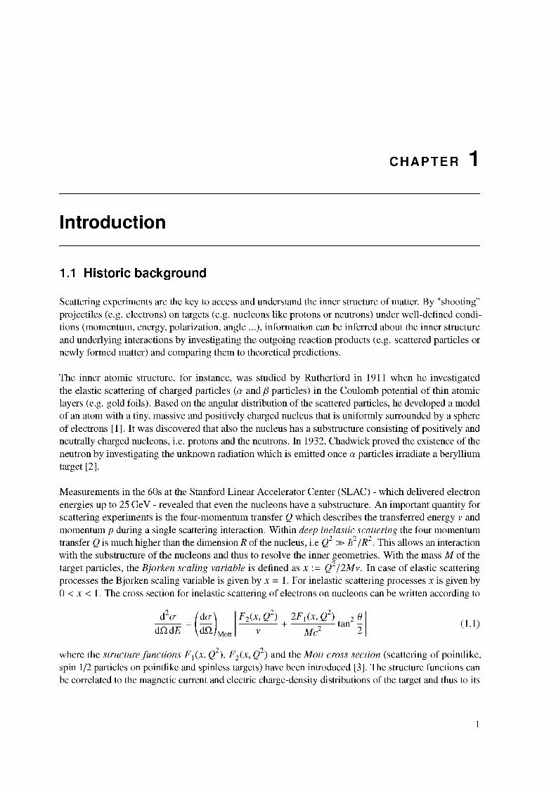
(a) Structure function F2 for the proton as a function of x and different values for Q2 [3].
Figure 1.1: Measurements of the structure function F2 for the proton and the ratio of the structure functions F1 and F2 (crosscheck of the Callan-Gross relation).
(b) Ratio of the structure functions F1 and F2 fulfilling the Callan-Gross relation, i.e. ~ 1 [4].
internal structure. For pointlike charge distributions, like for electrons, the structure function F2 turns out to be independent of the momentum transfer Q2, i.e. F2(x, Q2) ! F2(x) (also called Bjorken scaling). Measurements at SLAC showed that the structure function F2 of protons is mostly unaffected by the four momentum transfer Q (cf. Fig. 1.1(a)) which leads to the conclusion that protons and neutrons have a substructure consisting of pointlike particles.
For spin 1 /2 particles, a relation can be found between the structure functions which is also known as the Callan-Gross relation [5]: 2xF1(x) = F2(x). This relation has been confirmed as shown in Fig. 1.1(b): Protons and neutrons consist of pointlike particles with spin 1 /2. With the knowledge of the total spin of a nucleon it can be inferred that at least three or more constituents are needed. As the total electric charge of a nucleon is either q = 0 e (neutron) or q = 1 e (proton), fractional charges can be assumed.
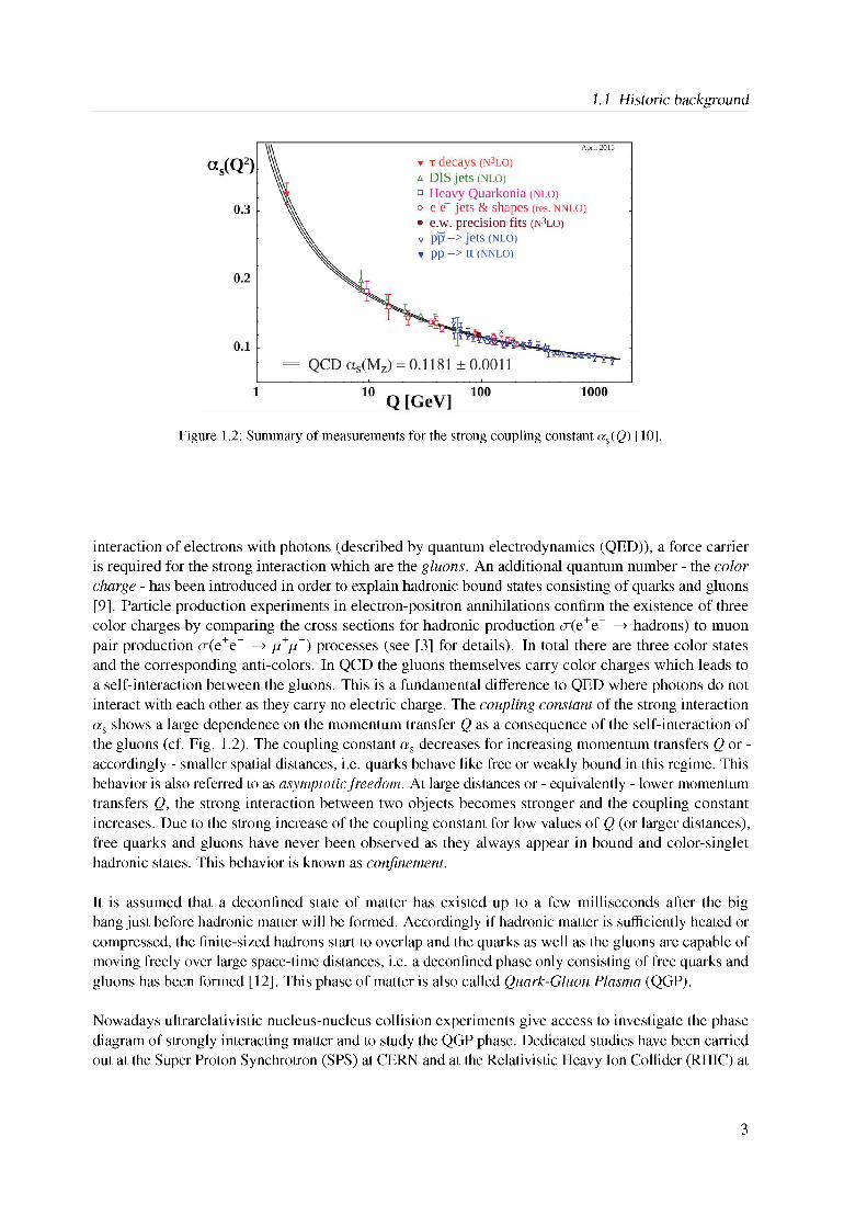
These pointlike particles are quarks. In total there are six kinds of quarks (up and down, charm and strange, top and bottom) which differ in their masses and charges. Together with the leptons (electron, muon, tau and the corresponding neutrinos) they can be arranged in three generations as shown in Fig. 1.3. Generally hadrons consisting of three quarks (i.e. qqq-states) are referred to as baryons. Quark-Antiquark states (qq) are known as mesons. As example protons consist of two up and a single down quark (uud), neutrons of two down and a single up quark (udd). These quarks which determine the quantum numbers are also called valence quarks. In addition also virtual quark-antiquark pairs (sea quarks) exist which do not affect the quantum numbers as their contributions average out to zero. The remaining bosons are the intermediating exchange particles for the fundamental forces, i.e. the weak interaction (W and Z bosons), the strong interaction (gluons) and the electromagnetic interaction (photons). The latest breakthrough in the search of the Higgs boson at CERN was rewarded with the nobel prize in 2013 for Higgs [6] and Englert [7].
The underlying relativistic field theory of the strong interaction is referred to as quantum chromodynamics (QCD) and was first introduced in the early 1970s by Fritzsch et al. [8]. Like for the electromagnetic
2
1.1 Historic background
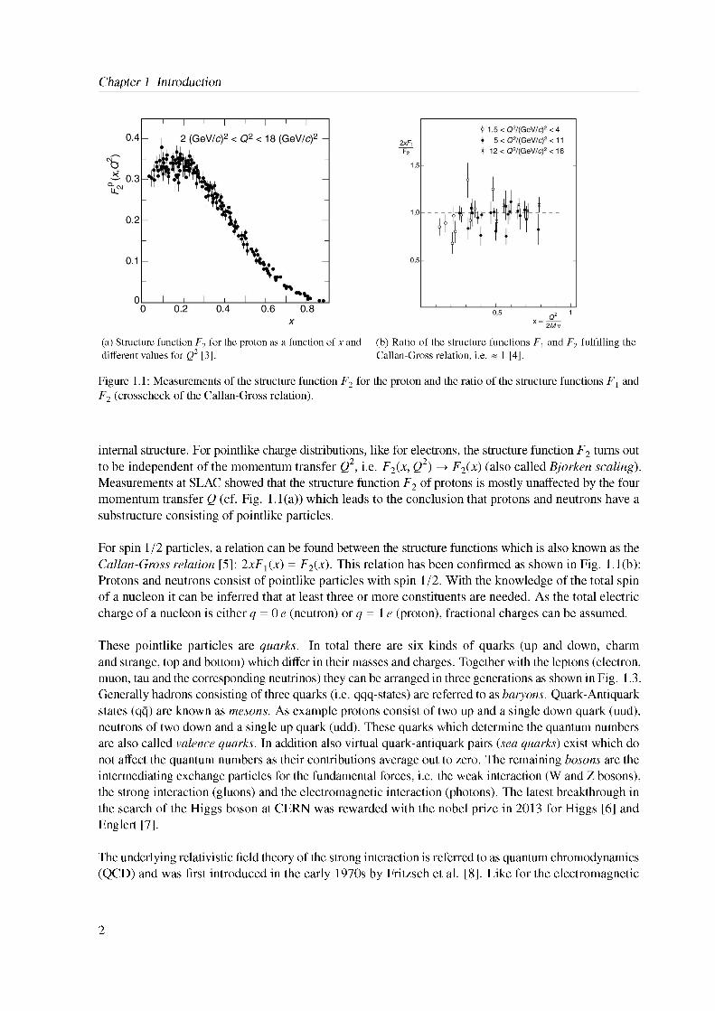
Figure 1.2: Summary of measurements for the strong coupling constant as(Q) [10].
interaction of electrons with photons (described by quantum electrodynamics (QED)), a force carrier is required for the strong interaction which are the gluons. An additional quantum number - the color charge - has been introduced in order to explain hadronic bound states consisting of quarks and gluons [9]. Particle production experiments in electron-positron annihilations confirm the existence of three color charges by comparing the cross sections for hadronic production <r(e+e~ ! hadrons) to muon pair production <r(e+e~ ! p+p”) processes (see [3] for details). In total there are three color states and the corresponding anti-colors. In QCD the gluons themselves carry color charges which leads to a self-interaction between the gluons. This is a fundamental difference to QED where photons do not interact with each other as they carry no electric charge. The coupling constant of the strong interaction as shows a large dependence on the momentum transfer Q as a consequence of the self-interaction of the gluons (cf. Fig. 1.2). The coupling constant as decreases for increasing momentum transfers Q or - accordingly - smaller spatial distances, i.e. quarks behave like free or weakly bound in this regime. This behavior is also referred to as asymptotic freedom. At large distances or - equivalently - lower momentum transfers Q, the strong interaction between two objects becomes stronger and the coupling constant increases. Due to the strong increase of the coupling constant for low values of Q (or larger distances), free quarks and gluons have never been observed as they always appear in bound and color-singlet hadronic states. This behavior is known as confinement.
It is assumed that a deconfined state of matter has existed up to a few milliseconds after the big bang just before hadronic matter will be formed. Accordingly if hadronic matter is sufficiently heated or compressed, the finite-sized hadrons start to overlap and the quarks as well as the gluons are capable of moving freely over large space-time distances, i.e. a deconfined phase only consisting of free quarks and gluons has been formed [12]. This phase of matter is also called Quark-Gluon Plasma (QGP).
Nowadays ultrarelativistic nucleus-nucleus collision experiments give access to investigate the phase diagram of strongly interacting matter and to study the QGP phase. Dedicated studies have been carried out at the Super Proton Synchrotron (SPS) at CERN and at the Relativistic Heavy Ion Collider (RHIC) at
3
Chapter 1 Introduction
Standard Model of Elementary Particlesthree generations of matter
(fermions)interactions / force carriers
charm
photonstrange
Z boson
W bosonneutrinoelectron neutrino
Figure 1.3: The Standard Model of Elementary Particles [11].
—0.511 MeV/C1 2
1 Solenoidal Tracker at RHIC2 Pioneering High Energy Nuclear Interactions Experiment
electron
e
Brookhaven (see e.g. [13] and [14] for summarized results of the STAR1 and the PHENIX2 experiments). Understanding the QCD phase diagram and the transition from hadronic matter to the Quark-Gluon Plasma is a major exploratory focus of ALICE (A Large Ion Collider Experiment). A detailed introduction to ALICE and recent results from Run 1 and Run 2 will be presented in Sec. 3.
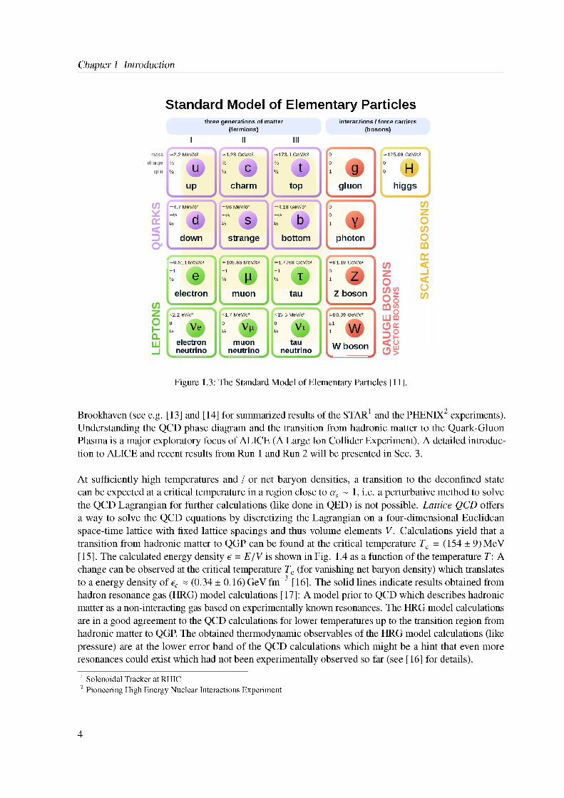
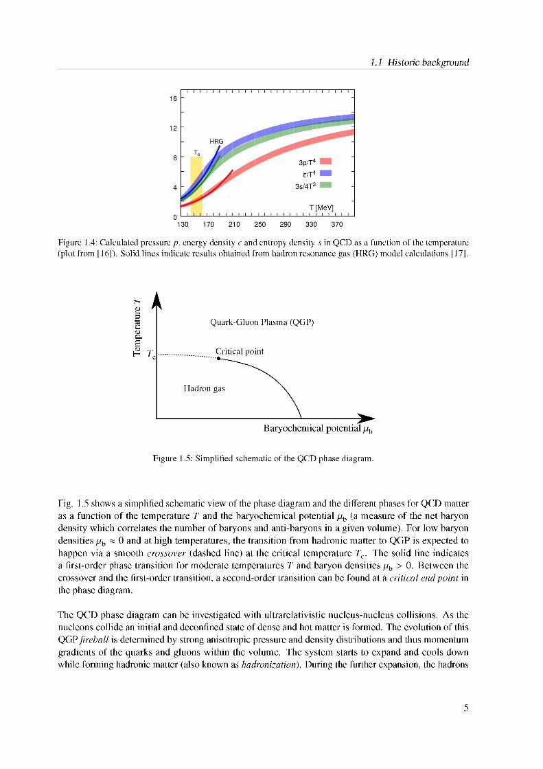
At sufficiently high temperatures and / or net baryon densities, a transition to the deconfined state can be expected at a critical temperature in a region close to as ~ 1, i.e. a perturbative method to solve the QCD Lagrangian for further calculations (like done in QED) is not possible. Lattice QCD offers a way to solve the QCD equations by discretizing the Lagrangian on a four-dimensional Euclidean space-time lattice with fixed lattice spacings and thus volume elements V. Calculations yield that a transition from hadronic matter to QGP can be found at the critical temperature Tc = (154 ± 9) MeV [15]. The calculated energy density e = E=V is shown in Fig. 1.4 as a function of the temperature T: A change can be observed at the critical temperature Tc (for vanishing net baryon density) which translates to a energy density of ec « (0.34 ± 0.16) GeV fm-3 [16]. The solid lines indicate results obtained from hadron resonance gas (HRG) model calculations [17]: A model prior to QCD which describes hadronic matter as a non-interacting gas based on experimentally known resonances. The HRG model calculations are in a good agreement to the QCD calculations for lower temperatures up to the transition region from hadronic matter to QGP. The obtained thermodynamic observables of the HRG model calculations (like pressure) are at the lower error band of the QCD calculations which might be a hint that even more resonances could exist which had not been experimentally observed so far (see [16] for details).
4
1.1 Historicbackground
Figure 1.4: Calculated pressure p, energy density e and entropy density 5 in QCD as a function of the temperature (plot from [16]). Solid lines indicate results obtained from hadron resonance gas (HRG) model calculations [17].
Figure 1.5: Simplified schematic of the QCD phase diagram.
Fig. 1.5 shows a simplified schematic view of the phase diagram and the different phases for QCD matter as a function of the temperature T and the baryochemical potential Pb (a measure of the net baryon density which correlates the number ofbaryons and anti-baryons in a given volume). For low baryon densities Pb ~ 0 and at high temperatures, the transition from hadronic matter to QGP is expected to happen via a smooth crossover (dashed line) at the critical temperature Tc. The solid line indicates a first-order phase transition for moderate temperatures T and baryon densities Pb > 0. Between the crossover and the first-order transition, a second-order transition can be found at a critical end point in the phase diagram.
The QCD phase diagram can be investigated with ultrarelativistic nucleus-nucleus collisions. As the nucleons collide an initial and deconfined state of dense and hot matter is formed. The evolution of this QGP fireball is determined by strong anisotropic pressure and density distributions and thus momentum gradients of the quarks and gluons within the volume. The system starts to expand and cools down while forming hadronic matter (also known as hadronization). During the further expansion, the hadrons
5
Chapter 1 Introduction
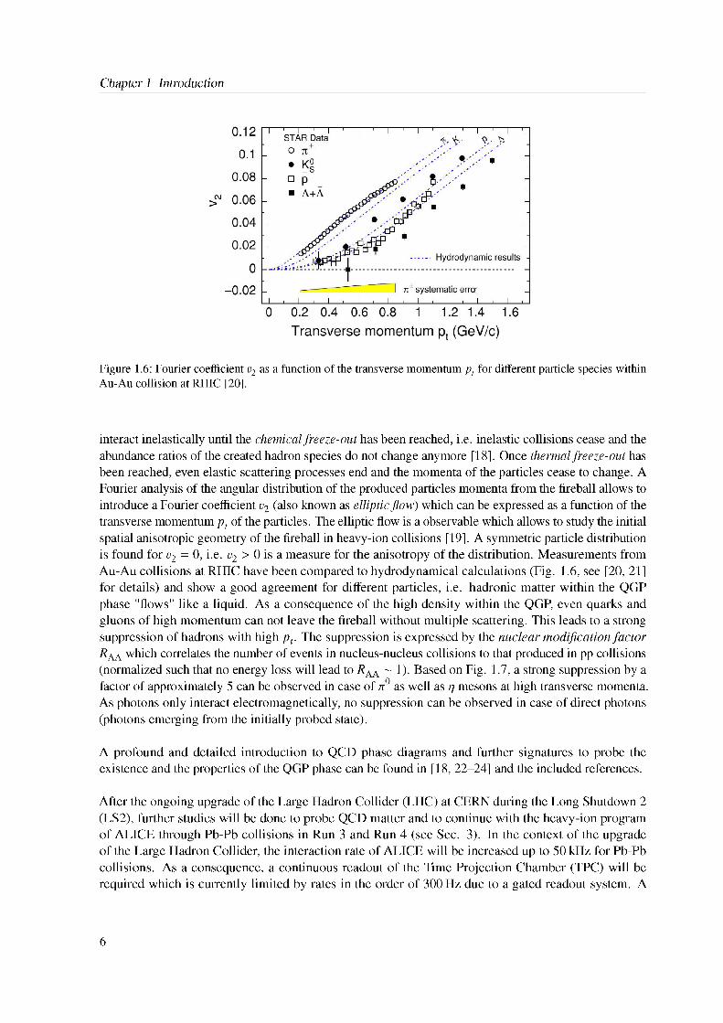
Figure 1.6: Fourier coefficient v2 as a function of the transverse momentum pt for different particle species within Au-Au collision at RHIC [20].
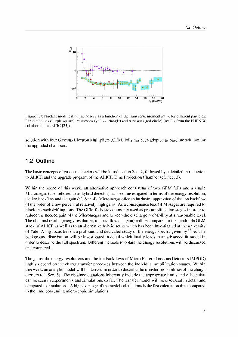
interact inelastically until the chemical freeze-out has been reached, i.e. inelastic collisions cease and the abundance ratios of the created hadron species do not change anymore [18]. Once thermal freeze-out has been reached, even elastic scattering processes end and the momenta of the particles cease to change. A Fourier analysis of the angular distribution of the produced particles momenta from the fireball allows to introduce a Fourier coefficient v2 (also known as elliptic flow) which can be expressed as a function of the transverse momentum pt of the particles. The elliptic flow is a observable which allows to study the initial spatial anisotropic geometry of the fireball in heavy-ion collisions [19]. A symmetric particle distribution is found for v2 = 0, i.e. v2 > 0 is a measure for the anisotropy of the distribution. Measurements from Au-Au collisions at RHIC have been compared to hydrodynamical calculations (Fig. 1.6, see [20, 21] for details) and show a good agreement for different particles, i.e. hadronic matter within the QGP phase "flows" like a liquid. As a consequence of the high density within the QGP, even quarks and gluons of high momentum can not leave the fireball without multiple scattering. This leads to a strong suppression of hadrons with high pt. The suppression is expressed by the nuclear modification factor Raa which correlates the number of events in nucleus-nucleus collisions to that produced in pp collisions (normalized such that no energy loss will lead to Raa ~ 1). Based on Fig. 1.7, a strong suppression by a factor of approximately 5 can be observed in case of n° as well as p mesons at high transverse momenta. As photons only interact electromagnetically, no suppression can be observed in case of direct photons (photons emerging from the initially probed state).
A profound and detailed introduction to QCD phase diagrams and further signatures to probe the existence and the properties of the QGP phase can be found in [18, 22-24] and the included references.
After the ongoing upgrade of the Large Hadron Collider (LHC) at CERN during the Long Shutdown 2 (LS2), further studies will be done to probe QCD matter and to continue with the heavy-ion program of ALICE through Pb-Pb collisions in Run 3 and Run 4 (see Sec. 3). In the context of the upgrade of the Large Hadron Collider, the interaction rate of ALICE will be increased up to 50 kHz for Pb-Pb collisions. As a consequence, a continuous readout of the Time Projection Chamber (TPC) will be required which is currently limited by rates in the order of 300 Hz due to a gated readout system. A
6
1.2 Outline
Figure 1.7: Nuclear modification factor RAA as a function of the transverse momentum pt for different particles: Direct photons (purple square), ^0 mesons (yellow triangle) and ^ mesons (red circle) (results from the PHENIX collaboration at RHIC [25]).
solution with four Gaseous Electron Multipliers (GEM) foils has been adopted as baseline solution for the upgraded chambers.
1.2 Outline
The basic concepts of gaseous detectors will be introduced in Sec. 2, followed by a detailed introduction to ALICE and the upgrade program of the ALICE Time Projection Chamber (cf. Sec. 3).
Within the scope of this work, an alternative approach consisting of two GEM foils and a single Micromegas (also referred to as hybrid detector) has been investigated in terms of the energy resolution, the ion backflow and the gain (cf. Sec. 4). Micromegas offer an intrinsic suppression of the ion backflow of the order of a few percent at relatively high gains. As a consequence less GEM stages are required to block the back drifting ions. The GEM foils are commonly used as pre-amplification stages in order to reduce the needed gain of the Micromegas and to keep the discharge probability at a reasonable level. The obtained results (energy resolution, ion backflow and gain) will be compared to the quadruple GEM stack of ALICE as well as to an alternative hybrid setup which has been investigated at the university of Yale. A big focus lies on a profound and dedicated study of the energy spectra given by 55Fe. The background distribution will be investigated in detail which finally leads to an advanced fit model in order to describe the full spectrum. Different methods to obtain the energy resolutions will be discussed and compared.
The gains, the energy resolutions and the ion backflows of Micro-Pattern Gaseous Detectors (MPGD) highly depend on the charge transfer processes between the individual amplification stages. Within this work, an analytic model will be derived in order to describe the transfer probabilities of the charge carriers (cf. Sec. 5). The obtained equations inherently include the appropriate limits and offsets that can be seen in experiments and simulations so far. The transfer model will be discussed in detail and compared to simulations. A big advantage of the model calculations is the fast calculation time compared to the time-consuming microscopic simulations.
7

Chapter 1 Introduction
The transfer probabilities give access to an in-depth study of the fundamental properties and processes within GEM stacks. Based on the transfer calculations, models will be derived in order to describe the energy resolution, the gain as well as the ion backflow for GEM stacks (cf. Sec. 6). The outcome of these calculations will be compared to measurements with the Bonn hybrid detector, the alternative hybrid setup of Yale as well as with the ALICE baseline solution based on four GEM foils.
8
CHAPTER 2
Gaseous detectors
Starting with the very first Geiger-Muller counter [26] in 1928, the invention of the Multiwire Proportional Chamber (MWPC) [27] in 1968, or the development of the Gas Electron Multiplier (GEM) [28] in 1997: Gaseous detectors have been developed and studied in numerous designs and patterns within the last decades. Nowadays they play an important role in many modern high energy physics experiments in order to identify charged particles or to reconstruct their trajectories. Though there are plenty of different designs, all gas-filled detectors are based on a common working principle: Once a charged particle traverses the active volume of the detector, different ionization processes can take place within the gas which create electron-ion pairs. The interaction of charged particles as well as of photons with matter will be discussed in Sec. 2.1 to Sec. 2.3. Commonly the created electrons are guided by electric fields to amplification stages. The movement of the charges will be part of Sec. 2.4. Usually the amount of created electrons is too small to be detected and requires an additional charge multiplication (see Sec. 2.6). The final charges are thereupon read out and allow to extract spatial information about the incident particles (cf. Sec. 2.7). The physics of these processes will be introduced and discussed in the following sections.
2.1 Interaction of charged particles with matter
Heavy charged particles interact electromagnetically with matter in multiple inelastic collision processes1. Within each individual collision a certain amount of energy is lost through atomic ionization or excitation. Within primary ionization processes of charged particles (p) with matter, electrons (e~) are liberated from the shells of the interacting atom (X):
1 Also elastic processes are possible but neglected as this does not cause noticeable energy losses.
p + X —— p + X + e . (2.1)
Some of the primary electrons are able to ionize further atoms as the remaining energy is still sufficient for additional secondary ionization processes. The kinetic energy distribution of the primary ionization electrons shows a less probable but long tail for higher energies. Electrons with very high energies from head-on collisions are emitted in forward direction. However most of the higher energetic electrons (energies of a few keV) are emitted perpendicularly to the direction of the incident particle and cause ionizations far from the track. These electrons are also referred to as delta electrons. As a consequence the resolution of gaseous detectors is limited by delta electrons. A further ionization process is the Penning effect. Once excited, some atoms are able to remain in a metastable state (X*). Through collisions with
9
Chapter 2 Gaseous detectors
Table 2.1: Average energy per produced electron-ion pair W for different gases and mixtures [30, 32].
Gas W / eV Gas mixture W / eVNe 37 Ne-CO2 (90-10) 38.1Ar 26 Ne-CO2-N2 (90-10-5) 37.3
Ar-CO2 (90-10) 28.8
atoms (Y) of a different type, a de-excitation can occur which leads to an ionization:
X* + Y ! X + Y+ + e" . (2.2)
The quantity which describes the collision probability between two successive collisions for an incoming particle is the mean free path 2. The mean free path can be correlated to the density of the electrons ne
and the collision cross section a according to 2 = 1 / (ne • a). The average amount of primary collisions within a length L is given by p = L/2 and is described by a Poisson distribution [29]. Indeed most of the electrons emerge from secondary ionization processes: For Argon and at normal temperature (20 °C) and pressure (one atm) the total amount NT = 97 cm-1 of created electron-ion pairs per centimeter of track length is larger than the amount of primary electron-ion pairs NP = 25 cm-1 (for minimum ionizing particles, also MIPs). The same holds for Neon (NT = 40 cm-1 and NP = 13 cm-1) and Carbon dioxide (Nt = 100 cm-1 and NP = 35 cm-1) [30, 31] which will be the main gases used in the framework of this PhD thesis. Within each single collision only a certain amount of energy is lost in ionization processes. The total number of ionizations NT can be expressed by the average energy to create a free electron W and the track length L according to Eq. 2.3.
W • Nt = L • (2.3)
Some example energies W for the investigated gas mixtures are listed in Table 2.1. The stopping power (-dE/dx) has been introduced as the mean energy loss per unit path length and will be part of the following section.
2.2 Energy loss
The mean energy loss per unit path length can be described by the Bethe equation (also called Bethe- Bloch equation, cf. Eq. 2.4). The equation holds for heavy (i.e. heavier than electrons) charged particles in a kinematic range of 0.1 < py < 1 000 [30].
%} = Kz2 Z1 p dx I A p2
1, 2mec2p2y2Wmax _ p2 _ Wy)2 I2 P 2 (2.4)
The absorbing material is described by the atomic number Z and the atomic mass A. The incident particle is described by the charge number z and the velocity P = v/c. Accordingly the Lorentz factor is given by y2 = 1/(1 - P2). The maximum possible energy transfer in a single collision is denoted by Wmax and the mean excitation energy of the absorbing material by I. Furthermore, the remaining constant K = 4nNAr2mec1 = 0.307075 MeV mol-1 cm2 includes NA as Avogadro’s number, the classic electron radius re, the electron mass me and the speed of light c. The average energy loss is mostly independent
10
2.2 Energy loss
py
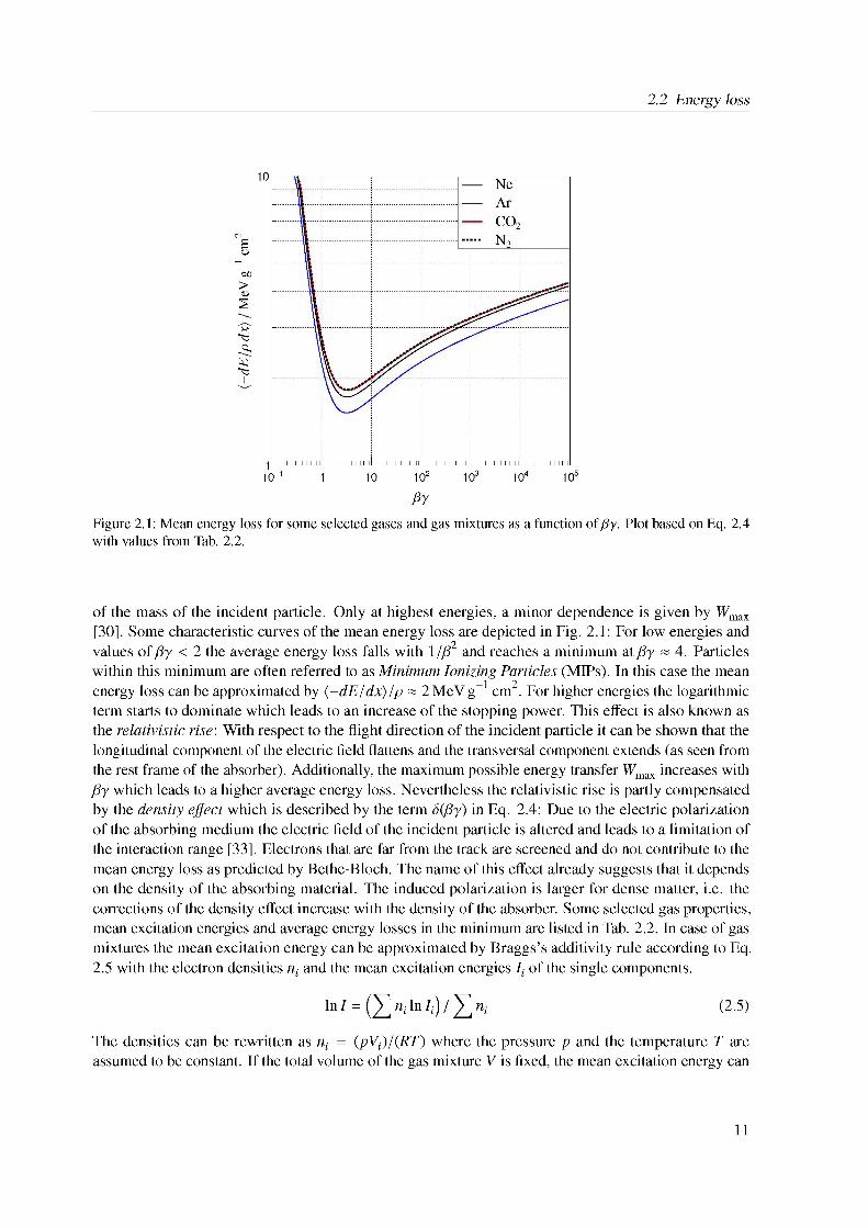
Figure 2.1: Mean energy loss for some selected gases and gas mixtures as a function of Py. Plot based on Eq. 2.4 with values from Tab. 2.2.
of the mass of the incident particle. Only at highest energies, a minor dependence is given by Wmax [30]. Some characteristic curves of the mean energy loss are depicted in Fig. 2.1: For low energies and values of Py < 2 the average energy loss falls with 1 /p2 and reaches a minimum at Py « 4. Particles within this minimum are often referred to as Minimum Ionizing Particles (MIPs). In this case the mean energy loss can be approximated by {-dE / dx) /p « 2 MeV g-1 cm2. For higher energies the logarithmic term starts to dominate which leads to an increase of the stopping power. This effect is also known as the relativistic rise: With respect to the flight direction of the incident particle it can be shown that the longitudinal component of the electric field flattens and the transversal component extends (as seen from the rest frame of the absorber). Additionally, the maximum possible energy transfer Wmax increases with Py which leads to a higher average energy loss. Nevertheless the relativistic rise is partly compensated by the density effect which is described by the term d(Py) in Eq. 2.4: Due to the electric polarization of the absorbing medium the electric field of the incident particle is altered and leads to a limitation of the interaction range [33]. Electrons that are far from the track are screened and do not contribute to the mean energy loss as predicted by Bethe-Bloch. The name of this effect already suggests that it depends on the density of the absorbing material. The induced polarization is larger for dense matter, i.e. the corrections of the density effect increase with the density of the absorber. Some selected gas properties, mean excitation energies and average energy losses in the minimum are listed in Tab. 2.2. In case of gas mixtures the mean excitation energy can be approximated by Braggs’s additivity rule according to Eq. 2.5 with the electron densities ni and the mean excitation energies Ii of the single components.
ln I = £ n, ln h) /£ „, (2.5)
The densities can be rewritten as ni = (pV,)/(RT) where the pressure p and the temperature T are assumed to be constant. If the total volume of the gas mixture V is fixed, the mean excitation energy can
11
Chapter 2 Gaseous detectors
Table 2.2: Selected atomic properties, mean excitation energies and specific ionization in the minimum [34].
Gas Z A / g mol 1 Density p / g l 1 Mean excitation energy I / eV {-dE/dx}/p / MeVg 1 cm2
Ne 10 20.18 0.90 137 1.73Ar 18 39.95 1.78 188 1.52CO2 22 44.00 1.98 85 1.83N2 14 28.01 1.25 82 1.83
be written as
ln I = fi ln Ii (2.6)
where the volume fraction is defined as f = Vi/V. The mean excitation energy of Ne-CO2 (90-10) is given by 130.6 eV. By adding Nitrogen the mean excitation energy is lowered to 127.8 eV for Ne-CO2-N2 (90-10-5). In case of Ar-CO2 (90-10) it is given by 173.7 eV.
2.3 Interaction of photons with matter
Since photons carry no electric charge they follow different interaction mechanisms with matter compared to heavy and charged particles. Generally photons are more capable of penetrating through matter due to smaller cross sections. They interact either by absorption or by scattering processes which change the intensity but not the energy of the incident beam. The intensity of the beam falls exponentially with the thickness x of the absorber according to
I (x) = I0 exp (-px) (2.7)
where I0 corresponds to the primary beam intensity. The mass absorption coefficient p can be expressed by the total cross section a and the atom density N (cf. Eq. 2.8). Like for heavy and charged particles a mean free path A can be found for the interaction of photons with matter.
p = Na = 1 (2.8)A
The main interaction mechanisms of photons in matter are the photoelectric effect, Compton scattering and pair production. The physics of the mentioned processes will be briefly summarized. A more detailed introduction can be found in [35] or [36].
2.3.1 Photoelectric effect
The photoelectric effect describes the absorption of a photon by an atomic bound electron. The electron is thereupon kicked out of the atom. Due to energy and momentum conservation, this effect can not occur for free electrons: The recoil momentum is transferred to the nucleus and the energy to the electron. The bound electron is capable of escaping from the atom if the energy of the incoming photon Ey = hv exceeds its binding energy EB. The kinetic energy E^ of the outgoing electron is given by Eq. 2.9 [37].
Ekin = Ey - Eb (2.9)
12
2.3 Interaction of photons with matter
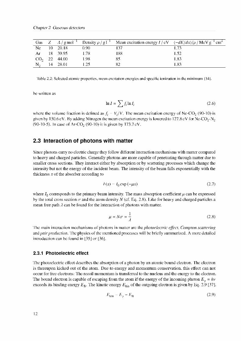
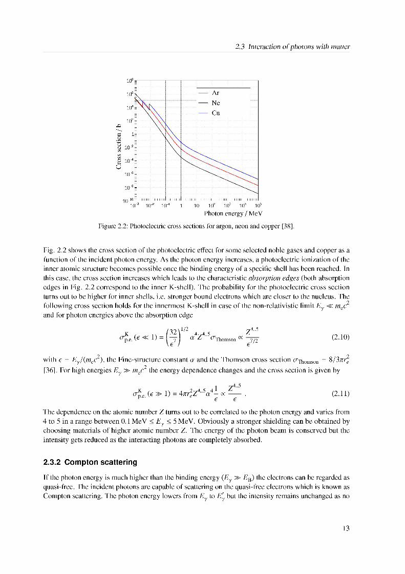
Figure 2.2: Photoelectric cross sections for argon, neon and copper [38].
Fig. 2.2 shows the cross section of the photoelectric effect for some selected noble gases and copper as a function of the incident photon energy. As the photon energy increases, a photoelectric ionization of the inner atomic structure becomes possible once the binding energy of a specific shell has been reached. In this case, the cross section increases which leads to the characteristic absorption edges (both absorption edges in Fig. 2.2 correspond to the inner K-shell). The probability for the photoelectric cross section turns out to be higher for inner shells, i.e. stronger bound electrons which are closer to the nucleus. The
2 following cross section holds for the innermost K-shell in case of the non-relativistic limit Ey ^ mec and for photon energies above the absorption edge
K ( ^u = /32 !1/2 474..5 Z 4-5p.e. (e ^ 1) 7 a Z ^Thomson / 7/2 (2.10)
with - = Ey/(mec2), the Fine-structure constant a and the Thomson cross section ^Thomson = 8/3^r2
[36]. For high energies Ey » mec2 the energy dependence changes and the cross section is given by
^Ke. (- ^ 1) = 4^r2Z4..5a4- /------ . (2.11)
The dependence on the atomic number Z turns out to be correlated to the photon energy and varies from 4 to 5 in a range between 0.1 MeV < Ey < 5 MeV. Obviously a stronger shielding can be obtained by choosing materials of higher atomic number Z. The energy of the photon beam is conserved but the intensity gets reduced as the interacting photons are completely absorbed.
2.3.2 Compton scattering
If the photon energy is much higher than the binding energy (Ey » EB) the electrons can be regarded as quasi-free. The incident photons are capable of scattering on the quasi-free electrons which is known as Compton scattering. The photon energy lowers from Ey to E'y but the intensity remains unchanged as no
13
Chapter 2 Gaseous detectors
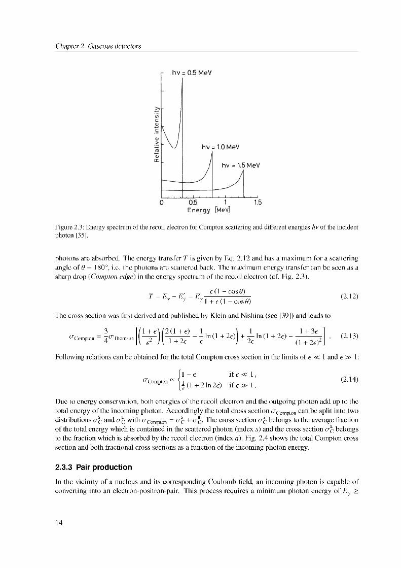
Figure 2.3: Energy spectrum of the recoil electron for Compton scattering and different energies hv of the incident photon [35].
photons are absorbed. The energy transfer T is given by Eq. 2.12 and has a maximum for a scattering angle of 6 = 180°, i.e. the photons are scattered back. The maximum energy transfer can be seen as a sharp drop (Compton edge) in the energy spectrum of the recoil electron (cf. Fig. 2.3).
, e (1 - cos 6)T = E7 - E' = E7 --------
’ ’ ’ 1 + e (1 - cos 6)
The cross section was first derived and published by Klein and Nishina (see [39]) and leads to
3cCompton 4 cThomson
2(1 + e)1 + 2e
- - ln (1 + 2e) | + ln (1 + 2e)----- + ee / 2e (1 + 2e)2J
(2.12)
(2.13)
Following relations can be obtained for the total Compton cross section in the limits of e ^ 1 and e » 1:
1 - e cCompton /j 1 (1 + 2ln2e)
if e « 1,
if e » 1.(2.14)
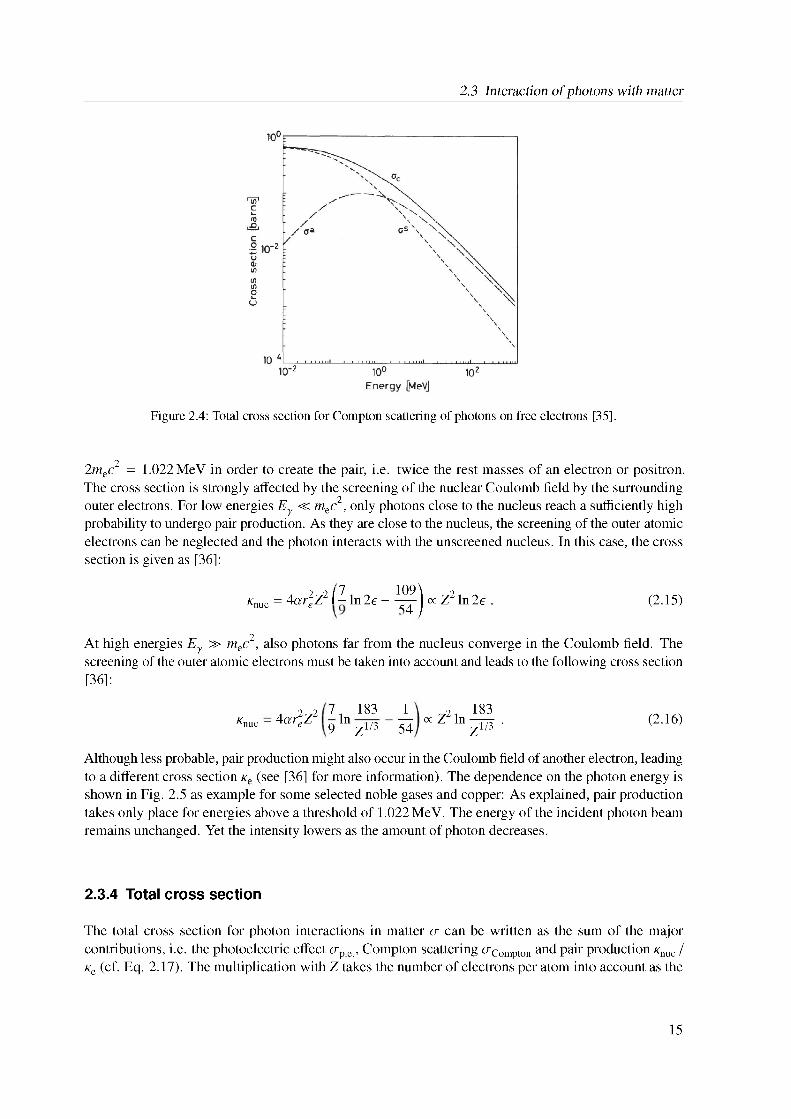
Due to energy conservation, both energies of the recoil electron and the outgoing photon add up to the total energy of the incoming photon. Accordingly the total cross section cCompton can be split into two distributions cC and cC with cCompton = cC + cjC. The cross section cC belongs to the average fraction of the total energy which is contained in the scattered photon (index 5) and the cross section cC belongs to the fraction which is absorbed by the recoil electron (index a). Fig. 2.4 shows the total Compton cross section and both fractional cross sections as a function of the incoming photon energy.
2.3.3 Pair production
In the vicinity of a nucleus and its corresponding Coulomb field, an incoming photon is capable of converting into an electron-positron-pair. This process requires a minimum photon energy of Ey >
14
2.3 Interaction of photons with matter
Figure 2.4: Total cross section for Compton scattering of photons on free electrons [35].
2mec2 = 1.022 MeV in order to create the pair, i.e. twice the rest masses of an electron or positron. The cross section is strongly affected by the screening of the nuclear Coulomb field by the surrounding outer electrons. For low energies Ey ^ mec2, only photons close to the nucleus reach a sufficiently high probability to undergo pair production. As they are close to the nucleus, the screening of the outer atomic electrons can be neglected and the photon interacts with the unscreened nucleus. In this case, the cross section is given as [36]:
*nuc = 4ar2Z2 (9 ln2e - 109 j / Z2 ffi 2e .(2.15)
At high energies Ey » meC, also photons far from the nucleus converge in the Coulomb field. The screening of the outer atomic electrons must be taken into account and leads to the following cross section [36]:
„ 2^2 A 183^nuc = 4®reZ 9 ln z1=3 ± / z^A3.
54 z1/3 (2.16)
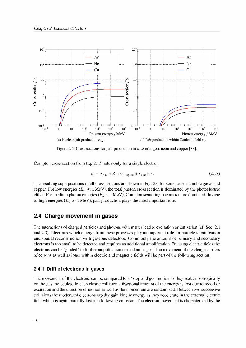
Although less probable, pair production might also occur in the Coulomb field of another electron, leading to a different cross section Ke (see [36] for more information). The dependence on the photon energy is shown in Fig. 2.5 as example for some selected noble gases and copper: As explained, pair production takes only place for energies above a threshold of 1.022 MeV. The energy of the incident photon beam remains unchanged. Yet the intensity lowers as the amount of photon decreases.
2.3.4 Total cross section
The total cross section for photon interactions in matter a can be written as the sum of the major contributions, i.e. the photoelectric effect ap.e., Compton scattering aCompton and pair production Knuc / Ke (cf. Eq. 2.17). The multiplication with Z takes the number of electrons per atom into account as the
15
Chapter 2 Gaseous detectors
Figure 2.5: Cross sections for pair production in case of argon, neon and copper [38].
Compton cross section from Eq. 2.13 holds only for a single electron.
^p.e. + Z ' ^Compton + ^nuc + Ke (2.17)
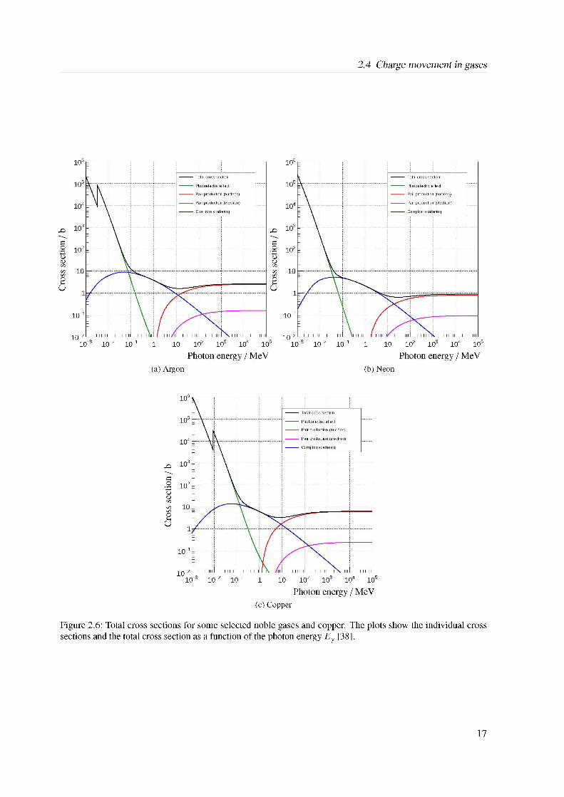
The resulting superpositions of all cross sections are shown in Fig. 2.6 for some selected noble gases and copper. For low energies (Ey ^ 1 MeV), the total photon cross section is dominated by the photoelectric effect. For medium photon energies (Ey « 1 MeV), Compton scattering becomes more dominant. In case of high energies (Ey » 1 MeV), pair production plays the most important role.
2.4 Charge movement in gases
The interactions of charged particles and photons with matter lead to excitation or ionization (cf. Sec. 2.1 and 2.3). Electrons which emerge from these processes play an important role for particle identification and spatial reconstruction with gaseous detectors. Commonly the amount of primary and secondary electrons is too small to be detected and requires an additional amplification. By using electric fields the electrons can be "guided" to further amplification or readout stages. The movement of the charge carriers (electrons as well as ions) within electric and magnetic fields will be part of the following section.
2.4.1 Drift of electrons in gases
The movement of the electrons can be compared to a "stop and go" motion as they scatter isotropically on the gas molecules. In each elastic collision a fractional amount of the energy is lost due to recoil or excitation and the direction of motion as well as the momentum are randomized. Between two successive collisions the moderated electrons rapidly gain kinetic energy as they accelerate in the external electric field which is again partially lost in a following collision. The electron movement is characterized by the
16
2.4 Charge movement in gases
Figure 2.6: Total cross sections for some selected noble gases and copper. The plots show the individual cross sections and the total cross section as a function of the photon energy E? [38].
17
Chapter 2 Gaseous detectors
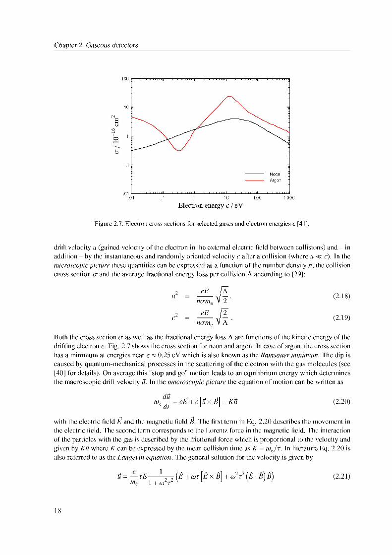
Figure 2.7: Electron cross sections for selected gases and electron energies e [41].
drift velocity u (gained velocity of the electron in the external electric field between collisions) and - in addition - by the instantaneous and randomly oriented velocity c after a collision (where u ^ c). In the microscopic picture these quantities can be expressed as a function of the number density n, the collision cross section a and the average fractional energy loss per collision A according to [29]:
eE name
eE name
u
c
(2.18)
(2.19)
Both the cross section a as well as the fractional energy loss A are functions of the kinetic energy of the drifting electron e. Fig. 2.7 shows the cross section for neon and argon. In case of argon, the cross section has a minimum at energies near e « 0.25 eV which is also known as the Ramsauer minimum. The dip is caused by quantum-mechanical processes in the scattering of the electron with the gas molecules (see [40] for details). On average this "stop and go" motion leads to an equilibrium energy which determines the macroscopic drift velocity i. In the macroscopic picture the equation of motion can be written as
me d = eE + e [^ x B] _ Kiu (2.20)
with the electric field E and the magnetic field B. The first term in Eq. 2.20 describes the movement in the electric field. The second term corresponds to the Lorentz force in the magnetic field. The interaction of the particles with the gas is described by the frictional force which is proportional to the velocity and given by Ki! where K can be expressed by the mean collision time as K = me/r. In literature Eq. 2.20 is also referred to as the Langevin equation. The general solution for the velocity is given by
(2.21)
18
i = — tE---- 1—— (E + !T [E X B] + !2t2 (E • B) B)me 1 + !2T2
2.4 Charge movement in gases
(a) Ne-CO2 (90-10) (b) Ne-CO2-N2 (90-10-5)
E / V/cm
(c) Ar-CO2 (90-10)
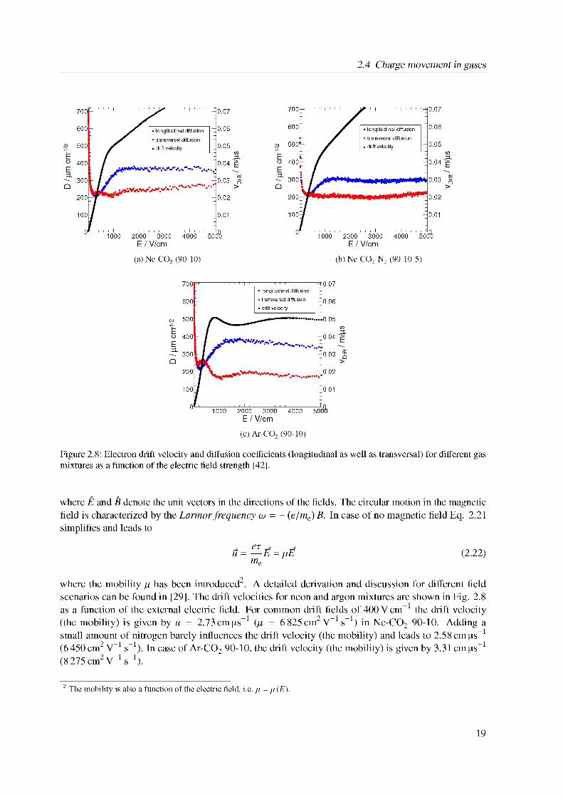
Figure 2.8: Electron drift velocity and diffusion coefficients (longitudinal as well as transversal) for different gas mixtures as a function of the electric field strength [42].
where E and B denote the unit vectors in the directions of the fields. The circular motion in the magnetic field is characterized by the Larmor frequency ! = - (e/me) B. In case of no magnetic field Eq. 2.21 simplifies and leads to
~ = EL E = gE me
(2.22)
where the mobility g has been introduced2. A detailed derivation and discussion for different field scenarios can be found in [29]. The drift velocities for neon and argon mixtures are shown in Fig. 2.8 as a function of the external electric field. For common drift fields of 400 V cm-1 the drift velocity (the mobility) is given by u = 2.73 cm ^s’1 (g = 6 825 cm2 V-1 s’1) in Ne-CO2 90-10. Adding a small amount of nitrogen barely influences the drift velocity (the mobility) and leads to 2.58 cm ^s’1
s’1). In case of Ar-CO2 90-10, the drift velocity (the mobility) is given by 3.31 cm ^s’1
s’1).
2 The mobility is also a function of the electric field, i.e. g = g (E).
(6450 cm2 V1
(8 275 cm2V-1
19
Chapter 2 Gaseous detectors
2.4.2 Drift of ions in gases
The drift motion of ions differs from electrons as they have a much higher mass. Though their energy gain in external electric fields is similar to that of electrons, they lose a larger fractional amount of energy in collisions. The ion momentum is not randomized as for electrons and ions are capable of "memorizing" their former momentum and direction. Due to this the diffusion of ions is much smaller than the diffusion of electrons as it will be discussed in Sec. 5.4.1. The mobility of ions does not vary as much as for electrons. For small electric fields (where the thermal motion can not be neglected) the drift velocity is given by [29]
u<B 1 1 H 1 !1/2 eE____ , ____ H ____ H ___I III n 7 I _\mion mgas ) \jkTf ll(T
(2.23)
and the mobility turns out to be independent of the electric field (cf. Eq. 2.22, k Boltzmann’s constant, T gas temperature, mion mass of scattering ion and mgas mass of gas molecules). For large electric fields it can be shown that [29]
u>mionm '"gas k
131/2 mion +---------m gas
/ E1/2 (2.24)0
1
Accordingly the mobility decreases as 1 / VE. The ion mobility has been measured for gas mixtures like Ar-CO2 or Ne-CO2 for different water contents and admixtures of N2. A detailed study can be found in[43] where the reduced mobility K0 (at normal temperature and pressure) and the mobility K (at given temperature TMeas and atmospheric pressure pMeas) are correlated by:
„ „ 237.15K pMeasK0 = K x--------------------x —^-Mas—
0 Tm^ 1013mbar(2.25)
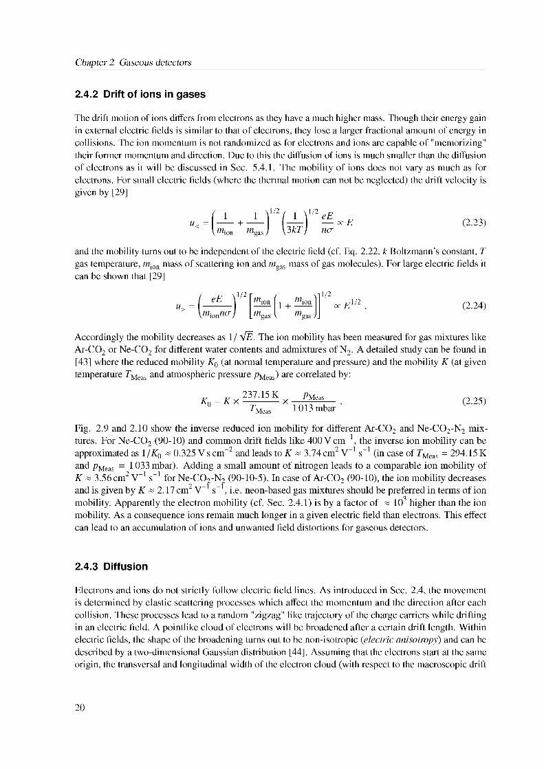
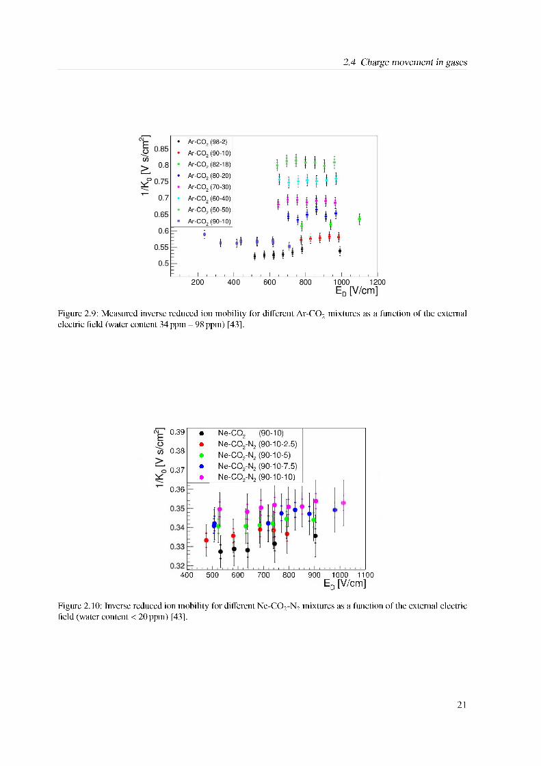
Fig. 2.9 and 2.10 show the inverse reduced ion mobility for different Ar-CO2 and Ne-CO2-N2 mixtures. For Ne-CO2 (90-10) and common drift fields like 400 V cm-1, the inverse ion mobility can be approximated as 1 /K0 ~ 0.325 V s cm-2 and leads to K ~ 3.74 cm2 V-1 s-1 (in case of TMeas = 294.15 K and pMeas = 1033 mbar). Adding a small amount of nitrogen leads to a comparable ion mobility of K ~ 3.56 cm2 V-1 s-1 for Ne-CO2-N2 (90-10-5). In case of Ar-CO2 (90-10), the ion mobility decreases and is given by K ~ 2.17 cm2 V-1 s-1, i.e. neon-based gas mixtures should be preferred in terms of ion mobility. Apparently the electron mobility (cf. Sec. 2.4.1) is by a factor of « 103 higher than the ion mobility. As a consequence ions remain much longer in a given electric field than electrons. This effect can lead to an accumulation of ions and unwanted field distortions for gaseous detectors.
2.4.3 Diffusion
Electrons and ions do not strictly follow electric field lines. As introduced in Sec. 2.4, the movement is determined by elastic scattering processes which affect the momentum and the direction after each collision. These processes lead to a random "zigzag" like trajectory of the charge carriers while drifting in an electric field. A pointlike cloud of electrons will be broadened after a certain drift length. Within electric fields, the shape of the broadening turns out to be non-isotropic (electric anisotropy) and can be described by a two-dimensional Gaussian distribution [44]. Assuming that the electrons start at the same origin, the transversal and longitudinal width of the electron cloud (with respect to the macroscopic drift
20
2.4 Charge movement in gases
Figure 2.9: Measured inverse reduced ion mobility for different Ar-CO2 mixtures as a function of the external electric field (water content 34 ppm - 98 ppm) [43].
0.39 « Ne-CO2 (90-10)• Ne-CO2-N2 (90-10-2.5)
°'38 • Ne-CO2-N2 (90-10-5)
037 • Ne-CO2-N2 (90-10-7.5)' • Ne-CO2-N2 (90-10-10)
0.36 -
400 500 600 700 800 900 1000 1100Ed [V/cm]
Figure 2.10: Inverse reduced ion mobility for different Ne-CO2-N2 mixtures as a function of the external electric field (water content < 20 ppm) [43].
21
Chapter 2 Gaseous detectors
direction) after the time t is given by
^T/L = ^ 2DT/Lt (2.26)
where the transversal DT and the longitudinal DL diffusion coefficients have been introduced. The geometric expansion of the charge cloud can be expressed as a function of the drift length zDrift. By introducing the diffusion constants Dconst;T=L = (2DT/L/vDrift)1/2, Eq. 2.26 turns into
aT/L = Dconst,T/L V-Drill ■ (2.27)
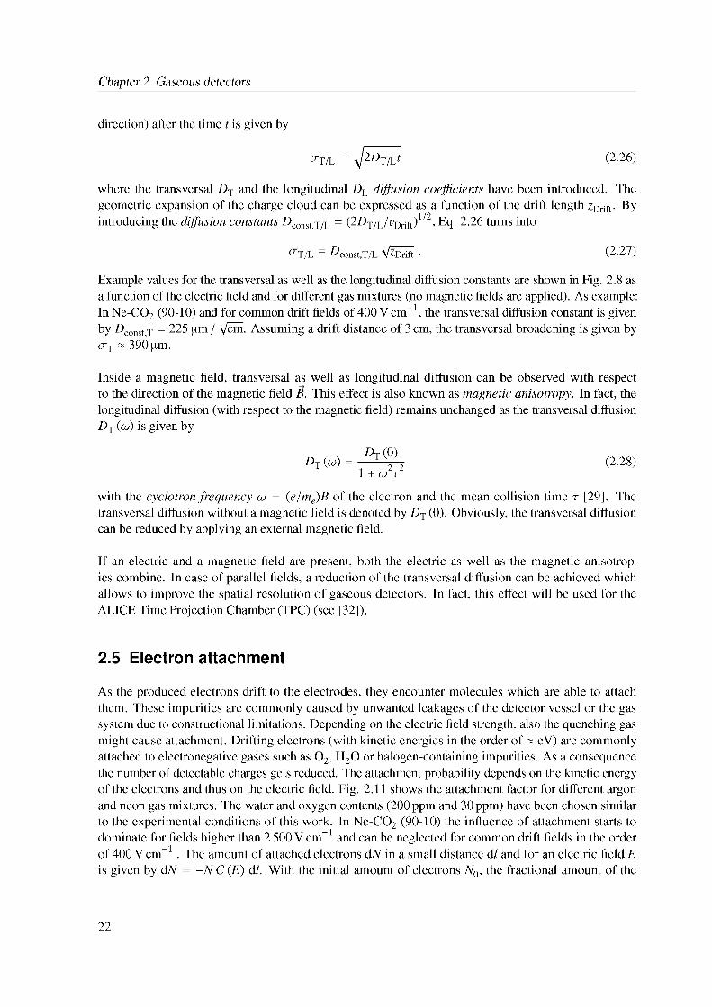
Example values for the transversal as well as the longitudinal diffusion constants are shown in Fig. 2.8 as a function of the electric field and for different gas mixtures (no magnetic fields are applied). As example: In Ne-CO2 (90-10) and for common drift fields of 400 V cm-1, the transversal diffusion constant is given by Dconst;T = 225 um / pcm. Assuming a drift distance of 3 cm, the transversal broadening is given by aT & 390 um.
Inside a magnetic field, transversal as well as longitudinal diffusion can be observed with respect to the direction of the magnetic field B. This effect is also known as magnetic anisotropy. In fact, the longitudinal diffusion (with respect to the magnetic field) remains unchanged as the transversal diffusion Dt (m) is given by
DT (0)Dt(!) = TY2 (2.28)1 + !2r2
with the cyclotron frequency m = (e/me)B of the electron and the mean collision time t [29]. The transversal diffusion without a magnetic field is denoted by DT (0). Obviously, the transversal diffusion can be reduced by applying an external magnetic field.
If an electric and a magnetic field are present, both the electric as well as the magnetic anisotropies combine. In case of parallel fields, a reduction of the transversal diffusion can be achieved which allows to improve the spatial resolution of gaseous detectors. In fact, this effect will be used for the ALICE Time Projection Chamber (TPC) (see [32]).
2.5 Electron attachment
As the produced electrons drift to the electrodes, they encounter molecules which are able to attach them. These impurities are commonly caused by unwanted leakages of the detector vessel or the gas system due to constructional limitations. Depending on the electric field strength, also the quenching gas might cause attachment. Drifting electrons (with kinetic energies in the order of ~ eV) are commonly attached to electronegative gases such as O2, H2O or halogen-containing impurities. As a consequence the number of detectable charges gets reduced. The attachment probability depends on the kinetic energy of the electrons and thus on the electric field. Fig. 2.11 shows the attachment factor for different argon and neon gas mixtures. The water and oxygen contents (200 ppm and 30 ppm) have been chosen similar to the experimental conditions of this work. In Ne-CO2 (90-10) the influence of attachment starts to dominate for fields higher than 2 500 V cm-1 and can be neglected for common drift fields in the order of 400 V cm-1 . The amount of attached electrons dN in a small distance dl and for an electric field E is given by dN = -N C (E) dl. With the initial amount of electrons N0, the fractional amount of the
22
2.6 Charge amplification and fluctuations
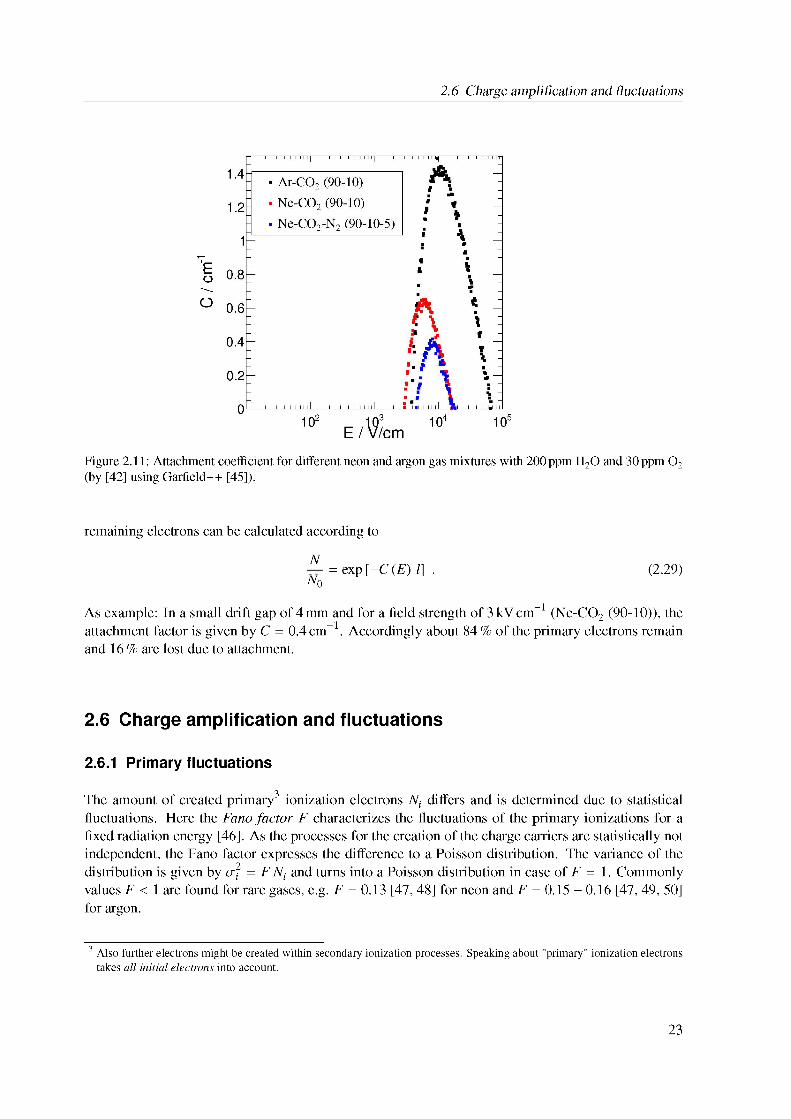
Figure 2.11: Attachment coefficient for different neon and argon gas mixtures with 200 ppm H2O and 30 ppm O2 (by [42] using Garfield++ [45]).
remaining electrons can be calculated according to
N— = exp[-C (E) l] .N0
(2.29)
As example: In a small drift gap of 4 mm and for a field strength of 3 kV cm-1 (Ne-CO2 (90-10)), the attachment factor is given by C = 0.4 cm-1. Accordingly about 84 % of the primary electrons remain and 16 % are lost due to attachment.
2.6 Charge amplification and fluctuations
2.6.1 Primary fluctuations
The amount of created primary3 ionization electrons — differs and is determined due to statistical fluctuations. Here the Fano factor F characterizes the fluctuations of the primary ionizations for a fixed radiation energy [46]. As the processes for the creation of the charge carriers are statistically not independent, the Fano factor expresses the difference to a Poisson distribution. The variance of the
2
3 Also further electrons might be created within secondary ionization processes. Speaking about "primary" ionization electrons takes all initial electrons into account.
distribution is given by at = F — and turns into a Poisson distribution in case of F = 1. Commonly values F < 1 are found for rare gases, e.g. F = 0.13 [47, 48] for neon and F = 0.15 - 0.16 [47, 49, 50] for argon.
23
Chapter 2 Gaseous detectors
2.6.2 Amplification factor I gain
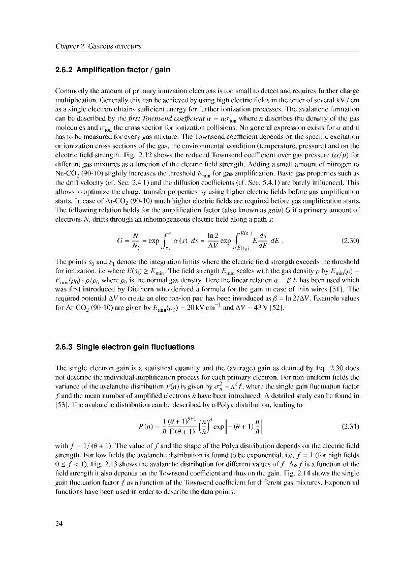
Commonly the amount of primary ionization electrons is too small to detect and requires further charge multiplication. Generally this can be achieved by using high electric fields in the order of several kV / cm as a single electron obtains sufficient energy for further ionization processes. The avalanche formation can be described by the first Townsend coefficient a = naion where n describes the density of the gas molecules and aion the cross section for ionization collisions. No general expression exists for a and it has to be measured for every gas mixture. The Townsend coefficient depends on the specific excitation or ionization cross sections of the gas, the environmental condition (temperature, pressure) and on the electric field strength. Fig. 2.12 shows the reduced Townsend coefficient over gas pressure (a/p) for different gas mixtures as a function of the electric field strength. Adding a small amount of nitrogen to Ne-CO2 (90-10) slightly increases the threshold Emin for gas amplification. Basic gas properties such as the drift velocity (cf. Sec. 2.4.1) and the diffusion coefficients (cf. Sec. 5.4.1) are barely influenced. This allows to optimize the charge transfer properties by using higher electric fields before gas amplification starts. In case of Ar-CO2 (90-10) much higher electric fields are required before gas amplification starts. The following relation holds for the amplification factor (also known as gain) G if a primary amount of electrons Ni drifts through an inhomogeneous electric field along a path s:
G = N N,
= exp f"a (s) ds = l^exp fE'S1>E^dE J-.. AV VJe(jo) dE(2.30)
The points s0 and s1 denote the integration limits where the electric field strength exceeds the threshold for ionization, i.e where E(s,) > Emin. The field strength Emin scales with the gas density p by Emin(p) = Emjn(p0)' p/p0 where p0 is the normal gas density. Here the linear relation a = fi E has been used which was first introduced by Diethorn who derived a formula for the gain in case of thin wires [51]. The required potential AV to create an electron-ion pair has been introduced as fi = ln2/AV. Example values for Ar-CO2 (90-10) are given by Emin(p0) = 20 kV cm"1 and AV = 43 V [52].
2.6.3 Single electron gain fluctuations
The single electron gain is a statistical quantity and the (average) gain as defined by Eq. 2.30 does not describe the individual amplification process for each primary electron. For non-uniform fields the variance of the avalanche distribution P(n) is given by a2 = rrf, where the single gain fluctuation factor f and the mean number of amplified electrons n have been introduced. A detailed study can be found in [53]. The avalanche distribution can be described by a Polya distribution, leading to
P (n) =1 (0 + 1)d+1 / n \d n i - Uexp - (d + 1) - n\
(2.31)
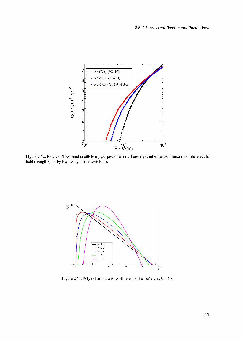
with f = 1 / (0 + 1). The value of f and the shape of the Polya distribution depends on the electric field strength. For low fields the avalanche distribution is found to be exponential, i.e. f = 1 (for high fields 0 < f < 1). Fig. 2.13 shows the avalanche distribution for different values of f. As f is a function of the field strength it also depends on the Townsend coefficient and thus on the gain. Fig. 2.14 shows the single gain fluctuation factor f as a function of the Townsend coefficient for different gas mixtures. Exponential functions have been used in order to describe the data points.
24
2.6 Charge amplification and fluctuations
Figure 2.12: Reduced Townsend coefficient / gas pressure for different gas mixtures as a function of the electric field strength (plot by [42] using Garfield++ [45]).
Figure 2.13: Polya distributions for different values of f and n = 10.
25
Chapter 2 Gaseous detectors
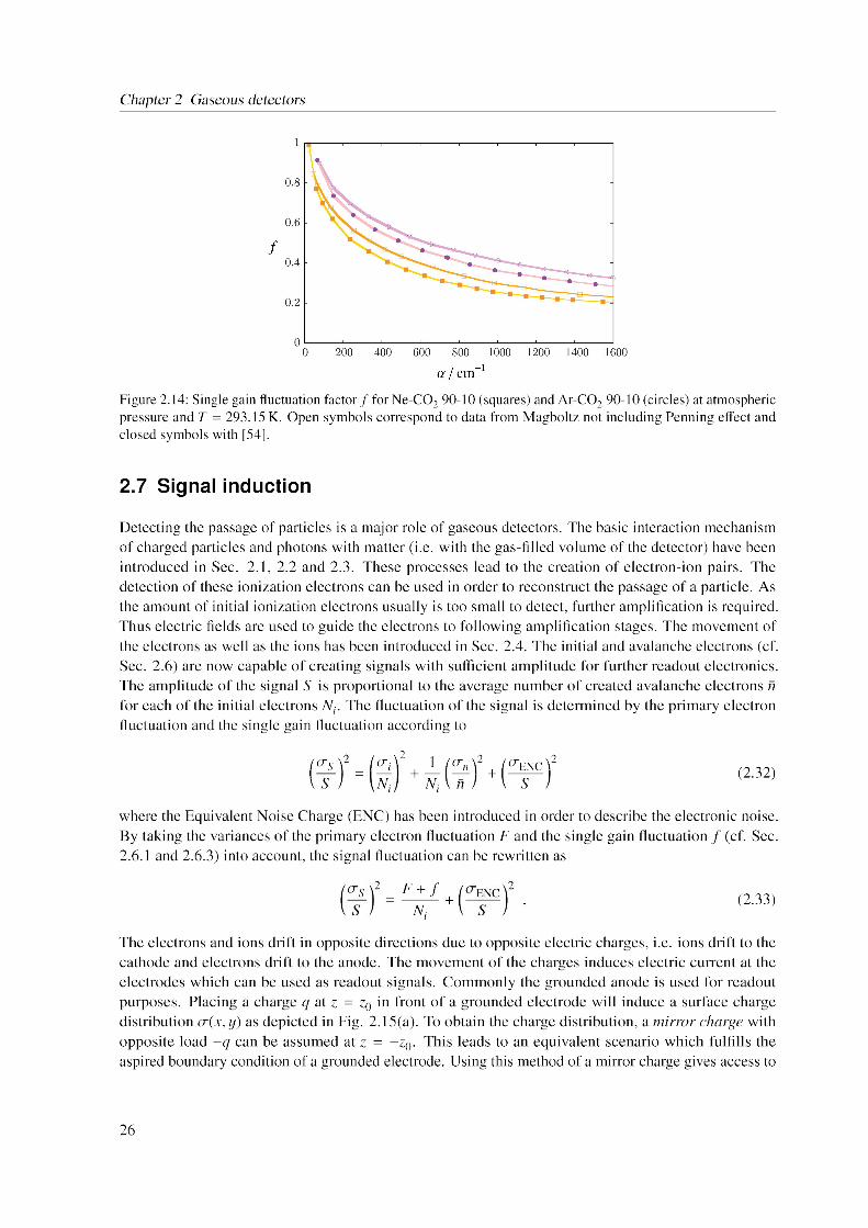
Figure 2.14: Single gain fluctuation factor f for Ne-CO2 90-10 (squares) and Ar-CO2 90-10 (circles) at atmospheric pressure and T = 293.15 K. Open symbols correspond to data from Magboltz not including Penning effect and closed symbols with [54].
2.7 Signal induction
Detecting the passage of particles is a major role of gaseous detectors. The basic interaction mechanism of charged particles and photons with matter (i.e. with the gas-filled volume of the detector) have been introduced in Sec. 2.1, 2.2 and 2.3. These processes lead to the creation of electron-ion pairs. The detection of these ionization electrons can be used in order to reconstruct the passage of a particle. As the amount of initial ionization electrons usually is too small to detect, further amplification is required. Thus electric fields are used to guide the electrons to following amplification stages. The movement of the electrons as well as the ions has been introduced in Sec. 2.4. The initial and avalanche electrons (cf. Sec. 2.6) are now capable of creating signals with sufficient amplitude for further readout electronics. The amplitude of the signal S is proportional to the average number of created avalanche electrons n for each of the initial electrons Ni. The fluctuation of the signal is determined by the primary electron fluctuation and the single gain fluctuation according to
[ts V = / Ti !2 + ± (Tn V + ( tenc \2
S N Ni n S(2.32)
where the Equivalent Noise Charge (ENC) has been introduced in order to describe the electronic noise. By taking the variances of the primary electron fluctuation F and the single gain fluctuation f (cf. Sec.2.6.1 and 2.6.3) into account, the signal fluctuation can be rewritten as
F-+f + Ni
(2.33)
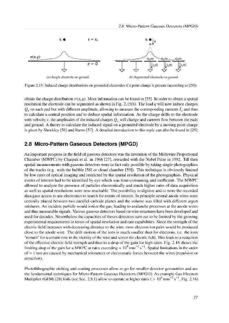
The electrons and ions drift in opposite directions due to opposite electric charges, i.e. ions drift to the cathode and electrons drift to the anode. The movement of the charges induces electric current at the electrodes which can be used as readout signals. Commonly the grounded anode is used for readout purposes. Placing a charge q at z = z0 in front of a grounded electrode will induce a surface charge distribution t(x, y) as depicted in Fig. 2.15(a). To obtain the charge distribution, a mirror charge with opposite load -q can be assumed at z = -z0. This leads to an equivalent scenario which fulfills the aspired boundary condition of a grounded electrode. Using this method of a mirror charge gives access to
26
2.8 Micro-Pattern Gaseous Detectors (MPGD)
q •
o(x,y)
z = Z0q •
Qi(t) .....Q2(t)..........Q3(t).
I3(t)
(a) Single electrode on ground. (b) Segmented electrode on ground.
z = 0
Figure 2.15: Induced charge distributions on grounded electrodes if a point charge is present (according to [29]).
obtain the charge distribution a(x, y). More information can be found in [55]. In order to obtain a spatial resolution the electrode can be segmented as shown in Fig. 2.15(b). The load q will now induce charges Qn on each pad but with different amplitude, allowing to measure the corresponding currents In and thus to calculate a central position and to deduce spatial information. As the charge drifts to the electrode with velocity v, the amplitudes of the induced charges Qn will change and currents flow between the pads and ground. A theory to calculate the induced signal on a grounded electrode by a moving point charge is given by Shockley [56] and Ramo [57]. A detailed introduction to this topic can also be found in [29].
2.8 Micro-Pattern Gaseous Detectors (MPGD)
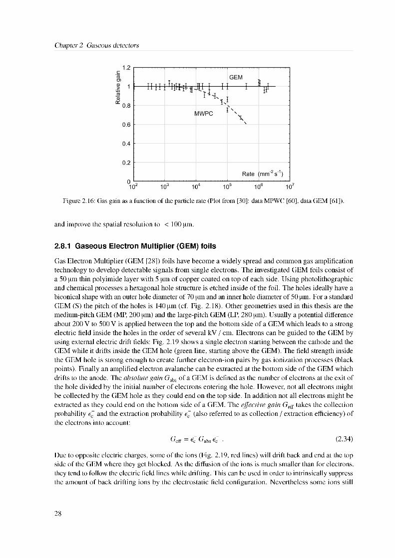
An important progress in the field of gaseous detectors was the invention of the Multiwire Proportional Chamber (MWPC) by Charpak et al. in 1968 [27], rewarded with the Nobel Prize in 1992. Till then spatial measurements with gaseous detectors were in fact only possible by taking single photographies of the tracks (e.g. with the bubble [58] or cloud chamber [59]). This technique is obviously limited by low rates of optical imaging and restricted by the spatial resolution of the photographies. Physical events of interest had to be identified by eye which was time-consuming and inefficient. The MWPC allowed to analyze the presence of particles electronically and much higher rates of data acquisition as well as spatial resolutions were now reachable. The possibility to digitize and to store the recorded data gave access to use electronics to search for events of interest. In principle several anode wires were centrally placed between two parallel cathode planes and the volume was filled with different argon mixtures. An incident particle would ionize the gas, leading to avalanche processes at the anode wires and thus measurable signals. Various gaseous detectors based on wire structures have been developed and used for decades. Nevertheless the capacities of theses detectors turn out to be limited by the growing experimental requirements in terms of spatial resolution and rate capabilities. Since the strength of the electric field increases with decreasing distance to the wire, most electron-ion pairs would be produced close to the anode wire. The drift motion of the ions is much smaller than for electrons, i.e. the ions "remain" for a certain time in the vicinity of the wire and screen the electric field. This leads to a reduction of the effective electric field strength and thus to a drop of the gain for high rates. Fig. 2.16 shows the limiting drop of the gain for a MWPC at rates exceeding ~ 104 mm-2 s-1. Spatial limitations in the order of « 1 mm are caused by mechanical tolerances or electrostatic forces between the wires (repulsion or attraction).
Photolithographic etching and coating processes allow to go for smaller detector geometries and are the fundamental techniques for Micro-Pattern Gaseous Detectors (MPGD): As example Gas Electron Multiplier (GEM) [28] foils (see Sec. 2.8.1) allow to operate at higher rates ( > 106 mm-2 s-1, Fig. 2.16)
27
Chapter 2 Gaseous detectors
Figure 2.16: Gas gain as a function of the particle rate (Plot from [30]: data MPWC [60], data GEM [61]).
and improve the spatial resolution to < 100 pm.
2.8.1 Gaseous Electron Multiplier (GEM) foils
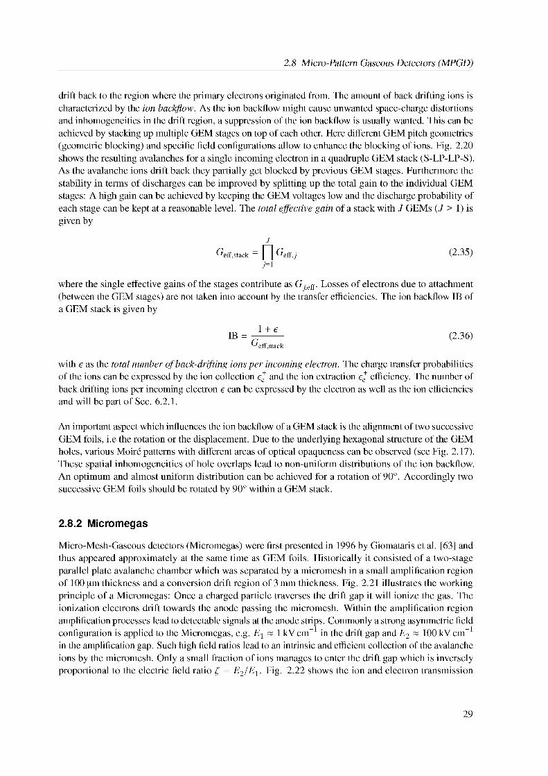
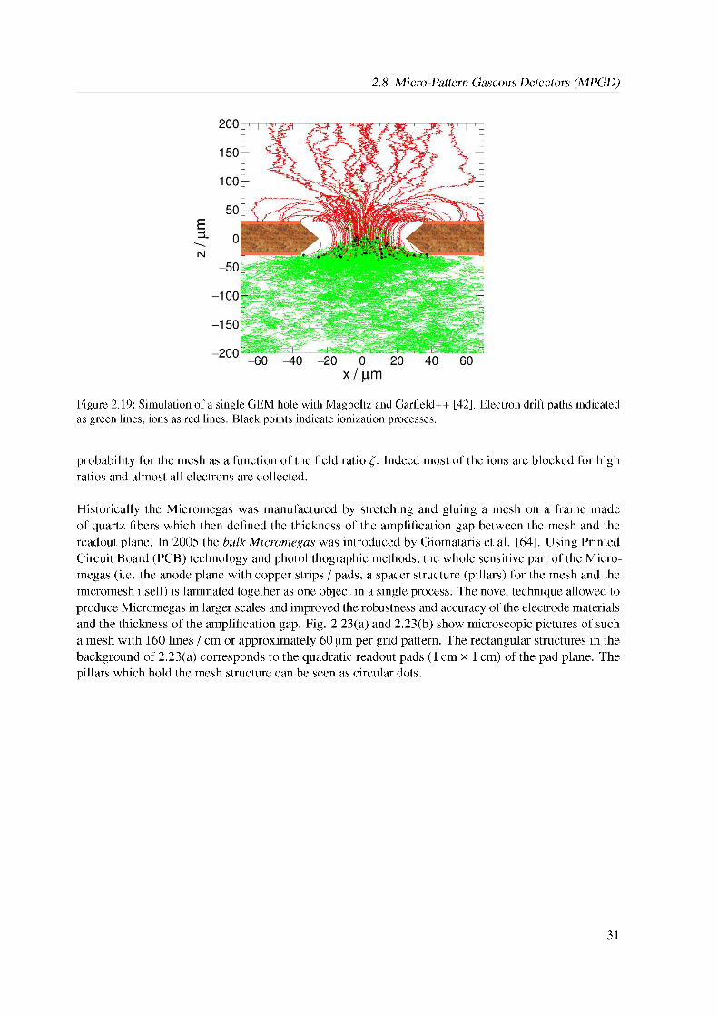
Gas Electron Multiplier (GEM [28]) foils have become a widely spread and common gas amplification technology to develop detectable signals from single electrons. The investigated GEM foils consist of a 50 pm thin polyimide layer with 5 pm of copper coated on top of each side. Using photolithographic and chemical processes a hexagonal hole structure is etched inside of the foil. The holes ideally have a biconical shape with an outer hole diameter of 70 pm and an inner hole diameter of 50 pm. For a standard GEM (S) the pitch of the holes is 140 pm (cf. Fig. 2.18). Other geometries used in this thesis are the medium-pitch GEM (MP, 200 pm) and the large-pitch GEM (LP, 280 pm). Usually a potential difference about 200 V to 500 V is applied between the top and the bottom side of a GEM which leads to a strong electric field inside the holes in the order of several kV / cm. Electrons can be guided to the GEM by using external electric drift fields: Fig. 2.19 shows a single electron starting between the cathode and the GEM while it drifts inside the GEM hole (green line, starting above the GEM). The field strength inside the GEM hole is strong enough to create further electron-ion pairs by gas ionization processes (black points). Finally an amplified electron avalanche can be extracted at the bottom side of the GEM which drifts to the anode. The absolute gain Gabs of a GEM is defined as the number of electrons at the exit of the hole divided by the initial number of electrons entering the hole. However, not all electrons might be collected by the GEM hole as they could end on the top side. In addition not all electrons might be extracted as they could end on the bottom side of a GEM. The effective gain Geff takes the collection probability e~ and the extraction probability e~ (also referred to as collection / extraction efficiency) of the electrons into account:
Geff = < Gabs < • (2.34)
Due to opposite electric charges, some of the ions (Fig. 2.19, red lines) will drift back and end at the top side of the GEM where they get blocked. As the diffusion of the ions is much smaller than for electrons, they tend to follow the electric field lines while drifting. This can be used in order to intrinsically suppress the amount of back drifting ions by the electrostatic field configuration. Nevertheless some ions still
28
2.8 Micro-Pattern Gaseous Detectors (MPGD)
drift back to the region where the primary electrons originated from. The amount of back drifting ions is characterized by the ion backflow. As the ion backflow might cause unwanted space-charge distortions and inhomogeneities in the drift region, a suppression of the ion backflow is usually wanted. This can be achieved by stacking up multiple GEM stages on top of each other. Here different GEM pitch geometries (geometric blocking) and specific field configurations allow to enhance the blocking of ions. Fig. 2.20 shows the resulting avalanches for a single incoming electron in a quadruple GEM stack (S-LP-LP-S). As the avalanche ions drift back they partially get blocked by previous GEM stages. Furthermore the stability in terms of discharges can be improved by splitting up the total gain to the individual GEM stages: A high gain can be achieved by keeping the GEM voltages low and the discharge probability of each stage can be kept at a reasonable level. The total effective gain of a stack with J GEMs (J > 1) is given by
j
Geff,stack Geff,j (2.35)
where the single effective gains of the stages contribute as Gj,eff. Losses of electrons due to attachment (between the GEM stages) are not taken into account by the transfer efficiencies. The ion backflow IB of a GEM stack is given by
IB = , 1 ' ' (2.36)Geff,stack
with e as the total number of back-drifting ions per incoming electron. The charge transfer probabilities of the ions can be expressed by the ion collection e+ and the ion extraction e+ efficiency. The number of back drifting ions per incoming electron e can be expressed by the electron as well as the ion efficiencies and will be part of Sec. 6.2.1.
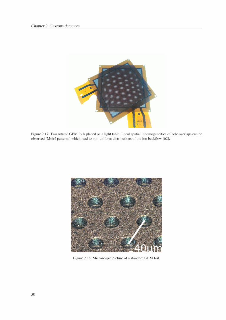
An important aspect which influences the ion backflow of a GEM stack is the alignment of two successive GEM foils, i.e the rotation or the displacement. Due to the underlying hexagonal structure of the GEM holes, various Moire patterns with different areas of optical opaqueness can be observed (see Fig. 2.17). These spatial inhomogeneities of hole overlaps lead to non-uniform distributions of the ion backflow. An optimum and almost uniform distribution can be achieved for a rotation of 90°. Accordingly two successive GEM foils should be rotated by 90° within a GEM stack.
2.8.2 Micromegas
Micro-Mesh-Gaseous detectors (Micromegas) were first presented in 1996 by Giomataris et al. [63] and thus appeared approximately at the same time as GEM foils. Historically it consisted of a two-stage parallel plate avalanche chamber which was separated by a micromesh in a small amplification region of 100 pm thickness and a conversion drift region of 3 mm thickness. Fig. 2.21 illustrates the working principle of a Micromegas: Once a charged particle traverses the drift gap it will ionize the gas. The ionization electrons drift towards the anode passing the micromesh. Within the amplification region amplification processes lead to detectable signals at the anode strips. Commonly a strong asymmetric field configuration is applied to the Micromegas, e.g. E1 ~ 1 kV cm-1 in the drift gap and E2 ~ 100 kV cm-1
in the amplification gap. Such high field ratios lead to an intrinsic and efficient collection of the avalanche ions by the micromesh. Only a small fraction of ions manages to enter the drift gap which is inversely proportional to the electric field ratio £ = E2/E1. Fig. 2.22 shows the ion and electron transmission
29
Chapter 2 Gaseous detectors
Figure 2.17: Two rotated GEM foils placed on a light table. Local spatial inhomogeneities of hole overlaps can be observed (Moire patterns) which lead to non-uniform distributions of the ion backflow [62].
Figure 2.18: Microscopic picture of a standard GEM foil.
30
2.8 Micro-Pattern Gaseous Detectors (MPGD)
Figure 2.19: Simulation of a single GEM hole with Magboltz and Garfield++ [42]. Electron drift paths indicated as green lines, ions as red lines. Black points indicate ionization processes.
probability for the mesh as a function of the field ratio £: Indeed most of the ions are blocked for high ratios and almost all electrons are collected.
Historically the Micromegas was manufactured by stretching and gluing a mesh on a frame made of quartz fibers which then defined the thickness of the amplification gap between the mesh and the readout plane. In 2005 the bulk Micromegas was introduced by Giomataris et al. [64]. Using Printed Circuit Board (PCB) technology and photolithographic methods, the whole sensitive part of the Micromegas (i.e. the anode plane with copper strips / pads, a spacer structure (pillars) for the mesh and the micromesh itself) is laminated together as one object in a single process. The novel technique allowed to produce Micromegas in larger scales and improved the robustness and accuracy of the electrode materials and the thickness of the amplification gap. Fig. 2.23(a) and 2.23(b) show microscopic pictures of such a mesh with 160 lines / cm or approximately 60 pm per grid pattern. The rectangular structures in the background of 2.23(a) corresponds to the quadratic readout pads (1cm x 1 cm) of the pad plane. The pillars which hold the mesh structure can be seen as circular dots.
31
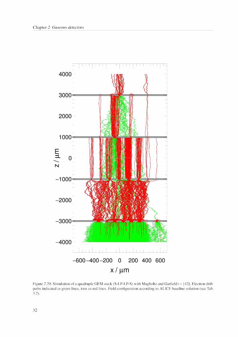
Chapter 2 Gaseous detectors
Figure 2.20: Simulation of a quadruple GEM stack (S-LP-LP-S) with Magboltz and Garfield++ [42]. Electron drift paths indicated as green lines, ions as red lines. Field configuration according to ALICE baseline solution (see Tab. 3.2).
32
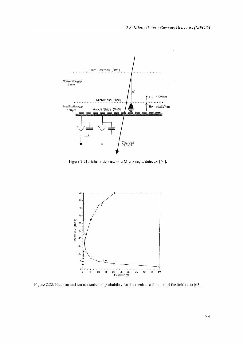
2.8 Micro-PatternGaseousDetectors(MPGD)
Figure 2.21: Schematic view of a Micromegas detector [63].
Figure 2.22: Electron and ion transmission probability for the mesh as a function of the field ratio [63].
33
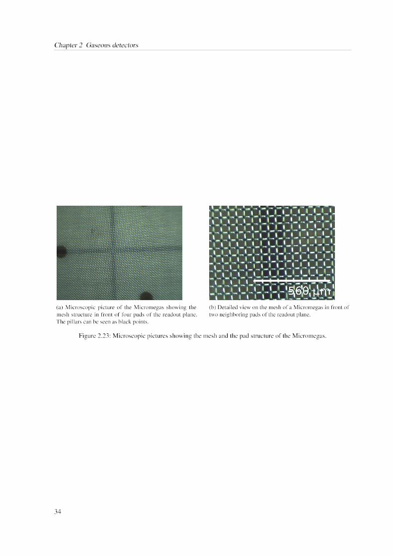
Chapter 2 Gaseous detectors
(a) Microscopic picture of the Micromegas showing the (b) Detailed view on the mesh of a Micromegas in front ofmesh structure in front of four pads of the readout plane. two neighboring pads of the readout plane.The pillars can be seen as black points.
Figure 2.23: Microscopic pictures showing the mesh and the pad structure of the Micromegas.
34
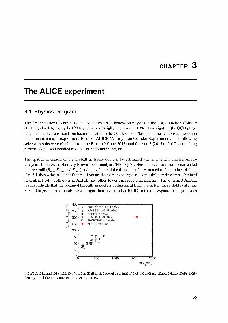
CHAPTER 3
The ALICE experiment
3.1 Physics program
The first intentions to build a detector dedicated to heavy-ion physics at the Large Hadron Collider (LHC) go back to the early 1990s and were officially approved in 1996: Investigating the QCD phase diagram and the transition from hadronic matter to the Quark-Gluon Plasma in ultra-relativistic heavy-ion collisions is a major exploratory focus of ALICE (A Large Ion Collider Experiment). The following selected results were obtained from the Run 1 (2010 to 2013) and the Run 2 (2015 to 2017) data taking periods. A full and detailed review can be found in [65, 66].
The spatial extension of the fireball at freeze-out can be estimated via an intensity interferometry analysis also know as Hanbury Brown-Twiss analysis (HBT) [67]. Here the extension can be correlated to three radii (Rout, Rlong and Rside) and the volume of the fireball can be estimated as the product of them. Fig. 3.1 shows the product of the radii versus the average charged-track multiplicity density as obtained in central Pb-Pb collisions at ALICE and other lower energetic experiments. The obtained ALICE results indicate that the obtained fireballs in nuclear collisions at LHC are hotter, more stable (lifetime t & 10fm/c, approximately 20% longer than measured at RHIC [65]) and expand to larger scales
CC
cc0C
E A350 7
300 7□
250-
200-
150 -
10OP
E895 2.7, 3.3, 3,8, 4.3 GeV NA49 8.7, 12.5,17.3 GeVCERES 17.3 GeVSTAR 62.4, 200 GeV PHOBOS 62.4, 200 GeV ALICE 2760 GeV
400
Figure 3.1: Estimated extension of the fireball at freeze-out as a function of the average charged-track multiplicity density for different center-of-mass energies [68].
35
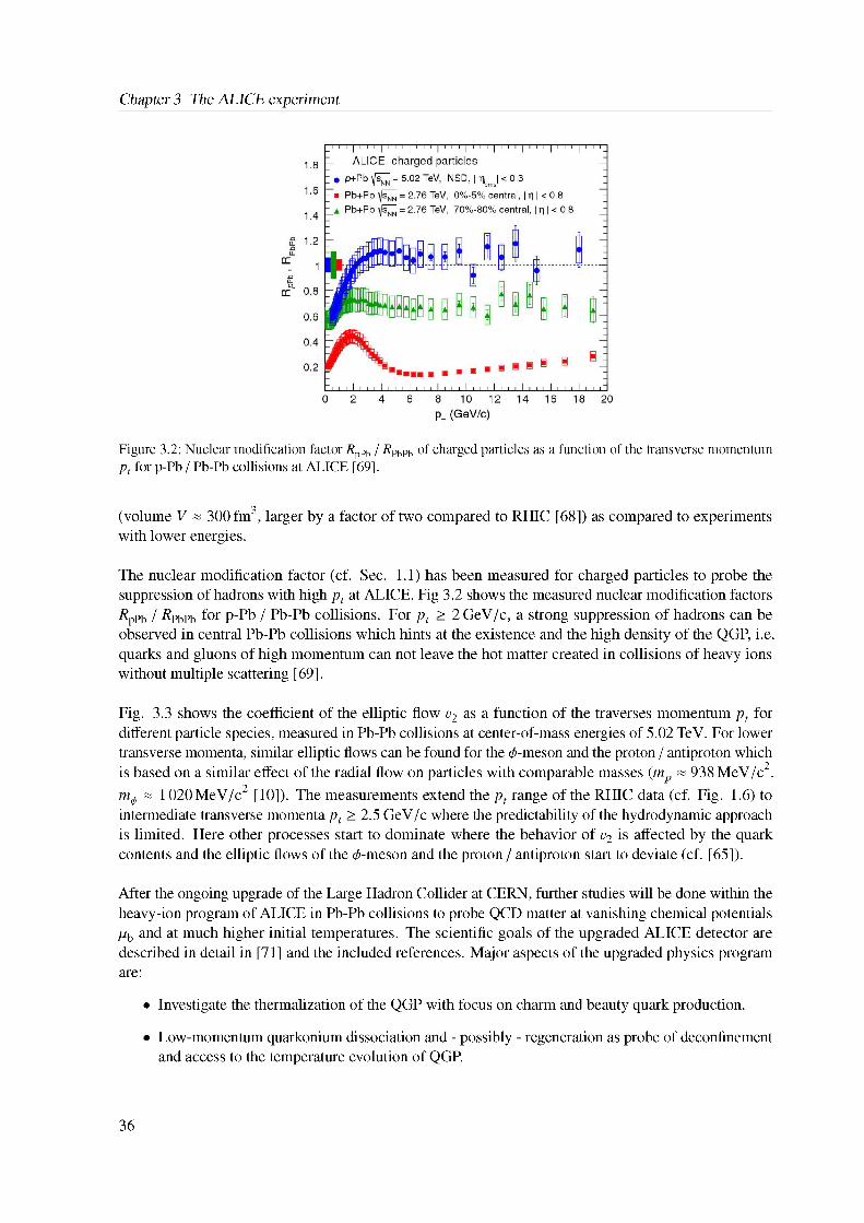
Chapter 3 The ALICE experiment
Figure 3.2: Nuclear modification factor ApPb / APbPb of charged particles as a function of the transverse momentum pt for p-Pb / Pb-Pb collisions at ALICE [69].
(volume V « 300 fm3, larger by a factor of two compared to RHIC [68]) as compared to experiments with lower energies.
The nuclear modification factor (cf. Sec. 1.1) has been measured for charged particles to probe the suppression of hadrons with high pt at ALICE. Fig 3.2 shows the measured nuclear modification factors RpPb / ^PbPb for p-Pb / Pb-Pb collisions. For pt > 2 GeV/c, a strong suppression of hadrons can be observed in central Pb-Pb collisions which hints at the existence and the high density of the QGP, i.e. quarks and gluons of high momentum can not leave the hot matter created in collisions of heavy ions without multiple scattering [69].
Fig. 3.3 shows the coefficient of the elliptic flow v2 as a function of the traverses momentum pt for different particle species, measured in Pb-Pb collisions at center-of-mass energies of 5.02 TeV. For lower transverse momenta, similar elliptic flows can be found for the 0-meson and the proton / antiproton which is based on a similar effect of the radial flow on particles with comparable masses (mp « 938 MeV/c2,
2m^ & 1020 MeV/c [10]). The measurements extend the pt range of the RHIC data (cf. Fig. 1.6) to intermediate transverse momenta pt > 2.5 GeV/c where the predictability of the hydrodynamic approach is limited. Here other processes start to dominate where the behavior of v2 is affected by the quark contents and the elliptic flows of the 0-meson and the proton / antiproton start to deviate (cf. [65]).
After the ongoing upgrade of the Large Hadron Collider at CERN, further studies will be done within the heavy-ion program of ALICE in Pb-Pb collisions to probe QCD matter at vanishing chemical potentials pb and at much higher initial temperatures. The scientific goals of the upgraded ALICE detector are described in detail in [71] and the included references. Major aspects of the upgraded physics program are:
• Investigate the thermalization of the QGP with focus on charm and beauty quark production.
• Low-momentum quarkonium dissociation and - possibly - regeneration as probe of deconfinement and access to the temperature evolution of QGP.
36
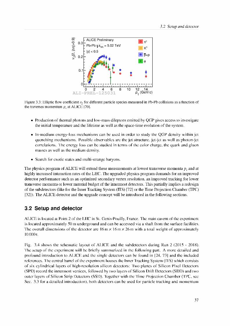
3.2 Setup and detector
Figure 3.3: Elliptic flow coefficient v2 for different particle species measured in Pb-Pb collisions as a function of the traverses momentum pt at ALICE [70].
• Production of thermal photons and low-mass dileptons emitted by QGP gives access to investigate the initial temperature and the lifetime as well as the space-time evolution of the system.
• In-medium energy-loss mechanisms can be used in order to study the QGP density within jet quenching mechanisms. Possible observables are the jet structure, jet-jet as well as photon-jet correlations. The energy loss can be studied in terms of the color charge, the quark and gluon masses as well as the medium density.
• Search for exotic states and multi-strange baryons.
The physics program of ALICE will extend these measurements at lowest transverse momenta pt and at highly increased interaction rates of the LHC. The upgraded physics program demands for an improved detector performance such as an optimized secondary vertex resolution, an improved tracking for lower transverse momenta or lower material budget of the innermost detectors. This partially implies a redesign of the subdetectors (like for the Inner Tracking System (ITS) [72] or the Time Projection Chamber (TPC) [32]). The ALICE detector and the upgrade concept will be introduced in the following sections.
3.2 Setup and detector
ALICE is located at Point 2 of the LHC in St. Genis-Pouilly, France. The main cavern of the experiment is located approximately 50 m underground and can be accessed via a shaft from the surface facilities. The overall dimensions of the detector are 16m x 16m x 26m with a total weight of approximately 10 0001.
Fig. 3.4 shows the schematic layout of ALICE and the subdetectors during Run 2 (2015 - 2018). The setup of the experiment will be briefly summarized in the following part. A more detailed and profound introduction to ALICE and the single detectors can be found in [24, 73] and the included references. The central barrel of the experiment houses the Inner Tracking System (ITS) which consists of six cylindrical layers of high-resolution silicon detectors: Two planes of Silicon Pixel Detectors (SPD) record the innermost vertices, followed by two layers of Silicon Drift Detectors (SDD) and two outer layers of Silicon Strip Detectors (SSD). Together with the Time Projection Chamber (TPC, see Sec. 3.3 for a detailed introduction), both detectors can be used for particle tracking and momentum
37
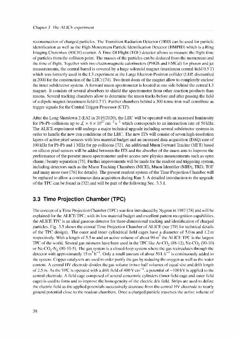
Chapter 3 The ALICE experiment
reconstruction of charged particles. The Transition Radiation Detector (TRD) can be used for particle identification as well as the High Momentum Particle Identification Detector (HMPID) which is a Ring Imaging Cherenkov (RICH) counter. A Time Of Flight (TOF) detector allows to measure the flight time of particles from the collision point. The masses of the particles can be deduced from the momentum and the time of flight. Together with two electromagnetic calorimeters (PHOS and EMCal) for photon and jet measurements, the central barrel is covered by a huge solenoid magnet (maximum central field 0.5 T) which was formerly used in the L3 experiment at the Large Electron-Positron collider (LEP, dismantled in 2000 for the construction of the LHC) [74]. Two front doors of the magnet allow to completely enclose the inner subdetector system. A forward muon spectrometer is located at one side behind the central L3 magnet. It consists of several absorbers to shield the spectrometer from other reaction products than muons. Several tracking chambers allow to determine the muon tracks before and after passing the field of a dipole magnet (maximum field 0.7 T). Further chambers behind a 300 tonne iron wall contribute as trigger signals for the Central Trigger Processor (CTP).
After the Long Shutdown 2 (LS2 in 2019/2020), the LHC will be operated with an increased luminosity for Pb-Pb collisions up to L = 6 X 1027 cm-2 s-1 which corresponds to an interaction rate of 50 kHz. The ALICE experiment will undergo a major technical upgrade including several subdetector systems in order to handle the new run conditions of the LHC. The new ITS will consist of seven high-resolution layers of active pixel sensors with less material budget and an increased data acquisition (DAQ) rate of 100 kHz for Pb-Pb and 1 MHz for pp collisions [72]. An additional Muon Forward Tracker (MFT) based on silicon pixel sensors will be added between the ITS and the absorber of the muon arm to improve the performance of the present muon spectrometer and to access new physics measurements such as open charm / beauty separation [75]. Further improvements will be made for the readout and triggering system, including detectors such as the Muon Tracking Chambers (MCH), Muon Identifier (MID), TRD, TOF and many more (see [76] for details). The present readout system of the Time Projection Chamber will be replaced to allow a continuous data acquisition during Run 3. A detailed introduction to the upgrade of the TPC can be found in [32] and will be part of the following Sec. 3.3.1.
3.3 Time Projection Chamber (TPC)
The concept of a Time Projection Chamber (TPC) was first introduced by Nygren in 1987 [78] and will be explained for the ALICE TPC; with its low material budget and excellent pattern recognition capabilities, the ALICE TPC is an ideal gaseous detector for three-dimensional tracking and identification of charged particles. Fig. 3.5 shows the central Time Projection Chamber of ALICE (see [79] for technical details of the TPC design). The outer and inner cylindrical field cages have a diameter of 5.0 m and 1.2 m respectively. With a length of 5.5 m and an active volume of about 90 m3 the ALICE TPC is the largest TPC of the world. Several gas mixtures have been used in the TPC like Ar-CO2 (88-12), Ne-CO2 (90-10) or Ne-CO2-N2 (90-10-5). The gas system is a closed-loop system where the gas recirculates through the detector with approximately 15 m3 h-1. Only a small amount of about 50 Lh-1 is continuously added to the system. Copper catalyzers are used in order purify the gas by reducing the oxygen as well as the water content. A central HV electrode divides the gas volume in two half volumes of equal size and drift length of 2.5 m. As the TPC is operated with a drift field of 400 V cm-1, a potential of -100 kV is applied to the central electrode. A field cage composed of several concentric cylinders (inner field cage and outer field cage) is used to form and to improve the homogeneity of the electric drit field. Strips are used to define the electric field as the applied potentials successively decrease from the central HV electrode to nearly ground potential close to the readout chambers. Once a charged particle traverses the active volume of
38
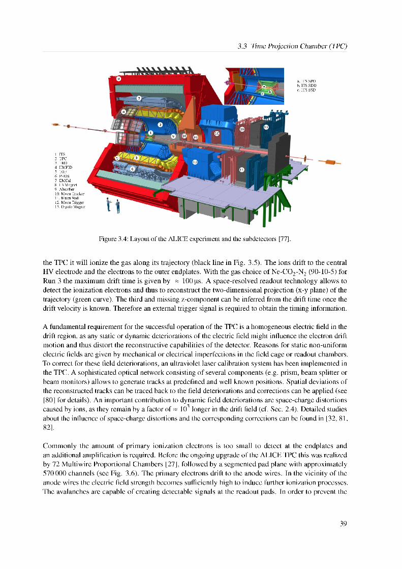
3.3 Time Projection Chamber (TPC)
1. ITS2. TPC3. TRD4. HMPID5. TOF6. PHOS7. EMCal8. L3 Magnet9. Absorber10. Muon Tracker11. MuonWall12. Muon Trigger13. Dipole Magnet
Figure 3.4: Layout of the ALICE experiment and the subdetectors [77].
a. ITS SPDb. ITS SDDc. ITS SSD
the TPC it will ionize the gas along its trajectory (black line in Fig. 3.5). The ions drift to the central HV electrode and the electrons to the outer endplates. With the gas choice of Ne-CO2-N2 (90-10-5) for Run 3 the maximum drift time is given by « 100 ps. A space-resolved readout technology allows to detect the ionization electrons and thus to reconstruct the two-dimensional projection (x-y plane) of the trajectory (green curve). The third and missing z-component can be inferred from the drift time once the drift velocity is known. Therefore an external trigger signal is required to obtain the timing information.
A fundamental requirement for the successful operation of the TPC is a homogeneous electric field in the drift region, as any static or dynamic deteriorations of the electric field might influence the electron drift motion and thus distort the reconstructive capabilities of the detector. Reasons for static non-uniform electric fields are given by mechanical or electrical imperfections in the field cage or readout chambers. To correct for these field deteriorations, an ultraviolet laser calibration system has been implemented in the TPC. A sophisticated optical network consisting of several components (e.g. prism, beam splitter or beam monitors) allows to generate tracks at predefined and well known positions. Spatial deviations of the reconstructed tracks can be traced back to the field deteriorations and corrections can be applied (see [80] for details). An important contribution to dynamic field deteriorations are space-charge distortions caused by ions, as they remain by a factor of « 103 longer in the drift field (cf. Sec. 2.4). Detailed studies about the influence of space-charge distortions and the corresponding corrections can be found in [32, 81, 82].
Commonly the amount of primary ionization electrons is too small to detect at the endplates and an additional amplification is required. Before the ongoing upgrade of the ALICE TPC this was realized by 72 Multiwire Proportional Chambers [27], followed by a segmented pad plane with approximately 570 000 channels (see Fig. 3.6). The primary electrons drift to the anode wires. In the vicinity of the anode wires the electric field strength becomes sufficiently high to induce further ionization processes. The avalanches are capable of creating detectable signals at the readout pads. In order to prevent the
39
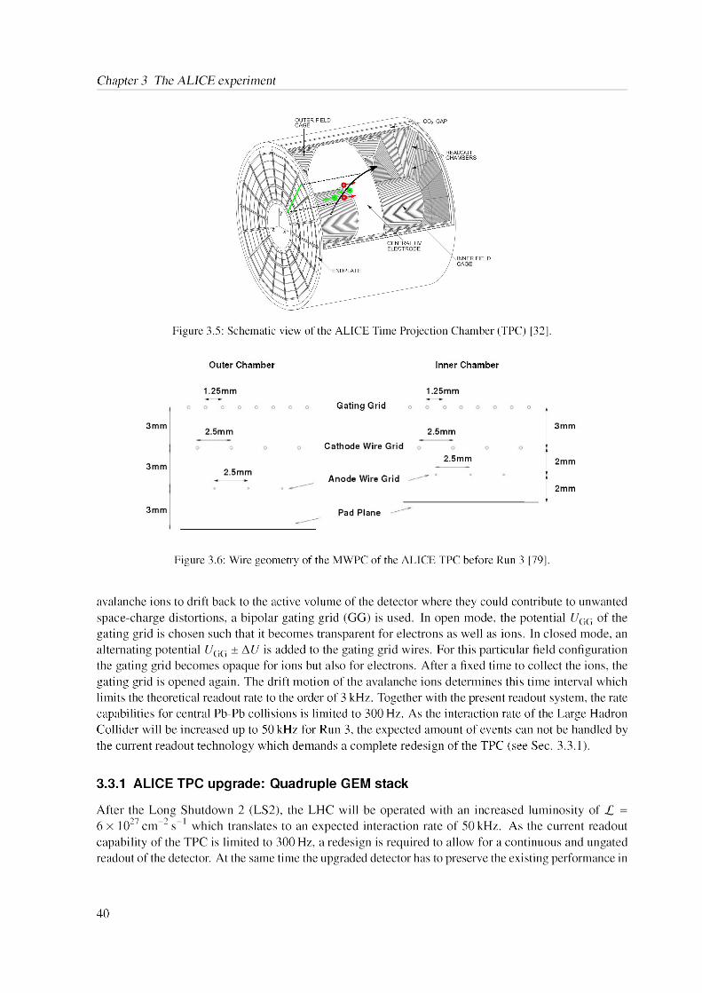
Chapter 3 The ALICE experiment
-C02 GAP
Figure 3.5: Schematic view of the ALICE Time Projection Chamber (TPC) [32].
Outer Chamber Inner Chamber
1.25mm 1.25mmGating Grid
3mm 2.5mm 2.5mm 3mm
Cathode Wire Grid
3mm 2.5mmAnode Wire Grid
2.5mm 2mm
2mm
3mm Pad Plane
Figure 3.6: Wire geometry of the MWPC of the ALICE TPC before Run 3 [79].
avalanche ions to drift back to the active volume of the detector where they could contribute to unwanted space-charge distortions, a bipolar gating grid (GG) is used. In open mode, the potential UGG of the gating grid is chosen such that it becomes transparent for electrons as well as ions. In closed mode, an alternating potential UGG ± AU is added to the gating grid wires. For this particular field configuration the gating grid becomes opaque for ions but also for electrons. After a fixed time to collect the ions, the gating grid is opened again. The drift motion of the avalanche ions determines this time interval which limits the theoretical readout rate to the order of 3 kHz. Together with the present readout system, the rate capabilities for central Pb-Pb collisions is limited to 300 Hz. As the interaction rate of the Large Hadron Collider will be increased up to 50 kHz for Run 3, the expected amount of events can not be handled by the current readout technology which demands a complete redesign of the TPC (see Sec. 3.3.1).
3.3.1 ALICE TPC upgrade: Quadruple GEM stack
After the Long Shutdown 2 (LS2), the LHC will be operated with an increased luminosity of L = 6 x 1027 cm-2 s"1 which translates to an expected interaction rate of 50 kHz. As the current readout capability of the TPC is limited to 300 Hz, a redesign is required to allow for a continuous and ungated readout of the detector. At the same time the upgraded detector has to preserve the existing performance in
40
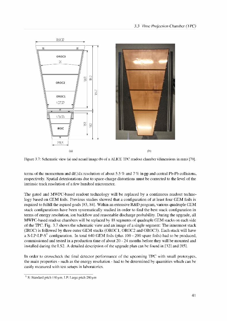
3.3 Time Projection Chamber (TPC)
(a)
Figure 3.7: Schematic view (a) and actual image (b) of a ALICE TPC readout chamber (dimensions in mm) [79].
(b)
terms of the momentum and dE=dx resolution of about 5.5 % and 7 % in pp and central Pb-Pb collisions, respectively. Spatial deteriorations due to space-charge distortions must be corrected to the level of the intrinsic track resolution of a few hundred micrometer.
The gated and MWPC-based readout technology will be replaced by a continuous readout technology based on GEM foils. Previous studies showed that a configuration of at least four GEM foils is required to fulfill the aspired goals [83, 84]. Within an extensive R&D program, various quadruple GEM stack configurations have been systematically studied in order to find the best stack configuration in terms of energy resolution, ion backflow and reasonable discharge probability. During the upgrade, all MWPC-based readout chambers will be replaced by 18 segments of quadruple GEM stacks on each side of the TPC. Fig. 3.7 shows the schematic view and an image of a single segment: The innermost stack (IROC) is followed by three outer GEM stacks (OROC1, OROC2 and OROC3). Each stack will have a S-LP-LP-S1 configuration. In total 640 GEM foils (plus 100 - 200 spare foils) had to be produced, commissioned and tested in a production time of about 20 - 24 months before they will be mounted and installed during the LS2. A detailed description of the upgrade plan can be found in [32] and [85].
1 S: Standard pitch 140 ^m, LP: Large pitch 280 ^m
In order to crosscheck the final detector performance of the upcoming TPC with small prototypes, the main properties - such as the energy resolution - had to be determined by quantities which can be easily measured with test setups in laboratories.
41
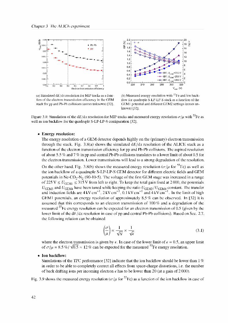
Chapter 3 The ALICE experiment
(a) Simulated AE/Ax resolution for MIP tracks as a function of the electron transmission efficiency in the GEM stack for pp and Pb-Pb collisions (errors unknown) [32].
(b) Measured energy resolution with 55Fe and ion backflow for quadruple S-LP-LP-S stack as a function of the GEM1 potential and different GEM2 settings (errors unknown) [32].
Figure 3.8: Simulation of the dE/dx resolution for MIP tracks and measured energy resolution a/p with 55Fe as well as ion backflow for the quadruple S-LP-LP-S configuration [32].
• Energy resolution:The energy resolution of a GEM detector depends highly on the (primary) electron transmission through the stack. Fig. 3.8(a) shows the simulated dE/dx resolution of the ALICE stack as a function of the electron transmission efficiency for pp and Pb-Pb collisions. The aspired resolution of about 5.5 % and 7 % in pp and central Pb-Pb collisions translates to a lower limit of about 0.5 for the electron transmission. Lower transmissions will lead to a strong degradation of the resolution. On the other hand, Fig. 3.8(b) shows the measured energy resolution (a/p for 55Fe) as well as the ion backflow of a quadruple S-LP-LP-S GEM detector for different electric fields and GEM potentials in Ne-CO2-N2 (90-10-5). The voltage of the first GEM stage was increased in a range of 225 V < CGEM1 < 315 V from left to right. To keep the total gain fixed at 2 000, the potentials CGEM3 and f/GEM4 have been tuned while keeping the ratio f/GEM3 / f/GEM4 constant. The transfer and induction fields are 4 kV cm-1, 2 kV cm-1,0.1 kV cm-1 and 4 kV cm-1. In the limit of high GEM1 potentials, an energy resolution of approximately 8.5 % can be observed. In [32] it is assumed that this corresponds to an electron transmission of 100 % and a degradation of the measured 55Fe energy resolution can be expected for an electron transmission of 0.5 (given by the lower limit of the dE/dx resolution in case of pp and central Pb-Pb collisions). Based on Sec. 2.7, the following relation can be obtained
I j /-^ /p (3.1)
where the electron transmission is given by e. In case of the lower limit of e = 0.5, an upper limit of a/p = 8.5 %/ p05 « 12 % can be expected for the measured 55Fe energy resolution.
• Ion backflow:Simulations of the TPC performance [32] indicate that the ion backflow should be lower than 1 % in order to be able to completely correct all effects from space-charge distortions, i.e. the number of back drifting ions per incoming electron e has to be lower than 20 (at a gain of 2 000).
Fig. 3.9 shows the measured energy resolution (a/p for 55Fe) as a function of the ion backflow in case of
42
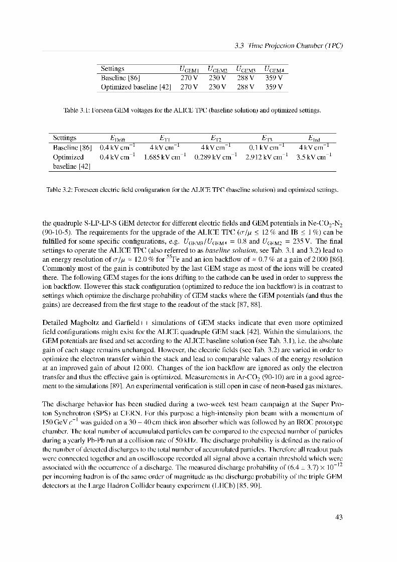
3.3 Time Projection Chamber (TPC)
Table 3.1: Forseen GEM voltages for the ALICE TPC (baseline solution) and optimized settings.
Settings ^GEM1 ^GEM2 ^GEM3 ^GEM4Baseline [86] 270V 230V 288V 359 VOptimized baseline [42] 270V 230V 288V 359 V
Table 3.2: Foreseen electric field configuration for the ALICE TPC (baseline solution) and optimized settings.
Settings EDrift ET1 ET2 ET3 EIndBaseline [86] 0.4kVcm-1 4kV cm-1 4kV cm-1 0.1kVcm-1 4kV cm-1
Optimized baseline [42]
0.4 kV cm-1 1.685 kV cm-1 0.289 kV cm-1 2.912 kV cm-1 3.5 kV cm-1
the quadruple S-LP-LP-S GEM detector for different electric fields and GEM potentials in Ne-CO2-N2 (90-10-5). The requirements for the upgrade of the ALICE TPC (a/p < 12 % and IB < 1 %) can be fulfilled for some specific configurations, e.g. HGEM3/HGEM4 = 0.8 and t/GEM2 = 235 V. The final settings to operate the ALICE TPC (also referred to as baseline solution, see Tab. 3.1 and 3.2) lead to an energy resolution of a/p « 12.0 % for 55Fe and an ion backflow of « 0.7 % at a gain of 2 000 [86]. Commonly most of the gain is contributed by the last GEM stage as most of the ions will be created there. The following GEM stages for the ions drifting to the cathode can be used in order to suppress the ion backflow. However this stack configuration (optimized to reduce the ion backflow) is in contrast to settings which optimize the discharge probability of GEM stacks where the GEM potentials (and thus the gains) are decreased from the first stage to the readout of the stack [87, 88].
Detailed Magboltz and Garfield++ simulations of GEM stacks indicate that even more optimized field configurations might exist for the ALICE quadruple GEM stack [42]. Within the simulations, the GEM potentials are fixed and set according to the ALICE baseline solution (see Tab. 3.1), i.e. the absolute gain of each stage remains unchanged. However, the electric fields (see Tab. 3.2) are varied in order to optimize the electron transfer within the stack and lead to comparable values of the energy resolution at an improved gain of about 12 000. Changes of the ion backflow are ignored as only the electron transfer and thus the effective gain is optimized. Measurements in Ar-CO2 (90-10) are in a good agreement to the simulations [89]. An experimental verification is still open in case of neon-based gas mixtures.
The discharge behavior has been studied during a two-week test beam campaign at the Super Proton Synchrotron (SPS) at CERN. For this purpose a high-intensity pion beam with a momentum of 150 GeV c-1 was guided on a 30 - 40 cm thick iron absorber which was followed by an IROC prototype chamber. The total number of accumulated particles can be compared to the expected number of particles during a yearly Pb-Pb run at a collision rate of 50 kHz. The discharge probability is defined as the ratio of the number of detected discharges to the total number of accumulated particles. Therefore all readout pads were connected together and an oscilloscope recorded all signal above a certain threshold which were
12 associated with the occurrence of a discharge. The measured discharge probability of (6.4 ± 3.7) x 10 per incoming hadron is of the same order of magnitude as the discharge probability of the triple GEM detectors at the Large Hadron Collider beauty experiment (LHCb) [85, 90].
43
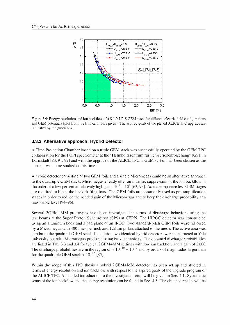
Chapter 3 The ALICE experiment
Figure 3.9: Energy resolution and ion backflow of a S-LP-LP-S GEM stack for different electric field configurations and GEM potentials (plot from [32], no error bars given). The aspired goals of the planed ALICE TPC upgrade are indicated by the green box.
3.3.2 Alternative approach: Hybrid Detector
A Time Projection Chamber based on a triple GEM stack was successfully operated by the GEM TPC collaboration for the FOPI spectrometer at the "Helmholtzzentrum fur Schwerionenforschung" (GSI) in Darmstadt [83, 91, 92] and with the upgrade of the ALICE TPC, a GEM system has been chosen as the concept was more studied at this time.
A hybrid detector consisting of two GEM foils and a single Micromegas could be an alternative approach to the quadruple GEM stack. Micromegas already offer an intrinsic suppression of the ion backflow in the order of a few percent at relatively high gains 103 - 104 [63, 93]. As a consequence less GEM stages are required to block the back drifting ions. The GEM foils are commonly used as pre-amplification stages in order to reduce the needed gain of the Micromegas and to keep the discharge probability at a reasonable level [94-96].
Several 2GEM+MM prototypes have been investigated in terms of discharge behavior during the test beams at the Super Proton Synchrotron (SPS) at CERN. The HIROC detector was constructed using an aluminum body and a pad plane of an IROC. Two standard-pitch GEM foils were followed by a Micromegas with 400 lines per inch and 128 pm pillars attached to the mesh. The active area was similar to the quadruple GEM stack. In addition two identical hybrid detectors were constructed at Yale university but with Micromegas produced using bulk technology. The obtained discharge probabilities are listed in Tab. 3.3 and 3.4 for typical 2GEM+MM settings with low ion backflow and a gain of 2 000. The discharge probabilities are in the region of « 10”10 - 10~9 and by orders of magnitudes larger than for the quadruple GEM stack « 10”12 [85].
Within the scope of this PhD thesis a hybrid 2GEM+MM detector has been set up and studied in terms of energy resolution and ion backflow with respect to the aspired goals of the upgrade program of the ALICE TPC. A detailed introduction to the investigated setup will be given in Sec. 4.1. Systematic scans of the ion backflow and the energy resolution can be found in Sec. 4.3. The obtained results will be
44
3.3 Time Projection Chamber (TPC)
Table 3.3: Discharge probabilities of the HIROC prototype in Ne-CO2-N2 (90-10-5). Field configurations for all settings are EDrift = 390 Van"1, ET1 = 3 875 Van"1 and ET2 = 150 Vcm"1 [85].
UGEM1 / V UGEM2 /V ^MM / V Gain Discharge probability232 210 460 2 000 (3.0 ± 0.3) x 10"9
250 210 440 1800 (3.1 ± 0.7) x 10-10
260 220 420 1 600 (1.5 ± 1.1) x 10-11
Table 3.4: Discharge probabilities of the Yale prototypes in Ne-CO2-N2 (90-10-5). Field configurations of the first two settings are EDrift = 400Vcm-1, ET1 = 3 875 Vcm-1 and ET2 = 90Vcm-1. For the last settings EDrift = 21 Vcm-1, ET1 = 3Vcm-1 and ET2 = 2Vcm-1 [85].
UGEM1 / V UGEM2 /V UMM / V Gain Discharge probability250 210 440 2 050 (2.0 ± 0.6) x 10-9
260 220 420 2 000 (3.5 ± 0.6) x 10-10
0 0 420 450 (1.7 ± 0.5) x 10-10
compared to results of the Yale university in Sec. 4.3.3. Finally the measurements will be compared to dedicated model calculations which will be part of Sec. 6.
45

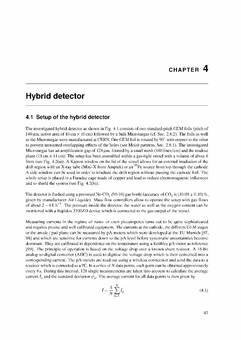
CHAPTER 4
Hybrid detector
4.1 Setup of the hybrid detector
The investigated hybrid detector as shown in Fig. 4.1 consists of two standard-pitch GEM foils (pitch of 140 pm, active area of 10 cm x 10 cm) followed by a bulk Micromegas (cf. Sec. 2.8.2). The foils as well as the Micromegas were manufactured at CERN. One GEM foil is rotated by 90° with respect to the other to prevent unwanted overlapping effects of the holes (see Moire patterns, Sec. 2.8.1). The investigated Micromegas has an amplification gap of 128 pm, formed by a small mesh (160 lines/cm) and the readout plane (11 cm x 11 cm). The setup has been assembled within a gas-tight vessel with a volume of about 6 liters (see Fig. 4.2(a)). A Kapton window on the lid of the vessel allows for an external irradiation of the drift region with an X-ray tube (Mini-X from Amptek) or an 55Fe source from top through the cathode. A side window can be used in order to irradiate the drift region without passing the cathode foil. The whole setup is placed in a Faraday cage made of copper and lead to reduce electromagnetic influences and to shield the system (see Fig. 4.2(b)).
The detector is flushed using a premixed Ne-CO2 (90-10) gas bottle (accuracy of CO2 is (10.09 ± 0.10) %, given by manufacturer Air Liquide). Mass flow controllers allow to operate the setup with gas flows of about 2 - 6 Lh-1. The pressure inside the detector, the water as well as the oxygen content can be monitored with a Rapidox 3100ZD device which is connected to the gas output of the vessel.
Measuring currents in the regime of nano- or even picoamperes turns out to be quite sophisticated and requires precise and well calibrated equipment. The currents at the cathode, the different GEM stages or the anode / pad plane can be measured by pA-meters which were developed at the TU Munich [97, 98] and which are sensitive for currents down to the pA level before systematic uncertainties become dominant. They are calibrated in dependence on the temperature using a Keithley pA-meter as reference [99]. The principle of operation is based on the voltage drop over a known shunt resistor. A 16-bit analog-to-digital converter (ADC) is used to digitize the voltage drop which is then converted into a corresponding current. The pA-meters are read out using a wireless connection and send the data to a receiver which is connected to a PC. In a series of N data points, each point can be obtained approximately every 8 s. During this interval, 128 single measurements are taken into account to calculate the average current In and the standard deviation an. The average current for all data points is then given by
1 X1 = -N Z 4 (4-0
47
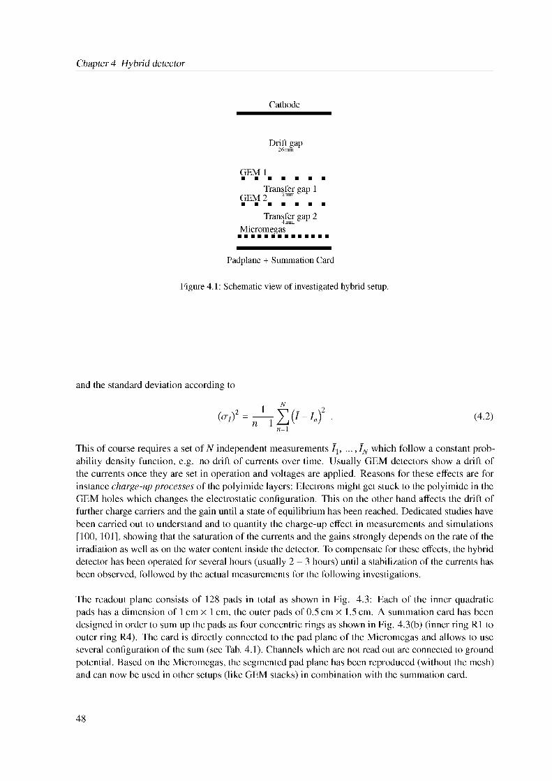
Chapter 4 Hybrid detector
Cathode
Drift gap26mm
GEM 1
Transfer gap 1GEM 2 2mm
Transfer gap 24mm D 1
Micromegas
Padplane + Summation Card
Figure 4.1: Schematic view of investigated hybrid setup.
and the standard deviation according to
' =n', X (I - In)2 • ■■'n 1 -1 n=1
This of course requires a set of N independent measurements Ip ..., IN which follow a constant probability density function, e.g. no drift of currents over time. Usually GEM detectors show a drift of the currents once they are set in operation and voltages are applied. Reasons for these effects are for instance charge-up processes of the polyimide layers: Electrons might get stuck to the polyimide in the GEM holes which changes the electrostatic configuration. This on the other hand affects the drift of further charge carriers and the gain until a state of equilibrium has been reached. Dedicated studies have been carried out to understand and to quantity the charge-up effect in measurements and simulations [100, 101], showing that the saturation of the currents and the gains strongly depends on the rate of the irradiation as well as on the water content inside the detector. To compensate for these effects, the hybrid detector has been operated for several hours (usually 2 - 3 hours) until a stabilization of the currents has been observed, followed by the actual measurements for the following investigations.
The readout plane consists of 128 pads in total as shown in Fig. 4.3: Each of the inner quadratic pads has a dimension of 1 cm x 1 cm, the outer pads of 0.5 cm x 1.5 cm. A summation card has been designed in order to sum up the pads as four concentric rings as shown in Fig. 4.3(b) (inner ring R1 to outer ring R4). The card is directly connected to the pad plane of the Micromegas and allows to use several configuration of the sum (see Tab. 4.1). Channels which are not read out are connected to ground potential. Based on the Micromegas, the segmented pad plane has been reproduced (without the mesh) and can now be used in other setups (like GEM stacks) in combination with the summation card.
48
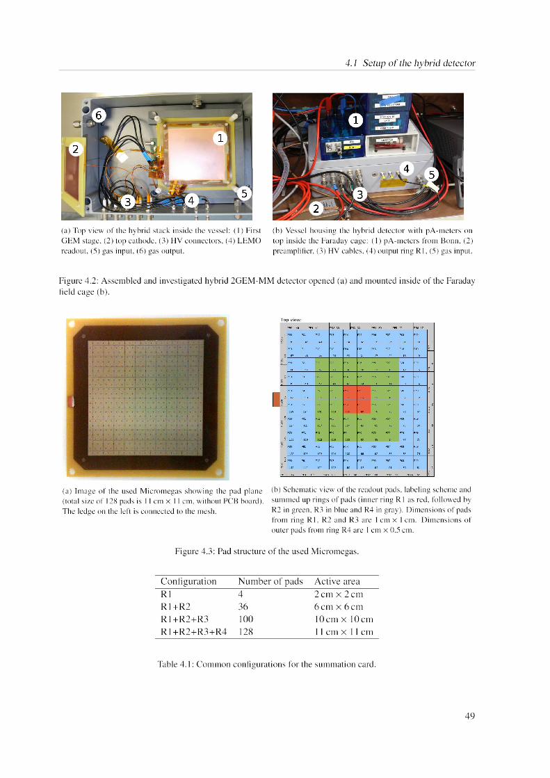
4.1 Setup of the hybrid detector
(a) Top view of the hybrid stack inside the vessel: (1) First GEM stage, (2) top cathode, (3) HV connectors, (4) LEMO readout, (5) gas input, (6) gas output.
(b) Vessel housing the hybrid detector with pA-meters on top inside the Faraday cage: (1) pA-meters from Bonn, (2) preamplifier, (3) HV cables, (4) output ring R1, (5) gas input.
Figure 4.2: Assembled and investigated hybrid 2GEM-MM detector opened (a) and mounted inside of the Faraday field cage (b).
Top view:
(a) Image of the used Micromegas showing the pad plane (total size of 128 pads is 11 cm x 11 cm, without PCB board). The ledge on the left is connected to the mesh.
(b) Schematic view of the readout pads, labeling scheme and summed up rings of pads (inner ring R1 as red, followed by R2 in green, R3 in blue and R4 in gray). Dimensions of pads from ring R1, R2 and R3 are 1 cm x 1 cm. Dimensions of outer pads from ring R4 are 1 cm x 0.5 cm.
Figure 4.3: Pad structure of the used Micromegas.
Table 4.1: Common configurations for the summation card.
Configuration Number of pads Active areaR1 4 2 cm x 2 cmR1+R2 36 6 cm x 6 cmR1+R2+R3 100 10 cm x 10 cmR1+R2+R3+R4 128 11 cm x 11 cm
49
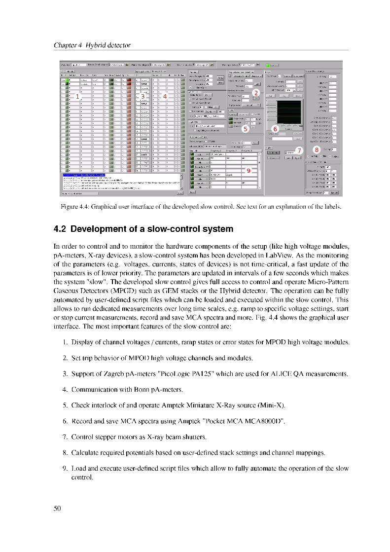
Chapter4 Hybrid detector
Figure 4.4: Graphical user interface of the developed slow control. See text for an explanation of the labels.
4.2 Development of a slow-control system
In order to control and to monitor the hardware components of the setup (like high voltage modules, pA-meters, X-ray devices), a slow-control system has been developed in LabView. As the monitoring of the parameters (e.g. voltages, currents, states of devices) is not time-critical, a fast update of the parameters is of lower priority. The parameters are updated in intervals of a few seconds which makes the system "slow". The developed slow control gives full access to control and operate Micro-Pattern Gaseous Detectors (MPGD) such as GEM stacks or the Hybrid detector. The operation can be fully automated by user-defined script files which can be loaded and executed within the slow control. This allows to run dedicated measurements over long time scales, e.g. ramp to specific voltage settings, start or stop current measurements, record and save MCA spectra and more. Fig. 4.4 shows the graphical user interface. The most important features of the slow control are:
1. Display of channel voltages / currents, ramp states or error states for MPOD high voltage modules.
2. Set trip behavior of MPOD high voltage channels and modules.
3. Support of Zagreb pA-meters "PicoLogic PA125" which are used for ALICE QA measurements.
4. Communication with Bonn pA-meters.
5. Check interlock of and operate Amptek Miniature X-Ray source (Mini-X).
6. Record and save MCA spectra using Amptek "Pocket MCA MCA8000D".
7. Control stepper motors as X-ray beam shutters.
8. Calculate required potentials based on user-defined stack settings and channel mappings.
9. Load and execute user-defined script files which allow to fully automate the operation of the slow control.
50

4.2 Development of a slow-control system
A detailed manual / user guide for the slow control can be found in the appendix A.3. The principle of operation and the technical background will be discussed in the following.
The Slow Control has been developed in LabView 2014 and requires a 32-bit architecture in order to work with the Application Programming Interface (API) of the hardware components (MPOD high voltage modules, Amptek Mini-X and Multichannel Analyzer). The Slow Control has been designed as a three-states machine: Once initialized (state 1), the software idles and allows to configure all relevant operational information (e.g. MPOD controller, pA-meter stations, database connections). By connecting to the MPOD crate (state 2), the Graphical User Interface (GUI) is locked. Once connected (state 3), operational panels are activated and the Slow Control enters the main loop which continuously communicates with the hardware components.
Based on the specific IP and the port of the MPOD controller, an ethernet connection is established to the high voltage crate by using the Simple Network Managment Protocol (SNMP) and the provided Dynamic Link Libraries (DLL) from Wiener. Within the main routine of the Slow Control, the status of each channel and module is polled every half of a second and user commands are sent (e.g. ramping to specific settings or voltages).
The communication with the Mini-X is based on the provided API by Amptek, allowing to access the USB port and thus the X-Ray device. Once connected, the Slow Control checks if a valid session is running and reads out the Serial number of the device. Within an implemented routine, the status registers and the interlock are checked repeatedly. The readout of the Multichannel Analyzer (MCA) uses a specific API by Amptek which allows to make use of the serial port for data transfer. Here a RS232-USB converter has been used in order to connect the MCA to the USB port instead of the serial port.
The operation of the pA-meters from Bonn is based on a pSQL1 database (cf. Fig. 4.5). All relevant information of the pA-meters (mean value, error value, mode of operation, battery state, station id and timestamp) are continuously sent to the readout PC via bluetooth and stored to a database as long as the continue flag (CFlag) of a specific device is activated. The Slow Control is capable of reading out the database in order to fetch the requested data. In addition, the continue flag can be set for each specific device, which is then polled by the readout system. The usage of an ethernet connection between the readout system (blue), the pSQL server (gray) and the Slow Control (green) allows remote operation and to run several pA-meters at different places simultaneously.
1 https://www.postgresql.org2 http://www.picologic.hr
With the upgrade of the ALICE Time Projection Chamber and the Quality Assurance (QA) program developed in this context, a communication with the pA-meters manufactured in Zagreb2 (PicoLogic PA125) had to be implemented as well. These pA-meters are optically linked to a common FPGA board which is thereupon connected to a readout PC (see Fig. 4.6). A further LabView program stores the recorded data to the National Instruments Distributed System Manager (NI-DSM). This server can either run locally (on the same machine) or on a remote system and reached via ethernet. The Slow Control connects to this server and obtains the data of the pA-meters. Again, a spatial separation can be realized using ethernet connections.
51
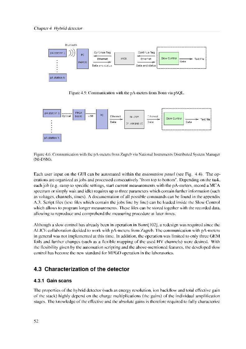
Chapter 4 Hybrid detector
Data and status
Ethernet
Continue flag
pSQL
Continue flag |
Ethernet Slow ControlData
Text file i
Figure 4.5: Communication with the pA-meters from Bonn via pSQL.
Ethernet
Data
NI-DSM
(ni.var.psp://)
Ethernet
DataSlow Control
DataText file j
Figure 4.6: Communication with the pA-meters from Zagreb via National Instruments Distributed System Manager (NI-DSM).
Each user input on the GUI can be automated within the automation panel (see Fig. 4.4). The operations are organized as jobs and processed consecutively "from top to bottom". Depending on the task, each job (e.g. ramp to specific settings, start current measurements with the pA-meters, record a MCA spectrum or simply wait and idle) requires up to three parameters which contain further information (such as voltages, channels, times). A documentation of all possible commands can be found in the appendix A.3. Script files (text files which contain the jobs line by line) can be loaded inside the Slow Control which allows to program longer measurements. These files can be stored together with the recorded data, allowing to reproduce and comprehend the measuring procedure at later times.
Although a slow control has already been in operation in Bonn[102], a redesign was required since the ALICE collaboration decided to work with pA-meters from Zagreb. The communication with pA-meters in general was not implemented at this time. In addition, the operation was limited to only three GEM foils and further changes (such as a flexible mapping of the used HV channels) were desired. With the flexibility given by the automation scripting and the above-mentioned features, the developed slow control has become the new standard for MPGD operation in the laboratories.
4.3 Characterization of the detector
4.3.1 Gain scans
The properties of the hybrid detector (such as energy resolution, ion backflow and total effective gain of the stack) highly depend on the charge multiplications (the gains) of the individual amplification stages. The knowledge of the effective and the absolute gains is therefore required to fully characterize
52
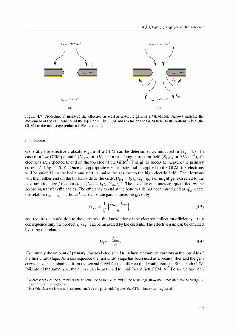
4.3 Characterization of the detector
E above = 400Vcm 1
= 0V
Io
Ebelow = V
(a) (b)
Figure 4.7: Procedure to measure the effective as well as absolute gain of a GEM foil. Arrows indicate the movement of the electrons to (a) the top side of the GEM and (b) inside the GEM hole, to the bottom side of the GEM / to the next stage (either a GEM or anode).
the detector.
Generally the effective / absolute gain of a GEM can be determined as indicated in Fig. 4.7: In case of a low GEM potential (^GEM = 0 V) and a vanishing extraction field (Ebelow = 0 Vcm-1), all electrons are expected to end on the top side of the GEM3. This gives access to measure the primary current I0 (Fig. 4.7(a)). Once an appropriate electric potential is applied to the GEM, the electrons will be guided into the holes and start to ionize the gas due to the high electric field. The electrons will then either end on the bottom side of the GEM (Ibot = I0 e- Gabs ebot) or might get extracted to the next amplification / readout stage (Iextr = I0 e- Gabs e-). The possible outcomes are quantified by the according transfer efficiencies. The efficiency to end at the bottom side has been introduced as ebot where the relation ebot + e~ = 1 holds4. The absolute gain is therefore given by
3 A crosscheck of the currents at the bottom side of the GEM and at the next stage show that a possible reach-through of electrons can be neglected.4 Possible electron losses at insulators - such as the polyimide layer of the GEM - have been neglected.
1 Ibot + Iextrabs = — I 7 ■ (4.3)
ec 70
and requires - in addition to the currents - the knowledge of the electron collection efficiency. As a consequence only the product e- Gabs can be measured by the currents. The effective gain can be obtained by using the relation
Geff = ■ (4.4)I0
Commonly the amount of primary charges is too small to induce measurable currents at the top side of the first GEM stage. As a consequence the first GEM stage has been used as a preamplifier and the gain curves have been obtained from the second GEM for the different field configurations. Since both GEM foils are of the same type, the curves can be assumed to hold for the first GEM. A 55Fe source has been
53
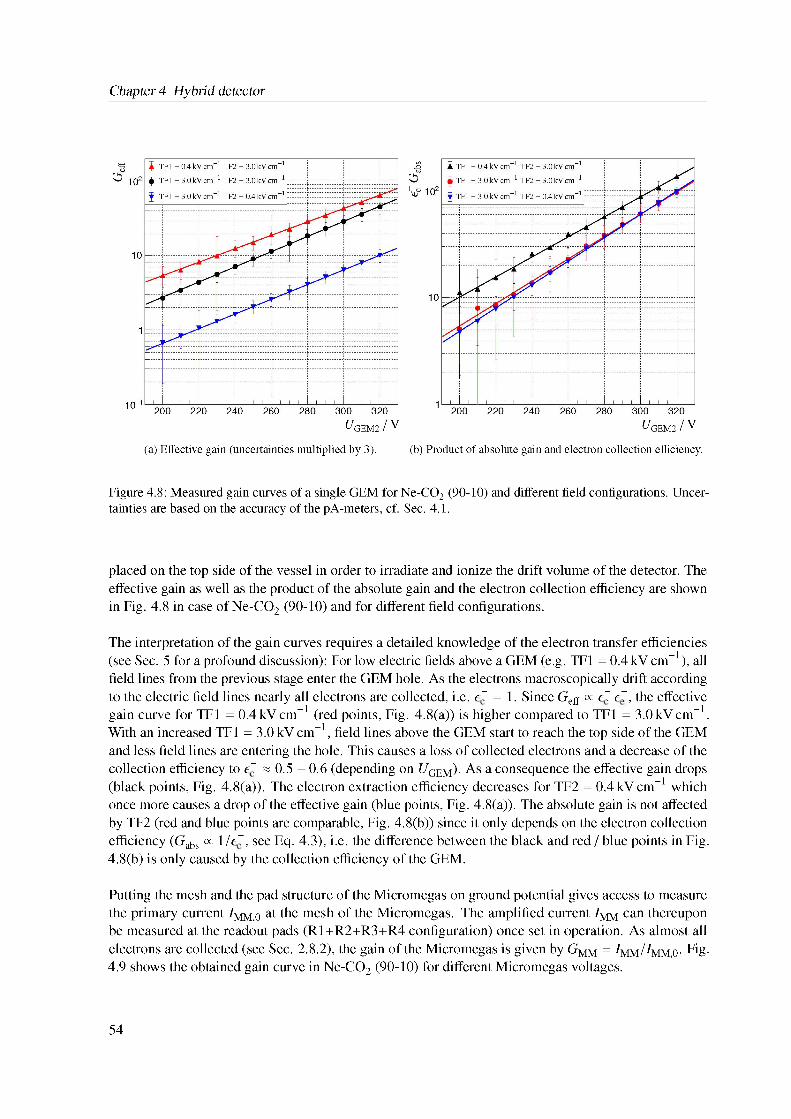
Chapter 4 Hybrid detector
UGEM2 I V
(a) Effective gain (uncertainties multiplied by 3).
UGEM2 I V
(b) Product of absolute gain and electron collection efficiency.
Figure 4.8: Measured gain curves of a single GEM for Ne-CO2 (90-10) and different field configurations. Uncertainties are based on the accuracy of the pA-meters, cf. Sec. 4.1.
placed on the top side of the vessel in order to irradiate and ionize the drift volume of the detector. The effective gain as well as the product of the absolute gain and the electron collection efficiency are shown in Fig. 4.8 in case of Ne-CO2 (90-10) and for different field configurations.
The interpretation of the gain curves requires a detailed knowledge of the electron transfer efficiencies (see Sec. 5 for a profound discussion): For low electric fields above a GEM (e.g. TF1 = 0.4 kV cm-1), all field lines from the previous stage enter the GEM hole. As the electrons macroscopically drift according to the electric field lines nearly all electrons are collected, i.e. e~ = 1. Since Geff / e~ e~, the effective gain curve for TF1 = 0.4 kV cm-1 (red points, Fig. 4.8(a)) is higher compared to TF1 = 3.0 kV cm-1. With an increased TF1 = 3.0 kV cm-1, field lines above the GEM start to reach the top side of the GEM and less field lines are entering the hole. This causes a loss of collected electrons and a decrease of the collection efficiency to e~ & 0.5 - 0.6 (depending on UGEM). As a consequence the effective gain drops (black points, Fig. 4.8(a)). The electron extraction efficiency decreases for TF2 = 0.4 kV cm-1 which once more causes a drop of the effective gain (blue points, Fig. 4.8(a)). The absolute gain is not affected by TF2 (red and blue points are comparable, Fig. 4.8(b)) since it only depends on the electron collection efficiency (Gabs / 1 /e~, see Eq. 4.3), i.e. the difference between the black and red I blue points in Fig. 4.8(b) is only caused by the collection efficiency of the GEM.
Putting the mesh and the pad structure of the Micromegas on ground potential gives access to measure the primary current IMM;0 at the mesh of the Micromegas. The amplified current IMM can thereupon be measured at the readout pads (R1+R2+R3+R4 configuration) once set in operation. As almost all electrons are collected (see Sec. 2.8.2), the gain of the Micromegas is given by GMM = IMM/IMM;0. Fig.4.9 shows the obtained gain curve in Ne-CO2 (90-10) for different Micromegas voltages.
54
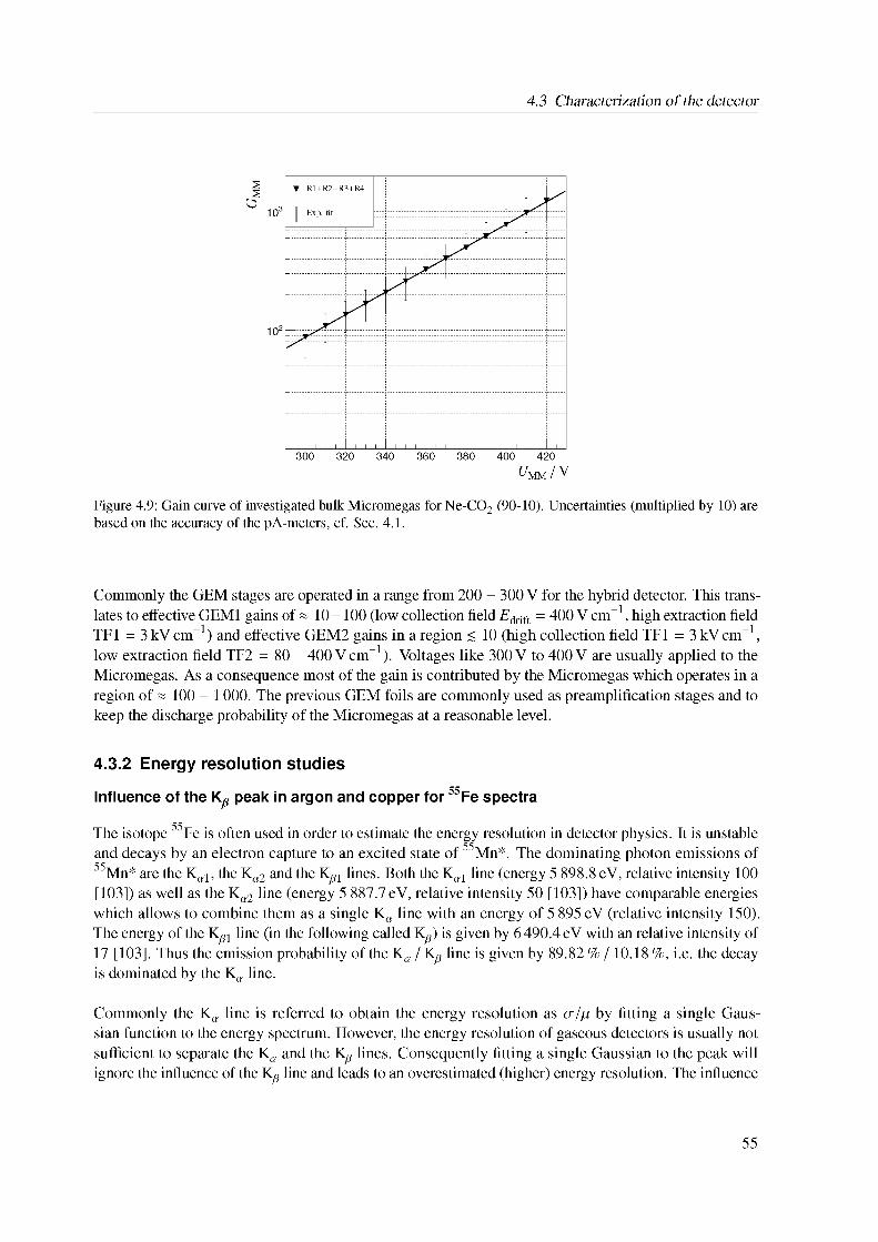
4.3 Characterization of the detector
Figure 4.9: Gain curve of investigated bulk Micromegas for Ne-CO2 (90-10). Uncertainties (multiplied by 10) are based on the accuracy of the pA-meters, cf. Sec. 4.1.
Commonly the GEM stages are operated in a range from 200 - 300 V for the hybrid detector. This translates to effective GEM1 gains of « 10 -100 (low collection field Edrift = 400 V cm-1, high extraction field TF1 = 3 kV cm-1) and effective GEM2 gains in a region < 10 (high collection field TF1 = 3 kV cm-1, low extraction field TF2 = 80 - 400 V cm-1). Voltages like 300 V to 400 V are usually applied to the Micromegas. As a consequence most of the gain is contributed by the Micromegas which operates in a region of « 100 - 1 000. The previous GEM foils are commonly used as preamplification stages and to keep the discharge probability of the Micromegas at a reasonable level.
4.3.2 Energy resolution studiesInfluence of the Kg peak in argon and copper for 55Fe spectra
The isotope 55Fe is often used in order to estimate the energy resolution in detector physics. It is unstable and decays by an electron capture to an excited state of 55Mn*. The dominating photon emissions of 55Mn* are the Ka1, the Ka2 and the Kg1 lines. Both the Ka1 line (energy 5 898.8 eV, relative intensity 100 [103]) as well as the K((,2 line (energy 5 887.7 eV, relative intensity 50 [103]) have comparable energies which allows to combine them as a single Ka line with an energy of 5 895 eV (relative intensity 150). The energy of the Kg1 line (in the following called Kg) is given by 6 490.4 eV with an relative intensity of 17 [103]. Thus the emission probability of the Ka / Kg line is given by 89.82 % / 10.18 %, i.e. the decay is dominated by the Ka line.
Commonly the K((. line is referred to obtain the energy resolution as <r/p by fitting a single Gaussian function to the energy spectrum. However, the energy resolution of gaseous detectors is usually not sufficient to separate the Ka and the Kg lines. Consequently fitting a single Gaussian to the peak will ignore the influence of the Kg line and leads to an overestimated (higher) energy resolution. The influence
55
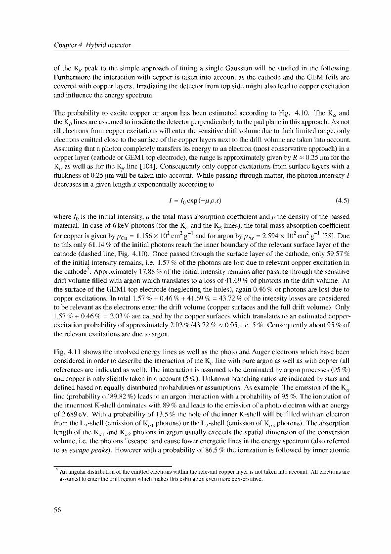
Chapter 4 Hybrid detector
of the Kp peak to the simple approach of fitting a single Gaussian will be studied in the following. Furthermore the interaction with copper is taken into account as the cathode and the GEM foils are covered with copper layers. Irradiating the detector from top side might also lead to copper excitation and influence the energy spectrum.
The probability to excite copper or argon has been estimated according to Fig. 4.10. The K((. and the Kp lines are assumed to irradiate the detector perpendicularly to the pad plane in this approach. As not all electrons from copper excitations will enter the sensitive drift volume due to their limited range, only electrons emitted close to the surface of the copper layers next to the drift volume are taken into account. Assuming that a photon completely transfers its energy to an electron (most conservative approach) in a copper layer (cathode or GEM1 top electrode), the range is approximately given by R & 0.25 pm for the Ka as well as for the Kp line [104]. Consequently only copper excitations from surface layers with a thickness of 0.25 pm will be taken into account. While passing through matter, the photon intensity I decreases in a given length x exponentially according to
I = I0 exp (-p p x) (4.5)
where I0 is the initial intensity, p the total mass absorption coefficient and p the density of the passed material. In case of 6 keV photons (for the Ka and the Kp lines), the total mass absorption coefficient for copper is given by pCu = 1.156 X 102 cm2 g-1 and for argon by pAr = 2.594 X 102 cm2 g-1 [38]. Due to this only 61.14 % of the initial photons reach the inner boundary of the relevant surface layer of the cathode (dashed line, Fig. 4.10). Once passed through the surface layer of the cathode, only 59.57 % of the initial intensity remains, i.e. 1.57 % of the photons are lost due to relevant copper excitation in the cathode5. Approximately 17.88 % of the initial intensity remains after passing through the sensitive drift volume filled with argon which translates to a loss of 41.69 % of photons in the drift volume. At the surface of the GEM1 top electrode (neglecting the holes), again 0.46 % of photons are lost due to copper excitations. In total 1.57 % + 0.46 % + 41.69 % = 43.72 % of the intensity losses are considered to be relevant as the electrons enter the drift volume (copper surfaces and the full drift volume). Only 1.57 % + 0.46 % = 2.03 % are caused by the copper surfaces which translates to an estimated copper- excitation probability of approximately 2.03 %/43.72 % ~ 0.05, i.e. 5 %. Consequently about 95 % of the relevant excitations are due to argon.
5 An angular distribution of the emitted electrons within the relevant copper layer is not taken into account. All electrons are assumed to enter the drift region which makes this estimation even more conservative.
Fig. 4.11 shows the involved energy lines as well as the photo and Auger electrons which have been considered in order to describe the interaction of the K((. line with pure argon as well as with copper (all references are indicated as well). The interaction is assumed to be dominated by argon processes (95 %) and copper is only slightly taken into account (5 %). Unknown branching ratios are indicated by stars and defined based on equally distributed probabilities or assumptions. As example: The emission of the K((. line (probability of 89.82 %) leads to an argon interaction with a probability of 95 %. The ionization of the innermost K-shell dominates with 89 % and leads to the emission of a photo electron with an energy of 2 689 eV. With a probability of 13.5 % the hole of the inner K-shell will be filled with an electron from the L3-shell (emission of Ka1 photons) or the L2-shell (emission of Ka2 photons). The absorption length of the Ka1 and Ka2 photons in argon usually exceeds the spatial dimension of the conversion volume, i.e. the photons "escape" and cause lower energetic lines in the energy spectrum (also referred to as escape peaks). However with a probability of 86.5 % the ionization is followed by inner atomic
56
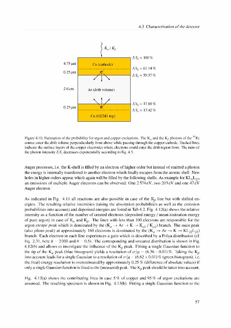
4.3 Characterization of the detector
K / Kg
4.75 pm
0.25 pm
2.6 cm
0.25 pm
Cu (cathode)
e-
Ar (drift volume)
I/I0 - 100 %
I/I0 - 61.14%
I/I0 - 59.57 %
I/I0 - 17.88 %
I/I0 - 17.42 %e
Cu (GEM1 top)
Figure 4.10: Estimation of the probability for argon and copper excitations. The Ka and the Kg photons of the 55Fe source enter the drift volume perpendicularly from above while passing through the copper cathode. Dashed lines indicate the surface layers of the copper electrodes where electrons could enter the drift region from. The ratio of the photon intensity I/I0 decreases exponentially according to Eq. 4.5.
Auger processes, i.e. the K-shell is filled by an electron of higher order but instead of emitted a photon the energy is internally transferred to another electron which finally escapes from the atomic shell. New holes in higher orders appear which again will be filled by the following shells. As example for KL1L23, an emissions of multiple Auger electrons can be observed: One 2 574 eV, two 203 eV and one 47 eV Auger electron.
As indicated in Fig. 4.11 all reactions are also possible in case of the Kg line but with shifted energies. The resulting relative intensities (taking the absorption probabilities as well as the emission probabilities into account) and deposited energies are listed in Tab 4.2. Fig. 4.12(a) shows the relative intensity as a function of the number of created electrons (deposited energy / mean ionization energy of pure argon) in case of Ka and Kg. The lines with less than 100 electrons are responsible for the argon escape peak which is dominated by the (Ka ! Ar ! K ! Ka1 / Ka2) branch. The main peak (also photo peak) at approximately 160 electrons is dominated by the (Ka ! Ar ! K ! KL23L23) branch. Each electron in each line experiences a gain which is described by a Polya distribution (cf. Eq. 2.31, here n = 2000 and Q = 0.5). The corresponding and smeared distribution is shown in Fig. 4.12(b) and allows to investigate the influence of the Kg peak. Fitting a single Gaussian function to the tip of the Ka peak (blue histogram) yields a resolution of a/p = (6.36 ± 0.01) %. Taking the Kg into account leads for a single Gaussian to a resolution of a/p = (6.62 ± 0.01) % (green histogram), i.e. the (real) energy resolution is overestimated by approximately 0.25 % (difference of absolute values) if only a single Gaussian function is fitted to the (measured) peak. The Kg peak should be taken into account.
Fig. 4.13(a) shows the contributing lines in case 5 % of copper and 95 % of argon excitations are assumed. The resulting spectrum is shown in Fig. 4.13(b). Fitting a single Gaussian function to the
57
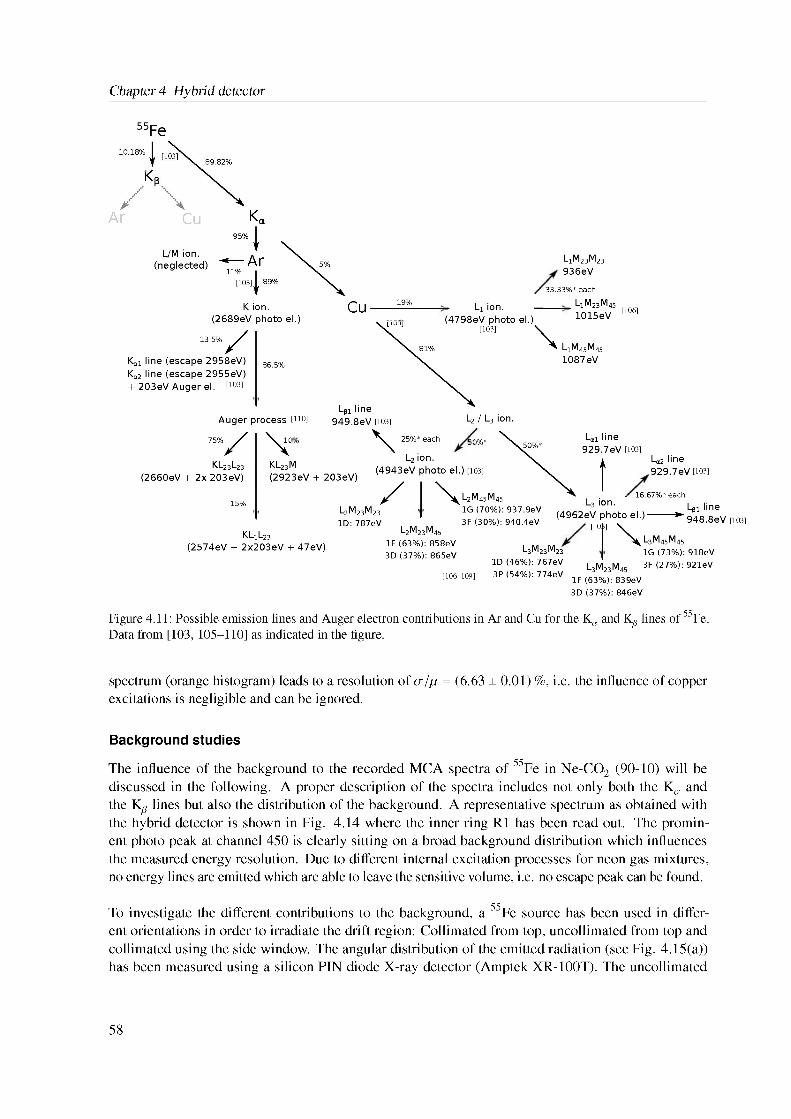
Chapter 4 Hybrid detector
10.18%89.82%
55Fe
Ar Cu
L/M ion. (neglected)
Ka
[103]
K ion.(2689eV photo el.)
L1M23M23
936eV
Cu
13.5%
Ka1 line (escape 2958eV) Ka2 line (escape 2955eV)+ 203eV Auger el. [103]
86.5%
Auger process [110] Lp1 line 949.8eV [103]
19% L1 ion. .(4798eV photo el.)
[103]
33.33%* each
L1M23M45
~1015eV [106]L1M45M45
1087eV
L2 / L3 ion.
75% 25%* each
KL23L23
(2660eV + 2x 203eV)
15%
KL23M
(2923eV + 203eV)
L2M23M231D:787eV
50%*
L2 ion.(4943eV photo el.) [103]
50%* L„1 line 929.7eV [103]
L„2 line 929.7eV [103]
KL1L23
(2574eV + 2x203eV + 47eV)
L2M23M45
1F (63%): 858eV3D (37%): 865eV
L2M45M45
1G (70%): 937.9eV3F (30%): 940.4eV
. 16.67%* eachL3 ion' Lb1 line
(4962eV photo el.)-------- *948.8eV [103][103]
[106-109]
L3M23M23
1D (46%): 767eV3P (54%): 774eV
L3M45M45
1G (73%): 918eVL3M23M45 3F (27%): 921eV
1F (63%): 839eV3D (37%): 846eV
Figure 4.11: Possible emission lines and Auger electron contributions in Ar and Cu for the Ka and Kg lines of 55Fe. Data from [103, 105-110] as indicated in the figure.
spectrum (orange histogram) leads to a resolution of a/p = (6.63 ± 0.01) %, i.e. the influence of copper excitations is negligible and can be ignored.
Background studies
The influence of the background to the recorded MCA spectra of 55Fe in Ne-CO2 (90-10) will be discussed in the following. A proper description of the spectra includes not only both the Ka and the Kg lines but also the distribution of the background. A representative spectrum as obtained with the hybrid detector is shown in Fig. 4.14 where the inner ring R1 has been read out. The prominent photo peak at channel 450 is clearly sitting on a broad background distribution which influences the measured energy resolution. Due to different internal excitation processes for neon gas mixtures, no energy lines are emitted which are able to leave the sensitive volume, i.e. no escape peak can be found.
To investigate the different contributions to the background, a 55Fe source has been used in different orientations in order to irradiate the drift region: Collimated from top, uncollimated from top and collimated using the side window. The angular distribution of the emitted radiation (see Fig. 4.15(a)) has been measured using a silicon PIN diode X-ray detector (Amptek XR-100T). The uncollimated
58
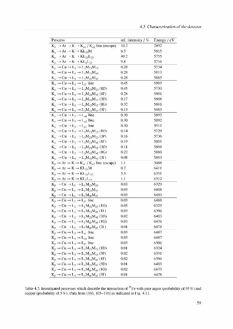
4.3 Characterization of the detector
Table 4.2: Investigated processes which describe the interaction of 55Fe with pure argon (probability of 95 %) and copper (probability of 5 %). Data from [103, 105-110] as indicated in Fig. 4.11.
Process rel. intensity / % Energy / eVK, ! Ar ! K ! K,1 / K,2 line (escape) 10.2 2892K, ! Ar ! K ! KL23M 6.5 5815K, ! Ar ! K ! KL23L23 49.2 5755K, ! Ar ! K ! KL1L23 9.8 5716K, ! Cu ! L1 ! L1M23M23 0.28 5734K, ! Cu ! L1 ! L1M23M45 0.28 5813K, ! Cu ! L1 ! L1M45M45 0.28 5885K, ! Cu ! L2 ! Lg1 line 0.45 5893K , ! Cu ! L2 ! L2M23M23 (1D) 0.45 5730K , ! Cu ! L2 ! L2M23M45 (1F) 0.28 5801K, ! Cu ! L2 ! L2M23M45 (3D) 0.17 5808K, ! Cu ! L2 ! L2M45M45 (1G) 0.32 5881K, ! Cu ! L2 ! L2M45M45 (3F) 0.13 5883K, ! Cu ! L3 ! L,1 line 0.30 5892K , ! Cu ! L3 ! L,2 line 0.30 5892K, ! Cu ! L3 ! Lg1 line 0.30 5911K, ! Cu ! L3 ! L3M23M23 (1D) 0.14 5729K, ! Cu ! L3 ! L3M23M23 (3P) 0.16 5736K, ! Cu ! L3 ! L3M23M45 (1F) 0.19 5801K, ! Cu ! L3 ! L3M23M45 (3D) 0.11 5808K, ! Cu ! L3 ! L3M45M45 (1G) 0.22 5880K, ! Cu ! L3 ! L3M45M45 (3F) 0.08 5883Kg ! Ar ! K ! K,1 / K,2 line (escape) 1.1 3488Kg ! Ar ! K ! KL23M 0.7 6411Kg ! Ar ! K ! KL23L23 5.5 6351K ! Ar ! K ! KL1L23 1.1 6312Kg ! Cu ! L1 ! L1M23M23 0.03 6329Kg ! Cu ! L1 ! L1M23M45 0.03 6408Kg ! Cu ! L1 ! L1M45M45 0.03 6480K^ ! Cu ! L2 ! Lg1 line 0.05 6488Kg ! Cu ! L2 ! L2M23M23 (1D) 0.05 6325Kg ! Cu ! L2 ! L2M23M45 (1F) 0.03 6396Kg ! Cu ! L2 ! L2M23M45 (3D) 0.02 6403Kg ! Cu ! L2 ! L2M45M45 (1G) 0.03 6476Kg ! Cu ! L2 ! L2M45M45 (3F) 0.01 6478K^ ! Cu ! L3 ! L,1 line 0.03 6487Kg ! Cu ! L3 ! L,2 line 0.03 6487K^ ! Cu ! L3 ! Lg1 line 0.03 6506Kg ! Cu ! L3 ! L3M23M23 (1D) 0.01 6324Kg ! Cu ! L3 ! L3M23M23 (3P) 0.02 6331Kg ! Cu ! L3 ! L3M23M45 (1F) 0.02 6396Kg ! Cu ! L3 ! L3M23M45 (3D) 0.01 6403Kg ! Cu ! L3 ! L3M45M45 (1G) 0.02 6475Kg ! Cu ! L3 ! L3M45M45 (3F) 0.01 6478
59
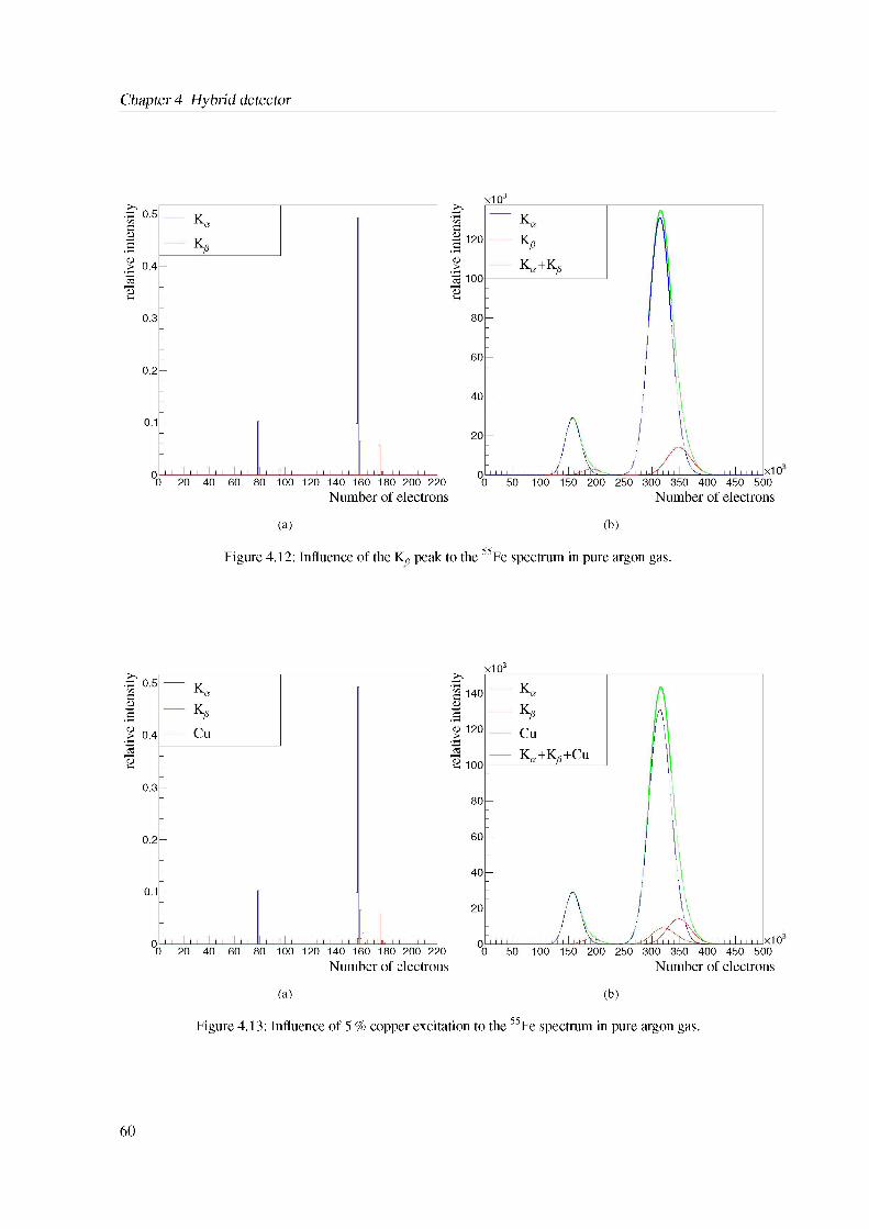
Chapter 4 Hybrid detector
rela
tive i
nten
sity
rela
tive i
nten
sity
Number of electrons
(a) (b)
Figure 4.12: Influence of the Kg peak to the 55Fe spectrum in pure argon gas.
Number of electrons
(a) (b)
Figure 4.13: Influence of 5 % copper excitation to the 55Fe spectrum in pure argon gas.
60
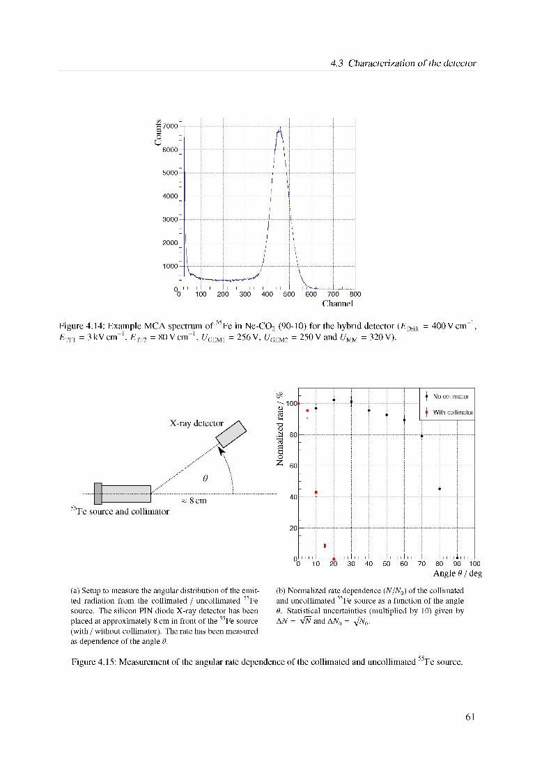
4.3 Characterization of the detector
Figure 4.14: Example MCA spectrum of 55Fe in Ne-CO2 (90-10) for the hybrid detector (EDrift = 400 Vcm 1, Etf1 = 3kVcm ', ETF2 = 80Vcm ', UGEM1 = 256 V, UGEM2 = 250 V and UMM = 320 V).
55
Angle 0 / deg
(a) Setup to measure the angular distribution of the emitted radiation from the collimated / uncollimated 55Fe source. The silicon PIN diode X-ray detector has been placed at approximately 8 cm in front of the 55Fe source (with / without collimator). The rate has been measured as dependence of the angle 0.
(b) Normalized rate dependence (N=N0) of the collimated and uncollimated 55Fe source as a function of the angle 0. Statistical uncertainties (multiplied by 10) given by AN = pN and AN0 = pN0.
Figure 4.15: Measurement of the angular rate dependence of the collimated and uncollimated 55Fe source.
61
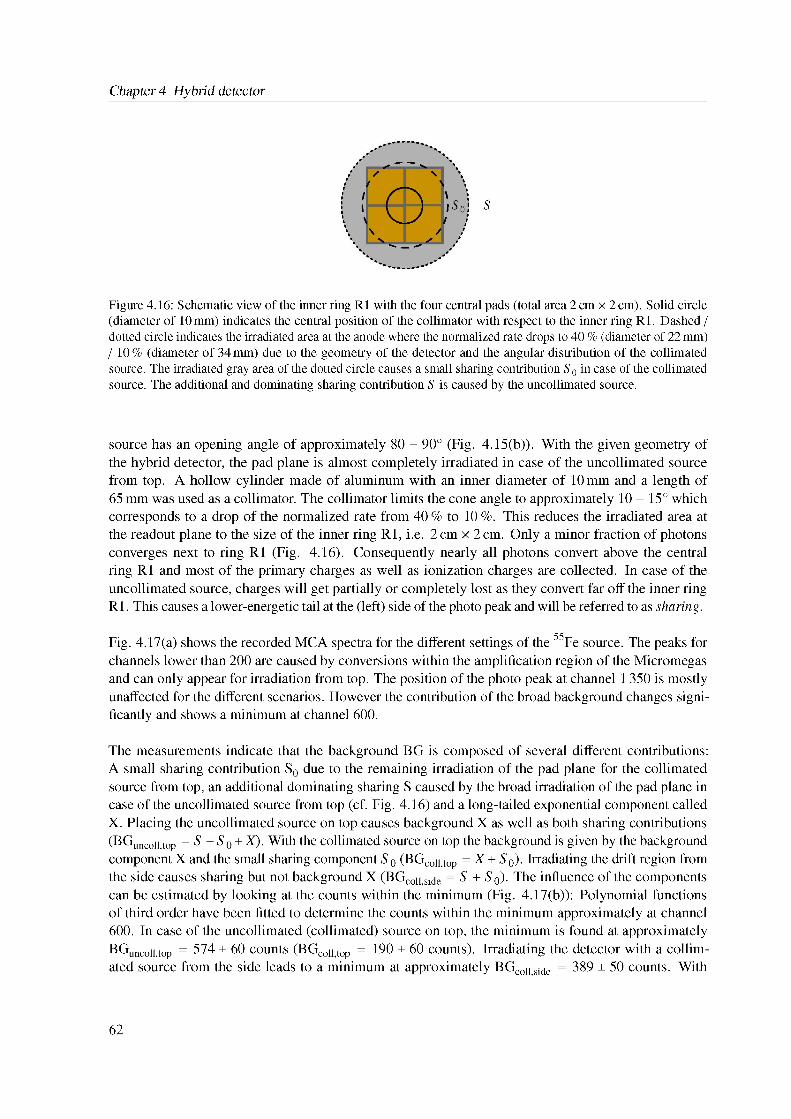
Chapter 4 Hybrid detector
Figure 4.16: Schematic view of the inner ring R1 with the four central pads (total area 2 cm x 2 cm). Solid circle (diameter of 10 mm) indicates the central position of the collimator with respect to the inner ring R1. Dashed / dotted circle indicates the irradiated area at the anode where the normalized rate drops to 40 % (diameter of 22 mm) / 10 % (diameter of 34 mm) due to the geometry of the detector and the angular distribution of the collimated source. The irradiated gray area of the dotted circle causes a small sharing contribution S 0 in case of the collimated source. The additional and dominating sharing contribution S is caused by the uncollimated source.
source has an opening angle of approximately 80 - 90° (Fig. 4.15(b)). With the given geometry of the hybrid detector, the pad plane is almost completely irradiated in case of the uncollimated source from top. A hollow cylinder made of aluminum with an inner diameter of 10 mm and a length of 65 mm was used as a collimator. The collimator limits the cone angle to approximately 10 - 15° which corresponds to a drop of the normalized rate from 40 % to 10 %. This reduces the irradiated area at the readout plane to the size of the inner ring R1, i.e. 2 cm x 2 cm. Only a minor fraction of photons converges next to ring R1 (Fig. 4.16). Consequently nearly all photons convert above the central ring R1 and most of the primary charges as well as ionization charges are collected. In case of the uncollimated source, charges will get partially or completely lost as they convert far off the inner ring R1. This causes a lower-energetic tail at the (left) side of the photo peak and will be referred to as sharing.
Fig. 4.17(a) shows the recorded MCA spectra for the different settings of the 55Fe source. The peaks for channels lower than 200 are caused by conversions within the amplification region of the Micromegas and can only appear for irradiation from top. The position of the photo peak at channel 1 350 is mostly unaffected for the different scenarios. However the contribution of the broad background changes significantly and shows a minimum at channel 600.
The measurements indicate that the background BG is composed of several different contributions: A small sharing contribution S0 due to the remaining irradiation of the pad plane for the collimated source from top, an additional dominating sharing S caused by the broad irradiation of the pad plane in case of the uncollimated source from top (cf. Fig. 4.16) and a long-tailed exponential component called X. Placing the uncollimated source on top causes background X as well as both sharing contributions (BGuncoll;top = S + S 0 + X). With the collimated source on top the background is given by the background component X and the small sharing component S 0 (BGcoll;top = X + S0). Irradiating the drift region from the side causes sharing but not background X (BGcoll;side = S + S 0). The influence of the components can be estimated by looking at the counts within the minimum (Fig. 4.17(b)): Polynomial functions of third order have been fitted to determine the counts within the minimum approximately at channel 600. In case of the uncollimated (collimated) source on top, the minimum is found at approximately BGuncoll;top = 574 ± 60 counts (BGcoll;top = 190 ± 60 counts). Irradiating the detector with a collimated source from the side leads to a minimum at approximately BGcoll;side = 389 ± 50 counts. With
62
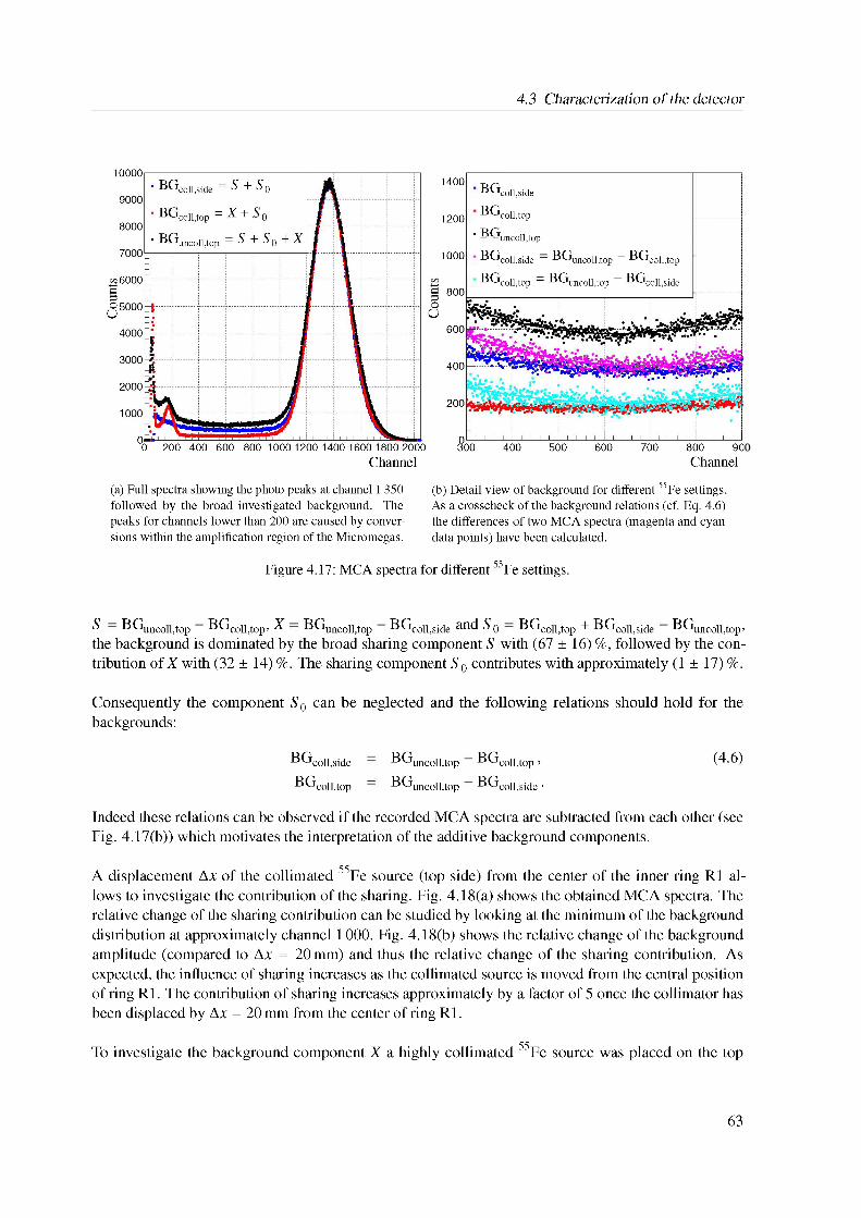
4.3 Characterization of the detector
1400
1200
1000
800
Channel
(a) Full spectra showing the photo peaks at channel 1 350 followed by the broad investigated background. The peaks for channels lower than 200 are caused by conversions within the amplification region of the Micromegas.
BGcoll.side
BGcoll,top. BG .. .uncoll,topBGcoll,side = BGuncoll,top — BGcoll,top
BGcoll,top = BGuncoll,top — BGcoll,side
400
200
600
Channel
(b) Detail view of background for different 55Fe settings. As a crosscheck of the background relations (cf. Eq. 4.6) the differences of two MCA spectra (magenta and cyan data points) have been calculated.
Figure 4.17: MCA spectra for different 55Fe settings.
S BGuncoll,top BGcoll,top, X BGuncoll,top BGcoll,side and S0 BGcoll,top + BGcoll,side BGuncoll,top, the background is dominated by the broad sharing component S with (67 ± 16) %, followed by the contribution of X with (32 ± 14) %. The sharing component S0 contributes with approximately (1 ± 17) %.
Consequently the component S 0 can be neglected and the following relations should hold for the backgrounds:
BGcoll,side BGuncoll,top BGcoll,top , (4.6)
BGcoll,top BGuncoll,top BGcoll,side •
Indeed these relations can be observed if the recorded MCA spectra are subtracted from each other (see Fig. 4.17(b)) which motivates the interpretation of the additive background components.
A displacement Ax of the collimated 55Fe source (top side) from the center of the inner ring R1 allows to investigate the contribution of the sharing. Fig. 4.18(a) shows the obtained MCA spectra. The relative change of the sharing contribution can be studied by looking at the minimum of the background distribution at approximately channel 1 000. Fig. 4.18(b) shows the relative change of the background amplitude (compared to Ax = 20 mm) and thus the relative change of the sharing contribution. As expected, the influence of sharing increases as the collimated source is moved from the central position of ring R1. The contribution of sharing increases approximately by a factor of 5 once the collimator has been displaced by Ax = 20 mm from the center of ring R1.
To investigate the background component X a highly collimated 55Fe source was placed on the top
63
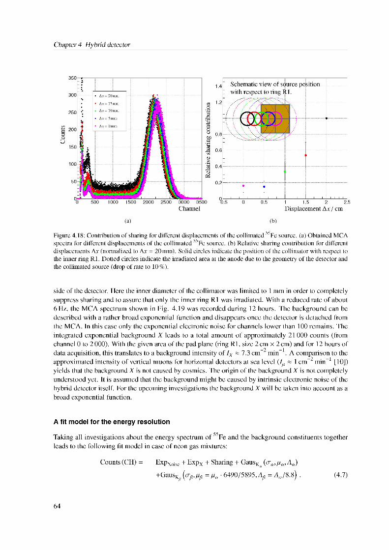
Chapter 4 Hybrid detector
(a) (b)
Figure 4.18: Contribution of sharing for different displacements of the collimated 55Fe source. (a) Obtained MCA spectra for different displacements of the collimated 55Fe source. (b) Relative sharing contribution for different displacements Ax (normalized to Ax = 20 mm). Solid circles indicate the position of the collimator with respect to the inner ring R1. Dotted circles indicate the irradiated area at the anode due to the geometry of the detector and the collimated source (drop of rate to 10 %).
side of the detector. Here the inner diameter of the collimator was limited to 1 mm in order to completely suppress sharing and to assure that only the inner ring R1 was irradiated. With a reduced rate of about 6 Hz, the MCA spectrum shown in Fig. 4.19 was recorded during 12 hours. The background can be described with a rather broad exponential function and disappears once the detector is detached from the MCA. In this case only the exponential electronic noise for channels lower than 100 remains. The integrated exponential background X leads to a total amount of approximately 21000 counts (from channel 0 to 2 000). With the given area of the pad plane (ring R1, size 2 cm X 2 cm) and for 12 hours of data acquisition, this translates to a background intensity of IX « 7.3 cm-2 min-1. A comparison to the approximated intensity of vertical muons for horizontal detectors at sea level (I^ « 1 cm-2 min-1 [10]) yields that the background X is not caused by cosmics. The origin of the background X is not completely understood yet. It is assumed that the background might be caused by intrinsic electronic noise of the hybrid detector itself. For the upcoming investigations the background X will be taken into account as a broad exponential function.
A fit model for the energy resolution
Taking all investigations about the energy spectrum of 55Fe and the background constituents together leads to the following fit model in case of neon gas mixtures:
Counts (CH) = ExpNoise + Expx + Sharing + GausKa (<Ta,Pa, Aa) +Gaus^ (&p,Pp = Pa ' 6490/5895, Ap = Aa/8.8) . (4.7)
64
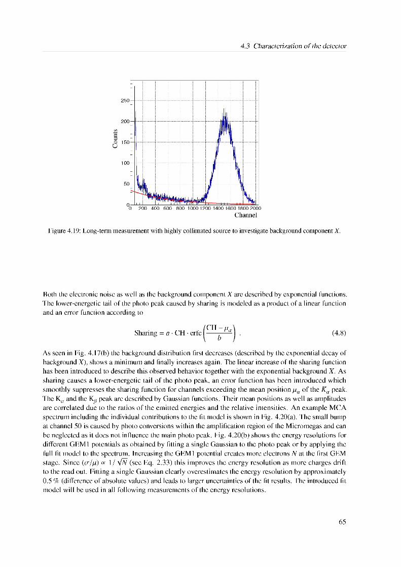
4.3 Characterization of the detector
Channel
Figure 4.19: Long-term measurement with highly collimated source to investigate background component X.
Both the electronic noise as well as the background component X are described by exponential functions. The lower-energetic tail of the photo peak caused by sharing is modeled as a product of a linear function and an error function according to
/CH - pa
\ bSharing = a ■ CH ■ erfc (4.8)
As seen in Fig. 4.17(b) the background distribution first decreases (described by the exponential decay of background X), shows a minimum and finally increases again. The linear increase of the sharing function has been introduced to describe this observed behavior together with the exponential background X. As sharing causes a lower-energetic tail of the photo peak, an error function has been introduced which smoothly suppresses the sharing function for channels exceeding the mean position pa of the Ka peak. The Ka and the Kg peak are described by Gaussian functions. Their mean positions as well as amplitudes are correlated due to the ratios of the emitted energies and the relative intensities. An example MCA spectrum including the individual contributions to the fit model is shown in Fig. 4.20(a). The small bump at channel 50 is caused by photo conversions within the amplification region of the Micromegas and can be neglected as it does not influence the main photo peak. Fig. 4.20(b) shows the energy resolutions for different GEM1 potentials as obtained by fitting a single Gaussian to the photo peak or by applying the full fit model to the spectrum. Increasing the GEM1 potential creates more electrons N at the first GEM stage. Since (a/p) / 1 / y[N (see Eq. 2.33) this improves the energy resolution as more charges drift to the read out. Fitting a single Gaussian clearly overestimates the energy resolution by approximately 0.5 % (difference of absolute values) and leads to larger uncertainties of the fit results. The introduced fit model will be used in all following measurements of the energy resolutions.
65
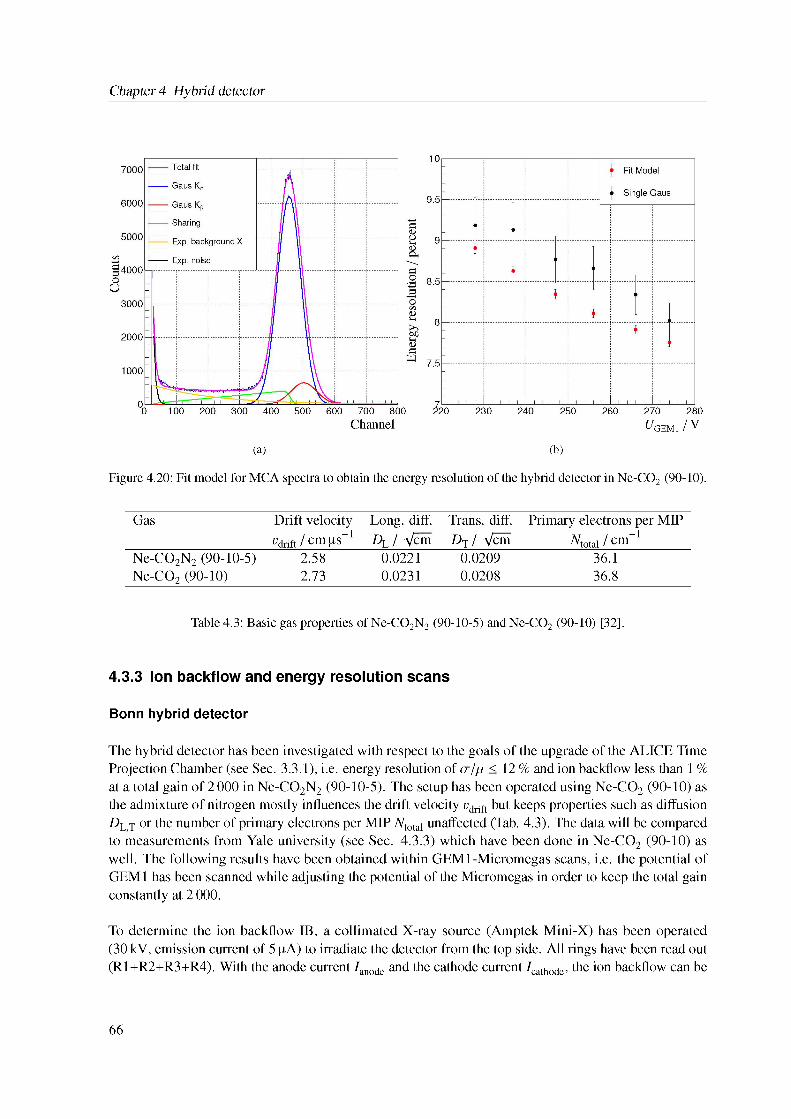
Chapter 4 Hybrid detector
Channel VGEM1 / v
(a) (b)
Figure 4.20: Fit model for MCA spectra to obtain the energy resolution of the hybrid detector in Ne-CO2 (90-10).
Gas Drift velocity Vdrift / cm ^s-1
Long. diff. Dl / Vcm
Trans. diff.Dt / vcm
Primary electrons per MIP Motal / cm-1
Ne-CO2N2 (90-10-5) 2.58 0.0221 0.0209 36.1Ne-CO2 (90-10) 2.73 0.0231 0.0208 36.8
Table 4.3: Basic gas properties of Ne-CO2N2 (90-10-5) andNe-CO2 (90-10) [32].
4.3.3 Ion backflow and energy resolution scans
Bonn hybrid detector
The hybrid detector has been investigated with respect to the goals of the upgrade of the ALICE Time Projection Chamber (see Sec. 3.3.1), i.e. energy resolution of a/p < 12 % and ion backflow less than 1 % at a total gain of 2 000 in Ne-CO2N2 (90-10-5). The setup has been operated using Ne-CO2 (90-10) as the admixture of nitrogen mostly influences the drift velocity vdrift but keeps properties such as diffusion DL;T or the number of primary electrons per MIP Vtotal unaffected (Tab. 4.3). The data will be compared to measurements from Yale university (see Sec. 4.3.3) which have been done in Ne-CO2 (90-10) as well. The following results have been obtained within GEM1-Micromegas scans, i.e. the potential of GEM1 has been scanned while adjusting the potential of the Micromegas in order to keep the total gain constantly at 2 000.
To determine the ion backflow IB, a collimated X-ray source (Amptek Mini-X) has been operated (30 kV, emission current of 5 ^A) to irradiate the detector from the top side. All rings have been read out (R1+R2+R3+R4). With the anode current Zanode and the cathode current Zcathode, the ion backflow can be
66
4.3 Characterization of the detector
obtained by:
IB =| ^cathode |
Ainode(4.9)
The following statistical uncertainties of the ion backflow measurements are determined by the accuracy of the pA-meters, cf. Sec. 4.1.
The total effective gain of the stack has been determined according to Sec. 4.3.1 as the fraction of the current at the readout plane and the initial current within the drift region. Again, the collimated X-ray source has been used to irradiate the full pad plane (R1+R2+R3+R4). Two methods were used in order to measure the primary current: As ions and electrons are created pairwise within the drift region, both the current at the drift cathode Z0,cathode (due to ions) as well as the current at the top side of the first GEM I0,G1T (due to electrons) can be used as initial currents (where | Z0,cathode | ~ I0,G1T). For this purpose all GEM and Micromegas potentials were set to ground and only a drift field of Edrift = 400 V cm-1 has been applied. Since electrons might also convert in the region between GEM2 and the Micromegas (TF2), an offset current Ianode,MMonly has been measured at the readout plane. In this case only the Micromegas has been operated and the according transfer field TF2 has been applied. Conversion between GEM1 and GEM2 has been neglected6 *. Both methods lead to the following effective gains of the stack
6 The procedure has been proposed and used for an alternative hybrid setup of the Yale university [111, 112] and was adoptedto allow for a comparison with the Bonn hybrid detector.
_ Amode — Ianode,MMonly .. .Geff, cathode = TZ | ; (4.10)
| m, cathode |^anode — Ianode,MMonly
Geff,G1T = ------------ T--------------- • (4.11)y0,G1T
Within the GEM1-MM scans, the stack settings have been adjusted in a way to keep the average gain Geff = (Geff, cathode + Geff,G1T) /2 constantly at 2 000. The uncertainties are given by the systematic deviations of both methods to determine the gain as well as the statistical uncertainties of the pA-meter currents.
MCA spectra have been measured using an 55Fe source (rate of about 40 kHz). Only the inner ring R1 was taken into account in order to reduce the dimension (the capacity) of the pad plane and thus to improve the signal-to-noise ratio (SNR). The energy resolution has been calculated using the advanced fit model from Sec. 4.3.2 as well as - for comparison - based on a single Gaussian function. The obtained results are listed in Tab. 4.4 for different values of TF2. The uncertainties of the energy resolutions (a/p) are based on the outcome of the fit results for the mean p ± Ap and the standard deviation a ± Aa (in case of the advanced fit model: mean and sigma of the Ka peak) and obtained by an error propagation according to [A (a/p)]2 = (Aa)2 /p2 + (Ap)2 a2/p4. The environmental conditions (oxygen/water content and overpressure inside the detector, atmospheric pressure, peak temperature of the day as well as relative humidity) during the operation of the setup are listed in Tab. 4.5. As the gain scales with p/T it is an important quantity which influences the ion backflow and the energy resolution [29]. The relative fluctuations of p/T (about 2 %) can be neglected as the environmental conditions and the conditions inside the detector were more or less stable during the period of data acquisition.
Fig. 4.21 shows the measured values of the energy resolution, the ion backflow as well as the gain for
67
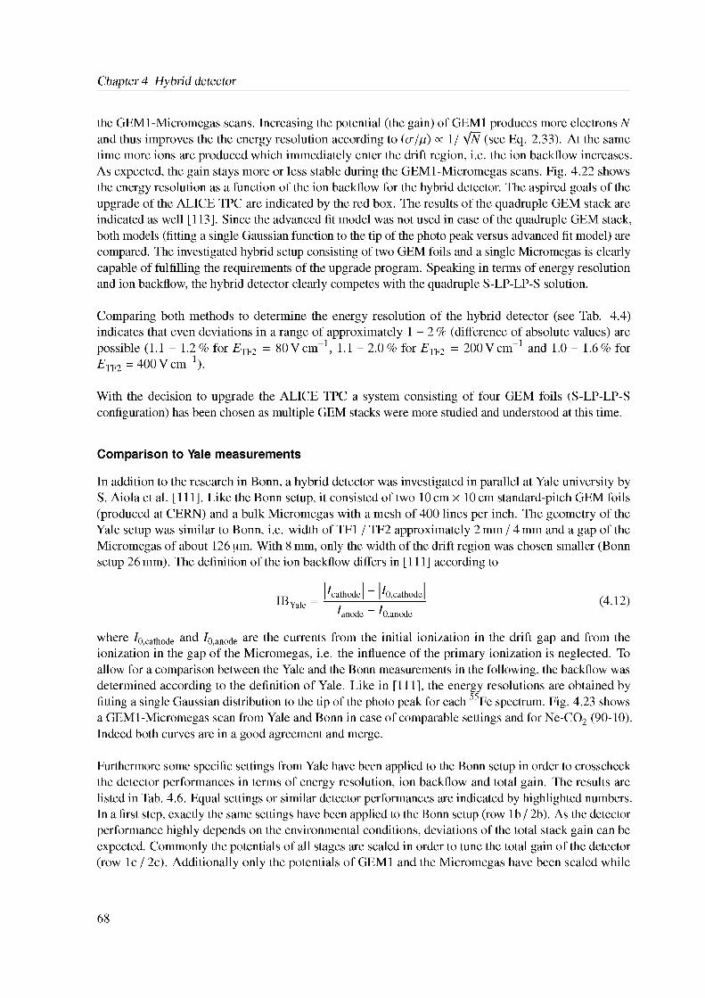
Chapter 4 Hybrid detector
the GEMl-Micromegas scans. Increasing the potential (the gain) of GEM1 produces more electrons N and thus improves the the energy resolution according to (a/p) / 1/VN (see Eq. 2.33). At the same time more ions are produced which immediately enter the drift region, i.e. the ion backflow increases. As expected, the gain stays more or less stable during the GEM1-Micromegas scans. Fig. 4.22 shows the energy resolution as a function of the ion backflow for the hybrid detector. The aspired goals of the upgrade of the ALICE TPC are indicated by the red box. The results of the quadruple GEM stack are indicated as well [113]. Since the advanced fit model was not used in case of the quadruple GEM stack, both models (fitting a single Gaussian function to the tip of the photo peak versus advanced fit model) are compared. The investigated hybrid setup consisting of two GEM foils and a single Micromegas is clearly capable of fulfilling the requirements of the upgrade program. Speaking in terms of energy resolution and ion backflow, the hybrid detector clearly competes with the quadruple S-LP-LP-S solution.
Comparing both methods to determine the energy resolution of the hybrid detector (see Tab. 4.4) indicates that even deviations in a range of approximately 1 - 2 % (difference of absolute values) are possible (1.1 - 1.2% for ETF2 = 80Vcm-1, 1.1 - 2.0% for ETF2 = 200Vcm-1 and 1.0 - 1.6% for ETF2 = 400 V cm"1).
With the decision to upgrade the ALICE TPC a system consisting of four GEM foils (S-LP-LP-S configuration) has been chosen as multiple GEM stacks were more studied and understood at this time.
Comparison to Yale measurements
In addition to the research in Bonn, a hybrid detector was investigated in parallel at Yale university byS. Aiolaetal. [111]. Like the Bonn setup, it consisted of two 10cm x 10 cm standard-pitch GEM foils (produced at CERN) and a bulk Micromegas with a mesh of 400 lines per inch. The geometry of the Yale setup was similar to Bonn, i.e. width of TF1 / TF2 approximately 2 mm / 4 mm and a gap of the Micromegas of about 126 pm. With 8 mm, only the width of the drift region was chosen smaller (Bonn setup 26 mm). The definition of the ion backflow differs in [111] according to
_ | ^cathode | |^0,cathode |Yale = lanode - ^0,anode (4.12)
where /0,cathode and /0,anode are the currents from the initial ionization in the drift gap and from the ionization in the gap of the Micromegas, i.e. the influence of the primary ionization is neglected. To allow for a comparison between the Yale and the Bonn measurements in the following, the backflow was determined according to the definition of Yale. Like in [111], the energy resolutions are obtained by fitting a single Gaussian distribution to the tip of the photo peak for each 55Fe spectrum. Fig. 4.23 shows a GEM1-Micromegas scan from Yale and Bonn in case of comparable settings and for Ne-CO2 (90-10). Indeed both curves are in a good agreement and merge.
Furthermore some specific settings from Yale have been applied to the Bonn setup in order to crosscheck the detector performances in terms of energy resolution, ion backflow and total gain. The results are listed in Tab. 4.6. Equal settings or similar detector performances are indicated by highlighted numbers. In a first step, exactly the same settings have been applied to the Bonn setup (row 1b / 2b). As the detector performance highly depends on the environmental conditions, deviations of the total stack gain can be expected. Commonly the potentials of all stages are scaled in order to tune the total gain of the detector (row 1c / 2c). Additionally only the potentials of GEM1 and the Micromegas have been scaled while
68
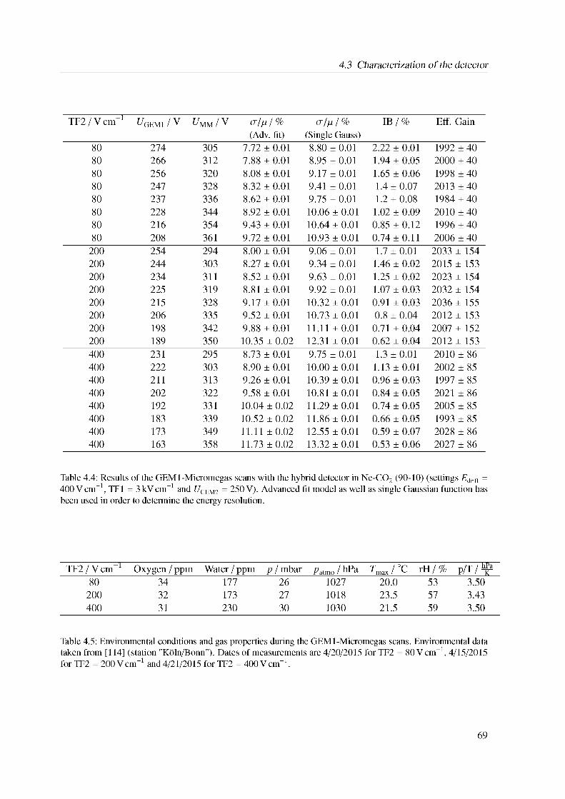
4.3 Characterization of the detector
Table 4.4: Results of the GEMl-Micromegas scans with the hybrid detector in Ne-CO2 (90-10) (settings Edrift = 400 V cm-1, TF1 = 3 kV cm-1 and 17GEM2 = 250 V). Advanced fit model as well as single Gaussian function has been used in order to determine the energy resolution.
TF2 / Vcm-1 ^GEM1 / V ^MM / V alp / % (Adv. fit)
ala / % (Single Gauss)
IB / % Eff. Gain
80 274 305 7.72 ± 0.01 8.80 ± 0.01 2.22 ± 0.01 1992 ± 4080 266 312 7.88 ± 0.01 8.95 ± 0.01 1.94 ± 0.05 2000 ± 4080 256 320 8.08 ± 0.01 9.17 ± 0.01 1.65 ± 0.06 1998 ± 4080 247 328 8.32 ± 0.01 9.41 ± 0.01 1.4 ± 0.07 2013 ± 4080 237 336 8.62 ± 0.01 9.75 ± 0.01 1.2 ± 0.08 1984 ± 4080 228 344 8.92 ± 0.01 10.06 ± 0.01 1.02 ± 0.09 2010 ± 4080 216 354 9.43 ± 0.01 10.64 ± 0.01 0.85 ± 0.12 1996 ± 4080 208 361 9.72 ± 0.01 10.93 ± 0.01 0.74 ± 0.11 2006 ± 40
200 254 294 8.00 ± 0.01 9.06 ± 0.01 1.7 ± 0.01 2033 ± 154200 244 303 8.27 ± 0.01 9.34 ± 0.01 1.46 ± 0.02 2015 ± 153200 234 311 8.52 ± 0.01 9.63 ± 0.01 1.25 ± 0.02 2023 ± 154200 225 319 8.81 ± 0.01 9.92 ± 0.01 1.07 ± 0.03 2032 ± 154200 215 328 9.17 ± 0.01 10.32 ± 0.01 0.91 ± 0.03 2036 ± 155200 206 335 9.52 ± 0.01 10.73 ± 0.01 0.8 ± 0.04 2012 ± 153200 198 342 9.88 ± 0.01 11.11 ± 0.01 0.71 ± 0.04 2007 ± 152200 189 350 10.35 ± 0.02 12.31 ± 0.01 0.62 ± 0.04 2012 ± 153400 231 295 8.73 ± 0.01 9.75 ± 0.01 1.3 ± 0.01 2010 ± 86400 222 303 8.90 ± 0.01 10.00 ± 0.01 1.13 ± 0.01 2002 ± 85400 211 313 9.26 ± 0.01 10.39 ± 0.01 0.96 ± 0.03 1997 ± 85400 202 322 9.58 ± 0.01 10.81 ± 0.01 0.84 ± 0.05 2021 ± 86400 192 331 10.04 ± 0.02 11.29 ± 0.01 0.74 ± 0.05 2005 ± 85400 183 339 10.52 ± 0.02 11.86 ± 0.01 0.66 ± 0.05 1993 ± 85400 173 349 11.11 ± 0.02 12.55 ± 0.01 0.59 ± 0.07 2028 ± 86400 163 358 11.73 ± 0.02 13.32 ± 0.01 0.53 ± 0.06 2027 ± 86
Table 4.5: Environmental conditions and gas properties during the GEM1-Micromegas scans. Environmental data taken from [114] (station "Koln/Bonn"). Dates of measurements are 4/20/2015 for TF2 = 80 Vcm"1, 4/15/2015 for TF2 = 200 V cm-1 and 4/21/2015 for TF2 = 400 V cm-1.
TF2 / Vcm-1 Oxygen / ppm Water / ppm p / mbar Patmo / hPa Tmax / °C rH / % p/T / hKa
80 34 177 26 1027 20.0 53 3.50200 32 173 27 1018 23.5 57 3.43400 31 230 30 1030 21.5 59 3.50
69
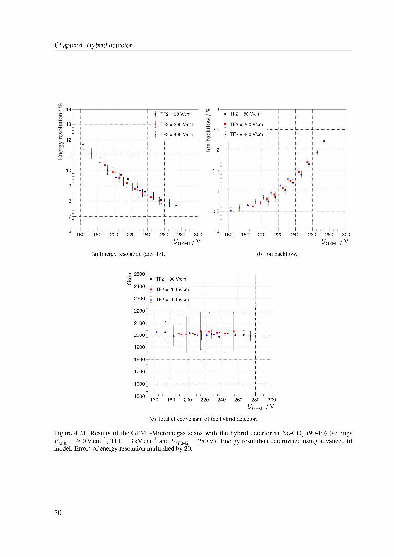
Chapter 4 Hybrid detector
3J TF2 = 80 V/cm
■ TF2 = 200 V/cm
* TF2 = 400 V/cm
14
13
12
11
10
9
8
7
6160 180 200 220 240 260 280 300
^GEM1 I V
2.5
J TF2 = 80 V/cm
■ TF2 = 200 V/cm
* TF2 = 400 V/cm
2 -~4
1 --4
0.5 - -4
0r ill ' ill ' ill ' ill ' 'll ' '[
160 180 200 220 240 260 280 300
^GEM1 I V
1.5 - :
* t
1
(a) Energy resolution (adv. Fit). (b) Ion backflow.
J TF2 = 80 V/cm
■ TF2 = 200 V/cm
* TF2 = 400 V/cm
C 2500
o2400
2300
2200
2100
2000
1900
1800
1700
1600
1500160 180 200 220 240 260 280 300
^GEM11V
(c) Total effective gain of the hybrid detector.
Figure 4.21: Results of the GEM1-Micromegas scans with the hybrid detector in Ne-CO2 (90-10) (settings Edrift = 400 Vcm"1, TF1 = 3kV cm-1 and (7GEM2 = 250 V). Energy resolution determined using advanced fit model. Errors of energy resolution multiplied by 20.
70
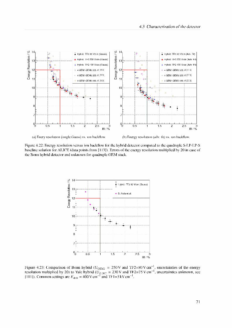
4.3 Characterization of the detector
(a) Enery resolution (single Gauss) vs. ion backflow.
Figure 4.22: Energy resolution versus ion backflow for the hybrid detector compared to the quadruple S-LP-LP-S baseline solution for ALICE (data points from [113]). Errors of the energy resolution multiplied by 20 in case of the Bonn hybrid detector and unknown for quadruple GEM stack.
(b) Energy resolution (adv. fit) vs. ion backflow.
Figure 4.23: Comparison of Bonn hybrid (UGEM2 = 250V and TF2=80Vcm-1, uncertainties of the energy resolution multiplied by 20) to Yale hybrid (UGEM2 = 230 V and TF2=75 Vcm-1, uncertainties unknown, see [111]). Common settings are Edrift = 400Vcm-1 andTF1=3kVcm-1.
71
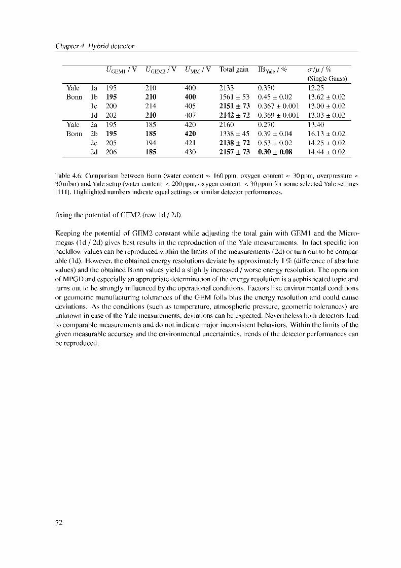
Chapter 4 Hybrid detector
Table 4.6: Comparison between Bonn (water content ~ 160 ppm, oxygen content ~ 30 ppm, overpressure ~ 30mbar) and Yale setup (water content < 200 ppm, oxygen content < 30 ppm) for some selected Yale settings [111]. Highlighted numbers indicate equal settings or similar detector performances.
^GEM1 / V ^GEM2 / V ^MM / V Total gain IBYale / % a/p / % (Single Gauss)
Yale 1a 195 210 400 2133 0.350 12.25Bonn 1b 195 210 400 1561±53 0.45 ± 0.02 13.62 ± 0.02
1c 200 214 405 2151 ± 73 0.367 ± 0.001 13.00 ± 0.021d 202 210 407 2142 ± 72 0.369 ± 0.001 13.03 ± 0.02
Yale 2a 195 185 420 2160 0.270 13.40Bonn 2b 195 185 420 1338 ± 45 0.39 ± 0.04 16.13 ± 0.02
2c 205 194 421 2138 ± 72 0.53 ± 0.02 14.25 ± 0.022d 206 185 430 2157 ± 73 0.30 ± 0.08 14.44 ± 0.02
fixing the potential of GEM2 (row 1d / 2d).
Keeping the potential of GEM2 constant while adjusting the total gain with GEM1 and the Micromegas (1d / 2d) gives best results in the reproduction of the Yale measurements. In fact specific ion backflow values can be reproduced within the limits of the measurements (2d) or turn out to be comparable (1d). However, the obtained energy resolutions deviate by approximately 1 % (difference of absolute values) and the obtained Bonn values yield a slightly increased / worse energy resolution. The operation of MPGD and especially an appropriate determination of the energy resolution is a sophisticated topic and turns out to be strongly influenced by the operational conditions. Factors like environmental conditions or geometric manufacturing tolerances of the GEM foils bias the energy resolution and could cause deviations. As the conditions (such as temperature, atmospheric pressure, geometric tolerances) are unknown in case of the Yale measurements, deviations can be expected. Nevertheless both detectors lead to comparable measurements and do not indicate major inconsistent behaviors. Within the limits of the given measurable accuracy and the environmental uncertainties, trends of the detector performances can be reproduced.
72
CHAPTER 5
A model for charge transfer in GEM foils
5.1 Charge transfer in GEM foils
The ion backflow, the energy resolution as well as the gain of GEM stacks highly depend on the charge transfer processes between the different GEM stages. Thus a good understanding of the transfer processes is mandatory. Commonly these processes can be described using the collection and extraction efficiency for the charge carriers of a GEM. The charge transfer processes can be characterized as follows:
• The electron collection efficiency (e~oll) is defined as the ratio between the number of electrons entering the holes (i.e. number NColl of electrons which are not blocked by the top electrode of the GEM) and the number of electrons approaching the GEM foil (N0).
- _ Ncoll'c"" No (5.1)
• The electron extraction efficiency (qTxtr) is defined as the ratio between the number of electrons extracted from the holes (i.e. number Ne"xtr of electrons reaching the next amplification stage / readout plane) and the total number of electrons available in the holes after the multiplication (N^).
eextrNextr
N~ J’in(5.2)
Generally the average (macroscopic) movement of the charge carriers is defined by the electric and the magnetic field according to the Langevin equation (Eq. 2.20). In this approach no magnetic field has been taken into account and the efficiencies will be modeled by calculating the electric field inside a GEM hole. Fig. 5.1 shows the electric field lines inside a GEM hole for a standard-pitch GEM based on the calculations of the electric fields which will part in the following chapter. The field lines have been calculated for different ratios of the electric fields above / below the GEM (Eabove and Ebelow) and inside the GEM hole Egem1. Field lines with common origin and ending positions are indicated by the same color. Fig. 5.1(a) shows field lines originating from the cathode for a high field above the GEM, i.e. some field lines end on the top side of the GEM (magenta). The remaining field lines (yellow) enter and leave the hole at the bottom side of the GEM. For a low field above the GEM, no field lines from the cathode end on the top side of the GEM (Fig. 5.1(b)). In this case only field lines originate from
1 A detailed discussion about the ratios and the calculations "f the electric fields will be part "f Sec. 5.2.3.
73
Chapter 5 A model for charge transfer in GEM foils
the top side of the GEM (Fig. 5.1(c)). While some of the field lines manage to reach the anode (green), some of them may end at the bottom side of the GEM (orange). If the field below the GEM is sufficiently high (Fig. 5.1(d)), field lines will additionally start at the bottom side and end at the anode (blue).
All these common field lines can be combined to several electric fluxes within a GEM hole. Generally the electric flux p through a certain region (or surface A with orthogonal normal vector ft) is defined as the surface integral of the electric field f according to
p = I'/' dA (5.3)Ja
where dA = ft dA. The collection as well as the extraction efficiency that have been defined above in terms of number of electrons can alternatively be defined as a function of the electric fluxes inside a GEM. This has been studied by Killenberg et al. [115]. A schematic view of all common field lines from Fig.5.1 is shown in Fig. 5.2 as electric fluxes. The electron collection efficiency can be defined as the part D of the total flux pcath which enters the GEM hole. The extraction efficiency of a GEM is defined as the ratio of the flux through the hole which reaches the anode (given by the sum of flux D and the ring-shaped flux R, i.e. D + R) compared to the total flux phole through the hole. In [115] Killenberg gets the electric flux by performing a numerical simulation using the the finite element program Maxwell 3D. It allows to solve Maxwell’s equations for a three-dimensional problem. The obtained results are thereupon parameterized in order to describe the collection and extraction efficiency. The parametrization is later used to predict the transfer properties of a GEM. An approach that is based on the same methodology can be found by Bencivenni et al. in [116]. Also here a parametrization of the efficiencies has been used to predict measurements of the transfer processes. However, both parameterizations do not fully explain the behavior of three different regions that can be clearly seen in the data. In addition measurements and simulations reveal that the extraction efficiency for electrons has an offset that is not included in the parametrization.
Based on the following electric flux calculations, analytic expressions can be found for the collection and extraction efficiency by modeling a GEM as a two-dimensional charge density distribution. Effects like diffusion and charge carrier losses caused by attachment are not taken into account. The obtained results inherently include an offset for the extraction efficiency and predict the appropriate limits for a GEM.
5.2 Efficiency calculations based on an analytic two-dimensional model
5.2.1 Charge-density model
The electric fluxes and thus the efficiencies are calculated analytically based on a simplified twodimensional cut through the hexagonal GEM structure. The top and the bottom side of the GEM are modeled by metal electrodes carrying constant electric line charges. A central assumption in this work are the constant charge density distributions which cause nonconstant potentials on the electrodes. The dielectric polyimide layer between the top and the bottom side is ignored, i.e. a differentiation between an inner and an outer hole diameter is not considered. Based on the charge density p for this configuration the electric potential can be obtained by solving Poisson’s equation AV = -ple0. The electric field is thereupon given by E = -VV. The electric fluxes can then be calculated according to Eq. 5.3 which
74
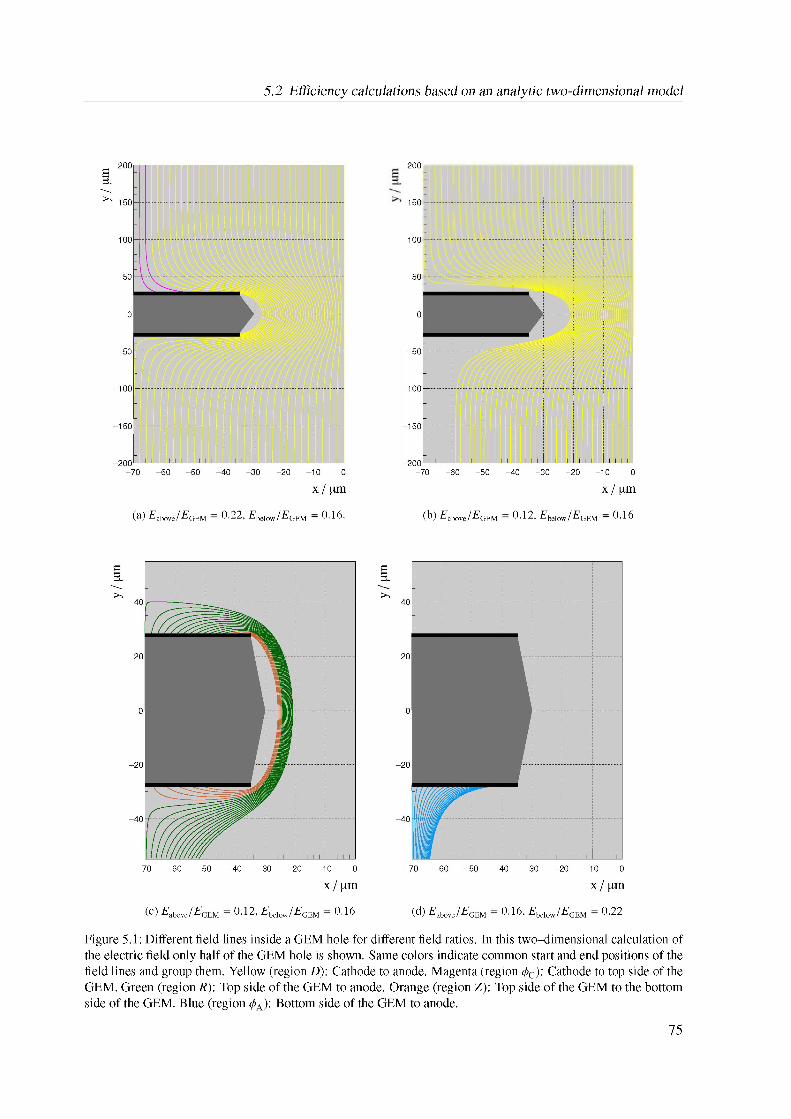
5.2 Efficiency calculations based on an analytic two-dimensional model
(a) Eabove/EGEM 0.22, Ebelow/EGEM = 0.16-
200
150
100
50
-70 -60 -50 -40 -30 -20 -10 0
x / [im
(b) Eabove/EGEM 0.12, Ebelow/EGEM = 0.16
-70 -60 -50 -40 -30 -20 -10 0
x / |im
(d) Eabove/EGEM = 0d6, Ebelow/EGEM = 0.22Figure 5.1: Different field lines inside a GEM hole for different field ratios. In this two-dimensional calculation of the electric field only half of the GEM hole is shown. Same colors indicate common start and end positions of the field lines and group them. Yellow (region D): Cathode to anode. Magenta (region 0C): Cathode to top side of the GEM. Green (region R): Top side of the GEM to anode. Orange (region Z): Top side of the GEM to the bottom side of the GEM. Blue (region 0A): Bottom side of the GEM to anode.
(c) Eabove/EGEM = 0.12, Ebelow/EGEM = 0.16
75
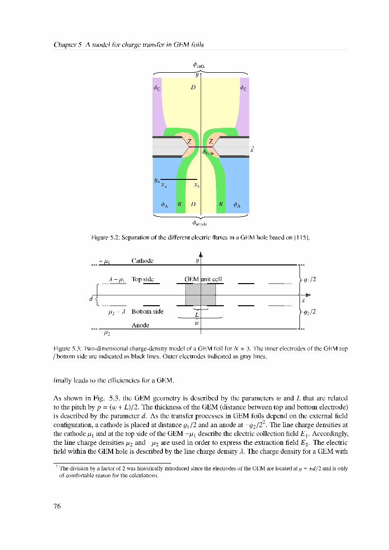
Chapter 5 A model for charge transfer in GEM foils
Figure 5.2: Separation of the different electric fluxes in a GEM hole based on [115].
+ p Cathode y
A - p Top side GEM unit cell ►g1/2
d -
p2 - A Bottom side L-■--- i--- --------
X
>92/
Anode w- P2
Figure 5.3: Two-dimensional charge-density model of a GEM foil for N = 3. The inner electrodes of the GEM top / bottom side are indicated as black lines. Outer electrodes indicated as gray lines.
finally leads to the efficiencies for a GEM.
As shown in Fig. 5.3, the GEM geometry is described by the parameters w and L that are related to the pitch by p = (w + L)/2. The thickness of the GEM (distance between top and bottom electrode) is described by the parameter d. As the transfer processes in GEM foils depend on the external field configuration, a cathode is placed at distance g1 /2 and an anode at -g2/22. The line charge densities at the cathode p1 and at the top side of the GEM -p1 describe the electric collection field E1. Accordingly, the line charge densities p2 and -p2 are used in order to express the extraction field E2. The electric field within the GEM hole is described by the line charge density A. The charge density for a GEM with
2 The division by a factor of 2 was historically introduced since the electrodes of the GEM are located at y = +d/2 and is only of comfortable reason for the calculations.
76
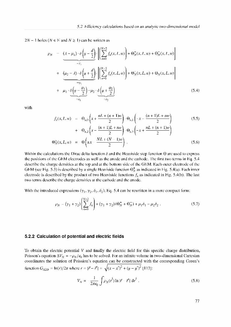
5.2 Efficiency calculations based on an analytic two-dimensional model
2N - 1 holes (N e N and N > 1) can be written as
Pn (2 - pO • s| {Z
0N-2 1
fn(x; L; w)\n=0 /
+ ©N(x, L, w) + ©N(x, L, w)
=71
(P2 - 2 • S
| {Z
0N-2 1W 1 / 1 fn(x; L; w)
\n=0 /+ ©N(x, L, w) + ©N(x, L, w)
=72
J d1\Pi • s\y - 21 -^2 •
' =S1 ^
(5.4)
with
fn(x, L,w) ©n,0 x + nL + (n + 1)w 2
(n + 1)L + nw2
(n + 1)L + nw2 (5.5)
©N(x, L, w)NL + (N - 1)w
2
/ nL + (n + 1)w ©n,3 ~x + -------5---------
(5.6)
Within the calculations the Dirac delta function S and the Heaviside step function © are used to express the positions of the GEM electrodes as well as the anode and the cathode. The first two terms in Eq. 5.4 describe the charge densities at the top and at the bottom side of the GEM: Each outer electrode of the GEM (see Fig. 5.3) is described by a single Heaviside function ©N as indicated in Fig. 5.4(a). Each inner electrode is described by the product of two Heaviside functions fn as indicated in Fig. 5.4(b). The last two terms describe the charge densities at the cathode and the anode.
With the introduced expressions (y1, 72, S1, S2), Eq. 5.4 can be rewritten in a more compact form:
0N-2 1
Pn = (71 + 72) V fn + (71 + 72) (©N + ©N) + P1S1 - P2S2 • (5.7)n=0
5.2.2 Calculation of potential and electric fields
To obtain the electric potential V and finally the electric field for this specific charge distribution, Poisson’s equation AVN = -pN/e0 has to be solved. For an infinite volume in two-dimensional Cartesian coordinates the solution of Poission’s equation can be constructed with the corresponding Green’s function GA2D = ln(r)/2^ where r = ~- f\ = J(x - x')2 + (y - y0)2 [117]:
Vn = -7^ fpN(r')ln\r-/| dr' • 2^0 J
(5.8)
77
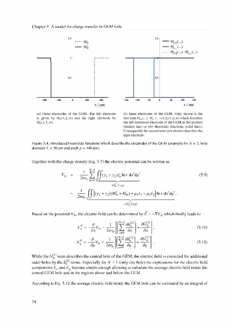
Chapter 5 A model for charge transfer in GEM foils
(a) Outer electrodes of the GEM. The left electrode is given by ®N (x, L,w) and the right electrode by ®N(x, L, w).
(b) Inner electrodes of the GEM. Only shown is the first term ®„,0(...)' ®n,1(---) of f0(x, L, w) which describes the left innermost electrode of the GEM as the product (dashed line) of two Heaviside functions (solid lines). Consequently the second term (not shown) describes the right electrode.
Figure 5.4: Introduced Heaviside functions which describe the electrodes of the GEM (example for N = 3, hole diameter L = 50 pm and pitch p = 140 pm).
Together with the charge density (Eq. 5.7) the electric potential can be written as
1 X 2VN = - 2^7 JJ (j1 + 72)fn ln r dX dyf
n 0 | {Z }=^ni)(x,y)
- 2~rff [(71 + 72) (®N + ®N) + M1 - ^2] ln r dxdy' .
| {Z }=oN)(x,y)
(5.9)
Based on the potential VN, the electric field can be determined by E = -WN which finally leads to
eNx@vn =... Ilx '|+
L\n=0
EnEy
@ V = 1 By2@h«}CC + @GN
@y N 2..0 B £0 @y C @y
(5.10)
(5.11)
While the G'N! term describes the central hole of the GEM, the electric field is corrected for additional outer holes by the h(1 terms. Especially for N = 1 (only one hole) the expressions for the electric field components Ex and Ey become simple enough allowing to calculate the average electric field inside the central GEM hole and in the regions above and below the GEM.
According to Eq. 5.12 the average electric field inside the GEM hole can be estimated by an integral of
78
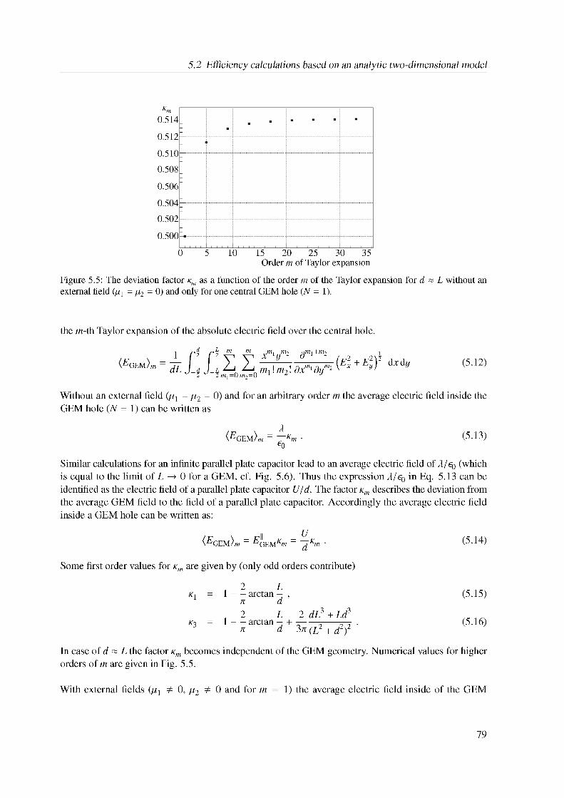
5.2 Efficiency calculations based on an analytic two-dimensional model
m0.514
0.512
0.510
0.508
0.506
0.504
0.502
0.500
0 5 10 15 20 25 30 35Order m of Taylor expansion
Figure 5.5: The deviation factor Km as a function of the order m of the Taylor expansion for d ~ L without an external field (ji1 = p2 = 0) and only for one central GEM hole (N = 1).
the m-th Taylor expansion of the absolute electric field over the central hole.
+'•2d L
(EGEm) mXm1 ym2 @m1+m2
m1! m2! dxm1 dyimdx dy (5.12)E
Without an external field (/^ = p2 = 0) and for an arbitrary order m the average electric field inside the GEM hole (N = 1) can be written as
(EGEm)m = ~Km . e0
(5.13)
Similar calculations for an infinite parallel plate capacitor lead to an average electric field of T/e0 (which is equal to the limit of L ! 0 for a GEM, cf. Fig. 5.6). Thus the expression T/e0 in Eq. 5.13 can be identified as the electric field of a parallel plate capacitor U/d. The factor Km describes the deviation from the average GEM field to the field of a parallel plate capacitor. Accordingly the average electric field inside a GEM hole can be written as:
(EGEM}m = EGEMKm = ~dd Km ' (5.14)
Some first order values for Km are given by (only odd orders contribute)
Ki = 1 - - arctan ,- d
(5.15)
2 L 2 dL3 + Ld3‘ = 1 - - - + 3^ (l3 + d2?. (5.16)
In case of d « L the factor Km becomes independent of the GEM geometry. Numerical values for higher orders of m are given in Fig. 5.5.
With external fields (^1 , 0, p2 , 0 and for m = 1) the average electric field inside of the GEM
79
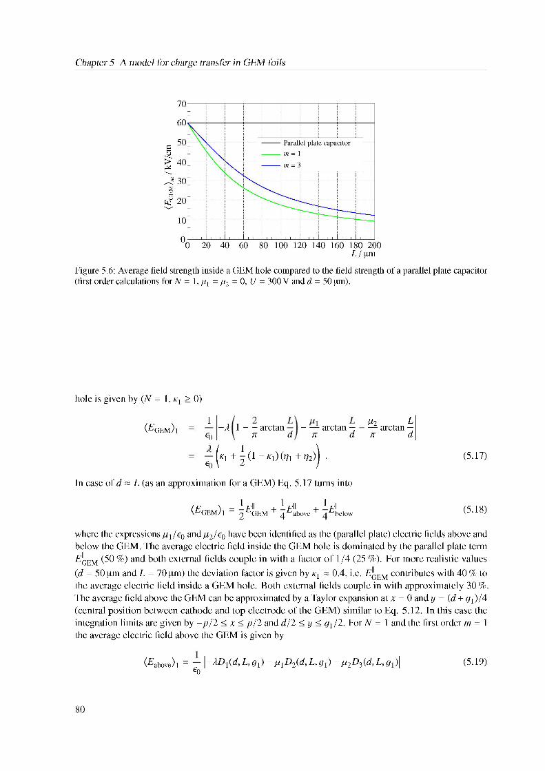
Chapter 5 A model for charge transfer in GEM foils
Figure 5.6: Average field strength inside a GEM hole compared to the field strength of a parallel plate capacitor (first order calculations for N = 1, p1 = p.2 = 0, U = 300 V and d = 50 pm).
hole is given by (N = 1, k1 > 0)
(EGEm)11
e0-A 1 - - arctan - — arctan 3
n d n dh2 , L— arctan — n d
^~^1+211 _ *1)(^1+%)) •
In case of d « L (as an approximation for a GEM) Eq. 5.17 turns into
(Eg ) = 1E1 + 1E11. + 1 Ej .GEM1 2 GEM 4 above 4 below
(5.17)
(5.18)
where the expressions p1 /e0 and p2/e0 have been identified as the (parallel plate) electric fields above and below the GEM. The average electric field inside the GEM hole is dominated by the parallel plate term eGEM (50 %) and both external fields couple in with a factor of 1 /4 (25 %). For more realistic values (d = 50 pm and L = 70 pm) the deviation factor is given by k1 & 0:4, i.e. eGem contributes with 40 % to the average electric field inside a GEM hole. Both external fields couple in with approximately 30 %. The average field above the GEM can be approximated by a Taylor expansion at x = 0 and y = (d + g1)/4 (central position between cathode and top electrode of the GEM) similar to Eq. 5.12. In this case the integration limits are given by -p/2 < x < p/2 and d/2 < y < g1 /2. For N = 1 and the first order m = 1 the average electric field above the GEM is given by
(Eaboveh = — \-AD1(d, L,Q1) - P1 D2(.d, L,Q1) - P2D3(d, L,Q1)\ (5.19)e0
80
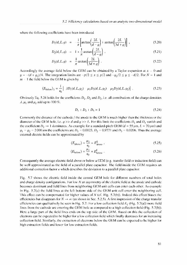
5.2 Efficiency calculations based on an analytic two-dimensional model
where the following coefficients have been introduced
1n
D1(d, L,g)
D2(d, L, g)
D3(d, L,g)
arctan
- arctan [ n \d - g
1- arctan n
(5.20)
(5.21)
(5.22)
1 +
Accordingly the average field below the GEM can be obtained by a Taylor expansion at x = 0 and y = -(d + g2)/4. The integration limits are -p/2 < x < p/2 and -g2/2 < y < -d/2. For N = 1 and m = 1 the field below the GEM is given by
(Ebelow)1 = |-dD1(d, L,g2) _ P1 D3(d, L,g2) _ P2D2(d, L, g2)| ■e0
(5.23)
Obviously Eq. 5.24 holds for the coefficients D1, D2 and D3, i.e. all contributions of the charge densities A, p1 and p2 add up to 100 %.
D1 + D2 + D3 = 1 (5.24)
Commonly the distance of the cathode / the anode to the GEM is much higher than the thickness or the diameter of the GEM hole, i.e. g >> d and g >> L. For this limit the coefficients D1 and D3 vanish and the coefficient D2 ! 1 dominates. As example for a standard-pitch GEM (d = 55 pm, L = 70 pm) and g1 = g2 = 2000 pm the coefficients are D1 = 0:0023, D2 = 0:9771 and D3 = 0:0206. Thus the average external electric fields can be approximated by
E a » ( = Bjbove . (5.25)e0
V »= E., ■ (5-26)e0
Consequently the average electric field above or below a GEM (e.g. transfer field or induction field) can be well approximated as the field of a parallel plate capacitor. The field inside the GEM requires an additional correction factor k which describes the deviation to a parallel plate capacitor.
Fig. 5.7 shows the electric field inside the central GEM hole for different numbers of total holes and charge density configurations. For low N an asymmetry of the electric field at the anode and cathode becomes dominant and field lines from neighboring GEM unit cells can enter each other. As example in Fig. 5.7(c) the field lines at the left bottom side of the GEM unit cell enter the neighboring cell. This effect can be compensated for higher values of N (cf. Fig. 5.7(b)). Indeed this effect biases the efficiencies but disappears for N ! 1 (as shown in Sec. 5.2.5). A first impression of the charge transfer efficiencies can qualitatively be seen in Fig. 5.7: For a low collection field E1 (Fig. 5.7(a)) more field lines from the cathode are entering the GEM hole as compared to a high collection field (Fig. 5.7(b)). Here a large part of the field lines ends on the top side of the GEM. Based on this the collection of electrons can be expected to be higher for a low collection field which finally decreases for an increasing collection field. Similarly, the extraction of electrons below the GEM can be expected to be higher for high extraction fields and lower for low extraction fields.
81
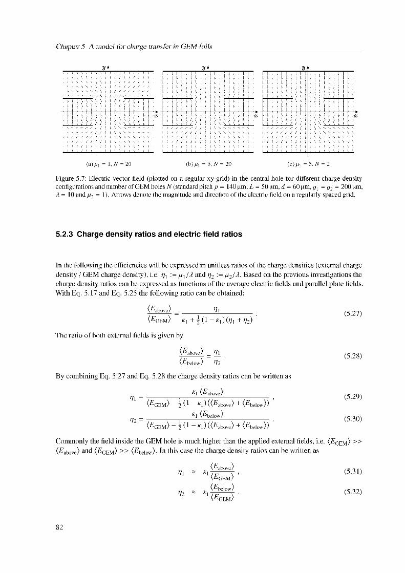
Chapter 5 A model for charge transfer in GEM foils
Figure 5.7: Electric vector field (plotted on a regular xy-grid) in the central hole for different charge density configurations and number of GEM holes N (standard pitch p = 140 pm, L = 50 pm, d = 60 pm, g1 = g2 = 200 pm, A = 10 and p2 = 1). Arrows denote the magnitude and direction of the electric field on a regularly spaced grid.
5.2.3 Charge density ratios and electric field ratios
(5.27)
(5.28)
(5.29)
(5.30)
In the following the efficiencies will be expressed in unitless ratios of the charge densities (external charge density / GEM charge density), i.e. p1 := p11A and 72 := p2/A. Based on the previous investigations the charge density ratios can be expressed as functions of the average electric fields and parallel plate fields. With Eq. 5.17 and Eq. 5.25 the following ratio can be obtained:
(Eabove7 = 71
(EGEm) *1 + 2 (1 - K1) (P1 + ^2)
The ratio of both external fields is given by
(Eabove) = 71
(Ebelow) 7 2
By combining Eq. 5.27 and Eq. 5.28 the charge density ratios can be written as
*1 (Eabove)71 = 1;
(EGEm) “ 2 C1 “ *1) ((EabovJ + (Ebelow))
*1 (Ebelow)72 = 777^77 •(EGEm) 2 1 *1) ((Eabove) + (Ebelow))
Commonly the field inside the GEM hole is much higher than the applied external fields, i.e. (Egem) >> (Eabove) and (Egem) >> (Ebelow). In this case the charge density ratios can be written as
71
72
(Eabove)1 (EGEM 7
(Ebelow71 (egem7
(5.31)
(5.32)
82
5.2 Efficiency calculations based on an analytic two-dimensional model
By using Eq. 5.17, 5.25 and 5.26 the charge density ratios (Eq. 5.29 and 5.30) can be expressed as functions of the parallel external fields
E11 above* = I.
GEM
Eb elow % = j
GEM
(5.33)
(5.34)
5.2.4 Flux calculations and efficiencies
As shown in Fig. 5.2, the field inside a GEM can be separated into several fluxes [115]. The collection efficiency (Eq. 5.35) can be expressed as the part D of the total cathode flux 0cath which enters the GEM hole. For common GEM settings all field lines originating from the cathode point to the GEM foil. Depending on the field configuration, some of them might end on the top electrodes of the GEM (flux 0C). These field lines point downwards (i.e. negative y-component) at the top side of the GEM. The flux 0C is adjoined by the flux R. At the top side of the GEM, the field lines from flux R point upwards (i.e. positive y-component). By finding the point on the top side of the GEM where the electric field in y-direction E^ changes the sign gives access to calculate <pC and finally the collection efficiency. The flux $C can be calculated as it corresponds to all field lines which end on the top side of the GEM (point downwards, i.e. negative y-component) and which is adjoined by the flux R which field lines originate from the GEM (point upwards, i.e. positive y-component).
ecoll
Gxtr
D _ ^cath 2^C
^cath ^cath
D + 2R _ ^anode ~ ''''•' A
0hole 0hole
(5.35)
(5.36)
The extraction efficiency (Eq. 5.36) of a GEM is defined as the flux D + 2R through the hole 0hole which manages to reach the anode. The flux D + 2R can be expressed by the flux <pA which again can be found by a flip of the electric field in y-direction at the bottom side of the GEM.
In general the electric flux <p through an arbitrary two-dimensional surface which is parallel to the GEM (starting from xa to xb at ya) can be calculated according to Eq. 5.37. For the following calculations the direction of the limit is of importance which is notated by y± (+ limit from top side, - limit from bottom side).
1<p _ f E dA _ — lim
J a 2^e0 y!y„
0N-2X P ffill dxC + f
n_00Jxa dy A\n_0
dx (5.37)x @gN)
a dy
Collection efficiency
In order to calculate the collection efficiency the fluxes 0cath and 0C need to be known. The flux at the cathode 0cath can be calculated according to Eq. 5.37 with xa _ -(w + L)/4, xb _ (w + L)/4 and y ! (g1 /2)~. The calculation of the flux 0C turns out to be more complicated since three different cases need to be considered for xb .
1. Plateau region (Fig. : For low collection field ratios ^1 all field lines on the top side of the 5.9(a))
83
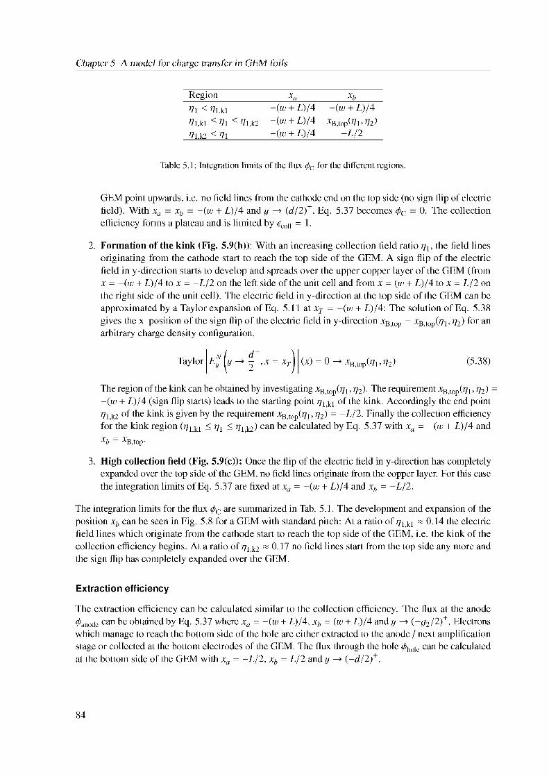
Chapter 5 A model for charge transfer in GEM foils
Table 5.1: Integration limits of the flux </>C for the different regions.
Region xa xb
71 < 71,k1 —(w + L)/4 —(w + L)/471, k1 ^ 71 ^ 71, k2 —(w + L)/4 xB,top(71; 72)71,k2 < 71 —(w + L)/4 -L/2
GEM point upwards, i.e. no field lines from the cathode end on the top side (no sign flip of electric field). With xa = xb = -(w + L)/4 and y ! (d/2)+, Eq. 5.37 becomes 0C = 0. The collection efficiency forms a plateau and is limited by ecoll = 1.
2. Formation of the kink (Fig. 5.9(b)): With an increasing collection field ratio 71, the field lines originating from the cathode start to reach the top side of the GEM. A sign flip of the electric field in y-direction starts to develop and spreads over the upper copper layer of the GEM (from x = -(w + L)/4 to x = -L/2 on the left side of the unit cell and from x = (w + L)/4 to x = L/2 on the right side of the unit cell). The electric field in y-direction at the top side of the GEM can be approximated by a Taylor expansion of Eq. 5.11 at xT = -(w + L)/4: The solution of Eq. 5.38 gives the x-position of the sign flip of the electric field in y-direction xB,top = xB,top(71, 72) for an arbitrary charge density configuration.
Taylor EnEy (x) = 0 ! xB,top(71;72) (5.38)
The region of the kink can be obtained by investigating xB,top(71, 72). The requirement xB,top(71,72) = -(w + L)/4 (sign flip starts) leads to the starting point 71,k1 of the kink. Accordingly the end point 71;k2 of the kink is given by the requirement xB,top(71, 72) = -L/2. Finally the collection efficiency for the kink region (71,k1 ^ 71 < ^1,k2) can be calculated by Eq. 5.37 with xa = -(w + L)/4 and xb = xB;top.
3. High collection field (Fig. 5.9(c)): Once the flip of the electric field in y-direction has completely expanded over the top side of the GEM, no field lines originate from the copper layer. For this case the integration limits of Eq. 5.37 are fixed at xa = -(w + L)/4 and xb = -L/2.
The integration limits for the flux <pC are summarized in Tab. 5.1. The development and expansion of the position xb can be seen in Fig. 5.8 for a GEM with standard pitch: At a ratio of 71,k1 ~ 0.14 the electric field lines which originate from the cathode start to reach the top side of the GEM, i.e. the kink of the collection efficiency begins. At a ratio of 71;k2 ~ 0.17 no field lines start from the top side any more and the sign flip has completely expanded over the GEM.
Extraction efficiency
The extraction efficiency can be calculated similar to the collection efficiency. The flux at the anode 0anode can be obtained by Eq. 5.37 where xa = -(w + L)/4, xb = (w + L)/4 and y ! (-g2/2)+. Electrons which manage to reach the bottom side of the hole are either extracted to the anode / next amplification stage or collected at the bottom electrodes of the GEM. The flux through the hole 0hole can be calculated at the bottom side of the GEM with xa = -L/2, xb = L/2 and y ! (-d/2)+.
84
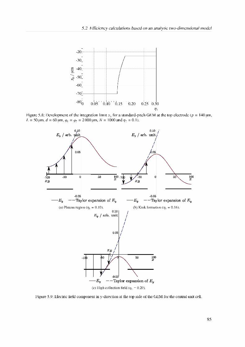
5.2 Efficiency calculations based on an analytic two-dimensional model
Figure 5.8: Development of the integration limit xb for a standard-pitch GEM at the top electrode (p = 140 pm, L = 50 pm, d = 60 pm, g = g2 = 2 000 pm, N = 1000 and ^2 = 0.1).
(c) High collection field (^1 = 0.20).
Figure 5.9: Electric field component in y-direction at the top side of the GEM for the central unit cell.
85
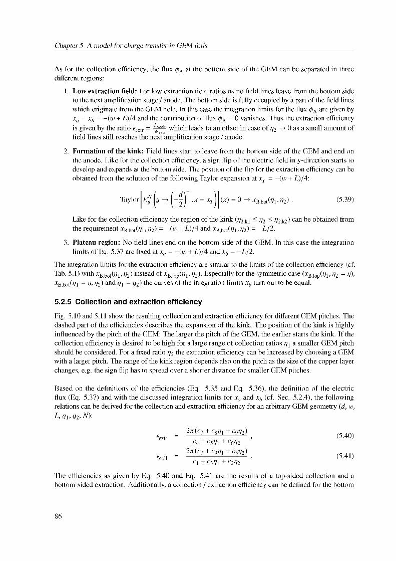
Chapter 5 A model for charge transfer in GEM foils
As for the collection efficiency, the flux 0A at the bottom side of the GEM can be separated in three different regions:
1. Low extraction field: For low extraction field ratios p2 no field lines leave from the bottom side to the next amplification stage / anode. The bottom side is fully occupied by a part of the field lines which originate from the GEM hole. In this case the integration limits for the flux <pA are given by xa = xb = ~(w + L)/4 and the contribution of flux <pA = 0 vanishes. Thus the extraction efficiency is given by the ratio eextr = ^A^- which leads to an offset in case of p2 ! 0 as a small amount of field lines still reaches the next amplification stage / anode.
2. Formation of the kink: Field lines start to leave from the bottom side of the GEM and end on the anode. Like for the collection efficiency, a sign flip of the electric field in y-direction starts to develop and expands at the bottom side. The position of the flip for the extraction efficiency can be obtained from the solution of the following Taylor expansion at xT = -(w + L)/4:
Taylor (X) = 0 ! XB;bot(ffi,%) • (5.39)
Like for the collection efficiency the region of the kink (h2,k1 ^ h2 < h2,k2) can be obtained from the requirement xB,bot(h1, h2) = -(w + L)/4 and xB,bot(h1, h2) = -L/2.
3. Plateau region: No field lines end on the bottom side of the GEM. In this case the integration limits of Eq. are fixed at xa = -(w + L)/4 and xb = -L/2. 5.37
The integration limits for the extraction efficiency are similar to the limits of the collection efficiency (cf. Tab. 5.1) with xB,bot(h1, h2) instead of xB,top(h1, h2). Especially for the symmetric case (xB,top(h1, p2 = h), xB,bot(h1 = h, h2) and g1 = g2) the curves of the integration limits xb turn out to be equal.
5.2.5 Collection and extraction efficiency
Fig. 5.10 and 5.11 show the resulting collection and extraction efficiency for different GEM pitches. The dashed part of the efficiencies describes the expansion of the kink. The position of the kink is highly influenced by the pitch of the GEM: The larger the pitch of the GEM, the earlier starts the kink. If the collection efficiency is desired to be high for a large range of collection ratios h1 a smaller GEM pitch should be considered. For a fixed ratio h2 the extraction efficiency can be increased by choosing a GEM with a larger pitch. The range of the kink region depends also on the pitch as the size of the copper layer changes, e.g. the sign flip has to spread over a shorter distance for smaller GEM pitches.
Based on the definitions of the efficiencies (Eq. 5.35 and Eq. 5.36), the definition of the electric flux (Eq. 5.37) and with the discussed integration limits for xa and xb (cf. Sec. 5.2.4), the following relations can be derived for the collection and extraction efficiency for an arbitrary GEM geometry (d, w, L, 01, 02,N):
^extr
ecoll
2^ (c7 + c8d1 + c9^2) c4 + c501 + c602
2^ (c7 + c9h1 + c8^2)
c1 + c3^1 + c2^2
(5.40)
(5.41)
The efficiencies as given by Eq. 5.40 and Eq. 5.41 are the results of a top-sided collection and a bottom-sided extraction. Additionally, a collection / extraction efficiency can be defined for the bottom
86
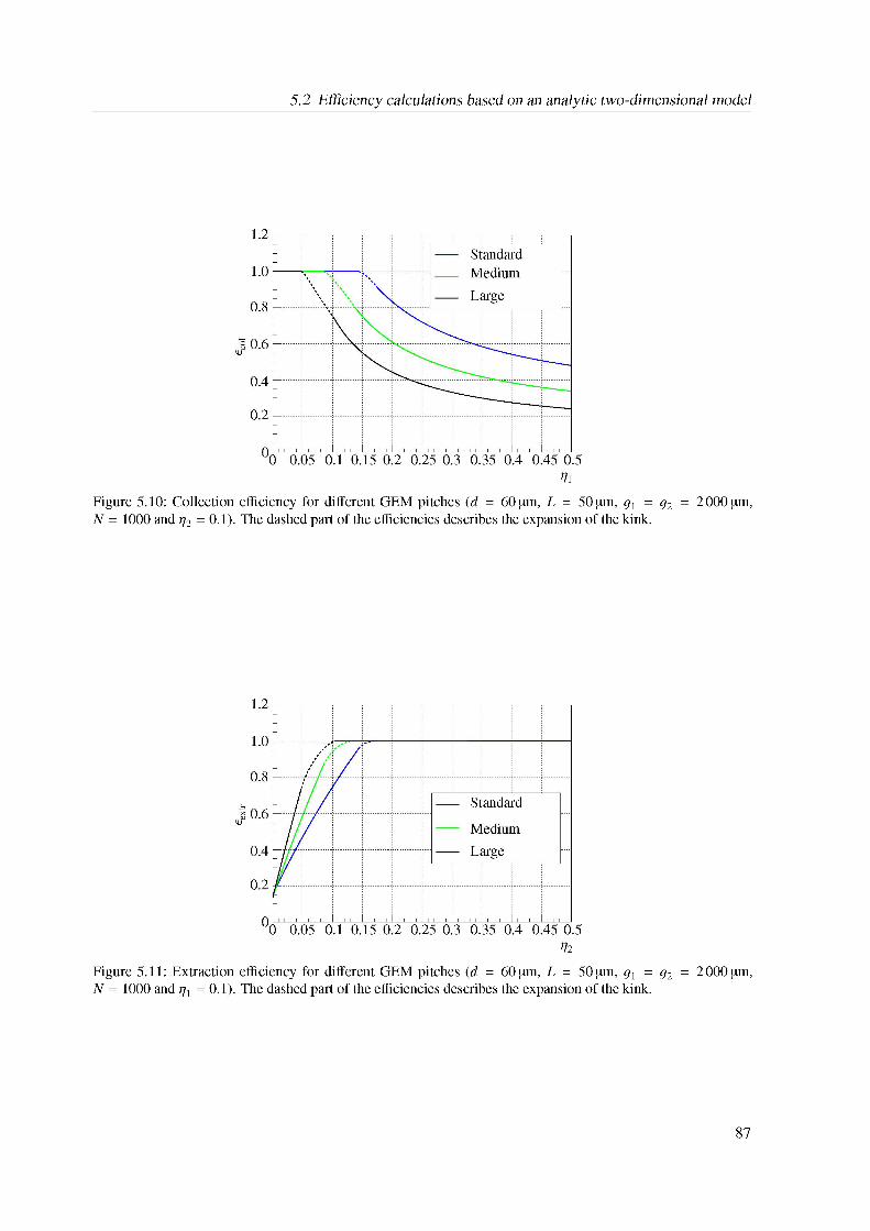
5.2 Efficiency calculations based on an analytic two-dimensional model
Figure 5.10: Collection efficiency for different GEM pitches (d = 60 pm, L = 50 pm, g1 = g2 = 2000 pm, N = 1000 and g2 = 0.1). The dashed part of the efficiencies describes the expansion of the kink.
Figure 5.11: Extraction efficiency for different GEM pitches (d = 60 pm, L = 50 pm, g1 = g2 = 2000 pm, N = 1000 and g1 = 0.1). The dashed part of the efficiencies describes the expansion of the kink.
87
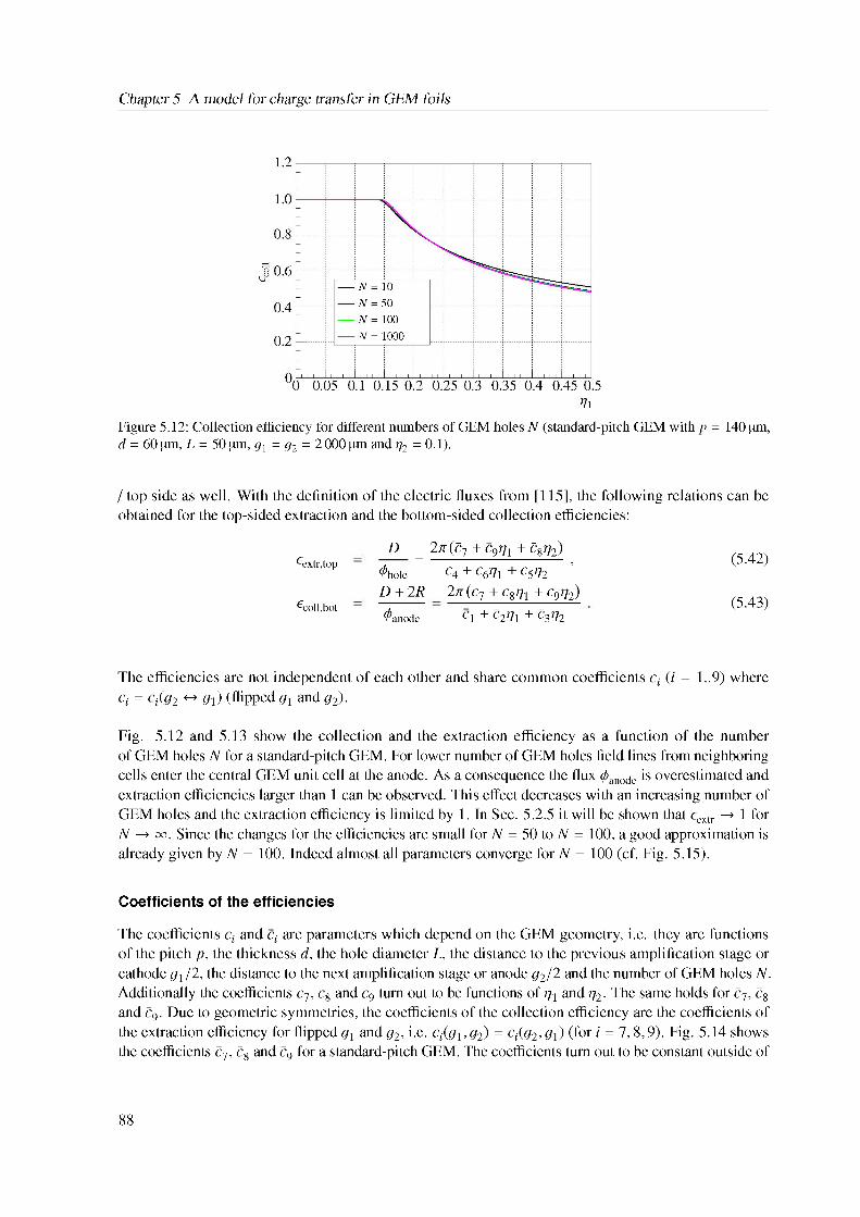
Chapter 5 A model for charge transfer in GEM foils
Figure 5.12: Collection efficiency for different numbers of GEM holes N (standard-pitch GEM with p = 140 pm, d = 60 pm, L = 50 pm, g1 = g2 = 2 000 pm and ^2 = 0.1).
/ top side as well. With the definition of the electric fluxes from [115], the following relations can be obtained for the top-sided extraction and the bottom-sided collection efficiencies:
^extr.top
^coll.bot
D = 2^( C7 + c9 P1 + C8^) ^hole c4 + c6^1 + c5% ’D + 2R 2n (c7 + c8p1 + c9^2)
^anode c1 + C2^1 + C3%
(5.42)
(5.43)
The efficiencies are not independent of each other and share common coefficients c (i = 1..9) where Ci = <fg: $ &1) (flipped gx and g£.
Fig. 5.12 and 5.13 show the collection and the extraction efficiency as a function of the number of GEM holes N for a standard-pitch GEM. For lower number of GEM holes field lines from neighboring cells enter the central GEM unit cell at the anode. As a consequence the flux 0anode is overestimated and extraction efficiencies larger than 1 can be observed. This effect decreases with an increasing number of GEM holes and the extraction efficiency is limited by 1. In Sec. 5.2.5 it will be shown that eextr ! 1 for N ! i. Since the changes for the efficiencies are small for N = 50 to N = 100, a good approximation is already given by N = 100. Indeed almost all parameters converge for N = 100 (cf. Fig. 5.15).
Coefficients of the efficiencies
The coefficients ci and ci are parameters which depend on the GEM geometry, i.e. they are functions of the pitch p, the thickness d, the hole diameter L, the distance to the previous amplification stage or cathode g1 /2, the distance to the next amplification stage or anode g2/2 and the number of GEM holes N. Additionally the coefficients c7, c8 and C9 turn out to be functions of q1 and ^2. The same holds for C7, C8
and C9. Due to geometric symmetries, the coefficients of the collection efficiency are the coefficients of the extraction efficiency for flipped g1 and g2, i.e. Ci(g1, g2) = ci(g2, g1) (for i = 7, 8,9). Fig. 5.14 shows the coefficients C7, C8 and C9 for a standard-pitch GEM. The coefficients turn out to be constant outside of
88
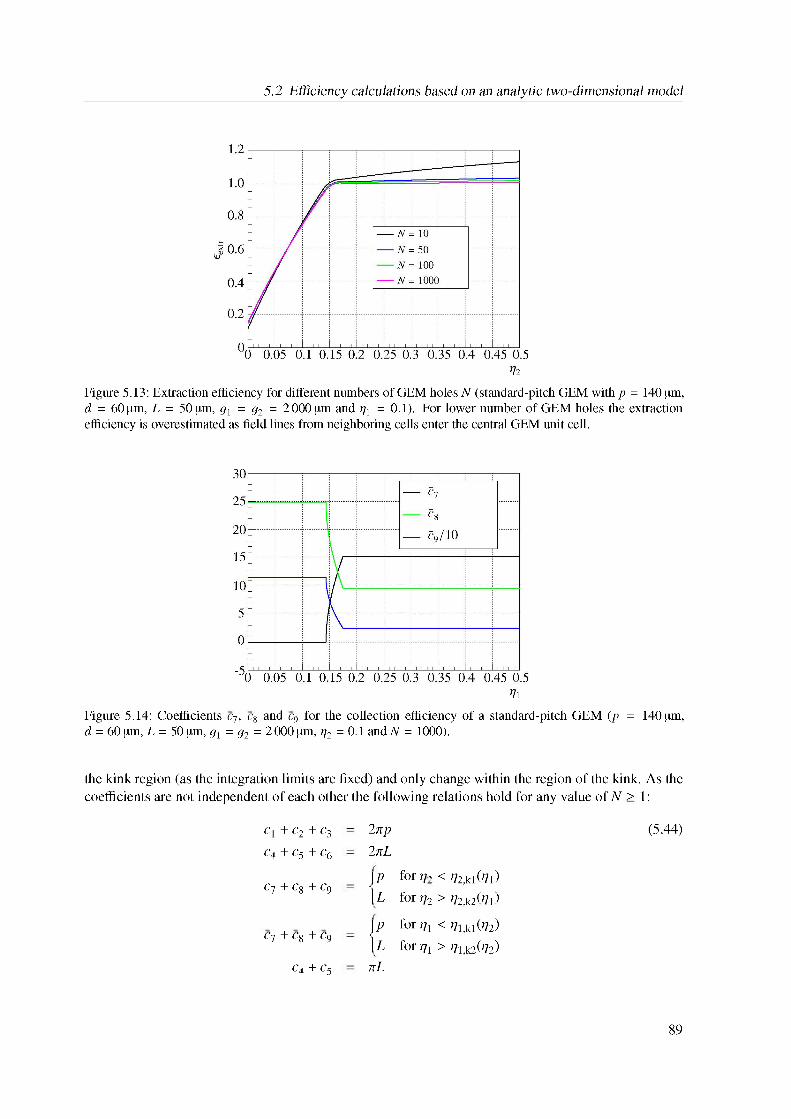
5.2 Efficiency calculations based on an analytic two-dimensional model
Figure 5.13: Extraction efficiency for different numbers of GEM holes N (standard-pitch GEM with p = 140 pm, d = 60 pm, L = 50 pm, g1 = g2 = 2000 pm and g1 = 0.1). For lower number of GEM holes the extraction efficiency is overestimated as field lines from neighboring cells enter the central GEM unit cell.
Figure 5.14: Coefficients c7, c8 and c9 for the collection efficiency of a standard-pitch GEM (p = 140 pm, d = 60pm, L = 50pm, g1 = g2 = 2000pm, g2 = 0.1 andN = 1000).
the kink region (as the integration limits are fixed) and only change within the region of the kink. As the coefficients are not independent of each other the following relations hold for any value of N > 1:
c1 + c2 + c3
c4 + c5 + c6
c7 + c8 + c9
c7 + c8 + c9
c4 + c5
2np2nL
p for //2 <^2,k1(^1) <
L for b2 >'/2.k2('/l’
p for ^1 <^1,k1(^2) <
L for ^1 > ^1,k2(^2)nL
(5.44)
89
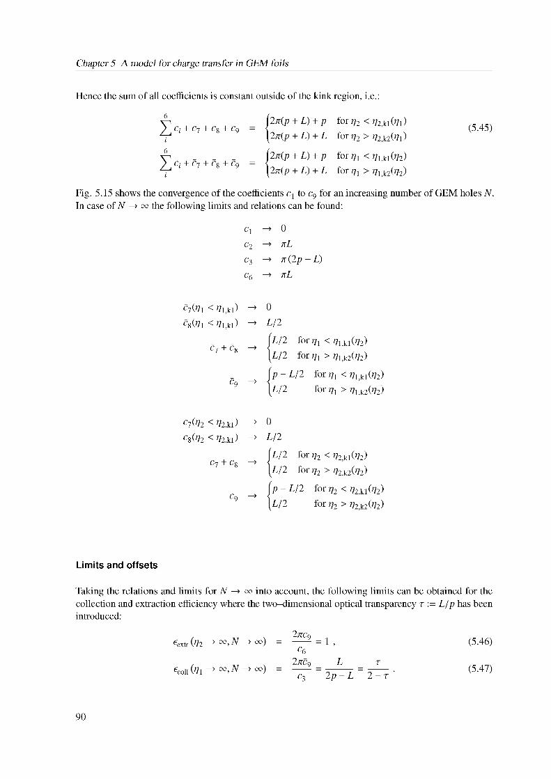
Chapter 5 A model for charge transfer in GEM foils
Hence the sum of all coefficients is constant outside of the kink region, i.e.:
6
X ci + c7 + c8 + c9 i6
X Ci + C7 + C8 + C9 i
2n(p + L) + p for p2 < P2.ki (Pi)2n(p + L) + L for p2 > P2.k2<Pi)
2n(p + L) + p for pi < ^ki(%)2n(p + L) + L for pi > Pi;k2(P2)
(5.45)
Fig. 5.i5 shows the convergence of the coefficients ci to C9 for an increasing number of GEM holes N. In case of N — 1 the following limits and relations can be found:
Ci - 0
C2 - -> nL
c3 - -> n (2p - L)
C6 - -> nL
C7 + C8 !
C9 !
c7(p2 < p2,ki) !
C8(P2 <P2,ki) !
c7 + c8 !
c9 !
C7(Pi < Pi.ki) !C8(Pi < Pi,ki) !
0L/2
L/2 for Pi < Pi.ki(P2)L/2 for Pi > Pi.k2(P2)
p ~ L/2 for Pi < Pi.ki(P2)L/2 for Pi > Pi.k2(P2)
0L/2
L/2 for P2 < P2.ki(P2)L/2 for P2 > P2.k2(P2)
p ~ L/2 for P2 <P2.ki(P2)L/2 for P2 > P2.k2(P2)
Limits and offsets
Taking the relations and limits for N — 1 into account, the following limits can be obtained for the collection and extraction efficiency where the two-dimensional optical transparency t := L/p has been introduced:
^extr (P2 ! 1; N ! 1Goll (Pi ! 1; N ! m)
2C1 = i .
c62nC9 L t
c3 2 p - L 2 - t '
(5.46)
(5.47)
90
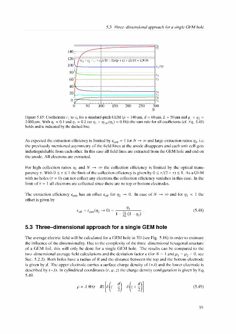
5.3 Three-dimensional approach for a single GEM hole
Figure 5.15: Coefficients c1 to c9 for a standard-pitch GEM (p = 140 pm, d = 60 pm, L = 50 pm and g1 = g2 = 2000 pm. With g1 = 0.1 and rp = 0.2 (so g2 > ^2;k2(^1) ~ 0.18)) the sum rule for all coefficients (cf. Eq. 5.45) holds and is indicated by the dashed line.
As expected the extraction efficiency is limited by eextr = 1 for N ! 1 and large extraction ratios ^2, i.e. the previously mentioned asymmetry of the field lines at the anode disappears and each unit cell gets indistinguishable from each other. In this case all field lines are extracted from the GEM hole and end on the anode. All electrons are extracted.
For high collection ratios p1 and N ! i the collection efficiency is limited by the optical transparency t. With 0 < t < 1 the limit of the collection efficiency is given by 0 < t/(2 - t) < 1. As a GEM with no holes (t = 0) can not collect any electrons the collection efficiency vanishes in this case. In the limit of t = 1 all electrons are collected since there are no top or bottom electrodes.
The extraction efficiency eextr has an offset eoff for p2 ! 0. In case of N ! i and for p1 < 1 the offset is given by
P1eoff = eextr(^2 ! 0) = ~ C^ 7 . (5.48)
1 - TL 0 - d11
5.3 Three-dimensional approach for a single GEM hole
The average electric field will be calculated for a GEM hole in 3D (see Fig. 5.16) in order to estimate the influence of the dimensionality. Due to the complexity of the three-dimensional hexagonal structure of a GEM foil, this will only be done for a single GEM hole. The results can be compared to the two-dimensional average field calculations and the deviation factor k (for N = 1 and g1 = g2 = 0, see Sec. 5.2.2). Both holes have a radius of R and the distance between the top and the bottom electrode is given by d. The upper electrode carries a surface charge density of (+fl) and the lower electrode is described by (-fl). In cylindrical coordinates (r, ', z) the charge density configuration is given by Eq. 5.49.
p = fl 0 (r - R) (5.49)
91
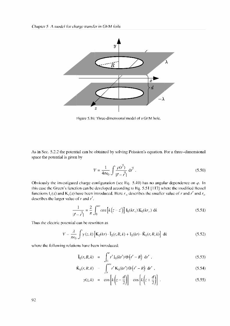
Chapter 5 A model for charge transfer in GEM foils
As in Sec. 5.2.2 the potential can be obtained by solving Poission’s equation. For a three-dimensional space the potential is given by
V =1 C P(~)
4^e0 \~ - r \r dr . (5.50)
Obviously the investigated charge configuration (see Eq. 5.49) has no angular dependence on '. In this case the Green’s function can be developed according to Eq. 5.51 [117] where the modified Bessel functions Iv(x) and Kv(x) have been introduced. Here r< describes the smaller value of r and r and r>
describes the larger value of r and r.
1 2 1 r / ai-------- — = cos k(z - z I0(kr<) K0(kr>) dk\ ~- r'\ n 0
Thus the electric potential can be rewritten as
V = — fy (z, k) [K0(kr) • Vr, R, k) + I0(kr) • K^, R, k)l dk ^0
where the following relations have been introduced:
I0(r, R, k) = j' r I0(kr) 0 (r' - R) dr' ,
1K0(r, R, k) = r K0(kr') 0 (r - r) dr' ,
[, d !#- cos k z + - .
(5.51)
(5.52)
(5.53)
(5.54)
(5.55)
~ r
y(z, k) = cos k
92
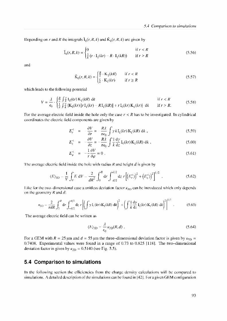
5.4 Comparison to simulations
Depending on r and R the integrals I0(r. R. k) and K0(r. R. k) are given by
~ 0 if r < R= >k (/, . ii(kr) _ r . I1(kR)) if r > R (5.56)
and
Ur.R.k) = [R'K1(‘R) ifr < R0 >r • K1(kr) if r > R (5.57)
which leads to the following potential
V = A >R Rk l0(kr)K1(kR) dk if r < Re0 ' U f I W [r I#r) - R I#R)] + r l0(kr)K#r)} dk if r > R. (5.58)
For the average electric field inside the hole only the case r < R has to be investigated. In cylindrical coordinates the electric field components are given by
The average electric field inside the hole with radius R and height d is given by
dV RA. CE< =----- =-------y k I1(kr)K1(kR) dk .
' dr ^e0 JE< = = Jid >0(kr)K1(kR)dk.
E<< = -1 @V = 0.r d<
(5.59)
(5.60)
(5.61)
1 C 2 CR fd/2 [/ < \2 i < X2]V2
<E>3D = VJVE dV = dRl^-dk1^ +E))| . (5.62)
Like for the two-dimensional case a unitless deviation factor k3D can be introduced which only depends on the geometry R and d:
The average electric field can be written as
*3D = ^2r £ dr ^\z r (Jy h(kr)K1(kR) dk) + (J k g ^(fcR) d^ . (5.63)
hEi3D = — k3D(R. d . e0
(5.64)
For a GEM with R = 25 pm and d = 55 pm the three-dimensional deviation factor is given by k3D = 0.7408. Experimental values were found in a range of 0.73 to 0.825 [118]. The two-dimensional deviation factor is given by k2D = 0.5140 (see Fig. 5.5).
5.4 Comparison to simulations
In the following section the efficiencies from the charge density calculations will be compared to simulations. A detailed description of the simulations can be found in [42]. For a given GEM configuration
93
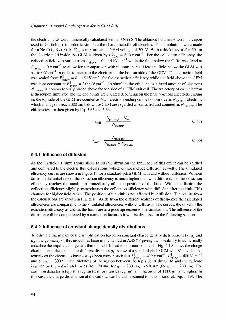
Chapter 5 A model for charge transfer in GEM foils
the electric fields were numerically calculated within ANSYS. The obtained field maps were thereupon used in Garfield++ in order to simulate the charge transfer efficiencies. The simulations were made for a Ne-CO2-N2 (90-10-5) gas mixture and a GEM voltage of 300 V. With a thickness of d = 50 pm the electric field inside the GEM is given by £’GEM = 60 kV cm-1. For the collection efficiency, the collection field was varied from T^ow = 0 _ 15 kV cm-1 while the field below the GEM was fixed at £’below = 0 V cm-1 to allow for a comparison with measurements. Here the field below the GEM was set to 0 V cm-1 in order to measure the electrons at the bottom side of the GEM. The extraction field was scaled from T^cw = 0 _ 15 kV cm-1 for the extraction efficiency while the field above the GEM was kept constant at T^we = 2 000 V cm-1. To simulate the efficiencies a fixed amount of electrons Nprimary is homogeneously placed above the top side of a GEM unit cell. The trajectory of each electron is thereupon simulated and the end points are counted depending on the final position: Electrons ending on the top side of the GEM are counted as Ntop, electrons ending on the bottom side as Nbottom. Electrons which manage to reach 300 pm below the GEM are regarded as extracted and counted as Ntransfer. The efficiencies are then given by Eq. 5.65 and 5.66.
Nprimary — Ntopecoll = ------N------------------ (5'65)
N primary
N_ = _____ 'transfer_____
Ntransfer + Nbottom(5.66)
5.4.1 Influence of diffusion
As the Garfield++ simulations allow to disable diffusion the influence of this effect can be studied and compared to the electric flux calculations (which do not include diffusion as well). The simulated efficiency curves are shown in Fig. 5.17 for a standard-pitch GEM with and without diffusion. Without diffusion the initial rise of the extraction efficiency is much higher than with diffusion, i.e. the extraction efficiency reaches the maximum immediately after the position of the kink. Without diffusion the collection efficiency slightly overestimates the collection efficiency with diffusion after the kink. This changes for higher field ratios. The position of the kink is not affected by diffusion. The results from the calculations are shown in Fig. 5.18. Aside from the different scalings of the //-axes the calculated efficiencies are comparable to the simulated efficiencies without diffusion. The curves, the offset of the extraction efficiency as well as the limits are in a good agreement to the simulations. The influence of the diffusion will be compensated by a correction factor as it will be discussed in the following sections.
5.4.2 Influence of constant charge density distributions
To estimate the impact of the simplification based on constant charge density distributions (ff, g1 and p2), the geometry of this model has been implemented in ANSYS giving the possibility to numerically calculate the required charge distributions which lead to constant potentials. Fig. 5.19 shows the charge distribution at the cathode for different distances g1 in case of a standard-pitch GEM with N = 2. The potentials on the electrodes have always been chosen such that TJbove = 400 V cm-1, Tbelow = 400 V cm-1
and Ggem = 300 V. The thickness of the region between the top side of the GEM and the cathode is given by (g1 - d)/2 and varies from 70 pm (for g1 = 200 pm) to 570 pm (for g1 = 1 200 pm). For common detector setups this region (drift or transfer region) is in the order of 1 000 pm and higher. In this case the charge distribution at the cathode can be well assumed to be constant (cf. Fig. 5.19). The
94
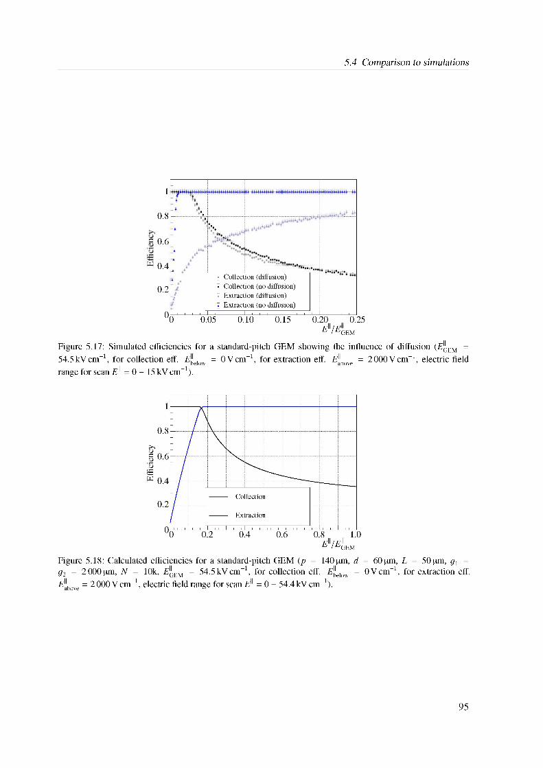
5.4 Comparison to simulations
c
1
0.8 —
0.6-
0.4-
0.2-
0,
III JCollection (diffusion)Collection (no diffusion)Extraction (diffusion)Extraction (no diffusion)
i —i—i—i—i—l i i i i l i i i i l i i I —I—i—i—i—i— 0 0.05 0.10 0.15 0.20 0.25.
E11 =Ej E = eGEM
Figure 5.17: Simulated efficiencies for a standard-pitch GEM showing the influence of diffusion (eGem = 54.5kVcm-1, for collection eff. Ebelow = 0Vcm-1, for extraction eff. E([bove = 2000Vcm-1, electric field range for scan E11 = 0 - 15 kV cm-1).
Figure 5.18: Calculated efficiencies for a standard-pitch GEM (p = 140 |im, d = 60 |im, L = 50 |im, g1 = g2 = 2000 |im, N = 10k, e{Lem = 54.5 kV cm-1, for collection eff. Ebelow = 0 V cm-1, for extraction eff. E(Jbove = 2 000 V cm-1, electric field range for scan E11 = 0 - 54.4 kV cm-1).
95
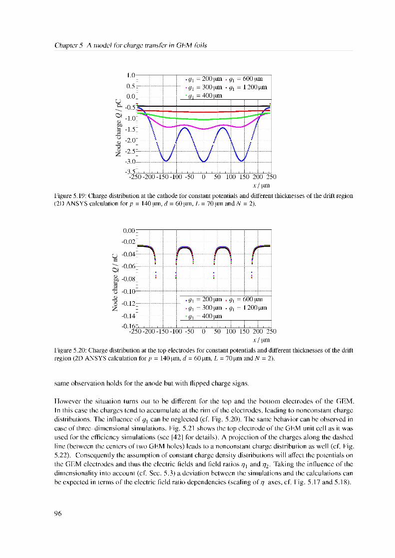
Chapter 5 A model for charge transfer in GEM foils
1.0R
0.0k
-0.5
-1.0k
-1.5?-2.0?
-2.5?-3.0-
0.5?
-3.5 -250-200-150-100 -50 0 50 100 150 200 250
x / pmFigure 5.19: Charge distribution at the cathode for constant potentials and different thicknesses of the drift region (2D ANSYS calculation for p = 140 pm, d = 60 pm, L = 70 pm and N = 2).
0.00
-0.02
-0.04
-0.06
-0.08
-0.10
-0.12
-0.14-0.16
-250-200-150-100 -50 0 50 100 150 200 250 x / pm
Figure 5.20: Charge distribution at the top electrodes for constant potentials and different thicknesses of the drift region (2D ANSYS calculation for p = 140 pm, d = 60 pm, L = 70 pm and N = 2).
same observation holds for the anode but with flipped charge signs.
However the situation turns out to be different for the top and the bottom electrodes of the GEM. In this case the charges tend to accumulate at the rim of the electrodes, leading to nonconstant charge distributions. The influence of g1 can be neglected (cf. Fig. 5.20). The same behavior can be observed in case of three-dimensional simulations. Fig. 5.21 shows the top electrode of the GEM unit cell as it was used for the efficiency simulations (see [42] for details). A projection of the charges along the dashed line (between the centers of two GEM holes) leads to a nonconstant charge distribution as well (cf. Fig. 5.22). Consequently the assumption of constant charge density distributions will affect the potentials on the GEM electrodes and thus the electric fields and field ratios p1 and ^2. Taking the influence of the dimensionality into account (cf. Sec. 5.3) a deviation between the simulations and the calculations can be expected in terms of the electric field ratio dependencies (scaling of ^-axes, cf. Fig. 5.17 and 5.18).
96
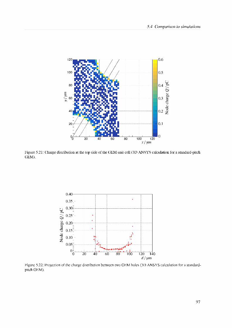
5.4 Comparison to simulations
Figure 5.21: Charge distribution at the top side of the GEM unit cell (3D ANSYS calculation for a standard-pitch GEM).
d / pm
Nod
e ch
arge
Q / p
C
pppp
pppp
O
'j, o 'JI
O 'JI
O 'JI
o
•
•» • >.
I4X'
I
0 20 40 60 80 100 120 140
Figure 5.22: Projection of the charge distribution between two GEM holes (3D ANSYS calculation for a standardpitch GEM).
97
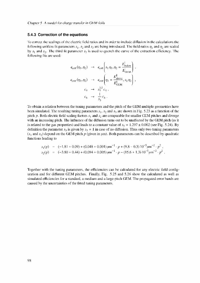
Chapter 5 A model for charge transfer in GEM foils
5.4.3 Correction of the equations
To correct the scalings of the electric field ratios and in order to include diffusion in the calculations the following unitless fit parameters 51, s2 and s3 are being introduced. The field ratios p1 and 12 are scaled by s1 and s2. The third fit parameter s3 is used to quench the curve of the extraction efficiency. The following fits are used:
o Fjj i„ EbelowGoll (11’12) --> Goll
belows1 11; 12 = ||rql< eGEM >
Gxtr (11;12) - Gxtr
0 /7jj 1above11 = || ; s212rql\ eGEM >
c4 -3 5 s3 C4 ;
c6 - ■* 7 c6.s3
To obtain a relation between the tuning parameters and the pitch of the GEM multiple geometries have been simulated. The resulting tuning parameters s1, s2 and s3 are shown in Fig. 5.23 as a function of the pitch p. Both electric field scaling factors s1 and s2 are comparable for smaller GEM pitches and diverge with an increasing pitch. The influence of the diffusion turns out to be unaffected by the GEM pitch (as it is related to the gas properties) and leads to a constant value of s3 = 1.297 ± 0.002 (see Fig. 5.24). By definition the parameter s3 is given by s3 = 1 in case of no diffusion. Thus only two tuning parameters (s1 and s2) depend on the GEM pitch p (given in pm). Both parameters can be described by quadratic functions leading to
s1(p) = (-1.81 ± 0.09) + (0.048 ± 0.001) pm"1 • p + (9.8 ± 0.3)10"5pm"2 • p2 ;s2(p) = (-3.80 ± 0.44) + (0.094 ± 0.005) pm"1 • p - (15.6 ± 1.3)10"5pm"2 • p2 .
Together with the tuning parameters, the efficiencies can be calculated for any electric field configuration and for different GEM pitches. Finally, Fig. 5.25 and 5.26 show the calculated as well as simulated efficiencies for a standard, a medium and a large-pitch GEM. The propagated error bands are caused by the uncertainties of the fitted tuning parameters.
98
5.4 Comparison to simulations
Figure 5.23: Tuning parameters 51, s2 and s3 for different GEM pitches (with d = 50 pm, L = 60 pm, g1 = g2 = 2110 pm and N = 200).
1.351------- ;--------11111-----------
1.34 E------ )-------(------- j------- j-------- j-------i-------- i--------1.33 k----- )------- (------- j------- j------- j------- ----------------1.32 r—1------ i------- j------- j-------- i-------i-------- i--------1.31k—|------ (------- 4------- k--|--(------- |------- |--------1.30 r----- i----- rit------t__-------k--------------1.29 k—’------- ------------------------------------------------
1.28 4-—)------ 4---~k------- 4------ i-------4---------------1.27 k----- )------- 1------- J------- J------- i------- 1-------- 1--------1.26 k----- i------- [------- i------- i------- i----------- 4-------- i--------
1.2550 100 150 200 250 300 350 400 450
p / pm
Figure 5.24: Detail view of tuning parameter s3 for different GEM pitches.
99
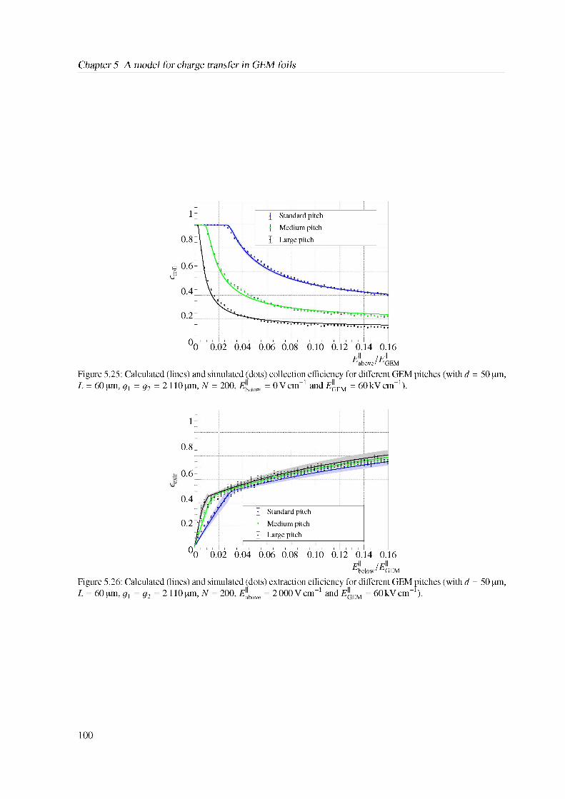
Chapter 5 A model for charge transfer in GEM foils
Figure 5.25: Calculated (lines) and simulated (dots) collection efficiency for different GEM pitches (with d = 50 um, L = 60 um, g1 = g2 = 2110 um, N = 200, E„e. w = 0Vcm-1 and eJLtEM = 60kVcm"1).
1
0.8:
0.2 ffl
0.4 L
0.6-
I Standard pitchI Medium pitch J Large pitch
Ebelow/EG EM
O i' i i i I i i i I i i i I i i i I i i i I i i i I i i i I i i i 00 0.02 0.04 0.06 0.08 0.10 0.12 0.14 0.16
Figure 5.26: Calculated (lines) and simulated (dots) extraction efficiency for different GEM pitches (with d = 50 um, L = 60 um, g = g2 = 2110 um, N = 200, Ebove = 2000Vcm"1 and e{Lem = 60kVcm"1).
100
CHAPTER 6
Model calculations
Fundamental properties of Micropattern Gaseous Detectors such as the energy resolution or the ion backflow depend highly on the charge transfer processes between the amplification stages. Based on the previous calculations of the efficiencies, expressions will be derived for the energy resolution and for the ion backflow in the following. The obtained model calculations will be compared to the measurements of the hybrid 2GEM-MM detector of Bonn (see Sec. 6.3) and Yale (see Sec. 6.4) as well as to the quadruple S-LP-LP-S stack of the ALICE TPC upgrade (see Sec. 6.5).
6.1 Energy-resolution model
The signal fluctuation and thus the energy resolution <r/p of a single GEM foil can be written as
£\ = IF + fM) y N~
(6.1)
and depends on the Fano factor F, the single gain fluctuation f and the number of collected electrons N~ (cf. Sec. 2.7). The contribution of electronic noise is neglected. Several statistical processes determine the energy resolution:
• The single electron gain can be described by a Polya distribution as introduced in Sec. 2.6.3. Within dedicated Garfield++ and ANSYS simulations [42], the single electron gain has been simulated for different GEM potentials and gas mixtures. The single electron gains can be seen in Fig. 6.1 in case of a standard-pitch GEM in Ne-CO2 (90-10) and for different GEM voltages. Polya distributions have been fitted to describe the data (cf. Sec. 2.6.3). In the limit of a low GEM potential, the Polya distribution approaches an exponential function (cf. Fig. 6.1(b)). The fitted Polya distributions allow to extract 6 and finally to obtain the single gain fluctuation f = 1/ (Q + 1). The resulting values for f are shown in Fig. 6.2 as a function of UGEM. The following empirical fit function has been introduced in order to describe the available data points
f (UGEM) = f0 + exp [(U0 “ UGEm) sU] (6.2)
where the limit for high GEM potentials is given by f0. The increase of the single gain fluctuation at lower GEM potentials is located at the potential U0. A further parameter sU has been introduced to allow for a scaling of the x-axis. A fit of f (UGEM) to the extracted single gain fluctuations gives f0 = 0.5720 ± 0.0015, U0 = (147 ± 3) V and sU = (0.051 ± 0.005)V-1. The curve f (UGEM) is
101
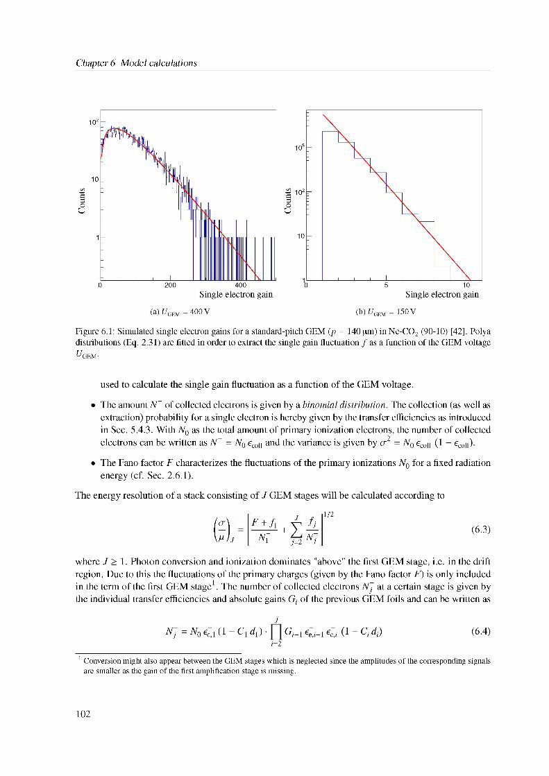
Chapter 6 Model calculations
Figure 6.1: Simulated single electron gains for a standard-pitch GEM (p = 140 |im) in Ne-CO2 (90-10) [42]. Polya distributions (Eq. 2.31) are fitted in order to extract the single gain fluctuation f as a function of the GEM voltage ^GEM.
used to calculate the single gain fluctuation as a function of the GEM voltage.
• The amount N~ of collected electrons is given by a binomial distribution. The collection (as well as extraction) probability for a single electron is hereby given by the transfer efficiencies as introduced in Sec. With N0 as the total amount of primary ionization electrons, the number of collected electrons can be written as N~ = N0 ecoll and the variance is given by a2 = N0 ecoll (1 - ecoll).
5.4.3.
• The Fano factor F characterizes the fluctuations of the primary ionizations N0 for a fixed radiation energy (cf. Sec. . 2.6.1)
The energy resolution of a stack consisting of J GEM stages will be calculated according to
F + f1
Nf
31=2
(6.3)V1 fj+§ Ni
where J > 1. Photon conversion and ionization dominates "above" the first GEM stage, i.e. in the drift region. Due to this the fluctuations of the primary charges (given by the Fano factor F) is only included in the term of the first GEM stage1. The number of collected electrons NJ at a certain stage is given by the individual transfer efficiencies and absolute gains Gi of the previous GEM foils and can be written as
1 Conversion might also appear between the GEM stages which is neglected since the amplitudes of the corresponding signals are smaller as the gain of the first amplification stage is missing.
j
Nj = N0 6j,)1 C1 - C1 d1) • Gi_1 ee,i-1 6C,i C1 “ Ci di) (6.4)i=2
102
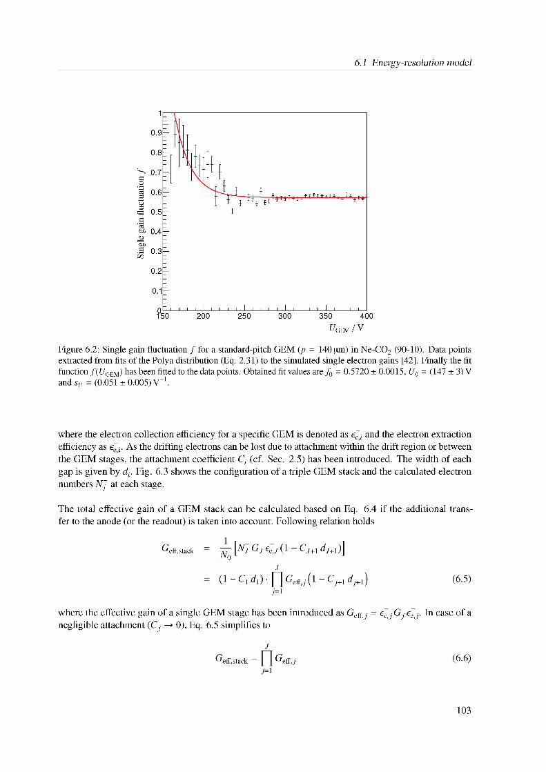
6.1 Energy-resolution model
Figure 6.2: Single gain fluctuation f for a standard-pitch GEM (p = 140 |im) in Ne-CO2 (90-10). Data points extracted from fits of the Polya distribution (Eq. 2.31) to the simulated single electron gains [42]. Finally the fit function f (UGEM) has been fitted to the data points. Obtained fit values are f0 = 0.5720 ± 0.0015, U0 = (147 ± 3) V and sU = (0.051 ± 0.005)V-1.
where the electron collection efficiency for a specific GEM is denoted as e~; and the electron extraction efficiency as e~;. As the drifting electrons can be lost due to attachment within the drift region or between the GEM stages, the attachment coefficient C; (cf. Sec. 2.5) has been introduced. The width of each gap is given by d;. Fig. 6.3 shows the configuration of a triple GEM stack and the calculated electron numbers NJ at each stage.
The total effective gain of a GEM stack can be calculated based on Eq. 6.4 if the additional transfer to the anode (or the readout) is taken into account. Following relation holds
Geff, stack NJ lNj Gj e&,J ^1 “ Cj+1 dJ+1)]J
(1 - C1 d1) J] Geff,j (1 - Cj+1 dj+1) j=1
(6.5)
where the effective gain of a single GEM stage has been introduced as Geff,j = ecj Gj ee,j. In case of a negligible attachment (Cj ! 0), Eq. 6.5 simplifies to
J
Geff stack = Geff j (6.6)
103
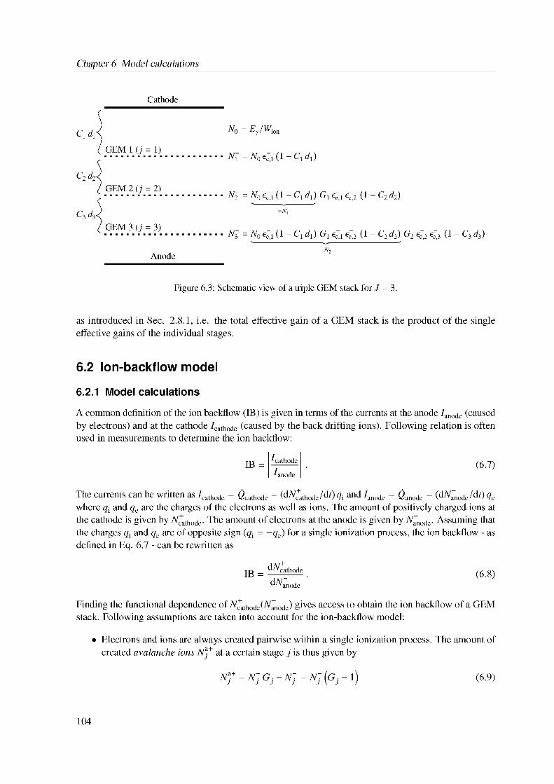
Chapter 6 Model calculations
Cathode
C1 d1
GEM 1 (j = 1)
No = E7/Wion
N1 = No £c,1 C1 _ C1 d1)
C2 d2'GEM 2 (j = 2)
N2 = N0 £c,1 C1 “ C1 d1) G1 £e,1 £c,2 C1 “ C2 d2)
C3 d3
^^z=N1
GEM 3 (j = 3)N3- = No e“1 (1 - C1 dj G1 c~1 c~2 (1 - C2 d^ G2 £~2 <3 (1 - C3 dj)
Anode^{^“=N2
Figure 6.3: Schematic view of a triple GEM stack for J = 3.
as introduced in Sec. 2.8.1, i.e. the total effective gain of a GEM stack is the product of the single effective gains of the individual stages.
6.2 Ion-backflow model
6.2.1 Model calculations
A common definition of the ion backflow (IB) is given in terms of the currents at the anode /anode (caused by electrons) and at the cathode /cathode (caused by the back drifting ions). Following relation is often used in measurements to determine the ion backflow:
IB = ^cathode
danode(6.7)
The Current can be written as /cathode = kathode = (dNc+athode=dt) di and 4node = Ganode = (dNanode=dt) de where qi and qe are the charges of the electrons as well as ions. The amount of positively charged ions at the cathode is given by Nc~athode. The amount of electrons at the anode is given by Na"node. Assuming that the charges qi and qe are of opposite sign (qi = -qe) for a single ionization process, the ion backflow - as defined in Eq. 6.7 - can be rewritten as
IB = dNcathode
dNanode(6.8)
Finding the functional dependence of N+athode(Nanode) gives access to obtain the ion backflow of a GEM stack. Following assumptions are taken into account for the ion-backflow model:
• Electrons and ions are always created pairwise within a single ionization process. The amount of created avalanche ions Nj+ at a certain stage j is thus given by
N -= NJGj - Nj = N g - (6.9)
104
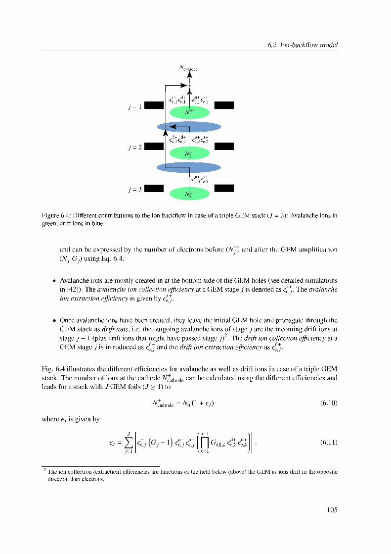
6.2 Ion-backflow model
N+ cathode
j = 1
j =
j = 3
,e a+ e a+ ec,1ee,1,e d+P d+ ec,1 ee,1
,e a+ e a+ ec,2ee,2
N
,e d+f d+ ec,2 ee,2
,e a+ e a+ ec,3ee,3
N2a+
N3a+
Figure 6.4: Different contributions to the ion backflow in case of a triple GEM stack (J = 3): Avalanche ions in green, drift ions in blue.
and can be expressed by the number of electrons before (Nj) and after the GEM amplification (NJ Gj) using Eq. 6.4.
• Avalanche ions are mostly created in at the bottom side of the GEM holes (see detailed simulations in [42]). The avalanche ion collection efficiency at a GEM stage j is denoted as e^-. The avalanche ion extraction efficiency is given by eJJ.
• Once avalanche ions have been created, they leave the initial GEM hole and propagate through the GEM stack as drift ions, i.e. the outgoing avalanche ions of stage j are the incoming drift ions at stage j - 1 (plus drift ions that might have passed stage j)2. The drift ion collection efficiency at a GEM stage j is introduced as ed+ and the drift ion extraction efficiency as ed+.
2 The ion collection (extraction) efficiencies are functions of the field below (above) the GEM as ions drift in the opposite direction than electrons.
Fig. 6.4 illustrates the different efficiencies for avalanche as well as drift ions in case of a triple GEM stack. The number of ions at the cathode N+athode can be calculated using the different efficiencies and leads for a stack with J GEM foils (J > 1) to
Ncathode = N0 C1 + eJ) (6.10)
where eJ is given by
eJ =j=1
a+ a+ ec, j ce, j
0 j-1 1n,-. d+ d+Geff,k eck ee,k
\k=1 ,(6.11)
J
105
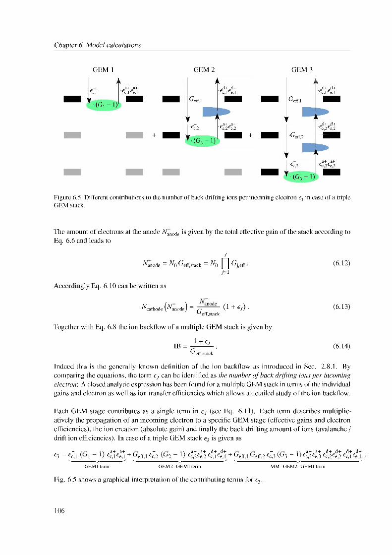
Chapter 6 Model calculations
GEM 1 GEM 3
Cc,1V-G - 1)
,ca+ ca+ ec,1ce,1
GEM 2
'ec,3
./+/+ ec,1ce,1
'ec,2ee,2G
■ G - 1)
,ca+ Ca+ ec,3ee,3
Figure 6.5: Different contributions to the number of back drifting ions per incoming electron c3 in case of a triple GEM stack.
The amount of electrons at the anode Nanode is given by the total effective gain of the stack according to Eq. 6.6 and leads to
j
Nnode = No Geff,stack = N) [J Gj,eff • (6.12)
Accordingly Eq. 6.10 can be written as
Cthode (N^de) = (1 + Cj) . (6.13)Geff,stack
Together with Eq. 6.8 the ion backflow of a multiple GEM stack is given by
1 + Ct IB = ------- J- . (6.14)Geff,stack
Indeed this is the generally known definition of the ion backflow as introduced in Sec. 2.8.1. By comparing the equations, the term cj can be identified as the number of back drifting ions per incoming electron: A closed analytic expression has been found for a multiple GEM stack in terms of the individual gains and electron as well as ion transfer efficiencies which allows a detailed study of the ion backflow.
Each GEM stage contributes as a single term in ct (see Eq. 6.11). Each term describes multiplicatively the propagation of an incoming electron to a specific GEM stage (effective gains and electron efficiencies), the ion creation (absolute gain) and finally the back drifting amount of ions (avalanche / drift ion efficiencies). In case of a triple GEM stack c3 is given as
_ - / ) a+ a+ — / ) a+ a+ d+ d+ — a+ a+ d+ d+ d+ d+ c3 = Cc,1 G1 “ 1 cc,1ce,1 + Geff,1 Cc,2 G2 “ 1 cc,2ce,2 Cc,1 ce,1 + Geff,1 Geff,2 Cc,3 (g3 “ 1) cc,3ce,3 Cc,2ce,2 Cc,1 ce,1 .
| {Z } | {Z } | {Z }GEM1 term GEM2-GEM1 term MM-GEM2-GEM1 term
Fig. 6.5 shows a graphical interpretation of the contributing terms for c3.
106
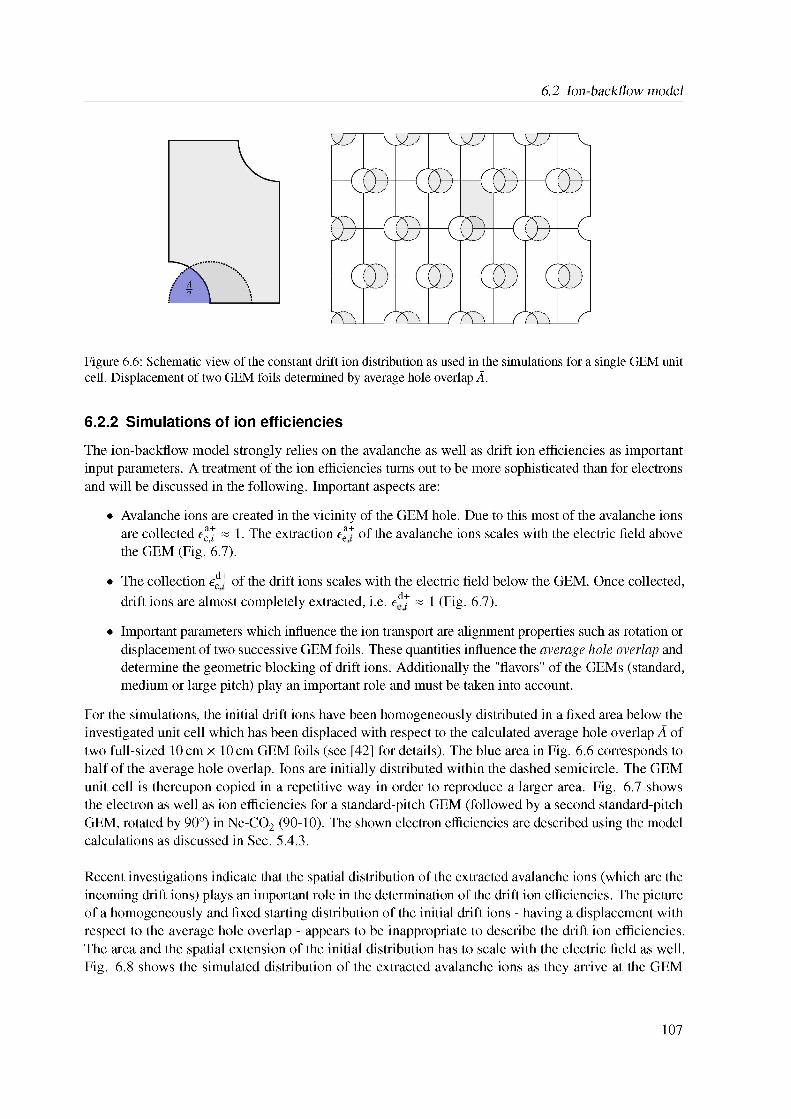
6.2 Ion-backflow model
Figure 6.6: Schematic view of the constant drift ion distribution as used in the simulations for a single GEM unit 11 -r^ • 1 . c . ir i' • 1 1 • 1 1 11 1 Tcell. Displacement of two GEM foils determined by average hole overlap A.
6.2.2 Simulations of ion efficiencies
The ion-backflow model strongly relies on the avalanche as well as drift ion efficiencies as important input parameters. A treatment of the ion efficiencies turns out to be more sophisticated than for electrons and will be discussed in the following. Important aspects are:
• Avalanche ions are created in the vicinity of the GEM hole. Due to this most of the avalanche ions are collected e^ « 1. The extraction 6^+ of the avalanche ions scales with the electric field above the GEM (Fig. . 6.7)
• The collection e£+ of the drift ions scales with the electric field below the GEM. Once collected, drift ions are almost completely extracted, i.e. 6d+ « 1 (Fig. . 6.7)
• Important parameters which influence the ion transport are alignment properties such as rotation or displacement of two successive GEM foils. These quantities influence the average hole overlap and determine the geometric blocking of drift ions. Additionally the "flavors" of the GEMs (standard, medium or large pitch) play an important role and must be taken into account.
For the simulations, the initial drift ions have been homogeneously distributed in a fixed area below the investigated unit cell which has been displaced with respect to the calculated average hole overlap A of two full-sized 10 cm x 10 cm GEM foils (see [42] for details). The blue area in Fig. 6.6 corresponds to half of the average hole overlap. Ions are initially distributed within the dashed semicircle. The GEM unit cell is thereupon copied in a repetitive way in order to reproduce a larger area. Fig. 6.7 shows the electron as well as ion efficiencies for a standard-pitch GEM (followed by a second standard-pitch GEM, rotated by 90°) in Ne-CO2 (90-10). The shown electron efficiencies are described using the model calculations as discussed in Sec. 5.4.3.
Recent investigations indicate that the spatial distribution of the extracted avalanche ions (which are the incoming drift ions) plays an important role in the determination of the drift ion efficiencies. The picture of a homogeneously and fixed starting distribution of the initial drift ions - having a displacement with respect to the average hole overlap - appears to be inappropriate to describe the drift ion efficiencies. The area and the spatial extension of the initial distribution has to scale with the electric field as well. Fig. 6.8 shows the simulated distribution of the extracted avalanche ions as they arrive at the GEM
107
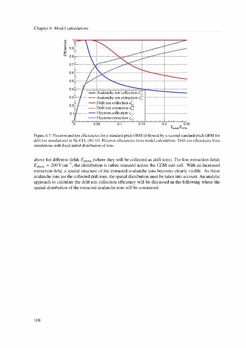
Chapter 6 Model calculations
Figure 6.7: Electron and ion efficiencies for a standard-pitch GEM (followed by a second standard-pitch GEM for drift ion simulations) in Ne-CO2 (90-10). Electron efficiencies from model calculations. Drift ion efficiencies from simulations with fixed initial distribution of ions.
above for different fields Eabove (where they will be collected as drift ions). For low extraction fields £’above ~ 200 Vcm-1, the distribution is rather smeared across the GEM unit cell. With an increased extraction field, a spatial structure of the extracted avalanche ions becomes clearly visible. As these avalanche ions are the collected drift ions, the spatial distribution must be taken into account. An analytic approach to calculate the drift ion collection efficiency will be discussed in the following where the spatial distribution of the extracted avalanche ions will be considered.
108
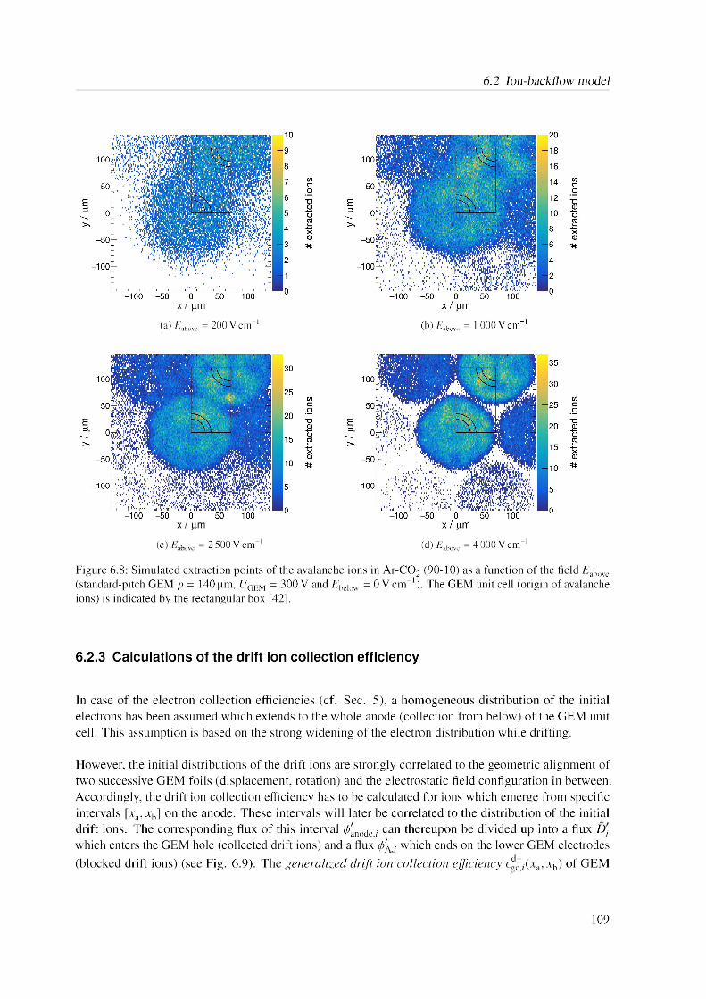
6.2 Ion-backflow model
x I pm
(a) EabOve = 200 V cm-1 (b) Ebnw = 1 000 V cm
(c) I.. = 2 500 V cm-1 (d) Eabove = 4 000 V cm-1Figure 6.8: Simulated extraction points of the avalanche ions in Ar-CO2 (90-10) as a function of the field Eabove
(standard-pitch GEM p = 140 pm, [7GEM = 300 V and Ebelow = 0Vcm“1). The GEM unit cell (origin of avalanche ions) is indicated by the rectangular box [42].
6.2.3 Calculations of the drift ion collection efficiency
In case of the electron collection efficiencies (cf. Sec. 5), a homogeneous distribution of the initial electrons has been assumed which extends to the whole anode (collection from below) of the GEM unit cell. This assumption is based on the strong widening of the electron distribution while drifting.
However, the initial distributions of the drift ions are strongly correlated to the geometric alignment of two successive GEM foils (displacement, rotation) and the electrostatic field configuration in between. Accordingly, the drift ion collection efficiency has to be calculated for ions which emerge from specific intervals [xa, xb] on the anode. These intervals will later be correlated to the distribution of the initial drift ions. The corresponding flux of this interval ^anode>i can thereupon be divided up into a flux D0
which enters the GEM hole (collected drift ions) and a flux ^A i which ends on the lower GEM electrodes (blocked drift ions) (see Fig. 6.9). The generalized drift ion collection efficiency 6^+(xa, xb) of GEM
109
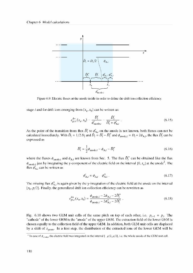
Chapter 6 Model calculations
Figure 6.9: Electric fluxes at the anode inside in order to define the drift ion collection efficiency.
stage i and for drift ions emerging from [xa, xb] can be written as:
A (x xj = -D- = -* — gc,i xa’ xb 0 0 0 •
3 In case of ^.inod„,i the electric field was integrated on the interval [-p/2, p/2], i.e. the whole anode of the GEM unit cell.
^anode.i Di + 0A,i(6.15)
An ♦ . c n . f n r\f < if n i • . i inn . iAs the point of the transition from flux D0 to ^>A i on the anode is not known, both fluxes can not be calculated immediately. With Di = 1/2 Di and Di = D0 + D0 and 0anode;i = Di + 20A;i, the flux D 0 can be expressed as
1Di = 2 ^anode.i 0A,i Di (6.16)
inn i ii i c nm n r\f f i i . i i’i n nwhere the fluxes 0anode;i and 0A;i are known from Sec. 5. The flux D0 can be obtained like the flux 0anode;i just by integrating the y-component of the electric field on the interval [0, xa] at the anode3. The flux <p'A;i can be written as
^A,i = ^A,i - ^A,i • (6.17)
The missing flux $A,i is again given by the y-integration of the electric field at the anode on the interval [xb, p/2]. Finally, the generalized drift ion collection efficiency can be rewritten as
d+ egc,i (W; xb)
0anode,i 2^A,i 2Di<^anode,i " 2<P'A,i ~ 2Di
(6.18)
Fig. 6.10 shows two GEM unit cells of the same pitch on top of each other, i.e. pi+1 = pi. The "cathode" of the lower GEM is the "anode" of the upper GEM. The extraction field of the lower GEM is chosen equally to the collection field of the upper GEM. In addition, both GEM unit cells are displaced by a shift of xgeom. In a first step, the distribution of the extracted ions of the lower GEM will be
110
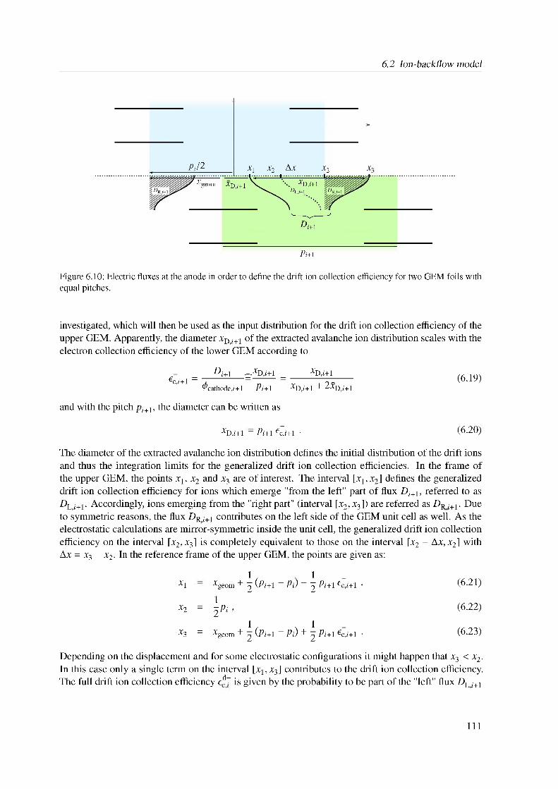
6.2 Ion-backflow model
Pi/2
geomx1
xD,i+1xD,i+1
x2 - A x
Pi+1
Figure 6.10: Electric fluxes at the anode in order to define the drift ion collection efficiency for two GEM foils with equal pitches.
investigated, which will then be used as the input distribution for the drift ion collection efficiency of the upper GEM. Apparently, the diameter xD,i+1 of the extracted avalanche ion distribution scales with the electron collection efficiency of the lower GEM according to
ec,i+1 -Di+1 — xD,i+1
0cathode,i+1 Pi+1
xD,i+1
xD,i+1 + 2xD,i+1(6.19)
and with the pitch pi+1, the diameter can be written as
xD,i+1 - pi+1 ec,i+1 ■ (6.20)
The diameter of the extracted avalanche ion distribution defines the initial distribution of the drift ions and thus the integration limits for the generalized drift ion collection efficiencies. In the frame of the upper GEM, the points x1, x2 and x3 are of interest. The interval [x1, x2] defines the generalized drift ion collection efficiency for ions which emerge "from the left" part of flux Di+1, referred to as DL,i+1. Accordingly, ions emerging from the "right part" (interval [x2, x3]) are referred as DRi+1. Due to symmetric reasons, the flux DR,i+1 contributes on the left side of the GEM unit cell as well. As the electrostatic calculations are mirror-symmetric inside the unit cell, the generalized drift ion collection efficiency on the interval [x2, x3] is completely equivalent to those on the interval [x2 - Ax, x2] with Ax - x3 - x2. In the reference frame of the upper GEM, the points are given as:
1 1x1 xgeom + 2 (Pi+1 - Pi) - ^ Pi+1 ec,i+1, (6.21)
x2 1- 2 Pi, (6.22)
x3 = xgeom + 11 f2 (Pi+1 - Pi)
1+ 2 Pi+1 ec,i+1 ■ (6.23)
Depending on the displacement and for some electrostatic configurations it might happen that x3 < x2. In this case only a single term on the interval [x1, x3] contributes to the drift ion collection efficiency. The full drift ion collection efficiency ed+ is given by the probability to be part of the "left" flux DLi+1
111
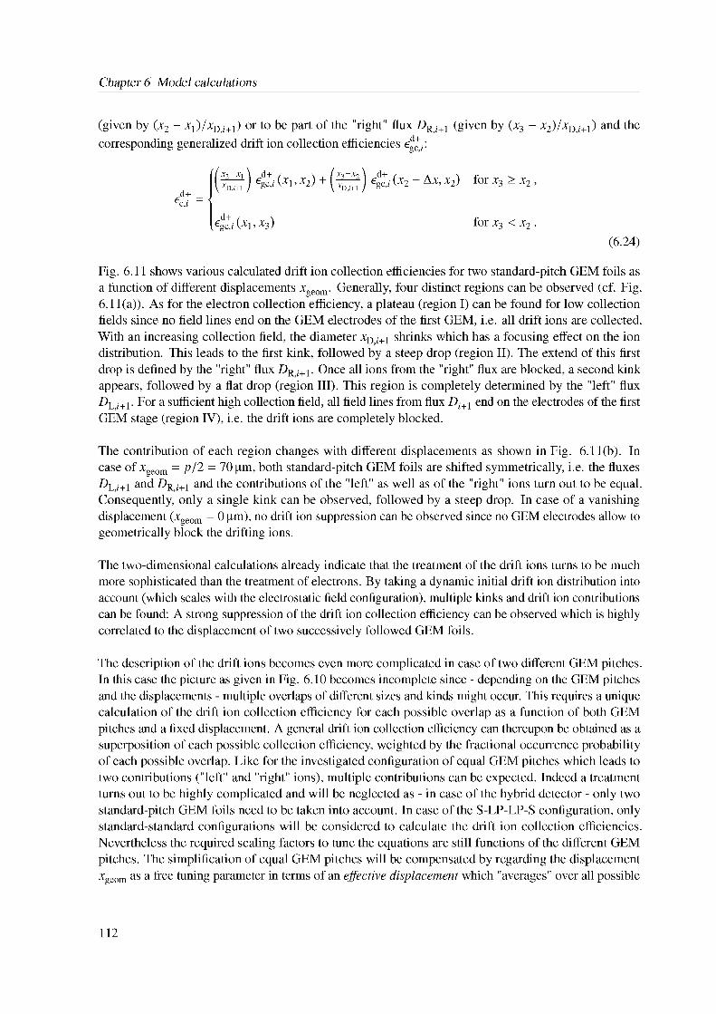
Chapter 6 Model calculations
(given by (x2 - x1)/xDi+1) or to be part of the "right" flux DR,i+1 (given by (x3 - x2)/xD,i+1) and the corresponding generalized drift ion collection efficiencies eg^p.
d+cc,i
(x2~xi \ d+ z X (x3 x2 \ d+ ZrxD,i+1 ('X1 ’ 2 + x D J egc, AX2
,4+i (xi, x3)
Ax, x2) for x3 > x2 ,
for x3 < x2 .
(6.24)
Fig. 6.11 shows various calculated drift ion collection efficiencies for two standard-pitch GEM foils as a function of different displacements xgeom. Generally, four distinct regions can be observed (cf. Fig. 6.11(a)). As for the electron collection efficiency, a plateau (region I) can be found for low collection fields since no field lines end on the GEM electrodes of the first GEM, i.e. all drift ions are collected. With an increasing collection field, the diameter xD,i+1 shrinks which has a focusing effect on the ion distribution. This leads to the first kink, followed by a steep drop (region II). The extend of this first drop is defined by the "right" flux DR,i+1. Once all ions from the "right" flux are blocked, a second kink appears, followed by a flat drop (region III). This region is completely determined by the "left" flux DL,i+1. For a sufficient high collection field, all field lines from flux Di+1 end on the electrodes of the first GEM stage (region IV), i.e. the drift ions are completely blocked.
The contribution of each region changes with different displacements as shown in Fig. 6.11(b). In case of xgeom = p/2 = 70 pm, both standard-pitch GEM foils are shifted symmetrically, i.e. the fluxes DL,i+1 and DR,i+1 and the contributions of the "left" as well as of the "right" ions turn out to be equal. Consequently, only a single kink can be observed, followed by a steep drop. In case of a vanishing displacement (xgeom = 0 pm), no drift ion suppression can be observed since no GEM electrodes allow to geometrically block the drifting ions.
The two-dimensional calculations already indicate that the treatment of the drift ions turns to be much more sophisticated than the treatment of electrons. By taking a dynamic initial drift ion distribution into account (which scales with the electrostatic field configuration), multiple kinks and drift ion contributions can be found: A strong suppression of the drift ion collection efficiency can be observed which is highly correlated to the displacement of two successively followed GEM foils.
The description of the drift ions becomes even more complicated in case of two different GEM pitches. In this case the picture as given in Fig. 6.10 becomes incomplete since - depending on the GEM pitches and the displacements - multiple overlaps of different sizes and kinds might occur. This requires a unique calculation of the drift ion collection efficiency for each possible overlap as a function of both GEM pitches and a fixed displacement. A general drift ion collection efficiency can thereupon be obtained as a superposition of each possible collection efficiency, weighted by the fractional occurrence probability of each possible overlap. Like for the investigated configuration of equal GEM pitches which leads to two contributions ("left" and "right" ions), multiple contributions can be expected. Indeed a treatment turns out to be highly complicated and will be neglected as - in case of the hybrid detector - only two standard-pitch GEM foils need to be taken into account. In case of the S-LP-LP-S configuration, only standard-standard configurations will be considered to calculate the drift ion collection efficiencies. Nevertheless the required scaling factors to tune the equations are still functions of the different GEM pitches. The simplification of equal GEM pitches will be compensated by regarding the displacement xgeom as a free tuning parameter in terms of an effective displacement which "averages" over all possible
112
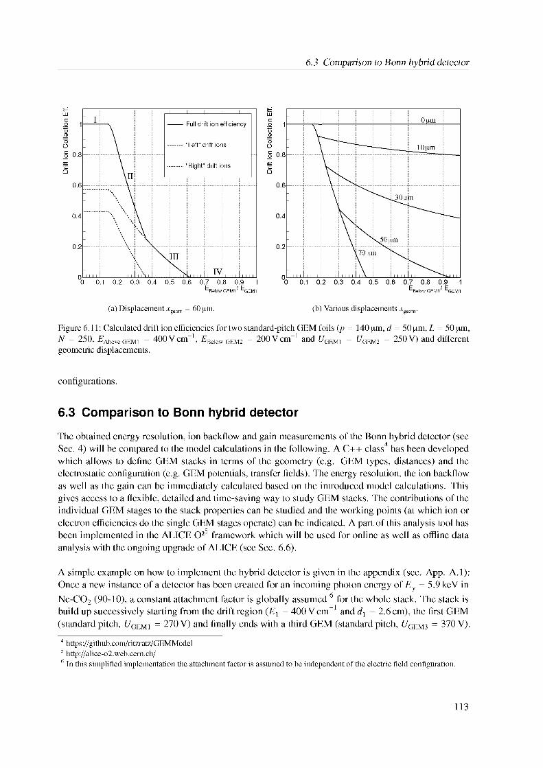
6.3 Comparison to Bonn hybrid detector
(a) Displacement xgeom = 60 pm. (b) Various displacements xgeom.
Figure 6.11: Calculated drift ion efficiencies for two standard-pitch GEM foils (p = 140 pm, d = 50 pm, L = 50 pm, N = 250, E Above GEM1 = 400 V cm \ EBelow GEM2 = 200 V cm 1 and ^GEM1 = EGEM2 = 250 V) and different geometric displacements.
configurations.
6.3 Comparison to Bonn hybrid detector
The obtained energy resolution, ion backflow and gain measurements of the Bonn hybrid detector (see Sec. 4) will be compared to the model calculations in the following. A C++ class4 5 has been developed which allows to define GEM stacks in terms of the geometry (e.g. GEM types, distances) and the electrostatic configuration (e.g. GEM potentials, transfer fields). The energy resolution, the ion backflow as well as the gain can be immediately calculated based on the introduced model calculations. This gives access to a flexible, detailed and time-saving way to study GEM stacks. The contributions of the individual GEM stages to the stack properties can be studied and the working points (at which ion or electron efficiencies do the single GEM stages operate) can be indicated. A part of this analysis tool has been implemented in the ALICE O25 framework which will be used for online as well as offline data analysis with the ongoing upgrade of ALICE (see Sec. 6.6).
4 https://github.com/ritzratz/GEMModel5 http://alice-o2.web.cern.ch/6 In this simplified implementation the attachment factor is assumed to be independent of the electric field configuration.
A simple example on how to implement the hybrid detector is given in the appendix (see. App. A.1): Once a new instance of a detector has been created for an incoming photon energy of E? = 5.9 keV in Ne-CO2 (90-10), a constant attachment factor is globally assumed 6 for the whole stack. The stack is build up successively starting from the drift region (E1 = 400 V cm-1 and d1 = 2.6 cm), the first GEM (standard pitch, f/GEM1 = 270 V) and finally ends with a third GEM (standard pitch, f/GEM3 = 370 V).
113
Chapter 6 Model calculations
The last stage should contribute as a Micromegas which is realized by tuning the properties of the last "GEM": The gain curve is overwritten by the measured curve of the Micromegas (see Sec. 4.3.1). As a Micromegas is almost opaque for ions and transparent for electrons (see Sec. 2.8.2) the efficiencies are set to 6^,3 = 0.99, eea,+ = 0.01 for avalanche ions (there are not drift ions) and e~3 = 0-99, e~3 = 1.00 for electrons.
The calculated energy resolution as well as ion backflow values can be seen in Fig. 6.12 for different TF2 scans. The total effective gain of the stack is shown in Fig. 6.13. Generally, the measurements are in a good agreement to the model calculations. Only the calculated gain curve for ETF2 = 400 V cm-1
shows a linear trend which can not be seen in case of the measured data points: For lower GEM1 potential, the effective gain is overestimated. In case of higher GEM1 potentials, the effective gain is underestimated. This trend will be discussed in detail in case of the Yale hybrid detector (see Sec. 6.4).
The error bands of the ion backflow calculations are based on an error propagation of Eq. 6.14. The errors of the electron efficiencies are given by the accuracy of the fits, i.e. by the tuning factors 51, s2 and s3. The simulated avalanche ion efficiencies (cf. Fig. 6.7) are fitted by higher polynomial functions. Accordingly, the uncertainties of the polynomial coefficients determine the error of the avalanche ion efficiencies. As the drift ion collection efficiencies are calculated using the tuning factors s1 for two successive GEM foils (cf. Sec. 6.2.3), these factors determine the errors. The drift ion extraction efficiency is assumed to be constant ed+ = 1 for the calculations and no error is assumed (Aed+ = 0). The errors of the gains are given by the uncertainties of the fitted exponential functions to the simulated gain curves.
The propagation of n electrons between two amplification stages can be described by a binomial distribution where the probability p is given by the transfer efficiencies and the attachment coefficients. At each stage, np electrons can be expected (cf. Sec. 6.1) and the variance is given by (ANf) = np(1 - p). In the following no errors are assumed for the attachment coefficient as well as for the Fano factor. As the error of the single gain fluctuation turns out to be asymmetric (AfHi and AfLo, see Fig. 6.2), the following equations are used in order to estimate the lower / upper limit of the energy resolution
F + f1 + Af1,Hi f2 + Af2,Hi---------------------- + ---------------- + ... ,
N1" - ANT N2 - AN2
F + f - Af1,Lo
N1" + ANT
f2 Af2,Lo+------Z---------- —
N + AN2
(6.25)
(6.26)+...
The model calculations allow a detailed study of the dynamics within a GEM stack and to analyze the influence of each stage to the whole setup. Fig. 6.14(a) shows the individual GEM/MM contributions to the total effective gain of the detector for each data point in case of ETF2 = 400 V cm-1: As the total effective gain was kept approximately at 2 000 during the GEM1-MM scans, the calculated gain can be expected to be constant too (see black bars). The effective gain contribution of the first GEM increases with an increasing GEM1 potential (red bars), while the effective gain of the Micromegas decreases (green bars). Most of the gain is contributed by the Micromegas.
The contributions of the single terms for e3 are shown in Fig. 6.14(b) for each data point within the scans (low GEM1 potentials to high GEM1 potentials). With an increasing GEM1 potential, more
114
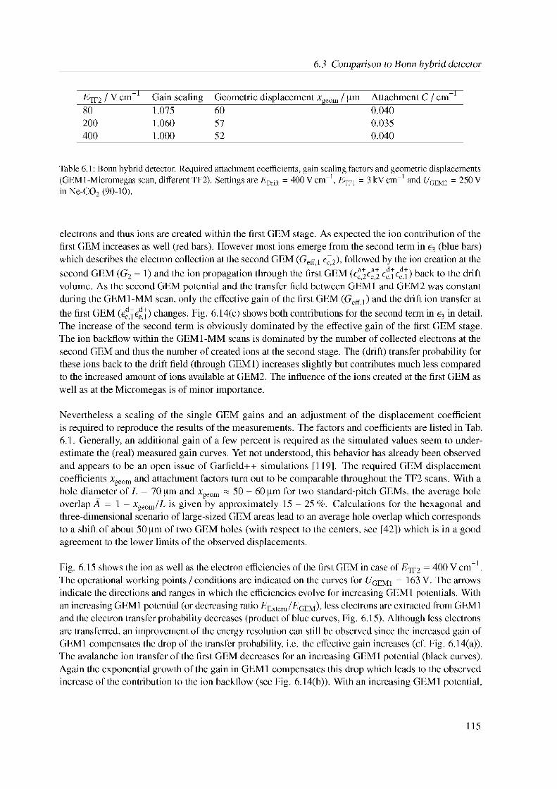
6.3 Comparison to Bonn hybrid detector
Table 6.1: Bonn hybrid detector. Required attachment coefficients, gain scaling factors and geometric displacements (GEMl-Micromegas scan, different TF2). Settings are EDrift = 400 Vcm-1, ETF1 = 3kVcm-1 and GGEM2 = 250 V in Ne-CO2 (90-10).
ETF2 / V cm 1 Gain scaling Geometric displacement xgeom / um Attachment C / cm 1
80 1.075 60 0.040200 1.060 57 0.035400 1.000 52 0.040
electrons and thus ions are created within the first GEM stage. As expected the ion contribution of the first GEM increases as well (red bars). However most ions emerge from the second term in e3 (blue bars) which describes the electron collection at the second GEM (Geff;1 e~2), followed by the ion creation at the second GEM (G2 - 1) and the ion propagation through the first GEM (cc'.2ee.2 ec,1 ee,1) back to the drift volume. As the second GEM potential and the transfer field between GEM1 and GEM2 was constant during the GEM1-MM scan, only the effective gain of the first GEM (Geff;1) and the drift ion transfer at the first GEM (ed1‘e^) changes. Fig. 6.14(c) shows both contributions for the second term in e3 in detail. The increase of the second term is obviously dominated by the effective gain of the first GEM stage. The ion backflow within the GEM1-MM scans is dominated by the number of collected electrons at the second GEM and thus the number of created ions at the second stage. The (drift) transfer probability for these ions back to the drift field (through GEM1) increases slightly but contributes much less compared to the increased amount of ions available at GEM2. The influence of the ions created at the first GEM as well as at the Micromegas is of minor importance.
Nevertheless a scaling of the single GEM gains and an adjustment of the displacement coefficient is required to reproduce the results of the measurements. The factors and coefficients are listed in Tab. 6.1. Generally, an additional gain of a few percent is required as the simulated values seem to underestimate the (real) measured gain curves. Yet not understood, this behavior has already been observed and appears to be an open issue of Garfield++ simulations [119]. The required GEM displacement coefficients xgeom and attachment factors turn out to be comparable throughout the TF2 scans. With a hole diameter of L = 70 um and xgeom ~ 50 - 60 um for two standard-pitch GEMs, the average hole overlap A = 1 - xgeom/L is given by approximately 15 - 25 %. Calculations for the hexagonal and three-dimensional scenario of large-sized GEM areas lead to an average hole overlap which corresponds to a shift of about 50 um of two GEM holes (with respect to the centers, see [42]) which is in a good agreement to the lower limits of the observed displacements.
Fig. 6.15 shows the ion as well as the electron efficiencies of the first GEM in case of ETF2 = 400 V cm-1. The operational working points / conditions are indicated on the curves for GGEM1 = 163 V. The arrows indicate the directions and ranges in which the efficiencies evolve for increasing GEM1 potentials. With an increasing GEM1 potential (or decreasing ratio EExtern/EGEM), less electrons are extracted from GEM1 and the electron transfer probability decreases (product of blue curves, Fig. 6.15). Although less electrons are transferred, an improvement of the energy resolution can still be observed since the increased gain of GEM1 compensates the drop of the transfer probability, i.e. the effective gain increases (cf. Fig. 6.14(a)). The avalanche ion transfer of the first GEM decreases for an increasing GEM1 potential (black curves). Again the exponential growth of the gain in GEM1 compensates this drop which leads to the observed increase of the contribution to the ion backflow (see Fig. 6.14(b)). With an increasing GEM1 potential,
115
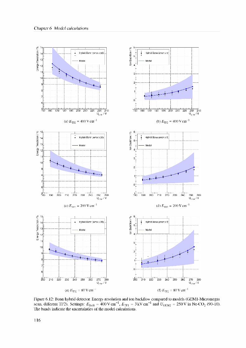
Chapter 6 Model calculations
(a) ETF2 = 100 Vcm (b) ETF2 = 100 Vcm
(c) ETF2 = 200 Vcm (d) ETF2 = 200 Vcm
(e) ETF2 = 80 V cm 1Figure 6.12: Bonn hybrid detector. Energy resolution and ion backflow compared to models (GEMl-Micromegas scan, different TF2). Settings: EDrift = 400Vcm"1, ETF1 = 3kVcm-1 and ^GEM2 = 250 V in Ne-CO2 (90-10). The bands indicate the uncertainties of the model calculations.
(f) ETF2 = 80 V cm
116
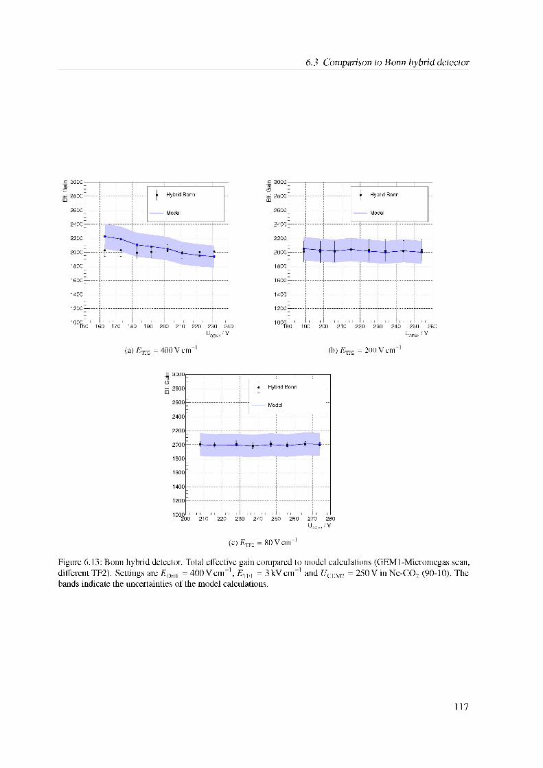
6.3 Comparison to Bonn hybrid detector
3000
2600
2400
2200
2000
1800
1600
1400
1200
02800
100050 160 170 180 190 200 210 220 230 240
UGEM1 /V
(a) ETF2 = 400 V cm (b) ETF2 = 200 V cm
(c) ETF2 = 80 V cm 1
Figure 6.13: Bonn hybrid detector. Total effective gain compared to model calculations (GEMl-Micromegas scan, different TF2). Settings are EDrift = 400 V cm"1, ETF1 = 3 kV cm"1 and GGEM2 = 250 V in Ne-CO2 (90-10). The bands indicate the uncertainties of the model calculations.
117
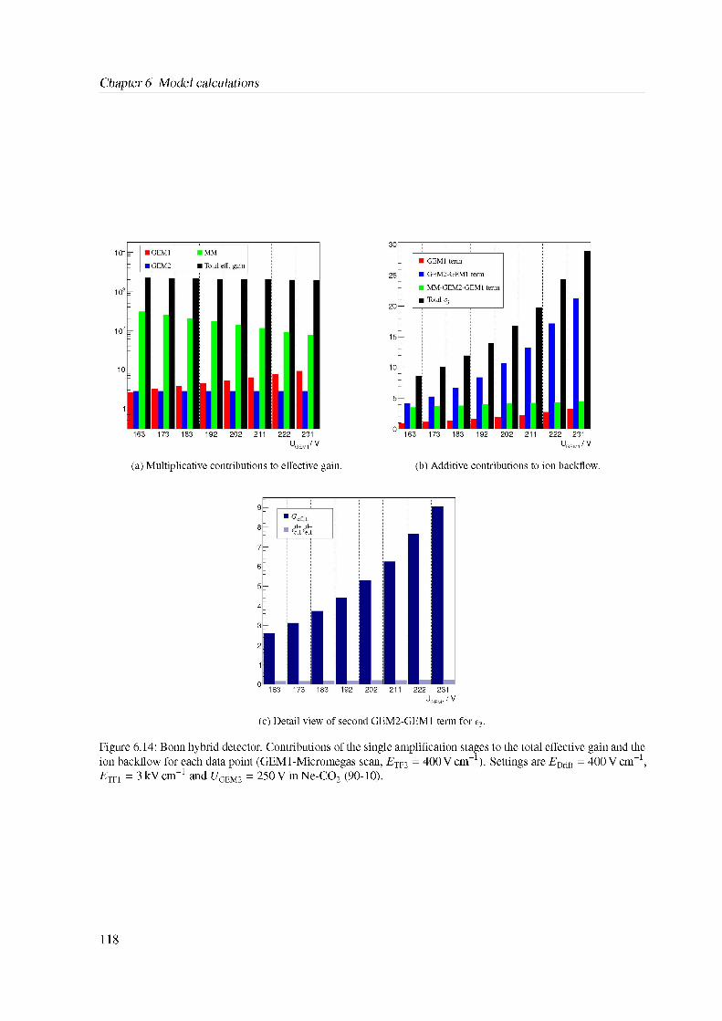
Chapter 6 Model calculations
(a) Multiplicative contributions to effective gain. (b) Additive contributions to ion backflow.
(c) Detail view of second GEM2-GEM1 term for e3.
Figure 6.14: Bonn hybrid detector. Contributions of the single amplification stages to the total effective gain and the ion backflow for each data point (GEM1-Micromegas scan, ETF2 = 400 Vcm-1). Settings are EDrift = 400 Vcm-1, ETF1 = 3kVcm-1 and ^GEM2 = 250VinNe-CO2 (90-10).
118
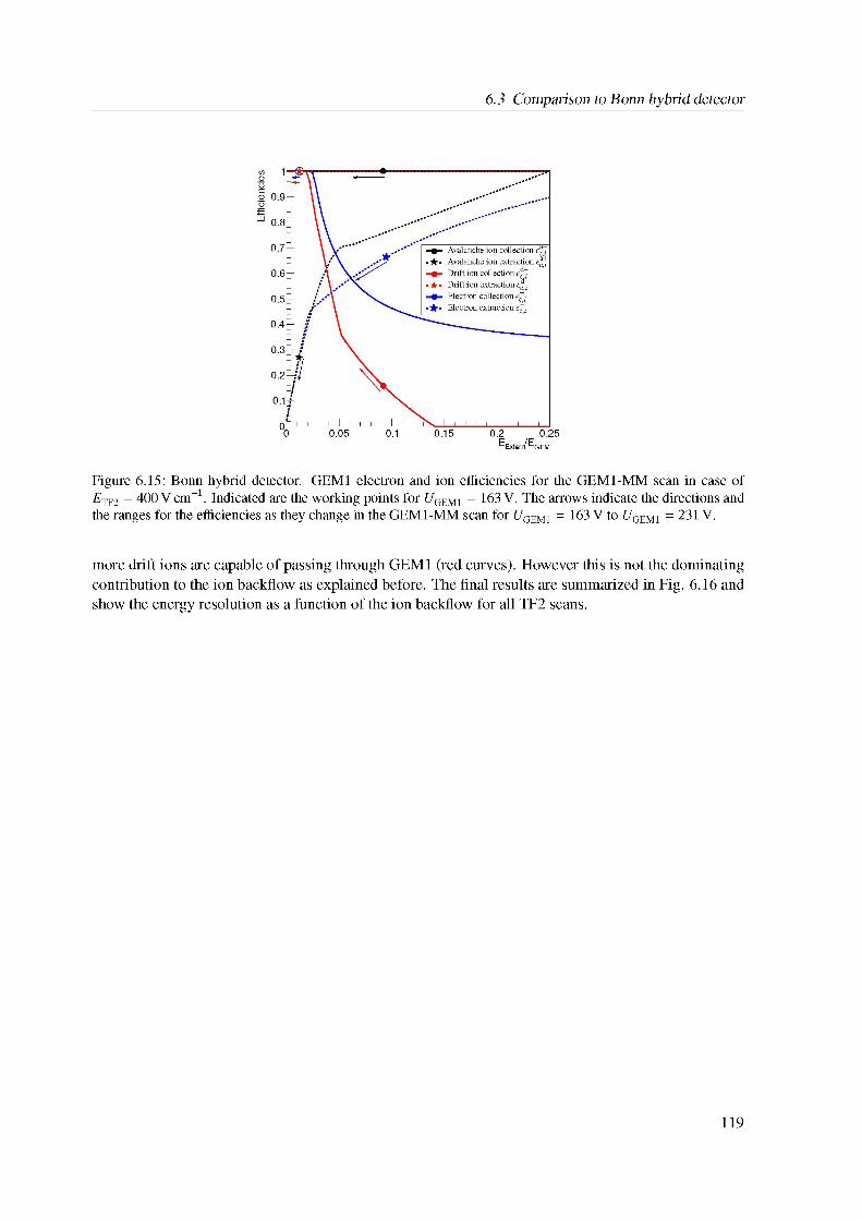
6.3 Comparison to Bonn hybrid detector
Figure 6.15: Bonn hybrid detector. GEM1 electron and ion efficiencies for the GEM1-MM scan in case of ETF2 = 400 V cm-1. Indicated are the working points for t/GEM1 = 163 V. The arrows indicate the directions and the ranges for the efficiencies as they change in the GEM1-MM scan for t/GEM1 = 163 V to t7GEM1 = 231V.
more drift ions are capable of passing through GEM1 (red curves). However this is not the dominating contribution to the ion backflow as explained before. The final results are summarized in Fig. 6.16 and show the energy resolution as a function of the ion backflow for all TF2 scans.
119
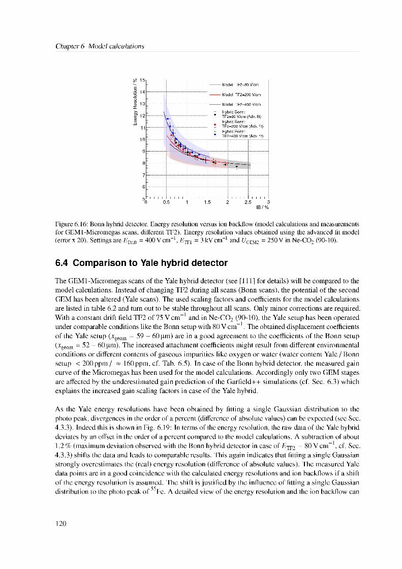
Chapter 6 Model calculations
Figure 6.16: Bonn hybrid detector. Energy resolution versus ion backflow (model calculations and measurements for GEM1-Micromegas scans, different TF2). Energy resolution values obtained using the advanced fit model (error x 20). Settings are EDrift = 400 V cm’1, ETF1 = 3kV cm’1 and 17GEM2 = 250 V in Ne-CO2 (90-10).
6.4 Comparison to Yale hybrid detector
The GEM1-Micromegas scans of the Yale hybrid detector (see [111] for details) will be compared to the model calculations. Instead of changing TF2 during all scans (Bonn scans), the potential of the second GEM has been altered (Yale scans). The used scaling factors and coefficients for the model calculations are listed in table 6.2 and turn out to be stable throughout all scans. Only minor corrections are required. With a constant drift field TF2 of 75 V cm-1 and in Ne-CO2 (90-10), the Yale setup has been operated under comparable conditions like the Bonn setup with 80 V cm-1. The obtained displacement coefficients of the Yale setup (xgeom = 59 - 60 pm) are in a good agreement to the coefficients of the Bonn setup (xgeom = 52 - 60 pm). The increased attachment coefficients might result from different environmental conditions or different contents of gaseous impurities like oxygen or water (water content Yale / Bonn setup < 200 ppm / ~ 160 ppm, cf. Tab. 6.5). In case of the Bonn hybrid detector, the measured gain curve of the Micromegas has been used for the model calculations. Accordingly only two GEM stages are affected by the underestimated gain prediction of the Garfield++ simulations (cf. Sec. 6.3) which explains the increased gain scaling factors in case of the Yale hybrid.
As the Yale energy resolutions have been obtained by fitting a single Gaussian distribution to the photo peak, divergences in the order of a percent (difference of absolute values) can be expected (see Sec.4.3.3) . Indeed this is shown in Fig. 6.19: In terms of the energy resolution, the raw data of the Yale hybrid deviates by an offset in the order of a percent compared to the model calculations. A subtraction of about1.2 % (maximum deviation observed with the Bonn hybrid detector in case of ETF2 = 80 V cm-1, cf. Sec.4.3.3) shifts the data and leads to comparable results. This again indicates that fitting a single Gaussian strongly overestimates the (real) energy resolution (difference of absolute values). The measured Yale data points are in a good coincidence with the calculated energy resolutions and ion backflows if a shift of the energy resolution is assumed. The shift is justified by the influence of fitting a single Gaussian distribution to the photo peak of 55Fe. A detailed view of the energy resolution and the ion backflow can
120
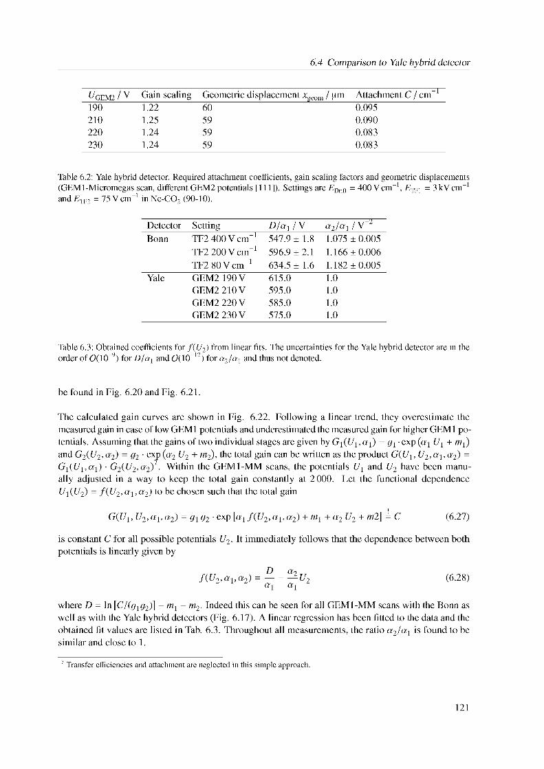
6.4 Comparison to Yale hybrid detector
Table 6.2: Yale hybrid detector. Required attachment coefficients, gain scaling factors and geometric displacements (GEMl-Micromegas scan, different GEM2 potentials [111]). Settings are EDrift = 400 Vcm"1, ETF1 = 3kV cm-1 and ETF2 = 75 Vcm-1 inNe-CO2 (90-10).
UGEM2 / V Gain scaling Geometric displacement xgeom / um Attachment C / cm 1
190 1.22 60 0.095210 1.25 59 0.090220 1.24 59 0.083230 1.24 59 0.083
Table 6.3: Obtained coefficients for f(U2) from linear fits. The uncertainties for the Yale hybrid detector are in the order of O(10“9) for D/a1 and O(10“12) for a2/a1 and thus not denoted.
Detector Setting D/a1 / V a2=a1 / V2Bonn TF2 400Vcm-1 547.9 ± 1.8 1.075 ± 0.005
TF2 200Vcm-1 596.9 ± 2.1 1.166 ± 0.006TF2 80 Vcm-1 634.5 ± 1.6 1.182 ± 0.005
Yale GEM2 190 V 615.0 1.0GEM2 210V 595.0 1.0GEM2 220 V 585.0 1.0GEM2 230 V 575.0 1.0
be found in Fig. 6.20 and Fig. 6.21.
The calculated gain curves are shown in Fig. 6.22. Following a linear trend, they overestimate the measured gain in case of low GEM1 potentials and underestimated the measured gain for higher GEM1 potentials. Assuming that the gains of two individual stages are given by G1(U1 ,a1) = g1 ■ exp (a1 U1 + m1) and G2(U2, a2) = g2 ■ exp (a2 U2 + m2), the total gain can be written as the product G(U1, U2, a1,a2) =
x7G1(U1,a1) ■ G2(U2,a2) . Within the GEM1-MM scans, the potentials U1 and U2 have been manually adjusted in a way to keep the total gain constantly at 2 000. Let the functional dependence U1(U2) = f (U2, a1,a2) to be chosen such that the total gain
G(U1; U2; a1a) = 01 02 ■ exp fU a^) + rm + a2 U2 + m2] = C (6.27)
is constant C for all possible potentials U2. It immediately follows that the dependence between both potentials is linearly given by
f(U2,a1,a2) = — - "' U2 (6.28)a1 a1
where D = ln [C/(g1g2)] - m1 - m2. Indeed this can be seen for all GEM1-MM scans with the Bonn as well as with the Yale hybrid detectors (Fig. 6.17). A linear regression has been fitted to the data and the obtained fit values are listed in Tab. 6.3. Throughout all measurements, the ratio a2/a1 is found to be similar and close to 1.
7 Transfer efficiencies and attachment are neglected in this simple approach.
121
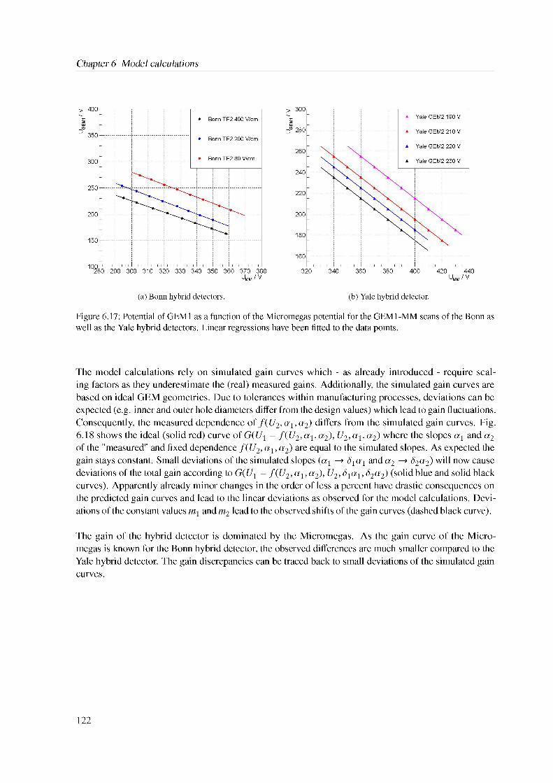
Chapter 6 Model calculations
(a) Bonn hybrid detectors.
Figure 6.17: Potential of GEM1 as a function of the Micromegas potential for the GEM1-MM scans of the Bonn as well as the Yale hybrid detectors. Linear regressions have been fitted to the data points.
(b) Yale hybrid detector.
The model calculations rely on simulated gain curves which - as already introduced - require scaling factors as they underestimate the (real) measured gains. Additionally, the simulated gain curves are based on ideal GEM geometries. Due to tolerances within manufacturing processes, deviations can be expected (e.g. inner and outer hole diameters differ from the design values) which lead to gain fluctuations. Consequently, the measured dependence of f (U2, a1,a2) differs from the simulated gain curves. Fig. 6.18 shows the ideal (solid red) curve of G(U1 = f(U2, a1, a2), U2, a1, a2) where the slopes a1 and a2
of the "measured" and fixed dependence f(U2, a1, a2) are equal to the simulated slopes. As expected the gain stays constant. Small deviations of the simulated slopes (a1 ! b1 a1 and a2 ! b2a2) will now cause deviations of the total gain according to G(U1 = f (U2, a1, a2), U2, 81a1,82a2) (solid blue and solid black curves). Apparently already minor changes in the order of less a percent have drastic consequences on the predicted gain curves and lead to the linear deviations as observed for the model calculations. Deviations of the constant values m1 and m2 lead to the observed shifts of the gain curves (dashed black curve).
The gain of the hybrid detector is dominated by the Micromegas. As the gain curve of the Micro- megas is known for the Bonn hybrid detector, the observed differences are much smaller compared to the Yale hybrid detector. The gain discrepancies can be traced back to small deviations of the simulated gain curves.
122
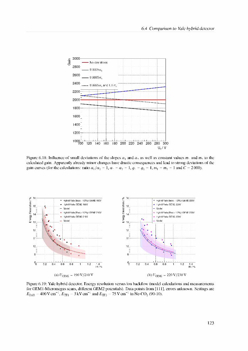
6.4 Comparison to Yale hybrid detector
Figure 6.18: Influence of small deviations of the slopes a1 and a2 as well as constant values m1 and m2 to the calculated gain. Apparently already minor changes have drastic consequences and lead to strong deviations of the gain curves (for the calculations: ratio a1/a2 = 1, a1 = a2 = 1, g1 = g2 = 1, m1 = m2 = 1 and C = 2000).
(a) Fgem2 = 190 V/210 V
Figure 6.19: Yale hybrid detector. Energy resolution versus ion backflow (model calculations and measurements for GEM1-Micromegas scans, different GEM2 potentials). Data points from [111], errors unknown. Settings are EDrift = 400 Vcm-1, ETF1 = 3kVcm-1 and ETF2 = 75Vcm-1 inNe-CO2 (90-10).
(b) Fgem2 = 220V/230V
123
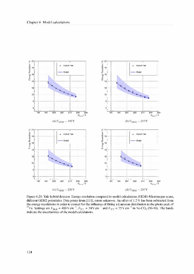
Chapter 6 Model calculations
(a) ^GEM2 = 190 V (b) UOem2 = 210 V
(c) ^Gem2 = 220 V
Figure 6.20: Yale hybrid detector. Energy resolution compared to model calculations (GEM1-Micromegas scans, different GEM2 potentials). Data points from [111], errors unknown. An offset of 1.2 % has been subtracted from the energy resolutions in order to correct for the influence of fitting a Gaussian distribution to the photo peak of 55Fe. Settings are EDrift = 400 Vcm-1, ETF1 = 3kVcm-1 and ETF2 = 75 Vcm-1 in Ne-CO2 (90-10). The bands indicate the uncertainties of the model calculations.
(d) UGem2 = 230 V
124
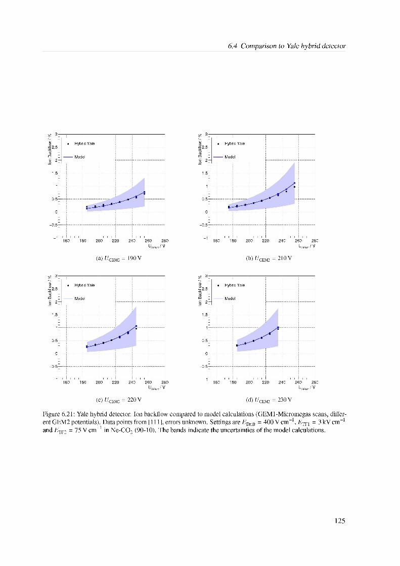
6.4 Comparison to Yale hybrid detector
(a) ^GEM2 = 190 V (b) ^GEM2 = 210 V
(c) ^GEM2 = 220 V
Figure 6.21: Yale hybrid detector. Ion backflow compared to model calculations (GEMl-Micromegas scans, different GEM2 potentials). Data points from [111], errors unknown. Settings are EDrift = 400Vcm-1, ETF1 = 3kVcm-1 and ETF2 = 75 V cm-1 in Ne-CO2 (90-10). The bands indicate the uncertainties of the model calculations.
(d) ^GEM2 = 230 V
125
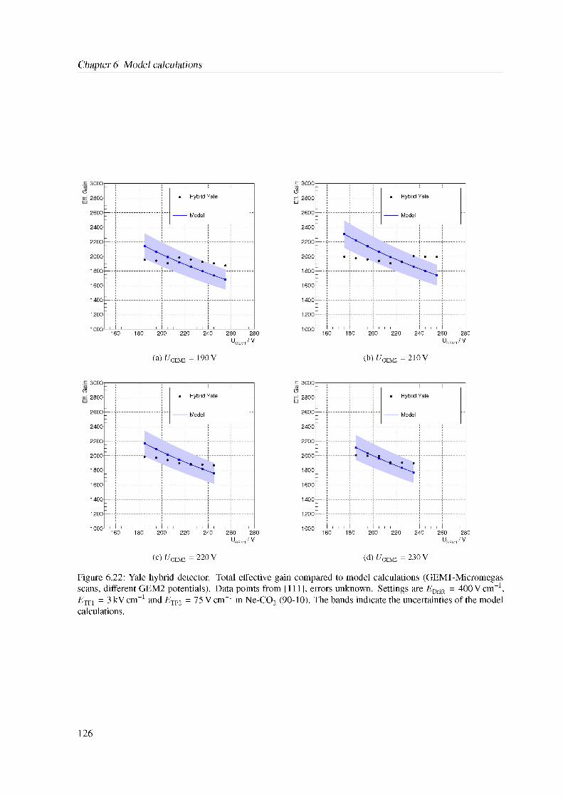
Chapter 6 Model calculations
3000
2600
2400
2200
2000
1800
1600
1400
1200
1000
02800
(a) ^GEM2 = 190 V (b) ^GEM2 = 210 V
3000
2600
2400
2200
2000
1800
1600
1400
1200
1000
02800
(c) ^GEM2 = 220 V
Figure 6.22: Yale hybrid detector. Total effective gain compared to model calculations (GEMl-Micromegas scans, different GEM2 potentials). Data points from [111], errors unknown. Settings are EDrift = 400 Vcm-1, ETF1 = 3 kV cm-1 and ETF2 = 75 V cm-1 in Ne-CO2 (90-10). The bands indicate the uncertainties of the model calculations.
(d) ^GEM2 = 230 V
126
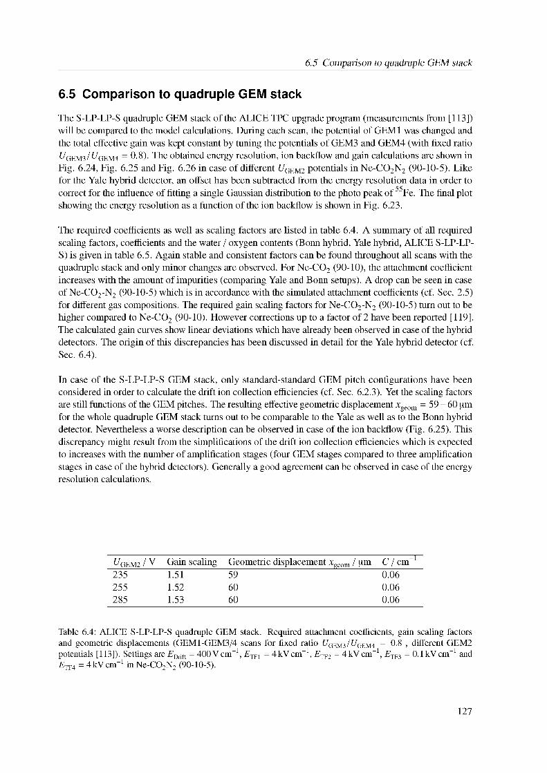
6.5 Comparison to quadruple GEM stack
6.5 Comparison to quadruple GEM stack
The S-LP-LP-S quadruple GEM stack of the ALICE TPC upgrade program (measurements from [113]) will be compared to the model calculations. During each scan, the potential of GEM1 was changed and the total effective gain was kept constant by tuning the potentials of GEM3 and GEM4 (with fixed ratio CGEM3/GGEM4 = 0-8). The obtained energy resolution, ion backflow and gain calculations are shown in Fig. 6.24, Fig. 6.25 and Fig. 6.26 in case of different CGEM2 potentials in Ne-CO2N2 (90-10-5). Like for the Yale hybrid detector, an offset has been subtracted from the energy resolution data in order to correct for the influence of fitting a single Gaussian distribution to the photo peak of 55Fe. The final plot showing the energy resolution as a function of the ion backflow is shown in Fig. 6.23.
The required coefficients as well as scaling factors are listed in table 6.4. A summary of all required scaling factors, coefficients and the water / oxygen contents (Bonn hybrid, Yale hybrid, ALICE S-LP-LP- S) is given in table 6.5. Again stable and consistent factors can be found throughout all scans with the quadruple stack and only minor changes are observed. For Ne-CO2 (90-10), the attachment coefficient increases with the amount of impurities (comparing Yale and Bonn setups). A drop can be seen in case of Ne-CO2-N2 (90-10-5) which is in accordance with the simulated attachment coefficients (cf. Sec. 2.5) for different gas compositions. The required gain scaling factors for Ne-CO2-N2 (90-10-5) turn out to be higher compared to Ne-CO2 (90-10). However corrections up to a factor of 2 have been reported [119]. The calculated gain curves show linear deviations which have already been observed in case of the hybrid detectors. The origin of this discrepancies has been discussed in detail for the Yale hybrid detector (cf. Sec. 6.4).
In case of the S-LP-LP-S GEM stack, only standard-standard GEM pitch configurations have been considered in order to calculate the drift ion collection efficiencies (cf. Sec. 6.2.3). Yet the scaling factors are still functions of the GEM pitches. The resulting effective geometric displacement xgeom = 59 - 60 pm for the whole quadruple GEM stack turns out to be comparable to the Yale as well as to the Bonn hybrid detector. Nevertheless a worse description can be observed in case of the ion backflow (Fig. 6.25). This discrepancy might result from the simplifications of the drift ion collection efficiencies which is expected to increases with the number of amplification stages (four GEM stages compared to three amplification stages in case of the hybrid detectors). Generally a good agreement can be observed in case of the energy resolution calculations.
Table 6.4: ALICE S-LP-LP-S quadruple GEM stack. Required attachment coefficients, gain scaling factors and geometric displacements (GEM1-GEM3/4 scans for fixed ratio GGEM3/CGEM4 = 0.8 , different GEM2 potentials [113]). Settings are EDrift = 400Vcm-1, ETF1 = 4kVcm-1, ETF2 = 4kVcm-1, ETF3 = 0.1kVcm-1 and ETF4 = 4kVcm“1 in Ne-CO2N2 (90-10-5).
^GEM2 /V Gain scaling Geometric displacement xgeom / pm C / cm 1
235 1.51 59 0.06255 1.52 60 0.06285 1.53 60 0.06
127
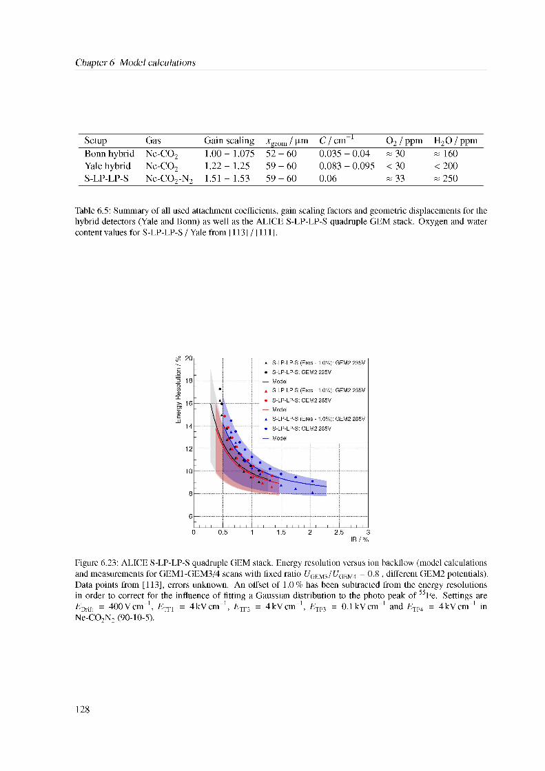
Chapter 6 Model calculations
Table 6.5: Summary of all used attachment coefficients, gain scaling factors and geometric displacements for the hybrid detectors (Yale and Bonn) as well as the ALICE S-LP-LP-S quadruple GEM stack. Oxygen and water content values for S-LP-LP-S / Yale from [113] / [111].
Setup Gas Gain scaling •^geom / bm C / cm 1 O2 /ppm H2O / ppmBonn hybrid Ne-CO2 1.00 - 1.075 52 - 60 0.035 - 0.04 « 30 « 160Yale hybrid Ne-CO2 1.22 - 1.25 59 - 60 0.083 - 0.095 < 30 < 200S-LP-LP-S Ne-CO2-N2 1.51 - 1.53 59 - 60 0.06 « 33 « 250
Figure 6.23: ALICE S-LP-LP-S quadruple GEM stack. Energy resolution versus ion backflow (model calculations and measurements for GEM1-GEM3/4 scans with fixed ratio I7geM3/^geM4 = 0-8 , different GEM2 potentials). Data points from [113], errors unknown. An offset of 1.0 % has been subtracted from the energy resolutions in order to correct for the influence of fitting a Gaussian distribution to the photo peak of 55Fe. Settings are EDrift = 400Vcm-1, ETF1 = 4kVcm-1, ETF2 = 4kVcm-1, ETF3 = 0.1kVcm-1 and ETF4 = 4kVcm-1 in Ne-CO2N2 (90-10-5).
128
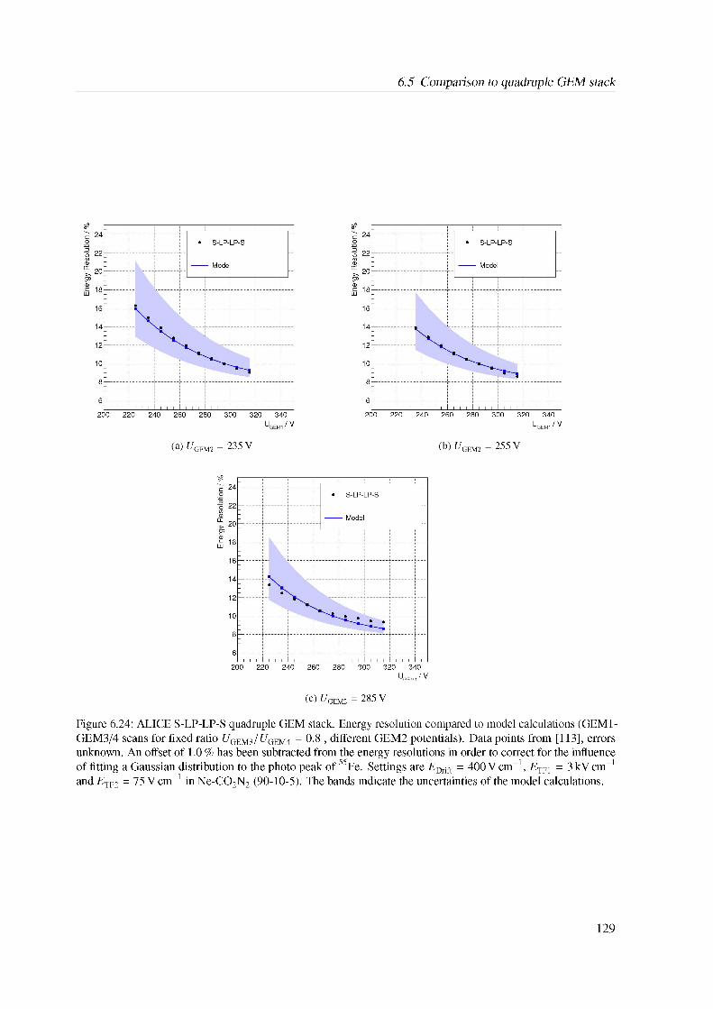
6.5 Comparison to quadruple GEM stack
(a) ^GEM2 = 235 V (b) ^Gem2 = 255 V
UGEM1/V
(c) UGEM2 = 285 V
Figure 6.24: ALICE S-LP-LP-S quadruple GEM stack. Energy resolution compared to model calculations (GEM1- GEM3/4 scans for fixed ratio UGEM3/ UGEM4 = 0.8 , different GEM2 potentials). Data points from [113], errors unknown. An offset of 1.0 % has been subtracted from the energy resolutions in order to correct for the influence of fitting a Gaussian distribution to the photo peak of 55Fe. Settings are EDrift = 400 V cm-1, ETF1 = 3 kV cm-1 and ETF2 = 75 V cm-1 in Ne-CO2N2 (90-10-5). The bands indicate the uncertainties of the model calculations.
129
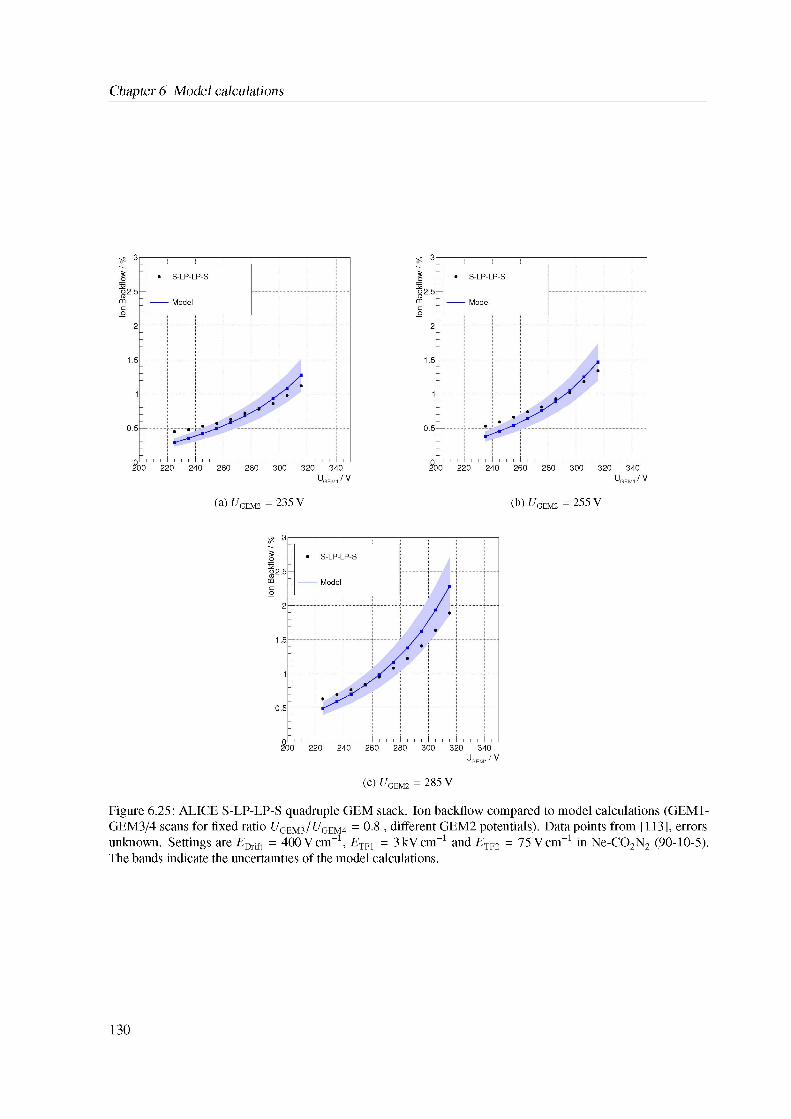
Chapter 6 Model calculations
(a) ^gem2 = 235 V (b) ^gem2 = 255 V
(c) ^Gem2 = 285 V
Figure 6.25: ALICE S-LP-LP-S quadruple GEM stack. Ion backflow compared to model calculations (GEM1- GEM3/4 scans for fixed ratio CGEM3/ CGEM4 = 0.8 , different GEM2 potentials). Data points from [113], errors unknown. Settings are EDrift = 400Vcm-1, ETF1 = 3kVcm-1 and ETF2 = 75Vcm-1 in Ne-CO2N2 (90-10-5). The bands indicate the uncertainties of the model calculations.
130
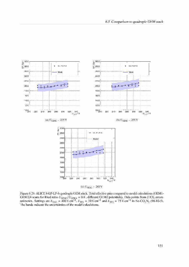
6.5 Comparison to quadruple GEM stack
(a) ^gem2 = 235 V (b) ^gem2 = 255 V
(c) ^Gem2 = 285 V
Figure 6.26: ALICE S-LP-LP-S quadruple GEM stack. Total effective gain compared to model calculations (GEM1- GEM3/4 scans for fixed ratio CGEM3/ CGEM4 = 0.8 , different GEM2 potentials). Data points from [113], errors unknown. Settings are EDrift = 400Vcm-1, ETF1 = 3kVcm-1 and ETF2 = 75Vcm-1 in Ne-CO2N2 (90-10-5). The bands indicate the uncertainties of the model calculations.
131
Chapter 6 Model calculations
6.6 Implementation in the ALICE O framework2
8 https://github.com/AliceO2Group/AliceO2
Due to the upgrade of ALICE and the increased data rates during the continuous readout, a new computational concept is currently in development which will be used for the online as well as for the offline (Online - Offline, O2) data reconstruction and analysis during Run 3 and Run 4 of the LHC. A major aspect of the upgrade is the immediate transfer of all detector data to the O2 computing farm. The O2 system performs detector calibration and data reconstruction online, e.g. cluster finders reduce the amount of data on-the-fly by replacing the raw data. Only reconstructed data will be processed and stored permanently. Raw data will be discarded. Up to now the reconstruction was done fully offline. Detailed information about the upgrade concept of the ALICE O2 computing system can be found in the dedicated Technical Design Report [120]. The ALICE O2 software repository8 is developed from scratch and uses state of the art C++ and modern coding concepts. It includes the relevant and detector specific source code for the reconstruction, the calibration and the simulation of the ALICE experiment.
The models of the electron charge transfers and the energy resolutions have been added to the TPC implementation and allow to dynamically calculate the efficiencies as a function of the electrostatic field configuration and the applied GEM potentials. Prior to this these values have been hard-corded. The gains of the individual stages as well as the energy resolution of the stack can now be immediately calculated. The implemented energy resolution curves are adjusted on the outcome of the comparison of the S-LP-LP-S stack to the model calculations (cf. Sec. 6.5). The implementation in O2 is based on a simplified version of the C++ class presented in Sec. 6.3. An example source code which allows to reproduce the energy resolution and the gain of the ALICE baseline configuration (cf. Sec. 6.5) with the ALICE O2 framework is given in the appendix A.2.
132
CHAPTER 7
Summary
In the context of the ongoing upgrade of the Large Hadron Collider at CERN, the interaction rate of ALICE will be increased to 50 kHz for Pb-Pb collisions. As a consequence, a continuous readout of the Time Projection Chamber will be required which was previously limited to rates in the order of 300 Hz due to a gated readout system based on Multiwire Proportional Chambers. To keep the amount of space-charge distortions at a manageable size, the ion backflow of the charge amplification system has to be significantly reduced. At the same time an excellent detector performance and stability of the system has to be maintained. In Ne-CO2-N2 (90-10-5) and at a total gain of 2 000, the energy resolution must not exceed 12 % for 55Fe which translates to a dE/dx resolution of about 5.5 % and 7 % in pp and central Pb-Pb collisions. The ion backflow should be lower than 1 % in order to be able to completely correct all effects from space-charge distortions. A solution with four GEM foils (S-LP-LP-S configuration) has been adopted as baseline solution for the upgraded chambers, as the concept of GEM detector was more studied and understood at the time of the decision.
7.1 Experimental setup
As an alternative approach to the ALICE baseline solution for the upgrade of the Time Projection Chamber, a hybrid GEM-Micromegas detector consisting of one Micromegas and two GEM foils has been assembled and investigated in terms of the energy resolution, the ion backflow and the gain. Micromegas offer an intrinsic suppression of the ion backflow in the order of a few percent at relatively high gains. As a consequence less GEM stages are required to block the back drifting ions. The GEM foils are commonly used as preamplification stages in order to reduce the needed gain of the Micromegas and to keep the discharge probability at a reasonable level.
The investigated setup consisted of two standard-pitch GEM foils (pitch of 140 pm) with an active area of 10 cm x 10 cm. A bulk Micromegas with a gap of 128 pm and a mesh with approximately 160 lines / cm has been operated as last stage. The whole setup has been assembled within a gas-tight vessel with a volume of about 6 liters. Premixed gas bottles were used in order to flush the setup with Ne-CO2 (90-10) and flows of about 2 - 6 L h-1. A Kapton window on the lid and on the side of the vessel allowed to externally irradiate the drift volume with an 55Fe source and an X-ray tube (Mini-X from Amptek). The pressure, the water as well as the oxygen content was monitored using a Rapidox device.
A summation card has been designed in order to sum up the 128 pads at the segmented readout plane. The card can be directly connected to the Micromegas and is placed inside the vessel. Different configurations
133
Chapter 7 Summary
can be selected, allowing to read out only the innermost pads up to the full pad plane.
Within the scope of this work, a slow control has been developed in LabView which gives full access to control and to operate Micro-Pattern Gaseous Detectors (MPGD) such as GEM stacks or the hybrid detector. The operation can be fully automated by user-defined script files which can be loaded and executed within the slow control. This allows to run dedicated measurements over long time scales, e.g. ramp to specific voltage settings, start or stop current measurements, record and save MCA spectra and more. The slow control is capable of communicating with the Bonn pA-meters as well as with the Zagreb pA-meters which are used within the QA program of the ALICE TPC upgrade. The slow control has become the new standard for MPGD operation in the laboratories.
7.2 Background I Energy resolution studies
A common way to determine the energy resolution (in terms of a/p) is to fit a single Gaussian distribution to the photo peak of 55Fe spectra. In fact, the photo peak consists of two energy lines (Ka and Kp) which is neglected in this case as they can not be resolved with the achievable energy resolution given by gaseous detectors. The influence of the suppressed Kp line was studied by looking at the possible Gamma and Auger electron emissions. Comparing both methods indicates that fitting a single Gaussian distribution overestimates the energy resolutions, i.e. the Kp peak should be taken into account. Additionally a small excitation of copper was studied as copper layers are irradiated as well (like copper layers of the GEM foils or the cathode): Copper excitations are expected with a probability of a few percent and lead to minor changes of the energy resolutions, i.e. the influence of copper excitations can be neglected.
A dedicated study of the recorded MCA spectra for three different conditions of irradiation (55Fe collimated / not collimated from top window, collimated from side window) indicates that the background is composed of two different contributions: Sharing causes (with approximately 68 % of background contribution) a lower energetic tail on the left side of the photo peak and appears if charges from photo conversions are partially lost. This effects dominates in case of uncollimated or displaced sources (with respect to the readout pads) as more photons convert in the vicinity of the investigated pads. The second background contribution (approximately 32 %) appears as an intrinsic broad exponential component of the detector and an estimation of the background rate yields that cosmics can be excluded. Both background contributions are correlated by different conditions of irradiation, i.e. a subtraction of two recorded background spectra (under different conditions) results in the third background spectrum.
Based on the background studies and the investigations of the Kp line, a fit model has been derived in order to describe the full MCA spectra. This model takes sharing (modeled by the product of an error function and a linear function) as well as the second broad exponential background contribution into account. Both the Ka as well as the Kp lines are described by Gaussian functions which are coupled by their ratios of intensities and amplitudes. A further exponential function is used in order to describe the lower energetic electronic noise given by the readout electronics. Comparing the advanced fit model to the method of fitting a single Gaussian distribution to the tip of the photo peak yields that the energy resolutions differ in a range between 1 - 2 % (difference of absolute values, energy resolutions obtained by a single Gaussian function are overestimated). Consequently a proper description of the background and the inclusion of the Kp line should be always considered.
134
7.3 Measurements and comparison to Yale hybrid/ quadruple GEM stack
7.3 Measurements and comparison to Yale hybrid I quadruple GEM stack
The hybrid detector has been investigated within GEMl-Micromegas scans in Ne-CO2 (90-10) and for different transfer fields between the second GEM and the Micromegas. The potential of the first GEM stage has been scanned while adjusting the Micromegas potential in order to achieve a constant gain of 2 000. The measurements of the ion backflow and the energy resolution clearly show that the hybrid detector fulfills the requirements of the ALICE TPC upgrade (energy resolution a/p < 12 % for 55Fe and ion backflow < 1 % at a gain of 2000). By using the advanced fit model for the energy resolution, a value of about a/p - 10 % and an ion backflow of 0.7 % can be achieved. To allow for a comparison with the ALICE S-LP-LP-S baseline solution, a single Gaussian distribution has been fitted to the photo peak as well. In this case the hybrid detector clearly competes with the quadruple GEM stack in terms of ion backflow and energy resolution. A comparison to an alternative hybrid setup of the Yale University allows to reproduce a specific GEM1-Micromegas scan. A crosscheck of some specific settings allows to reproduce the gain as well as the ion backflow. However divergences of about 0.5 - 1.0 % (difference of absolute values) can be observed for the energy resolution. Nevertheless both detectors lead to comparable measurements and do not indicate major inconsistent behaviors. Within the limits of the given measurable accuracy and the environmental uncertainties, trends of the detector performances can be reproduced.
7.4 Model calculations
Characteristic quantities of MPGD (like energy resolution, ion backflow and gain) highly depend on the charge transfer processes between the individual amplification stages. The charge transfer between multiple GEM stages can be described by the collection as well as the extraction efficiencies. The collection efficiency describes the probability to collect the charge carriers into the holes of the GEM foil. Accordingly the extraction efficiency describes the probability of extraction the charges to the next amplification stage or the readout plane. Within this work, an analytic model has been derived in order to describe the transfer efficiencies for an arbitrary GEM geometry and electrostatic configuration. The model is based on a two-dimensional and simplified cut of the hexagonal GEM structure. The GEM electrodes as well as the anode and the cathode are modeled by constant charge distributions. No polyimide layer is considered. The geometry of the GEM is defined in terms of the pitch, the thickness and the hole diameter (no differentiation between an inner and an outer diameter). Based on the charge distribution, the electric field can be obtained by solving Poisson’s equation.
The electric field calculations inside a GEM hole show that the average electric field can be expressed as the field of a parallel plate capacitor where an additional deviation factor is required. The deviation factor k can be expressed in terms of the GEM geometry and lower orders are derived. Three-dimensional calculations for a standard-pitch GEM lead to a value of k3D = 0.7408 which is in a good agreement to observed measurements (0.73 to 0.825 [118]). The average field above or below a GEM (e.g. induction field, transfer field) can be well approximated as the field of a parallel plate capacitor. In this case the deviation factor can be neglected.
Electric flux calculations lead to closed analytic expressions of the efficiencies as functions of the charge density ratios. The obtained equations inherently include the appropriate limits and offsets that can be seen in simulations so far. Both the collection as well as the extraction efficiency turn out to be
135
Chapter 7 Summary
correlated by common geometric coefficients. In addition correlations between the coefficients can be derived. Most coefficients already show a sufficient convergence in case of lower number of GEM holes for N > 100. Analytic limits are derived in case of N ! m which allow to express the limitations and offsets of the efficiencies in terms of the optical transparency and the geometry of the GEM. Generally three characteristic regions of the efficiency curves can be observed which can be traced back to three different electric field line scenarios.
As the obtained efficiencies are solely based on two-dimensional electric field calculations, a certain deviation to simulations can be expected as no polyimide layers and no gas properties such as diffusion have been taken into account. Furthermore this model is based on the assumption of constant charge density distributions. Numerical calculations of three-dimensional GEM structures in ANSYS allow to obtain the charge distributions on the electrodes if constant potentials and electric fields are assumed. The assumption of a constant charge density distribution on the anode and the cathode turns out to be applicable for distances exceeding 1000 pm which is usually the case. However non-constant distributions can be observed on the GEM electrodes. In fact, this turns out to be a strong simplification of the model calculations. By introducing three tuning parameters, an appropriate transformation of the geometric parameters becomes possible, allowing to correct for the electrostatic simplifications and to include diffusion. Both tuning factors to correct for the electrostatic simplifications scale with the pitch of the GEM. The diffusion factor turns out to be independent of the pitch and changes with the gas composition. Finally the efficiencies can be calculated for an arbitrary electric field configuration and GEM pitch.
The derived transfer efficiencies can be used in combination with the gains of the amplification stages to calculate the effective gain of GEM stacks. A model has been introduced to calculate the energy resolution a/p in which each GEM stage contributes with the corresponding single gain fluctuation and the number of collected electrons. Furthermore, a closed analytic expression has been found for the ion backflow as a function of the individual gains and electron as well as ion transfer efficiencies. The number of back drifting ions per incoming electron e can be traced back to the charge transfers and gains of the individual stages. An important aspect is the differentiation between drift and avalanche ion efficiencies: Avalanche ions (i.e. ions created within an avalanche processes inside of a GEM hole) show different transfer properties as drift ions which enter the GEM (i.e. ions which emerged from previous amplification processes / GEMs). Drift (avalanche) ions are almost completely extracted (collected). The drift ion collection as well as the avalanche ion extraction scale with the according external electric fields. An important aspect is the initial distribution of the ions which enter a GEM as drift ions. These distributions highly influence the drift ion collection efficiency. Within the two-dimensional charge transfers calculations, two GEM foils of equal pitches have been placed on top of each other, allowing to calculate the drift ion collection efficiencies. Depending on the displacement of both GEM foils and the electrostatic configuration, strong suppressions of the drift ion collection efficiencies can be observed; Mostly dominated by the geometric blocking of two GEM foils.
The derived model calculations give access to a flexible, time-saving and in-depth study of the internal processes and dynamics of GEM stacks. In this context a C++ class has been developed which allows to define GEM stacks in terms of the geometry (e.g. GEM types, distances) and the electrostatic configuration (e.g. GEM potentials, transfer fields). The energy resolution, the ion backflow as well as the gain can be immediately calculated. The contributions of the individual GEM stages to the stack properties can be studied in detail and the working points (at which ion or electron efficiencies do the single GEM stages operate) can be indicated.
136
1.4 Model calculations
The GEMl-Micromegas scans of the Bonn and the Yale hybrid detectors show a good agreement to the model calculations in terms of the ion backflow and the energy resolution. In case of the Yale setup, a constant offset has been subtracted for the energy resolution. The offset is justified by comparing both methods (advanced fit model versus simple Gaussian distribution) to determine the energy resolution in case of the Bonn hybrid detector. Gain scaling factors are still required as the simulated gain curves are known to underestimate the (real) measured gains. The obtained scaling factors are consistent within each measurement and between both detector setups. The calculated gains show a linear trend which can not be observed in the data. This discrepancies can be traced back to small deviations between the simulated gain curves and the measured voltage dependencies within the GEMl-Micromegas scans. Indeed already minor deviations of the slopes (less than a percent) can lead to the observed deviations. The discrepancies are stronger in case of the Yale hybrid detector, since the dominating gain curve of the Micromegas is known in case of the Bonn setup. The geometric displacement between both standard-pitch GEM foils turns out to be consistent within the measurements and between both detector setups. With approximately 50 - 60 pm, the displacement is comparable to three-dimensional calculations of the hexagonal structure for large-sized GEM foils [42]. The energy resolutions of the ALICE S-LP-LP-S configuration can be well described by the model calculations. As the drift ion collection efficiencies are only calculated for standard-standard GEM pitch configurations (tuning factors are still functions of the GEM types), smaller discrepancies can be found in case of the ion backflow. Like for the hybrid detectors, linear deviations can be observed for the gain curves.
The model calculations of the electron efficiencies, the energy resolution and the gain have been implemented in the ALICE O2 framework which will be used by ALICE at CERN for Run 3 and Run 4. The implementations allow to calculate immediately these properties as functions of the electrostatic configuration (electric fields, GEM potentials) as well as the geometric setup (GEM types, distances).
137

CHAPTER 8
Outlook
The hybrid detector has been investigated in terms of the energy resolution, the ion backflow as well as the gain and competes with the S-LP-LP-S baseline solution for the upgrade of the ALICE Time Projection Chamber. A further important aspect is the discharge probability and the rate stability. Although studies of a 2GEM+MM setup at the Super Proton Synchrotron (SPS) and the Proton Synchrotron (PS) at CERN yield a reduced discharge stability compared to the quadruple GEM stack, an experimental investigation has not been carried out in case of the Bonn hybrid detector.
The origin of the broad exponential background component as it can be seen in the recorded MCA spectra is not known yet. Copper excitations and cosmics can be excluded. The background might be caused by intrinsic electronic noise of the hybrid detector itself as it disappears once the setup has been disconnected from the readout chain and the data acquisition.
The constant charge density distribution of the GEM electrodes is a strong assumption of the twodimensional efficiency calculations. ANSYS calculations showed that the charges accumulate at the rims of the GEM holes. Instead of assuming a single step function to describe the electrodes between the GEM holes, multiple step functions with different charge amplitudes can be considered. The ratios of the amplitudes are thereupon modeled according to the outcome of the ANSYS simulations. Within iterating steps, a more realistic charge density distribution of higher orders might be approached which approximates the real charge distribution. A further promising ansatz to describe the charge distribution in a continuous way is given in [121] where the surface charge has been derived in case of a conducting circular disk with a fixed electric potential. The introduced radial behavior of the charge distribution a(r) / (r2 - r2^ (where R is the radius of the disc, i.e. the diameter corresponds to the distance (w - L)=2 between two GEM holes in the model calculations) shows the observed charge accumulations of the ANSYS calculations and leads to constant potentials on the disc electrodes.
The ion-backflow model relies strongly on the simulated ion efficiencies. Two-dimensional calculations of the drift ion collection efficiencies (for two GEMs with equal pitches) already indicate that a proper and full description turns out to be complex which is still an open issue. Dedicated studies and particularly simulations are still needed in order to fully understand the drift ion efficiencies and to extend the model calculation class with more realistic efficiency curves.
The calculated values of the energy-resolution model are strongly biased by the curves of the single gain fluctuations. Up to now an empirical function has been implemented which is motivated by the
139
Chapter8 Outlook
outcome of simulations. However a more detailed investigation of the single gain fluctuations might lead to more optimized functional expressions. Additionally scalings of the gains are still required as the simulations underestimate the real gains. This issue is already known for Garfield++, yet not understood. Up to now only a constant attachment factor is globally assumed for the whole GEM stack which is manually specified. In fact, the attachment factor depends on the gas, the amount of impurities (water and oxygen content) and the applied electric field. An advanced implementation of the attachment requires a detailed simulation of the whole parameter space in order to obtain suitable lookup tables. Alternatively, an instance of Garfield++ could be included in the C++ class of the model calculations, allowing to calculate the attachment factors on-the-fly.
Up to now only the gain as well as the energy-resolution model have been implemented in the O2 framework of the ALICE experiment. As the treatment of the drift ion efficiencies is still an open issue, no ion-backflow model has been implemented yet. The energy-resolution model allows to calculate a/p for the 55Fe photo peak. A translation back to the dE/dx energy resolution for Pb-Pb and pp collisions is still an open issue.
Although still adjustments are required for the models (e.g. gain scaling, GEM displacement or attachment), the calculations open the door to a huge field of detailed investigations of MPGD and trends / relative changes can be reproduced. The influence of each stage can be quickly studied. The efficiencies and the contributions of the single stages to the whole detector can be examined. How is the gain composited? How and at which stages do the electrons or ions contribute to the ion backflow or the energy resolution? The model calculations offer great opportunities for in-depth studies of the processes within multiple amplification stages, making the dynamics inside of Micropattern Gaseous Detectors much more accessible and transparent.
140
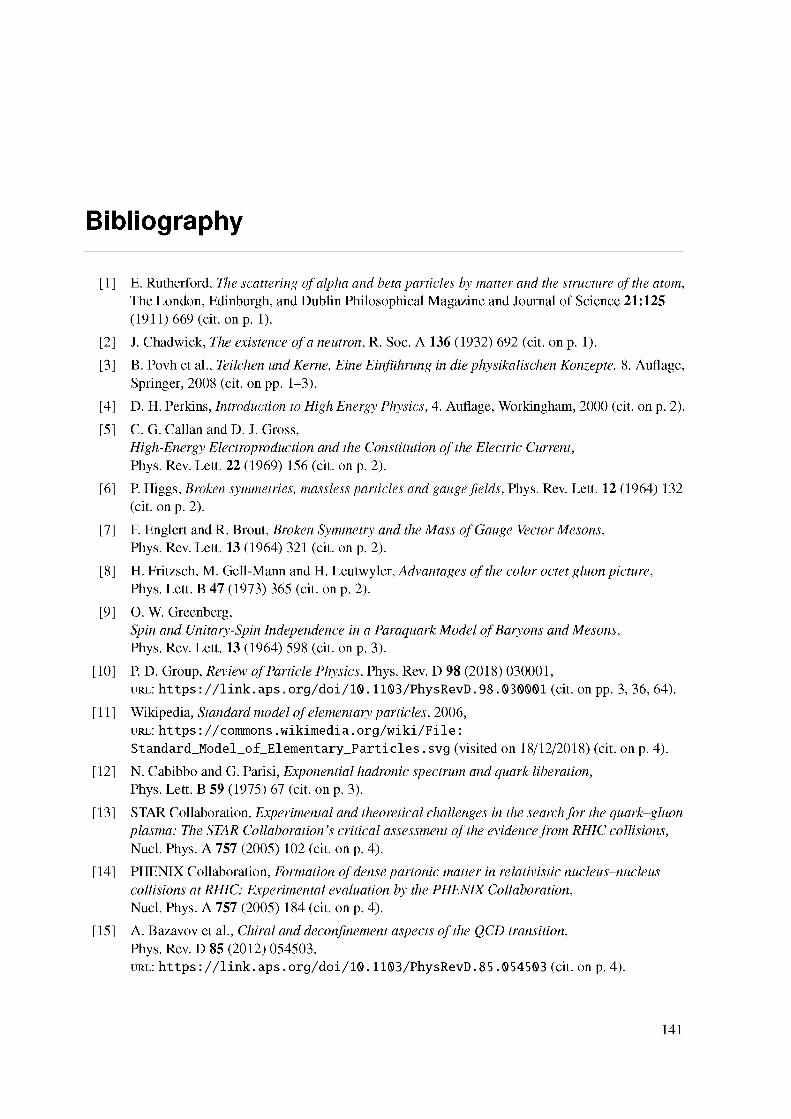
Bibliography
[1] E. Rutherford, The scattering of alpha and beta particles by matter and the structure of the atom,
(cit. onp. .The London, Edinburgh, and Dublin Philosophical Magazine and Journal of Science 21:125(1911) 669 1)
[2] J. Chadwick, The existence of a neutron, (cit. on p. . R. Soc. A 136 (1932) 692 1)
[3] B. Povh et al., Teilchen und Kerne, Eine Einfuhrung in die physikalischen Konzepte. 8. Auflage, Springer, 2008 (cit. on pp. . 1-3)
[4] D. H. Perkins, Introduction to High Energy Physics, 4. Auflage, Workingham, 2000 (cit. on p. . 2)
[5] C. G. Callan and D. J. Gross,High-Energy Electroproduction and the Constitution of the Electric Current, Phys. Rev. Lett. 22 (1969) 156 (cit. on p. 2).
[6] P. Higgs, Broken symmetries, massless particles and gauge fields, (cit. on p. .
Phys. Rev. Lett. 12 (1964) 132 2)
[7] F. Englert and R. Brout, Broken Symmetry and the Mass of Gauge Vector Mesons, (cit. on p. .Phys. Rev. Lett. 13 (1964) 321 2)
[8] H. Fritzsch, M. Gell-Mann and H. Leutwyler, Advantages of the color octet gluon picture, (cit. on p. .Phys. Lett. B 47 (1973) 365 2)
[9] O. W. Greenberg,Spin and Unitary-Spin Independence in a Paraquark Model of Baryons and Mesons, Phys. Rev. Lett. 13 (1964) 598 (cit. on p. 3).
[10] P. D. Group, Review of Particle Physics, Phys. Rev. D 98 (2018) 030001,url: https://link.aps.org/doi/10.1103/PhysRevD.98.030001 (cit. on pp. 3, 36, 64).
[11] Wikipedia, Standard model of elementary particles, 2006,url: https://commons.wikimedia.org/wiki/File:Standard_Model_of_Elementary_Particles.svg (visited on 18/12/2018) (cit. on p. 4).
[12] N. Cabibbo and G. Parisi, Exponential hadronic spectrum and quark liberation, (cit. on p. .Phys. Lett. B 59 (1975) 67 3)
[13] STAR Collaboration, Experimental and theoretical challenges in the search for the quark-gluon plasma: The STAR Collaboration's critical assessment of the evidence from RHIC collisions,
(cit. on p. .Nucl. Phys. A 757 (2005) 102 4)
[14] PHENIX Collaboration, Formation of dense partonic matter in relativistic nucleus-nucleus collisions at RHIC: Experimental evaluation by the PHENIX Collaboration,Nucl. Phys. A 757 (2005) 184 (cit. on p. 4).
[15] A. Bazavov et al., Chiral and deconfinement aspects of the QCD transition, Phys. Rev. D 85 (2012) 054503,url: https://link.aps.org/doi/10.1103/PhysRevD.85.054503 (cit. on p. 4).
141
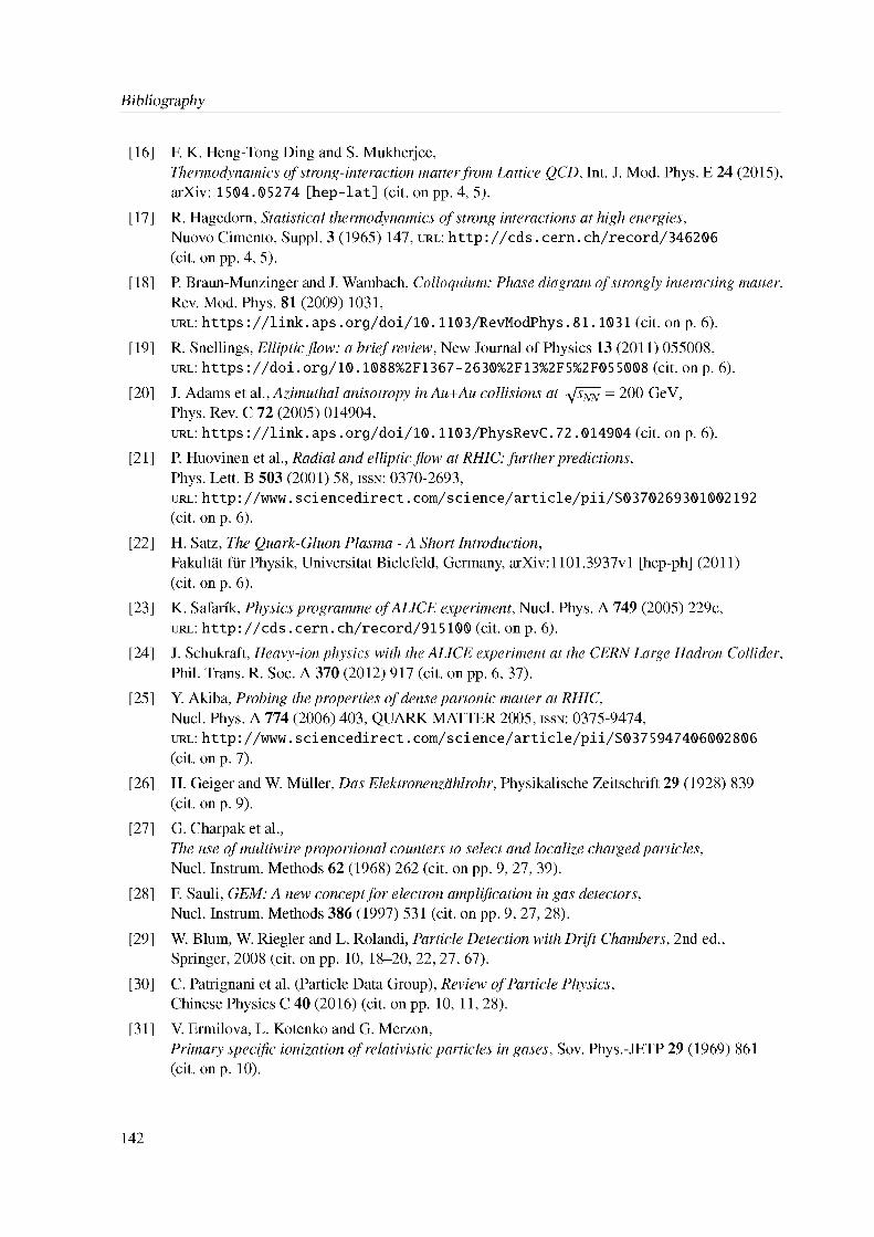
Bibliography
[16] F. K. Heng-Tong Ding and S. Mukherjee,Thermodynamics of strong-interaction matter from Lattice QCD, Int. J. Mod. Phys. E 24 (2015), arXiv: 1504.05274 [hep-lat] (cit. onpp. 4, 5).
[17] R. Hagedorn, Statistical thermodynamics of strong interactions at high energies, Nuovo Cimento, Suppl. 3 (1965) 147, url: (cit. on pp. .
http://cds.cern.ch/record/346206 4, 5)
[18] P. Braun-Munzinger and J. Wambach, Colloquium: Phase diagram of strongly interacting matter, Rev. Mod. Phys. 81 (2009) 1031,url: https://link.aps.org/doi/10.1103/RevModPhys.81.1031 (cit. on p. 6).
[19] R. Snellings, Elliptic flow: a brief review, url: (cit. onp. .
New Journal of Physics 13 (2011) 055008, https://doi.org/10.1088%2F1367-2630%2F13%2F5%2F055008 6)
[20] J. Adams et al., Azimuthal anisotropy in Au+Au collisions at psNN = 200 GeV, Phys. Rev. C 72 (2005) 014904,url: https://link.aps.org/doi/10.1103/PhysRevC.72.014904 (cit. on p. 6).
[21] P. Huovinen et al., Radial and elliptic flow at RHIC: further predictions,Phys. Lett. B 503 (2001) 58, issn: 0370-2693,url: http://www.sciencedirect.com/science/article/pii/S0370269301002192 (cit. on p. 6).
[22] H. Satz, The Quark-Gluon Plasma - A Short Introduction,Fakultat fur Physik, Universitat Bielefeld, Germany, arXiv:1101.3937v1 [hep-ph] (2011) (cit. on p. 6).
[23] K. Safarfk, Physics programme of ALICE experiment, Nucl. Phys. A 749 (2005) 229c, url: (cit. onp. . http://cds.cern.ch/record/915100 6)
[24] J. Schukraft, Heavy-ion physics with the ALICE experiment at the CERN Large Hadron Collider, Phil. Trans. R. Soc. A 370 (2012) 917 (cit. on pp. . 6, 37)
[25] Y. Akiba, Probing the properties of dense partonic matter at RHIC,Nucl. Phys. A 774 (2006) 403, QUARK MATTER 2005, issn: 0375-9474, url: http://www.sciencedirect.com/science/article/pii/S0375947406002806 (cit. on p. 7).
[26] H. Geiger and W. Muller, Das Elektronenzdhlrohr, Physikalische Zeitschrift 29 (1928) 839 (cit. on p. . 9)
[27] G. Charpak et al.,The use of multiwire proportional counters to select and localize charged particles, Nucl. Instrum. Methods 62 (1968) 262 (cit. on pp. 9, 27, 39).
[28] F. Sauli, GEM: A new concept for electron amplification in gas detectors, Nucl. Instrum. Methods 386 (1997) 531 (cit. on pp. . 9, 27, 28)
[29] W. Blum, W. Riegler and L. Rolandi, Particle Detection with Drift Chambers, 2nd ed., Springer, 2008 (cit. on pp. . 10, 18-20, 22, 27, 67)
[30] C. Patrignani et al. (Particle Data Group), Review of Particle Physics, Chinese Physics C 40 (2016) (cit. on pp. . 10, 11, 28)
[31] V. Ermilova, L. Kotenko and G. Merzon,Primary specific ionization of relativistic particles in gases, Sov. Phys.-JETP 29 (1969) 861 (cit. on p. 10).
142
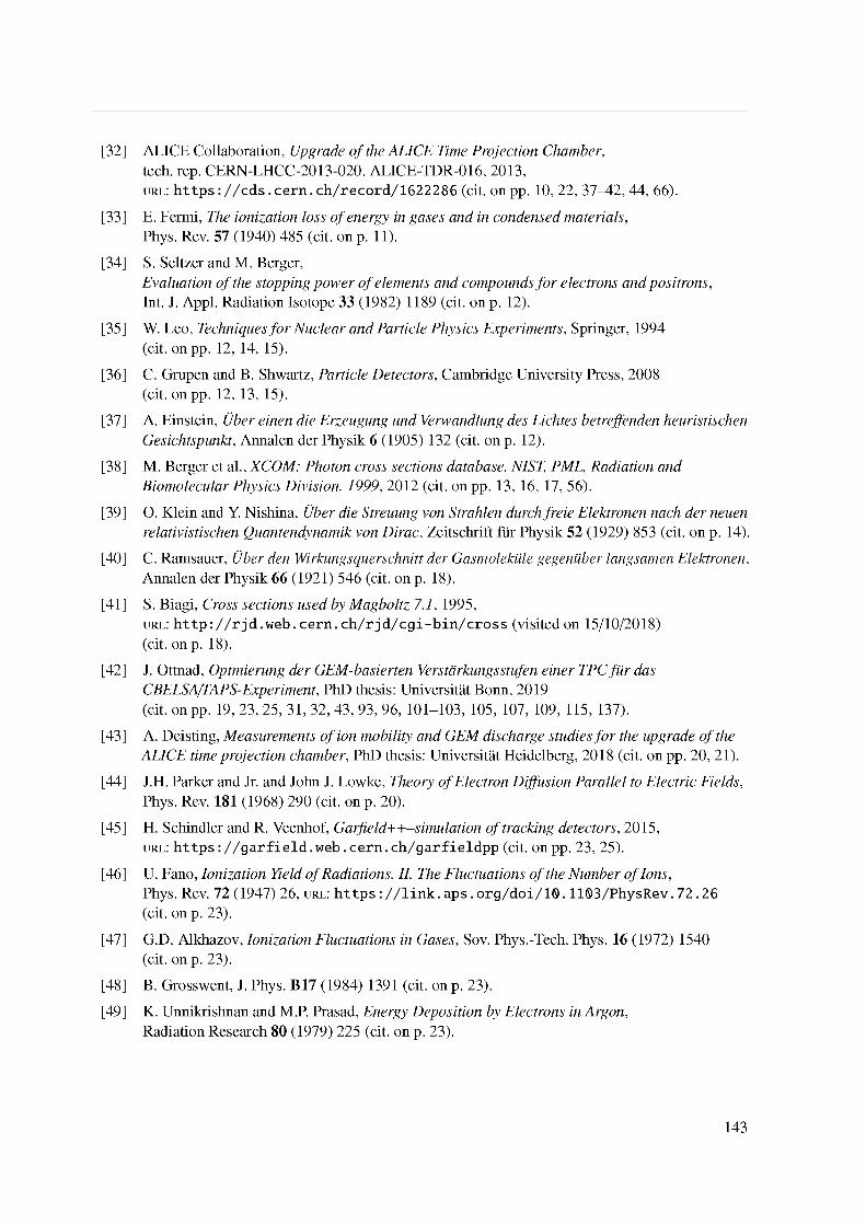
[32] ALICE Collaboration, Upgrade of the ALICE Time Projection Chamber,tech. rep. CERN-LHCC-2013-020. ALICE-TDR-016, 2013,url: https://cds.cern.ch/record/1622286 (cit. on pp. 10, 22, 37-42, 44, 66).
[33] E. Fermi, The ionization loss of energy in gases and in condensed materials, Phys. Rev. 57 (1940) 485 (cit. on p. . 11)
[34] S. Seltzer and M. Berger,Evaluation of the stopping power of elements and compounds for electrons and positrons, Int. J. Appl. Radiation Isotope 33 (1982) 1189 (cit. on p. 12).
[35] W. Leo, Techniques for Nuclear and Particle Physics Experiments, Springer, 1994 (cit. on pp. . 12, 14, 15)
[36] C. Grupen and B. Shwartz, Particle Detectors, Cambridge University Press, 2008 (cit. on pp. . 12, 13, 15)
[37] A. Einstein, Uber einen die Erzeugung und Verwandlung des Lichtes betreffenden heuristischen Gesichtspunkt, Annalen der Physik 6 (1905) 132 (cit. on p. . 12)
[38] M. Berger et al., XCOM: Photon cross sections database. NIST, PML, Radiation and Biomolecular Physics Division. 1999, 2012 (cit. onpp. . 13, 16, 17, 56)
[39] O. Klein and Y. Nishina, Uber die Streuung von Strahlen durch freie Elektronen nach der neuen relativistischen Quantendynamik von Dirac, Zeitschrift fur Physik 52 (1929) 853 (cit. on p. . 14)
[40] C. Ramsauer, Uber den Wirkungsquerschnitt der Gasmolekule gegenuber langsamen Elektronen, Annalen der Physik 66 (1921) 546 (cit. on p. . 18)
[41] S. Biagi, Cross sections used by Magboltz 7.1, 1995,url: http://rjd.web.cern.ch/rjd/cgi-bin/cross (visited on 15/10/2018) (cit. on p. 18).
[42] J. Ottnad, Optmierung der GEM-basierten Verstarkungsstufen einer TPC fur das CBELSA/TAPS-Experiment, PhD thesis: Universitat Bonn, 2019(cit. on pp. 19, 23, 25, 31, 32, 43, 93, 96, 101-103, 105, 107, 109, 115, 137).
[43] A. Deisting, Measurements of ion mobility and GEM discharge studies for the upgrade of the ALICE time projection chamber, PhD thesis: Universitat Heidelberg, 2018 (cit. on pp. . 20, 21)
[44] J.H. Parker and Jr. and John J. Lowke, Theory of Electron Diffusion Parallel to Electric Fields, Phys. Rev. 181 (1968) 290 (cit. on p. . 20)
[45] H. Schindler and R. Veenhof, Garfield++-simulation of tracking detectors, 2015, url: (cit. onpp. . https://garfield.web.cern.ch/garfieldpp 23, 25)
[46] U. Fano, Ionization Yield of Radiations. II. The Fluctuations of the Number of Ions, url:
(cit. on p. .Phys. Rev. 72 (1947) 26, https://link.aps.org/doi/10.1103/PhysRev.72.26
23)
[47] G.D. Alkhazov, Ionization Fluctuations in Gases, Sov. Phys.-Tech. Phys. 16 (1972) 1540 (cit. on p. . 23)
[48] B. Grosswent, J. Phys. B17 (1984) 1391 (cit. on p. . 23)
[49] K. Unnikrishnan and M.P. Prasad, Energy Deposition by Electrons in Argon, Radiation Research 80 (1979) 225 (cit. on p. . 23)
143
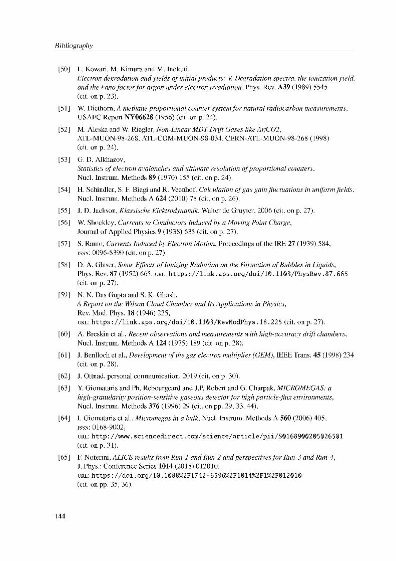
Bibliography
[50] L. Kowari, M. Kimura and M. Inokuti,Electron degradation and yields of initial products: V. Degradation spectra, the ionization yield, and the Fano factor for argon under electron irradiation, Phys. Rev. A39 (1989) 5545 (cit. on p. 23).
[51] W. Diethorn, A methane proportional counter system for natural radiocarbon measurements, USAEC Report NY06628 (1956) (cit. on p. . 24)
[52] M. Aleska and W. Riegler, Non-Linear MDT Drift Gases like Ar/CO2,ATL-MUON-98-268, ATL-COM-MUON-98-034, CERN-ATL-MUON-98-268 (1998) (cit. on p. 24).
[53] G. D. Alkhazov,Statistics of electron avalanches and ultimate resolution of proportional counters, Nucl. Instrum. Methods 89 (1970) 155 (cit. on p. 24).
[54] H. Schindler, S. F. Biagi and R. Veenhof, Calculation of gas gain fluctuations in uniform fields, Nucl. Instrum. Methods A 624 (2010) 78 (cit. on p. . 26)
[55] J. D. Jackson, Klassische Elektrodynamik, Walter de Gruyter, 2006 (cit. on p. . 27)
[56] W. Shockley, Currents to Conductors Induced by a Moving Point Charge, Journal of Applied Physics 9 (1938) 635 (cit. on p. . 27)
[57] S. Ramo, Currents Induced by Electron Motion, issn: 0096-8390 (cit. on p. .
Proceedings of the IRE 27 (1939) 584, 27)
[58] D. A. Glaser, Some Effects of Ionizing Radiation on the Formation of Bubbles in Liquids, url:
(cit. on p. .Phys. Rev. 87 (1952) 665, https://link.aps.org/doi/10.1103/PhysRev.87.665
27)
[59] N. N. Das Gupta and S. K. Ghosh,A Report on the Wilson Cloud Chamber and Its Applications in Physics,Rev. Mod. Phys. 18 (1946) 225,url: https://link.aps.org/doi/10.1103/RevModPhys.18.22 5 (cit. onp. 27).
[60] A. Breskin et al., Recent observations and measurements with high-accuracy drift chambers, Nucl. Instrum. Methods A 124 (1975) 189 (cit. on p. . 28)
[61] J. Benlloch et al., Development of the gas electron multiplier (GEM), IEEE Trans. 45 (1998) 234 (cit. on p. . 28)
[62] J. Ottnad, personal communication, 2019 (cit. on p. . 30)
[63] Y. Giomataris and Ph. Rebourgeard and J.P. Robert and G. Charpak, MICROMEGAS: a high-granularity position-sensitive gaseous detector for high particle-flux environments, Nucl. Instrum. Methods 376 (1996) 29 (cit. on pp. . 29, 33, 44)
[64] I. Giomataris et al., Micromegas in a bulk, issn: 0168-9002,
Nucl. Instrum. Methods A 560 (2006) 405,
url: http://www.sciencedirect.com/science/article/pii/S0168900205026501 (cit. on p. 31).
[65] F. Noferini, ALICE results from Run-1 and Run-2 and perspectives for Run-3 and Run-4,J. Phys.: Conference Series 1014 (2018) 012010, url: https://doi.org/10.1088%2F1742-6596%2F1014%2F1%2F012010 (cit. on pp. 35, 36).
144
[66] L. Cifarelli et al., Insights from the ALICE quark-gluon coloured world at the LHC, (cit. on p. .Riv. Nuovo Cim. 39 (2016) 1 35)
[67] R. Hanbury Brown and R. Twiss, Nature 178 (1956) 1046 (cit. on p. . 35)
[68] K. Aamodt et al.,Two-pion Bose-Einstein correlations in central Pb-Pb collisions at sNN=2.76 TeV,Phys. Lett. B 696 (2011) 328, issn: 0370-2693, url: http://www.sciencedirect.com/science/article/pii/S0370269310014565 (cit. on pp. 35, 36).
[69] B. Abelev et al., Transverse Momentum Distribution and Nuclear Modification Factor of Charged Particles in p+Pb Collisions at psNN=5.02 TeV, url: (cit. onp. .
Phys. Rev. Lett. 110 (2013) 082302, https://link.aps.org/doi/10.1103/PhysRevLett.110.082 302 36)
[70] R.A. Bertens, Anisotropic flow of inclusive and identified particles in Pb-Pb collisions at sNN=5.02 TeV with ALICE, The 26th International Conference on Ultra-relativistic Nucleus-Nucleus Collisions: Quark Matter 2017, issn: 0375-9474,
Nucl. Phys. A 967 (2017) 385,
url: http://www.sciencedirect.com/science/article/pii/S0375947417300969 (cit. on p. 37).
[71] ALICE collaboration, Upgrade of the ALICE Experiment: Letter of Intent, tech. rep. CERN-LHCC-2012-012. LHCC-I-022. ALICE-UG-002, CERN, 2012, url: (cit. onp. . http://cds.cern.ch/record/1475243 36)
[72] ALICE collaboration,Technical Design Report for the Upgrade of the ALICE Inner Tracking System, tech. rep. CERN-LHCC-2013-024. ALICE-TDR-017, 2013, url: http://cds.cern.ch/record/162 5842 (cit. onpp. 37, 38).
[73] ALICE collaboration, The ALICE experiment at the CERN LHC, Journal of Instrumentation S08002 (2008) (cit. on p. . 37)
[74] L3 collaboration, The construction of the L3 experiment, Nucl. Instrum. Methods 289 (1990) 35 (cit. on p. . 38)
[75] ALICE collaboration, Technical Design Report for the Muon Forward Tracker, tech. rep. CERN-LHCC-2015-001. ALICE-TDR-018, 2015,url: https://cds.cern.ch/record/1981898 (cit. onp. 38).
[76] P. Antonioli, A. Kluge and W. Riegler, Upgrade of the ALICE Readout and Trigger System, tech. rep. CERN-LHCC-2013-019. ALICE-TDR-015, 2013,url: https://cds.cern.ch/record/1603472 (cit. onp. 38).
[77] A. Tauro, ALICE Schematics (ALICE-PHO-SKE-2017-001), 2017 (cit. on p. . 39)
[78] D. Nygren, The Time Projection Chamber,Lawrence Berkeley National Laboratory LBNL Report: LBL-8367 (1978) (cit. on p. 38).
[79] ALICE collaboration, ALICE Time Projection Chamber: Technical Design Report, tech. rep., 2000, url: (cit. on pp. . https://cds.cern.ch/record/451098 38, 40, 41)
[80] J. Alme et al., The ALICE TPC, a large 3-dimensional tracking device with fast readout for ultra-high multiplicity events, issn: 0168-9002, url: (cit. on p. .
Nucl. Instrum. Methods A 622 (2010) 316, http://www.sciencedirect.com/science/article/pii/S0168900210008910
39)
145
Bibliography
[81] F. Bohmer et al., Simulation of space-charge ejfects in an ungated GEM-based TPC, Nucl. Instrum. Methods A 719 (2013) 101 (cit. on p. . 39)
[82] S. Rossegger, Simulation and Calibration of the ALICE Time-Projection Chamber including innovative Space Charge Calculations, PhD thesis: Graz University of Technology, 2009 (cit. on p. . 39)
[83] B. Ketzer,A time projection chamber for high-rate experiments: Towards an upgrade of the ALICE TPC, Nucl. Instrum. Methods A 732 (2013) 237 (cit. on pp. 41, 44).
[84] M. Ball et al., Ion backflow studies for the ALICE TPC upgrade with GEMs, Journal of Instrumentation C04025 (2014) (cit. on p. . 41)
[85] ALICE Collaboration, Addendum to the Technical Design Report for the Upgrade of the ALICE Time Projection Chamber, tech. rep. CERN-LHCC-2015-002. ALICE-TDR-016-ADD-1, 2015, url: (cit. on pp. . https://cds.cern.ch/record/1984329 41, 43-45)
[86] ALICE Collaboration,Readout Chambers Production, Part 1: Final Readout Chambers characterization, 2017, url: https://indico.cern.ch/event/617818/contributions/2493327/ attachments/1422943/2186698/gasik_PRR_PART_I.pdf (visited on 11/12/2018) (cit. on p. 43).
[87] P. Gasik, Discharge probability studies with multi-GEM detectors for the ALICE TPC Upgrade, Submitted to: PoS (2018), [PoSMPGD2017,031(2017)],arXiv: 1807.02979 [physics.ins-det] (cit. onp. 43).
[88] S. Bachmann et al., Discharge studies and prevention in the gas electron multiplier (GEM), issn: 0168-9002,Nucl. Instrum. Methods A 479 (2002) 294,
url: http://www.sciencedirect.com/science/article/pii/S0168900201009317 (cit. on p. 43).
[89] J. Paschek, Vergleich von Simulationen und Messungen hinsichtlich des Verstarkungsverhalten von GEMs am Beispiel der ALICE-TPC, B.Sc. thesis: Universitat Bonn, 2019 (cit. on p. . 43)
[90] G. Bencivenni et al.,Performance of a triple-GEM detector for high rate charged particle triggering, Nucl. Instrum. Methods A 494 (2002) 156 (cit. on p. 43).
[91] L. Fabbietti et al., The PANDA GEM-based TPCprototype, Nucl. Instrum. Methods A 628 (2011) 204 (cit. on p. . 44)
[92] M. Ball et al., Technical Design Study for the PANDA Time Projection Chamber, GEM-TPC Collaboration, arXiv:1207.0013 [physics.ins-det] (2012) (cit. onp. . 44)
[93] P. Colas et al., Ion backflow in the Micromegas TPC for the future linear collider, Nucl. Instrum. Methods A 535 (2004) 226 (cit. on p. . 44)
[94] S. Kane et al., A study of Micromegas with preamplification with a single GEM, Proceedings of the 7th International Conference on ICATPP-7, World Scientific (2002) 694 (cit. on p. . 44)
[95] G. Charles et al., Discharge studies in Micromegas detectors in low energy hadron beams, Nucl. Instrum. Methods A 648 (2011) 174 (cit. on p. . 44)
146
[96] M. Vandenbroucke,Discharge reduction technologies for Micromegas detectors in high hadron flux environments, 2nd International Conference on Micro Pattern Gaseous Detectors (2012) (cit. on p. 44).
[97] C. Hoppner,First Measurement of the Cross Section for the Production of Hadrons with High Transverse Momenta at COMPASS, and Developments for Particle Tracking in High-Rate Experiments, PhD thesis: Tech. U. Munich, 2012 (cit. on p. 47).
[98] A. Bugl, Weiterentwicklung und Charakterisierung von Hochspannungs-Picoamperemetern, B.Sc. thesis: Techn. Univ. Munchen, 2013 (cit. on p. . 47)
[99] R.B.J. Rodel,Entwicklung eines voll automatisierten Kalibrationsprozesses fur Picoamperemeter, B.Sc. thesis: Universitat Bonn, 2016 (cit. on p. 47).
[100] P. Hauer, Study of Charge-Up Processes in Gas Electron Multipliers,M.Sc. thesis: Universitat Bonn, 2017 (cit. on p. 48).
[101] Correia et al., A dynamic method for charging-up calculations: the case of GEM, Journal of Instrumentation 9 (2014) P07025,url: https://doi.org/10.1088%2F1748-0221%2F9%2F07%2Fp0702 5 (cit. onp. 48).
[102] D. Kaiser, Steuerung und Uberwachung einer Zeitprojektionskammer mit GEM-Auslese, PhD thesis: Universitat Bonn, 2014 (cit. on p. . 52)
[103] A. Thompson et al., X-Ray data booklet,Lawrence Berkeley National Laboratory, University of California, 2009 (cit. on pp. 55, 58, 59).
[104] Martin J. Berger, J S. Coursey, M A. Zucker, ESTAR, PSTAR, andASTAR: Computer Programs for Calculating Stopping-Power and Range Tables for Electrons, Protons, and Helium Ions, 1999 (cit. on p. . 56)
[105] J. Yeh and I. Lindau,Atomic subshell photoionization cross sections and asymmetry parameters: 1 < Z < 103, Atomic Data and Nuclear Data Tables 32 (1985) 1, issn: 0092-640X,url: http://www.sciencedirect.com/science/article/pii/0092640X85900166 (cit. on pp. 58, 59).
[106] L. I. Yin, E. Yellin and I. Adler, X-Ray Excited LMM Auger Spectra of Copper, Nickel, and Iron, url:
(cit. on pp. .Journal of Applied Physics 42 (1971) 3595, https://doi.org/10.1063/1.1660775
58, 59)
[107] P. E. Larson,X-ray induced photoelectron and auger spectra of Cu, CuO, Cu2O, and Cu2S thin films, Journal of Electron Spectroscopy and Related Phenomena 4 (1974) 213, issn: 0368-2048, url: http://www.sciencedirect.com/science/article/pii/0368204874800526 (cit. on pp. 58, 59).
[108] S. P. Kowalczyk et al.,L2;3 M45 M45 Auger Spectra of Metallic Copper and Zinc: Theory and Experiment,Phys. Rev. B 8 (6 1973) 2387,url: https://link.aps.org/doi/10.1103/PhysRevB.8.2387 (cit. on pp. 58, 59).
147
Bibliography
[109] E. Antonides, E. C. Janse and G. A. Sawatzky, LMM Auger spectra ofCu, Zn, Ga, and Ge. I.Transition probabilities, term splittings, and effective Coulomb interaction, Phys. Rev. B 15 (4 1977) 1669,url: https://link.aps.org/doi/10.1103/PhysRevB.15.1669 (cit. onpp. 58, 59).
[110] K. Ueda et al., Threshold behaviour of the multiply-charged photoion yields near the Ar K edge, J. Phys. B 24 (1991)605,url: https://doi.org/10.1088%2F0953-4075%2F24%2F3%2F016 (cit. on pp. 58, 59).
[111] S. Aiola et al., Combination of two Gas Electron Multipliers and a Micromegas as gain elements for a time projection chamber, issn: 0168-9002, url: (cit. onpp. .
Nucl. Instrum. Methods A 834 (2016) 149, http://www.sciencedirect.com/science/article/pii/S0168900216308221
67, 68, 71, 72, 120, 121, 123-126, 128)
[112] Nikolai Smirnov, DPG-Fruhjahrstagung, Heidelberg, personal communication, 2015 (cit. on p. . 67)
[113] High Energy Group, Institut fur Kernphysik, Goethe-Universitat, Frankfurt am Main, personal communication, 2018 (cit. on pp. . 68, 71, 127-131)
[114] WeatherOnline Ltd. - Meteorological Services, WeatherOnline,url: https://www.weatheronline.de (visited on 26/03/2019) (cit. on p. 69).
[115] M. Killenberg et al., Modelling and measurement of charge transfer in multiple GEM structures, (cit. on pp. .Nucl. Instrum. Methods A 498 (2003) 369 74, 76, 83, 88)
[116] G. Bencivenni et al., Measurement of GEM parameters with X-rays, (cit. on p. .IEEE Transactions on Nuclear Science 50 (2003) 1297 74)
[117] J. D. Jackson, Classical electrodynamics, 4th ed., Wiley, 1999, isbn: 9780471309321, url: (cit. onpp. . http://cdsweb.cern.ch/record/490457 77, 92)
[118] J. Bloemer, Performance Studies of a Quadruple GEM System and Development of an Electron Transport Model for the ALCIE TPC Upgrade,M.Sc. thesis: Technische Universitat Munchen, 2014 (cit. on pp. 93, 135).
[119] R. Veenhof, personal communication, 2019 (cit. on pp. . 115, 127)
[120] ALICE Collaboration, Upgrade of the Online - Offline computing system, tech. rep. CERN-LHCC-2015-006. ALICE-TDR-019, 2015,url: https://cds.cern.ch/record/2011297 (cit. onp. 132).
[121] K. T. McDonald, Conducting Ellipsoid and Circular Disk,Joseph Henry Laboratories, Princeton University, Princeton, NJ 08544 (2002) (cit. on p. 139).
148
APPENDIX A
Appendix
A.1 Source code: Bonn Hybrid Detector
Example C++ source code to calculate the energy resolution, the ion backflow and the total effective gain for the hybrid 2GEM-MM detector (in case of ETF2 = 400 V cm-1). Additional functions are used in order to study the stack in details.
#include "GEMStack.h"
void HybridDetector (){
// Define stack and gas propertiesGEMStack * Detector = new GEMStack();Detector ->SetPhotonEnergy (5900);Detector ->SetGas (GAS_NECO2);Detector ->SetAttachmentFactor (0.04);Detector -> Set Attachment (1);
// Define stack geometry and potentialsDetector ->AddVolume(2.6 , 400.0);int GEM1 = Detector ->AddGEM(GEM_ST, 270.0);Detector ->AddVolume(0.2 , 3 000.0);int GEM2 = Detector ->AddGEM(GEM_ST, 350.0);Detector ->AddVolume(0.4 , 400.0);int MM = Detector ->AddGEM(GEM_ST, 370.0);Detector ->AddVolume(0.0 , 0.0);
// Overwrite properties of last "GEM" to those of a MMDetector ->SetGEMElectronCol lection (MM, 0.99);Detector ->SetGEMElectronExtraction (MM, 1.0);Detector ->SetGEMAvalancheIonCollection (MM, 0.99);Detector ->SetGEMAvalancheIonExtraction (MM, 0.01);Detector ->SetGEMAbsGain (MM, 0.02195, - 2.116);Detector ->SetGEMSingleGainFluctuation (MM, 0.8);
// Set models for calculationsDetector ->SetSingleGainFluctuationModel (MODEL_EXP_NOLIMIT);Detector -> SetDriftIonModel( MODEL_DRIFT_ION_CALC);
149
Appendix A Appendix
// Tune total gain and drift ion collection efficiencyDetector -> Set Ab s Gain Scaling Factor (1.0);Detector ->SetDriftIonGEMsDisplacement (52.0);
// Get stack propertiesdouble EnergyResolution = Detector ->GetEnergyResolution ();double IonBackflow = Detector ->GetIonBackflow ();double EffGain = Detector ->GetTotalEffGain ();
// Effective or absolute gain of a single stagedouble EffGainGEM1 = Detector ->GetGEMEffGain (GEM1);double AbsGainGEM1 = Detector ->GetGEMAbsGain (GEM1);
/ / Epsilon co n trib u tio n of second GEMdouble EpsilonGEM2 = Detector ->GetGEMEpsilonContribution (GEM2);
/ / A simp le way to p lo t the effi c i e n c i e s of the fi r s t GEMTCanvas *c = new TCanvas ("c" , "c" ,0 ,0,1024 ,768);Detector ->DrawGEMEfficiencyCurves (GEM1, c, 1, 1, 1);
}
A.2 Source code: S-LP-LP-S configuration with the ALICE O2 framework
using namespace o2::TPC;
#include <vector>
void CalcStackSettings () {
ModelGEM Model ;
std : : array <int , 4> mGeometry ;std :: array < float, 5> mDistance;std : : array <float , 4> mPotential ;std : : array <float , 5> mElectricField ;
mGeometry = { { 0 , 2 , 2 , 0 } } ;mDistance = { { 4.f, 0.2f, 0.2f, 0.2f, 0.2f } };mPotential = { { 225.f, 285.f, 280.f, 349.f } };mElectricField = { { 0.4f, 4.f, 4.f, 0.1f, 4.f } };
Model. set Attachment (0.06);Model. setAbsGainScalingFactor(1.53);
Model. setStackProperties (mGeometry , mDistance, mPotential, mElectricField);
std::cout << Model. getStackEnergyResolution ()* 100.0 << std :: endl;std : : cout << Model . getStackEffectiveGain () << std : : endl ;
}
150
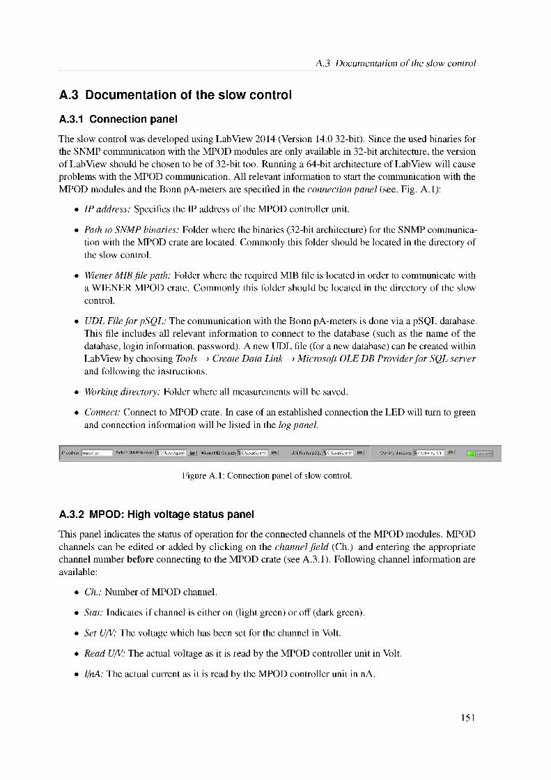
A.3 Documentation of the slow control
A.3 Documentation of the slow control
A.3.1 Connection panel
The slow control was developed using LabView 2014 (Version 14.0 32-bit). Since the used binaries for the SNMP communication with the MPOD modules are only available in 32-bit architecture, the version of LabView should be chosen to be of 32-bit too. Running a 64-bit architecture of LabView will cause problems with the MPOD communication. All relevant information to start the communication with the MPOD modules and the Bonn pA-meters are specified in the connection panel (see. Fig. A.1):
• IP address: Specifies the IP address of the MPOD controller unit.
• Path to SNMP binaries: Folder where the binaries (32-bit architecture) for the SNMP communication with the MPOD crate are located. Commonly this folder should be located in the directory of the slow control.
• Wiener MIB file path: Folder where the required MIB file is located in order to communicate with a WIENER MPOD crate. Commonly this folder should be located in the directory of the slow control.
• UDL File for pSQL: The communication with the Bonn pA-meters is done via a pSQL database. This file includes all relevant information to connect to the database (such as the name of the database, login information, password). A new UDL file (for a new database) can be created within LabView by choosing Tools ! Create Data Link ! Microsoft OLE DB Provider for SQL server and following the instructions.
• Working directory: Folder where all measurements will be saved.
• Connect: Connect to MPOD crate. In case of an established connection the LED will turn to green and connection information will be listed in the log panel.
Figure A.1: Connection panel of slow control.
A.3.2 MPOD: High voltage status panel
This panel indicates the status of operation for the connected channels of the MPOD modules. MPOD channels can be edited or added by clicking on the channel field (Ch.) and entering the appropriate channel number before connecting to the MPOD crate (see A.3.1). Following channel information are available:
• Ch.: Number of MPOD channel.
• Stat: Indicates if channel is either on (light green) or off (dark green).
• Set UV: The voltage which has been set for the channel in Volt.
• Read UV: The actual voltage as it is read by the MPOD controller unit in Volt.
• I/nA: The actual current as it is read by the MPOD controller unit in nA.
151
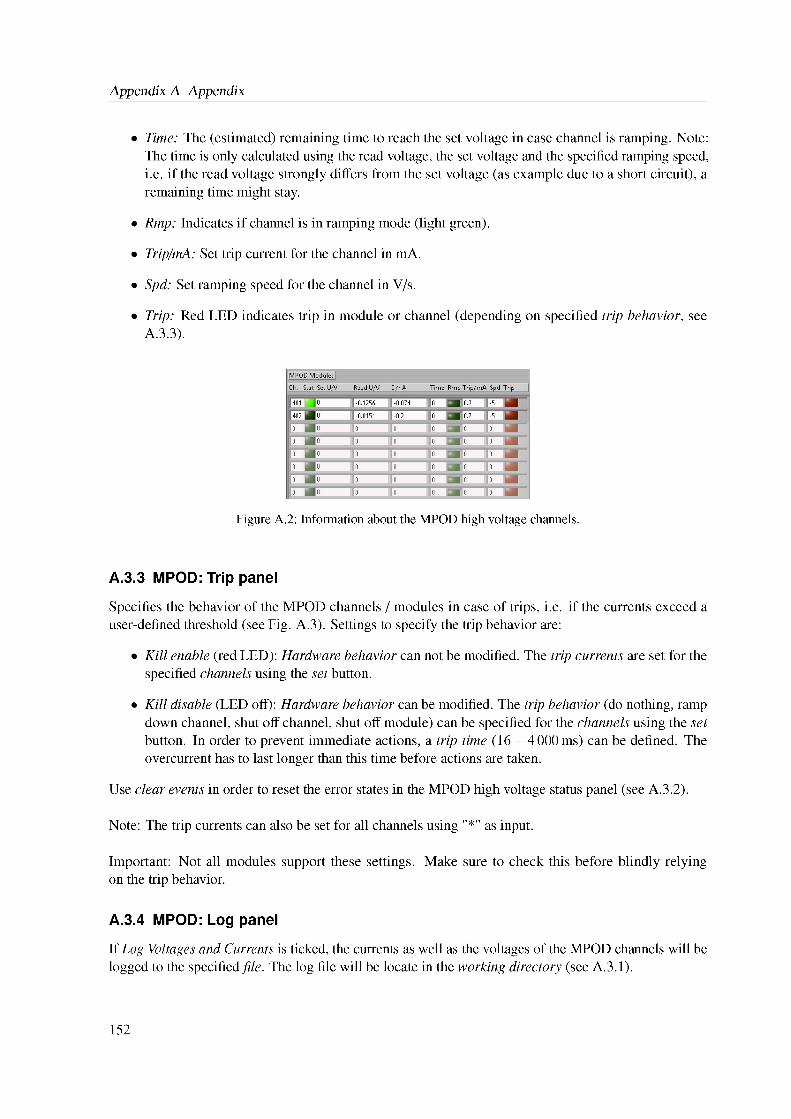
Appendix A Appendix
• Time: The (estimated) remaining time to reach the set voltage in case channel is ramping. Note: The time is only calculated using the read voltage, the set voltage and the specified ramping speed, i.e. if the read voltage strongly differs from the set voltage (as example due to a short circuit), a remaining time might stay.
• Rmp: Indicates if channel is in ramping mode (light green).
• Trip/mA: Set trip current for the channel in mA.
• Spd: Set ramping speed for the channel in V/s.
• Trip: Red LED indicates trip in module or channel (depending on specified trip behavior, see .A.3.3)
Figure A.2: Information about the MPOD high voltage channels.
A.3.3 MPOD: Trip panel
Specifies the behavior of the MPOD channels / modules in case of trips, i.e. if the currents exceed a user-defined threshold (see Fig. A.3). Settings to specify the trip behavior are:
• Kill enable (red LED): Hardware behavior can not be modified. The trip currents are set for the specified channels using the set button.
152
• Kill disable (LED off): Hardware behavior can be modified. The trip behavior (do nothing, ramp down channel, shut off channel, shut off module) can be specified for the channels using the set button. In order to prevent immediate actions, a trip time (16 - 4000 ms) can be defined. The overcurrent has to last longer than this time before actions are taken.
Use clear events in order to reset the error states in the MPOD high voltage status panel (see A.3.2).
Note: The trip currents can also be set for all channels using "*" as input.
Important: Not all modules support these settings. Make sure to check this before blindly relying on the trip behavior.
A.3.4 MPOD: Log panel
If Log Voltages and Currents is ticked, the currents as well as the voltages of the MPOD channels will be logged to the specified file. The log file will be locate in the working directory (see A.3.1).
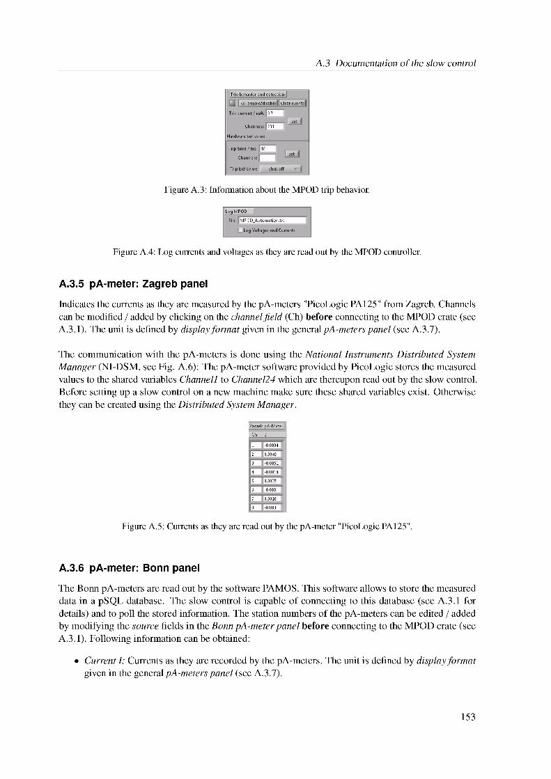
A.3 Documentation of the slow control
Figure A.3: Information about the MPOD trip behavior.
Figure A.4: Log currents and voltages as they are read out by the MPOD controller.
A.3.5 pA-meter: Zagreb panel
Indicates the currents as they are measured by the pA-meters "PicoLogic PA125" from Zagreb. Channels can be modified / added by clicking on the channel field (Ch) before connecting to the MPOD crate (see A.3.1). The unit is defined by display format given in the general pA-meters panel (see A.3.7).
The communication with the pA-meters is done using the National Instruments Distributed System Manager (NI-DSM, see Fig. A.6): The pA-meter software provided by PicoLogic stores the measured values to the shared variables Channel1 to Channel24 which are thereupon read out by the slow control. Before setting up a slow control on a new machine make sure these shared variables exist. Otherwise they can be created using the Distributed System Manager.
Figure A.5: Currents as they are read out by the pA-meter "PicoLogic PA125".
A.3.6 pA-meter: Bonn panel
The Bonn pA-meters are read out by the software PAMOS. This software allows to store the measured data in a pSQL database. The slow control is capable of connecting to this database (see A.3.1 for details) and to poll the stored information. The station numbers of the pA-meters can be edited / added by modifying the source fields in the Bonn pA-meter panel before connecting to the MPOD crate (see A.3.1). Following information can be obtained:
• Current I: Currents as they are recorded by the pA-meters. The unit is defined by display format given in the general pA-meters panel (see A.3.7).
153
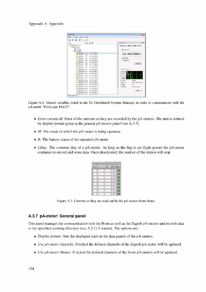
Appendix A Appendix
Figure A.6: Shared variables listed in the NI Distributed System Manager in order to communicate with the pA-meter "PicoLogic PA125".
• Error current dl: Error of the currents as they are recorded by the pA-meters. The unit is defined by display format given in the general pA-meters panel (see . A.3.7)
• M: The mode in which the pA-meter is being operated.
• B: The battery status of the operated pA-meter.
• Cflag: The continue flag of a pA-meter. As long as the flag is set (light green) the pA-meter continues to record and store data. Once deactivated, the readout of the station will stop.
Figure A.7: Currents as they are read out by the pA-meters from Bonn.
A.3.7 pA-meter: General panel
This panel manages the communication with the Bonn as well as the Zagreb pA-meters and records data to the specified working directory (see A.3.1) if wanted. The options are:
• Display format: Sets the displayed units in the data panels of the pA-meters.
• Use pA-meter (Zagreb): If ticked the defined channels of the Zagreb pA-meter will be updated.
• Use pA-meter (Bonn): If ticked the defined channels of the Bonn pA-meters will be updated.
154
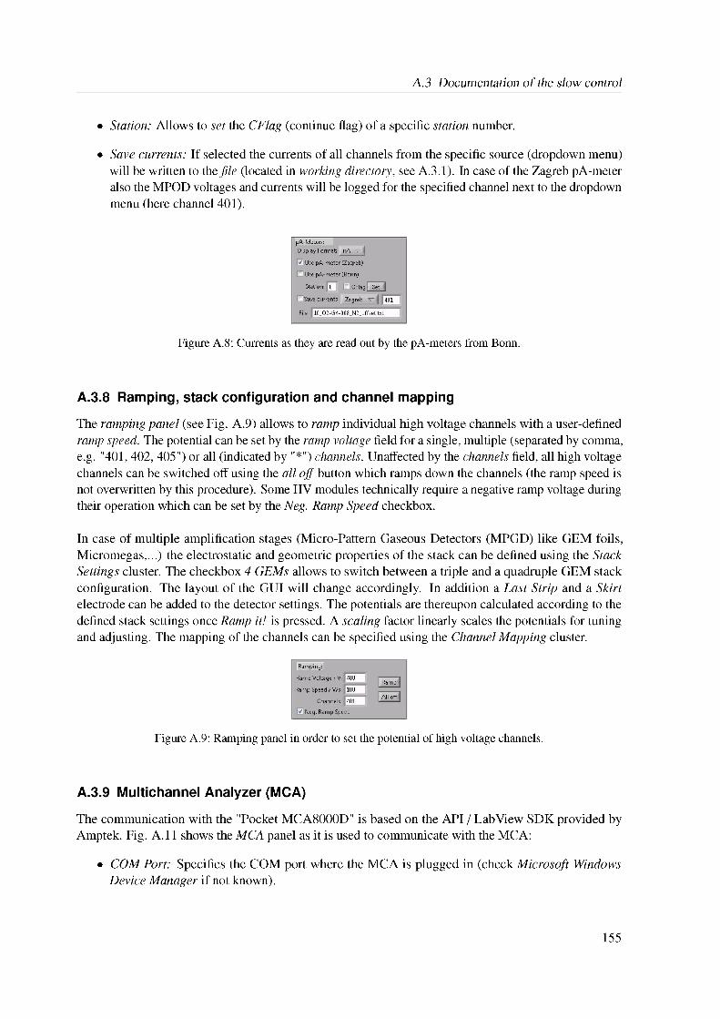
A.3 Documentation of the slow control
• Station: Allows to set the CFlag (continue flag) of a specific station number.
• Save currents: If selected the currents of all channels from the specific source (dropdown menu) will be written to the file (located in working directory, see . In case of the Zagreb pA-meter also the MPOD voltages and currents will be logged for the specified channel next to the dropdown menu (here channel 401).
A.3.1)
Figure A.8: Currents as they are read out by the pA-meters from Bonn.
A.3.8 Ramping, stack configuration and channel mapping
The ramping panel (see Fig. A.9) allows to ramp individual high voltage channels with a user-defined ramp speed. The potential can be set by the ramp voltage field for a single, multiple (separated by comma, e.g. "401, 402, 405") or all (indicated by "*") channels. Unaffected by the channels field, all high voltage channels can be switched off using the all off button which ramps down the channels (the ramp speed is not overwritten by this procedure). Some HV modules technically require a negative ramp voltage during their operation which can be set by the Neg. Ramp Speed checkbox.
• COM Port: Specifies the COM port where the MCA is plugged in (check Microsoft Windows Device Manager if not known).
In case of multiple amplification stages (Micro-Pattern Gaseous Detectors (MPGD) like GEM foils, Micromegas,...) the electrostatic and geometric properties of the stack can be defined using the Stack Settings cluster. The checkbox 4 GEMs allows to switch between a triple and a quadruple GEM stack configuration. The layout of the GUI will change accordingly. In addition a Last Strip and a Skirt electrode can be added to the detector settings. The potentials are thereupon calculated according to the defined stack settings once Ramp it! is pressed. A scaling factor linearly scales the potentials for tuning and adjusting. The mapping of the channels can be specified using the Channel Mapping cluster.
Figure A.9: Ramping panel in order to set the potential of high voltage channels.
A.3.9 Multichannel Analyzer (MCA)
The communication with the "Pocket MCA8000D" is based on the API / LabView SDK provided by Amptek. Fig. A.11 shows the MCA panel as it is used to communicate with the MCA:
155
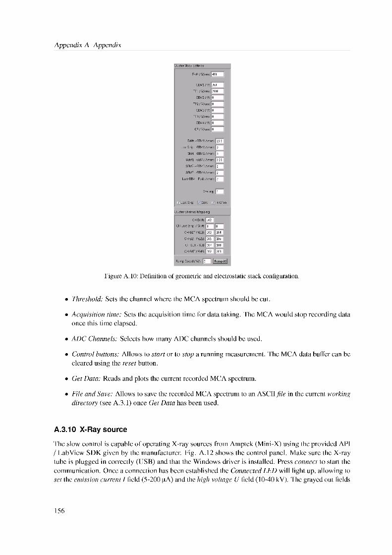
Appendix A Appendix
Figure A.10: Definition of geometric and electrostatic stack configuration.
• Threshold: Sets the channel where the MCA spectrum should be cut.
• Acquisition time: Sets the acquisition time for data taking. The MCA would stop recording data once this time elapsed.
• ADC Channels: Selects how many ADC channels should be used.
• Control buttons: Allows to start or to stop a running measurement. The MCA data buffer can be cleared using the reset button.
• Get Data: Reads and plots the current recorded MCA spectrum.
• File and Save: Allows to save the recorded MCA spectrum to an ASCII file in the current working directory (see once Get Data has been used. A.3.1)
A.3.10 X-Ray source
The slow control is capable of operating X-ray sources from Amptek (Mini-X) using the provided API / LabView SDK given by the manufacturer. Fig. A.12 shows the control panel. Make sure the X-ray tube is plugged in correctly (USB) and that the Windows driver is installed. Press connect to start the communication. Once a connection has been established the Connected LED will light up, allowing to set the emission current I field (5-200 pA) and the high voltage U field (10-40 kV). The grayed out fields
156
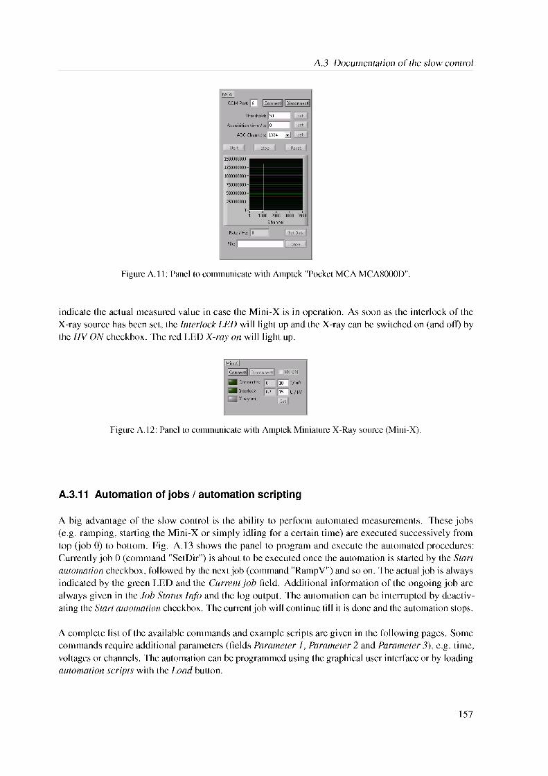
A.3 Documentation of the slow control
Figure A.11: Panel to communicate with Amptek "Pocket MCA MCA8000D".
indicate the actual measured value in case the Mini-X is in operation. As soon as the interlock of the X-ray source has been set, the Interlock LED will light up and the X-ray can be switched on (and off) by the HV ON checkbox. The red LED X-ray on will light up.
Figure A.12: Panel to communicate with Amptek Miniature X-Ray source (Mini-X).
A.3.11 Automation of jobs I automation scripting
A big advantage of the slow control is the ability to perform automated measurements. These jobs (e.g. ramping, starting the Mini-X or simply idling for a certain time) are executed successively from top (job 0) to bottom. Fig. A.13 shows the panel to program and execute the automated procedures: Currently job 0 (command "SetDir") is about to be executed once the automation is started by the Start automation checkbox, followed by the next job (command "RampV") and so on. The actual job is always indicated by the green LED and the Current job field. Additional information of the ongoing job are always given in the Job Status Info and the log output. The automation can be interrupted by deactivating the Start automation checkbox. The current job will continue till it is done and the automation stops.
A complete list of the available commands and example scripts are given in the following pages. Some commands require additional parameters (fields Parameter 1, Parameter 2 and Parameter 3), e.g. time, voltages or channels. The automation can be programmed using the graphical user interface or by loading automation scripts with the Load button.
157
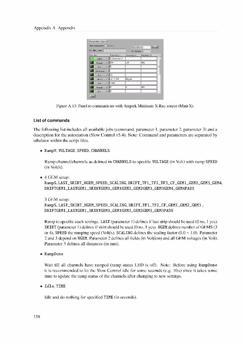
Appendix A Appendix
Figure A.13: Panel to communicate with Amptek Miniature X-Ray source (Mini-X).
List of commands
The following list includes all available jobs (command, parameter 1, parameter 2, parameter 3) and a description for the automation (Slow Control v5.4). Note: Command and parameters are separated by tabulator within the script files.
• RampV,VOLTAGE,SPEED,CHANNELS
Ramp channel/channels as defined in CHANNELS to specific VOLTAGE (in Volt) with ramp SPEED (in Volt/s).
• 4 GEM setup:RampS,LAST_SKIRT_NGEM_SPEED_SCALING,DRIFT_TF1_TF2_TF3_CF_GEM1_GEM2_GEM3_GEM4, DRIFTGEM1_LASTGEM1_SKIRTGEM1_GEM1GEM2_GEM2GEM3_GEM3GEM4_GEM4PADS
3 GEM setup:RampS, LAST_SKIRT_NGEM_SPEED_SCALING, DRIFT_TF1_TF2_CF_GEM1_GEM2_GEM3 , DRIFTGEM1_LASTGEM1_SKIRTGEM1_GEM1GEM2_GEM2GEM3_GEM3PADS
Ramp to specific stack settings. LAST (parameter 1) defines if last strip should be used (0 no, 1 yes). SKIRT (parameter 1) defines if skirt should be used (0 no, 1 yes). NGEM defines number of GEMS (3 or 4), SPEED the ramping speed (Volt/s), SCALING defines the scaling factor (0.0 - 1.0). Parameter 2 and 3 depend on NGEM. Parameter 2 defines all fields (in Volt/cm) and all GEM voltages (in Volt). Parameter 3 defines all distances (in mm).
• RampDone
Wait till all channels have ramped (ramp status LED is off). Note: Before using RampDone it is recommended to let the Slow Control idle for some seconds (e.g. 10 s) since it takes some time to update the ramp status of the channels after changing to new settings.
• Idle, TIME
Idle and do nothing for specified TIME (in seconds).
158

A.3 Documentation of the slow control
• StartC,FILENAME, PAMETER
Starts a currents measurement and saves the data in the file FILENAME (within the working directory). PAMETER defines which pA-meter should be used (i.e. "Zagreb" or "Bonn"). The output format of the saved currents is defined by "Display Format" in the GUI. Note: This command does not activate "Use pA-Meter (...)" option in the GUI. It just defines the path, filename, sets the source and starts the measurement.
• StopC
Stops an ongoing current measurement.
• Stop
End of the automation script.
• SetCFlag, STATIONNO, FLAG
Set the continue FLAG (0 or 1) of a Bonn pA-meter with station number STATIONNO.
• SetDir,DIR
Set the working directory to DIR .Note: The path should not end with "\", e.g. "C:\working_directory" is correct.
• GoTo, JOBNO
Jump to a specific job with number JOBNO (counting starts with 0 for the first job).
• MiniXOn
Switches Mini-X on (requires a connected device and a closed interlock, otherwise this command will be skipped).
• MiniXOff
Switches Mini-X off (requires a connected device and a closed interlock, otherwise this command will be skipped).
• MiniXSetUI, VOLTAGE, CURRENT
Set the high VOLTAGE (value between 10 - 40 kV) and the emission CURRENT (value between 5 - 200 ^A). This requires a connected device and a closed interlock, otherwise this command will be skipped. This command can only be executed when the HV is switched off.
• MPODLogStart, FILENAME
Start logging of MPOD voltages and currents to file specified by FILENAMEin current working directory.
159
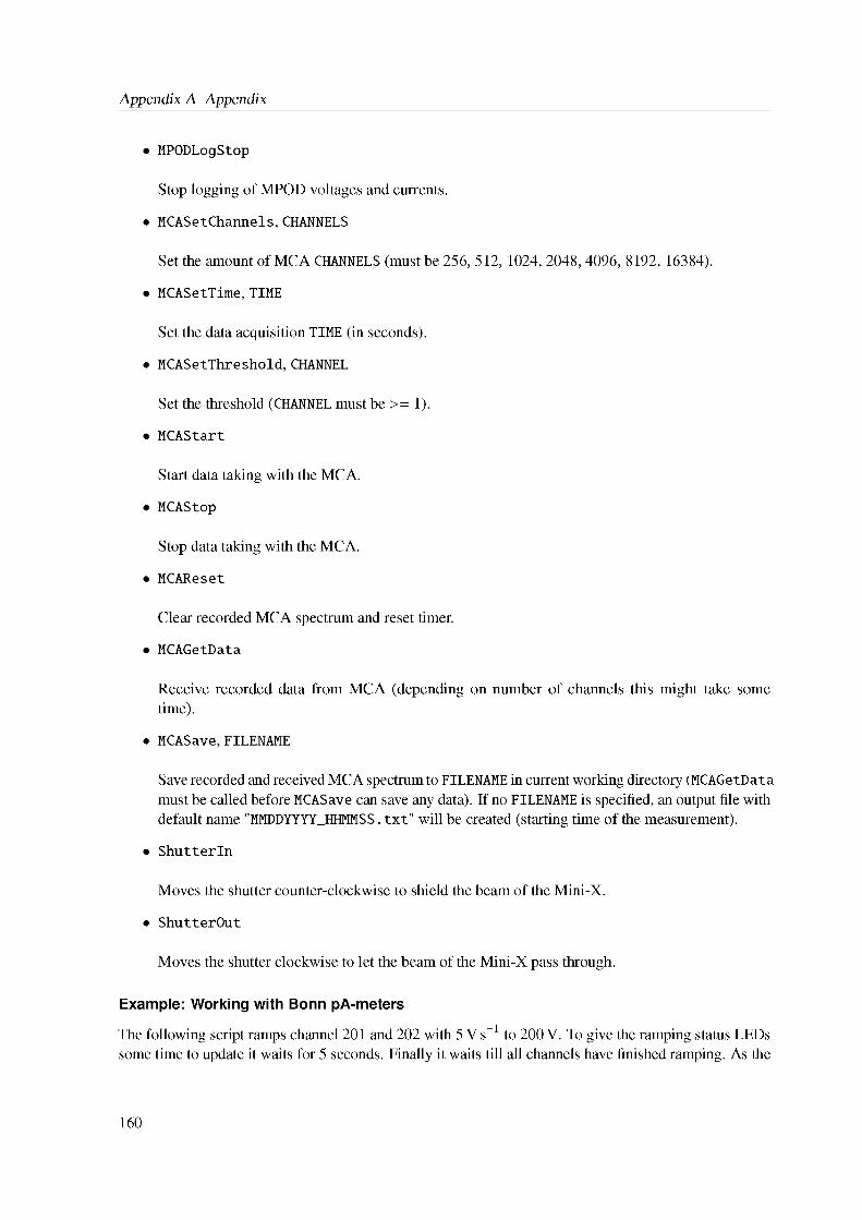
Appendix A Appendix
• MPODLogStop
Stop logging of MPOD voltages and currents.
• MCASetChannels,CHANNELS
Set the amount of MCA CHANNELS (must be 256,512, 1024, 2048,4096, 8192, 16384).
• MCASetTime, TIME
Set the data acquisition TIME (in seconds).
• MCASetThreshold, CHANNEL
Set the threshold (CHANNEL must be >= 1).
• MCAStart
Start data taking with the MCA.
• MCAStop
Stop data taking with the MCA.
• MCAReset
Clear recorded MCA spectrum and reset timer.
• MCAGetData
Receive recorded data from MCA (depending on number of channels this might take some time).
• MCASave,FILENAME
Save recorded and received MCA spectrum to FILENAME in current working directory (MCAGetData must be called before MCASave can save any data). If no FILENAME is specified, an output file with default name "MMDDYYYY_HHMMSS.txt" will be created (starting time of the measurement).
• ShutterIn
Moves the shutter counter-clockwise to shield the beam of the Mini-X.
• ShutterOut
Moves the shutter clockwise to let the beam of the Mini-X pass through.
Example: Working with Bonn pA-meters
The following script ramps channel 201 and 202 with 5 V s-1 to 200 V. To give the ramping status LEDs some time to update it waits for 5 seconds. Finally it waits till all channels have finished ramping. As the
160
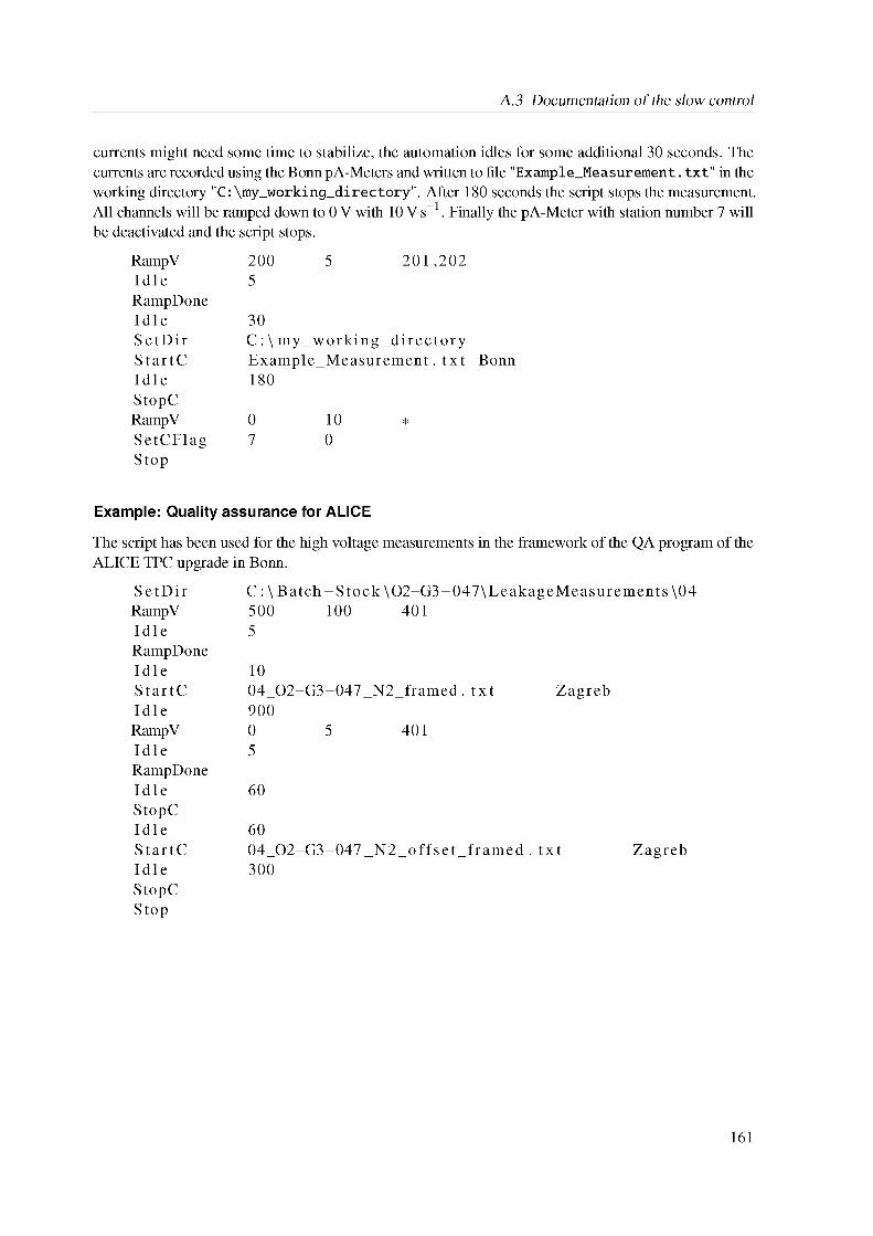
A.3 Documentation of the slow control
currents might need some time to stabilize, the automation idles for some additional 30 seconds. The currents are recorded using the Bonn pA-Meters and written to file "Example_Measurement.txt" in the working directory "C:\my_working_directory". After 180 seconds the script stops the measurement. All channels will be ramped down to 0 V with 10 V s-1. Finally the pA-Meter with station number 7 will be deactivated and the script stops.
RampV 200 5 201 ,202IdleRampDone
5
Idle 30SetDir C: \ my_working_directoryStartC Example_Measurement.txt BonnIdleStopC
180
RampV 0 10 *SetCFlagStop
70
Example: Quality assurance for ALICE
The script has been used for the high voltage measurements in the framework of the QA program of the ALICE TPC upgrade in Bonn.
SetDir RampV Idle RampDone Idle StartC Idle RampV Idle RampDone Idle StopC Idle StartC Idle StopC Stop
C : \ Batch - Stock \ O2-G3 - 047 \ LeakageMeasurements \ 04 500 100 4015
10 04_O2-G3-047_N2_framed . txt Zagreb900 0 5 4015
60
60 04_O2-G3-047_N2_offset_framed . txt Zagreb300
161


List of Figures
1.1 Measurements of the structure function F2 for the proton and the ratio of the structurefunctions F1 and F2 (crosscheck of the Callan-Gross relation)........................................... 2
1.2 Summary of measurements for the strong coupling constant as(Q) [10]............................ 31.3 The Standard Model of Elementary Particles [11]................................................................. 41.4 Calculated pressure p, energy density e and entropy density ,v in QCD as a function of the
temperature (plot from [16]). Solid lines indicate results obtained from hadron resonancegas (HRG) model calculations [17].......................................................................................... 5
1.5 Simplified schematic of the QCD phase diagram................................................................... 51.6 Fourier coefficient v2 as a function of the transverse momentum pt for different particle
species within Au-Au collision at RHIC [20]......................................................................... 61.7 Nuclear modification factor RAA as a function of the transverse momentum pt for different
particles: Direct photons (purple square), n0 mesons (yellow triangle) and p mesons (red circle) (results from the PHENIX collaboration at RHIC [25])............................................ 7
2.1 Mean energy loss for some selected gases and gas mixtures as a function of fry. Plotbased on Eq. 2.4 with values from Tab. 2.2............................................................................ 11
2.2 Photoelectric cross sections for argon, neon and copper [38]............................................... 132.3 Energy spectrum of the recoil electron for Compton scattering and different energies hv
of the incident photon [35]......................................................................................................... 142.4 Total cross section for Compton scattering of photons on free electrons [35]................... 152.5 Cross sections for pair production in case of argon, neon and copper [38]........................ 162.6 Total cross sections for some selected noble gases and copper. The plots show the
individual cross sections and the total cross section as a function of the photon energy Ey
[38]................................................................................................................................................ 172.7 Electron cross sections for selected gases and electron energies e [41].............................. 182.8 Electron drift velocity and diffusion coefficients (longitudinal as well as transversal) for
different gas mixtures as a function of the electric field strength [42]................................. 192.9 Measured inverse reduced ion mobility for different Ar-CO2 mixtures as a function of
the external electric field (water content 34ppm - 98 ppm) [43]......................................... 212.10 Inverse reduced ion mobility for different Ne-CO2-N2 mixtures as a function of the
external electric field (water content < 20 ppm) [43]............................................................. 212.11 Attachment coefficient for different neon and argon gas mixtures with 200 ppm H2O and
30 ppm O2 (by [42] using Garfield++ [45])............................................................................ 232.12 Reduced Townsend coefficient / gas pressure for different gas mixtures as a function of
the electric field strength (plot by [42] using Garfield++ [45])............................................ 252.13 Polya distributions for different values of f and n = 10........................................................ 25
163
List of Figures
2.14 Single gain fluctuation factor f for Ne-CO2 90-10 (squares) and Ar-CO2 90-10 (circles)at atmospheric pressure and T = 293.15 K. Open symbols correspond to data from Magboltz not including Penning effect and closed symbols with [54]................................ 26
2.15 Induced charge distributions on grounded electrodes if a point charge is present (accordingto [29]).......................................................................................................................................... 27
2.16 Gas gain as a function of the particle rate (Plot from [30]: data MPWC [60], data GEM[61])............................................................................................................................................... 28
2.17 Two rotated GEM foils placed on a light table. Local spatial inhomogeneities of hole overlaps can be observed (Moire patterns) which lead to non-uniform distributions of theion backflow [62]......................................................................................................................... 30
2.18 Microscopic picture of a standard GEM foil........................................................................... 302.19 Simulation of a single GEM hole with Magboltz and Garfield++ [42]. Electron drift
paths indicated as green lines, ions as red lines. Black points indicate ionization processes. 312.20 Simulation of a quadruple GEM stack (S-LP-LP-S) with Magboltz and Garfield++
[42]. Electron drift paths indicated as green lines, ions as red lines. Field configuration according to ALICE baseline solution (see Tab. 3.2)............................................................. 32
2.21 Schematic view of a Micromegas detector [63]...................................................................... 332.22 Electron and ion transmission probability for the mesh as a function of the field ratio [63]. 332.23 Microscopic pictures showing the mesh and the pad structure of the Micromegas. ... 34
3.1 Estimated extension of the fireball at freeze-out as a function of the average charged-trackmultiplicity density for different center-of-mass energies [68]. ....................................... 35
3.2 Nuclear modification factor RpPb / RPbPb of charged particles as a function of the transverse momentum pt for p-Pb / Pb-Pb collisions at ALICE [69]................................. 36
3.3 Elliptic flow coefficient v2 for different particle species measured in Pb-Pb collisions as afunction of the traverses momentum pt at ALICE [70]......................................................... 37
3.4 Layout of the ALICE experiment and the subdetectors [77]................................................ 393.5 Schematic view of the ALICE Time Projection Chamber (TPC) [32]................................ 403.6 Wire geometry of the MWPC of the ALICE TPC before Run 3 [79]................................. 403.7 Schematic view (a) and actual image (b) of a ALICE TPC readout chamber (dimensions
in mm) [79].................................................................................................................................. 413.8 Simulation of the dE/dx resolution for MIP tracks and measured energy resolution a/p
with 55Fe as well as ion backflow for the quadruple S-LP-LP-S configuration [32]. ... 423.9 Energy resolution and ion backflow of a S-LP-LP-S GEM stack for different electric field
configurations and GEM potentials (plot from [32], no error bars given). The aspired goals of the planed ALICE TPC upgrade are indicated by the green box.......................... 44
4.1 Schematic view of investigated hybrid setup.......................................................................... 484.2 Assembled and investigated hybrid 2GEM-MM detector opened (a) and mounted inside
of the Faraday field cage (b)...................................................................................................... 494.3 Pad structure of the used Micromegas...................................................................................... 494.4 Graphical user interface of the developed slow control. See text for an explanation of the
labels............................................................................................................................................. 504.5 Communication with the pA-meters from Bonn via pSQL................................................... 524.6 Communication with the pA-meters from Zagreb via National Instruments Distributed
System Manager (NI-DSM)....................................................................................................... 52
164
List of Figures
4.7 Procedure to measure the effective as well as absolute gain of a GEM foil. Arrows indicate the movement of the electrons to (a) the top side of the GEM and (b) inside theGEM hole, to the bottom side of the GEM / to the next stage (either a GEM or anode). 53
4.8 Measured gain curves of a single GEM for Ne-CO2 (90-10) and different field configurations. Uncertainties are based on the accuracy of the pA-meters, cf. Sec. 4.1........ 54
4.9 Gain curve of investigated bulk Micromegas for Ne-CO2 (90-10). Uncertainties (multiplied by 10) are based on the accuracy of the pA-meters, cf. Sec. 4.1...................... 55
4.10 Estimation of the probability for argon and copper excitations. The Ka and the K photons of the 55Fe source enter the drift volume perpendicularly from above while passing through the copper cathode. Dashed lines indicate the surface layers of the copper electrodes where electrons could enter the drift region from. The ratio of thephoton intensity I=I0 decreases exponentially according to Eq. 4.5.................................... 57
4.11 Possible emission lines and Auger electron contributions in Ar and Cu for the K((. and K^lines of 55Fe. Data from [103, 105-110] as indicated in the figure..................................... 58
4.12 Influence of the K^ peak to the 55Fe spectrum in pure argon gas......................................... 60
4.13 Influence of 5 % copper excitation to the 55Fe spectrum in pure argon gas........................ 60
4.14 Example MCA spectrum of 55Fe in Ne-CO2 (90-10) for the hybrid detector (EDrift =400Vcm-1, ETF1 = 3kVcm-1, ETF2 = 80Vcm-1, UGEM1 = 256 V, UGEM2 = 250 Vand UMM = 320 V)...................................................................................................................... 61
4.15 Measurement of the angular rate dependence of the collimated and uncollimated 55Fesource............................................................................................................................................ 61
4.16 Schematic view of the inner ring R1 with the four central pads (total area 2 cm X 2 cm). Solid circle (diameter of 10 mm) indicates the central position of the collimator with respect to the inner ring R1. Dashed / dotted circle indicates the irradiated area at the anode where the normalized rate drops to 40 % (diameter of 22 mm) / 10 % (diameter of 34 mm) due to the geometry of the detector and the angular distribution of the collimated source. The irradiated gray area of the dotted circle causes a small sharing contribution S 0 in case of the collimated source. The additional and dominating sharing contributionS is caused by the uncollimated source................................................................................... 62
4.17 MCA spectra for different 55Fe settings.................................................................................. 63
4.18 Contribution of sharing for different displacements of the collimated 55Fe source. (a) Obtained MCA spectra for different displacements of the collimated 55Fe source. (b) Relative sharing contribution for different displacements Ax (normalized to Ax = 20 mm). Solid circles indicate the position of the collimator with respect to the inner ring R1. Dotted circles indicate the irradiated area at the anode due to the geometry of the detectorand the collimated source (drop of rate to 10 %).................................................................... 64
4.19 Long-term measurement with highly collimated source to investigate background component X............................................................................................................................. 65
4.20 Fit model for MCA spectra to obtain the energy resolution of the hybrid detector inNe-CO2 (90-10)........................................................................................................................... 66
4.21 Results of the GEM1-Micromegas scans with the hybrid detector in Ne-CO2 (90-10)(settings Edrift = 400 V cm-1, TF1 = 3 kV cm-1 and UGEM2 = 250 V). Energy resolution determined using advanced fit model. Errors of energy resolution multiplied by 20. . . 70
165
List of Figures
4.22 Energy resolution versus ion backflow for the hybrid detector compared to the quadruple S-LP-LP-S baseline solution for ALICE (data points from [113]). Errors of the energy resolution multiplied by 20 in case of the Bonn hybrid detector and unknown for quadruple GEM stack................................................................................................................. 71
4.23 Comparison of Bonn hybrid (UGEM2 = 250 V and TF2=80 V cm-1, uncertainties of theenergy resolution multiplied by 20) to Yale hybrid (UGEM2 = 230 V and TF2=75 V cm-1, uncertainties unknown, see [111]). Common settings are Ldrift = 400Vcm-1 and TF1=3kVcm-1........................................................................................................................... 71
5.1 Different field lines inside a GEM hole for different field ratios. In this two-dimensionalcalculation of the electric field only half of the GEM hole is shown. Same colors indicate common start and end positions of the field lines and group them. Yellow (region D): Cathode to anode. Magenta (region 0C): Cathode to top side of the GEM. Green (region R): Top side of the GEM to anode. Orange (region Z): Top side of the GEM to the bottom side of the GEM. Blue (region 0A): Bottom side of the GEM to anode................ 75
5.2 Separation of the different electric fluxes in a GEM hole based on [115]........................... 765.3 Two-dimensional charge-density model of a GEM foil for N = 3. The inner electrodes
of the GEM top / bottom side are indicated as black lines. Outer electrodes indicated as gray lines...................................................................................................................................... 76
5.4 Introduced Heaviside functions which describe the electrodes of the GEM (example forN = 3, hole diameter L = 50 pm and pitch p = 140 pm)....................................................... 78
5.5 The deviation factor Km as a function of the order m of the Taylor expansion for d & Lwithout an external field (^1 = p2 = 0) and only for one central GEM hole (N = 1). . . 79
5.6 Average field strength inside a GEM hole compared to the field strength of a parallelplate capacitor (first order calculations for N = 1, g1 = g2 = 0, U = 300 V and d = 50 pm). 80
5.7 Electric vector field (plotted on a regular xy-grid) in the central hole for different charge density configurations and number of GEM holes N (standard pitch p = 140 pm, L = 50 pm, d = 60 pm, g1 = g2 = 200 pm, A = 10 and p2 = 1). Arrows denote the magnitudeand direction of the electric field on a regularly spaced grid................................................ 82
5.8 Development of the integration limit Ah for a standard-pitch GEM at the top electrode(p = 140 pm, L = 50 pm, d = 60 pm, g1 = g2 = 2000 pm, N = 1000 and p2 = 0.1). . . 85
5.9 Electric field component in y-direction at the top side of the GEM for the central unit cell. 855.10 Collection efficiency for different GEM pitches (d = 60 pm, L = 50 pm, g1 = g2 =
2000 pm, N = 1000 and p2 = 0.1). The dashed part of the efficiencies describes the expansion of the kink.................................................................................................................. 87
5.11 Extraction efficiency for different GEM pitches (d = 60 pm, L = 50 pm, g1 = g2 =2000 pm, N = 1000 and p1 = 0.1). The dashed part of the efficiencies describes the expansion of the kink.................................................................................................................. 87
5.12 Collection efficiency for different numbers of GEM holes N (standard-pitch GEM withp = 140 pm, d = 60 pm, L = 50 pm, g1 = g2 = 2000 pm and p2 = 0.1)............................. 88
5.13 Extraction efficiency for different numbers of GEM holes N (standard-pitch GEM withp = 140 pm, d = 60 pm, L = 50 pm, g1 = g2 = 2 000 pm and p1 = 0.1). For lower number of GEM holes the extraction efficiency is overestimated as field lines from neighboring cells enter the central GEM unit cell.................................................................. 89
5.14 Coefficients c7, c8 and C9 for the collection efficiency of a standard-pitch GEM (p =140 pm, d = 60 pm, L = 50 pm, g1 = g2 = 2 000 pm, p2 = 0.1 and N = 1000)................. 89
166
List of Figures
5.15 Coefficients c1 to c9 for a standard-pitch GEM (p = 140 pm, d = 60 pm, L = 50 pm and01 = 02 = 2 000 pm. With p1 = 0.1 and p2 = 0.2 (so p2 > ^2,k2(01) ~ 0-18)) the sum rule for all coefficients (cf. Eq. 5.45) holds and is indicated by the dashed line........................ 91
5.16 Three-dimensional model of a GEM hole............................................................................... 925.17 Simulated efficiencies for a standard-pitch GEM showing the influence of diffusion
(eGEM = 54-5 kV cm-1, for collection eff. E’below = 0 V cm-1, for extraction eff. Ejbove =2 000 V cm-1, electric field range for scan Ej = 0 - 15 kV cm-1)....................................... 95
5.18 Calculated efficiencies for a standard-pitch GEM (p = 140 pm, d = 60 pm, L = 50 pm, 01 = 02 = 2 000 pm, N = 10k, eGem = 54.5 kV cm"1, for collection eff. Ebelow = 0 V cm-1, for extraction eff. Ejbove = 2 000 V cm-1, electric field range for scan Ej =0 - 54.4 kV cm"1)........................................................................................................................ 95
5.19 Charge distribution at the cathode for constant potentials and different thicknesses of thedrift region (2D ANSYS calculation for p = 140 pm, d = 60 pm, L = 70 pm and N = 2). 96
5.20 Charge distribution at the top electrodes for constant potentials and different thicknesses of the drift region (2D ANSYS calculation for p = 140 pm, d = 60 pm, L = 70 pm andN = 2)........................................................................................................................................... 96
5.21 Charge distribution at the top side of the GEM unit cell (3D ANSYS calculation for astandard-pitch GEM).................................................................................................................. 97
5.22 Projection of the charge distribution between two GEM holes (3D ANSYS calculationfor a standard-pitch GEM)......................................................................................................... 97
5.23 Tuning parameters s1, s2 and s3 for different GEM pitches (with d = 50 pm, L = 60 pm,01 = 02 = 2110 pm and N = 200)............................................................................................ 99
5.24 Detail view of tuning parameter s3 for different GEM pitches............................................. 995.25 Calculated (lines) and simulated (dots) collection efficiency for different GEM pitches
(with d = 50 pm, L = 60 pm, 01 = 02 = 2 110 pm, N = 200, Ebelow = 0 V cm"1 andEGEM = 60kVcm-1).................................................................................................................. 100
5.26 Calculated (lines) and simulated (dots) extraction efficiency for different GEM pitches(with d = 50 pm, L = 60 pm, 01 = 02 = 2110 pm, N = 200, Eabove = 2 000 V cm"1 and
E(GeM = 60kVcm-1).................................................................................................................. 100
6.1 Simulated single electron gains for a standard-pitch GEM (p = 140 pm) in Ne-CO2(90-10) [42]. Polya distributions (Eq. 2.31) are fitted in order to extract the single gain fluctuation f as a function of the GEM voltage UGEM..................................................... 102
6.2 Single gain fluctuation f for a standard-pitch GEM (p = 140 pm) in Ne-CO2 (90-10).Data points extracted from fits of the Polya distribution (Eq. 2.31) to the simulated single electron gains [42]. Finally the fit function f (UGEM) has been fitted to the data points. Obtained fit values are f0 = 0.5720 ± 0.0015, U0 = (147 ± 3) V and sU = (0.051 ± 0.005) V"1.................................................................................................................... 103
6.3 Schematic view of a triple GEM stack for J = 3.................................................................... 1046.4 Different contributions to the ion backflow in case of a triple GEM stack (J = 3):
Avalanche ions in green, drift ions in blue.............................................................................. 1056.5 Different contributions to the number of back drifting ions per incoming electron e3 in
case of a triple GEM stack......................................................................................................... 1066.6 Schematic view of the constant drift ion distribution as used in the simulations for a single
GEM unit cell. Displacement of two GEM foils determined by average hole overlap A. 107
167
List of Figures
6.7 Electron and ion efficiencies for a standard-pitch GEM (followed by a second standardpitch GEM for drift ion simulations) in Ne-CO2 (90-10). Electron efficiencies from model calculations. Drift ion efficiencies from simulations with fixed initial distributionof ions........................................................................................................................................... 108
6.8 Simulated extraction points of the avalanche ions in Ar-CO2 (90-10) as a function of the field Eabove (standard-pitch GEM p = 140 pm, Ggem = 300 V and Ebelow = 0 V cm-1).The GEM unit cell (origin of avalanche ions) is indicated by the rectangular box [42]. . 109
6.9 Electric fluxes at the anode inside in order to define the drift ion collection efficiency. . 1106.10 Electric fluxes at the anode in order to define the drift ion collection efficiency for two
GEM foils with equal pitches.................................................................................................... 1116.11 Calculated drift ion efficiencies for two standard-pitch GEM foils (p = 140 pm, d =
50 pm, L = 50 pm, N = 250, ^ve gem1 = 400Vcm-1, ^w GEM2 = 200Vcm-1
and GgEM1 = GgEM2 = 250 V) and different geometric displacements.............................. 1136.12 Bonn hybrid detector. Energy resolution and ion backflow compared to models (GEM1-
Micromegas scan, different TF2). Settings: EDrift = 400 Vcm-1, ETF1 = 3kVcm-1 and GgEM2 = 250 V in Ne-CO2 (90-10). The bands indicate the uncertainties of the model calculations................................................................................................................................... 116
6.13 Bonn hybrid detector. Total effective gain compared to model calculations (GEM1-Micromegas scan, different TF2). Settings are EDrift = 400 V cm-1, ETF1 = 3 kV cm-1
and GgEM2 = 250 V in Ne-CO2 (90-10). The bands indicate the uncertainties of the model calculations....................................................................................................................... 117
6.14 Bonn hybrid detector. Contributions of the single amplification stages to the total effective gain and the ion backflow for each data point (GEM1-Micromegas scan, ETF2 = 400 V cm-1). Settings are EDrift = 400 V cm-1, ETF1 = 3 kV cm-1 and f/GEM2 = 250 Vin Ne-CO2 (90-10)...................................................................................................................... 118
6.15 Bonn hybrid detector. GEM1 electron and ion efficiencies for the GEM1-MM scan incase of ETF2 = 400 Vcm-1. Indicated are the working points for GgEM1 = 163 V. The arrows indicate the directions and the ranges for the efficiencies as they change in the GEM1-MM scan for GgEM1 = 163 V to GgEM1 = 231 V..................................................... 119
6.16 Bonn hybrid detector. Energy resolution versus ion backflow (model calculations andmeasurements for GEM1-Micromegas scans, different TF2). Energy resolution values obtained using the advanced fit model (error x 20). Settings are EDrift = 400 Vcm-1, ETF1 = 3kVcm-1 and GgEM2 = 250VinNe-CO2 (90-10)................................................. 120
6.17 Potential of GEM1 as a function of the Micromegas potential for the GEM1-MM scans of the Bonn as well as the Yale hybrid detectors. Linear regressions have been fitted tothe data points.............................................................................................................................. 122
6.18 Influence of small deviations of the slopes a1 and a2 as well as constant values m1 and m2 to the calculated gain. Apparently already minor changes have drastic consequences and lead to strong deviations of the gain curves (for the calculations: ratio a1 la2 = 1,a1 = a2 = 1, g1 = g2 = 1, m1 = m2 = 1 and C = 2000)....................................................... 123
6.19 Yale hybrid detector. Energy resolution versus ion backflow (model calculations andmeasurements for GEM1-Micromegas scans, different GEM2 potentials). Data points from [111], errors unknown. Settings are EDrift = 400 V cm-1, ETF1 = 3 kV cm-1 and ETF2 = 75 V cm-1 in Ne-CO2 (90-10)...................................................................................... 123
168
List of Figures
6.20 Yale hybrid detector. Energy resolution compared to model calculations (GEM1-Micromegas scans, different GEM2 potentials). Data points from [111], errors unknown. An offset of 1.2 % has been subtracted from the energy resolutions in order to correct for the influence of fitting a Gaussian distribution to the photo peak of 55Fe. Settings are EDrift = 400 V cm"1, ETF1 = 3 kVcm"1 and ETF2 = 75Vcm 1 in Ne-CO2 (90-10). The bands indicate the uncertainties of the model calculations.................................................... 124
6.21 Yale hybrid detector. Ion backflow compared to model calculations (GEM1-Micromegasscans, different GEM2 potentials). Data points from [111], errors unknown. Settings are EDrift = 400 Vcm"1, ETF1 = 3 kVcm"1 and ETF2 = 75Vcm-1 in Ne-CO2 (90-10). The bands indicate the uncertainties of the model calculations.................................................... 125
6.22 Yale hybrid detector. Total effective gain compared to model calculations (GEM1-Micromegas scans, different GEM2 potentials). Data points from [111], errors unknown. Settings are EDrift = 400 V cm"1, ETF1 = 3 kV cm"1 and ETF2 = 75 V cm"1 in Ne-CO2 (90-10). The bands indicate the uncertainties of the model calculations............................ 126
6.23 ALICE S-LP-LP-S quadruple GEM stack. Energy resolution versus ion backflow (modelcalculations and measurements for GEM1-GEM3/4 scans with fixed ratio f/GEM3 / f/GEM4 = 0.8 , different GEM2 potentials). Data points from [113], errors unknown. An offset of 1.0% has been subtracted from the energy resolutions in order to correct for the influence of fitting a Gaussian distribution to the photo peak of 55Fe. Settings are EDrift = 400Vcm"1, ETF1 = 4kVcm-1, ETF2 = 4kVcm-1, ETF3 = 0.1 kVcm"1 and ETF4 = 4 kV cm"1 in Ne-CO2N2 (90-10-5)............................................................................. 128
6.24 ALICE S-LP-LP-S quadruple GEM stack. Energy resolution compared to model calculations (GEM1-GEM3/4 scans for fixed ratio GGEM3/GGEM4 = 0.8 , different GEM2 potentials). Data points from [113], errors unknown. An offset of 1.0% has been subtracted from the energy resolutions in order to correct for the influence of fitting a Gaussian distribution to the photo peak of 55Fe. Settings are EDrift = 400 Vcm"1, ETF1 = 3 kV cm"1 and ETF2 = 75 V cm"1 in Ne-CO2N2 (90-10-5). The bands indicatethe uncertainties of the model calculations.............................................................................. 129
6.25 ALICE S-LP-LP-S quadruple GEM stack. Ion backflow compared to model calculations(GEM1-GEM3/4 scans for fixed ratio GGEM3/GGEM4 = 0.8 , different GEM2 potentials). Data points from [113], errors unknown. Settings are EDrift = 400 Vcm"1, ETF1 = 3kVcm"1 and ETF2 = 75Vcm_1 in Ne-CO2N2 (90-10-5). The bands indicate the uncertainties of the model calculations.................................................................................... 130
6.26 ALICE S-LP-LP-S quadruple GEM stack. Total effective gain compared to model calculations (GEM1-GEM3/4 scans for fixed ratio GGEM3/GGEM4 = 0.8 , different GEM2 potentials). Data points from [113], errors unknown. Settings are EDrift = 400 Vcm"1, ETF1 = 3 kV cm"1 and ETF2 = 75 V cm"1 in Ne-CO2N2 (90-10-5). The bands indicatethe uncertainties of the model calculations.............................................................................. 131
A.1 Connection panel of slow control............................................................................................. 151A.2 Information about the MPOD high voltage channels............................................................ 152A.3 Information about the MPOD trip behavior........................................................................ 153A.4 Log currents and voltages as they are read out by the MPOD controller........................... 153A.5 Currents as they are read out by the pA-meter "PicoLogic PA125"..................................... 153A.6 Shared variables listed in the NI Distributed System Manager in order to communicate
with the pA-meter "PicoLogic PA125".......................................................................... 154A.7 Currents as they are read out by the pA-meters from Bonn.................................................. 154
169

List of Figures
A.8 Currents as they are read out by the pA-meters from Bonn.................................................. 155A.9 Ramping panel in order to set the potential of high voltage channels................................. 155A.10 Definition of geometric and electrostatic stack configuration............................................... 156A.11 Panel to communicate with Amptek "Pocket MCA MCA8000D"..................................... 157A.12 Panel to communicate with Amptek Miniature X-Ray source (Mini-X)........................... 157A.13 Panel to communicate with Amptek Miniature X-Ray source (Mini-X)........................... 158
170
List of Tables
2.1 Average energy per produced electron-ion pair W for different gases and mixtures [30, 32]. 102.2 Selected atomic properties, mean excitation energies and specific ionization in the
minimum [34].............................................................................................................................. 12
3.1 Forseen GEM voltages for the ALICE TPC (baseline solution) and optimized settings. 433.2 Foreseen electric field configuration for the ALICE TPC (baseline solution) and optimized
settings.......................................................................................................................................... 433.3 Discharge probabilities of the HIROC prototype in Ne-CO2-N2 (90-10-5). Field con
figurations for all settings are EDrift = 390 Vcm-1, ET1 = 3 875 Vcm-1 and ET2 =150 Vcm-1 [85]........................................................................................................................... 45
3.4 Discharge probabilities of the Yale prototypes in Ne-CO2-N2 (90-10-5). Field configurations of the first two settings are EDrift = 400 Vcm-1, ET1 = 3 875 Vcm-1 and ET2 = 90 Vcm-1. For the last settings EDrift = 21 Vcm-1, ET1 = 3 Vcm-1 andET2 = 2 Vcm-1 [85]................................................................................................................... 45
4.1 Common configurations for the summation card................................................................... 494.2 Investigated processes which describe the interaction of 55Fe with pure argon (probability
of 95 %) and copper (probability of 5 %). Data from [103, 105-110] as indicated in Fig.4.11................................................................................................................................................ 59
4.3 Basic gas properties of Ne-CO2N2 (90-10-5) and Ne-CO2 (90-10) [32]............................ 664.4 Results of the GEM1-Micromegas scans with the hybrid detector in Ne-CO2 (90-10)
(settings Edrift = 400 Vcm-1, TF1 = 3kVcm-1 and f/GEM2 = 250 V). Advanced fit model as well as single Gaussian function has been used in order to determine the energy resolution...................................................................................................................................... 69
4.5 Environmental conditions and gas properties during the GEM1-Micromegas scans. Environmental data taken from [114] (station "Koln/Bonn"). Dates of measurements are 4/20/2015 for TF2 = 80 Vcm-1, 4/15/2015 for TF2 = 200 Vcm-1 and 4/21/2015 forTF2 = 400 V cm-1....................................................................................................................... 69
4.6 Comparison between Bonn (water content « 160 ppm, oxygen content « 30 ppm, overpressure « 30 mbar) and Yale setup (water content < 200 ppm, oxygen content< 30 ppm) for some selected Yale settings [111]. Highlighted numbers indicate equal
settings or similar detector performances................................................................................ 72
5.1 Integration limits of the flux 0C for the different regions...................................................... 84
6.1 Bonn hybrid detector. Required attachment coefficients, gain scaling factors and geometric displacements (GEM1-Micromegas scan, different TF2). Settings are EDrift =400 V cm-1, ETF1 = 3 kV cm-1 and CGEM2 = 250 V in Ne-CO2 (90-10)........................... 115
171
List of Tables
6.2 Yale hybrid detector. Required attachment coefficients, gain scaling factors and geometric displacements (GEM1-Micromegas scan, different GEM2 potentials [111]). Settings are EDrift = 400Vcm"1, ETF1 = 3kVcm"1and ETF2 = 75 Vcm"1 in Ne-CO2 (90-10). .. 121
6.3 Obtained coefficients for f(U2) from linear fits. The uncertainties for the Yale hybrid detector are in the order of O(10"9) for D/a-1 and O(10"12) for a2Ia1 and thus not denoted. 121
6.4 ALICE S-LP-LP-S quadruple GEM stack. Required attachment coefficients, gainscaling factors and geometric displacements (GEM1-GEM3/4 scans for fixed ratio UGEM3|UGEM4 = 0.8 , different GEM2 potentials [113]). Settings are EDrift = 400 Vcm"1, ETF1 = 4kVcm"1, ETF2 = 4kVcm"1, ETF3 = 0.1kVcm"1 and ETF4 = 4kVcm"1 in Ne-CO2N2 (90-10-5).................................................................................................................. 127
6.5 Summary of all used attachment coefficients, gain scaling factors and geometric displacements for the hybrid detectors (Yale and Bonn) as well as the ALICE S-LP-LP-S quadruple GEM stack. Oxygen and water content values for S-LP-LP-S / Yale from [113] / [111]................................................................................................................................. 128
172


