Embed Size (px)
Citation preview

TTHHEE AAPPPPLLIICCAATTIIOONN OOFF AACCOOUUSSTTIICC EEMMIISSSSIIOONN MMOONNIITTOORRIINNGG
TTOO TTHHEE DDEETTEECCTTIIOONN OOFF FFLLOOWW CCOONNDDIITTIIOONNSS
IINN CCEENNTTRRIIFFUUGGAALL PPUUMMPPSS
JJooaannnnaa ZZooffiiaa SSiikkoorrsskkaa
B.E. (Hons)
This thesis is submitted for the degree of Doctor of Philosophy
at the University of Western Australia
School of Mechanical Engineering
April 2006

SSTTAATTEEMMEENNTT OOFF OORRIIGGIINNAALLIITTYY
To the best of my knowledge and belief, all the material presented in this thesis, except where
otherwise referenced, is my own original work and has not been published previously for an award
of any other degree or diploma at any other university.
Joanna Zofia Sikorska
August 2005
ii
SSTTAATTEEMMEENNTTSS FFRROOMM CCOO--AAUUTTHHOORRSS
I, Mr Paul Kelly as co-author of “Development of an AE data management and analysis system”, agree for
Joanna Sikorska to include this work as part of her PhD thesis. My contribution to this paper
included:
• Setting up and configuring the SQL server hardware and software;
• Providing advice on the overall database architecture;
• Writing advanced Visual Basic and TransactSQL routines used to populate data tables and
extract data for subsequent analysis routines supplied by Ms Sikorska;
• Troubleshooting hardware and software problems.
Sections of the publication that were written by me, or relate primarily to the aforementioned work
listed, have been clearly identified in Chapter 5 by my initials in the section’s header. Ms Sikorska
was primarily responsible for all remaining sections.
Paul John Kelly,
I, Dr Melinda Hodkiewicz, as co-author of “Comparison of acoustic emission, vibration and dynamic pressure
measurements for detecting change in flow conditions on a centrifugal pump”, agree for Joanna Sikorska to
include this work as part of her PhD thesis. In this publication I was responsible for collecting and
analysing vibration and dynamic pressure data, whilst Ms Sikorska completed all other work therein.
Melinda R. Hodkiewicz,
iii
AACCKKNNOOWWLLEEDDGGEEMMEENNTTSS
This journey would never have begun, or for that matter reached its end, if it was not for the
generosity and help of many individuals and organisations along the way.
Firstly, on a professional note, thankyou to Don, Mick, Brent and everyone else at Clyde for
teaching me what it really means to be an engineer; to Tadashi Kataoka, Mark Friesel, Bob Reuben
and Phil Cole for much needed early guidance and willingness to reply to numerous emails sent by
a stranger on the other side of the world; to SEDO, MERIWA, Blakers Pump Engineers, John
Crane, CSC and Imes Group for providing funding, equipment or access to facilities; to Dr Mike
Lowe at Imperial College for determining DISPERSE mode shapes used in the waveguide work; to
Jon Romaine at PAC for spending so many nights and weekends helping me unravel data-file
formats and commission new equipment; to Claire, Karl and Emma for your helpful thoughts and
insights; to the late Steve “Grumpy” Armitt for always being happy to see me, and for constructing
all things mechanical; to Rob and Peter for not yelling every time I blew something up; to Angus
for your invaluable stylistic and linguistic input; to the late Professor Michael Norton for always
believing in me and reminding me to do the same; to Professor Jie Pan for really caring; and to
Melfort, Kev, Derek, Sarah and Jim at Imes for giving me the time and space to finish this.
On a more personal note, thankyou to my parents for teaching me the meaning of hard work,
integrity and sheer pig-headedness, in which this project was so firmly grounded… you are my
inspiration; to my sister, for reminding me that I am my own worst critic and for an endless supply
of good karma; to my Grandmother for forgiving when I didn’t call; to Melinda for sharing this
journey with me, endless discussions about work and life, and for reading countless drafts; and to
Jenny and Gia for still speaking to me after so many years of neglect.
And finally, to my loving husband Paul… For your help in programming, electronics design,
database development and general IT support: my deepest gratitude, admiration and respect. As
for your love, generosity, support, patience, resilience, forgiveness and endless cups of tea, no
words will ever express the true extent of my appreciation. I owe this to you.
iv

TTHHEESSIISS AABBSSTTRRAACCTT
Centrifugal pumps are the most prevalent, electrically powered rotating machines used today. Each
pump is designed to deliver fluid of a given flow rate at a certain pressure. The point at which
electrical energy is converted most efficiently into increased pressure is known as the Best
Efficiency Point. For a variety of reasons, pumps often operate away from this point (intentionally
or otherwise), which not only reduces efficiency, but also increases the likelihood of premature
component failure.
Acoustic emissions (AE) are high frequency elastic waves, in the range of 20-2000kHz, released
when a material undergoes localised plastic deformation. Acoustic emission testing is the process
of measuring and analysing these stress waves in an attempt to diagnose the nature and severity of
the underlying fault. AE sensors mounted on the surface of a machine or structure also detect any
stress waves generated within the fluid being transmitted through to the structure.
Unfortunately, attempts to detect incipient component faults in centrifugal pumps using acoustic
emission analysis have been complicated by the sensitivity of AE to a pump’s operating state.
Therefore, the aim of this thesis was to determine how acoustic emission monitoring could be used
to identify the hydraulic conditions within a pump. Data was collected during performance tests
from a variety of small end-suction pumps and from one much larger double-suction pump.
A system was developed to collect, process and analyse any number of AE features (be they related
to discrete AE events, or due to the continuous background AE level) from continuously operating
equipment. Based on a relational database, this collated results and initiated processing routines,
independently from software and hardware used for data gathering. Processing methods included
traditional AE analysis techniques as well as others, such as octave band analysis and wavelet
decomposition, more commonly applied to vibration monitoring.
To help identify relationships between AE features and hydraulic conditions, resulting features were
averaged, trended and 90% confidence limits for these point estimates determined. This facilitated
identification of which features were most useful for quantifying changes in hydraulic conditions.
To reduce the effects and consequences of noise contamination, a variety of techniques, including
averaging, Swansong hit filtering and wavelet denoising were applied to identify infiltration at the
time of data gathering, and/or to reduce the effects thereafter. Although most unwanted signal
sources were appropriately managed, no technique was identified that could remove periodic
broadband impulsive bursts created by variable frequency drives.
v
Waveguides are often required to access remote pump components or hot surfaces. Consequently,
the effects of short cylindrical rods on the temporal and frequency characteristics of received
acoustic emission signals were analysed. A variety of different waveguide materials, dimensions and
face angles were tested, including the use of a pointed source end instead of adequate couplant.
Findings indicate that the use of short, solid, cylindrical rods should be avoided. Where absolutely
necessary, rods should be as narrow and short as possible, made from very high acoustic materials
with inherent damping (eg. ceramics) and have flat ends attached with a good couplant.
Results from pump performance tests showed that, particularly in large pumps where hydraulic
changes are significant, various AE energy features can be very effective for detecting changes in
flow and movement away from best efficiency point. By measuring AE signals from both suction
and discharge flanges, automating the identification process in large pumps should be readily
achievable. Unfortunately, results from smaller pumps were less conclusive, particularly at low
flows, probably due to the relatively small changes in hydraulic energy across the range of flows,
and consequent sensitivity to the testing process. However, even in these pumps consistent
patterns in hit energies were observed resulting in the conclusion that low to medium flows in
centrifugal pumps are typified by a very large number of very low energy (VLE) events. These
decrease in number and increase in energy as flow approaches BEP and/or is reduced to very low
flows. High flows above BEP are marked by an absence of these VLE events, with bursts having
significantly higher energies and spread over a much greater range. Unfortunately, these VLE
events are too small to affect averaged trends, indicating that further work on a suitable filter is
required.
vi
TTAABBLLEE OOFF CCOONNTTEENNTTSS
1. INTRODUCTION..................................................................... 1-1
1.1 Prelude ..................................................................................................................... 1-1
1.2 Background.............................................................................................................. 1-2
1.3 Thesis Structure ....................................................................................................... 1-6
1.3.1 Overall layout ................................................................................................................... 1-6
1.3.2 Chapter topics .................................................................................................................. 1-7
2. REVIEW OF AE TECHNOLOGY ........................................... 2-1
2.1 Introduction .............................................................................................................2-2
2.2 AE research ..............................................................................................................2-3
2.3 Existing Technology................................................................................................2-6
2.3.1 Shock pulse – SPM Instruments ................................................................................... 2-6
2.3.2 CSI PeakVue..................................................................................................................... 2-9
2.3.3 Spike Energy – Entek ................................................................................................... 2-11
2.3.4 Stress Wave Analysis – Swantech Ltd ........................................................................ 2-12
2.3.5 SEE – SKF ..................................................................................................................... 2-14
2.3.6 Acoustic Emission – Holroyd Instruments............................................................... 2-15
2.4 Comparisons and Discussion ................................................................................ 2-16
2.4.1 Source Characteristics ................................................................................................... 2-16
2.4.2 Transducers .................................................................................................................... 2-17
2.4.3 Gain and Threshold Level............................................................................................ 2-18
2.4.4 Differences in Functionality......................................................................................... 2-18
2.5 Conclusions............................................................................................................ 2-19
2.6 Postscript (NC) ...................................................................................................... 2-20
vii
3. AE SIGNAL PROCESSING ..................................................... 3-1
3.1 Introduction ............................................................................................................. 3-1
3.2 Hit Parameters.........................................................................................................3-3
3.3 Continuous Signal Parameters.................................................................................3-4
3.3.1 Traditional Time-dependant Parameters ..................................................................... 3-4
3.3.2 Calculating Statistical Parameters from Raw Waveforms ......................................... 3-7
3.3.3 Frequency Parameters..................................................................................................... 3-9
3.3.4 Joint-time-frequency analysis ....................................................................................... 3-11
3.4 Ensemble Statistics................................................................................................ 3-13
3.4.1 Confidence limits ........................................................................................................... 3-13
4. DENOISING AE DATA ............................................................ 4-1
4.1 Introduction ............................................................................................................. 4-1
4.2 Hit Filtering .............................................................................................................4-2
4.3 Frequency Filters .....................................................................................................4-5
4.4 Averaging .................................................................................................................4-6
4.5 Wavelet Denoising ...................................................................................................4-9
4.5.1 Continuous Wavelets ...................................................................................................... 4-9
4.5.2 Discrete Wavelets .......................................................................................................... 4-10
4.6 Conclusions............................................................................................................ 4-16
5. DATA MANAGEMENT........................................................... 5-1
5.1 Introduction ............................................................................................................. 5-1
5.2 Database Theory (PK) .............................................................................................5-4
5.3 Hardware Setup Used ..............................................................................................5-5
5.4 Implementation Details ...........................................................................................5-6
5.4.1 Metadata Input ................................................................................................................. 5-9
viii
5.4.2 Primary data input ......................................................................................................... 5-11
5.4.3 Secondary data input ..................................................................................................... 5-11
5.4.4 Defining session subsets............................................................................................... 5-13
5.4.5 Further analysis and graphing...................................................................................... 5-13
5.5 Examples of Results Extracted from AEData ....................................................... 5-14
5.6 Optimising Performance (PK)............................................................................... 5-15
5.6.1 Hardware......................................................................................................................... 5-15
5.6.2 Indexes ............................................................................................................................ 5-16
5.6.3 Stored Procedures.......................................................................................................... 5-16
5.7 Conclusions............................................................................................................ 5-16
5.8 Postscript ............................................................................................................... 5-17
6. EFFECT OF WAVEGUIDES - PART ONE............................. 6-1
6.1 Relevant Ultrasonic Theory .....................................................................................6-2
6.2 Experimental Method ..............................................................................................6-4
6.3 Results and Observations ........................................................................................6-9
6.3.1 Burst Profiles .................................................................................................................... 6-9
6.3.2 Amplitude and Energy.................................................................................................... 6-9
6.3.3 Rise time, Duration and Counts.................................................................................. 6-13
6.4 Discussion.............................................................................................................. 6-14
6.4.1 Effect of Material........................................................................................................... 6-14
6.4.2 Effect of Length, Diameter and Face angle .............................................................. 6-15
6.4.3 Effect of Pointed Source End ..................................................................................... 6-15
6.5 Conclusions............................................................................................................ 6-15
7. EFFECT OF WAVEGUIDES - PART TWO............................. 7-1
7.1 Relevant Theory .......................................................................................................7-2
7.1.1 Effect of Finite Ends ...................................................................................................... 7-2
ix
7.1.2 Frequency Signal Processing.......................................................................................... 7-2
7.1.3 Advanced Joint-Time-Frequency Techniques ............................................................ 7-3
7.1.4 Modal AE.......................................................................................................................... 7-3
7.2 Experimental Method ..............................................................................................7-4
7.2.1 Additional Post-Processing ............................................................................................ 7-4
7.2.2 Modal Analysis ................................................................................................................. 7-8
7.3 Frequency Results....................................................................................................7-8
7.3.1 Flat Waveguides ............................................................................................................... 7-8
7.3.2 Angled Waveguides ....................................................................................................... 7-10
7.3.3 Pointed Waveguides ...................................................................................................... 7-10
7.3.4 Modal data ...................................................................................................................... 7-10
7.4 Discussion.............................................................................................................. 7-12
7.4.1 Effect of material ........................................................................................................... 7-12
7.4.2 Effect of length and diameter...................................................................................... 7-17
7.4.3 Effect of face angle........................................................................................................ 7-17
7.4.4 Effect of a pointed source end.................................................................................... 7-17
7.5 Conclusions............................................................................................................ 7-17
8. FLOW MONITORING OF A DOUBLE-SUCTION PUMP..8-1
8.1 Introduction ............................................................................................................. 8-1
8.2 Detection of Adverse Hydraulic Conditions............................................................8-3
8.2.1 Stable Cavitation (low NPSHA).................................................................................... 8-3
8.2.2 Recirculation..................................................................................................................... 8-4
8.2.3 Identifying BEP ............................................................................................................... 8-5
8.3 Experimental Setup .................................................................................................8-5
8.3.1 Pump Rig .......................................................................................................................... 8-5
8.3.2 Vibration and Pressure (MH) ........................................................................................ 8-6
8.3.3 AE Measurement ............................................................................................................. 8-6
x
8.4 Results and discussion.............................................................................................8-7
8.4.1 Dynamic Pressure and Vibration Results (MH) ......................................................... 8-7
8.4.2 AE Results ........................................................................................................................ 8-8
8.5 Conclusions and Recommendations ..................................................................... 8-12
9. FLOW MONITORING OF END-SUCTION PUMPS ........... 9-1
9.1 Introduction ............................................................................................................. 9-1
9.2 Experimental Setup .................................................................................................9-2
9.2.1 DAQ Hardware and Software ....................................................................................... 9-2
9.2.2 Sensors............................................................................................................................... 9-3
9.3 Observations ............................................................................................................9-4
9.3.1 Test 2 ................................................................................................................................. 9-4
9.3.2 Test 4 ................................................................................................................................. 9-4
9.3.3 Test 5 ................................................................................................................................. 9-4
9.3.4 Test 6 ................................................................................................................................. 9-6
9.3.5 Test 7 ................................................................................................................................. 9-6
9.3.6 Test 8 ................................................................................................................................. 9-6
9.4 AE Results................................................................................................................9-9
9.4.1 Changes at High flow...................................................................................................... 9-9
9.4.2 Changes at Low Flow.................................................................................................... 9-12
9.4.3 Results at BEP................................................................................................................ 9-13
9.4.4 Other observations........................................................................................................ 9-13
9.5 Discussion & conclusions...................................................................................... 9-14
9.5.1 Detection of changes in hydraulic conditions........................................................... 9-14
9.5.2 Pump Testing Process .................................................................................................. 9-14
10. CONCLUSIONS & RECOMMENDATIONS ....................... 10-1
10.1 Discussion...............................................................................................................10-1
xi
10.2 Summary of Findings............................................................................................ 10-10
10.3 Recommendations for Future Work ..................................................................... 10-11
10.4 Final words............................................................................................................ 10-11
11. REFERENCES .........................................................................11-1
APPENDICES
APPENDIX A: Derivation of Statistics
APPENDIX B: In-house AE Hardware
APPENDIX C: Signal Processing Algorithms
APPENDIX D: AEData Tables
APPENDIX E: Pump Information
APPENDIX F: An Example of Seal Monitoring Results
xii
LLIISSTT OOFF FFIIGGUURREESS
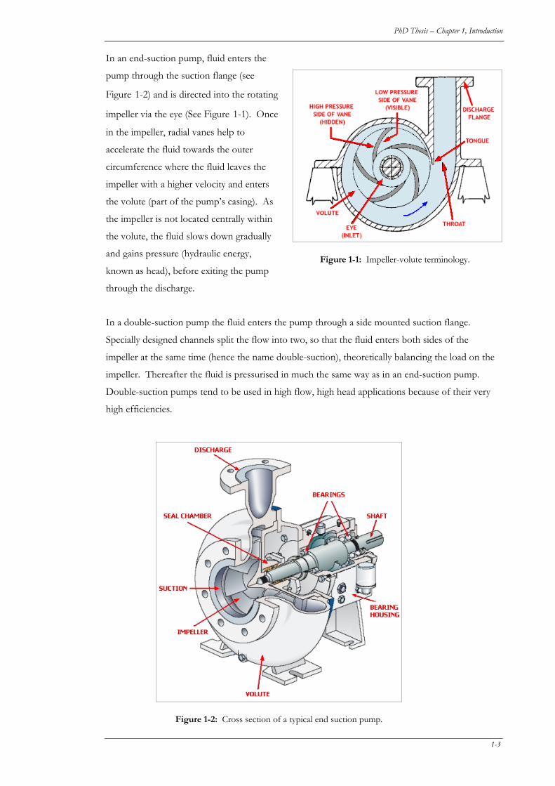
Figure 1-1: Impeller-volute terminology. 1-3
Figure 1-2: Cross section of a typical end suction pump. 1-3
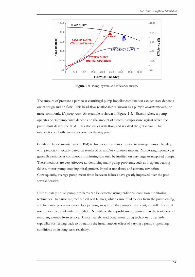
Figure 1-3: Pump, system and efficiency curves. 1-4
Figure 1-4: Onset of adverse conditions caused by operating away from BEP[59]. 1-6
Figure 2-1: Types of AE signals [49]. 2-3
Figure 2-2: Traditional features of an AE signal. 2-3
Figure 2-3: SPM Processing. 2-8
Figure 2-4: Damping effect due to sensor location (from [112]). 2-8
Figure 2-5: Process of extracting a traditional envelope spectrum (from [121]). 2-9
Figure 2-6: PeakVue Processing. 2-10
Figure 2-7: Spike Energy Processing. 2-11
Figure 2-8: Typical Spike Energy signals (from [129]). 2-12
Figure 2-9: SWANTech Processing. 2-13
Figure 2-10: SWE in a centrifugal pump (from [16]). 2-13
Figure 2-11: SEE Processing. 2-14
Figure 2-12: Holroyd Instruments Signal Processing. 2-15
Figure 3-1: PCI2 board block diagram (from [6]). 3-2
Figure 3-2: (A) A signal, (B) its envelope calculated using a Hilbert transform, and (C)
the resulting FFT. 3-5
Figure 4-1: Different amplitude-duration characteristics of AE hits. Data has been
processed by a Swansong II filter but probable EMI noise still remains.
(PUMAnalysis software courtesy of Imes Group Ltd.) 4-3
Figure 4-2: Improved trending is obtained by using the telltale-hit criteria to segregate
bursts from residual changes in the continuous emission level. (A) Shows
the normalised AE feature versus flow determined from the complete
xiii
unfiltered dataset, whilst (B) shows the same normalised feature from a
reduced dataset determined by removing telltale hits. (Vertical lines indicate
90% confidence limits, which increase because the number of hits used to
determine the sample mean reduce. Very few hits remain at normalised
flows between 0.9 and 1.1.) 4-5
Figure 4-3: Effect of frequency and wavelet filters on pump AE signal corrupted by a
100Hz frequency sinusoidal signal and high frequency impulsive noise, latter
emanating from a VFD. (a) Original time signal, (b) FFT, (c) 10kHz –
1000kHz bandpass filtered and (d) 10kHz – 200kHz bandpass filtered. 4-7
Figure 4-4: Effect of averaging on identification of harmonic noise elements hidden
amongst a broadband continuous AE pump signal with (A) 8192 samples
and no averaging, (B) 8192 samples and 8 averages, (C) 8192 samples and
64 averages, and (D) 1024 samples and 64 averages. Sampling rate was
5MHz. 4-8
Figure 4-5: Examples of changes in spectral composition that can be observed in a
typical CWT plot (Morlet wavelet). 4-9
Figure 4-6: Effects on Haar wavelet denoising to 12 levels on two different types of
noise: (A-B) EMI/RFI; (C-D) VFD noise. Due to the impulsive nature of
the noise signals, wavelet denoising is not particularly effective in either case. 4-11
Figure 4-7: Effect of wavelet type on denoised signal. (A) Original waveform, (B)
Denoised with a Haar wavelet, (C) Denoised with a Daubechies 6 wavelet
and (D) Denoised with a Biorthogonal 1-3 wavelet. 4-13
Figure 4-8: Effect of threshold estimating algorithm on low signal to noise ratio signal
(VFD noise): (A) original signal; (B) Using Stein’s unbiased risk estimate,
(C) Using √(2logN), (D) using an alternative algorithm from [45]. 4-14
Figure 4-9: Effect of filtering on the final denoised signal. (A) Original signal, (B) After
denoising by Haar wavelet; (C) 100-1000kHz digital filter applied prior to
denoising by Haar wavelet. 4-15
Figure 4-10: (A) Overall signal RMS levels as they change with flow and (B) separated
continuous and discrete RMS parts as they change with flow. 4-16
Figure 5-1: Physical layout of the implemented DBMAS. 5-6
Figure 5-2: Data flow schematic. 5-7
Figure 5-3: Architecture diagram of AEData. 5-8
xiv
Figure 5-4: AEDMAS layout with main tables, relationships, primary keys (PK) and
foreign keys (FK). Primary, secondary and meta- data tables are designated
by (P), (S) or (M) respectively after the table name. One-to-many
relationships are designated by the symbols 1 and ∝ respectively. 5-8
Figure 5-5: Session data entry form. 5-9
Figure 5-6: Process Files Form extracts information from DTA files and analyses WFS
files. 5-10
Figure 5-7: Process of extracting and/or processing data. 5-12
Figure 5-8: Relating timestamps to test conditions. 5-13
Figure 5-9: Raw AE data and corresponding secondary data obtained for a pump flow
test. 5-15
Figure 6-1: First two longitudinal modes showing normalised phase and group velocities
(latter are shown as dashed lines) for an 8-mm SS316 infinitely long rod
waveguide. Wave speed is normalised with respect to transverse wave
speed, given in equation (6-1). 6-5
Figure 6-2: First four normalised torsional phase velocities for 8-mm diameter, infinitely
long waveguides of different materials. Wave speed is normalised with
respect to transverse wave speed, given in equation 6-3. 6-5
Figure 6-3: (A) Angled 43mm waveguides for MS, Delrin, SS316 and Alumina (Clockwise
from top left). (B) Pointed 43mm waveguides (NC). 6-6
Figure 6-4: Waveguide holder. 6-8
Figure 6-5: Waveguide holder setup (NC). 6-9
Figure 6-6: Time waveforms for flat waveguide samples. Different y-scales are used to
facilitate better appreciation of waveform profiles. Time scales are identical.
(43x8mm samples) 6-11
Figure 6-7: Amplitude for different flat-faced waveguides. 6-11
Figure 6-8: Amplitude versus face angle for all sets of angled samples. 6-12
Figure 6-9: Effect on amplitude by using a pointed waveguide. 6-12
Figure 6-10: Effect of pointed end on rise-times. 6-13
Figure 6-11: Material effects on duration. 6-14
Figure 7-1: Wavelet transforms at different sampling rates (Face-to-face signals). 7-6
xv

Figure 7-2: Difference in resolution between (A) STFT in dBAE and (B) CWT, log scale
(Delrin 51-mm sample). Computing times were 594ms and 15141ms
respectively. 7-6
Figure 7-3: Comparison of results obtained from the custom written programs in (A)
LabVIEW and the (B) AGU-Vallen wavelet tool. LabVIEW parameters:
600 scales, 100 samples per time increment, ~30s processing time. AGU-
Vallen parameters: frequency resolution of 5kHz, 1000 wavelet samples,
~60s processing time. 7-7
Figure 7-4: Amplitude (in dB) - frequency (kHz) spectra of averaged time signals. (Face-
to-face spectrum shown as a shadow on each graph.) 7-9
Figure 7-5: Increasing rod length decreases frequency of resonant peaks. 1st resonant
peak match values given in Table 7-1 (aluminium samples). 7-9
Figure 7-6: Effects of different types of points on the resulting frequency spectrum (43-
mm long, 8-mm diameter aluminium samples). 7-11
Figure 7-7: Effect of points on wavelet spectrograms. 7-11
Figure 7-8: CWT from 43-mm long, 60˚ waveguides (Data sampled at 10 MHz). 7-12
Figure 7-9: Effect of face angles of FFT spectra (43-mm long SS316 samples). 7-13
Figure 7-10:Changes in wavelet spectrograms for changing face angles (30-mm
aluminium samples). 7-13
Figure 7-11: Changes due to different face angles for 30-mm SS316 waveguides do not
correspond with flexural modes (only one shown for clarity). 7-14
Figure 7-12: Wavelet spectrograms with longitudinal mode frequencies. 43 mm x 8 mm
waveguides (Phase modes are shown as dotted lines, group modes as solid
lines). 7-15
Figure 7-13: Mode separation is clearly evident in Delrin waveguides. 7-16
Figure 7-14: Standard amplitude spectrum showing changes in location of 2nd resonance
peak. 7-16
Figure 8-1: (A) Pump, system and efficiency curves. (B) Onset of adverse conditions
caused by operating away from BEP[59]. 8-2
Figure 8-2: Normalised flow curves for two speeds tested 8-5
Figure 8-3: Changes in dynamic pressure with flow. 8-7
Figure 8-4: Discharge Flange Vibrations. 8-7
xvi
Figure 8-5: Results of axial vibration results showing changes in (A) RMS and (B)
Kurtosis. 8-8
Figure 8-6: Energy of hits (y axis) versus time (x axis) versus number of hits (z axis) as
flow is reduced from full flow to low flow at two different speeds for (A)
suction AE and (B) discharge AE. Total energy is superimposed over each
graph. Flows as a ratio of BEP for each test condition are also shown. 8-9
Figure 8-7: Most mean parameters increase at low flows for all signals, whilst only Pump
and Discharge signals increase noticeably at high flows. (Results from test at
997 rpm shown.) 8-10
Figure 8-8: Effect on hit rate (hits per second) by denoising processes: (A) Swansong
filtering and (B) Wavelets. Missing points signify no hits detected at that
condition. Results have not been normalised. Difference in magnitude is
due to (A) being determined from hit data sets and (B) determined from
waveform streaming files collected periodically. 8-10
Figure 8-9: Effect of Swansong II filter on rise time signals. (Discharge AE only
shown, for test at 997 rpm.) 8-11
Figure 8-10: Changes across frequency octave bands for (A) suction AE and (B)
discharge AE. 8-13
Figure 8-11: Changes across wavelet bands for (A) suction AE and (B) discharge AE. 8-13
Figure 8-12: Selected normalised parameters show little sensitivity to changes in speed:
(A) Energy in 2nd Wavelet Band, Suction AE signal and (B) Background
RMS, Discharge AE signal. 8-13
Figure 9-1: (A) Total head and (B) efficiency curves for Pump 2. 9-5
Figure 9-2: (A) Total head and (B) efficiency curves for Pump 4. 9-5
Figure 9-3: (A) Total head and (B) efficiency curves for Pump 5. 9-5
Figure 9-4: (A) Total head and (B) efficiency curves for Pump 6. 9-7
Figure 9-5: (A) Total head and (B) efficiency curves for Pump 7. 9-7
Figure 9-6: (A) Total head and (B) efficiency curves for Pump 8. 9-7
Figure 9-7: Test 8 at 2236rpm. Green line shows raw voltage from flowmeter whilst
black line shows changes in Absolute Energy for PumpAE. At 0.5-0.9BEP,
flow does not remain constant (the control valve was kept in the same
position). 9-8
xvii
Figure 9-8: Hit intensity plots for (A) Pump 6 at 2263rpm, and (B) Pump 7 at 2263rpm.
These show number of hits (z axis) versus PAC Energy (y axis) versus time
(x axis). The superimposed black lines shows time averaged Absolute
Energy. Red lines shows changes in flow (also labelled as %BEP). To
emphasise low energy changes, small numbers of very high-energy events at
low flow are not shown. 9-10
Figure 9-9: Normalised RMS of PumpAE for (A) Group 1 pumps and (B) Group 2
Pumps. 9-11
Figure 9-10: Normalised RMS of PumpAE after wavelet denoising for (A) Group 1
pumps and (B) Group 2 Pumps. 9-11
Figure 9-11: (A) Normalised Peak and (B) Normalised Energy in 12th Wavelet Band for
Group 2 Pumps. 9-11
xviii

LLIISSTT OOFF TTAABBLLEESS
Table 2-1: Comparison of various Stress-wave technologies. 2-22
Table 3-1: Octave and 1/3-octave band frequencies. 3-10
Table 5-1: Characteristics of conventional and data driven processing 5-3
Table 6-1: Approximate acoustic properties of test materials used in theoretical
calculations. 6-6
Table 6-2: Results of rough amplitude calculations. 6-11
Table 7-1: Approximate natural frequencies of first longitudinal mode in cylindrical
rods with differing lengths. 7-2
Table 9-1: Selected data acquisition settings. 9-3
Table 9-2: Sensor data collected from each test. 9-3
xix

NNOOMMEENNCCLLAATTUURREE
AE Acoustic Emission
AET Acoustic Emission Testing
ANN Artificial Neural Network
ANSI American National Standards Institute (governing standards for
chemical process pumps)
API American Petroleum Institute (governing standards for petroleum
process pumps)
AveDBurstDuration Average duration of all bursts detected after denoising
AveDBurstEnergy Average of all energies from bursts detected after wavelet
denoising
AveDBurstPeak Average all the peaks detected in a datafile after wavelet denoising
BA Vibration signals measured on the bearing housing the axial
direction
BgndRMS RMS of the signal components that have been removed by
denoising
BEP Best efficiency point (a flow)
BR Vibration signals measured on the bearing housing in the radial
direction
BV Vibration signals measured on the bearing housing in the vertical
direction
CBM Condition Based Maintenance
CF Crest factor
CM Condition monitoring
COTS Commercial-Off-The-Shelf
DenRMS RMS of the signal after denoising
DEvents Number of events per second after denoising
xx
DPR2 Background RMS / Max DBurst Peak
E Energy
FaceAE AE signals measured on a sensor attached to a waveguide which in
turn is attached to the back of the stationary face and protrudes
through the gland plate
FFT Fast Fourier Transform
GlandAE AE signals measured on the gland plate.
GlandVib Vibration signals measured on the seal stuffing box
H,h Head of the pump, normally in meters, but sometimes in feet
HI Hydraulic Institute
IFD Incipient failure detection
K Kurtosis
MaxDBurstPeak Highest peak detected in a datafile after denoising
MaxDBurstEnergy Maximum energy of bursts detected after denoising
N, n Number of samples
NPSH Net positive suction head
NPSHA Net positive suction head available
NPSHMR Net positive suction head margin ratio
NPSHR Net positive suction head required
P Power
PeakFreq Amplitude of highest peak in FFT
p∞ Static reference pressure of the fluid, or total inlet pressure
pv Equilibrium vapour pressure of the fluid
PumpAE AE signals measured on the pump casing.
PumpVib Vibration signals measured on pump casing
RMS Root mean square
SNR Signal to noise ratio
SE Suction Energy
SflangeAE AE signals measured on the suction nozzle flange of the pump
xxi
sg, SG Specific gravity
SS Specific Speed
SSS or NSS Suction Specific Speed
SpipeVib Vibration signals measured on suction pipe
SuctionAE AE signals measured on the suction pipe.
STD Standard deviation
U∞ Reference speed (usually inlet relative velocity)
UWA University of Western Australia
VFD Variable frequency drive, synonymous with VSD
VSD Variable speed drive
x[n] Array of length n, usually containing the scaled and digitized AE
time signal
x[i] Individual element of the array x[n], where 0<i<n
ρ Fluid density
μ Sample Mean
σ Sample Standard deviation
σ2 Sample Variance
64kPower Normalised power in 63k third octave band
81kPower Normalised power in 81k third octave band
102kPower Normalised power in 101.6k third octave band
128kPower Normalised power in 128k third octave band
161kPower Normalised power in 161.3k third octave band
203kPower Normalised power in 203.2k third octave band
256kPower Normalised power in 256k octave band
322kPower Normalised power in 322.5k octave band
406kPower Normalised power in 406.4k third octave band
512kPower Normalised power in 512k third octave band
645kPower Normalised power in 645k third octave band
xxii

Progress begins when we stop thinking
a problem is difficult
and start believing it is merely complex.
P.J. Kelly
xxiii
1. IINNTTRROODDUUCCTTIIOONN11
1.1 PRELUDE
This project was initiated by the desire to solve a problem. As a maintenance engineer for an oil
refinery, once a month I found myself hopelessly standing by as a centrifugal pump released hot
bitumen onto the plant floor when its mechanical seal failed on start up. Unfortunately, failure did
not occur every time the batch plant started up, and countless investigations had not uncovered any
conclusive evidence of the cause or the operating conditions that preceded the seal’s demise.
Consequently, this PhD began with the intention of developing a technique for monitoring
mechanical seals in service, and to determine what condition indicators preceded failure. Acoustic
emission (AE) was identified as the most appropriate technology for the task.
As the project continued, it became apparent that the following problems had to be solved before a
mechanical seal monitoring system based on AE, could ever be developed for commercial
application.
(a) Commercially available AE systems have been designed for structural monitoring
applications (eg. pressure vessels, cranes etc). AE signals from pumps are very different and
so traditional AE signal processing techniques may need to be supplemented and/or
modified to ensure that they accurately characterise changes in machinery AE signals.
(b) A variety of noise sources, peculiar to machinery monitoring applications, can appear very
similar to acoustic emission sources, and if not identified and removed will, at best, lead to
1-1

PhD Thesis – Chapter 1, Introduction
confusion when interpreting results or at worst, result in a perfectly healthy seal or pump
being removed from service.
(c) As the time of failure is unpredictable, the amount of data that can be collected is
considerable. If the ultimate aim is to detect incipient failure, all of this data needs to be
analysed and scrutinised. To do this manually would be impractical.
(d) When it is impossible to locate a sensor where required (eg. on a seal face), waveguides can
be used. The effect of waveguide shape and material composition needs to be understood so
that signals can be interpreted correctly.
(e) Acoustic emissions collected from the seal are strongly influenced by the hydraulic
conditions within the pump. Therefore, to be able to differentiate between an incipient seal
failure and an unfavourable hydraulic condition, the latter must be identified. To do this, the
pump’s individual acoustic emission signature needs to be characterised.
(f) Mechanical seal failures need to be initiated in a controlled but realistic environment so that a
statistically significant amount of AE data can be collected, and the precursors to failure
identified.
(g) Electronics for collecting and analysing AE data are currently too expensive and
cumbersome. Physically smaller, more robust and cost effective alternatives are required for
continuous AE monitoring applications.
This thesis then became a process of investigating and overcoming each of these obstacles in turn.
Although sufficient time was not available to develop a seal-monitoring system, as solutions to last
two challenges are still proving elusive, the ultimate goal is now much closer to being realised.
1.2 BACKGROUND
Centrifugal pumps are the most prevalent electrically powered, rotating machine used today. Of
these, most are single-stage with end-suctions as shown in Figure 1-2.
A centrifugal pump moves fluid from one point to another by converting mechanical energy into
hydraulic energy through centrifugal action. The hydraulic energy is referred to as head and is
measured in meters.
1-2
PhD Thesis – Chapter 1, Introduction
In an end-suction pump, fluid enters the
pump through the suction flange (see
Figure 1-2
) and is directed into the rotating
impeller via the eye (See Figure 1-1). Once
in the impeller, radial vanes help to
accelerate the fluid towards the outer
circumference where the fluid leaves the
impeller with a higher velocity and enters
the volute (part of the pump’s casing). As
the impeller is not located centrally within
the volute, the fluid slows down gradually
and gains pressure (hydraulic energy,
known as head), before exiting the pump
through the discharge.
Figure 1-1: Impeller-volute terminology.
In a double-suction pump the fluid enters the pump through a side mounted suction flange.
Specially designed channels split the flow into two, so that the fluid enters both sides of the
impeller at the same time (hence the name double-suction), theoretically balancing the load on the
impeller. Thereafter the fluid is pressurised in much the same way as in an end-suction pump.
Double-suction pumps tend to be used in high flow, high head applications because of their very
high efficiencies.
Figure 1-2: Cross section of a typical end suction pump.
1-3
PhD Thesis – Chapter 1, Introduction
Figure 1-3: Pump, system and efficiency curves.
The amount of pressure a particular centrifugal pump-impeller combination can generate depends
on its design and on flow. This head-flow relationship is known as a pump’s characteristic curve, or
more commonly, it’s pump curve. An example is shown in Figure 1-3. Exactly where a pump
operates on its pump curve depends on the amount of system backpressure against which the
pump must deliver the fluid. This also varies with flow, and is called the system curve. The
intersection of both curves is known as the duty point.
Condition based maintenance (CBM) techniques are commonly used to manage pump reliability,
with prediction typically based on results of oil and/or vibration analysis. Monitoring frequency is
generally periodic as continuous monitoring can only be justified on very large or unspared pumps.
These methods are very effective at identifying many pump problems, such as incipient bearing
failure, motor-pump coupling misalignment, impeller unbalance and extreme cavitation.
Consequently, average pump mean times between failures have greatly improved over the past
several decades.
Unfortunately not all pump problems can be detected using traditional condition monitoring
techniques. In particular, mechanical seal failures, which cause fluid to leak from the pump casing,
and hydraulic problems caused by operating away from the pump’s duty point, are still difficult, if
not impossible, to identify or predict. Nowadays, these problems are more often the root cause of
removing pumps from service. Unfortunately, traditional monitoring techniques offer little
capability for feeding back to operators the instantaneous effect of varying a pump’s operating
conditions on its long-term reliability.
1-4
PhD Thesis – Chapter 1, Introduction
Efficiency of the mechanical-hydraulic energy conversion varies with flow, as shown in Figure 1-3.
Maximum input energy is converted into increased head at the Best Efficiency Point (BEP). In
well-designed systems, the duty point is close to BEP. However, due to system resistance changes,
poor design or control valve throttling, pumps are often forced to operate far away from their BEP.
This causes hydraulic, thermal and mechanical losses to increase, in addition to a number of more
serious adverse effects, as shown in Figure 1-4.
No published data has been obtained regarding the cost of suboptimal pump operation and/or
failure in Australia, however correlations can be made with results of reviews undertaken in other
countries. According to a 2001 report by the AEAT [33], centrifugal pumps in the European
Union use approximately 117TWH of electricity per annum, which is 10% of all electricity
consumed by industry and commerce in the EU, and account for 58MT of CO2 emissions (1998
figures). The report states that the “largest energy savings are to be made through the better design
and control of pump systems” and “efficiency may fall off fast as operation moves from the Best
Efficiency Point”. It also recognizes that “on average, pumps operate at flows below their best-
efficiency flow”. Although the report does not quantify how inefficiently pumps are being
operated, a similar study in Finland claims that of the 1690 centrifugal pumps reviewed in detail,
average efficiency was less than 40%[56]. Typical BEP values range between 55% and 80%; thus it
can be concluded that most pumps studied in the Finnish review were not operating close to their
BEP value.
1-5
PhD Thesis – Chapter 1, Introduction
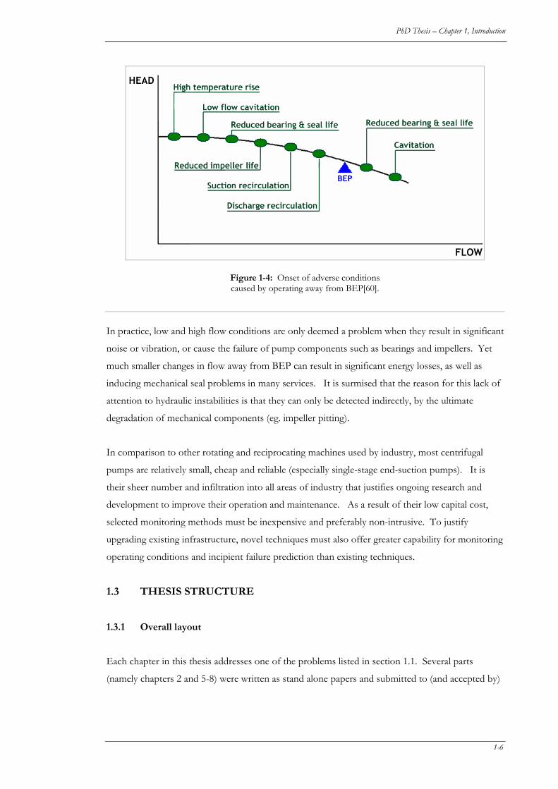
Figure 1-4: Onset of adverse conditions caused by operating away from BEP[60].
In practice, low and high flow conditions are only deemed a problem when they result in significant
noise or vibration, or cause the failure of pump components such as bearings and impellers. Yet
much smaller changes in flow away from BEP can result in significant energy losses, as well as
inducing mechanical seal problems in many services. It is surmised that the reason for this lack of
attention to hydraulic instabilities is that they can only be detected indirectly, by the ultimate
degradation of mechanical components (eg. impeller pitting).
In comparison to other rotating and reciprocating machines used by industry, most centrifugal
pumps are relatively small, cheap and reliable (especially single-stage end-suction pumps). It is
their sheer number and infiltration into all areas of industry that justifies ongoing research and
development to improve their operation and maintenance. As a result of their low capital cost,
selected monitoring methods must be inexpensive and preferably non-intrusive. To justify
upgrading existing infrastructure, novel techniques must also offer greater capability for monitoring
operating conditions and incipient failure prediction than existing techniques.
1.3 THESIS STRUCTURE
1.3.1 Overall layout
Each chapter in this thesis addresses one of the problems listed in section 1.1. Several parts
(namely chapters 2 and 5-8) were written as stand alone papers and submitted to (and accepted by)
1-6
PhD Thesis – Chapter 1, Introduction
referred journals or conferences. The associated publication reference is given at the beginning of
each chapter, followed by its aim.
A literature review covering the body of work relevant to a particular problem statement is
contained within each chapter. As a result, if papers were to be presented herein as they were
published, considerable repetition would ensue. Therefore, for brevity, review sections of papers
containing considerable repetition have been replaced with appropriate linking statements.
Conversely, for the sake of relevance and continuity, some additional content has been added
subsequent to a paper’s publication. This is designated with a ‘NC’ (New Content) after the
relevant section header and predominantly relates to chapter aims and postscripts. Other than
minor linguistic improvements, no content has been removed or altered.
Several papers were co-authored. Consequently, the extent to which these co-authors contributed
to each body of work is detailed below. Furthermore, a set of initials (eg. MH or PK) in a section’s
header designates it as having been written, or the underlying work performed by, the respective
co-author. In all cases, Professors Michael Norton or Jie Pan offered general supervisory guidance
and oversight.
1.3.2 Chapter topics
Most current state of the art systems for detecting incipient machinery faults have been undertaken
by corporately, or privately funded researchers who tend to commercialise, rather than publish their
findings. Consequently, chapter 2 contains a review of systems available on the market (in 2003) by
analysing their underlying patents and research findings. It also suggests why the maintenance
community has not readily accepted AE technology, and suggests how this might be rectified in the
future. Published at a maintenance conference in 2003, this paper helps maintenance professionals
determine how best to interpret and compare results obtained with one system against results
collected with another. It also provided the basis for development of in-house electronics used in
this research project.
Chapter 3 outlines signal processing theory relevant to subsequent chapters. Basic statistical
analysis, wavelet and octave band analysis are discussed. These techniques are not usually applied
to acoustic emission testing, so their appropriate application needs to be carefully considered.
Equations, developed by the author, for computing statistics of long arrays from shorter subsets of
the array are also presented, facilitating faster and more efficient processing of long waveforms.
1-7
PhD Thesis – Chapter 1, Introduction
As acoustic emission signals are very small, analysis is complicated by the ingress of noise. Chapter
4 describes various techniques that were applied to separate noise from acoustic emission activity of
interest, thus improving the likelihood of detecting trends relating to incipient faults or failure
conditions. These techniques are either not usually applied to the AE signals from machinery or
their application to AE monitoring of machinery has not been detailed before. Examples of how
these techniques were applied to AE data collected by the author from centrifugal pumps are given.
Condition monitoring creates huge volumes of AE data that cannot be processed manually. To
overcome this problem, a relational database was developed with the help of Mr Paul Kelly, an IT
systems architect, for analysing and managing tens of gigabytes of AE data collected during the
course of pump experiments. This system is described in Chapter 5. In the work described
therein, Mr Kelly setup the hardware, provided advice on the overall system architecture and wrote
many of the advanced visual basic and SQL routines used by the database. Conversely, the author
defined the user requirements, designed most of the user interfaces, wrote many of the simpler
code modules and queries to extract data and developed all advanced signal processing routines.
This system allowed the author to process over 250GB of AE data collected during various stages
of this research project.
Waveguides are often necessary to provide simpler transmission paths from otherwise inaccessible
components (eg. mechanical seals), or to separate delicate sensors from hot machinery and/or
strong magnetic fields. However, it is hypothesised that they also complicate analysis significantly.
To clarify these interactions, Chapters 6 and 7 contain two published papers that verify, for the first
time, the temporal and frequency changes to AE simulated signals as they pass through short, solid,
cylindrical rods of varying materials, diameters and face angles. Basic waveguide theory is also
summarised, demonstrating the author’s familiarity with relevant acoustic emission wave theory.
Chapter 8 presents a case study on how AE monitoring, using the signal processing and data
management techniques described in the preceding chapters, can be used to successfully detect
changes in flow within a double-suction pump. It is based on a Comadem conference paper that
was written with Dr Melinda Hodkiewicz, who analysed vibration and dynamic pressure signals
against which AE trends are compared. This is the first time such results have been presented.
The cumulative results of flow tests on a number of small end-suction centrifugal pumps are
presented in Chapter 9. This facilitates analysis of the similarities and differences in AE behaviour
between pumps, which again has not been reported previously. The sensitivity of AE to the testing
process is also discussed and suggestions are offered to improve the accuracy of AE results
obtained from pump experiments.
1-8

PhD Thesis – Chapter 1, Introduction
Finally, Chapter 10 discusses the overall conclusions from this work and how the preceding
chapters contribute to the overcoming the challenges identified in Section 1-1. Numbered
references from all chapters are listed alphabetically in Chapter 11.
1-9
2. R
2-1
REEVVIIEEWW OOFF AAEE
TTEECCHHNNOOLLOOGGYY 22
Sikorska, J. and Norton, M.P.,
Proceedings of ICOMS 2003,
Perth Australia, Paper 011 pp.1-13
The aims of this chapter are to:
(a) Review signal processing techniques used for the detection of faults in rotating equipment
by analysing published works and relevant patents; and
(b) Identify problems that would need to be overcome for AE monitoring tools to be more
widely accepted by the maintenance community.
Publication Abstract
Acoustic emission (AE) has been used as an NDT technique for incipient fault detection since the
1960’s, but it is not widely applied to machine condition monitoring. Yet research indicates that
AE can be a very powerful tool for detecting impulsive faults, such as wear, lubrication problems
and impacts in bearings, gears and mechanical seals. Various proprietary “black box” instruments,
collectively referred to as stress wave analysis tools, are being offered by vibration equipment
manufacturers. However their operating principles and relationship to acoustic emission is unclear.
This may be a contributing factor to the restricted adoption of AE by the condition monitoring
community. To remove some of these barriers, this paper explains how these instruments measure
and characterise acoustic emissions generated by faults within a machine. It also discusses how
with a better understanding of the underlying principles by users, and a few minor technological
improvements by manufacturers, acoustic emission can become a powerful and affordable incipient
failure detection tool for many rotating equipment components.

PhD Thesis – Chapter 2, Review of AE Systems
2.1 INTRODUCTION
Acoustic emissions (AE) are high frequency elastic waves generated by the release of energy from
micro- and macroscopic defects within a material. They are also known as stress waves and are
generated in discrete packets, the amplitude, direction and polarization of which depend on the
material’s crystalline structure [12]. In general, the amount of elastic energy released is proportional
to the volume of the sample, the speed of deformation and the amount of micro-damage created
[25].
Common sources of stress that can cause AE generation include material fracture, crack nucleation
and growth, phase changes, or variations in external conditions that produce a static imbalance or
phase instability. Consequently, it has been used as a non-destructive monitoring technique for
over thirty years. Condition monitoring of machinery is a more recent application of this
technology, however its extension to the detection of defects in bearings, gearboxes and other
structural components is obvious. After all, most machinery problems result from material
degradation (be it wear, fatigue or overstressing) or extraneous fluid-structure interactions (e.g.
cavitation). These have all been shown to generate acoustic emissions and a brief overview of
relevant research will be given in the following section. Though many of these failure modes can
be detected by vibration monitoring, it has determined that acoustic emissions generated by these
faults precede detectable vibrations [120], particularly in low speed equipment.
A question therefore needs to be asked: “why is AE not being more widely used for detecting
incipient machinery faults?” The answer is that in fact it is, albeit under a variety of different names
and in a rather limited capacity. Unfortunately, not only is it difficult or impossible to compare the
output of one system against another, very few objective comparisons have been undertaken.
Therefore, users have no option but to believe a manufacturer’s sales literature on why their
particular technology variant is superior to any other. Furthermore, many of these systems give
their output in the form of one or more ‘magic numbers’, yet supply little or no information on
how these are derived. It is therefore not surprising that AE is viewed with a degree of scepticism
by the condition monitoring community.
This paper will address some of the confusion surrounding the use of AE for diagnosing incipient
machinery faults. After summarizing initial research in this area, the main commercially available
technologies will be explained. It is important to be aware that these explanations are the authors’
interpretations of available literature and original manufacturers’ patents. However, only the
manufacturers could clarify this any further and then only for their product. Consequently, the
authors believe that by presenting these systems collectively, users can better appreciate the
potential and limitations of available acoustic emission technology.
2-2
PhD Thesis – Chapter 2, Review of AE Systems
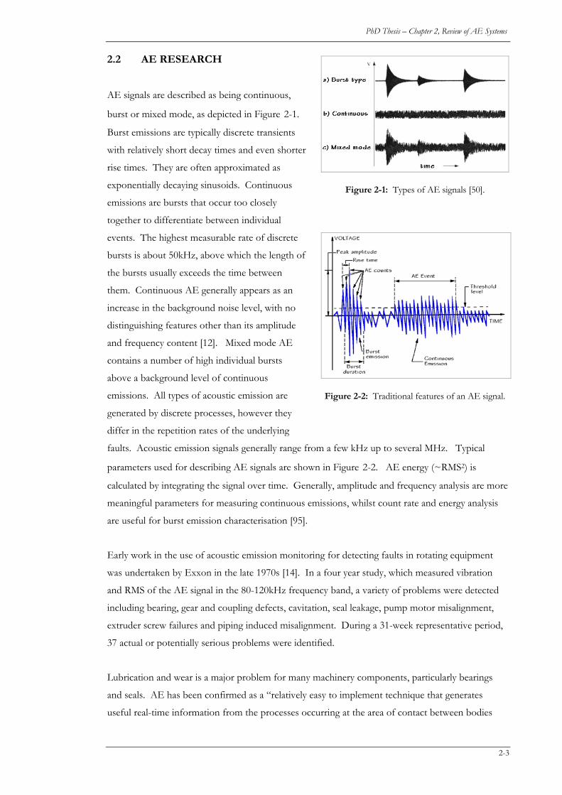
2.2 AE RESEARCH
AE signals are described as being continuous,
burst or mixed mode, as depicted in Figure 2-1.
Burst emissions are typically discrete transients
with relatively short decay times and even shorter
rise times. They are often approximated as
exponentially decaying sinusoids. Continuous
emissions are bursts that occur too closely
together to differentiate between individual
events. The highest measurable rate of discrete
bursts is about 50kHz, above which the length of
the bursts usually exceeds the time between
them. Continuous AE generally appears as an
increase in the background noise level, with no
distinguishing features other than its amplitude
and frequency content [12]. Mixed mode AE
contains a number of high individual bursts
above a background level of continuous
emissions. All types of acoustic emission are
generated by discrete processes, however they
differ in the repetition rates of the underlying
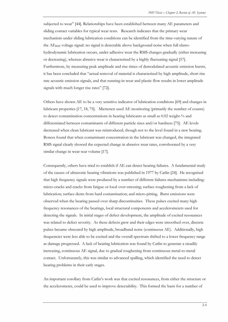
faults. Acoustic emission signals generally range from a few kHz up to several MHz. Typical
parameters used for describing AE signals are shown in Figure 2-2
Figure 2-1: Types of AE signals [50].
Figure 2-2: Traditional features of an AE signal.
. AE energy (~RMS2) is
calculated by integrating the signal over time. Generally, amplitude and frequency analysis are more
meaningful parameters for measuring continuous emissions, whilst count rate and energy analysis
are useful for burst emission characterisation [95].
Early work in the use of acoustic emission monitoring for detecting faults in rotating equipment
was undertaken by Exxon in the late 1970s [14]. In a four year study, which measured vibration
and RMS of the AE signal in the 80-120kHz frequency band, a variety of problems were detected
including bearing, gear and coupling defects, cavitation, seal leakage, pump motor misalignment,
extruder screw failures and piping induced misalignment. During a 31-week representative period,
37 actual or potentially serious problems were identified.
Lubrication and wear is a major problem for many machinery components, particularly bearings
and seals. AE has been confirmed as a “relatively easy to implement technique that generates
useful real-time information from the processes occurring at the area of contact between bodies
2-3
PhD Thesis – Chapter 2, Review of AE Systems
subjected to wear” [44]. Relationships have been established between many AE parameters and
sliding contact variables for typical wear tests. Research indicates that the primary wear
mechanism under sliding lubrication conditions can be identified from the time-varying nature of
the AERMS voltage signal: no signal is detectable above background noise when full elasto-
hydrodynamic lubrication occurs, under adhesive wear the RMS changes gradually (either increasing
or decreasing), whereas abrasive wear is characterised by a highly fluctuating signal [57].
Furthermore, by measuring peak amplitude and rise times of demodulated acoustic emission bursts,
it has been concluded that “actual removal of material is characterised by high amplitude, short rise
rate acoustic emission signals, and that running-in wear and plastic flow results in lower amplitude
signals with much longer rise rates” [72].
Others have shown AE to be a very sensitive indicator of lubrication conditions [69] and changes in
lubricant properties [17, 18, 75]. Miettenen used AE monitoring (primarily the number of counts)
to detect contamination concentrations in bearing lubricants as small as 0.02 weight-% and
differentiated between contaminants of different particle sizes and/or hardness [75]. AE levels
decreased when clean lubricant was reintroduced, though not to the level found in a new bearing.
Boness found that when contaminant concentration in the lubricant was changed, the integrated
RMS signal clearly showed the expected change in abrasive wear rates, corroborated by a very
similar change in wear scar volume [17].
Consequently, others have tried to establish if AE can detect bearing failures. A fundamental study
of the causes of ultrasonic bearing vibrations was published in 1977 by Catlin [24]. He recognised
that high frequency signals were produced by a number of different failures mechanisms including:
micro-cracks and cracks from fatigue or local over-stressing; surface roughening from a lack of
lubrication; surface dents from hard contamination; and micro-pitting. Burst emissions were
observed when the bearing passed over sharp discontinuities. These pulses excited many high
frequency resonances of the bearings, local structural components and accelerometers used for
detecting the signals. In initial stages of defect development, the amplitude of excited resonances
was related to defect severity. As these defects grew and their edges were smoothed over, discrete
pulses became obscured by high amplitude, broadband noise (continuous AE). Additionally, high
frequencies were less able to be excited and the overall spectrum shifted to a lower frequency range
as damage progressed. A lack of bearing lubrication was found by Catlin to generate a steadily
increasing, continuous AE signal, due to gradual roughening from continuous metal-to-metal
contact. Unfortunately, this was similar to advanced spalling, which identified the need to detect
bearing problems in their early stages.
An important corollary from Catlin’s work was that excited resonances, from either the structure or
the accelerometer, could be used to improve detectability. This formed the basis for a number of
2-4
PhD Thesis – Chapter 2, Review of AE Systems
patented systems that will be discussed below. Good reviews of bearing vibration monitoring by
such techniques are given in [73].
In the 1980’s and 1990’s a diagnostic algorithm to identify a variety of faults in journal bearings was
developed [102, 103]. They separated the signals into burst and continuous emissions and
characterised frequency information as either wideband or narrowband, and either tuned to the
rotating speed or untuned. Depending on these classifications, the authors were able to correctly
diagnose rubbing, metal wipe, and bearing tilt, as well as rotor cracks, fatigue cracks and radial plane
damage. Although metal wipe could be monitored with conventional AE techniques (clear patterns
could be identified in the time signal and envelope), an envelope spectrum was required to diagnose
running and bearing tilt. A similar model was developed for incipient failures in rotary air
conditioning compressors [104] where the difference between abrasive wear and vane butting were
identified. Turbine rotor rubbing has also been detected [54] at bearing housings up to 2m away
[71].
In addition to frequency analysis of AE signals (or demodulated AE) a variety of other advanced
techniques have been used to better identify bearing defects. These include autoregressive
coefficients [55], Point Process Spectral Averaging [59], adaptive noise techniques [121] and pattern
recognition analysis [65].
Slow speed equipment can be problematic for vibration analysts due to the limitations imposed by
instrumentation (at low frequencies), low energies of fault frequencies and the use of
accelerometers rather than displacement probes for routine measurement. In these applications,
research has shown that AE can detect simulated faults in rolling element bearings rotating between
1 and 100rpm [54, 55, 99], although there does seem to be some disagreement as to the required
size of the fault before detection is guaranteed, particularly for inner race defects where
transmission paths are complex [54, 55, 123]. In Tandon and Nakra’s work, AE counts were also
shown to increase with load [123]. Others have also identified unbalance in low speed equipment
by demodulated resonance analysis [21].
AE has also been shown to be capable of detecting a variety of fluid borne problems in machinery
[53]. In 1977, Derakshan et al showed that “acoustic emissions” are generated during bubble
generation and collapse and determined that cavitation intensity in a hydroturbine was proportional
to the RMS of the acoustic emission signal [29]. Finley also observed that cavitation in machinery
was easily detectable as “high amplitude excursions in the RMS”[34]. More recently, Neill et al
were also able to detect cavitation in centrifugal pumps as well differentiating it from recirculation
[80, 81]. Board has also shown that changes in pump flow conditions (cavitation, recirculation and
best efficiency) can be detected by stress wave energy levels [16] (See Figure 2-10).
2-5
PhD Thesis – Chapter 2, Review of AE Systems
Failure of mechanical seals has also been detected by acoustic emission analysis. A continuous
monitoring system was implemented in a Japanese refinery that measured AERMS and it was found
that one of four patterns was observed in a seal’s AE trends prior to failure [61]. The authors
concluded that instability in the AE signal corresponded to instability in the lubricating film and
that an estimation of wear speed and wear amount is possible by monitoring seal emissions.
Similar results were reported by others who identified leakage, dry running and cavitation in the seal
gap by measuring acoustic emissions (with RMS) [76] and determined that acoustic emission
variations coincided with torque and temperature variations during sliding wear [68].
2.3 EXISTING TECHNOLOGY
2.3.1 Shock pulse – SPM Instruments
Shock pulse was first developed and patented in Sweden in the early 1970’s by SPM Instruments
[112, 114]. It involves measuring and analyzing high frequency shock waves that are generated by a
rotating bearing and detected by a piezoelectric accelerometer resonant at 32kHz. SPM’s initial
research found that shock pulse amplitude is based on rolling velocity, oil film thickness and the
mechanical condition of the mating faces. They also discovered that in an undamaged bearing,
although the maximum level of these stress waves depended on the thickness of the lubricant, the
ratio between peak values and the baseline “noise” level did not change. Surface damage however,
affected this ratio dramatically [78]. Later work determined that amplitude was also determined by
sensor location with respect to the load zone [113].
SPM then undertook a vast amount of testing on control bearings to determine relationships
between:
• Lubricant film parameter, Λ, and shock pulse value in decibels (dBBsv)
• The difference in dBsv under lubricated and dry running conditions
• Lubricant film thickness and dBsv for a fixed sliding velocity
• The baseline dBsv (i.e. in a good bearing) for various bearing types and sliding velocities
Over 9943 sets of real-time data from a variety of bearing types, sizes, manufacturers, lubricants
and loads were collected.
To ascertain the condition of an operating bearing, shock pulse readings can be taken from
operating bearings and the values compared against this known data. Additional processing then
translates this diagnosis into simple parameters that can be trended.
2-6
PhD Thesis – Chapter 2, Review of AE Systems
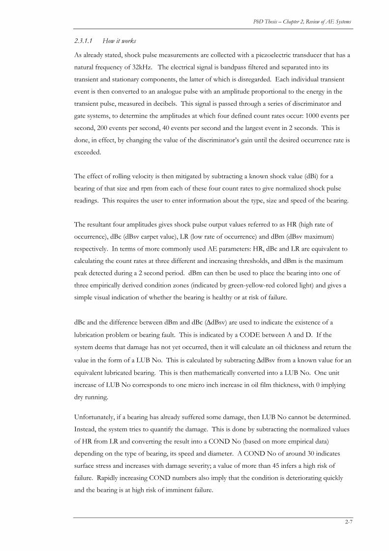
2.3.1.1 How it works
As already stated, shock pulse measurements are collected with a piezoelectric transducer that has a
natural frequency of 32kHz. The electrical signal is bandpass filtered and separated into its
transient and stationary components, the latter of which is disregarded. Each individual transient
event is then converted to an analogue pulse with an amplitude proportional to the energy in the
transient pulse, measured in decibels. This signal is passed through a series of discriminator and
gate systems, to determine the amplitudes at which four defined count rates occur: 1000 events per
second, 200 events per second, 40 events per second and the largest event in 2 seconds. This is
done, in effect, by changing the value of the discriminator’s gain until the desired occurrence rate is
exceeded.
The effect of rolling velocity is then mitigated by subtracting a known shock value (dBi) for a
bearing of that size and rpm from each of these four count rates to give normalized shock pulse
readings. This requires the user to enter information about the type, size and speed of the bearing.
The resultant four amplitudes gives shock pulse output values referred to as HR (high rate of
occurrence), dBc (dBsv carpet value), LR (low rate of occurrence) and dBm (dBsv maximum)
respectively. In terms of more commonly used AE parameters: HR, dBc and LR are equivalent to
calculating the count rates at three different and increasing thresholds, and dBm is the maximum
peak detected during a 2 second period. dBm can then be used to place the bearing into one of
three empirically derived condition zones (indicated by green-yellow-red colored light) and gives a
simple visual indication of whether the bearing is healthy or at risk of failure.
dBc and the difference between dBm and dBc (ΔdBsv) are used to indicate the existence of a
lubrication problem or bearing fault. This is indicated by a CODE between A and D. If the
system deems that damage has not yet occurred, then it will calculate an oil thickness and return the
value in the form of a LUB No. This is calculated by subtracting ΔdBsv from a known value for an
equivalent lubricated bearing. This is then mathematically converted into a LUB No. One unit
increase of LUB No corresponds to one micro inch increase in oil film thickness, with 0 implying
dry running.
Unfortunately, if a bearing has already suffered some damage, then LUB No cannot be determined.
Instead, the system tries to quantify the damage. This is done by subtracting the normalized values
of HR from LR and converting the result into a COND No (based on more empirical data)
depending on the type of bearing, its speed and diameter. A COND No of around 30 indicates
surface stress and increases with damage severity; a value of more than 45 infers a high risk of
failure. Rapidly increasing COND numbers also imply that the condition is deteriorating quickly
and the bearing is at high risk of imminent failure.
2-7
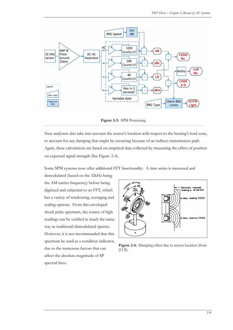
PhD Thesis – Chapter 2, Review of AE Systems
Figure 2-3: SPM Processing.
New analysers also take into account the sensor’s location with respect to the bearing’s load zone,
to account for any damping that might be occurring because of an indirect transmission path.
Again, these calculations are based on empirical data collected by measuring the effect of position
on expected signal strength (See Figure 2-4).
Some SPM systems now offer additional FFT functionality. A time series is measured and
demodulated (based on the 32kHz being
the AM carrier frequency) before being
digitized and subjected to an FFT, which
has a variety of windowing, averaging and
scaling options. From this enveloped
shock pulse spectrum, the source of high
readings can be verified in much the same
way as traditional demodulated spectra.
However, it is not recommended that this
spectrum be used as a condition indicator,
due to the numerous factors that can
affect the absolute magnitude of SP
spectral lines.
Figure 2-4: Damping effect due to sensor location (from [113]).
2-8

PhD Thesis – Chapter 2, Review of AE Systems
2.3.2 CSI PeakVue
CSI’s PeakVueTM technology uses an ordinary accelerometer to measure the stress waves. Based on
research undertaken by Robinson et al [99] a patent was lodged in 1998 [100]. Subsequently, CSI
(now Emerson Process Management) manufactured this system, which measures peak values of the
accelerometer signal and can determine:
• Amplitude of individual stress wave events
• Approximate duration of individual stress wave events
• Rate of stress wave events
Processing can be undertaken by analog or digital systems to display time and frequency
information. PeakVue is a standard feature of most CSI portable analysers.
PeakVue was developed to overcome the traditional deficiencies of demodulation: namely
difficulties in determining an appropriate bandwidth and reduced amplitude accuracy.
2.3.2.1 How it works
This system is best described by comparing it to a standard enveloping system, commonly used for
identifying bearing faults. Both approaches are based on the premise that impulsive events (eg.
bearing faults, gear tooth interactions) cause regular excitation of natural frequencies in either the
structure or sensor, resulting in a signal where the fault frequency is modulating a higher frequency
carrier. Demodulation (also known as enveloping) involves passing this signal through a series of
filters and rectifying it prior to analysis or digitisation to isolate the fault from its carrier.
2.3.2.2 Envelope Analysis
The process of demodulation is shown in Figure 2-5. Firstly, a high pass (HP) filter removes low
frequency components such as rotating speed and its harmonics from the signal, whilst leaving the
higher forcing frequencies of interest and/or their harmonics. The signal is then rectified before
Figure 2-5: Process of extracting a traditional envelope spectrum (from [122]).
2-9
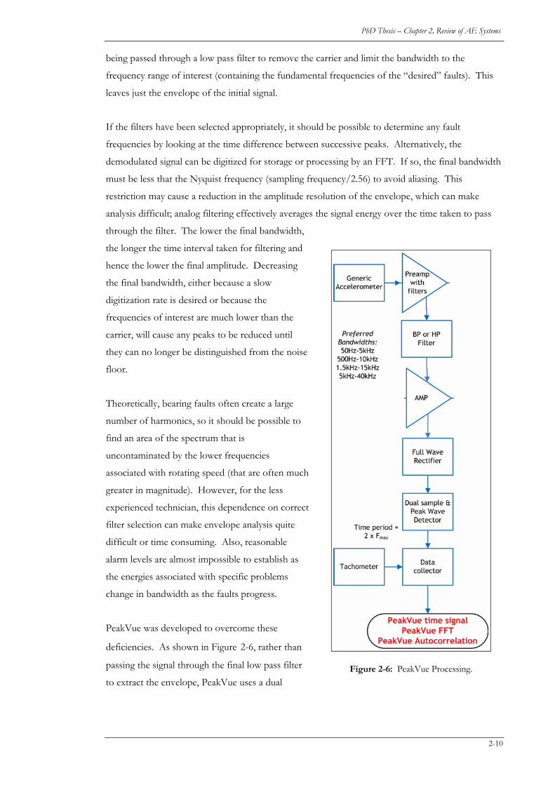
PhD Thesis – Chapter 2, Review of AE Systems
being passed through a low pass filter to remove the carrier and limit the bandwidth to the
frequency range of interest (containing the fundamental frequencies of the “desired” faults). This
leaves just the envelope of the initial signal.
If the filters have been selected appropriately, it should be possible to determine any fault
frequencies by looking at the time difference between successive peaks. Alternatively, the
demodulated signal can be digitized for storage or processing by an FFT. If so, the final bandwidth
must be less that the Nyquist frequency (sampling frequency/2.56) to avoid aliasing. This
restriction may cause a reduction in the amplitude resolution of the envelope, which can make
analysis difficult; analog filtering effectively averages the signal energy over the time taken to pass
through the filter. The lower the final bandwidth,
the longer the time interval taken for filtering and
hence the lower the final amplitude. Decreasing
the final bandwidth, either because a slow
digitization rate is desired or because the
frequencies of interest are much lower than the
carrier, will cause any peaks to be reduced until
they can no longer be distinguished from the noise
floor.
Theoretically, bearing faults often create a large
number of harmonics, so it should be possible to
find an area of the spectrum that is
uncontaminated by the lower frequencies
associated with rotating speed (that are often much
greater in magnitude). However, for the less
experienced technician, this dependence on correct
filter selection can make envelope analysis quite
difficult or time consuming. Also, reasonable
alarm levels are almost impossible to establish as
the energies associated with specific problems
change in bandwidth as the faults progress.
PeakVue was developed to overcome these
deficiencies. As shown in Figure 2-6, rather than
passing the signal through the final low pass filter
to extract the envelope, PeakVue uses a dual Figure 2-6: PeakVue Processing.
2-10
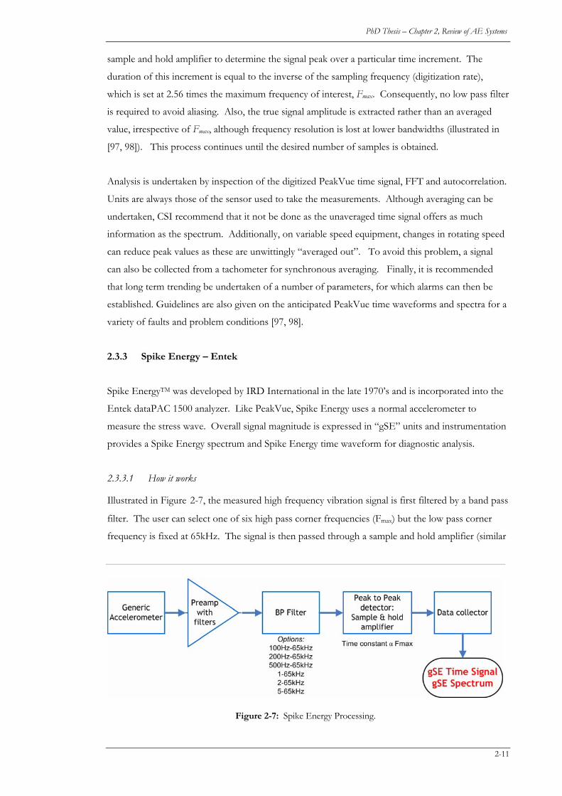
PhD Thesis – Chapter 2, Review of AE Systems
sample and hold amplifier to determine the signal peak over a particular time increment. The
duration of this increment is equal to the inverse of the sampling frequency (digitization rate),
which is set at 2.56 times the maximum frequency of interest, Fmax. Consequently, no low pass filter
is required to avoid aliasing. Also, the true signal amplitude is extracted rather than an averaged
value, irrespective of Fmax, although frequency resolution is lost at lower bandwidths (illustrated in
[97, 98]). This process continues until the desired number of samples is obtained.
Analysis is undertaken by inspection of the digitized PeakVue time signal, FFT and autocorrelation.
Units are always those of the sensor used to take the measurements. Although averaging can be
undertaken, CSI recommend that it not be done as the unaveraged time signal offers as much
information as the spectrum. Additionally, on variable speed equipment, changes in rotating speed
can reduce peak values as these are unwittingly “averaged out”. To avoid this problem, a signal
can also be collected from a tachometer for synchronous averaging. Finally, it is recommended
that long term trending be undertaken of a number of parameters, for which alarms can then be
established. Guidelines are also given on the anticipated PeakVue time waveforms and spectra for a
variety of faults and problem conditions [97, 98].
2.3.3 Spike Energy – Entek
Spike EnergyTM was developed by IRD International in the late 1970’s and is incorporated into the
Entek dataPAC 1500 analyzer. Like PeakVue, Spike Energy uses a normal accelerometer to
measure the stress wave. Overall signal magnitude is expressed in “gSE” units and instrumentation
provides a Spike Energy spectrum and Spike Energy time waveform for diagnostic analysis.
2.3.3.1 How it works
Illustrated in Figure 2-7, the measured high frequency vibration signal is first filtered by a band pass
filter. The user can select one of six high pass corner frequencies (Fmax) but the low pass corner
frequency is fixed at 65kHz. The signal is then passed through a sample and hold amplifier (similar
Figure 2-7: Spike Energy Processing.
2-11
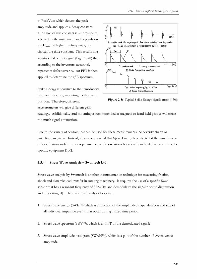
PhD Thesis – Chapter 2, Review of AE Systems
to PeakVue) which detects the peak
amplitude and applies a decay constant.
The value of this constant is automatically
selected by the instrument and depends on
the Fmax, the higher the frequency, the
shorter the time constant. This results in a
saw-toothed output signal (Figure 2-8) that,
according to the inventors, accurately
represents defect severity. An FFT is then
applied to determine the gSE spectrum.
Spike Energy is sensitive to the transducer’s
resonant response, mounting method and
position. Therefore, different
accelerometers will give different gSE
readings. Additionally, stud mounting is recommended as magnets or hand held probes will cause
too much signal attenuation.
Figure 2-8: Typical Spike Energy signals (from [130]).
Due to the variety of sensors that can be used for these measurements, no severity charts or
guidelines are given. Instead, it is recommended that Spike Energy be collected at the same time as
other vibration and/or process parameters, and correlations between them be derived over time for
specific equipment [130].
2.3.4 Stress Wave Analysis – Swantech Ltd
Stress wave analysis by Swantech is another instrumentation technique for measuring friction,
shock and dynamic load transfer in rotating machinery. It requires the use of a specific Swan
sensor that has a resonant frequency of 38.5kHz, and demodulates the signal prior to digitization
and processing [4]. The three main analysis tools are:
1. Stress wave energy (SWETM) which is a function of the amplitude, shape, duration and rate of
all individual impulsive events that occur during a fixed time period;
2. Stress wave spectrum (SWSTM), which is an FFT of the demodulated signal;
3. Stress wave amplitude histogram (SWAHTM), which is a plot of the number of events versus
amplitude.
2-12
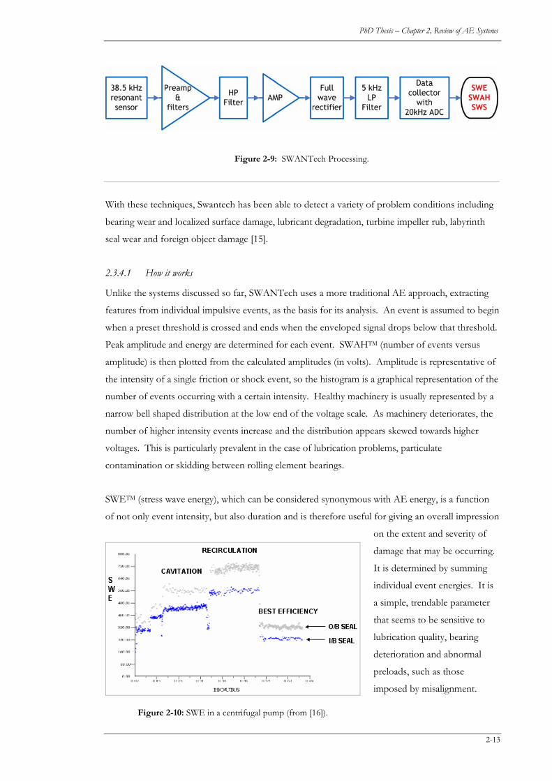
PhD Thesis – Chapter 2, Review of AE Systems
Figure 2-9: SWANTech Processing.
With these techniques, Swantech has been able to detect a variety of problem conditions including
bearing wear and localized surface damage, lubricant degradation, turbine impeller rub, labyrinth
seal wear and foreign object damage [15].
2.3.4.1 How it works
Unlike the systems discussed so far, SWANTech uses a more traditional AE approach, extracting
features from individual impulsive events, as the basis for its analysis. An event is assumed to begin
when a preset threshold is crossed and ends when the enveloped signal drops below that threshold.
Peak amplitude and energy are determined for each event. SWAHTM (number of events versus
amplitude) is then plotted from the calculated amplitudes (in volts). Amplitude is representative of
the intensity of a single friction or shock event, so the histogram is a graphical representation of the
number of events occurring with a certain intensity. Healthy machinery is usually represented by a
narrow bell shaped distribution at the low end of the voltage scale. As machinery deteriorates, the
number of higher intensity events increase and the distribution appears skewed towards higher
voltages. This is particularly prevalent in the case of lubrication problems, particulate
contamination or skidding between rolling element bearings.
SWETM (stress wave energy), which can be considered synonymous with AE energy, is a function
of not only event intensity, but also duration and is therefore useful for giving an overall impression
on the extent and severity of
damage that may be occurring.
It is determined by summing
individual event energies. It is
a simple, trendable parameter
that seems to be sensitive to
lubrication quality, bearing
deterioration and abnormal
preloads, such as those
imposed by misalignment.
Figure 2-10: SWE in a centrifugal pump (from [16]).
2-13

PhD Thesis – Chapter 2, Review of AE Systems
Final failure is normally preceded by a rapid increase in SWE. It can also distinguish between
different types of fluid related problems (Figure 2-10).
2.3.5 SEE – SKF
SKF patented the technology behind their SEE (Spectral Emitted Energy) devices in 1988 [126]1.
Its aim was to overcome the problems incurred when harmonics of fault frequencies overlapped
with the 30-40kHz resonant bandwidth of traditional stress wave devices.
2.3.5.1 How it works
A wideband acoustic emission (piezoelectric) transducer is used to collect the signal that is then
passed through a series of components that give a narrow bandwidth signal around a central
frequency, generally in the 250-350kHz range. Defects will cause an increase in the amplitude of
the filtered signal. It is then passed through four comparators that count how many times the
amplitude exceeds one of four predefined thresholds. The lowest threshold is checked at a rate of
1MHz, the next highest at a rate of 2MHz, the next at 4MHz and the highest at a rate of 8MHz.
These are then totaled together and then divided by the time taken to determine the counts. This
gives an overall weighted count rate, with the higher amplitudes being counted up to eight times
more often than the lowest values. This can be supplied to a digital readout or converted to an
analog voltage for logging.
Figure 2-11: SEE Processing.
1 SKF stopped production of SEE Pens (portable data loggers) in 2003, but the functionality is still included in SKF online analysers. (NC)
2-14
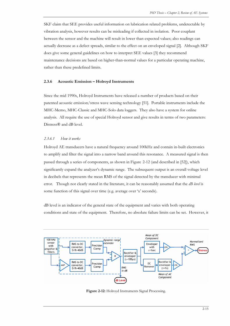
PhD Thesis – Chapter 2, Review of AE Systems
SKF claim that SEE provides useful information on lubrication related problems, undetectable by
vibration analysis, however results can be misleading if collected in isolation. Poor couplant
between the sensor and the machine will result in lower than expected values; also readings can
actually decrease as a defect spreads, similar to the effect on an enveloped signal [2]. Although SKF
does give some general guidelines on how to interpret SEE values [3] they recommend
maintenance decisions are based on higher-than-normal values for a particular operating machine,
rather than these predefined limits.
2.3.6 Acoustic Emission – Holroyd Instruments
Since the mid 1990s, Holroyd Instruments have released a number of products based on their
patented acoustic emission/stress wave sensing technology [51]. Portable instruments include the
MHC-Memo, MHC-Classic and MHC-Solo data loggers. They also have a system for online
analysis. All require the use of special Holroyd sensor and give results in terms of two parameters:
Distress® and dB level.
2.3.6.1 How it works
Holroyd AE transducers have a natural frequency around 100kHz and contain in-built electronics
to amplify and filter the signal into a narrow band around this resonance. A measured signal is then
passed through a series of components, as shown in Figure 2-12 (and described in [52]), which
significantly expand the analyzer’s dynamic range. The subsequent output is an overall voltage level
in decibels that represents the mean RMS of the signal detected by the transducer with minimal
error. Though not clearly stated in the literature, it can be reasonably assumed that the dB level is
some function of this signal over time (e.g. average over ‘x’ seconds).
dB level is an indicator of the general state of the equipment and varies with both operating
conditions and state of the equipment. Therefore, no absolute failure limits can be set. However, it
Figure 2-12: Holroyd Instruments Signal Processing.
2-15
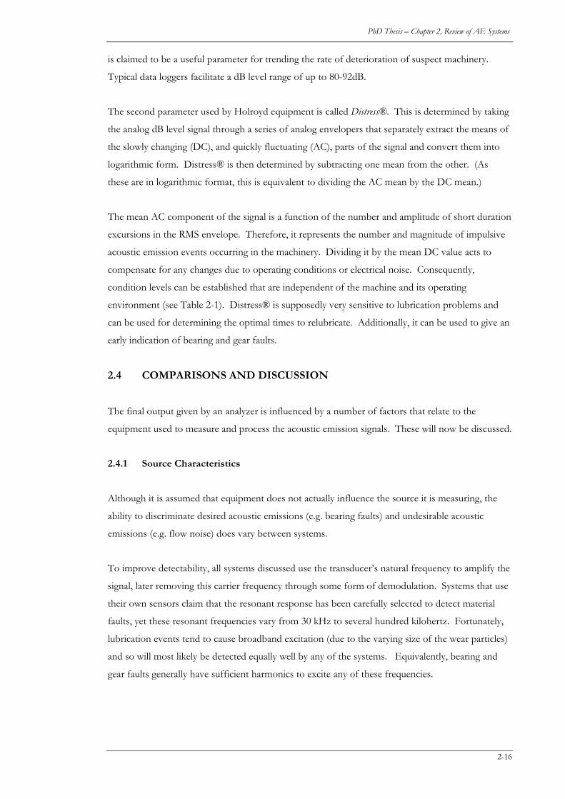
PhD Thesis – Chapter 2, Review of AE Systems
is claimed to be a useful parameter for trending the rate of deterioration of suspect machinery.
Typical data loggers facilitate a dB level range of up to 80-92dB.
The second parameter used by Holroyd equipment is called Distress®. This is determined by taking
the analog dB level signal through a series of analog envelopers that separately extract the means of
the slowly changing (DC), and quickly fluctuating (AC), parts of the signal and convert them into
logarithmic form. Distress® is then determined by subtracting one mean from the other. (As
these are in logarithmic format, this is equivalent to dividing the AC mean by the DC mean.)
The mean AC component of the signal is a function of the number and amplitude of short duration
excursions in the RMS envelope. Therefore, it represents the number and magnitude of impulsive
acoustic emission events occurring in the machinery. Dividing it by the mean DC value acts to
compensate for any changes due to operating conditions or electrical noise. Consequently,
condition levels can be established that are independent of the machine and its operating
environment (see Table 2-1). Distress® is supposedly very sensitive to lubrication problems and
can be used for determining the optimal times to relubricate. Additionally, it can be used to give an
early indication of bearing and gear faults.
2.4 COMPARISONS AND DISCUSSION
The final output given by an analyzer is influenced by a number of factors that relate to the
equipment used to measure and process the acoustic emission signals. These will now be discussed.
2.4.1 Source Characteristics
Although it is assumed that equipment does not actually influence the source it is measuring, the
ability to discriminate desired acoustic emissions (e.g. bearing faults) and undesirable acoustic
emissions (e.g. flow noise) does vary between systems.
To improve detectability, all systems discussed use the transducer’s natural frequency to amplify the
signal, later removing this carrier frequency through some form of demodulation. Systems that use
their own sensors claim that the resonant response has been carefully selected to detect material
faults, yet these resonant frequencies vary from 30 kHz to several hundred kilohertz. Fortunately,
lubrication events tend to cause broadband excitation (due to the varying size of the wear particles)
and so will most likely be detected equally well by any of the systems. Equivalently, bearing and
gear faults generally have sufficient harmonics to excite any of these frequencies.
2-16
PhD Thesis – Chapter 2, Review of AE Systems
Because amplitude attenuates much more at higher frequencies, detection of extraneous, unwanted
signals from other machine components is less likely when using higher frequency sensors,
improving the overall signal to noise ratio. This is particularly important when measuring high-
speed equipment where harmonics of gear mesh and blade pass frequencies could easily move into
the 20-50kHz bandwidth. If these signals are accidentally detected, they may swamp the analyzer’s
dynamic range or make any faults appear larger than they should be. SEE and Holroyd equipment
should be much less prone to these interactions as their resonant frequencies are higher.
Research has indicated that frequency information can be used to discriminate between sources.
Therefore, it would be easier to identify unwanted sources with systems that incorporate some
form of frequency analysis of the time signal (e.g. PeakVue, Spike Energy, SWANTech, SPM with
spectrum options). The user might then be able to collect the data again with a different
bandwidth or sensor location, to remove extraneous signals.
2.4.2 Transducers
As already discussed, signals measured by higher frequency sensors will have a greater SNR.
However, they will most likely be smaller, requiring more sensitive transducers and greater
amplification. Signal conditioning will also have to be less susceptible to instrumentation noise,
but it can be assumed that the manufacturers will have considered these factors. More importantly
from a user’s perspective, at higher frequencies it is crucial to have an adequate couplant (e.g.
silicon grease) between the sensor and work-piece, otherwise most of the signal’s energy will not be
transmitted. Some manufacturers also recommend this when working in the 20-50kHz frequency
range.
Measuring stress waves with an accelerometer seems advantageous: no additional equipment is
required to that used for routine vibration testing. However, there are some problems. As
mentioned earlier, output amplitude is a function of the sensor’s response to an excitation.
Therefore, for the same fault condition, different accelerometers will give different readings. This
prevents any worthwhile comparison being made of components measured by different sensors,
even if all other measuring instrumentation remains unchanged. As even the best sensors can fail
and technology is constantly being updated, there is no guarantee that the same accelerometer type
will always be available. If the relevant sensor was discontinued, years worth of stress wave data
could become worthless and self-defined failure parameters could no longer be used. Although
taking additional measurements with an additional AE (or stress wave) sensor takes more time, it is
likely that the sensor would remain unchanged for the life of the analysis product.
2-17

PhD Thesis – Chapter 2, Review of AE Systems
It is possible to detect stress waves without using the sensor’s resonant response, although signals
are much smaller (10-6V). This approach is used in AE non-destructive testing where tiny signals
are measured by broadband acoustic emission sensors and low noise signal conditioning hardware
Due to the relatively flat response over a larger bandwidth, these sensors are commonly used in
condition monitoring research projects where more features are being extracted from the AE
signal2.
As indicated earlier, sensor location can significantly affect the acoustic emissions measured. If the
transmission path between the source of the acoustic emission and the sensor changes, so will the
amplitude and frequency content of the signal that is detected. Consequently, it is very important
that measurements be taken in the same location every time. If possible, the most direct structural
path between the source and sensor should be used.
2.4.3 Gain and Threshold Level
Most analog systems require the signal to be amplified (or attenuated) so that it is within the
working range of the analog components. This usually requires the user to select appropriate range
or gain settings. If too large a range is selected (compared to the actual range of the signal), then
available resolution will be lost and small signals may be lost in the noise floor. Additionally,
systems that rely on counting the number of bursts above a certain threshold will give erroneously
low values. If too small a range is selected, then the signal will be amplified too much and clipping
of higher amplitude bursts will occur. This will reduce the value of the maximum amplitude
detected to the limit of the range) and effect the frequency content of the signal.
If either the signal amplitude is unknown, or if it varies too much, selection of the correct gain can
be difficult and may result in the loss of signal information. To overcome these problems, Holroyd
instruments have devised a method of accommodating large variations in signal amplitudes without
requiring any gain selection or sacrificing resolution. Remaining technologies may require the user
to try different settings until their signal remains within the limits of the analyzer.
2.4.4 Differences in Functionality
Functionality and the mechanisms by which each system indicate lubrication problems and bearing
faults are summarized in Table 2-1.
2 It is also common to use the AE sensor’s natural frequency to facilitate improved detection of active structural defects. (NC)
2-18
PhD Thesis – Chapter 2, Review of AE Systems
Very few comparisons of available stress wave detection systems have been undertaken. Alfredson
and Mathew evaluated a variety of time domain techniques for monitoring bearings and declared
that although shock pulse was a more reliable indicator of problems than statistical analysis (crest
factor, probability distribution, kurtosis) but required significant operator skill and could not be
used exclusively [9]. Bansal et al compared shock pulse against AE (Peak, RMS and count rate) and
found that the two methods were in good agreement [11]. Both techniques were able to
differentiate between new and reconditioned bearings. Tandon and Nakra concluded that AE was
better than shock pulse and demodulation at measuring very small defects and defects in slow
speed bearings [123]. However, detectability of AE decreased with load, whilst the other
techniques improved. PeakVue has also been reported to provide better detectability that
demodulation [99].
It is well reported that AE levels change with operating conditions, particularly load. Additionally,
as fault conditions deteriorate it is expected that background levels of continuous emission will
increase. In some cases, burst events will remain evident above this background level, whilst at
other times they will disappear into the “noise” floor. For more reliable results, some allowance for
these conditions should be made. SPM and Holroyd equipment do account for these changing
conditions, however in the remaining systems it is up to the user to interpret the data accordingly.
Traditional AE analysis hardware (used by NDT professionals and researchers) has not been
discussed in detail. Some of these alternatives are capable of analyzing AE signals by traditional
vibration tools (e.g. spectra, octave bands etc). Based on DSP hardware, they digitize the analog
signals at 4-20MHz, prior to storage and analysis. This makes them extremely powerful and very
flexible. However, they are not as portable as traditional vibration data loggers, mostly being
incorporated into a desktop PC; the authors are not aware of any currently available variant that can
be integrated into a modern laptop. This should change in the near future, increasing the
availability of AE analysis to a much broader community.
2.5 CONCLUSIONS
Although it is unlikely that acoustic emission will ever replace vibration monitoring, it is a powerful
supplementary tool for detecting incipient faults in machinery. Unfortunately, ensuring reliable,
repeatable and meaningful results can be a complicated process. There are tools on the market that
can simplify these tasks and there is much evidence that these have provided maintenance
professionals with valuable information on many occasions. Black box instruments, like SEE Pen
by SKF and LUB Checker by Holroyd Instruments, are particularly useful for answering simple
questions like "how much lubrication do I need?". The suitability of AE for answering this
particular question has been verified by independent research. Problems begin when these tools
2-19
PhD Thesis – Chapter 2, Review of AE Systems
claim the ability to diagnose more complicated faults with little or no interaction from the condition
monitoring specialist: irrespective of how good the technology, in order to trust the output of these
devices, most technical personnel need to understand what these instruments are doing and how
they derive their results. This can be difficult to find out. The fact that each variant is different but
makes similar claims, adds to confusion and scepticism. Clear explanations of the technology and
comprehensive objective comparisons are needed for these tools to be more widely accepted. This
paper has attempted to initiate this process. Another problem with the present generation of black
box instruments is that they can only identify a limited number of fault types, predominantly
bearing problems. However, future equipment already in development will use more advanced AE
parameters and neural networks to characterise the signals. Automatic diagnoses of machinery
faults should then be significantly more reliable.
The alternative is systems that expose the user to the underlying signals, allowing the analyst to
make a diagnosis. Although this removes the mystery, it does have other drawbacks. Advanced
acoustic emission systems are very expensive and are only produced by a limited number of
manufacturers. They also require the user to become more knowledgeable in acoustic emission
analysis, which has some marked differences from vibration. Issues of where to place sensors, how
to couple them to the equipment and instrumentation sensitivities become even more important
when looking at millivolt or microvolt signals between 10 and 1000kHz. Time waveforms can be
more useful than frequency spectra, so the tools required to analyse them are different.
Furthermore, AE signals are often a function of operating conditions. Finally, to complicate
matters further, there are no standards to guide users in their interpretation of results.
Nevertheless, as the NDT community has shown over the past thirty years, it is possible to
overcome these challenges and the rewards are significant. Advanced AE tools offer the capability
of detecting certain types of faults earlier than currently possible, and can detect problems in
components that presently fail without any warning. This promises safer, cleaner and lower-cost
operating plants. As computers get faster, AE tools will become more numerous and affordable.
When enough collective experience has been gained, standards will be written and standardisation
will follow. Only then, will AE monitoring become as routine as vibration analysis is today.
2.6 POSTSCRIPT (NC)
This review formed the basis of a specification for in-house electronics, DAQ hardware and
software used to collect AE signals from pumps and mechanical seals. Basic requirements
included:
(i) 100-1000kHz bandwidth;
2-20

PhD Thesis – Chapter 2, Review of AE Systems
(ii) 4 channels of simultaneous data digitized at 2-5MHz;
(iii) 20-100dB of gain, some of it programmable;
(iv) The ability to quantify and characterise both discrete and continuous emissions;
(v) The ability to apply and tune the value of floating thresholds;
(vi) Use of generic broadband AE sensors to improve repeatability and independence of results
from sensor response;
(vii) Use of standard or easily understood AE signal features;
(viii) Flexibility to add or change features retrospectively;
(ix) Continuous on-line operation (24 hours a day, 7 days a week) for an indefinite period of
time;
(x) Full exposure to the raw time signal.
The final system, as used to collect some of the data presented in Chapter 9, is summarised in
Appendix B.
2-21
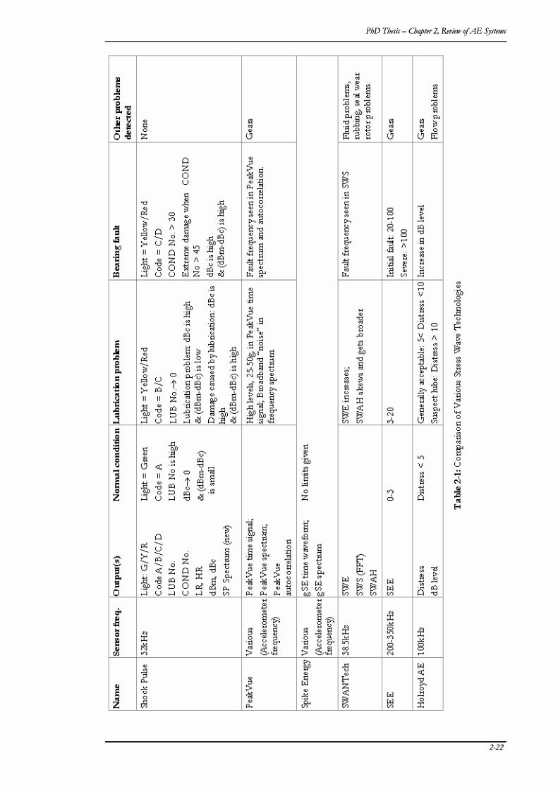
PhD Thesis – Chapter 2, Review of AE Systems PhD Thesis – Chapter 2, Review of AE Systems
2-22 2-22

PhD Thesis – Chapter 2, Review of AE Systems
2-23
3. A
3-1
AEE SSIIGGNNAALL
PPRROOCCEESSSSIINNGG33
The aims of this chapter are to:
(a) Review relevant signal processing theory; and
(b) Introduce the methods used for analysing experimental work presented in later chapters.
Equation Chapter 3 Section 1
3.1 INTRODUCTION
As no two acoustic emission signals will ever be the same, most AE processing is strictly statistical.
In machinery monitoring, this first involves acquiring a large amount of data about an underlying
AE generation mechanism; features are then calculated for this data and plotted; experts peruse the
graphs for changes in feature patterns and make deductions about the underlying conditions (if
known). More recently, neural networks have been used to automate the process of finding
patterns and correlations.
An alternative approach has been taken in this thesis to better relate and quantify AE signals with
test parameters. This involves grouping features into ensembles that correspond to a particular
operating condition or failure mode. Thereafter, statistics describing the feature set are calculated
and trended. Correlations with underlying fault conditions are consequently easy to identify and/or
quantify.
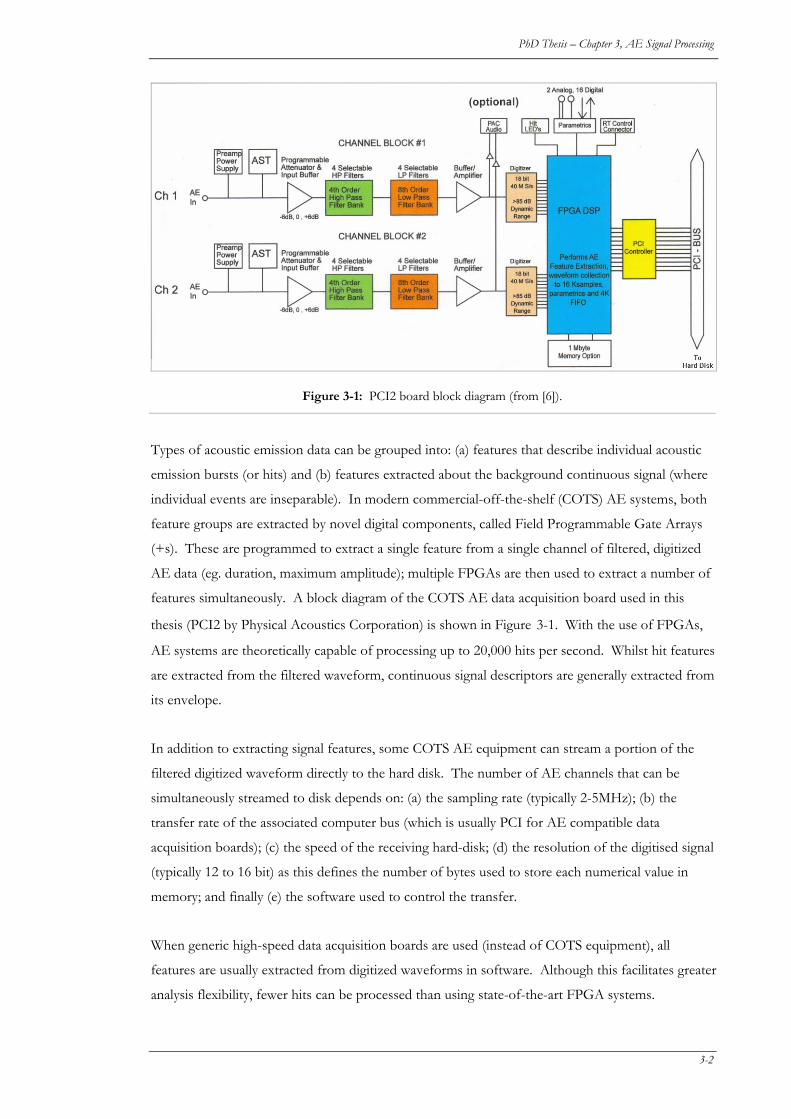
PhD Thesis – Chapter 3, AE Signal Processing
Figure 3-1: PCI2 board block diagram (from [6]).
Types of acoustic emission data can be grouped into: (a) features that describe individual acoustic
emission bursts (or hits) and (b) features extracted about the background continuous signal (where
individual events are inseparable). In modern commercial-off-the-shelf (COTS) AE systems, both
feature groups are extracted by novel digital components, called Field Programmable Gate Arrays
(+s). These are programmed to extract a single feature from a single channel of filtered, digitized
AE data (eg. duration, maximum amplitude); multiple FPGAs are then used to extract a number of
features simultaneously. A block diagram of the COTS AE data acquisition board used in this
thesis (PCI2 by Physical Acoustics Corporation) is shown in Figure 3-1. With the use of FPGAs,
AE systems are theoretically capable of processing up to 20,000 hits per second. Whilst hit features
are extracted from the filtered waveform, continuous signal descriptors are generally extracted from
its envelope.
In addition to extracting signal features, some COTS AE equipment can stream a portion of the
filtered digitized waveform directly to the hard disk. The number of AE channels that can be
simultaneously streamed to disk depends on: (a) the sampling rate (typically 2-5MHz); (b) the
transfer rate of the associated computer bus (which is usually PCI for AE compatible data
acquisition boards); (c) the speed of the receiving hard-disk; (d) the resolution of the digitised signal
(typically 12 to 16 bit) as this defines the number of bytes used to store each numerical value in
memory; and finally (e) the software used to control the transfer.
When generic high-speed data acquisition boards are used (instead of COTS equipment), all
features are usually extracted from digitized waveforms in software. Although this facilitates greater
analysis flexibility, fewer hits can be processed than using state-of-the-art FPGA systems.
3-2
PhD Thesis – Chapter 3, AE Signal Processing
In this research, initial data was collected using generic hardware and custom-written software,
whilst later experiments were conducted with a COTS system. The former option was able to
stream four channels of simultaneous 12/16-bit waveform data at 5MHz, whilst the COTS system
was limited to 2MHz when streaming the same amount of data on similar PC hardware.
3.2 HIT PARAMETERS
Defining a burst as an event that exceeds a certain threshold, traditional features of AE signals used
in this work, as illustrated in Figure 2-2, include:
• Average repetition rate of bursts (interchangeably referred to as event rate, burst rate or hit
rate),
• Amplitude, usually measured in millivolts or dBAE (where 1dBAE=10-6 microvolts)
• Energy (when acquired by the COTS hardware this is called PAC Energy),
• Rise-time (time between first threshold crossing and maximum peak amplitude),
• Counts (number of times an AE burst crosses the threshold),
• Duration.
Values are generally trended to detect abnormalities or visualise rates of change. They may also be
displayed as histograms (number of events versus amplitude, energy, rise time etc), in which
changes in the shape of the curves are analysed; for example, a change from continuous to burst
emission will skew a Gaussian-looking histogram to the right.
Hit data features are a function of the type and value of the selected threshold. Thresholds can be
referred to as fixed, in which case they are set to a specific value for the duration of the test (eg.
40dBAE) or floating, where the threshold level is set as a defined amount (a fixed voltage, or fixed
number of standard deviations) above the background level. Fixed thresholds are typically used
when monitoring static equipment, whilst rotating machinery requires floating thresholds to avoid
swamping acquisition hardware when fluctuations in operating conditions cause the background
signal level to rise.
All experimental work collected for this thesis used floating thresholds. These were set at the
following levels, depending on whether generic or COTS systems were being used:
Generic: 3 standard deviations above the mean
COTS: ASL + 10 dBAE (ASL will be defined shortly)
3-3
PhD Thesis – Chapter 3, AE Signal Processing
3.3 CONTINUOUS SIGNAL PARAMETERS
Traditional AE features for measuring continuous AE signals include RMS, ASL and Absolute
Energy. The manufacturer of the COTS equipment also calculates a feature called Signal Strength.
These terms will be explained in the following sections. All continuous AE features are extracted
by FPGAs from scaled, filtered and enveloped AE signals and require a single input to define the
envelope’s time constant (defined below). Additional statistical and frequency parameters need to
be determined manually from digitized waveforms.
Unless otherwise stated, all features defined in the following sections were calculated for all
experimental data collected.
3.3.1 Traditional Time-dependant Parameters
Traditional analogue demodulation removes high frequency oscillations (the unwanted fast
changing components) from a signal by rectifying it and then applying a time constant that
“smooths out the bumps”. A diagram of this process was given in Figure 2-5. The overall
magnitude and energy of the envelope is related to the magnitude and energy of the raw time signal.
Although significant bursts can be identified, the exact values for arrival times, rise-times and
durations are affected by the time constant; the larger the time constant, the more the signal is
smoothed out and the more envelope values will differ from their true values. Analogue
enveloping can be performed with diodes, peak-hold circuits or operational amplifiers, but the latter
option has a superior dynamic range. In modern COTS systems, FPGAs perform equivalent
processing.
Energy (EN), Power (PN) and RMS (ψN) can be calculated from the digitized signal or envelope (x[N]):
1N2
0
[ ]Ni
E x i=
= ∑−
(3.1)
1
2N
N sE f x i−
= = ⋅0
[ ]Nis
PN t N =⋅ Δ ∑ (3.2)
1 2 1 211 NP −⎡ ⎤ 2
0
[ ]NN
is
x if N
ψ=
⎡ ⎤= = ⋅⎢ ⎥ ⎢ ⎥
⎣ ⎦⎣ ⎦∑ (3.3)
where N is the number of samples acquired from the voltage signal (direct or enveloped) and fs is
the sampling rate for the waveform or digitized envelope.
3-4
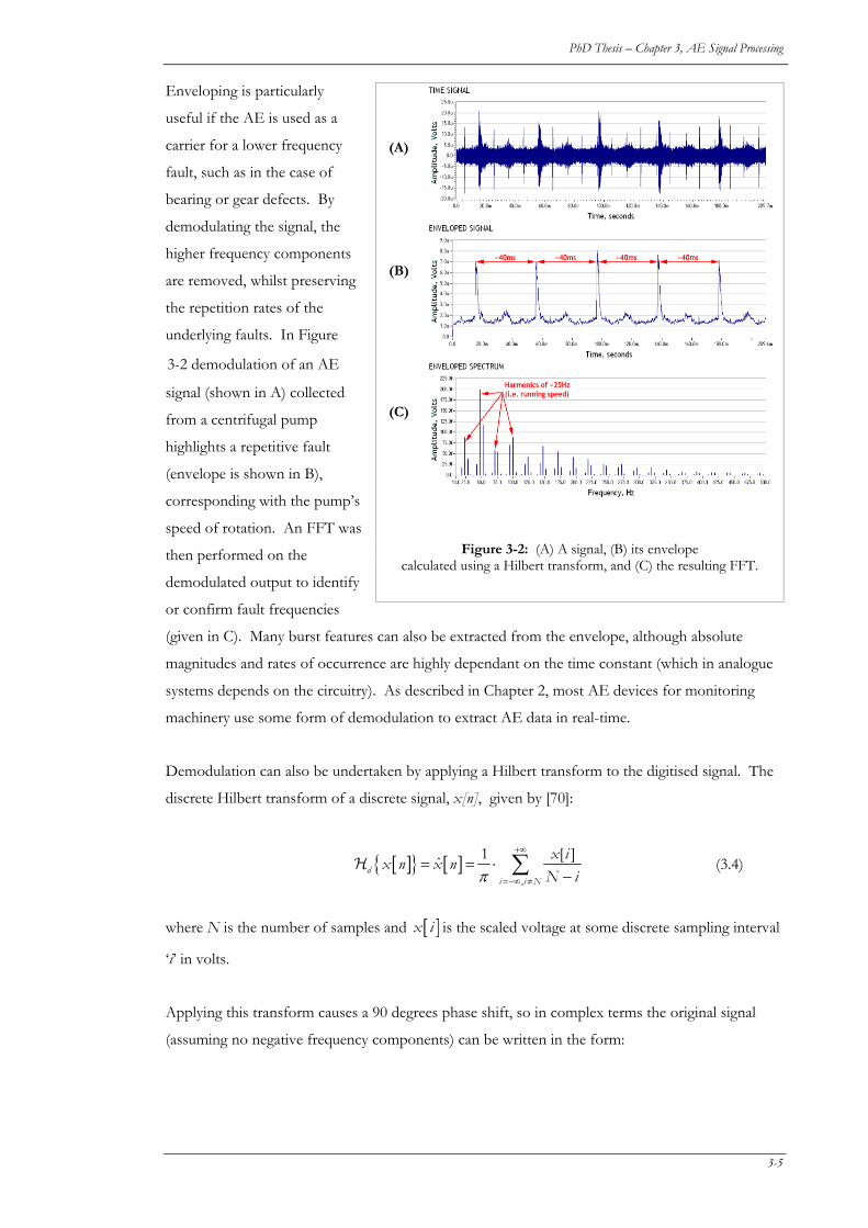
PhD Thesis – Chapter 3, AE Signal Processing
Enveloping is particularly
useful if the AE is used as a
carrier for a lower frequency
fault, such as in the case of
bearing or gear defects. By
demodulating the signal, the
higher frequency components
are removed, whilst preserving
the repetition rates of the
underlying faults. In Figure
3-2 demodulation of an AE
signal (shown in A) collected
from a centrifugal pump
highlights a repetitive fault
(envelope is shown in B),
corresponding with the pump’s
speed of rotation. An FFT was
then performed on the
demodulated output to identify
or confirm fault frequencies
(given in C). Many burst features can also be extracted from the envelope, although absolute
magnitudes and rates of occurrence are highly dependant on the time constant (which in analogue
systems depends on the circuitry). As described in Chapter 2, most AE devices for monitoring
machinery use some form of demodulation to extract AE data in real-time.
(A) (B) (C)
Figure 3-2: (A) A signal, (B) its envelope calculated using a Hilbert transform, and (C) the resulting FFT.
Demodulation can also be undertaken by applying a Hilbert transform to the digitised signal. The
discrete Hilbert transform of a discrete signal, x[n], given by [70]:
[ ]{ } [ ],
ˆdi i N
x n x nN iπ =−∞ ≠
= = ⋅1 [ ]x i+∞
−∑H (3.4)
where N is the number of samples and [ ]x i is the scaled voltage at some discrete sampling interval
‘i’ in volts.
Applying this transform causes a 90 degrees phase shift, so in complex terms the original signal
(assuming no negative frequency components) can be written in the form:
3-5

PhD Thesis – Chapter 3, AE Signal Processing
[ ] [ ] [ ] [ ] [ ] (3.5) ˆ j nz n x n jx n E n e ϖ= + =
The envelope of z(n) is then determined by:
[ ] [ ] [ ] [ ]2 ˆ 2E n z n x n x n= = + (3.6)
Squaring the envelope of the signal, E[n], gives its instantaneous power.
The Hilbert transform of a discrete signal is usually calculated by multiplying the signal’s discrete
Fourier transform by sgn(ω) [70]. Therefore, provided that the signal x(n) is band limited3, its
Hilbert transform, , will have the same amplitude spectrum and auto-correlation function as
the original signal. Unlike a Fourier transform however, a Hilbert transform remains time
dependant.
x̂(n)
In this thesis work, demodulation was used in two ways:
(i) COTS hardware used analogue demodulation to determine continuous AE features of an
AE signal. A time constant of 200ms was typically set.
(ii) Envelopes were used in custom LabVIEW routines that automatically located and
quantified bursts in AE waveform files.
3.3.1.1 PAC Terminology
COTS equipment used (from Physical Acoustic Corporation) refers to continuous AE descriptors
as time dependant features (because they rely on a time constant value from the user). These include
RMS (as defined previously), Absolute Energy, PAC Energy, Signal Strength and Absolute Signal
Level (ASL).
Signal strength is defined as the absolute value of a detected AE signal. It has the same mathematical
description as energy, given in Equation 3.1, but is calculated from the enveloped signal.
PAC Energy also has the same mathematical definition as signal strength and generic energy, but
with reduced resolution. It is a 2-byte feature derived from the “integral of the rectified voltage
3 Given most discrete signals are passed through an anti-aliasing filter prior to digitisation, this assumption
is generally valid.
3-6
PhD Thesis – Chapter 3, AE Signal Processing
signal (i.e. the envelope) over the duration of the AE hit” [5] (rather than 8-bit floating point
numbers used for other energy features).
Absolute Energy is not determined from the envelope, but rather is a measure of the true energy in
the voltage signal, and thus is equivalent to Equation 3.1.
Absolute signal level (ASL) is defined as the time averaged amplitude of the envelope4. In
mathematical terms:
1N
0
[ ]i
E iASL
N==∑
−
(3.7)
where E[i] is the signal envelope in dBAE. The COTS hardware manufacturers calculate floating
thresholds by adding a user-defined fixed amount (typically set to 10dBAE in this work) to the ASL.
Unfortunately, not all features can be accurately determined from a signal’s envelope. Variance and
kurtosis, as well as all frequency descriptors, must be calculated from the filtered, digitized
waveform.
3.3.2 Calculating Statistical Parameters from Raw Waveforms
A discrete sample record is defined as a set of (usually equally spaced) samples collected over a
finite time interval. The duration of the sample record is therefore equal to the time between
successive samples (which equals the inverse of the sampling frequency, fs) multiplied by the
number of samples, N.
Mean, μN, of a signal is a measure of its DC offset and is calculated by:
[ ]11 N
μ−
= ⋅0
Ni
x iN =
∑ (3.8)
where N is the number of samples and [ ]x i is the scaled voltage at some discrete sampling interval
‘i’ in volts.
4 This is deduced from the manufacturer’s literature as no clear definition is given.
3-7
PhD Thesis – Chapter 3, AE Signal Processing
Variance, σ2N (=Std deviation2, σN) is the second statistical moment and indicates the deviation of the
signal around the mean. It is therefore indicative of the spread of burst amplitudes that are smaller
and larger than the baseline level. As the signal mean approaches zero, the standard deviation
approaches the RMS.
[ ]{ }1 22 1 N
Nσ μ−
= ⋅ −0
Ni
x iN =
∑ (3.9)
Kurtosis, KN, (fourth statistical moment) provides an indication of the proportion of time that is
spent at higher amplitudes and is described in its non-dimensional form.
[ ]{ }1 41 N
Nμ−
= ⋅ −40
NiN
K x iNσ =
∑ (3.10)
Kurtosis is commonly calculated by vibration analysts when highly impulsive signals with very small
amplitudes are expected; these types of signals are an early indicator of bearing faults. In AE work,
Kurtosis could potentially describe the type of AE signal being generated; the more impulsive a
signal, the less time is spent at higher amplitudes and the higher the Kurtosis value. On the other
hand, a Gaussian distribution, by which many continuous AE signals can be described, has a
Kurtosis value of three (3). A significant increase in Kurtosis (1-2 orders of magnitude) could
indicate a change from continuous to burst emissions.
Crest Factor, CFN, is the ratio of signal peak to RMS and is also used in vibration analysis for the
detection of highly impulsive bearing faults.
( [ ])max x n
NN
CFψ
= (3.11)
The crest factor of a sine wave is 1.42, whilst a Gaussian distribution is tends to have a value of 1.5.
3.3.2.1 Dealing with very large sample sizes
The equations listed in the previous section require that the entire signal array, x[n], is processed in
one pass. As signals get longer (much greater than 10,000 samples) these equations become more
highly memory intensive, causing computation times to increase substantially. Therefore, as part of
this thesis, the author derived algorithms to calculate the statistics for long signals from smaller
subsets of the signal. The final equations are listed in this section, with full derivations given in
Appendix A.
3-8
PhD Thesis – Chapter 3, AE Signal Processing
If a signal is comprised of N samples, these can be broken up into M sub-sections with S samples
in each. Values for mean, variance, kurtosis and crest factor can be calculated from the following
equations:
1M
μ−
0
[ ]Sk
N
k
Mμ ==
∑ (3.12)
where
1S −
0
[ ][ ] i
S
x ik
Sμ ==
∑ (3.13)
11 1 2M S− −
2
0 0
1 [ ]k i
N
x iS
Mψ = =
⎡ ⎤⎧ ⎫⋅⎨ ⎬⎢ ⎥
⎩ ⎭⎢ ⎥=⎢ ⎥⎢ ⎥⎣ ⎦
∑ ∑ (3.14)
2 2 2 Nσ N Nψ μ= − (3.15)
1 1 1 14 3
3
M S M S
N N N2 2 40 0 0 0
4
[ , ] [ , ]1 4 6k i k i
N NN
x i k x i kK
N Nμ μ ψ μ
σ= = = =
⎪ ⎪⎪ ⎪= ⋅ − ⋅ + −⎨ ⎬⎪ ⎪⎪ ⎪⎩ ⎭
∑∑ ∑∑− − − −⎧ ⎫
(3.16)
where N is the total number of points in the sample record, S is the total number of points in a
section of the sample record, M is the number of sections (N=M × S), i is the position in the
sample within the sub-section (between 0 and M) and k is the number of the sub-section (between
0 and S).
Optimal block size for best performance was determined (by trial and error) to range between 1024
and 4096 points (in powers of 2).
3.3.3 Frequency Parameters
Traditionally, frequency spectra have not been used in acoustic emission analysis because AE is
generally considered to be broadband (energy is distributed across a wide range of frequencies) or
unduly influenced by the natural frequency of the acoustic emission sensor. However, when
looking for rotating equipment faults, demodulated frequency spectra can be useful, particularly if
signals have been collected with wideband sensors (that have no strong resonant frequency).
3-9
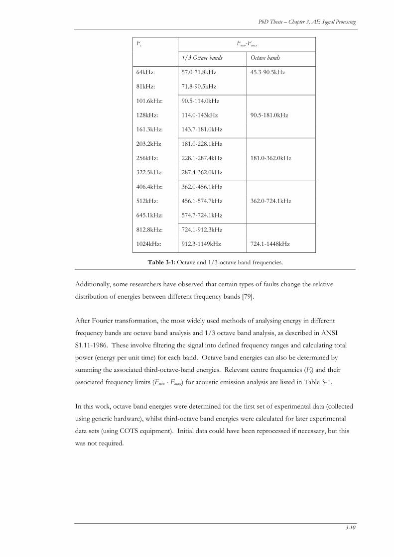
PhD Thesis – Chapter 3, AE Signal Processing
Fc Fmin-Fmax
1/3 Octave bands Octave bands
64kHz: 57.0-71.8kHz 45.3-90.5kHz
81kHz: 71.8-90.5kHz
101.6kHz: 90.5-114.0kHz
128kHz: 114.0-143kHz 90.5-181.0kHz
161.3kHz: 143.7-181.0kHz
203.2kHz 181.0-228.1kHz
256kHz: 228.1-287.4kHz 181.0-362.0kHz
322.5kHz: 287.4-362.0kHz
406.4kHz: 362.0-456.1kHz
512kHz: 456.1-574.7kHz 362.0-724.1kHz
645.1kHz: 574.7-724.1kHz
812.8kHz: 724.1-912.3kHz
1024kHz: 912.3-1149kHz 724.1-1448kHz
Table 3-1: Octave and 1/3-octave band frequencies.
Additionally, some researchers have observed that certain types of faults change the relative
distribution of energies between different frequency bands [79].
After Fourier transformation, the most widely used methods of analysing energy in different
frequency bands are octave band analysis and 1/3 octave band analysis, as described in ANSI
S1.11-1986. These involve filtering the signal into defined frequency ranges and calculating total
power (energy per unit time) for each band. Octave band energies can also be determined by
summing the associated third-octave-band energies. Relevant centre frequencies (Fc) and their
associated frequency limits (Fmin - Fmax) for acoustic emission analysis are listed in Table 3-1.
In this work, octave band energies were determined for the first set of experimental data (collected
using generic hardware), whilst third-octave band energies were calculated for later experimental
data sets (using COTS equipment). Initial data could have been reprocessed if necessary, but this
was not required.
3-10
PhD Thesis – Chapter 3, AE Signal Processing
3.3.4 Joint-time-frequency analysis
Fast Fourier Transformation (FFT) destroys all time information: a FFT calculation returns all
frequencies that are present in the signal irrespective of whether they exist for its entire duration or
are only transitory. Therefore, in general, FFT analysis should only be performed on stationary and
ergodic signals.
Burst AE signals are neither ergodic, nor stationary. In many cases, nor are continuous emissions.
Therefore over the last decade many researchers have attempted to characterise AE signals by more
advanced techniques such as wavelets [43, 62, 87, 119, 125, 127], Wigner-Ville functions [32], short-
time Fourier Transforms (STFT) [131] and Kalman filtering [88], of which wavelets seem to be the
most popular. Known collectively as “Joint Time Frequency Analysis” (JTFA), these algorithms
analyse how frequencies change with time and are more computationally intensive than standard
frequency analysis.
For all JTFA techniques, the amount of time-frequency information being analysed (known as the
time-bandwidth product) is limited by the uncertainty principle [13]:
1
4t f
πΔ ⋅ Δ ≥ (3.17)
This relationship necessitates that for a given sample set, any improvement in time resolution can
only occur as a reduction in frequency resolution and vice versa.
STFTs can be thought of as simply an extension of traditional FFTs; the time-frequency space is
effectively divided into a number of equal blocks and then a windowed Fourier transform is
performed on each block. Blocks are overlapped slightly to overcome errors caused by applying
the window function. Results are typically displayed on a contour plot, called a spectrogram, or a 3-
D x-y-z (time-frequency-amplitude) plot. Unfortunately, ultimate resolution is limited by equation
3.17, so the only way to increase temporal resolution is to decrease frequency resolution and vice
versa. STFTs are useful because they are easy to compute and interpret.
Continuous-time wavelet transforms (CWT) on the other hand, are special mathematical functions
that split a signal into non-uniform sections (windows), localised in time and scale [94]. Scale is
related to, but not synonymous with, frequency. To determine values for each window, wavelet
transformation dilates and translates a basis function (called a mother wavelet). The CWT is simply
the cross correlation of the time signal, x[n], with this dilated and translated wavelet. The results of
this process are then displayed as a spectrogram or xyz plot.
3-11
PhD Thesis – Chapter 3, AE Signal Processing
A wavelet transform has the (discrete) form:
11
2N
x i bψ−
−,
0
[ ]a bi
W a x ia=
−⎛ ⎞= ⋅ ⎟⎜⎝ ⎠
∑ (3.18)
where ( )tψ is the basis function, a is the scale and b is the translation in time.
The centre frequency of the mother wavelet can be determined from its frequency response, but
can be roughly approximated as the Nyquist frequency (half of the sampling rate in Hertz).
Thereafter the centre frequency decreases (is translated) by a factor of two.
Energy in a particular wavelet band, or band energy (Ea), can be calculated by:
2x
bE W= ∑ ,a ab
(3.19)
As wavelet transformation preserves the energy of the original signal, total energy, E, can be
determined by integrating (or in discrete terms, summing) the individual bands.
2xWE ,
2a baE
a a= =∑ ∑∑ (3.20)
CWT generally has superior resolution over STFT because of its non-uniform division of time and
scale: at higher scales, signals are divided into very short blocks of time, allowing identification of
very quick, impulsive events, whilst at lower scales they are highly localised in scale, facilitating
identification of specific frequencies. This makes them incredibly useful for identifying sharp (i.e.
high frequency) bursts and discontinuities that may be masked by larger stationary signals or noise
(low frequency). Unfortunately, a CWT generally takes more time to calculate than an STFT.
A computationally lighter alternative to CWT is the discrete wavelet transformation (DWT), called
the Mallat algorithm, which uses special orthogonal filter banks to divide the signal into scale bands.
Many wavelets also facilitate perfect reconstruction of the original signal from its component parts
which means that any signal can be split up into sections, unwanted or unused parts of the signal
then removed, and the signal rebuilt without affecting the important or desired information. This is
not possible with traditional band-pass filters (i.e. octave band analysis, STFT). Discrete wavelet
analysis and its application to signal denoising is discussed further in Chapter 4.
In this thesis, discrete wavelets were used to separate AE bursts from continuous emissions. A
flowchart of the process used to extract denoised AE bursts is given in Appendix C.1.
3-12
PhD Thesis – Chapter 3, AE Signal Processing
National Instrument’s Signal Processing Toolbox for LabVIEW includes various algorithms for
denoising and detrending signals depending on the type of background noise that is
“contaminating” the signal [94]. Unfortunately, there are no clear guidelines as to which wavelet
should be applied. Selection is data dependant and therefore the most appropriate wavelet function
can only be ascertained through trial and error. Most prior AE work used various Daubechies [64,
77, 87, 127] or Haar wavelet functions for discrete wavelet processing [92], and Gabor (otherwise
known as Morlet) or Meyer continuous wavelet functions [43, 117]. Some guidelines developed
for this research are presented in Chapter 4.
Unless otherwise stated, in this thesis waveform signals were processed by applying either 0.1-
1MHz or 0.1-0.4MHz bandpass digital filters and then denoised using a Haar wavelet function.
Denoised signals were subsequently enveloped by the Hilbert function to simplify automated burst
identification. However, burst parameters (peak, RMS etc.) were extracted from the denoised
signals and not their envelopes.
The Haar mother wavelet has the form:
1 0 0.5t+ ≤ ≤⎧( ) 1 0.5 1
0w t t
otherwise
⎪= − < ≤⎨⎪⎩
(3.21)
( )For daughter wavelets: , ( ) 2 2aa bw t w t b for all a,b= ⋅ − (3.22)
3.4 ENSEMBLE STATISTICS
An ensemble is a collection of sample records. In signal processing of time based data, statistics
can either be determined on the sample records directly, in which case the statistics describe
features of the underlying signal at a temporal location, or on an ensemble, which then describes
how the signal varies across the sample records.
In this thesis, ensemble averages are calculated for all AE features. A bar over a parameter denotes
an ensemble, rather than sample statistic (i.e. mμ is the sample record mean based calculated on n
samples, whilst mμ denotes the ensemble mean calculated on m ensembles).
3.4.1 Confidence limits
A signal is described as being stationary if its sample record statistics are temporally static. In
mathematical terms:
3-13
PhD Thesis – Chapter 3, AE Signal Processing
( ) [ ] ME x n = μ (3.23)
( ) 2 2ME σ σ= (3.24)
where M is the number of sample records in the ensemble.
A signal is termed ergodic if any single ensemble statistic can be used to describe the signal. Acoustic
emission signals are rarely ergodic and often non-stationary, especially if signal blocks are short
(<100,000 samples). Therefore, for ensemble averaging to be useful, confidence limits are required
to quantify the spread of values that make up the sample records in the ensemble.
All statistical equations quoted so far assume that values being analysed (the underlying data in the
case of sample record statistics, or the statistics themselves in the case of ensemble averages) vary
according to a normal distribution. Based on the same assumption, confidence limits for the
respective ensemble means and ensemble variances can also be established.
Two sided 100%(1-α) confidence limits on the mean of a normal distribution, with unknown
population variance can be determined from the t distribution:
/2, 1 /2, 1M M M M MM
t tM M
α Mαμ σ μμ− σ−− +
≤ ≤ (3.25)
where Mμ is the mean of the ensemble statistics, S is the standard deviation of the ensemble
statistics, M is the number of records in the dataset and tα/2,M-1 is the t distribution with M-1 degrees
of freedom for the desired confidence interval.
The less variable the statistics between each sample set, the tighter the confidence limits.
Conversely, large confidence limits indicate significant variability in the statistics between measured
features. This is either attributable to an insufficient number of features calculated, or due to an
increased variability in the underlying data as may be caused by very impulsive, highly non-
stationary acoustic emission signals.
In this thesis, unless otherwise stated, line graphs show the ensemble mean and 90% confidence
limits of a particular AE feature. As baseline levels vary significantly between different pumps
and/or speeds, ensemble averages are normalised by the mean ensemble value that corresponds to
particular condition (eg. BEP or max-NPSHA).
3-14
4. DDEENNOOIISSIINNGG
AAEE DDAATTAA 44 The aim of this chapter is to present methods of denoising various forms of AE data so that
information pertinent to unfavourable operating conditions or incipient mechanical failure can be
detected and accurately quantified.
Abstract
Acoustic emission (AE) data collected from operational equipment comprises of genuine
information, pertaining to AE sources of interest, and noise. A variety of signal processing
techniques have been developed over the past 20 years to denoise condition-monitoring data, with
varying degrees of success when applied to AE analysis. This is, in part, because what constitutes
noise and what is regarded as genuine data changes from one application to the next; thus it is
impossible to develop a single set of processing techniques that will be applicable in all situations.
Consequently, publications relating to noise management tend to be application specific, and most
relate to traditional AE applications such as crack monitoring. To simplify the process of acquiring
useful AE information from rotating machines, this paper presents examples of how hit filtering,
averaging and wavelet denoising were used by the author to improve the signal to noise ratio of AE
data collected from centrifugal pumps.
4.1 INTRODUCTION
Post processing techniques are typically applied to extract either the source signal of interest, or
some characteristic of this signal, from waveform data or a feature-set. Assuming that noise is
4-1
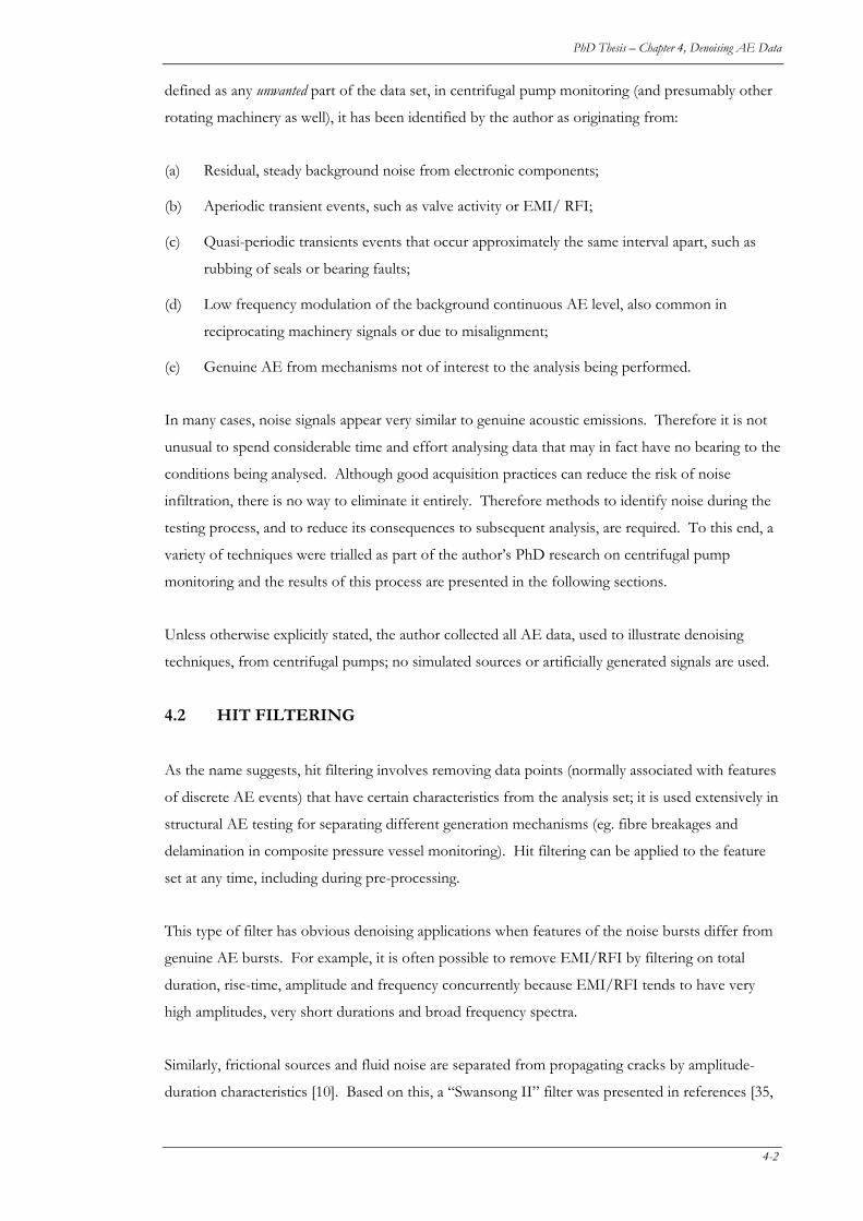
PhD Thesis – Chapter 4, Denoising AE Data
defined as any unwanted part of the data set, in centrifugal pump monitoring (and presumably other
rotating machinery as well), it has been identified by the author as originating from:
(a) Residual, steady background noise from electronic components;
(b) Aperiodic transient events, such as valve activity or EMI/ RFI;
(c) Quasi-periodic transients events that occur approximately the same interval apart, such as
rubbing of seals or bearing faults;
(d) Low frequency modulation of the background continuous AE level, also common in
reciprocating machinery signals or due to misalignment;
(e) Genuine AE from mechanisms not of interest to the analysis being performed.
In many cases, noise signals appear very similar to genuine acoustic emissions. Therefore it is not
unusual to spend considerable time and effort analysing data that may in fact have no bearing to the
conditions being analysed. Although good acquisition practices can reduce the risk of noise
infiltration, there is no way to eliminate it entirely. Therefore methods to identify noise during the
testing process, and to reduce its consequences to subsequent analysis, are required. To this end, a
variety of techniques were trialled as part of the author’s PhD research on centrifugal pump
monitoring and the results of this process are presented in the following sections.
Unless otherwise explicitly stated, the author collected all AE data, used to illustrate denoising
techniques, from centrifugal pumps; no simulated sources or artificially generated signals are used.
4.2 HIT FILTERING
As the name suggests, hit filtering involves removing data points (normally associated with features
of discrete AE events) that have certain characteristics from the analysis set; it is used extensively in
structural AE testing for separating different generation mechanisms (eg. fibre breakages and
delamination in composite pressure vessel monitoring). Hit filtering can be applied to the feature
set at any time, including during pre-processing.
This type of filter has obvious denoising applications when features of the noise bursts differ from
genuine AE bursts. For example, it is often possible to remove EMI/RFI by filtering on total
duration, rise-time, amplitude and frequency concurrently because EMI/RFI tends to have very
high amplitudes, very short durations and broad frequency spectra.
Similarly, frictional sources and fluid noise are separated from propagating cracks by amplitude-
duration characteristics [10]. Based on this, a “Swansong II” filter was presented in references [35,
4-2
PhD Thesis – Chapter 4, Denoising AE Data
36] to extract crack-generated AE from fluid noise when verifying tank and pressure vessel
integrity; this filter removes all data within 0.5 seconds of a “telltale” hit, defined by the following
criteria:
Amplitude (in dBAE) Duration
< 5dB above threshold AND >2000 μs
OR <10dB above threshold AND >3500 μs
OR <15dB above threshold AND >4500 μs
Figure 4-1 shows how hit filtering can be used in a traditional AE application (crack propagation in
a pressure vessel). Red and green points signify AE hits measured during a pressure test of a steel
cylinder. Different types of noise were removed by identifying hits with certain combined
amplitude, duration or energy characteristics. These are shown as red points. (The coloured lines
indicate probable varieties of noise.) Remaining hits are shown in green; these were subsequently
analysed to ascertain the nature, severity and location of the potential crack. In this example,
probable EMI has not been removed by hit filtering and thus needs to be removed by alternative
processing.
Figure 4-1: Different amplitude-duration characteristics of AE hits. Data has been processed by a Swansong II filter but probable EMI noise still remains. (PUMAnalysis software courtesy
of Imes Group Ltd.)
SATURATION: removed by filtering hits
with Duration ≥106
Probable EMI noise
FLUID NOISE: removed by
Swansong filter
FRICTION NOISE (removed by
Swansong filter)
Either side of a tell-tale hit
SMALL EVENTS: removed by filtering hits with Amplitude <46dB
4-3
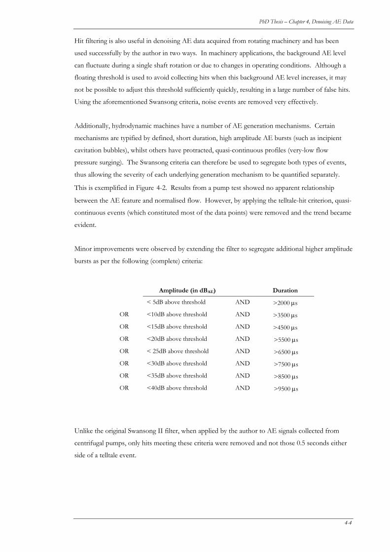
PhD Thesis – Chapter 4, Denoising AE Data
Hit filtering is also useful in denoising AE data acquired from rotating machinery and has been
used successfully by the author in two ways. In machinery applications, the background AE level
can fluctuate during a single shaft rotation or due to changes in operating conditions. Although a
floating threshold is used to avoid collecting hits when this background AE level increases, it may
not be possible to adjust this threshold sufficiently quickly, resulting in a large number of false hits.
Using the aforementioned Swansong criteria, noise events are removed very effectively.
Additionally, hydrodynamic machines have a number of AE generation mechanisms. Certain
mechanisms are typified by defined, short duration, high amplitude AE bursts (such as incipient
cavitation bubbles), whilst others have protracted, quasi-continuous profiles (very-low flow
pressure surging). The Swansong criteria can therefore be used to segregate both types of events,
thus allowing the severity of each underlying generation mechanism to be quantified separately.
This is exemplified in Figure 4-2. Results from a pump test showed no apparent relationship
between the AE feature and normalised flow. However, by applying the telltale-hit criterion, quasi-
continuous events (which constituted most of the data points) were removed and the trend became
evident.
Minor improvements were observed by extending the filter to segregate additional higher amplitude
bursts as per the following (complete) criteria:
Amplitude (in dBAE) Duration
< 5dB above threshold AND >2000 μs
OR <10dB above threshold AND >3500 μs
OR <15dB above threshold AND >4500 μs
OR <20dB above threshold AND >5500 μs
OR < 25dB above threshold AND >6500 μs
OR <30dB above threshold AND >7500 μs
OR <35dB above threshold AND >8500 μs
OR <40dB above threshold AND >9500 μs
Unlike the original Swansong II filter, when applied by the author to AE signals collected from
centrifugal pumps, only hits meeting these criteria were removed and not those 0.5 seconds either
side of a telltale event.
4-4
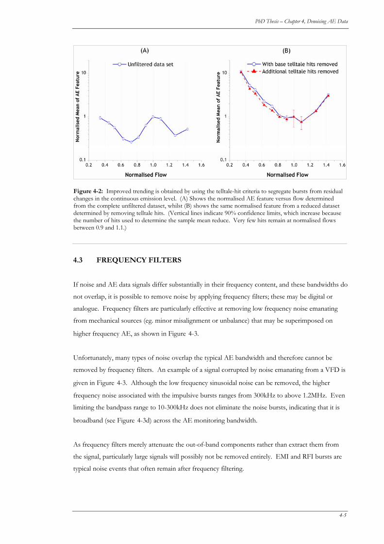
PhD Thesis – Chapter 4, Denoising AE Data
Figure 4-2: Improved trending is obtained by using the telltale-hit criteria to segregate bursts from residual changes in the continuous emission level. (A) Shows the normalised AE feature versus flow determined from the complete unfiltered dataset, whilst (B) shows the same normalised feature from a reduced dataset determined by removing telltale hits. (Vertical lines indicate 90% confidence limits, which increase because the number of hits used to determine the sample mean reduce. Very few hits remain at normalised flows between 0.9 and 1.1.)
4.3 FREQUENCY FILTERS
If noise and AE data signals differ substantially in their frequency content, and these bandwidths do
not overlap, it is possible to remove noise by applying frequency filters; these may be digital or
analogue. Frequency filters are particularly effective at removing low frequency noise emanating
from mechanical sources (eg. minor misalignment or unbalance) that may be superimposed on
higher frequency AE, as shown in Figure 4-3.
Unfortunately, many types of noise overlap the typical AE bandwidth and therefore cannot be
removed by frequency filters. An example of a signal corrupted by noise emanating from a VFD is
given in Figure 4-3. Although the low frequency sinusoidal noise can be removed, the higher
frequency noise associated with the impulsive bursts ranges from 300kHz to above 1.2MHz. Even
limiting the bandpass range to 10-300kHz does not eliminate the noise bursts, indicating that it is
broadband (see Figure 4-3d) across the AE monitoring bandwidth.
As frequency filters merely attenuate the out-of-band components rather than extract them from
the signal, particularly large signals will possibly not be removed entirely. EMI and RFI bursts are
typical noise events that often remain after frequency filtering.
4-5
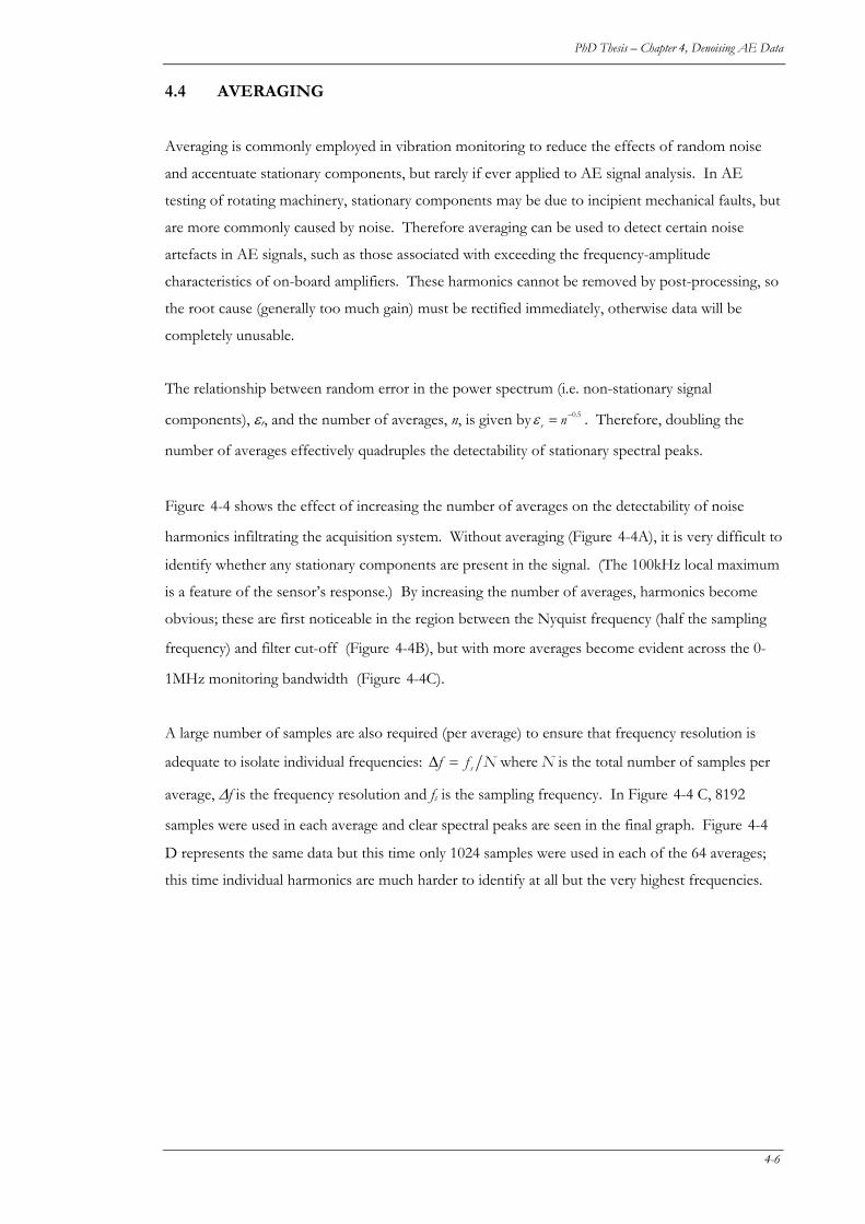
PhD Thesis – Chapter 4, Denoising AE Data
4.4 AVERAGING
Averaging is commonly employed in vibration monitoring to reduce the effects of random noise
and accentuate stationary components, but rarely if ever applied to AE signal analysis. In AE
testing of rotating machinery, stationary components may be due to incipient mechanical faults, but
are more commonly caused by noise. Therefore averaging can be used to detect certain noise
artefacts in AE signals, such as those associated with exceeding the frequency-amplitude
characteristics of on-board amplifiers. These harmonics cannot be removed by post-processing, so
the root cause (generally too much gain) must be rectified immediately, otherwise data will be
completely unusable.
The relationship between random error in the power spectrum (i.e. non-stationary signal
components), εr, and the number of averages, n, is given by . Therefore, doubling the
number of averages effectively quadruples the detectability of stationary spectral peaks.
0.5r nε −=
Figure 4-4 shows the effect of increasing the number of averages on the detectability of noise
harmonics infiltrating the acquisition system. Without averaging (Figure 4-4A), it is very difficult to
identify whether any stationary components are present in the signal. (The 100kHz local maximum
is a feature of the sensor’s response.) By increasing the number of averages, harmonics become
obvious; these are first noticeable in the region between the Nyquist frequency (half the sampling
frequency) and filter cut-off (Figure 4-4B), but with more averages become evident across the 0-
1MHz monitoring bandwidth (Figure 4-4C).
A large number of samples are also required (per average) to ensure that frequency resolution is
adequate to isolate individual frequencies: sf f NΔ = where N is the total number of samples per
average, Δf is the frequency resolution and fs is the sampling frequency. In Figure 4-4 C, 8192
samples were used in each average and clear spectral peaks are seen in the final graph. Figure 4-4
D represents the same data but this time only 1024 samples were used in each of the 64 averages;
this time individual harmonics are much harder to identify at all but the very highest frequencies.
4-6
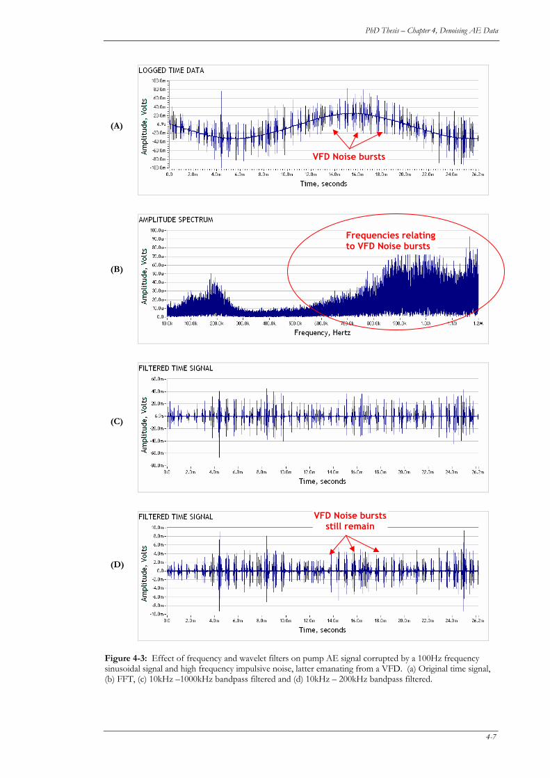
PhD Thesis – Chapter 4, Denoising AE Data
(A)
VFD Noise bursts
Frequencies relating to VFD Noise bursts
(B)
(C)
VFD Noise bursts still remain
(D)
Figure 4-3: Effect of frequency and wavelet filters on pump AE signal corrupted by a 100Hz frequency sinusoidal signal and high frequency impulsive noise, latter emanating from a VFD. (a) Original time signal, (b) FFT, (c) 10kHz –1000kHz bandpass filtered and (d) 10kHz – 200kHz bandpass filtered.
4-7
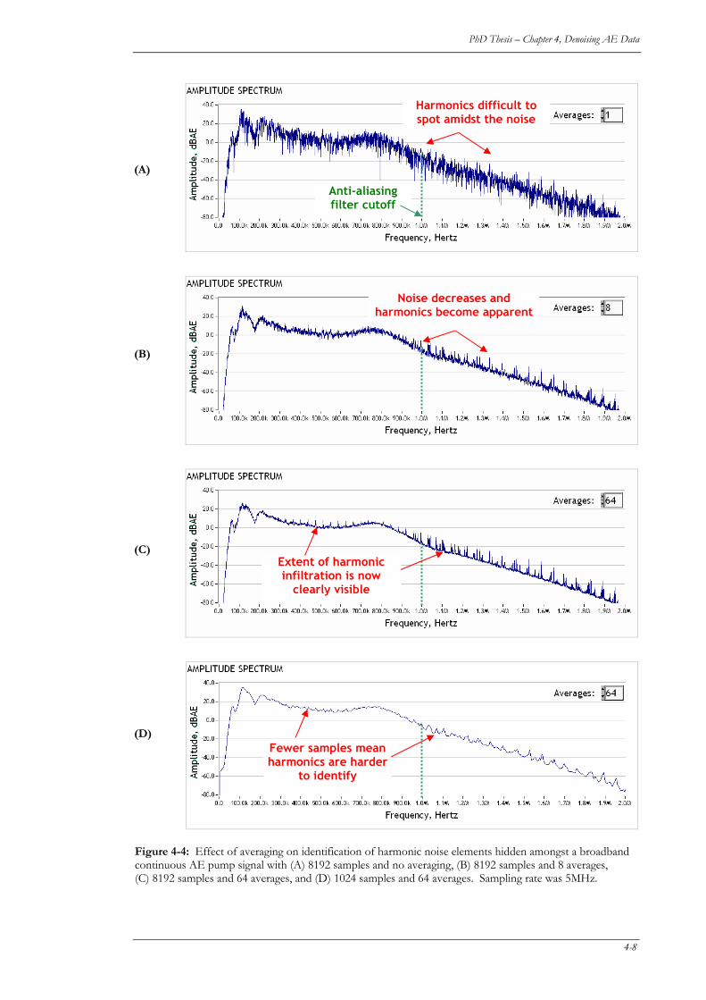
PhD Thesis – Chapter 4, Denoising AE Data
Harmonics difficult to spot amidst the noise
Noise decreases and harmonics become apparent
Extent of harmonic infiltration is now
clearly visible
Fewer samples mean harmonics are harder
to identify
Anti-aliasing filter cutoff
(A)
(B)
(C)
(D)
Figure 4-4: Effect of averaging on identification of harmonic noise elements hidden amongst a broadband continuous AE pump signal with (A) 8192 samples and no averaging, (B) 8192 samples and 8 averages, (C) 8192 samples and 64 averages, and (D) 1024 samples and 64 averages. Sampling rate was 5MHz.
4-8
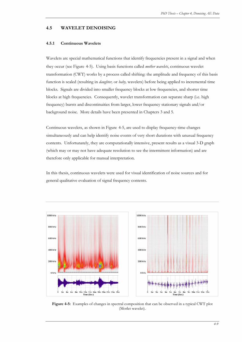
PhD Thesis – Chapter 4, Denoising AE Data
4.5 WAVELET DENOISING
4.5.1 Continuous Wavelets
Wavelets are special mathematical functions that identify frequencies present in a signal and when
they occur (see Figure 4-5). Using basis functions called mother wavelets, continuous wavelet
transformation (CWT) works by a process called shifting: the amplitude and frequency of this basis
function is scaled (resulting in daughter, or baby, wavelets) before being applied to incremental time
blocks. Signals are divided into smaller frequency blocks at low frequencies, and shorter time
blocks at high frequencies. Consequently, wavelet transformation can separate sharp (i.e. high
frequency) bursts and discontinuities from larger, lower frequency stationary signals and/or
background noise. More details have been presented in Chapters 3 and 5.
Continuous wavelets, as shown in Figure 4-5, are used to display frequency-time changes
simultaneously and can help identify noise events of very short durations with unusual frequency
contents. Unfortunately, they are computationally intensive, present results as a visual 3-D graph
(which may or may not have adequate resolution to see the intermittent information) and are
therefore only applicable for manual interpretation.
In this thesis, continuous wavelets were used for visual identification of noise sources and for
general qualitative evaluation of signal frequency contents.
Figure 4-5: Examples of changes in spectral composition that can be observed in a typical CWT plot (Morlet wavelet).
4-9
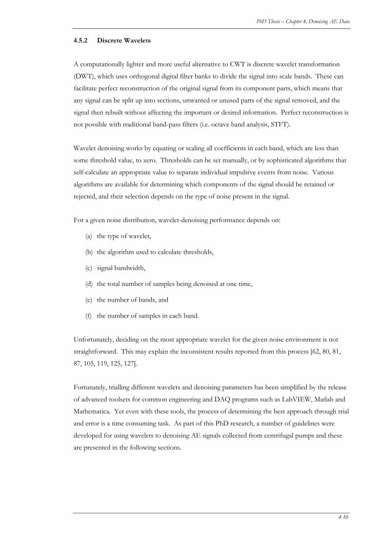
PhD Thesis – Chapter 4, Denoising AE Data
4.5.2 Discrete Wavelets
A computationally lighter and more useful alternative to CWT is discrete wavelet transformation
(DWT), which uses orthogonal digital filter banks to divide the signal into scale bands. These can
facilitate perfect reconstruction of the original signal from its component parts, which means that
any signal can be split up into sections, unwanted or unused parts of the signal removed, and the
signal then rebuilt without affecting the important or desired information. Perfect reconstruction is
not possible with traditional band-pass filters (i.e. octave band analysis, STFT).
Wavelet denoising works by equating or scaling all coefficients in each band, which are less than
some threshold value, to zero. Thresholds can be set manually, or by sophisticated algorithms that
self-calculate an appropriate value to separate individual impulsive events from noise. Various
algorithms are available for determining which components of the signal should be retained or
rejected, and their selection depends on the type of noise present in the signal.
For a given noise distribution, wavelet-denoising performance depends on:
(a) the type of wavelet,
(b) the algorithm used to calculate thresholds,
(c) signal bandwidth,
(d) the total number of samples being denoised at one time,
(e) the number of bands, and
(f) the number of samples in each band.
Unfortunately, deciding on the most appropriate wavelet for the given noise environment is not
straightforward. This may explain the inconsistent results reported from this process [62, 80, 81,
87, 105, 119, 125, 127].
Fortunately, trialling different wavelets and denoising parameters has been simplified by the release
of advanced toolsets for common engineering and DAQ programs such as LabVIEW, Matlab and
Mathematica. Yet even with these tools, the process of determining the best approach through trial
and error is a time consuming task. As part of this PhD research, a number of guidelines were
developed for using wavelets to denoising AE signals collected from centrifugal pumps and these
are presented in the following sections.
4-10
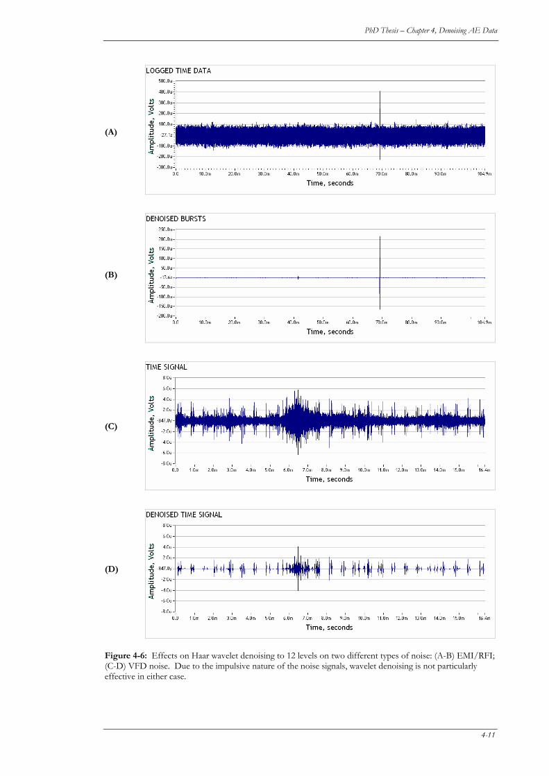
PhD Thesis – Chapter 4, Denoising AE Data
(A)
(B)
Figure 4-6: Effects on Haar wavelet denoising to 12 levels on two different types of noise: (A-B) EMI/RFI; (C-D) VFD noise. Due to the impulsive nature of the noise signals, wavelet denoising is not particularly effective in either case.
(C)
(D)
4-11
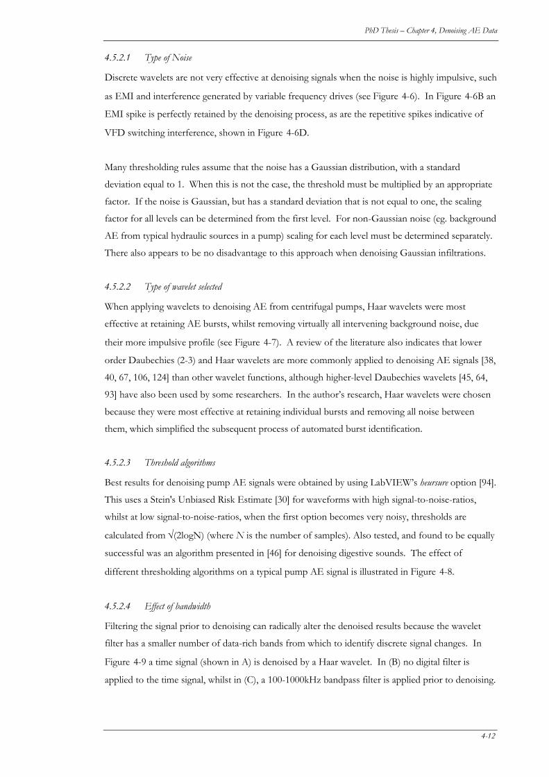
PhD Thesis – Chapter 4, Denoising AE Data
4.5.2.1 Type of Noise
Discrete wavelets are not very effective at denoising signals when the noise is highly impulsive, such
as EMI and interference generated by variable frequency drives (see Figure 4-6). In Figure 4-6B an
EMI spike is perfectly retained by the denoising process, as are the repetitive spikes indicative of
VFD switching interference, shown in Figure 4-6D.
Many thresholding rules assume that the noise has a Gaussian distribution, with a standard
deviation equal to 1. When this is not the case, the threshold must be multiplied by an appropriate
factor. If the noise is Gaussian, but has a standard deviation that is not equal to one, the scaling
factor for all levels can be determined from the first level. For non-Gaussian noise (eg. background
AE from typical hydraulic sources in a pump) scaling for each level must be determined separately.
There also appears to be no disadvantage to this approach when denoising Gaussian infiltrations.
4.5.2.2 Type of wavelet selected
When applying wavelets to denoising AE from centrifugal pumps, Haar wavelets were most
effective at retaining AE bursts, whilst removing virtually all intervening background noise, due
their more impulsive profile (see Figure 4-7). A review of the literature also indicates that lower
order Daubechies (2-3) and Haar wavelets are more commonly applied to denoising AE signals [38,
40, 67, 106, 124] than other wavelet functions, although higher-level Daubechies wavelets [45, 64,
93] have also been used by some researchers. In the author’s research, Haar wavelets were chosen
because they were most effective at retaining individual bursts and removing all noise between
them, which simplified the subsequent process of automated burst identification.
4.5.2.3 Threshold algorithms
Best results for denoising pump AE signals were obtained by using LabVIEW’s heursure option [94].
This uses a Stein's Unbiased Risk Estimate [30] for waveforms with high signal-to-noise-ratios,
whilst at low signal-to-noise-ratios, when the first option becomes very noisy, thresholds are
calculated from √(2logN) (where N is the number of samples). Also tested, and found to be equally
successful was an algorithm presented in [46] for denoising digestive sounds. The effect of
different thresholding algorithms on a typical pump AE signal is illustrated in Figure 4-8.
4.5.2.4 Effect of bandwidth
Filtering the signal prior to denoising can radically alter the denoised results because the wavelet
filter has a smaller number of data-rich bands from which to identify discrete signal changes. In
Figure 4-9 a time signal (shown in A) is denoised by a Haar wavelet. In (B) no digital filter is
applied to the time signal, whilst in (C), a 100-1000kHz bandpass filter is applied prior to denoising.
4-12
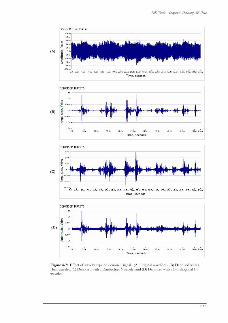
PhD Thesis – Chapter 4, Denoising AE Data
(A)
(B)
(C)
(D)
Figure 4-7: Effect of wavelet type on denoised signal. (A) Original waveform, (B) Denoised with a Haar wavelet, (C) Denoised with a Daubechies 6 wavelet and (D) Denoised with a Biorthogonal 1-3 wavelet.
4-13
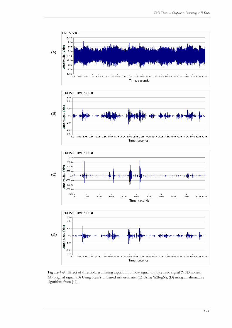
PhD Thesis – Chapter 4, Denoising AE Data
(A)
(B)
Figure 4-8: Effect of threshold estimating algorithm on low signal to noise ratio signal (VFD noise): (A) original signal; (B) Using Stein’s unbiased risk estimate, (C) Using √(2logN), (D) using an alternative algorithm from [46].
(C)
(D)
4-14
PhD Thesis – Chapter 4, Denoising AE Data
(A)
(B)
(C)
Figure 4-9: Effect of filtering on the final denoised signal. (A) Original signal, (B) After denoising by Haar wavelet; (C) 100-1000kHz digital filter applied prior to denoising by Haar wavelet.
In the latter bandwidth VFD noise dominates and is retained by the wavelet algorithm, whilst (by
comparison) less impulsive, genuine AE data is removed.
4.5.2.5 Signal length
Signals must be sufficiently long so that statistical properties of the background noise can be
properly estimated. Windows need to be much longer than individual discrete bursts, and therefore
in acoustic emission work, the author has found that waveforms must have at least 16384 samples
(fs= 2-5MHz) for wavelet denoising to have a reasonable likelihood of success.
4-15
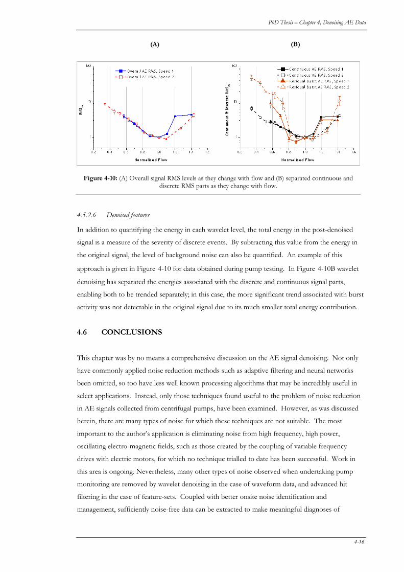
PhD Thesis – Chapter 4, Denoising AE Data
(A) (B)
Figure 4-10: (A) Overall signal RMS levels as they change with flow and (B) separated continuous and discrete RMS parts as they change with flow.
4.5.2.6 Denoised features
In addition to quantifying the energy in each wavelet level, the total energy in the post-denoised
signal is a measure of the severity of discrete events. By subtracting this value from the energy in
the original signal, the level of background noise can also be quantified. An example of this
approach is given in Figure 4-10 for data obtained during pump testing. In Figure 4-10B wavelet
denoising has separated the energies associated with the discrete and continuous signal parts,
enabling both to be trended separately; in this case, the more significant trend associated with burst
activity was not detectable in the original signal due to its much smaller total energy contribution.
4.6 CONCLUSIONS
This chapter was by no means a comprehensive discussion on the AE signal denoising. Not only
have commonly applied noise reduction methods such as adaptive filtering and neural networks
been omitted, so too have less well known processing algorithms that may be incredibly useful in
select applications. Instead, only those techniques found useful to the problem of noise reduction
in AE signals collected from centrifugal pumps, have been examined. However, as was discussed
herein, there are many types of noise for which these techniques are not suitable. The most
important to the author’s application is eliminating noise from high frequency, high power,
oscillating electro-magnetic fields, such as those created by the coupling of variable frequency
drives with electric motors, for which no technique trialled to date has been successful. Work in
this area is ongoing. Nevertheless, many other types of noise observed when undertaking pump
monitoring are removed by wavelet denoising in the case of waveform data, and advanced hit
filtering in the case of feature-sets. Coupled with better onsite noise identification and
management, sufficiently noise-free data can be extracted to make meaningful diagnoses of
4-16

PhD Thesis – Chapter 4, Denoising AE Data
conditions within centrifugal pumps. This will be the subject of further discussions in Chapters 8
and 9.
4-17

5. DDAATTAA
MMAANNAAGGEEMMEENNTT
Sikorska, J., Kelly, P. and Pan J.,
Mechanical Systems and Signal Processing,
(2005) In press.
55The aim of this chapter is to present a system that can administer and process, using techniques
discussed in previous chapters, an unlimited amount of AE data efficiently, effectively and with
rigorous quality assurance.
Publication Abstract
The use of acoustic emission testing in continuous monitoring applications presents the analyst
with the problem of managing substantial volumes of generated data. To better administer this
information, a system has been developed to catalogue, store and process AE data. Based on a
relational database, it is independent of the software and hardware used to acquire the data. This
paper describes the system and how it is used. Guidance is also given on how to optimise the
database for performance, robustness and ease of data extraction. Finally, examples of its data
mining capabilities are also presented.
5.1 INTRODUCTION
A data driven approach to signal processing involves cataloguing primary data according to a set of
descriptive parameters (known as meta- or tertiary data) and using these parameters to drive
automated, or semi-automated, signal processing and reporting. Results of processing generate
additional, derivative datasets (known as secondary data), which may also be stored and catalogued.
In the application presented here, acoustic emission (AE) hit information, waveform arrays and
time-logged parameters form the primary data, whilst statistics describing this primary data, such as
RMS, kurtosis and wavelet level energies, comprise the secondary data. Tertiary (meta-) data then
5-1
PhD Thesis, Chapter 5 – Data management
consists of information such as equipment TAG numbers, plant, channel information, dates and
operating conditions (flow, NPSH etc). Traditional file-based and data-driven management systems
are compared in Table 5-1.
The primary reason for the authors adopting a data driven methodology was the volume of
information generated by the application of AE to condition monitoring of rotating equipment; the
aim of which is to detect incipient, random failure of internal machinery components or the
damaging conditions that initiate failure. Whereas an AE structural test, conducted over a finite
time period, may result in a few thousand bursts and possibly 10’s of megabytes of waveform data,
a typical day’s continuous monitoring can produce between one hundred thousand and three
million AE events and around 2 gigabytes of waveform data. A single condition monitoring
session can last for days, weeks or months.
Dealing with data on this scale presents a number of challenges:
(1) Filing and retrieving data: Whilst it is feasible to have a folder on a computer file-system
containing several thousand files, few computers can present their users with a list of millions
of files in a timely and useful manner. Amongst other things, a file-system can only assign one,
meaningful attribute (the file name) to a piece of data. This is inadequate in a large-scale
system. Storing metadata in a searchable database provides a rich mechanism for identifying
and retrieving primary data, irrespective of whether the source file is stored on disk or archived
offline.
(2) Dealing consistently with data: In an application where collected data is to be post processed by an
evolving population of techniques, keeping track of what algorithms have been applied to what
datasets requires significant time and effort. By updating the metadata automatically as each
piece of primary data is analysed, an audit trail is created and the integrity of the analysis
assured.
(3) Modularity: Any attempt to analyse large amounts of data will, invariably, involve a mosaic of
techniques, often drawn from disparate applications or libraries. A data-driven approach, such
as the one presented here, provides a modular infrastructure into which post- processing
modules can be easily integrated and applied to sets of primary data. This facilitates direct
comparisons of techniques across statistically significant numbers of samples.
5-2
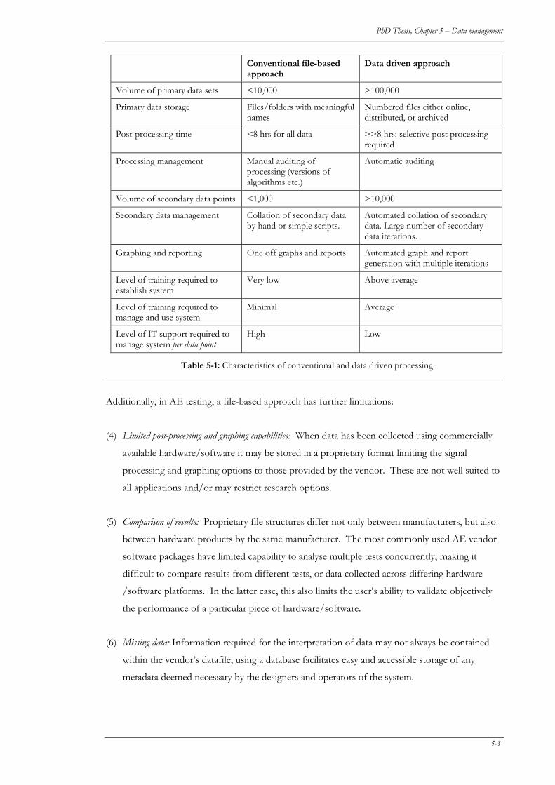
PhD Thesis, Chapter 5 – Data management
Conventional file-based approach
Data driven approach
Volume of primary data sets <10,000 >100,000
Primary data storage Files/folders with meaningful names
Numbered files either online, distributed, or archived
Post-processing time <8 hrs for all data >>8 hrs: selective post processing required
Processing management Manual auditing of processing (versions of algorithms etc.)
Automatic auditing
Volume of secondary data points <1,000 >10,000
Secondary data management Collation of secondary data by hand or simple scripts.
Automated collation of secondary data. Large number of secondary data iterations.
Graphing and reporting One off graphs and reports Automated graph and report generation with multiple iterations
Level of training required to establish system
Very low Above average
Level of training required to manage and use system
Minimal Average
Level of IT support required to manage system per data point
High Low
Table 5-1: Characteristics of conventional and data driven processing.
Additionally, in AE testing, a file-based approach has further limitations:
(4) Limited post-processing and graphing capabilities: When data has been collected using commercially
available hardware/software it may be stored in a proprietary format limiting the signal
processing and graphing options to those provided by the vendor. These are not well suited to
all applications and/or may restrict research options.
(5) Comparison of results: Proprietary file structures differ not only between manufacturers, but also
between hardware products by the same manufacturer. The most commonly used AE vendor
software packages have limited capability to analyse multiple tests concurrently, making it
difficult to compare results from different tests, or data collected across differing hardware
/software platforms. In the latter case, this also limits the user’s ability to validate objectively
the performance of a particular piece of hardware/software.
(6) Missing data: Information required for the interpretation of data may not always be contained
within the vendor’s datafile; using a database facilitates easy and accessible storage of any
metadata deemed necessary by the designers and operators of the system.
5-3
PhD Thesis, Chapter 5 – Data management
(7) Restrictions to accessing data: If data is collected using a commercially available software package,
analysing it on other machines may not be possible without purchasing additional licenses of
the software. This restricts data sharing and can represent a significant cost to the user.
An acoustic emission data management and analysis system (DBMAS), named ‘AEData’, was
developed to overcome these restrictions. Based on a Relational Database Management System
(RDBMS) implemented in Microsoft SQL Server, AEData catalogues all data files created by any
data acquisition system, extracts the data contained therein, co-ordinates batch post-processing
routines and collates the results of this post-processing, before arranging the results into a format
suitable for graphing.
Although some literature on the use of relational databases for managing condition monitoring data
has been published, the proposed models are primarily, either for storing and mining data [22, 23,
115], or as configuration management tools [129]. No reports have been found where these
systems are used to drive the analysis of data in a structured way. Commercial software packages
for administrating condition-monitoring data (eg. EXAKT, Ivara EXP, Avantis.CM) also use
relational databases, but these programs have their own in-built processing capabilities and tend not
to facilitate the addition of custom processing modules. Therefore, they do not offer the flexibility
required for research or development applications. Furthermore, commercial database
management systems are often prohibitively expensive.
5.2 DATABASE THEORY (PK)
A database is a file or a set of files in which information is stored. Within the file, data is grouped
in tables; each table holds a set rows; each row is a set of fields that collectively represent one
instance of that datum.
Rows in one table are usually related to rows in other tables either directly or transitively. These
relationships are implemented as part of the structure of the database and it is from them that the
term “Relational Database Management System” or RDBMS is derived. To appreciate the
difference between these types of relationships, consider the following scenario: waveform data
collected from a particular pump is stored in one table, details about the test in another table and
information about the pump (including its manufacturer) is contained in a third table.
Linguistically, the relationships between the data can be described as:
“These waveforms are from test A which used pump B from manufacturer C.”
5-4
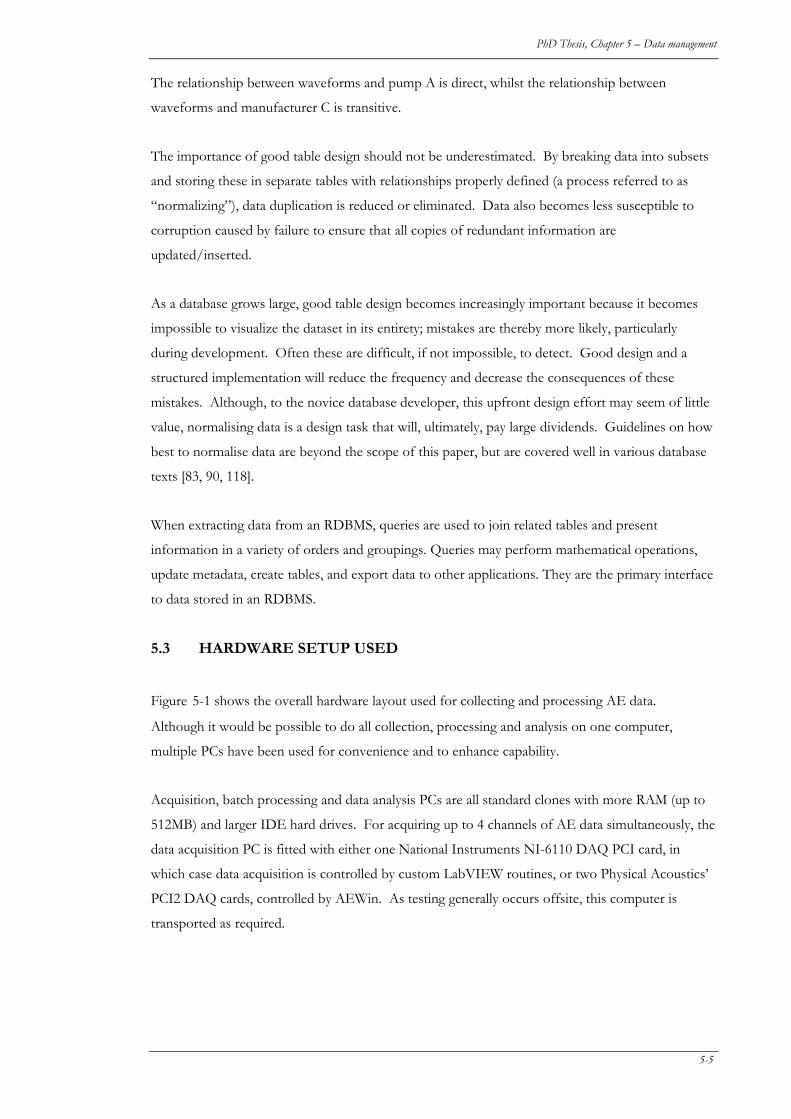
PhD Thesis, Chapter 5 – Data management
The relationship between waveforms and pump A is direct, whilst the relationship between
waveforms and manufacturer C is transitive.
The importance of good table design should not be underestimated. By breaking data into subsets
and storing these in separate tables with relationships properly defined (a process referred to as
“normalizing”), data duplication is reduced or eliminated. Data also becomes less susceptible to
corruption caused by failure to ensure that all copies of redundant information are
updated/inserted.
As a database grows large, good table design becomes increasingly important because it becomes
impossible to visualize the dataset in its entirety; mistakes are thereby more likely, particularly
during development. Often these are difficult, if not impossible, to detect. Good design and a
structured implementation will reduce the frequency and decrease the consequences of these
mistakes. Although, to the novice database developer, this upfront design effort may seem of little
value, normalising data is a design task that will, ultimately, pay large dividends. Guidelines on how
best to normalise data are beyond the scope of this paper, but are covered well in various database
texts [83, 90, 118].
When extracting data from an RDBMS, queries are used to join related tables and present
information in a variety of orders and groupings. Queries may perform mathematical operations,
update metadata, create tables, and export data to other applications. They are the primary interface
to data stored in an RDBMS.
5.3 HARDWARE SETUP USED
Figure 5-1 shows the overall hardware layout used for collecting and processing AE data.
Although it would be possible to do all collection, processing and analysis on one computer,
multiple PCs have been used for convenience and to enhance capability.
Acquisition, batch processing and data analysis PCs are all standard clones with more RAM (up to
512MB) and larger IDE hard drives. For acquiring up to 4 channels of AE data simultaneously, the
data acquisition PC is fitted with either one National Instruments NI-6110 DAQ PCI card, in
which case data acquisition is controlled by custom LabVIEW routines, or two Physical Acoustics’
PCI2 DAQ cards, controlled by AEWin. As testing generally occurs offsite, this computer is
transported as required.
5-5
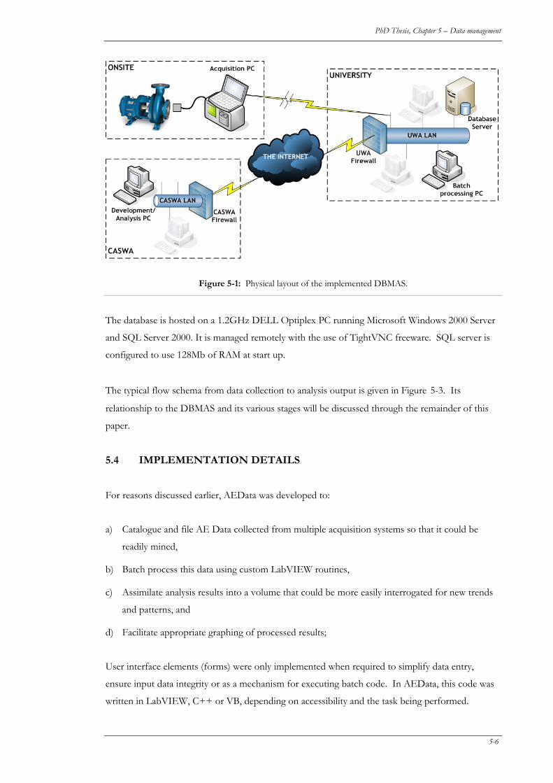
PhD Thesis, Chapter 5 – Data management
Figure 5-1: Physical layout of the implemented DBMAS.
The database is hosted on a 1.2GHz DELL Optiplex PC running Microsoft Windows 2000 Server
and SQL Server 2000. It is managed remotely with the use of TightVNC freeware. SQL server is
configured to use 128Mb of RAM at start up.
The typical flow schema from data collection to analysis output is given in Figure 5-3. Its
relationship to the DBMAS and its various stages will be discussed through the remainder of this
paper.
5.4 IMPLEMENTATION DETAILS
For reasons discussed earlier, AEData was developed to:
a) Catalogue and file AE Data collected from multiple acquisition systems so that it could be
readily mined,
b) Batch process this data using custom LabVIEW routines,
c) Assimilate analysis results into a volume that could be more easily interrogated for new trends
and patterns, and
d) Facilitate appropriate graphing of processed results;
User interface elements (forms) were only implemented when required to simplify data entry,
ensure input data integrity or as a mechanism for executing batch code. In AEData, this code was
written in LabVIEW, C++ or VB, depending on accessibility and the task being performed.
5-6
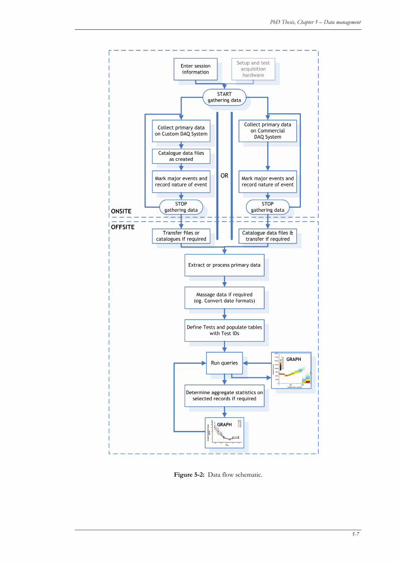
PhD Thesis, Chapter 5 – Data management
Figure 5-2: Data flow schematic.
5-7
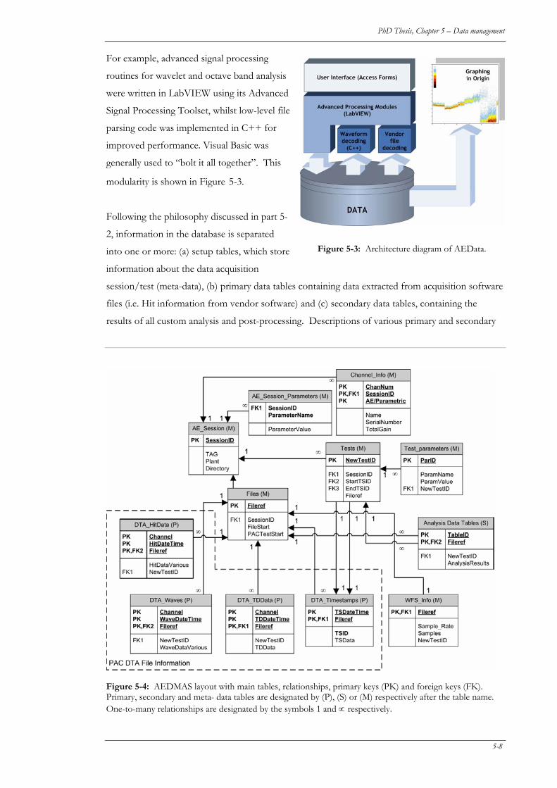
PhD Thesis, Chapter 5 – Data management
For example, advanced signal processing
routines for wavelet and octave band analysis
were written in LabVIEW using its Advanced
Signal Processing Toolset, whilst low-level file
parsing code was implemented in C++ for
improved performance. Visual Basic was
generally used to “bolt it all together”. This
modularity is shown in Figure 5-3.
Following the philosophy discussed in part 5-
2, information in the database is separated
into one or more: (a) setup tables, which store
information about the data acquisition
session/test (meta-data), (b) primary data tables containing data extracted from acquisition software
files (i.e. Hit information from vendor software) and (c) secondary data tables, containing the
results of all custom analysis and post-processing. Descriptions of various primary and secondary
Figure 5-3: Architecture diagram of AEData.
Figure 5-4: AEDMAS layout with main tables, relationships, primary keys (PK) and foreign keys (FK). Primary, secondary and meta- data tables are designated by (P), (S) or (M) respectively after the table name. One-to-many relationships are designated by the symbols 1 and ∝ respectively.
5-8
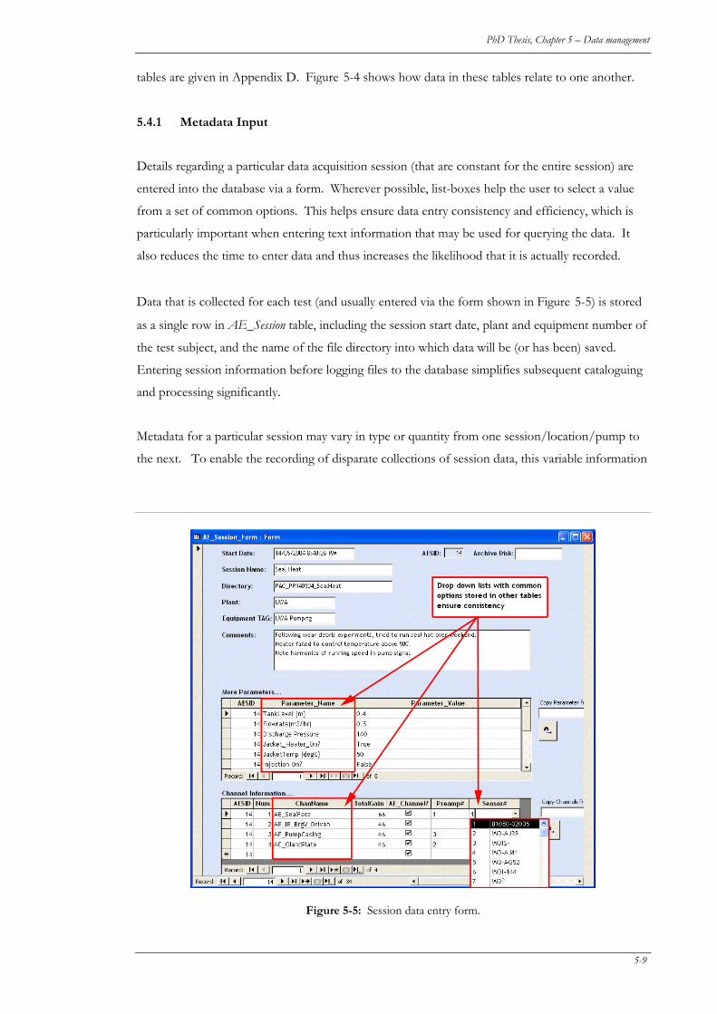
PhD Thesis, Chapter 5 – Data management
tables are given in Appendix D. Figure 5-4 shows how data in these tables relate to one another.
5.4.1 Metadata Input
Details regarding a particular data acquisition session (that are constant for the entire session) are
entered into the database via a form. Wherever possible, list-boxes help the user to select a value
from a set of common options. This helps ensure data entry consistency and efficiency, which is
particularly important when entering text information that may be used for querying the data. It
also reduces the time to enter data and thus increases the likelihood that it is actually recorded.
Data that is collected for each test (and usually entered via the form shown in Figure 5-5) is stored
as a single row in AE_Session table, including the session start date, plant and equipment number of
the test subject, and the name of the file directory into which data will be (or has been) saved.
Entering session information before logging files to the database simplifies subsequent cataloguing
and processing significantly.
Metadata for a particular session may vary in type or quantity from one session/location/pump to
the next. To enable the recording of disparate collections of session data, this variable information
Figure 5-5: Session data entry form.
5-9

PhD Thesis, Chapter 5 – Data management
is saved to a separate table (AE_Session_Parameters). Here the value of each piece of data
(ParameterValue) is stored along with its associated parameter name (ParameterName) as separate
rows. There is no limit to the number of parameters that can be recorded about a particular
session. Channel information (name, number, gain, type, sensor serial number etc) about either
AE or Parametric (non-AE) channels is stored in a third table, again as separate rows, facilitating
cataloguing of details from any number of channels (AE or parametric) per session. If the
acquisition computer is not connected to the database, session data (and associated channels and
parameters) are stored locally and synchronised later.
Once a session has ended and the primary data collected, another form is used to upload and
catalogue all files in the database. This form initiates routines that copy all filenames for one or
more acquisition sessions, along with their type and creation date to the Files table. Data can also
be transferred from one hard-drive to another, which is useful when separate PCs collect and
process the data. With custom written data acquisition software, logging file information can be
performed at the time of data capture (although data transfer is still initiated later). Using
commercial software this is rarely possible and filenames must be copied separately. The
implementation of this process ensures that all files collected are catalogued and accounted for. In
an environment where a session may produce more than 10,000 files it can be difficult to obtain
this level of rigorous quality assurance manually.
Figure 5-6: Process Files Form extracts information from DTA files and analyses WFS files.
5-10
PhD Thesis, Chapter 5 – Data management
5.4.2 Primary data input
Once AE data files have been catalogued and filed by the system, any data contained therein can be
extracted or processed. Again, a form (Figure 5-6) is used to drive this process. Visual Basic code
associated with the ‘GO’ button calls LabVIEW routines that have been compiled into a dynamic
link library, to perform file parsing and data extraction. Separate routines are implemented for
each file type. For example, a processing library was created in LabVIEW to read DTA files
created by AEWin for Physical Acoustics’ PCI2 data acquisition hardware. This code extracts: (a)
information about the acquisition setup (HDT, HLT, whether it is a new file or a continuation of a
previous file etc), (b) hit features, (c) time-dependant AE and parametric data, and (d) timestamps,
as well as any metadata not recorded elsewhere. Each data group is saved in a separate table for
reasons discussed previously.
The location of any burst waveforms within the DTA file and information required to interpret
them is determined and stored. This includes the waveform channel, number of samples, sampling
rate and total gain, which facilitates very quick data mining for waveforms thereafter (eg. when
averaging waveforms and/or determining continuous wavelet transforms). It should be noted that
Visual Basic, Matlab or a C variant could have be used as an alternative to LabVIEW and may be
judged by some to be more appropriate. Irrespective of the language used for file parsing, this
task’s level of complexity depends on the accuracy of documentation provided by the supplier of
the acquisition code. Unfortunately, this may not always be complete or accurate. If the originator
is unwilling or unable to provide this information, reverse engineering of file formats may be
required using low-level tools (eg. a Hex Editor) and a good deal of patience.
5.4.3 Secondary data input
One of the requirements for the database was to enable waveform-streaming files (typically
containing unscaled waveforms between 1 and 2 million samples long) to be subjected to advanced
and automated signal analysis. Accordingly, LabVIEW/C++ routines were developed to read,
scale and process the files using wavelet and spectral functions supplied with the LabVIEW Signal
Processing Toolbox (version 2). These programs were then compiled into libraries that could be
invoked by the batch processing routines within AEData. The results of each processing method
are stored in separate tables, with links to the originating file record. (In the context of this
DBMAS, the raw waveforms represent primary data, albeit they are not stored in the database,
whilst the analysis results are the secondary data.)
Figure 5-6 shows the batch processing control screen. A user selects a session in the list box, along
with the types of analysis/post-processing required. The database identifies the files from the tests
5-11
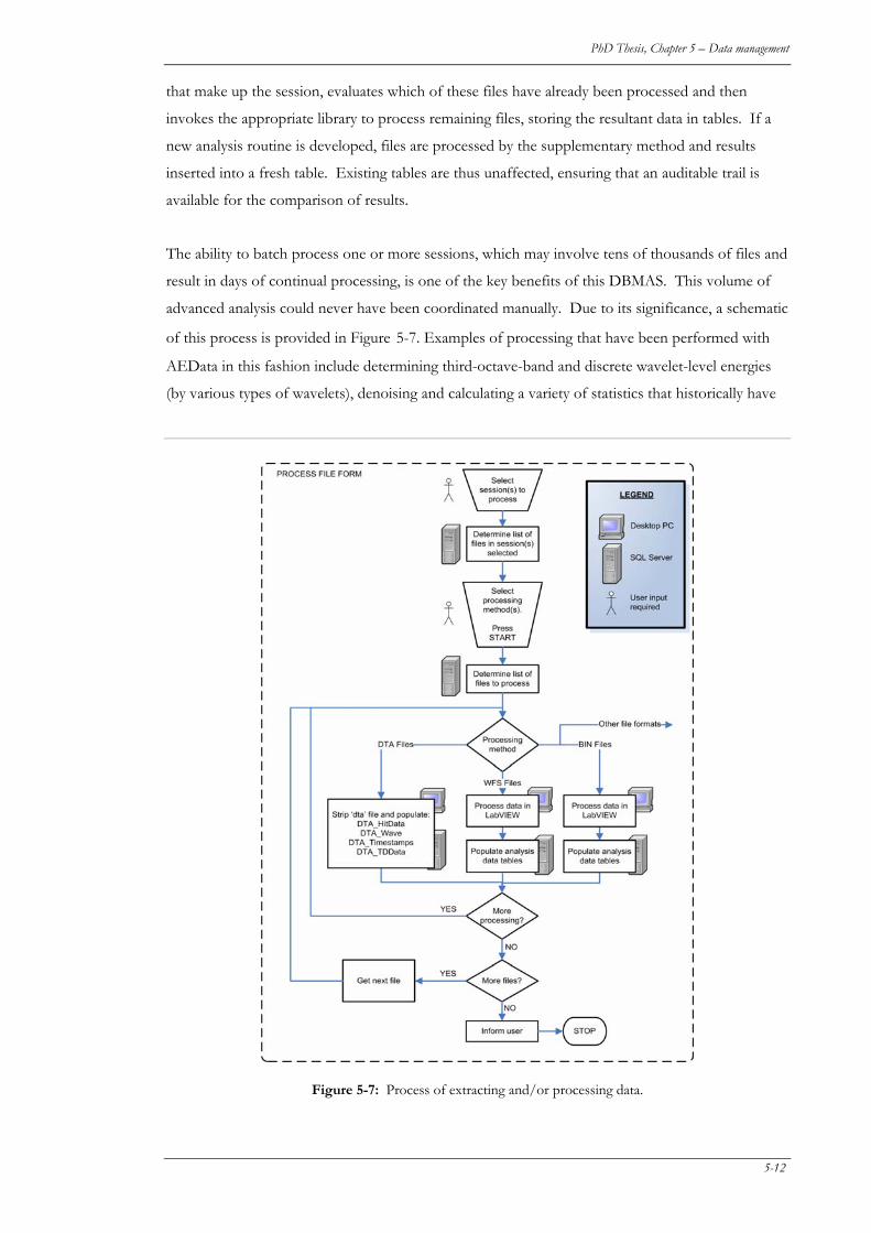
PhD Thesis, Chapter 5 – Data management
that make up the session, evaluates which of these files have already been processed and then
invokes the appropriate library to process remaining files, storing the resultant data in tables. If a
new analysis routine is developed, files are processed by the supplementary method and results
inserted into a fresh table. Existing tables are thus unaffected, ensuring that an auditable trail is
available for the comparison of results.
The ability to batch process one or more sessions, which may involve tens of thousands of files and
result in days of continual processing, is one of the key benefits of this DBMAS. This volume of
advanced analysis could never have been coordinated manually. Due to its significance, a schematic
of this process is provided in Figure 5-7. Examples of processing that have been performed with
AEData in this fashion include determining third-octave-band and discrete wavelet-level energies
(by various types of wavelets), denoising and calculating a variety of statistics that historically have
Figure 5-7: Process of extracting and/or processing data.
5-12
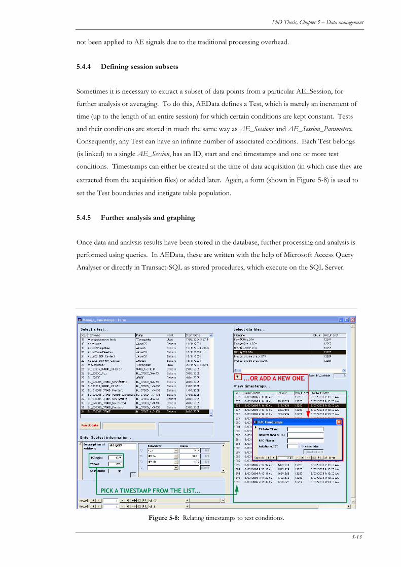
PhD Thesis, Chapter 5 – Data management
not been applied to AE signals due to the traditional processing overhead.
5.4.4 Defining session subsets
Sometimes it is necessary to extract a subset of data points from a particular AE_Session, for
further analysis or averaging. To do this, AEData defines a Test, which is merely an increment of
time (up to the length of an entire session) for which certain conditions are kept constant. Tests
and their conditions are stored in much the same way as AE_Sessions and AE_Session_Parameters.
Consequently, any Test can have an infinite number of associated conditions. Each Test belongs
(is linked) to a single AE_Session, has an ID, start and end timestamps and one or more test
conditions. Timestamps can either be created at the time of data acquisition (in which case they are
extracted from the acquisition files) or added later. Again, a form (shown in Figure 5-8) is used to
set the Test boundaries and instigate table population.
5.4.5 Further analysis and graphing
Once data and analysis results have been stored in the database, further processing and analysis is
performed using queries. In AEData, these are written with the help of Microsoft Access Query
Analyser or directly in Transact-SQL as stored procedures, which execute on the SQL Server.
Figure 5-8: Relating timestamps to test conditions.
5-13
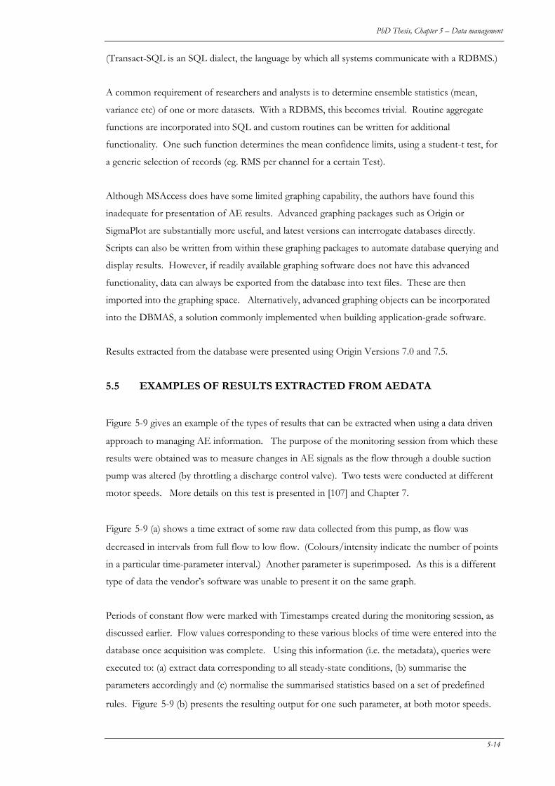
PhD Thesis, Chapter 5 – Data management
(Transact-SQL is an SQL dialect, the language by which all systems communicate with a RDBMS.)
A common requirement of researchers and analysts is to determine ensemble statistics (mean,
variance etc) of one or more datasets. With a RDBMS, this becomes trivial. Routine aggregate
functions are incorporated into SQL and custom routines can be written for additional
functionality. One such function determines the mean confidence limits, using a student-t test, for
a generic selection of records (eg. RMS per channel for a certain Test).
Although MSAccess does have some limited graphing capability, the authors have found this
inadequate for presentation of AE results. Advanced graphing packages such as Origin or
SigmaPlot are substantially more useful, and latest versions can interrogate databases directly.
Scripts can also be written from within these graphing packages to automate database querying and
display results. However, if readily available graphing software does not have this advanced
functionality, data can always be exported from the database into text files. These are then
imported into the graphing space. Alternatively, advanced graphing objects can be incorporated
into the DBMAS, a solution commonly implemented when building application-grade software.
Results extracted from the database were presented using Origin Versions 7.0 and 7.5.
5.5 EXAMPLES OF RESULTS EXTRACTED FROM AEDATA
Figure 5-9 gives an example of the types of results that can be extracted when using a data driven
approach to managing AE information. The purpose of the monitoring session from which these
results were obtained was to measure changes in AE signals as the flow through a double suction
pump was altered (by throttling a discharge control valve). Two tests were conducted at different
motor speeds. More details on this test is presented in [107] and Chapter 7.
Figure 5-9 (a) shows a time extract of some raw data collected from this pump, as flow was
decreased in intervals from full flow to low flow. (Colours/intensity indicate the number of points
in a particular time-parameter interval.) Another parameter is superimposed. As this is a different
type of data the vendor’s software was unable to present it on the same graph.
Periods of constant flow were marked with Timestamps created during the monitoring session, as
discussed earlier. Flow values corresponding to these various blocks of time were entered into the
database once acquisition was complete. Using this information (i.e. the metadata), queries were
executed to: (a) extract data corresponding to all steady-state conditions, (b) summarise the
parameters accordingly and (c) normalise the summarised statistics based on a set of predefined
rules. Figure 5-9 (b) presents the resulting output for one such parameter, at both motor speeds.
5-14
PhD Thesis, Chapter 5 – Data management
(A) (B)
Figure 5-9: Raw AE data and corresponding secondary data obtained for a pump flow test.
5.6 OPTIMISING PERFORMANCE (PK)
5.6.1 Hardware
The speed of an RDBMS is only a second order function of CPU speed, so upgrading the CPU will
only provide a marginal improvement in database performance. Other techniques are therefore
required to promote efficient interaction when databases increase in size or complexity.
As tables become large, queries that involve joins will begin to slow. Initially, and intuitively, this
will correlate with an increase in CPU utilization on the database server. There will come a point
however, where a step increase in processing time is observed, coinciding with a step decrease in
CPU utilization. This happens because the storage space required for the temporary table created
by a join is larger than the amount of RAM available to the RDBMS. Consequently, the RDBMS
builds the temporary table on disk rather than in memory. Accessing information on a computer
hard-drive is two orders of magnitude slower than accessing information stored in RAM; hence the
server reports 100% disk utilization and a low CPU load. This phenomenon is referred to as
bottlenecking. The system, in the described state, would be “disk bound” and this is why
production, multi-user database servers have several gigabytes of memory installed.
If a dedicated computer is to be used for the RDBMS then it is recommended that consideration be
given to providing it with as much memory and as fast hard disks as budget permits. Adding an
additional 1-2GB of memory will deliver a profound increase in performance. Furthermore, if the
database is to be hosted on a centrally managed server, data and processing requirements should be
5-15
PhD Thesis, Chapter 5 – Data management
reviewed periodically with the database administrator so that the system can be tuned and
appropriate times chosen to run batch-processing jobs.
The RDBMS component of AEData was originally installed on a server with 256MB of memory
and a standard hard drive. Performance was adequate until one or more tables started exceeding a
couple of million records. At this point it became necessary to upgrade the amount of RAM and
install a RAID disk controller.
5.6.2 Indexes
The most significant improvement in data processing speed comes from the creation and
management of indexes. Indexes increase performance because the RDBMS will endeavour to
store the associated data in RAM rather than on disk. A table may have several indexes defined.
To create an index, a subset of fields within a table (that can be used to select and sort records from
that table) is nominated. Some database tools will analyse a query and make recommendations
about indexing which can be useful for novice database developers.
In AEData indexes generally included table ID fields (SessionID, TestID, Fileref etc) and
Channel_number. Additionally, fields commonly used for generating queries (parameter_name,
test_description) were also defined as Indexes.
5.6.3 Stored Procedures
Stored procedures are scripts that run on the database server. They are usually written in a version
of SQL. Where bulk updates of data are needed, these scripts generally run about twice as fast as
the equivalent code implemented in a client based application such as MSAccess. This occurs
because there is no overhead of client/server communication. It also reduces load on the network
significantly.
5.7 CONCLUSIONS
Although the system described was developed for use on AE data collected from rotating
machinery, it is equally applicable to any other type of AE testing. In fact, the general approach is
relevant to any signal source that results in large volumes of data requiring storage, processing
and/or data mining. From a design perspective, a data-driven management system such as this has
no inherent functional limitations on number of channels, tests or post-processing routines. The
number of concurrent users depends primarily on the database management software. If budget
5-16
PhD Thesis, Chapter 5 – Data management
constraints dictate, it can be (and has been) implemented on relatively inexpensive desktop
hardware, albeit configured appropriately.
The biggest advantage of this approach however, is that millions of data points can be analysed as
desired, with auditable rigour, and minimal manual intervention. Also crucially important, accessing
and mining the data, is simplified greatly because it is now independent of both the hardware and
software that was used for its creation/acquisition. This frees the analyst or researcher to process
and graph their data as required, instead of being hampered by the limitations of vendor software.
Once primary data has been extracted from data acquisition files, or analysis routines performed on
raw waveform data, files can be archived, reducing storage overheads associated with massive
amounts of raw data. Collating results in one place also simplifies the process of backing up and
archiving. Research effort and time can then be spent developing and assessing new signal
processing techniques on statistically significant sample sizes, rather than simply administrating the
information.
5.8 POSTSCRIPT
The database management system described in this chapter was fundamental to all work
subsequently described in this thesis. Processing modules were written (primarily by the author) in
Visual Basic, TransactSQL or LabVIEW for all techniques described in chapters 3 and 4. Queries
were developed (by the author or Mr Kelly) to extract subsets of these processed results for
ensemble averaging and/or plotting in Origin. Even graphs of individual waveform files used the
database management system to locate desired files. Although resulting images were not stored or
catalogued in the database, this would be an obvious extension to the current system and may be
incorporated into future versions.
5-17
6. EEFFFFEECCTT OOFF WWAAVVEEGGUUIIDDEESS
-- PPAARRTT OONNEE
Sikorska, J. and Pan, J.,
Journal of Acoustic Emission,
2004, Vol 22, pp. 264-273.
66The aims of this chapter are to:
(a) Identify how waveguides affect the transmission of simulated acoustic emission signals to
the sensor;
(b) Illustrate some of the issues relating to AE signal transmission that can complicate AE data
analysis.
Publication Abstract
This paper presents the effects of varying waveguide material and/or shape on traditional acoustic
emission characteristics of pulsed events. Forty-eight solid cylindrical waveguides were fabricated
from either alumina ceramic, mild steel, stainless steel (SS316), 2024-T3 aluminium or extruded
Delrin. Three different lengths, two diameters and four sensor face angles were tested. The effects
of a point contact at the source end of the waveguide were also verified. Results show that
although ceramic guides attenuate the signals more than commonly used grades of steel and
aluminium, waveform fidelity is less affected. Point contacts at the source end also had a negative
effect on all AE features and waveform profiles.
Equation Chapter 6 Section 1
6-1
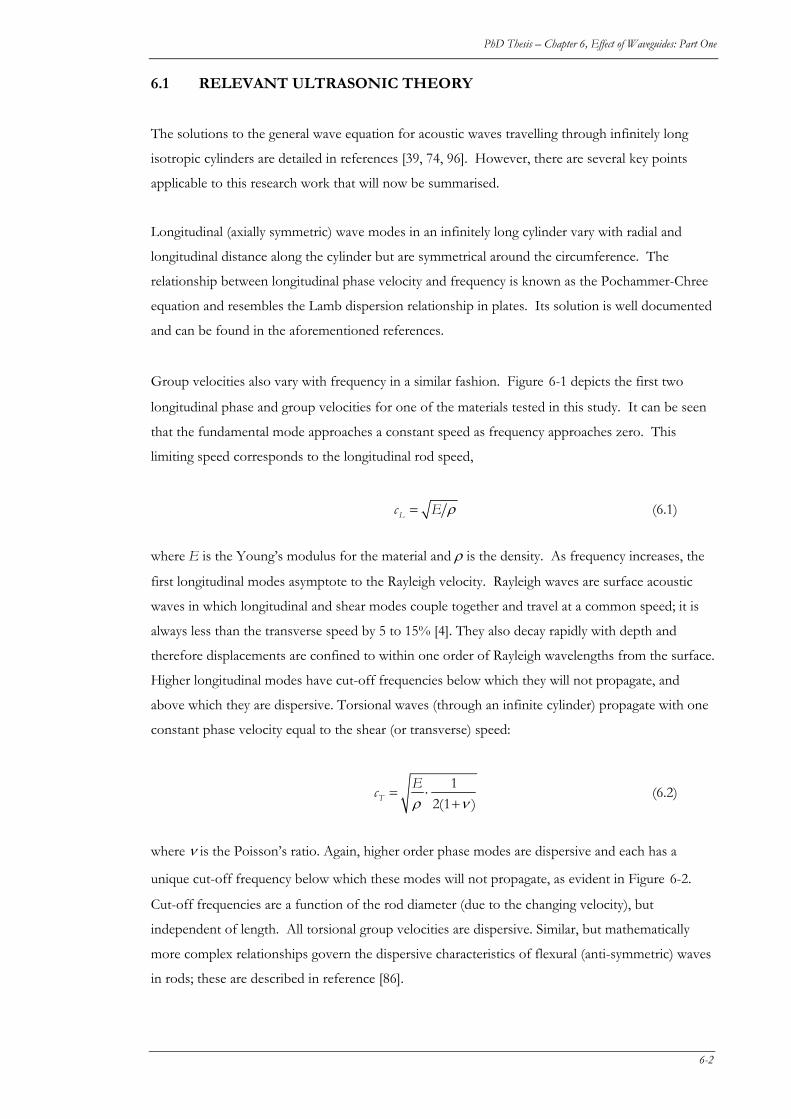
PhD Thesis – Chapter 6, Effect of Waveguides: Part One
6.1 RELEVANT ULTRASONIC THEORY
The solutions to the general wave equation for acoustic waves travelling through infinitely long
isotropic cylinders are detailed in references [39, 74, 96]. However, there are several key points
applicable to this research work that will now be summarised.
Longitudinal (axially symmetric) wave modes in an infinitely long cylinder vary with radial and
longitudinal distance along the cylinder but are symmetrical around the circumference. The
relationship between longitudinal phase velocity and frequency is known as the Pochammer-Chree
equation and resembles the Lamb dispersion relationship in plates. Its solution is well documented
and can be found in the aforementioned references.
Group velocities also vary with frequency in a similar fashion. Figure 6-1 depicts the first two
longitudinal phase and group velocities for one of the materials tested in this study. It can be seen
that the fundamental mode approaches a constant speed as frequency approaches zero. This
limiting speed corresponds to the longitudinal rod speed,
Lc E ρ= (6.1)
where E is the Young’s modulus for the material and ρ is the density. As frequency increases, the
first longitudinal modes asymptote to the Rayleigh velocity. Rayleigh waves are surface acoustic
waves in which longitudinal and shear modes couple together and travel at a common speed; it is
always less than the transverse speed by 5 to 15% [4]. They also decay rapidly with depth and
therefore displacements are confined to within one order of Rayleigh wavelengths from the surface.
Higher longitudinal modes have cut-off frequencies below which they will not propagate, and
above which they are dispersive. Torsional waves (through an infinite cylinder) propagate with one
constant phase velocity equal to the shear (or transverse) speed:
1E2(1 )Tc ρ ν
= ⋅+
(6.2)
where ν is the Poisson’s ratio. Again, higher order phase modes are dispersive and each has a
unique cut-off frequency below which these modes will not propagate, as evident in Figure 6-2.
Cut-off frequencies are a function of the rod diameter (due to the changing velocity), but
independent of length. All torsional group velocities are dispersive. Similar, but mathematically
more complex relationships govern the dispersive characteristics of flexural (anti-symmetric) waves
in rods; these are described in reference [86].
6-2

PhD Thesis – Chapter 6, Effect of Waveguides: Part One
At very narrow diameters, cut-off effects act like a high pass filter, leaving only lower order modes
as the means by which low frequency longitudinal, torsional and flexural waves can be transmitted.
Conversely, above a certain frequency, which is a function of rod diameter and material properties
(namely E, ρ, and ν) speeds approach their limiting values and dispersion will no longer occur. In
this interim region however, where wavelength is in the same order as the rod diameter, significant
dispersive effects can be expected.
In addition to dispersion, AE bursts are attenuated as they travel through the material. Some of
this energy loss is caused by friction and thermal conductivity and occurs in all materials,
independent of frequency. However in compounds with larger grain sizes, such as plastics or
composites, frequency-dependant attenuation can increase significantly (by up to 3 orders of
magnitude) when compared to metals. Attenuation is also generally greater for transverse waves
than for longitudinal modes. Finally, it is important to recognise that AE sensors are not equally
sensitive to all wave modes, causing further apparent signal reduction of various modes.
One side effect of dispersion is the tendency of AE bursts, which are made up of numerous waves
of different polarizations and consequently different speeds, to lengthen in time as they move
further from the source. Called mode separation, continuous transformation between modes
exacerbates this effect [26].
In a finite rod, wave motion becomes even more complicated due to reflections from, and
resonance at, both ends [85]. Acoustic waves are partially reflected and transmitted at every
interface, the relative amounts of which depend on the ratio of the relative characteristic
impedances of each pair of boundary materials. This impedance is a function of material density
and the speed of the wave hitting the interface. If material attenuation is low, these reflections will
combine with late arriving components of the original signal, thus complicating feature
identification.
For non-zero angles of incidence, the character of the wavefront will also change as it hits the
interface. Called mode conversion, the change in angle of the wavefront will convert part of the
incoming wave from longitudinal to shear and vice versa. Flexural waves that may not have been
present in the original waveform can also be excited.
Finally, cylinders have natural frequencies that are a function of their length and wave velocity. As
an AE burst is made up of numerous waves of different frequencies, resonance can be expected.
Another interesting effect of dispersion is that higher order resonant modes are no longer integer
multiples of the fundamental frequency. This can complicate identification of these artefacts.
6-3

PhD Thesis – Chapter 6, Effect of Waveguides: Part One
In traditional AE processing, various AE features are used for describing AE signals, as described
in previous chapters. Amplitude and frequency analysis are more meaningful features for measuring
continuous emissions, whilst count rate and energy analysis are useful for burst emission
characterisation [95]. Defining a burst as an event that exceeds a certain threshold, the following
features will be extracted and analysed in Part 1 of this study:
• Peak amplitude
• Burst energy
• Duration and/or total counts
• Rise time and/or counts to peak
• Signal strength.
6.2 EXPERIMENTAL METHOD
A variety of short waveguides were tested to illustrate the effects of: (a) material properties; (b)
length; (c) diameter; (d) face angle and (e) source point on the transmission and reception of pulsed
AE bursts.
Forty-eight (48) waveguides were tested in total, fabricated from five materials: Delrin acetal resin
(white extruded bar, exact grade unknown), common mild steel (exact grade unknown), SS316,
2024-T3 aluminium and sintered 99.9% alumina ceramic (α-Al2O3). Approximate material
properties are summarised in Table 6-1. Sensor face angles were 0˚, 30˚, 45˚ or 60˚; lengths were
30, 43 or 51 mm; and diameters were 5 or 8 mm. Unless otherwise stated, the rod face attached to
the pulser was flat.
Test specimens were grouped as follows:
(a) 5 sets of 8-mm diameter waveguides with face angles of 0˚, 30˚, 45˚ and 60˚ from each
of the four materials (20 waveguides in total). Lengths were set at 43 mm between
centres (at which pulser and receiver were located). (Four sets shown Figure 6-3A.)
(b) 3 sets of 8-mm diameter, shorter (30 mm) waveguides with face angles of 0˚, 30˚, 45˚
and 60˚; from Delrin, 2024-T3 aluminium and SS316.
(c) 2 sets of narrower (5 mm) mild steel rods, 30mm and 43mm in length, with face angles
of 0˚, 30˚, 45˚ and 60˚.
6-4
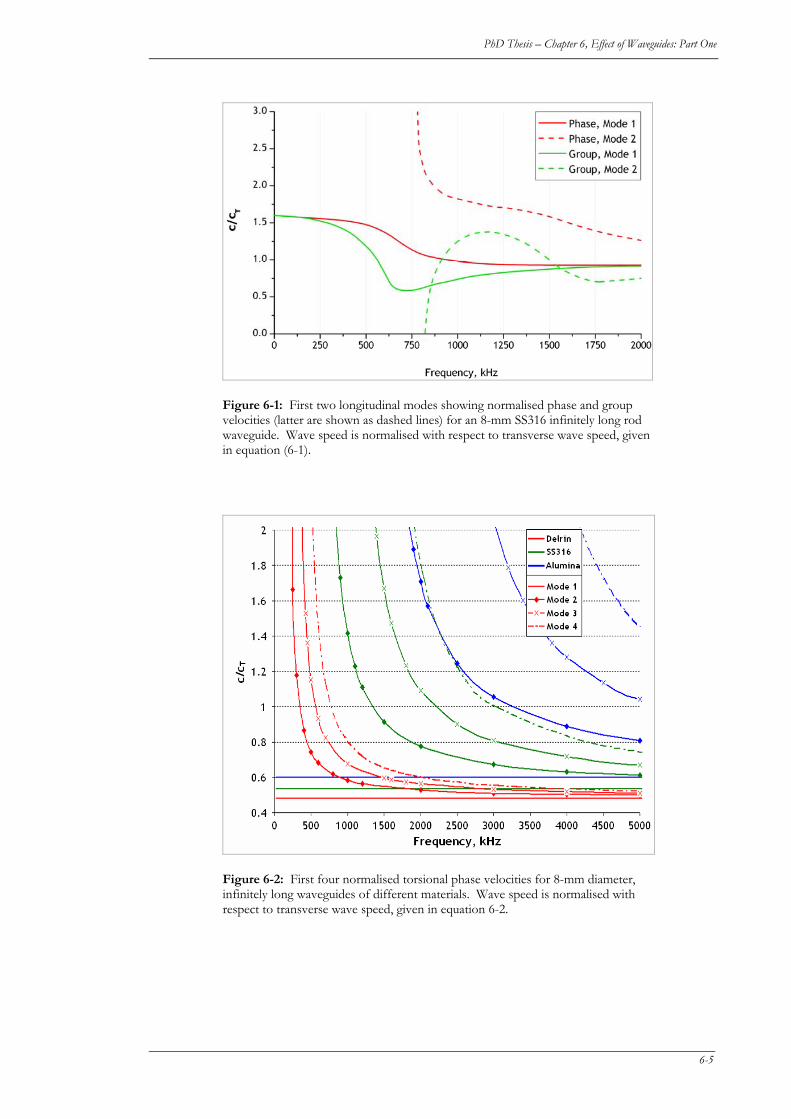
PhD Thesis – Chapter 6, Effect of Waveguides: Part One
Figure 6-1: First two longitudinal modes showing normalised phase and group velocities (latter are shown as dashed lines) for an 8-mm SS316 infinitely long rod waveguide. Wave speed is normalised with respect to transverse wave speed, given in equation (6-1).
Figure 6-2: First four normalised torsional phase velocities for 8-mm diameter, infinitely long waveguides of different materials. Wave speed is normalised with respect to transverse wave speed, given in equation 6-2.
6-5
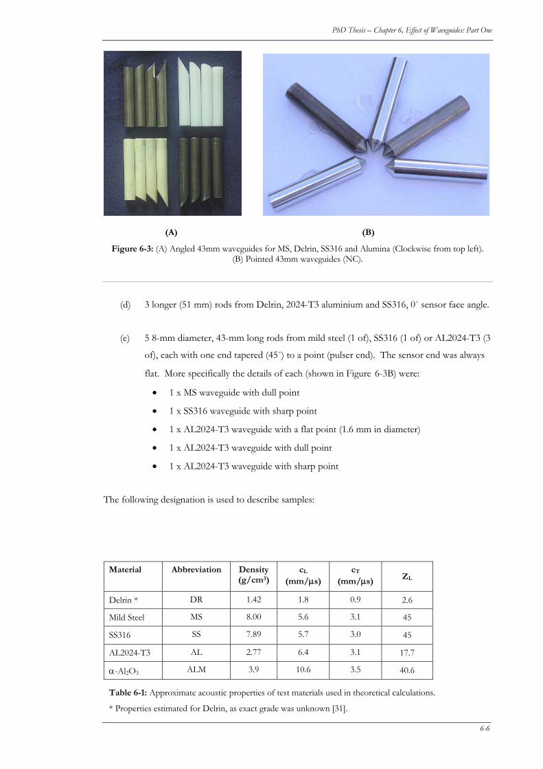
PhD Thesis – Chapter 6, Effect of Waveguides: Part One
(A) (B)
Figure 6-3: (A) Angled 43mm waveguides for MS, Delrin, SS316 and Alumina (Clockwise from top left). (B) Pointed 43mm waveguides (NC).
(d) 3 longer (51 mm) rods from Delrin, 2024-T3 aluminium and SS316, 0˚ sensor face angle.
(e) 5 8-mm diameter, 43-mm long rods from mild steel (1 of), SS316 (1 of) or AL2024-T3 (3
of), each with one end tapered (45˚) to a point (pulser end). The sensor end was always
flat. More specifically the details of each (shown in Figure 6-3B) were:
• 1 x MS waveguide with dull point
• 1 x SS316 waveguide with sharp point
• 1 x AL2024-T3 waveguide with a flat point (1.6 mm in diameter)
• 1 x AL2024-T3 waveguide with dull point
• 1 x AL2024-T3 waveguide with sharp point
The following designation is used to describe samples:
Material Abbreviation Density (g/cm3)
cL (mm/μs)
cT (mm/μs) ZL
DR 1.42 1.8 0.9 Delrin * 2.6
Mild Steel MS 8.00 5.6 3.1 45
SS316 SS 7.89 5.7 3.0 45
AL2024-T3 AL 2.77 6.4 3.1 17.7
ALM 3.9 10.6 3.5 40.6 α-Al2O3
Table 6-1: Approximate acoustic properties of test materials used in theoretical calculations.
* Properties estimated for Delrin, as exact grade was unknown [31].
6-6
PhD Thesis – Chapter 6, Effect of Waveguides: Part One
Material x OD in mm x Length in mm “PT” (optional).
6-7

PhD Thesis – Chapter 6, Effect of Waveguides: Part One
To quantify the effect of each waveguide, data
was also collected from the sensor mounted
directly on the pulser face. The resulting
values were used to normalise all data.
Longitudinal pulses, representative of AE
bursts, were generated by a DECI Model
SE25-P sensor driven by a DECI Model 600
pulser, set at 150V5. A waveguide holder
(Figure 6-4) was fabricated to ensure that the
relative positions of the sensor, waveguide and
pulser were kept constant (Figure 6-5). The
pulser was attached to the underside of the
holder with a Delrin collar containing 8 rare
earth magnets and two locating pins to ensure
repeatable orientation. Incorporated into the
sensor mount was a screw and spring that held
the sensor firmly against the top waveguide
face. This could be oriented to any angle.
O-rings prevented the waveguides from contacting the sides of the sample holder. Silicone grease
was used as a couplant between the pulser-waveguide and waveguide-sensor faces.
Figure 6-4: Waveguide holder.
Bursts were detected using a B1080 Digital Wave Corp. single-ended wideband AE sensor
connected to a PAC 2/4/6 preamplifier supplying a gain of 20 dB and fitted with 100-1000 kHz
bandpass filters. Data was recorded by a PAC PCI-2 card, housed in a 2.8-GHz Pentium-IV
desktop computer. Prior to digitisation, signals were bandpass filtered onboard at 1-3000 kHz. A
fixed trigger threshold was set at 50 dBAE. For each waveguide, between 128 and 300 triggered
waveforms, each consisting of 8192 samples with 256 pre-trigger samples, were collected and
digitised at 10 MHz.
Various burst features were collected using AEWin software for each triggered event, including
peak amplitude (in dBAE), AE energy, signal strength, duration, rise time and AE counts. These
5 Locating the pulser at the geometric centre of the waveguide avoided the excitation of torsional or
flexural waves. (NC)
6-8
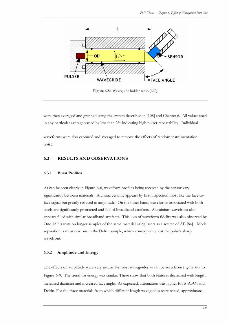
PhD Thesis – Chapter 6, Effect of Waveguides: Part One
Figure 6-5: Waveguide holder setup (NC).
were then averaged and graphed using the system described in [108] and Chapter 6. All values used
in any particular average varied by less than 2% indicating high pulser repeatability. Individual
waveforms were also captured and averaged to remove the effects of random instrumentation
noise.
6.3 RESULTS AND OBSERVATIONS
6.3.1 Burst Profiles
As can be seen clearly in Figure 6-6, waveform profiles being received by the sensor vary
significantly between materials. Alumina ceramic appears by first inspection most like the face-to-
face signal but greatly reduced in amplitude. On the other hand, waveforms associated with both
steels are significantly protracted and full of broadband artefacts. Aluminium wavefront also
appears filled with similar broadband artefacts. This loss of waveform fidelity was also observed by
Ono, in his tests on longer samples of the same material using lasers as a source of AE [84]. Mode
separation is most obvious in the Delrin sample, which consequently lost the pulse’s sharp
wavefront.
6.3.2 Amplitude and Energy
The effects on amplitude were very similar for most waveguides as can be seen from Figure 6-7 to
Figure 6-9. The trend for energy was similar. These show that both features decreased with length,
increased diameter and increased face angle. As expected, attenuation was higher for α-Al2O3 and
Delrin. For the three materials from which different length waveguides were tested, approximate
6-9
PhD Thesis – Chapter 6, Effect of Waveguides: Part One
values for attenuation were calculated (see Table 6-2). Although these numbers are very
approximate, they do indicate that Delrin’s broadband attenuation is highly non-linear and in this
application (across the frequency range studied) significantly less than predicted by the literature.
6-10
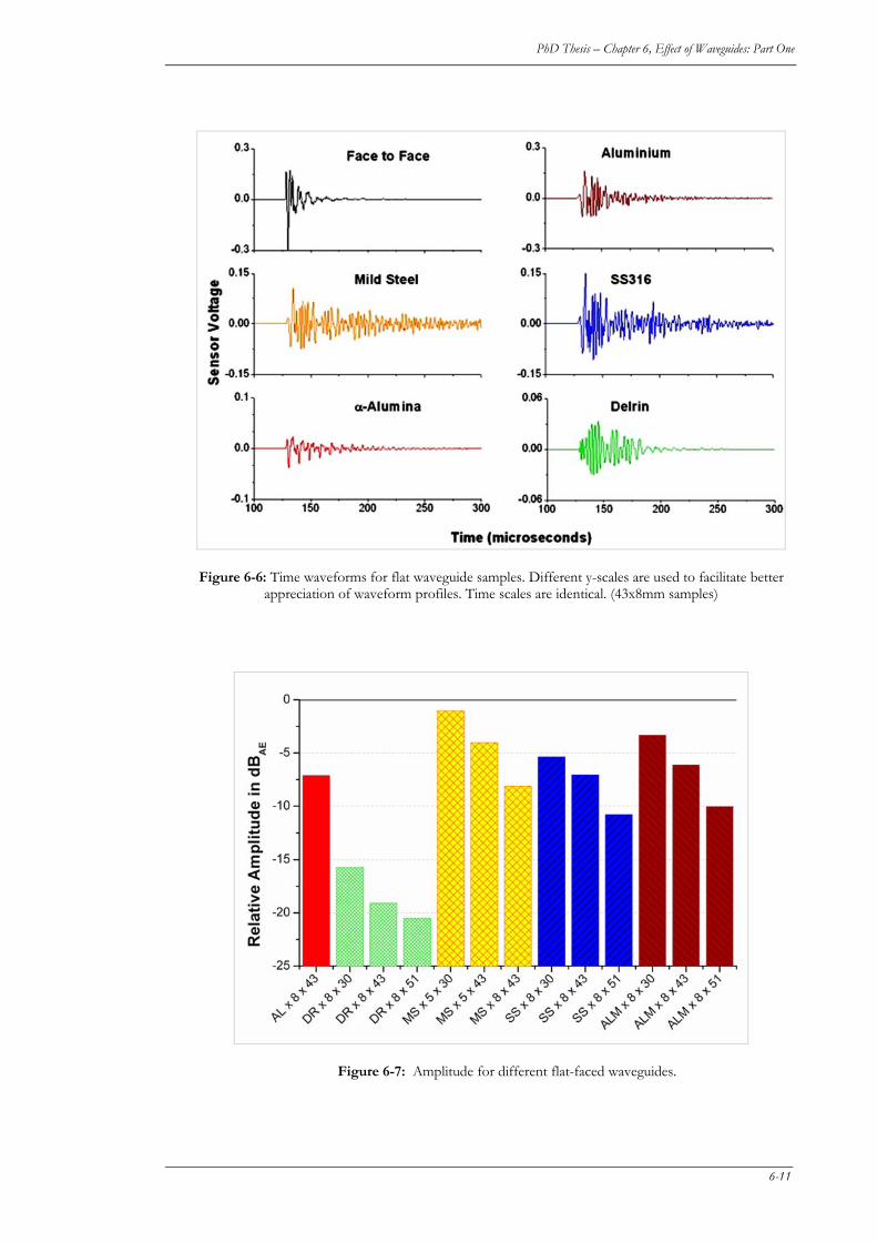
PhD Thesis – Chapter 6, Effect of Waveguides: Part One
Figure 6-6: Time waveforms for flat waveguide samples. Different y-scales are used to facilitate better appreciation of waveform profiles. Time scales are identical. (43x8mm samples)
Figure 6-7: Amplitude for different flat-faced waveguides.
6-11
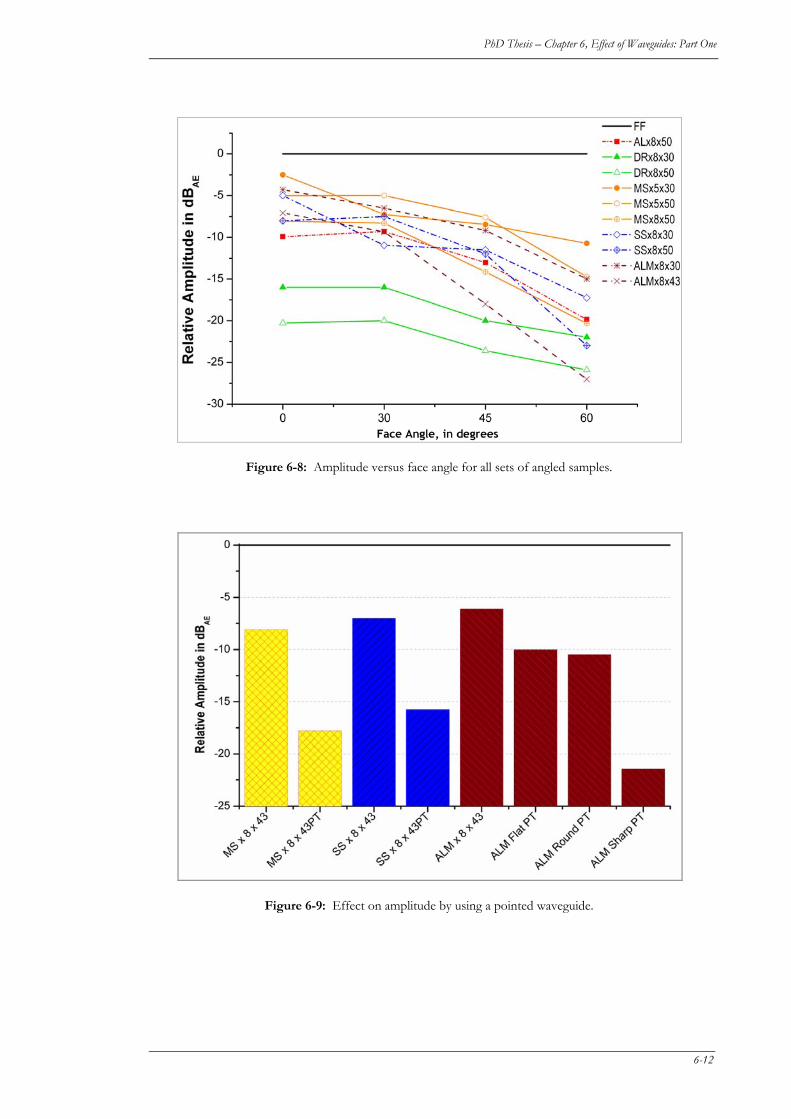
PhD Thesis – Chapter 6, Effect of Waveguides: Part One
Figure 6-8: Amplitude versus face angle for all sets of angled samples.
Figure 6-9: Effect on amplitude by using a pointed waveguide.
6-12
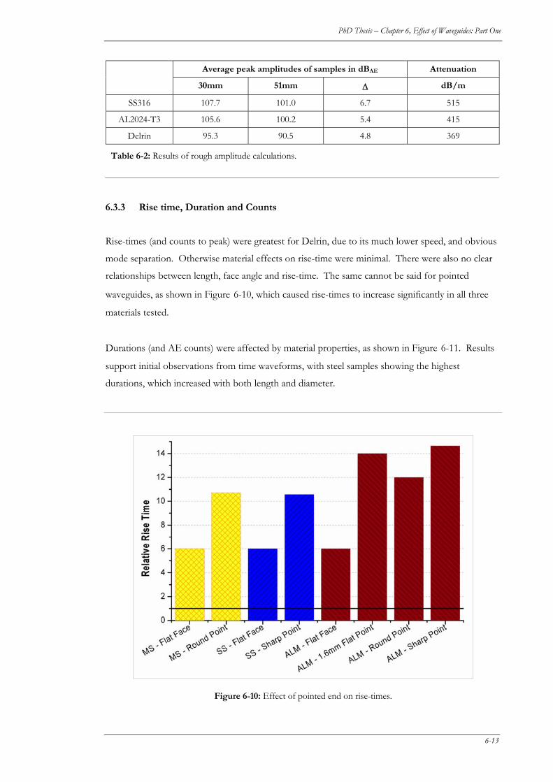
PhD Thesis – Chapter 6, Effect of Waveguides: Part One
6.3.3 Rise time, Duration and Counts
Rise-times (and counts to peak) were greatest for Delrin, due to its much lower speed, and obvious
mode separation. Otherwise material effects on rise-time were minimal. There were also no clear
relationships between length, face angle and rise-time. The same cannot be said for pointed
waveguides, as shown in Figure 6-10, which caused rise-times to increase significantly in all three
materials tested.
Durations (and AE counts) were affected by material properties, as shown in Figure 6-11. Results
support initial observations from time waveforms, with steel samples showing the highest
durations, which increased with both length and diameter.
Figure 6-10: Effect of pointed end on rise-times.
Average peak amplitudes of samples in dBAE Attenuation
30mm 51mm Δ dB/m
SS316 107.7 101.0 6.7 515
AL2024-T3 105.6 100.2 5.4 415
Delrin 95.3 90.5 4.8 369
Table 6-2: Results of rough amplitude calculations.
6-13
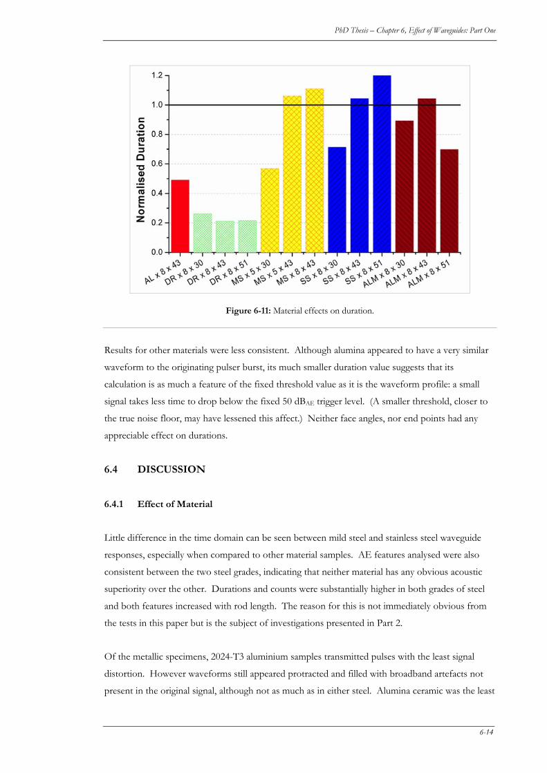
PhD Thesis – Chapter 6, Effect of Waveguides: Part One
Figure 6-11: Material effects on duration.
Results for other materials were less consistent. Although alumina appeared to have a very similar
waveform to the originating pulser burst, its much smaller duration value suggests that its
calculation is as much a feature of the fixed threshold value as it is the waveform profile: a small
signal takes less time to drop below the fixed 50 dBAE trigger level. (A smaller threshold, closer to
the true noise floor, may have lessened this affect.) Neither face angles, nor end points had any
appreciable effect on durations.
6.4 DISCUSSION
6.4.1 Effect of Material
Little difference in the time domain can be seen between mild steel and stainless steel waveguide
responses, especially when compared to other material samples. AE features analysed were also
consistent between the two steel grades, indicating that neither material has any obvious acoustic
superiority over the other. Durations and counts were substantially higher in both grades of steel
and both features increased with rod length. The reason for this is not immediately obvious from
the tests in this paper but is the subject of investigations presented in Part 2.
Of the metallic specimens, 2024-T3 aluminium samples transmitted pulses with the least signal
distortion. However waveforms still appeared protracted and filled with broadband artefacts not
present in the original signal, although not as much as in either steel. Alumina ceramic was the least
6-14
PhD Thesis – Chapter 6, Effect of Waveguides: Part One
distorted of all materials, with signals appearing similar to the originating bursts. Delrin, due to its
much slower wave speed, showed the clearest mode separation of all materials.
As predicted, overall attenuation of both energy and peak amplitude was greatest in non-metallic
waveguides, however rudimentary calculations based on drop in peak amplitude for different
lengths indicated that this was not as severe as was expected. Furthermore, any attenuation present
in Delrin seemed to be non-linear and therefore longer waveguides caused proportionally less
attenuation than shorter guides across the traditional AE bandwidth.
6.4.2 Effect of Length, Diameter and Face angle
Attenuation also increased with length and diameter (where measured). Reasons for the latter are
not clear, and were only tested for one material (mild steel) but may be due to the increased number
of modes present in wider rods (below cut-off). This will be discussed further in Part 2. In all
materials, attenuation increased significantly with face angle, particularly above 30 degrees. This is
probably because mode conversion is causing redirection of energy into modes that the transducer
is less able to detect.
6.4.3 Effect of Pointed Source End
Pointed 43-mm waveguides attenuated the signals by over 12 dB when compared to similar flat
waveguides with adequate couplant. This was greater than the attenuation quoted by other
researchers [84, 128]. The type of point also made a significant difference on amplitude and energy
attenuation with finer (sharper) points causing greater signal reduction than rounder or flat points.
This may explain the discrepancy between these values and those published in other work.
6.5 CONCLUSIONS
Although signals passing through metallic waveguides were not attenuated significantly, signals
were protracted and appeared as if contaminated by reflections and resonance artefacts. Conditions
deteriorated with length and diameter. It is possible that much longer waveguides (>100mm) might
avoid this problem due to the additional attenuation that would be incurred; however this requires
further investigation. On the other hand, α-Al2O3 did not suffer from this problem, with primary
bursts being easily separated from subsequent reflections. Although alumina had a higher overall
attenuation, measured bursts showed significantly less distortion and (except for amplitude and
energy due to its increased attenuation) best-matched AE features of face-to-face signals.
6-15
PhD Thesis – Chapter 6, Effect of Waveguides: Part One
Unfortunately, use of waveguides in AE testing cannot be avoided, however their implementation
must be properly considered. Whenever feasible, specific designs should be tested prior to
installation to determine actual transmission characteristics.
Further effects on transmission of frequency and modal information were investigated in reference
[110], which has been included as the next chapter of this thesis.
6-16
7. EEFFFFEECCTT OOFF WWAAVVEEGGUUIIDDEESS
-- PPAARRTT TTWWOO
Sikorska, J. and Pan, J.,
Journal of Acoustic Emission, 2004,
Vol 22, pp. 274-287.
77 The aims of this chapter are to:
(a) Identify how waveguides affect the transmission of frequency information corresponding
to simulated acoustic emission signals to the sensor;
(b) Illustrate some of the issues relating to AE signal transmission that can complicate AE data
analysis.
Equation Chapter 7 Section 1
Publication Abstract
This paper presents the effects of varying waveguide material and/or shape on the frequency and
joint-time-frequency characteristics of pulsed acoustic emission (AE) events. Forty-eight solid
cylindrical waveguides were fabricated from either alumina ceramic, mild steel, stainless steel
(SS316), 2024-T3 aluminium or extruded Delrin. Three different lengths, two diameters and four
sensor face angles were tested. The effects of a point at the source end of the waveguide were also
verified. Analysis methods included continuous wavelets, short time Fourier transforms and
standard Fourier transforms. Results show that detected signals were dominated by the resonant
harmonics of the waveguides, particularly with commonly used waveguide materials such as
aluminium and steel.
7-1
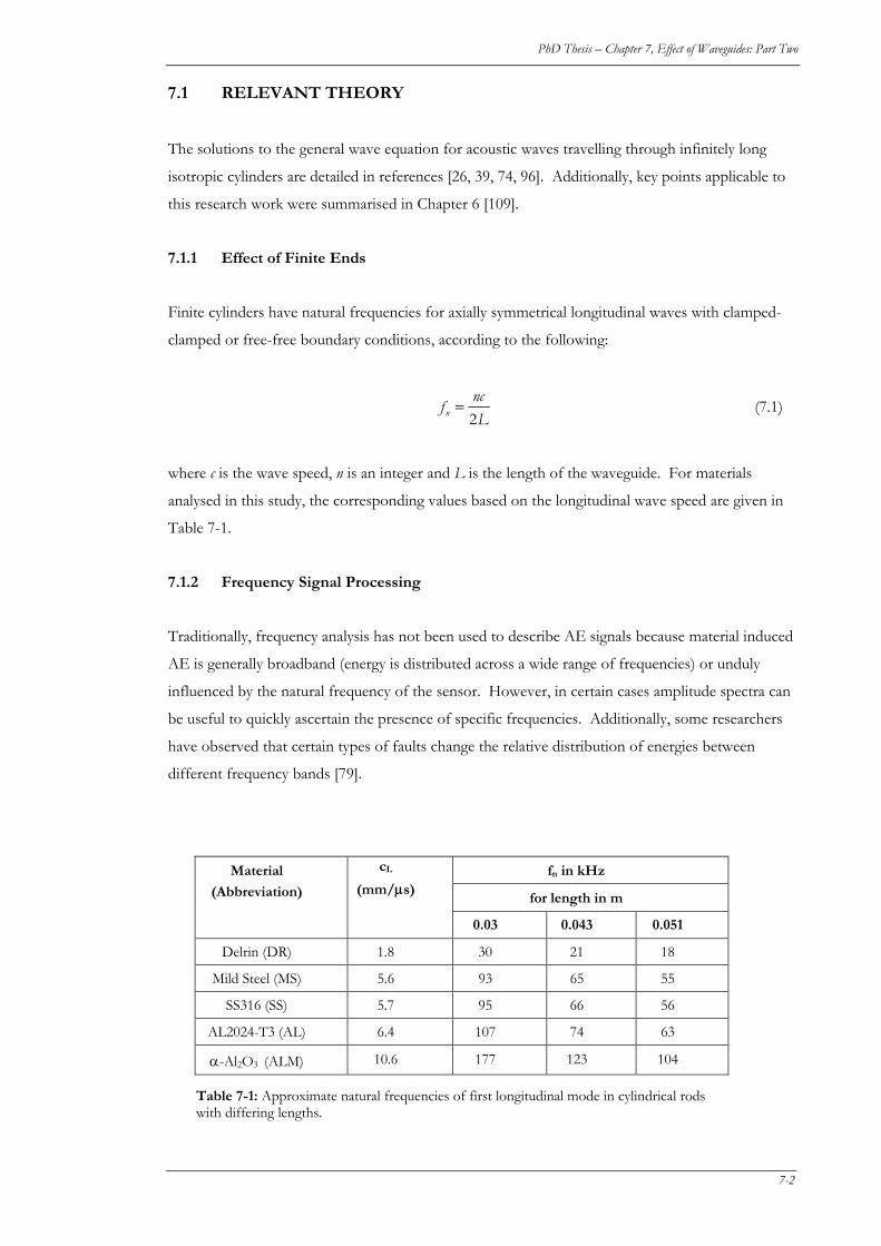
PhD Thesis – Chapter 7, Effect of Waveguides: Part Two
7.1 RELEVANT THEORY
The solutions to the general wave equation for acoustic waves travelling through infinitely long
isotropic cylinders are detailed in references [26, 39, 74, 96]. Additionally, key points applicable to
this research work were summarised in Chapter 6 [109].
7.1.1 Effect of Finite Ends
Finite cylinders have natural frequencies for axially symmetrical longitudinal waves with clamped-
clamped or free-free boundary conditions, according to the following:
2nncfL
= (7.1)
where c is the wave speed, n is an integer and L is the length of the waveguide. For materials
analysed in this study, the corresponding values based on the longitudinal wave speed are given in
Table 7-1.
7.1.2 Frequency Signal Processing
Traditionally, frequency analysis has not been used to describe AE signals because material induced
AE is generally broadband (energy is distributed across a wide range of frequencies) or unduly
influenced by the natural frequency of the sensor. However, in certain cases amplitude spectra can
be useful to quickly ascertain the presence of specific frequencies. Additionally, some researchers
have observed that certain types of faults change the relative distribution of energies between
different frequency bands [79].
fn in kHz cL Material
for length in m (mm/μs) (Abbreviation)
0.03 0.043 0.051
Delrin (DR) 1.8 30 21 18
Mild Steel (MS) 5.6 93 65 55
SS316 (SS) 5.7 95 66 56
AL2024-T3 (AL) 6.4 107 74 63
10.6 177 123 104 α-Al2O3 (ALM)
Table 7-1: Approximate natural frequencies of first longitudinal mode in cylindrical rods with differing lengths.
7-2
PhD Thesis – Chapter 7, Effect of Waveguides: Part Two
7.1.3 Advanced Joint-Time-Frequency Techniques
Two frequently applied joint-time frequency techniques are Short Time Fourier Transforms (STFT)
and wavelets. These were introduced in Section 3.2.6.
The most commonly used wavelet in AE analysis is the Gabor (otherwise known as Morlet)
function [43], also used by the AGU-Vallen freeware. Its function is defined by the following:
(7.2) 2( ) exp( /2)cos(5 )w t t t= −
The relationship between scale, a, and centre frequency, fc, for the Morlet wavelet is given by the
following [91]:
52
s
c s
f where af f a>0
aπ
⎧⎪= ⎨⎪⎩
=0 (7.3)
where fs is the sampling rate in Hertz. The relationship between centre frequency and bandwidth
therefore becomes:
5 /2 5 0.81/ 2s sf a fcentre frequency
bandwidth aπ
π= = ≈ (7.4)
Similarly, the translated position on the x-axis, b, is determined by:
xb
s
b Nx where b=0,1,2...,N/Nf x
×= (7.5)
where Nx is the number of time samples per time division and N is the total number of samples.
For efficient computation, these should both be integral powers of 2 (eg. 64, 1024, 8192 etc).
7.1.4 Modal AE
It is assumed that specific faults propagate by a defined set of one or more dispersive modes, the
characteristics of which are a function of material properties and dimensions [109]. Modal AE
involves acquiring and digitizing AE time signals, from which individual propagation modes are
then identified and extracted. Information about particular modes can then be quantified in an
attempt to identify and/or source the underlying faults.
7-3
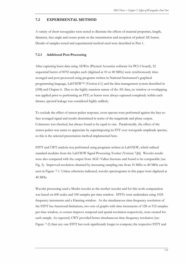
PhD Thesis – Chapter 7, Effect of Waveguides: Part Two
7.2 EXPERIMENTAL METHOD
A variety of short waveguides were tested to illustrate the effects of material properties, length,
diameter, face angle and source point on the transmission and reception of pulsed AE bursts.
Details of samples tested and experimental method used were described in Part 1.
7.2.1 Additional Post-Processing
After capturing burst data using AEWin (Physical Acoustics software for PCI-2 board), 32
sequential bursts of 8192 samples each (digitised at 10 or 40 MHz) were synchronously time-
averaged and post-processed using programs written in National Instrument’s graphical
programming language, LabVIEWTM (Version 6.1) and the data management system described in
[108] and Chapter 6. Due to the highly transient nature of the AE data, no window or overlapping
was applied prior to performing an FFT; as bursts were always captured completely within each
dataset, spectral leakage was considered highly unlikely.
To exclude the effect of sensor-pulser response, cross-spectra were performed against the face-to-
face averaged signal and results determined in terms of the magnitude and phase output.
Coherence was checked, but always found to be equal to one. Paradoxically, the effect of the
sensor-pulser was easier to appreciate by superimposing its FFT over waveguide amplitude spectra,
so this is the selected presentation method implemented here.
STFT and CWT analysis was performed using programs written in LabVIEW, which utilised
standard modules from the LabVIEW Signal Processing Toolset (Version 7)[6]. Wavelet results
were also compared with the output from AGU-Vallen freeware and found to be comparable (see
Fig. 3). Improved resolution obtained by increasing sampling rate from 10 MHz to 40 MHz can be
seen in Figure 7-1. Unless otherwise indicated, wavelet spectrograms in this paper were digitized at
40 MHz.
Wavelet processing used a Morlet wavelet as the mother wavelet and for this work computation
was based on 600 scales and 100 samples per time window. STFTs were undertaken using 1024
frequency increments and a Hanning window. As the simultaneous time-frequency resolution of
the STFT has functional limitations, two sets of graphs with time increments of 128 or 512 samples
per time window, to extract improve temporal and spatial resolution respectively, were created for
each sample. As expected, CWT provided better simultaneous time-frequency resolution (see
Figure 7-2) than any one STFT but took significantly longer to compute; the respective STFT and
7-4

PhD Thesis – Chapter 7, Effect of Waveguides: Part Two
CWT functions behind the spectrograms shown in Figure 7-2 took 594 and 15141 ms to calculate
respectively (i.e. wavelets took almost 30 times longer). Nevertheless, wavelets offer a visually more
7-5
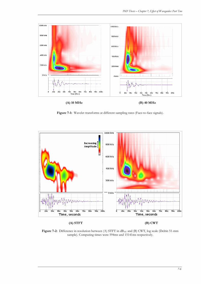
PhD Thesis – Chapter 7, Effect of Waveguides: Part Two
(A) 10 MHz (B) 40 MHz
Figure 7-1: Wavelet transforms at different sampling rates (Face-to-face signals).
(A) STFT (B) CWT
Figure 7-2: Difference in resolution between (A) STFT in dBAE and (B) CWT, log scale (Delrin 51-mm sample). Computing times were 594ms and 15141ms respectively.
7-6
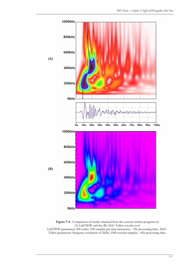
PhD Thesis – Chapter 7, Effect of Waveguides: Part Two
(A)
(B)
Figure 7-3: Comparison of results obtained from the custom written programs in (A) LabVIEW and the (B) AGU-Vallen wavelet tool.
LabVIEW parameters: 600 scales, 100 samples per time increment, ~30s processing time. AGU-Vallen parameters: frequency resolution of 5kHz, 1000 wavelet samples, ~60s processing time.
7-7
PhD Thesis – Chapter 7, Effect of Waveguides: Part Two
economic display of time-frequency information and therefore are predominantly shown herein. It
should be noted however, that computing multiple STFTs, with different time and frequency
intervals provides the same information in a much shorter time (albeit in two graphs), and therefore
would be more appropriate for real-time feature extraction.6
7.2.2 Modal Analysis
A commercially available software package called DISPERSE (Version 2.0.16c)7 was used to
generate individual modes for the materials being analysed. These were then superimposed over
the signals using a standard drawing package; frequency and time scales were matched
appropriately.
Unfortunately, exact material properties for the various materials (particularly Delrin and mild steel)
were not known and due to limited access to DISPERSE, examining slightly different values to
obtain better modal matching was not possible. Therefore some discrepancies can be expected,
particularly for Delrin and mild steel.
7.3 FREQUENCY RESULTS
7.3.1 Flat Waveguides
Resulting averaged amplitude spectra for all flat 43-mm waveguides are given in Figure 7-4. The
face-to-face spectrum is also plotted to show the effect of its non-uniform frequency response on
other results. (Wavelet plots are given in Figure 7-12.) Spectra of metallic waveguides are
dominated by harmonics of longitudinal rod frequencies. The first of these peaks (~60 kHz)
matches the results listed in Table 7-2. This is confirmed by observing the changing location of
these peaks for different rod lengths (see Figure 7-5).
Alumina is also affected by rod resonance, but due to its much higher wave speed, there are fewer
harmonics permeating the bandwidth of interest. Additionally, the material’s frequency-dependant
damping seems to reduce the effect of rod resonance above 600 kHz. Similarly, Delrin’s high
damping [109] is probably the reason no resonant effects can be seen in its amplitude spectra.
6 This may also be a function of the algorithms used by National Instruments, Signal Processing Toolset for
LabVIEW. (NC)
7 Propagation modes using DISPERSE were determined by Dr. Mike Lowe from the NDT Lab at Imperial College in
London . (NC)
7-8
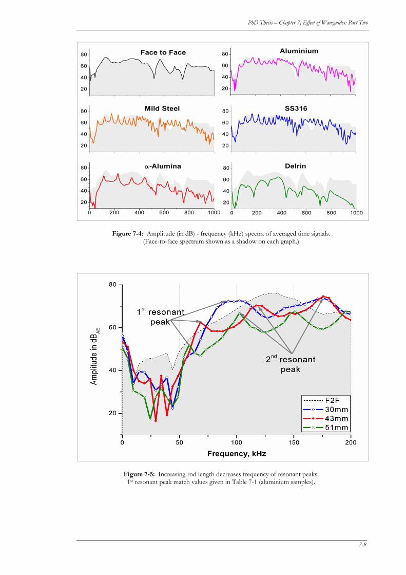
PhD Thesis – Chapter 7, Effect of Waveguides: Part Two
Figure 7-4: Amplitude (in dB) - frequency (kHz) spectra of averaged time signals. (Face-to-face spectrum shown as a shadow on each graph.)
Figure 7-5: Increasing rod length decreases frequency of resonant peaks. 1st resonant peak match values given in Table 7-1 (aluminium samples).
7-9
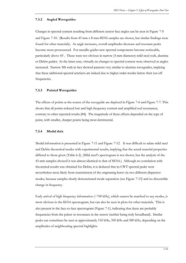
PhD Thesis – Chapter 7, Effect of Waveguides: Part Two
7.3.2 Angled Waveguides
Changes in spectral content resulting from different sensor face angles can be seen in Figure 7-9
and Figure 7-10. (Results from 43 mm x 8 mm SS316 samples are shown, but similar findings were
found for other materials). As angle increases, overall amplitudes decrease and resonant peaks
become more pronounced. For metallic guides new spectral components become noticeable,
particularly above 45˚. These were not obvious in narrow (5-mm diameter) mild steel rods, alumina
or Delrin guides. In the latter case, virtually no changes to spectral content were observed as angles
increased. Narrow MS rods in fact showed patterns very similar to alumina waveguides, implying
that these additional spectral artefacts are indeed due to higher order modes below their cut-off
frequencies.
7.3.3 Pointed Waveguides
The effects of points at the source of the waveguide are depicted in Figure 7-6 and Figure 7-7. This
shows that all points reduced low and high frequency content and amplified rod resonances,
contrary to other reported results [84]. The magnitude of these effects depended on the type of
point, with smaller, sharper points being most detrimental.
7.3.4 Modal data
Modal information is presented in Figure 7-11 and Figure 7-12. It was difficult to relate mild steel
and Delrin theoretical modes with experimental results, implying that the actual material properties
differed to those given (Table 6-2). (Mild steel’s spectrogram is not shown, but the analysis of the
43-mm samples showed it was almost identical to that of SS316.) Although no correlation with
theoretical results was obtained for Delrin, it is deduced that its CWT spectral peaks were
nevertheless most likely from transmission of the originating burst via two different dispersive
modes, because samples clearly demonstrated mode separation (see Figure 7-13) and no discernible
change in frequency.
Early arrival of high frequency information (~700 kHz), which cannot be matched to any modes, is
most obvious in the SS316 spectrogram, but can also be seen in plots for other materials. This is
also present in the face-to-face spectrogram (Figure 7-1), indicating that these are probably
frequencies from the pulser or resonance in the sensor (neither being truly broadband). Similar
peaks can sometimes be seen at approximately 110 kHz, 350 kHz and 580 kHz, depending on the
amplitudes of neighbouring spectral highlights.
7-10
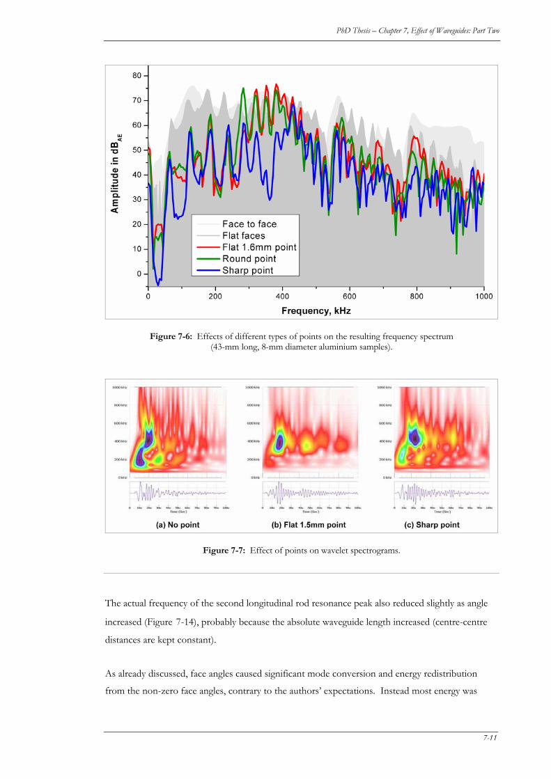
PhD Thesis – Chapter 7, Effect of Waveguides: Part Two
Figure 7-6: Effects of different types of points on the resulting frequency spectrum (43-mm long, 8-mm diameter aluminium samples).
Figure 7-7: Effect of points on wavelet spectrograms.
The actual frequency of the second longitudinal rod resonance peak also reduced slightly as angle
increased (Figure 7-14), probably because the absolute waveguide length increased (centre-centre
distances are kept constant).
As already discussed, face angles caused significant mode conversion and energy redistribution
from the non-zero face angles, contrary to the authors’ expectations. Instead most energy was
7-11
PhD Thesis – Chapter 7, Effect of Waveguides: Part Two
Figure 7-8: CWT from 43-mm long, 60˚ waveguides (Data sampled at 10 MHz).
contained in the first longitudinal group mode. Interestingly, no appreciable energy was observed
in flexural modes at first few rod resonances, whilst in the case of metallic waveguides, new spectral
artefacts were also visible (Figure 7-11). These were much more prevalent in wider guides, at face
angles of 45˚ and 60˚ and may be due to the excitation of radial waveguide resonances. For 8-mm
diameter SS316 rods, theory predicts this to be around 400 kHz, which corresponds with
frequencies seen in Figure 7-11d).
7.4 DISCUSSION
7.4.1 Effect of material
In all metallic and alumina waveguides, the first longitudinal group mode was the mechanism by
which bursts were transmitted through the waveguides. Modal identification in Delrin samples was
inconclusive.
Of all materials tested, alumina ceramic best retained the shape and frequency characteristics of the
originating (face-to-face) waveform, albeit with significantly reduced amplitude (discussed in Part
1). Although some reflections could be seen in its CWT spectrogram, these were easily separated
from the original pulse. Some excitation of the waveguide’s first and second resonant frequencies
was also observed. Narrow (5mm) steel waveguides were almost as effective in retaining original
waveform shape, without the attenuation.
7-12

PhD Thesis – Chapter 7, Effect of Waveguides: Part Two
Figure 7-9: Effect of face angles of FFT spectra (43-mm long SS316 samples).
Figure 7-10:Changes in wavelet spectrograms for changing face angles
(30-mm aluminium samples).
7-13
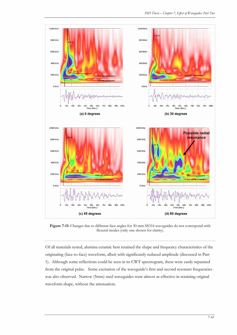
PhD Thesis – Chapter 7, Effect of Waveguides: Part Two
Figure 7-11: Changes due to different face angles for 30-mm SS316 waveguides do not correspond with flexural modes (only one shown for clarity).
Of all materials tested, alumina ceramic best retained the shape and frequency characteristics of the
originating (face-to-face) waveform, albeit with significantly reduced amplitude (discussed in Part
1). Although some reflections could be seen in its CWT spectrogram, these were easily separated
from the original pulse. Some excitation of the waveguide’s first and second resonant frequencies
was also observed. Narrow (5mm) steel waveguides were almost as effective in retaining original
waveform shape, without the attenuation.
7-14
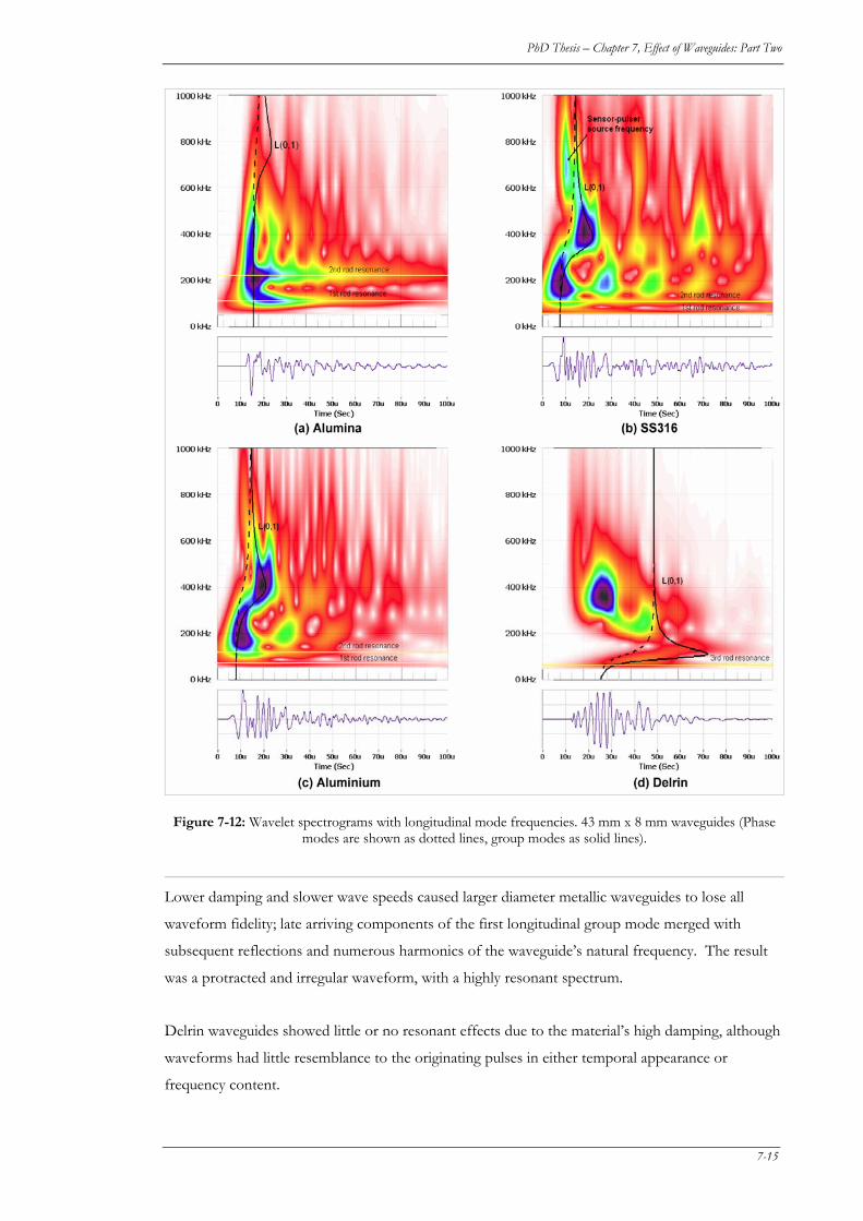
PhD Thesis – Chapter 7, Effect of Waveguides: Part Two
Figure 7-12: Wavelet spectrograms with longitudinal mode frequencies. 43 mm x 8 mm waveguides (Phase modes are shown as dotted lines, group modes as solid lines).
Lower damping and slower wave speeds caused larger diameter metallic waveguides to lose all
waveform fidelity; late arriving components of the first longitudinal group mode merged with
subsequent reflections and numerous harmonics of the waveguide’s natural frequency. The result
was a protracted and irregular waveform, with a highly resonant spectrum.
Delrin waveguides showed little or no resonant effects due to the material’s high damping, although
waveforms had little resemblance to the originating pulses in either temporal appearance or
frequency content.
7-15
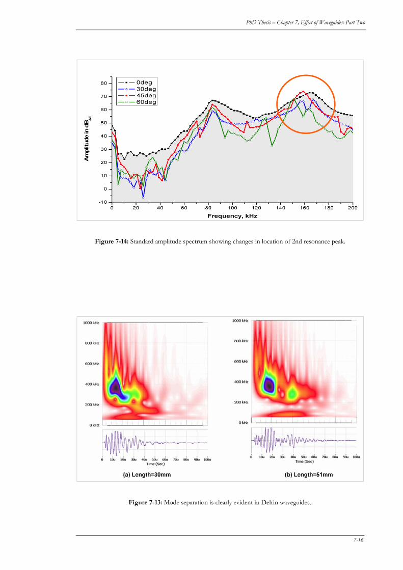
PhD Thesis – Chapter 7, Effect of Waveguides: Part Two
Figure 7-13: Mode separation is clearly evident in Delrin waveguides.
Figure 7-14: Standard amplitude spectrum showing changes in location of 2nd resonance peak.
7-16
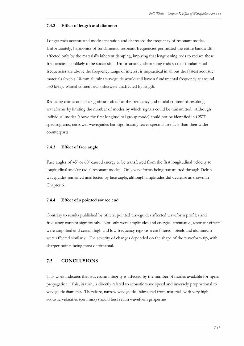
PhD Thesis – Chapter 7, Effect of Waveguides: Part Two
7.4.2 Effect of length and diameter
Longer rods accentuated mode separation and decreased the frequency of resonant modes.
Unfortunately, harmonics of fundamental resonant frequencies permeated the entire bandwidth,
affected only by the material’s inherent damping, implying that lengthening rods to reduce these
frequencies is unlikely to be successful. Unfortunately, shortening rods so that fundamental
frequencies are above the frequency range of interest is impractical in all but the fastest acoustic
materials (even a 10-mm alumina waveguide would still have a fundamental frequency at around
530 kHz). Modal content was otherwise unaffected by length.
Reducing diameter had a significant effect of the frequency and modal content of resulting
waveforms by limiting the number of modes by which signals could be transmitted. Although
individual modes (above the first longitudinal group mode) could not be identified in CWT
spectrograms, narrower waveguides had significantly fewer spectral artefacts than their wider
counterparts.
7.4.3 Effect of face angle
Face angles of 45˚ or 60˚ caused energy to be transferred from the first longitudinal velocity to
longitudinal and/or radial resonant modes. Only waveforms being transmitted through Delrin
waveguides remained unaffected by face angle, although amplitudes did decrease as shown in
Chapter 6.
7.4.4 Effect of a pointed source end
Contrary to results published by others, pointed waveguides affected waveform profiles and
frequency content significantly. Not only were amplitudes and energies attenuated, resonant effects
were amplified and certain high and low frequency regions were filtered. Steels and aluminium
were affected similarly. The severity of changes depended on the shape of the waveform tip, with
sharper points being most detrimental.
7.5 CONCLUSIONS
This work indicates that waveform integrity is affected by the number of modes available for signal
propagation. This, in turn, is directly related to acoustic wave speed and inversely proportional to
waveguide diameter. Therefore, narrow waveguides fabricated from materials with very high
acoustic velocities (ceramics) should best retain waveform properties.
7-17
PhD Thesis – Chapter 7, Effect of Waveguides: Part Two
In commonly used materials such as aluminium, mild steel and stainless steel, longitudinal
resonance artefacts dominate frequency responses in all but very narrow guides. These effects are
magnified by application of a point on the end of a waveguide, or by angling the sensor face, which
also excites radial resonances. Consequently, both should be avoided if trying to maintain
waveform integrity.
Although use of waveguides in AE testing cannot be avoided, their implementation must be
properly considered; dispersion, attenuation, mode conversion and/or waveguide reflections
occurring within the waveguide will affect the signals being detected by the sensor. If possible,
ends should be square and parallel and materials should be selected depending on the transmission
characteristics required for a particular monitoring task. If possible, specific designs should be
tested prior to installation so that transmission characteristics can be verified.
7-18

8. FFLLOOWW MMOONNIITTOORRIINNGG OOFF
AA DDOOUUBBLLEE--SSUUCCTTIIOONN PPUUMMPP
Sikorska, J. and Hodkiewicz, M.,
Proceedings of the Comadem 2005,
pp. 192-202.
88
The aims of this chapter are to:
(a) Verify whether changes in hydraulic conditions in a double suction pump can be
monitored using acoustic emission; and
(b) Determine if acoustic emission can detect these conditions more accurately that dynamic
pressure or vibration monitoring.
Publication Abstract
Measurements from acoustic emission, vibration and dynamic pressure transducers are presented
for a range of flows and two pump speeds on a double-suction centrifugal pump. These show the
AE signals are more sensitive to change in flow condition away from the pump’s best-efficiency
point than either vibration or dynamic pressure measurement. Results indicate that AE monitoring
may therefore be appropriate for determining the location of best efficiency and for detecting the
onset of undesirable hydraulic conditions such as recirculation and cavitation.
8.1 INTRODUCTION
A centrifugal pump moves fluid from one point to another by converting mechanical energy into
hydraulic energy, which is referred to as head and is measured in meters. The efficiency of the
mechanical-hydraulic energy conversion varies with flow (Figure 8-1a). Input energy is most
efficiently converted into increased head at a single flowrate called the Best Efficiency Point (BEP).
8-1
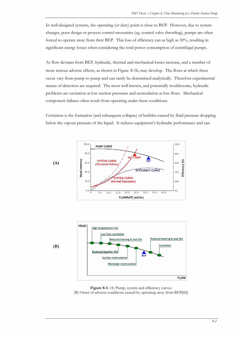
PhD Thesis – Chapter 8, Flow Monitoring of a Double Suction Pump
In well-designed systems, the operating (or duty) point is close to BEP. However, due to system
changes, poor design or process control necessities (eg. control valve throttling), pumps are often
forced to operate away from their BEP. This loss of efficiency can as high as 30%, resulting in
significant energy losses when considering the total power consumption of centrifugal pumps.
As flow deviates from BEP, hydraulic, thermal and mechanical losses increase, and a number of
more serious adverse effects, as shown in Figure 8-1b, may develop. The flows at which these
occur vary from pump to pump and can rarely be determined analytically. Therefore experimental
means of detection are required. The most well known, and potentially troublesome, hydraulic
problems are cavitation at low suction pressures and recirculation at low flows. Mechanical
component failures often result from operating under these conditions.
Cavitation is the formation (and subsequent collapse) of bubbles caused by fluid pressure dropping
below the vapour pressure of the liquid. It reduces equipment’s hydraulic performance and can
(A)
(B)
Figure 8-1: (A) Pump, system and efficiency curves. (B) Onset of adverse conditions caused by operating away from BEP[60].
8-2
PhD Thesis – Chapter 8, Flow Monitoring of a Double Suction Pump
result in significant noise, vibration, pressure pulsations and erosion to metal surfaces. To avoid
cavitation damage, manufacturers recommend that a pump operates with suction pressure that
exceeds its minimum net positive suction head required (NPSHR), which is an experimentally
determined value derived from the pressure at which total discharge head drops by 3% (flow kept
constant). From the perspective of the research work described herein, it is important to recognise
that cavitation starts occurring (called incipient cavitation) at suction pressures significantly above
NPSH; most pumps routinely operate satisfactorily with some level of incipient cavitation.
Cavitation effects increase with flow due primarily to additional friction losses incurred in suction
piping reducing the available suction pressure at the pump’s inlet.
At low flows, fluid reverses back from the impeller into the inlet pipe, travelling along its outside
diameter creating a rotating field. When this reversal occurs at the inlet eye it is know as suction
recirculation, whilst if it occurs at the discharge tips of the impeller vanes it is called discharge
recirculation. The amount of flow reversal increases as flow is reduced. In most pumps, the
capacities at which suction and discharge recirculation commence differ, although generally (but not
always) suction recirculation will commence at a higher flow than discharge recirculation [37].
Damage associated with either form of recirculation is more likely in high energy pumps [20].
8.2 DETECTION OF ADVERSE HYDRAULIC CONDITIONS
Determining where a pump is operating on its curve at any instant is typically done by measuring
flow or discharge pressure and then comparing readings to the pump’s head-flow curve. A typical
curve is shown in Figure 8-1. In practice there are a number of difficulties with this approach: (i)
the pump curve is only valid for a new pump, (ii) the shape and location of the curve may change
due to wear, and (iii) only a small percentage of pumps have associated flow measuring devices.
A number of methods have therefore been trialled over the past fifty years to detect damaging
hydraulic conditions in centrifugal machines. These include visual observation, dynamic pressure,
vibration, sound (both internally and externally) and more recently acoustic emission. Only the
latter three methods do not require special pumps or intrusive instrumentation. The key findings of
this body of previous work are now summarised.
8.2.1 Stable Cavitation (low NPSHA)
Stable cavitation is generally observed as high frequency pulses in vibration, acoustic and pressure
signals, of random duration and amplitude, superimposed over a level of broadband noise from the
pump [42, 66]. As the degree of cavitation increases, the amplitude of casing vibrations, noise and
dynamic pressure fluctuations rise significantly. The magnitude of pressure pulsations caused by
8-3
PhD Thesis – Chapter 8, Flow Monitoring of a Double Suction Pump
stable cavitation are dependant on the pump-impeller geometry [19, 27]. Furthermore, overall
noise and vibration levels are a function of operating conditions (NPSHA, flow and speed) and
pump design [63, 101, 111]. Under stable cavitation, broadband vibrations can also modulate
specific frequencies (running speed, vane pass frequency, 0.5 x vane pass frequency). Increases at
these specific frequencies have been measured with vibration [7, 58] and acoustic sensors [28, 111].
The generation of acoustic emissions during bubble formation and collapse was first identified by
Derakshan in 1977, who also determined that cavitation intensity in a hydro-turbine was
proportional to the RMS (root mean square) of the acoustic emission signal [29]. Since then others
have reported that cavitation in machinery can be detected by “high amplitude excursions in the
RMS” [34]. Crest factors (ratio of the signal peak to its RMS) have been suggested as more reliable
indicators of incipient cavitation than RMS because during cavitation, acoustic emission bursts
typically have very high peak values with respect to the background noise level [66, 80, 81], but no
work in this has been published.
Frequency analysis of AE spectra has also been used to identify cavitation. In work by Neill et al,
the AE spectrum was very similar in shape to that under rated duty, but up to 40dBAE higher in
amplitude (depending on the degree of cavitation and sensor location). A sudden decrease in the
high frequency energy (0.5-1MHz) was also observed as cavitation developed [80, 81].
8.2.2 Recirculation
Collective research suggests that discharge recirculation can appear very similar to cavitation:
broadband pressure pulsations increase, as do levels at specific frequencies such as the blade-pass
frequency [41]. Suction recirculation on the other hand tends to increase mainly the low frequency
pressure pulsations (<125Hz) and dampens high frequencies [41]. The amplitude of pressure
pulsations increases with the intensity of recirculation. Pressure pulsations at 10-75Hz were also
observed by others under low flow conditions, who were unable to determine if these were due to
suction or discharge recirculation [47]. Unfortunately, dynamic pressure measurements are very
sensitive to sensor location, reducing with distance from the pump.
Under low flow conditions, low frequency axial vibrations have also been measured on the non-
drive end bearing housing of single stage, double suction horizontal pumps [49, 82].
Limited research on the use of AE for detecting low flow conditions has been reported. These
indicate that raw AE signals during recirculation tend to be mixed mode (bursts superimposed over
a background level of broadband AE), with little change in the background levels from non-
recirculating conditions, but with much larger discrete events [80, 81]. As for cavitation, Neill
8-4
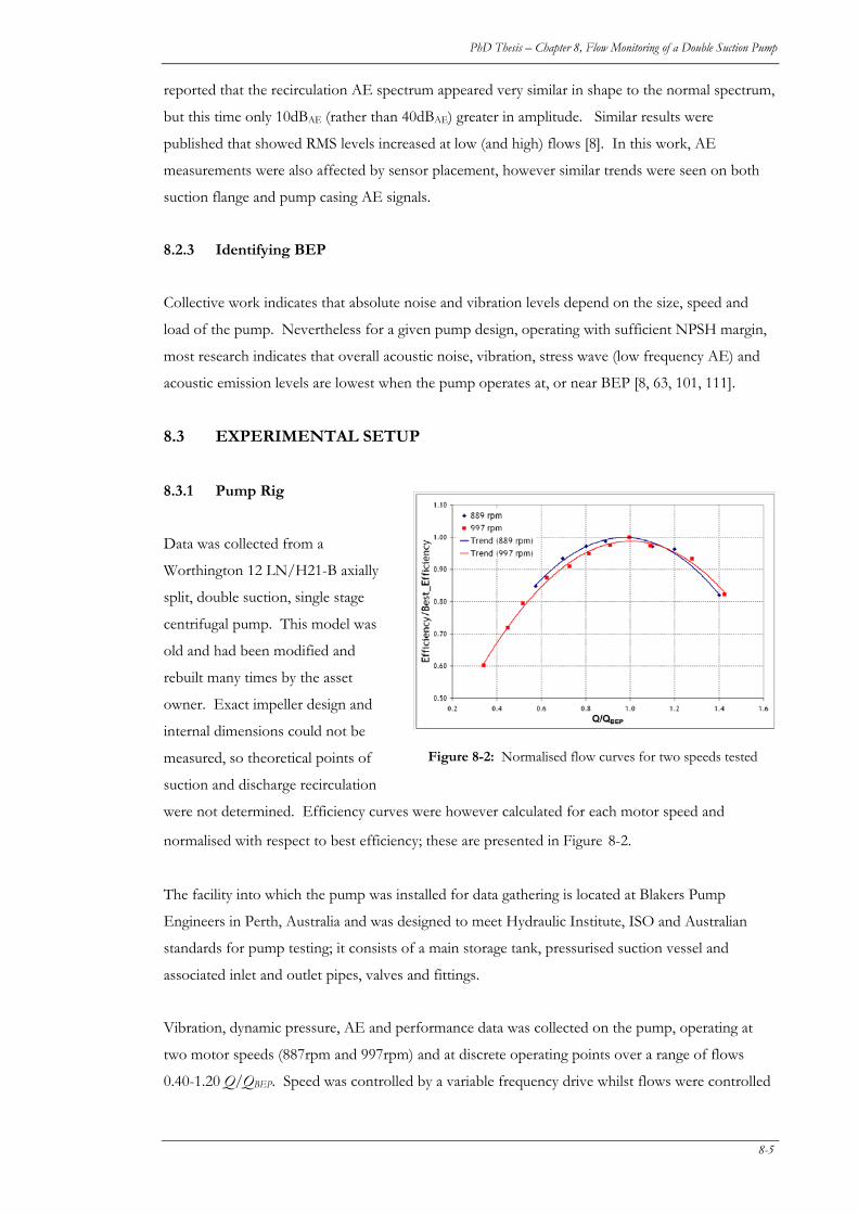
PhD Thesis – Chapter 8, Flow Monitoring of a Double Suction Pump
reported that the recirculation AE spectrum appeared very similar in shape to the normal spectrum,
but this time only 10dBAE (rather than 40dBAE) greater in amplitude. Similar results were
published that showed RMS levels increased at low (and high) flows [8]. In this work, AE
measurements were also affected by sensor placement, however similar trends were seen on both
suction flange and pump casing AE signals.
8.2.3 Identifying BEP
Collective work indicates that absolute noise and vibration levels depend on the size, speed and
load of the pump. Nevertheless for a given pump design, operating with sufficient NPSH margin,
most research indicates that overall acoustic noise, vibration, stress wave (low frequency AE) and
acoustic emission levels are lowest when the pump operates at, or near BEP [8, 63, 101, 111].
8.3 EXPERIMENTAL SETUP
8.3.1 Pump Rig
Data was collected from a
Worthington 12 LN/H21-B axially
split, double suction, single stage
centrifugal pump. This model was
old and had been modified and
rebuilt many times by the asset
owner. Exact impeller design and
internal dimensions could not be
measured, so theoretical points of
suction and discharge recirculation
were not determined. Efficiency curves were however calculated for each motor speed and
normalised with respect to best efficiency; these are presented in Figure 8-2
Figure 8-2: Normalised flow curves for two speeds tested
.
The facility into which the pump was installed for data gathering is located at Blakers Pump
Engineers in Perth, Australia and was designed to meet Hydraulic Institute, ISO and Australian
standards for pump testing; it consists of a main storage tank, pressurised suction vessel and
associated inlet and outlet pipes, valves and fittings.
Vibration, dynamic pressure, AE and performance data was collected on the pump, operating at
two motor speeds (887rpm and 997rpm) and at discrete operating points over a range of flows
0.40-1.20 Q/QBEP. Speed was controlled by a variable frequency drive whilst flows were controlled
8-5
PhD Thesis – Chapter 8, Flow Monitoring of a Double Suction Pump
by manually adjusting the position of a valve downstream of the pump. The results of these tests
are reported in the following section. Additional tests involving reducing the suction pressure to
the pump were also conducted and associated results will be reported in a separate publication.
8.3.2 Vibration and Pressure (MH)
At each operating point 150 seconds of vibration and dynamic pressure sensor data was digitally
recorded using a Sony Tape recorder from B&K 4396 Deltatron accelerometers and PCB 112A22
dynamic pressure transducers. Performance data providing flow, pressure, motor power and pump
efficiency was also recorded. One accelerometer was placed on the non-drive end pump bearing
housing in line with the pump shaft axis and another was mounted on the discharge flange of the
pump. Dynamic pressure transducers were placed in ports located directly on the suction and
discharge nozzles of the pump.
Signals from the digital tape recorder were subsequently down-sampled at 2048 Hz using a National
Instrument PCI-4552 board providing four channels of simultaneous 16-bit data. Signal processing
thereafter used purpose-built LabVIEW and Matlab programs as described in [48, 49] to determine
statistical parameters of the signals and perform joint time frequency analysis.
8.3.3 AE Measurement
AE signals were measured using three Physical Acoustics wideband sensors (WD/WDI/WDIS),
each with 46dB total analog gain. These were placed on the suction and discharge flanges and
pump casing, held in place by magnetic mounts. Silicon grease was used as the couplant.
Signals were collected using two Physical Acoustics PCI2 boards installed into a 2.8GHz clone PC,
running AEWin for PCI2. In addition to all hit information, time dependant AE parameters were
collected every 10 seconds and waveform files (2048576 samples) every 30 seconds. A floating
trigger was set at 20dB (above the ASL). All channels were passed through analog bandpass filters,
set at 100-1000kHz, and signals were then digitised at 2MHz. Data was extracted and analysed
using a SQL server based data management and analysis system as detailed in [108].
Swansong II [35] and inverse Swansong II filters were applied to hit data sets to separate impulsive
burst data from continuous AE hits. Unfiltered hit data was also analysed to determine the
effectiveness of these filters.
AE waveform files were post-processed to determine: (a) traditional statistics (eg. RMS, Peak,
Kurtosis, Crest Factor), (b) 1/3rd octave band powers and (c) discrete wavelet level energies. In the
8-6
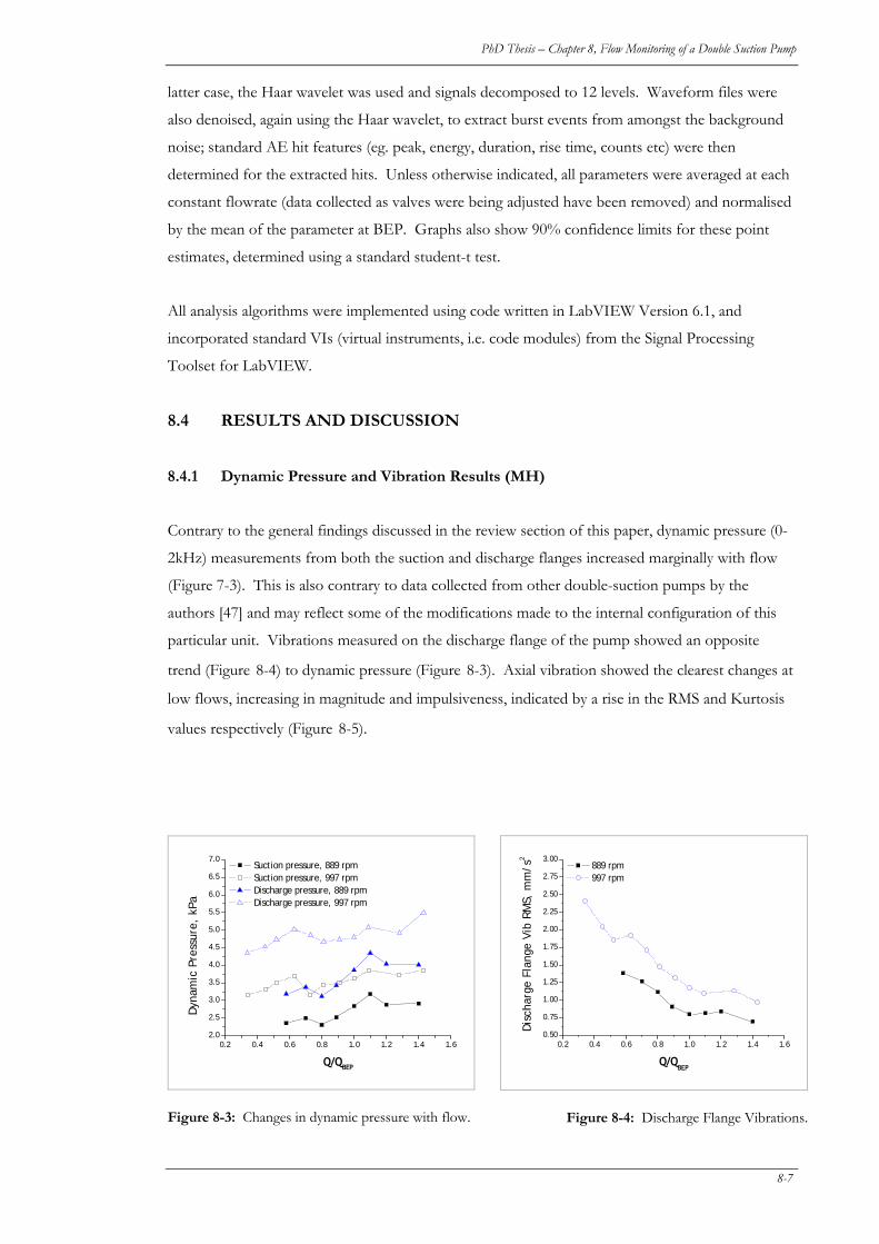
PhD Thesis – Chapter 8, Flow Monitoring of a Double Suction Pump
latter case, the Haar wavelet was used and signals decomposed to 12 levels. Waveform files were
also denoised, again using the Haar wavelet, to extract burst events from amongst the background
noise; standard AE hit features (eg. peak, energy, duration, rise time, counts etc) were then
determined for the extracted hits. Unless otherwise indicated, all parameters were averaged at each
constant flowrate (data collected as valves were being adjusted have been removed) and normalised
by the mean of the parameter at BEP. Graphs also show 90% confidence limits for these point
estimates, determined using a standard student-t test.
All analysis algorithms were implemented using code written in LabVIEW Version 6.1, and
incorporated standard VIs (virtual instruments, i.e. code modules) from the Signal Processing
Toolset for LabVIEW.
8.4 RESULTS AND DISCUSSION
8.4.1 Dynamic Pressure and Vibration Results (MH)
Contrary to the general findings discussed in the review section of this paper, dynamic pressure (0-
2kHz) measurements from both the suction and discharge flanges increased marginally with flow
(Figure 7-3). This is also contrary to data collected from other double-suction pumps by the
authors [47] and may reflect some of the modifications made to the internal configuration of this
particular unit. Vibrations measured on the discharge flange of the pump showed an opposite
trend (Figure 8-4) to dynamic pressure (Figure 8-3). Axial vibration showed the clearest changes at
low flows, increasing in magnitude and impulsiveness, indicated by a rise in the RMS and Kurtosis
values respectively (Figure 8-5).
0.2 0.4 0.6 0.8 1.0 1.2 1.4 1.60.50
0.75
1.00
1.25
1.50
1.75
2.00
2.25
2.50
2.75
3.00 889 rpm 997 rpm
Dis
char
ge F
lang
e Vi
b RM
S, m
m/s
2
Q/QBEP
Figure 8-4: Discharge Flange Vibrations.
0.2 0.4 0.6 0.8 1.0 1.2 1.4 1.62.0
2.5
3.0
3.5
4.0
4.5
5.0
5.5
6.0
6.5
7.0
Dyn
amic
Pre
ssur
e, k
Pa
Q/QBEP
Suction pressure, 889 rpm Suction pressure, 997 rpm Discharge pressure, 889 rpm Discharge pressure, 997 rpm
Figure 8-3: Changes in dynamic pressure with flow.
8-7
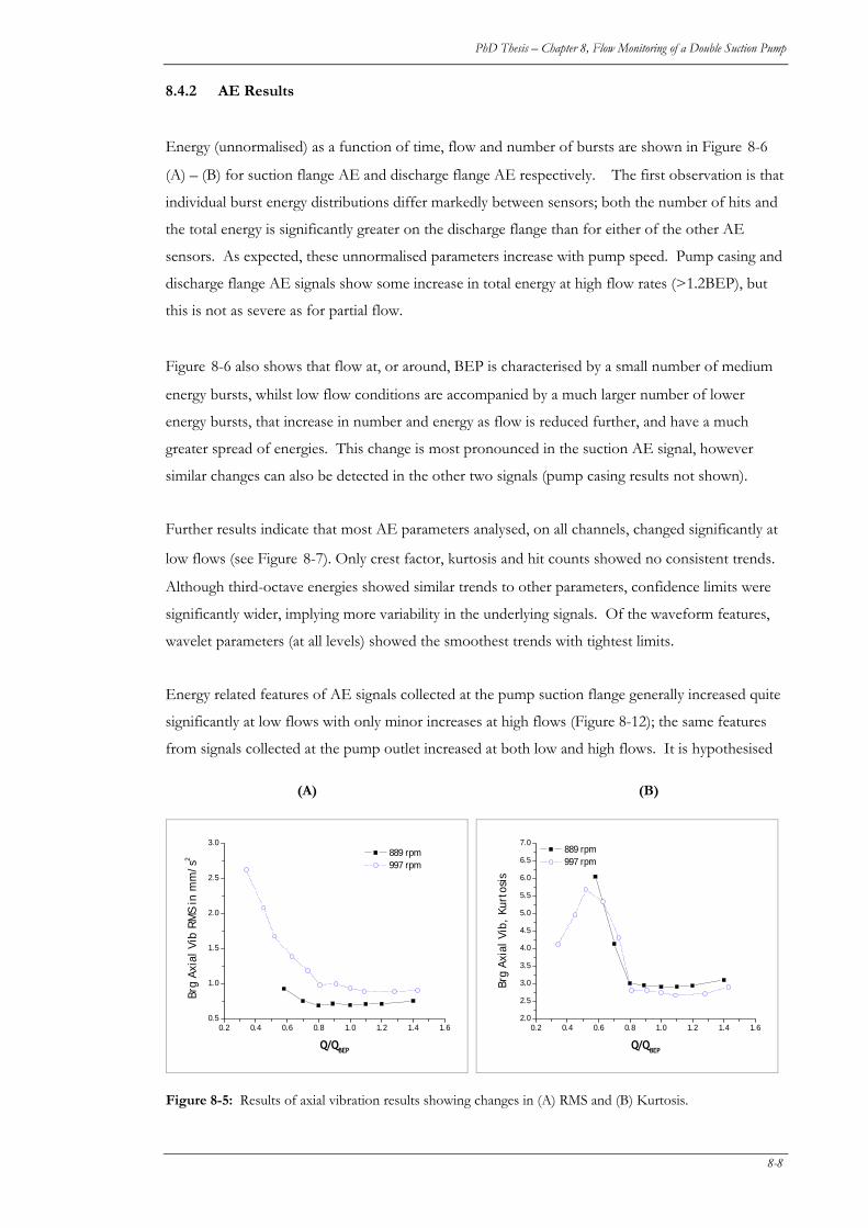
PhD Thesis – Chapter 8, Flow Monitoring of a Double Suction Pump
8.4.2 AE Results
Energy (unnormalised) as a function of time, flow and number of bursts are shown in Figure 8-6
(A) – (B) for suction flange AE and discharge flange AE respectively. The first observation is that
individual burst energy distributions differ markedly between sensors; both the number of hits and
the total energy is significantly greater on the discharge flange than for either of the other AE
sensors. As expected, these unnormalised parameters increase with pump speed. Pump casing and
discharge flange AE signals show some increase in total energy at high flow rates (>1.2BEP), but
this is not as severe as for partial flow.
Figure 8-6 also shows that flow at, or around, BEP is characterised by a small number of medium
energy bursts, whilst low flow conditions are accompanied by a much larger number of lower
energy bursts, that increase in number and energy as flow is reduced further, and have a much
greater spread of energies. This change is most pronounced in the suction AE signal, however
similar changes can also be detected in the other two signals (pump casing results not shown).
Further results indicate that most AE parameters analysed, on all channels, changed significantly at
low flows (see Figure 8-7). Only crest factor, kurtosis and hit counts showed no consistent trends.
Although third-octave energies showed similar trends to other parameters, confidence limits were
significantly wider, implying more variability in the underlying signals. Of the waveform features,
wavelet parameters (at all levels) showed the smoothest trends with tightest limits.
Energy related features of AE signals collected at the pump suction flange generally increased quite
significantly at low flows with only minor increases at high flows (Figure 8-12); the same features
from signals collected at the pump outlet increased at both low and high flows. It is hypothesised
(A) (B)
0.2 0.4 0.6 0.8 1.0 1.2 1.4 1.60.5
1.0
1.5
2.0
2.5
3.0
Brg
Axia
l Vi
b RM
S in
mm
/s2
Q/QBEP
889 rpm 997 rpm
0.2 0.4 0.6 0.8 1.0 1.2 1.4 1.62.0
2.5
3.0
3.5
4.0
4.5
5.0
5.5
6.0
6.5
7.0 889 rpm 997 rpm
Brg
Axia
l Vib
, Ku
rtos
is
Q/QBEP
Figure 8-5: Results of axial vibration results showing changes in (A) RMS and (B) Kurtosis.
8-8
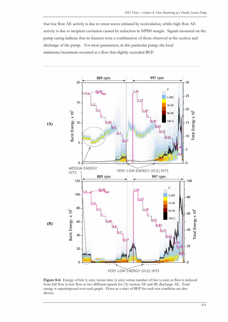
PhD Thesis – Chapter 8, Flow Monitoring of a Double Suction Pump
that low flow AE activity is due to stress waves initiated by recirculation, whilst high flow AE
activity is due to incipient cavitation caused by reduction in NPSH margin. Signals mounted on the
pump casing indicate that its features were a combination of those observed at the suction and
discharge of the pump. For most parameters, in this particular pump, the local
minimum/maximum occurred at a flow that slightly exceeded BEP.
Figure 8-6: Energy of hits (y axis) versus time (x axis) versus number of hits (z axis) as flow is reduced from full flow to low flow at two different speeds for (A) suction AE and (B) discharge AE. Total energy is superimposed over each graph. Flows as a ratio of BEP for each test condition are also shown.
(A)
(B)
8-9
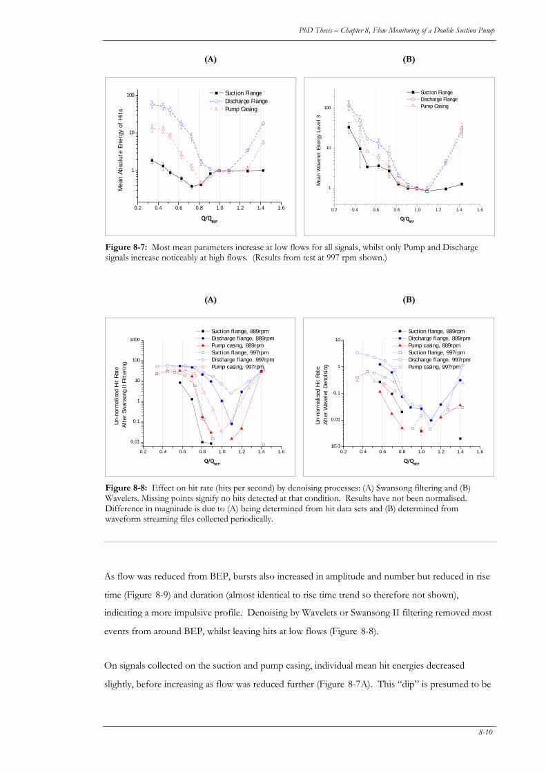
PhD Thesis – Chapter 8, Flow Monitoring of a Double Suction Pump
As flow was reduced from BEP, bursts also increased in amplitude and number but reduced in rise
time (Figure 8-9) and duration (almost identical to rise time trend so therefore not shown),
indicating a more impulsive profile. Denoising by Wavelets or Swansong II filtering removed most
events from around BEP, whilst leaving hits at low flows (Figure 8-8).
On signals collected on the suction and pump casing, individual mean hit energies decreased
slightly, before increasing as flow was reduced further (Figure 8-7A). This “dip” is presumed to be
(A) (B)
0.2 0.4 0.6 0.8 1.0 1.2 1.4 1.6
1
10
100
Q/QBEP
Suction Flange Discharge Flange Pump Casing
Mea
n Ab
solu
te E
nerg
y of
Hit
s
0.2 0.4 0.6 0.8 1.0 1.2 1.4 1.6
1
10
100
Q/QBEP
Suction Flange Discharge Flange Pump Casing
Mea
n W
avel
et E
nerg
y Le
vel 3
Figure 8-7: Most mean parameters increase at low flows for all signals, whilst only Pump and Discharge signals increase noticeably at high flows. (Results from test at 997 rpm shown.)
(A) (B)
0.2 0.4 0.6 0.8 1.0 1.2 1.4 1.6
0.01
0.1
1
10
100
1000
Un-
norm
alis
ed H
it R
ate
Afte
r Sw
anso
ng II
Filt
erin
g
Q/QBEP
Suction flange, 889rpm Discharge flange, 889rpm Pump casing, 889rpm Suction flange, 997rpm Discharge flange, 997rpm Pump casing, 997rpm
0.2 0.4 0.6 0.8 1.0 1.2 1.4 1.61E-3
0.01
0.1
1
10
Un-
norm
alis
ed H
it R
ate
Afte
r W
avel
et D
enoi
sing
Q/QBEP
Suction flange, 889rpm Discharge flange, 889rpm Pump casing, 889rpm Suction flange, 997rpm Discharge flange, 997rpm Pump casing, 997rpm
Figure 8-8: Effect on hit rate (hits per second) by denoising processes: (A) Swansong filtering and (B) Wavelets. Missing points signify no hits detected at that condition. Results have not been normalised. Difference in magnitude is due to (A) being determined from hit data sets and (B) determined from waveform streaming files collected periodically.
8-10
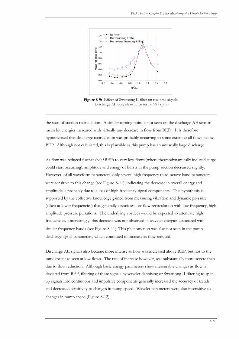
PhD Thesis – Chapter 8, Flow Monitoring of a Double Suction Pump
the start of suction recirculation. A similar turning point is not seen on the discharge AE sensor:
mean hit energies increased with virtually any decrease in flow from BEP. It is therefore
hypothesised that discharge recirculation was probably occurring to some extent at all flows below
BEP. Although not calculated, this is plausible as this pump has an unusually large discharge.
As flow was reduced further (<0.5BEP) to very low flows (where thermodynamically induced surge
could start occurring), amplitude and energy of bursts in the pump suction decreased slightly.
However, of all waveform parameters, only several high frequency third-octave band parameters
were sensitive to this change (see Figure 8-11), indicating the decrease in overall energy and
amplitude is probably due to a loss of high frequency signal components. This hypothesis is
supported by the collective knowledge gained from measuring vibration and dynamic pressure
(albeit at lower frequencies) that generally associates low flow recirculation with low frequency, high
amplitude pressure pulsations. The underlying vortices would be expected to attenuate high
frequencies. Interestingly, this decrease was not observed in wavelet energies associated with
similar frequency bands (see Figure 8-11). This phenomenon was also not seen in the pump
discharge signal parameters, which continued to increase as flow reduced.
Discharge AE signals also became more intense as flow was increased above BEP, but not to the
same extent as seen at low flows. The rate of increase however, was substantially more severe than
due to flow reduction. Although basic energy parameters show measurable changes as flow is
deviated from BEP, filtering of these signals by wavelet denoising or Swansong II filtering to split
up signals into continuous and impulsive components generally increased the accuracy of trends
and decreased sensitivity to changes in pump speed. Wavelet parameters were also insensitive to
changes in pump speed (Figure 8-12).
0.2 0.4 0.6 0.8 1.0 1.2 1.4 1.60.0
0.2
0.4
0.6
0.8
1.0
1.2
1.4
1.6 No Filter Post Swansong II filter Post Inverse Swansong II filter
Mea
n H
it R
ise
Tim
e
Q/QBEP
Figure 8-9: Effect of Swansong II filter on rise time signals.
(Discharge AE only shown, for test at 997 rpm.)
8-11
PhD Thesis – Chapter 8, Flow Monitoring of a Double Suction Pump
8.5 CONCLUSIONS AND RECOMMENDATIONS
This work indicates that acoustic emission can be a powerful and sensitive tool for detecting off
duty conditions in double suction pumps, presumably because the acoustic emission events relate
directly to pressure pulsations occurring within the fluid. Expected changes associated with off-
duty conditions can be clearly observed in hit-time intensity plots, which as shown by previous
research, are affected significantly by sensor position. Although basic energy parameters show
measurable changes as flow is deviated from BEP, further post processing of these signals
improves the accuracy of trends and decreases sensitivity to changes in pump speed. Results
indicate that on this particular double suction pump, collecting acoustic emission signals from
suction and discharge flanges can clearly identify the changes occurring within the pump that may
be associated with the onset of suction recirculation, discharge recirculation and incipient
cavitation. This research also shows that acoustic emission can be a more useful tool for analysing
hydraulic activity than traditional techniques such as dynamic pressure and/or vibration
monitoring. However, further testing is required on a variety of centrifugal pumps to determine if
they all show similar trends.
8-12
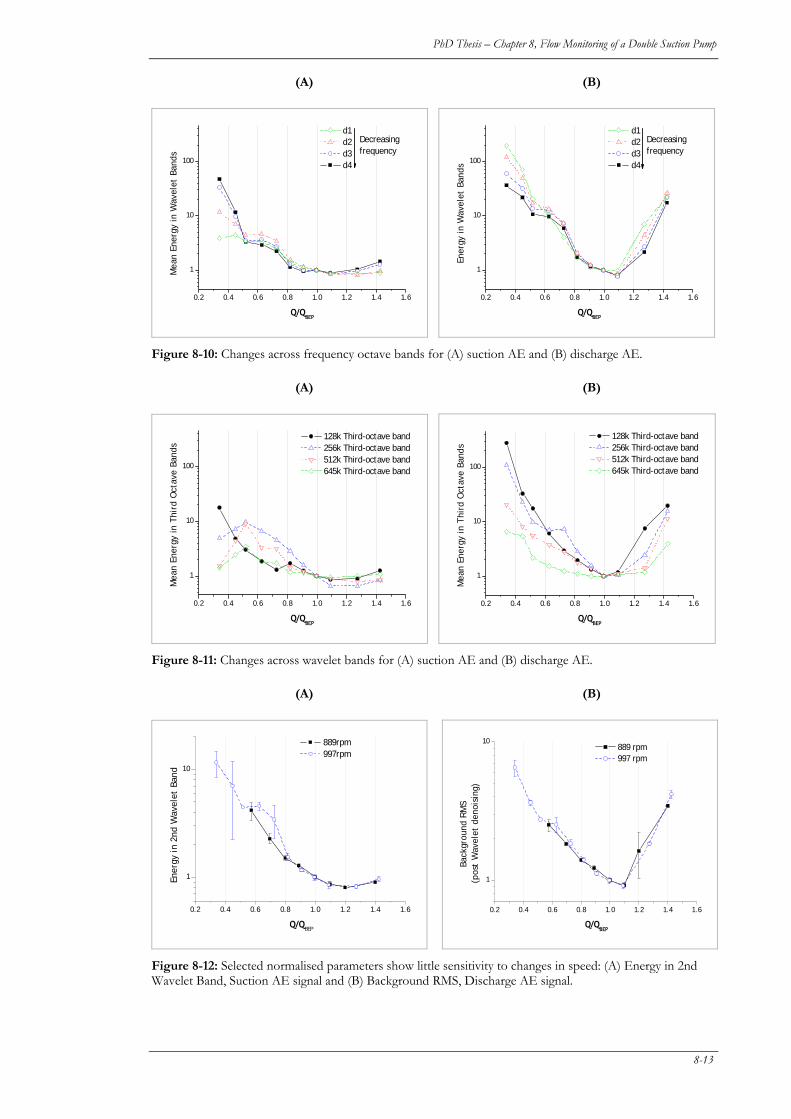
PhD Thesis – Chapter 8, Flow Monitoring of a Double Suction Pump
(A) (B)
0.2 0.4 0.6 0.8 1.0 1.2 1.4 1.6
1
10
100
Mea
n En
ergy
in W
avel
et B
ands
Q/QBEP
d1 d2 d3 d4
Decreasing frequency
0.2 0.4 0.6 0.8 1.0 1.2 1.4 1.6
1
10
100
Ener
gy in
Wav
elet
Ban
ds
Q/QBEP
d1 d2 d3 d4
Decreasing frequency
Figure 8-10: Changes across frequency octave bands for (A) suction AE and (B) discharge AE.
(A) (B)
0.2 0.4 0.6 0.8 1.0 1.2 1.4 1.6
1
10
100
Mea
n En
ergy
in T
hird
Oct
ave
Band
s
Q/QBEP
128k Third-octave band 256k Third-octave band 512k Third-octave band 645k Third-octave band
0.2 0.4 0.6 0.8 1.0 1.2 1.4 1.6
1
10
100M
ean
Ener
gy in
Thi
rd O
ctav
e Ba
nds
Q/QBEP
128k Third-octave band 256k Third-octave band 512k Third-octave band 645k Third-octave band
Figure 8-11: Changes across wavelet bands for (A) suction AE and (B) discharge AE.
(A) (B)
0.2 0.4 0.6 0.8 1.0 1.2 1.4 1.6
1
10
889rpm 997rpm
Q/QBEP
Ener
gy in
2nd
Wav
elet
Ban
d
0.2 0.4 0.6 0.8 1.0 1.2 1.4 1.6
1
10 889 rpm 997 rpm
Q/QBEP
Back
grou
nd R
MS
(pos
t W
avel
et d
enoi
sing
)
Figure 8-12: Selected normalised parameters show little sensitivity to changes in speed: (A) Energy in 2nd Wavelet Band, Suction AE signal and (B) Background RMS, Discharge AE signal.
8-13
9. FFLLOOWW MMOONNIITTOORRIINNGG OOFF
EENNDD--SSUUCCTTIIOONN PPUUMMPPSS
The aims of this chapter are to:
(a) Present the results of flow tests conducted on a number of single stage centrifugal pumps;
(b) Discuss the sensitivity of AE results to the testing process.
Abstract
99
A review of literature discussing the suitability of acoustic emission monitoring for detecting and
identifying off-duty and potentially damaging hydraulic conditions in centrifugal pumps was
presented in [107] and Chapter 8. The experimental and data processing methods were also
outlined therein. This chapter presents the results of flow tests conducted on a variety of smaller,
new, end suction pumps so that potential similarities and differences can be identified. All data was
collected on pumps being tested at Blakers Pumps’ test facility and processed using the techniques
described previously in this thesis.
9.1 INTRODUCTION
Part of the pre-commissioning process for many ANSI and API pumps is a pre-acceptance test to
verify the head-flow and efficiency-flow characteristics of the specific unit. These performance
tests are conducted in accordance with relevant pump standards [1, 116] on specially designed test
rigs at the supplier’s or manufacturer’s premises and may be witnessed by the customer. Testing
involves installing a new pump on the test rig and running it at various flows. Pressures, flows,
motor current, supply voltage, motor speed, VFD frequency and fluid temperatures are measured at
9-1
PhD Thesis – Chapter 9, Flow Monitoring of End-suction Pumps
each flow and the resulting head-flow and efficiency-flow curves are calculated. These are then
checked against allowable acceptance criteria. This is the easiest and most convenient time to
collect condition-monitoring data for the purposes of benchmarking new pumps, so it was
considered useful to determine if AE monitoring during this process was practical.
As will be discussed in this chapter, it was very difficult to obtain good quality AE data during
acceptance testing for a number of reasons. Typically such results would be removed from the data
set and not presented in published results. However these problems affect the applicability of AE
as a practical monitoring technique and suggest a further challenge, in addition to those listed in the
introduction to this thesis that must be overcome before valid, repeatable and reproducible results
are obtained from every pump test.
9.2 EXPERIMENTAL SETUP
AE data was collected from six new Gould’s single-stage end-suction centrifugal ANSI 3196 or API
670 process pumps at Blakers’ pump test facility. These are designated as Pumps 2, 4, 5, 6, 7 and 8.
Details of each pump are given in Appendix E.
Tests were conducted in two groups: Group 1 consisted of Pumps 2, 4 and 5 whilst Group 2
contained Pumps 6 to 8. Group 1 tests were performed at one motor speed, whilst Group 2 tests
were undertaken at two different motor speeds.
The author preferred not to acquire data during customer witnessed acceptance testing as this was
generally conducted very quickly and very little AE data could be collected from each flow
condition. If time permitted, AE data was collected immediately proceeding, or after the official
tests whilst the pump was installed on the test rig. Unfortunately, it was not uncommon for Blakers
to need to test multiple pumps in one day, so this additional time was often unavailable, thereby
necessitating the collection of data during witness-tests.
9.2.1 DAQ Hardware and Software
Group 1 data was collected using purpose- built AE electronics, a generic data acquisition board by
National Instruments (PCI-6110) and data acquisition software developed in LabVIEW (described
in Appendix B), whilst Group 2 data was collected using commercial off the shelf (COTS)
hardware and software by Physical Acoustics (as described in [107] and Chapter 8). The primary
differences between the acquisition platforms were (a) noise immunity, (b) maximum hit data
capture rates and (c) pre-triggering capability; in all cases the COTS system was superior.
9-2
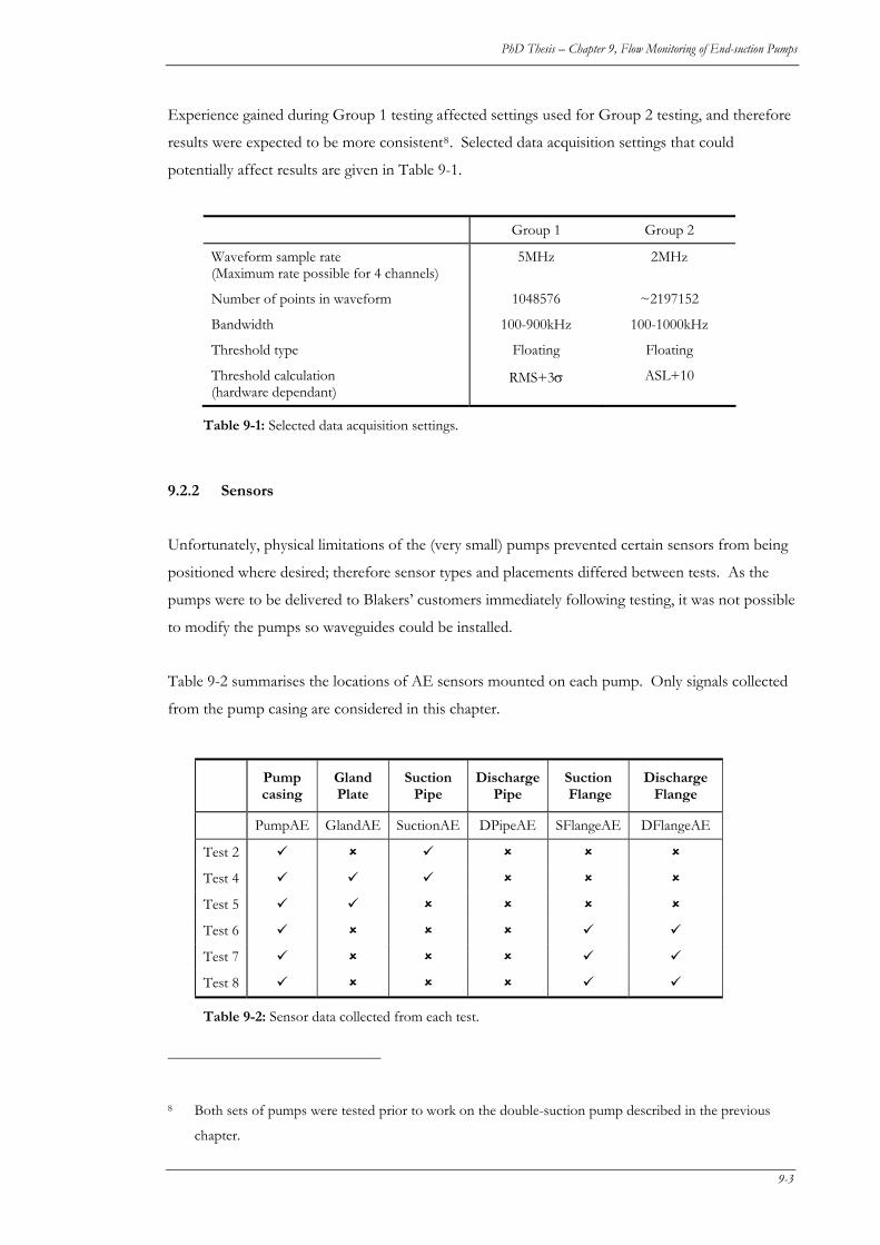
PhD Thesis – Chapter 9, Flow Monitoring of End-suction Pumps
Experience gained during Group 1 testing affected settings used for Group 2 testing, and therefore
results were expected to be more consistent8. Selected data acquisition settings that could
potentially affect results are given in Table 9-1.
Group 1 Group 2
Waveform sample rate (Maximum rate possible for 4 channels)
5MHz 2MHz
Number of points in waveform 1048576 ~2197152
Bandwidth 100-900kHz 100-1000kHz
Threshold type Floating Floating
Threshold calculation (hardware dependant)
ASL+10 RMS+3σ
Table 9-1: Selected data acquisition settings.
9.2.2 Sensors
Unfortunately, physical limitations of the (very small) pumps prevented certain sensors from being
positioned where desired; therefore sensor types and placements differed between tests. As the
pumps were to be delivered to Blakers’ customers immediately following testing, it was not possible
to modify the pumps so waveguides could be installed.
Table 9-2 summarises the locations of AE sensors mounted on each pump. Only signals collected
from the pump casing are considered in this chapter.
Pump casing
Gland Plate
Suction Pipe
DischargePipe
Suction Flange
Discharge Flange
PumpAE GlandAE SuctionAE DPipeAE SFlangeAE DFlangeAE
Test 2
Test 4
Test 5
Test 6
Test 7
Test 8
Table 9-2: Sensor data collected from each test.
8 Both sets of pumps were tested prior to work on the double-suction pump described in the previous
chapter.
9-3
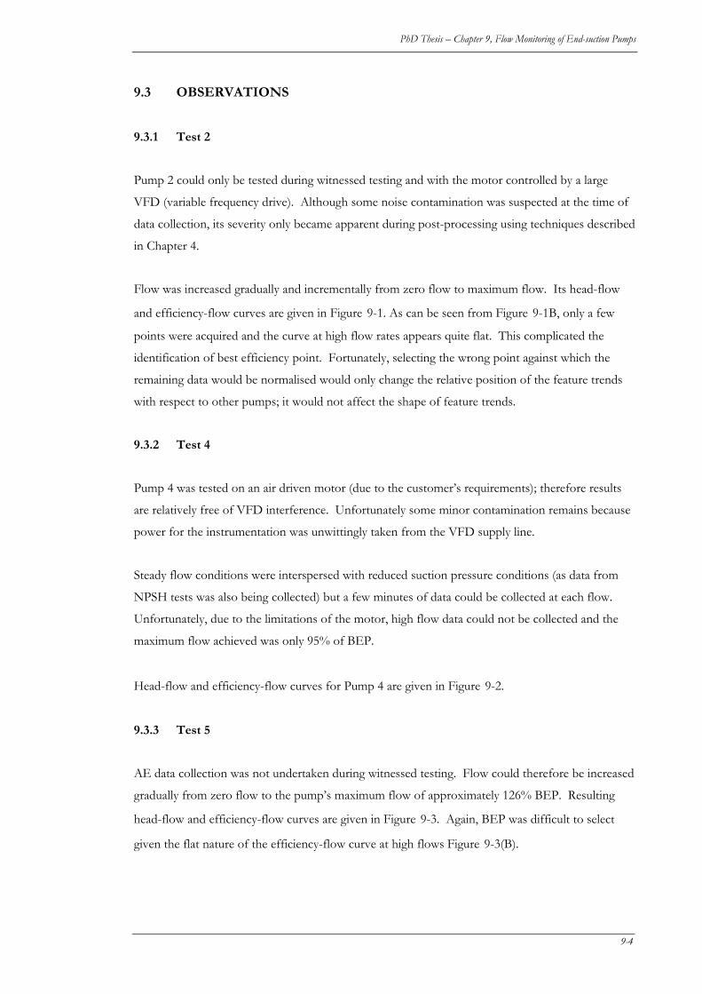
PhD Thesis – Chapter 9, Flow Monitoring of End-suction Pumps
9.3 OBSERVATIONS
9.3.1 Test 2
Pump 2 could only be tested during witnessed testing and with the motor controlled by a large
VFD (variable frequency drive). Although some noise contamination was suspected at the time of
data collection, its severity only became apparent during post-processing using techniques described
in Chapter 4.
Flow was increased gradually and incrementally from zero flow to maximum flow. Its head-flow
and efficiency-flow curves are given in Figure 9-1. As can be seen from Figure 9-1B, only a few
points were acquired and the curve at high flow rates appears quite flat. This complicated the
identification of best efficiency point. Fortunately, selecting the wrong point against which the
remaining data would be normalised would only change the relative position of the feature trends
with respect to other pumps; it would not affect the shape of feature trends.
9.3.2 Test 4
Pump 4 was tested on an air driven motor (due to the customer’s requirements); therefore results
are relatively free of VFD interference. Unfortunately some minor contamination remains because
power for the instrumentation was unwittingly taken from the VFD supply line.
Steady flow conditions were interspersed with reduced suction pressure conditions (as data from
NPSH tests was also being collected) but a few minutes of data could be collected at each flow.
Unfortunately, due to the limitations of the motor, high flow data could not be collected and the
maximum flow achieved was only 95% of BEP.
Head-flow and efficiency-flow curves for Pump 4 are given in Figure 9-2.
9.3.3 Test 5
AE data collection was not undertaken during witnessed testing. Flow could therefore be increased
gradually from zero flow to the pump’s maximum flow of approximately 126% BEP. Resulting
head-flow and efficiency-flow curves are given in Figure 9-3. Again, BEP was difficult to select
given the flat nature of the efficiency-flow curve at high flows Figure 9-3(B).
9-4
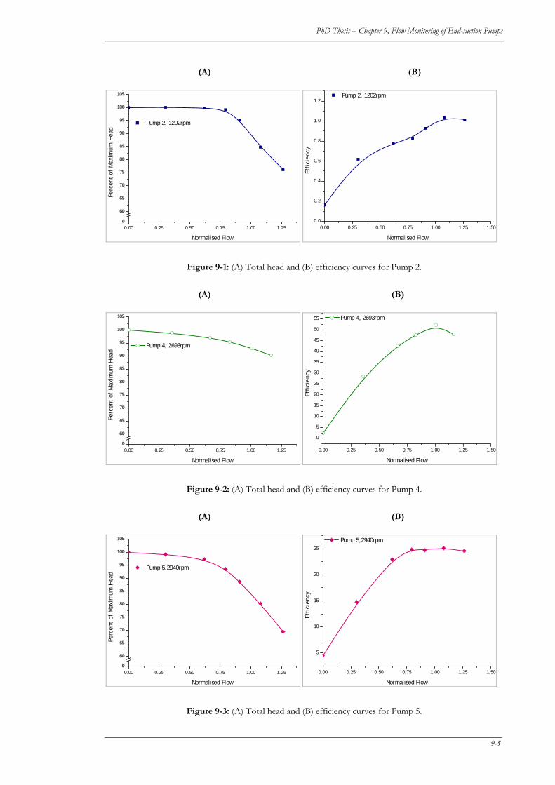
PhD Thesis – Chapter 9, Flow Monitoring of End-suction Pumps
(A) (B)
0.00 0.25 0.50 0.75 1.00 1.250
60
65
70
75
80
85
90
95
100
105
Pump 2, 1202rpm
Perc
ent
of M
axim
um H
ead
Normalised Flow 0.00 0.25 0.50 0.75 1.00 1.25 1.50
0.0
0.2
0.4
0.6
0.8
1.0
1.2 Pump 2, 1202rpm
Effi
cien
cy
Normalised Flow
Figure 9-1: (A) Total head and (B) efficiency curves for Pump 2.
(A) (B)
0.00 0.25 0.50 0.75 1.00 1.250
60
65
70
75
80
85
90
95
100
105
Pump 4, 2693rpm
Perc
ent
of M
axim
um H
ead
Normalised Flow
0.00 0.25 0.50 0.75 1.00 1.25 1.50
0
5
10
15
20
25
30
35
40
45
50
55 Pump 4, 2693rpm
Effi
cien
cy
Normalised Flow
Figure 9-2: (A) Total head and (B) efficiency curves for Pump 4.
(A) (B)
0.00 0.25 0.50 0.75 1.00 1.250
60
65
70
75
80
85
90
95
100
105
Pump 5,2940rpm
Perc
ent
of M
axim
um H
ead
Normalised Flow
0.00 0.25 0.50 0.75 1.00 1.25 1.50
5
10
15
20
25
Pump 5,2940rpm
Effi
cien
cy
Normalised Flow
Figure 9-3: (A) Total head and (B) efficiency curves for Pump 5.
9-5
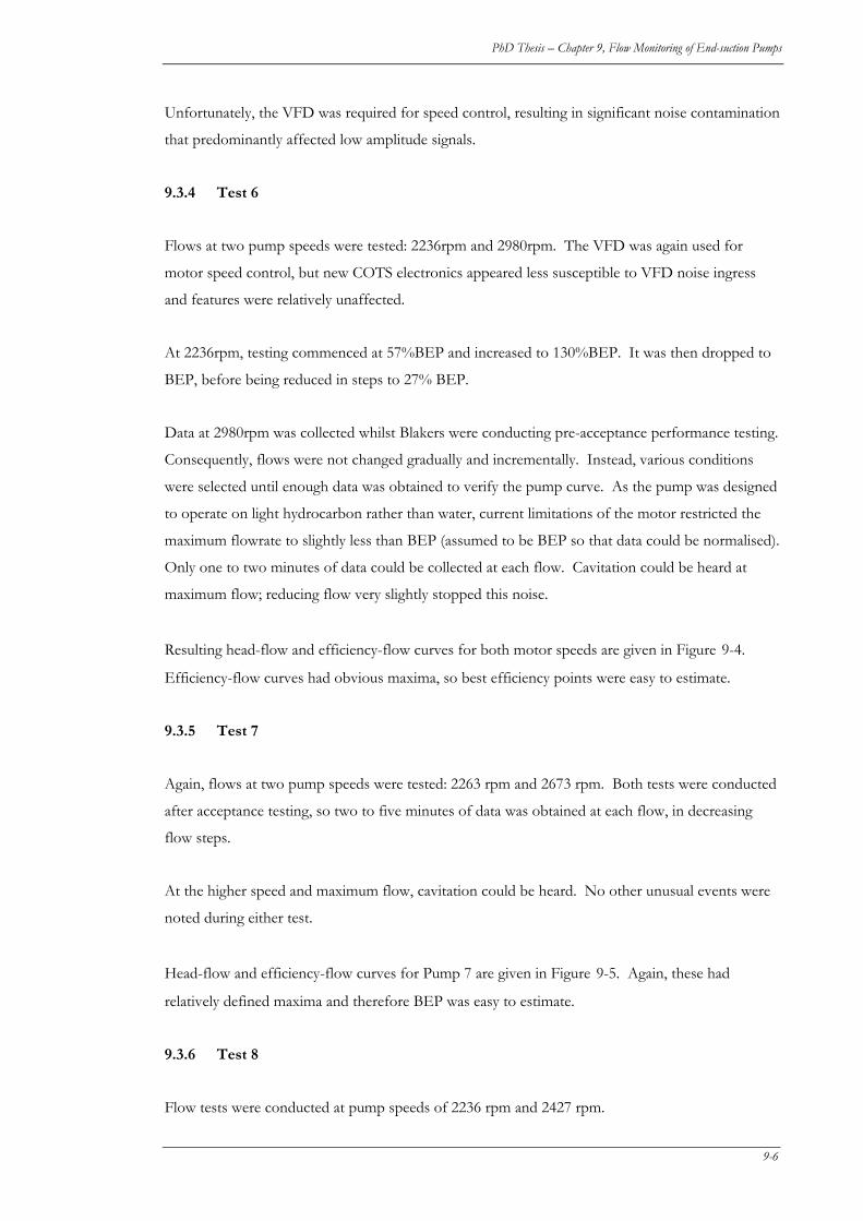
PhD Thesis – Chapter 9, Flow Monitoring of End-suction Pumps
Unfortunately, the VFD was required for speed control, resulting in significant noise contamination
that predominantly affected low amplitude signals.
9.3.4 Test 6
Flows at two pump speeds were tested: 2236rpm and 2980rpm. The VFD was again used for
motor speed control, but new COTS electronics appeared less susceptible to VFD noise ingress
and features were relatively unaffected.
At 2236rpm, testing commenced at 57%BEP and increased to 130%BEP. It was then dropped to
BEP, before being reduced in steps to 27% BEP.
Data at 2980rpm was collected whilst Blakers were conducting pre-acceptance performance testing.
Consequently, flows were not changed gradually and incrementally. Instead, various conditions
were selected until enough data was obtained to verify the pump curve. As the pump was designed
to operate on light hydrocarbon rather than water, current limitations of the motor restricted the
maximum flowrate to slightly less than BEP (assumed to be BEP so that data could be normalised).
Only one to two minutes of data could be collected at each flow. Cavitation could be heard at
maximum flow; reducing flow very slightly stopped this noise.
Resulting head-flow and efficiency-flow curves for both motor speeds are given in Figure 9-4.
Efficiency-flow curves had obvious maxima, so best efficiency points were easy to estimate.
9.3.5 Test 7
Again, flows at two pump speeds were tested: 2263 rpm and 2673 rpm. Both tests were conducted
after acceptance testing, so two to five minutes of data was obtained at each flow, in decreasing
flow steps.
At the higher speed and maximum flow, cavitation could be heard. No other unusual events were
noted during either test.
Head-flow and efficiency-flow curves for Pump 7 are given in Figure 9-5. Again, these had
relatively defined maxima and therefore BEP was easy to estimate.
9.3.6 Test 8
Flow tests were conducted at pump speeds of 2236 rpm and 2427 rpm.
9-6
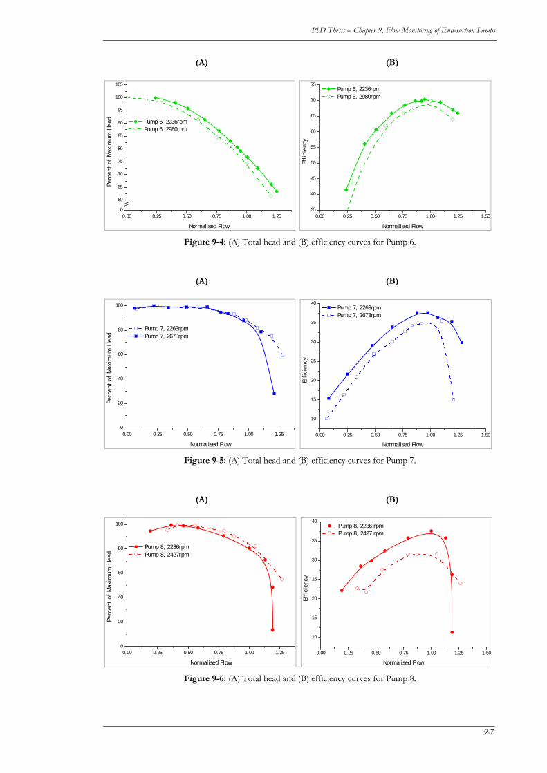
PhD Thesis – Chapter 9, Flow Monitoring of End-suction Pumps
(A) (B)
0.00 0.25 0.50 0.75 1.00 1.250
60
65
70
75
80
85
90
95
100
105
Pump 6, 2236rpm Pump 6, 2980rpm
Perc
ent
of M
axim
um H
ead
Normalised Flow
0.00 0.25 0.50 0.75 1.00 1.25 1.5035
40
45
50
55
60
65
70
75 Pump 6, 2236rpm Pump 6, 2980rpm
Effi
cien
cy
Normalised Flow
Figure 9-4: (A) Total head and (B) efficiency curves for Pump 6.
(A) (B)
0.00 0.25 0.50 0.75 1.00 1.250
20
40
60
80
100
Pump 7, 2263rpm Pump 7, 2673rpm
Perc
ent
of M
axim
um H
ead
Normalised Flow
0.00 0.25 0.50 0.75 1.00 1.25 1.50
10
15
20
25
30
35
40 Pump 7, 2263rpm Pump 7, 2673rpm
Effi
cien
cy
Normalised Flow
Figure 9-5: (A) Total head and (B) efficiency curves for Pump 7.
(A) (B)
0.00 0.25 0.50 0.75 1.00 1.250
20
40
60
80
100
Pump 8, 2236rpm Pump 8, 2427rpm
Perc
ent
of M
axim
um H
ead
Normalised Flow
0.00 0.25 0.50 0.75 1.00 1.25 1.50
10
15
20
25
30
35
40 Pump 8, 2236 rpm Pump 8, 2427 rpm
Effi
cien
cy
Normalised Flow
Figure 9-6: (A) Total head and (B) efficiency curves for Pump 8.
9-7
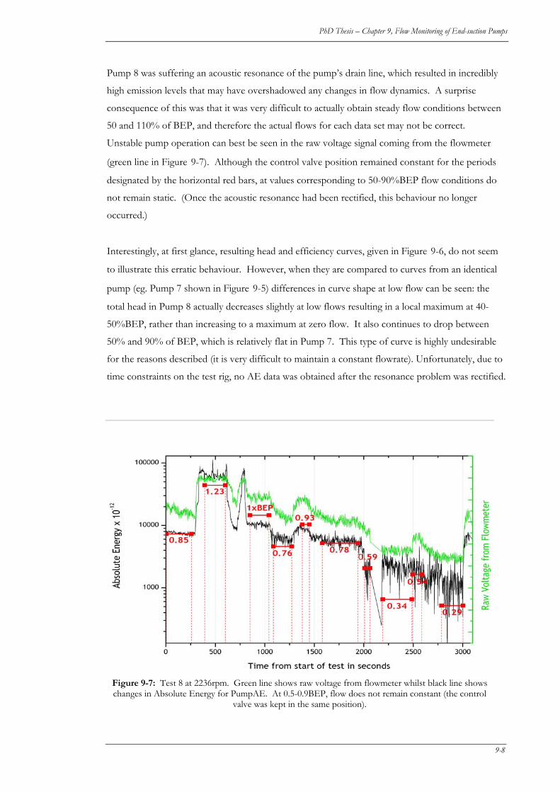
PhD Thesis – Chapter 9, Flow Monitoring of End-suction Pumps
Pump 8 was suffering an acoustic resonance of the pump’s drain line, which resulted in incredibly
high emission levels that may have overshadowed any changes in flow dynamics. A surprise
consequence of this was that it was very difficult to actually obtain steady flow conditions between
50 and 110% of BEP, and therefore the actual flows for each data set may not be correct.
Unstable pump operation can best be seen in the raw voltage signal coming from the flowmeter
(green line in Figure 9-7). Although the control valve position remained constant for the periods
designated by the horizontal red bars, at values corresponding to 50-90%BEP flow conditions do
not remain static. (Once the acoustic resonance had been rectified, this behaviour no longer
occurred.)
Interestingly, at first glance, resulting head and efficiency curves, given in Figure 9-6, do not seem
to illustrate this erratic behaviour. However, when they are compared to curves from an identical
pump (eg. Pump 7 shown in Figure 9-5) differences in curve shape at low flow can be seen: the
total head in Pump 8 actually decreases slightly at low flows resulting in a local maximum at 40-
50%BEP, rather than increasing to a maximum at zero flow. It also continues to drop between
50% and 90% of BEP, which is relatively flat in Pump 7. This type of curve is highly undesirable
for the reasons described (it is very difficult to maintain a constant flowrate). Unfortunately, due to
time constraints on the test rig, no AE data was obtained after the resonance problem was rectified.
Figure 9-7: Test 8 at 2236rpm. Green line shows raw voltage from flowmeter whilst black line shows changes in Absolute Energy for PumpAE. At 0.5-0.9BEP, flow does not remain constant (the control
valve was kept in the same position).
9-8

PhD Thesis – Chapter 9, Flow Monitoring of End-suction Pumps
At high speed (2427rpm) and very low flows (<50% BEP) the discharge hose was seen to “jump
around” and pulsations could be heard emanating from the test rig.
9.4 AE RESULTS
As can be seen in Figure 9-9 and Figure 9-11, PumpAE trends varied widely between pumps.
For data collected from the pump casing, the following features showed the most consistent trends
and tightest confidence limits:
• All RMS and energy features
• Peak amplitudes
• Octave and third-octave band powers, in particular those having centre frequencies
between 256kHz and 512kHz inclusive.
• All wavelet energies
Kurtosis, crest factor, and most hit features (including rise time) displayed no recognisable trends or
had confidence limits that exceeded the trends they encompassed. For brevity, these results are not
included. Swansong filtering or wavelet denoising did not alter results significantly.
Unless otherwise indicated, feature graphs shown can be considered representative of other trends.
9.4.1 Changes at High flow
In all but one test, features increased at flows above BEP (see Figure 9-9 to Figure 9-11),
presumably due to the onset of incipient cavitation. Changes at high flow were evident in virtually
all feature trends and hit contour plots (see Figure 9-8) appeared similar to those presented in
Chapter 7.
In many tests, high flow was also characterised by an increase in the variability of AE Energy
signals, as illustrated in Figure 9-8A: Absolute Energy (the black line) is relatively smooth at low
flows, but becomes less consistent as flow increases above BEP. This would be expected after
commencement of cavitation due to the formation and collapse of vapour bubbles. The changes
are less obvious in Figure 9-8B because Absolute Energy is displayed using a log scale.
9-9
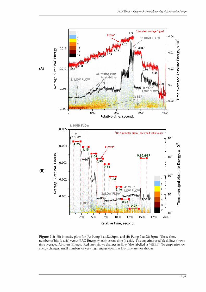
PhD Thesis – Chapter 9, Flow Monitoring of End-suction Pumps
(A)
(B)
Figure 9-8: Hit intensity plots for (A) Pump 6 at 2263rpm, and (B) Pump 7 at 2263rpm. These show number of hits (z axis) versus PAC Energy (y axis) versus time (x axis). The superimposed black lines shows time averaged Absolute Energy. Red lines shows changes in flow (also labelled as %BEP). To emphasise low energy changes, small numbers of very high-energy events at low flow are not shown.
9-10
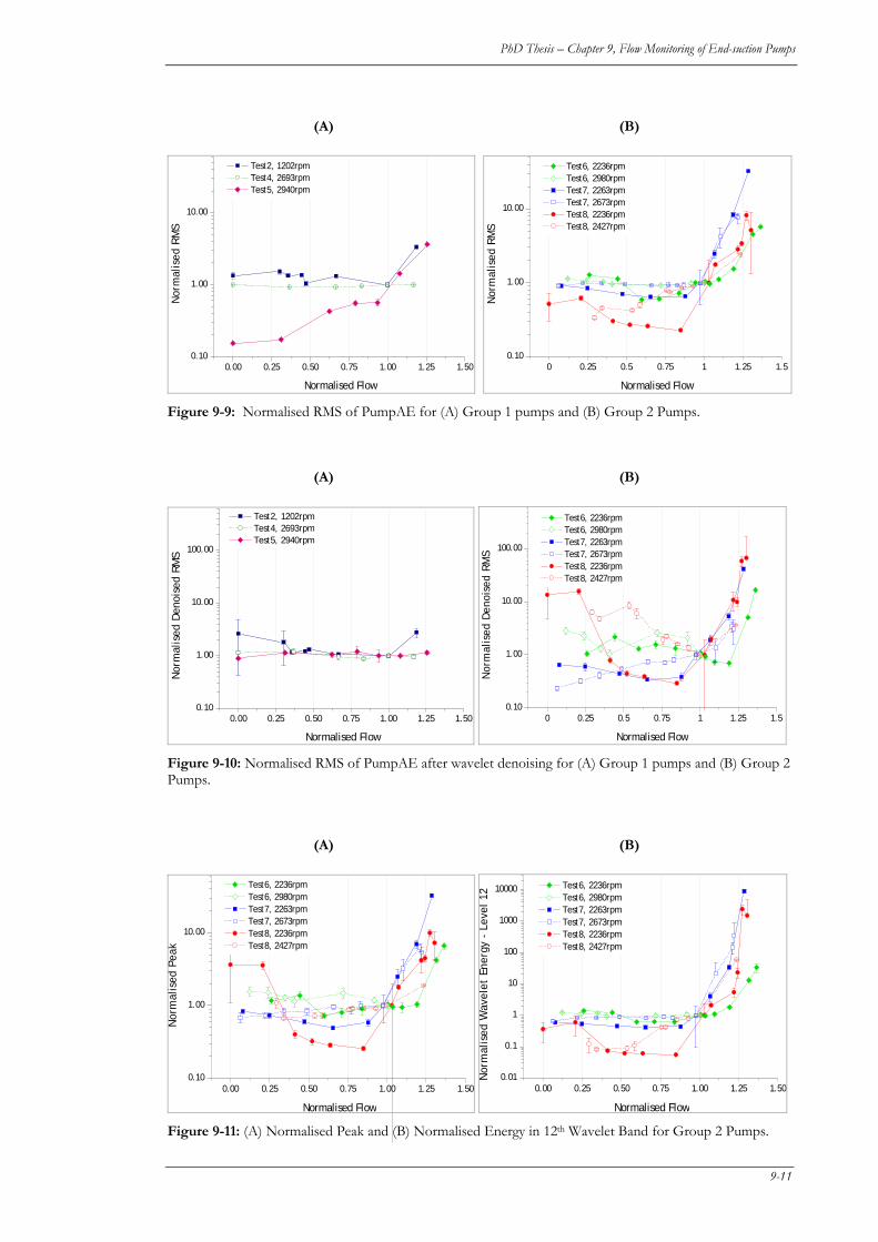
PhD Thesis – Chapter 9, Flow Monitoring of End-suction Pumps
(A) (B)
0.00 0.25 0.50 0.75 1.00 1.25 1.500.10
1.00
10.00
Test2, 1202rpm Test4, 2693rpm Test5, 2940rpm
Nor
mal
ised
RM
S
Normalised Flow 0 0.25 0.5 0.75 1 1.25 1.5
0.10
1.00
10.00
Test6, 2236rpm Test6, 2980rpm Test7, 2263rpm Test7, 2673rpm Test8, 2236rpm Test8, 2427rpm
Nor
mal
ised
RM
S
Normalised Flow Figure 9-9: Normalised RMS of PumpAE for (A) Group 1 pumps and (B) Group 2 Pumps.
(A) (B)
0.00 0.25 0.50 0.75 1.00 1.25 1.500.10
1.00
10.00
100.00
Test2, 1202rpm Test4, 2693rpm Test5, 2940rpm
Normalised Flow
Nor
mal
ised
Den
oise
d RM
S
0 0.25 0.5 0.75 1 1.25 1.5
0.10
1.00
10.00
100.00
Test6, 2236rpm Test6, 2980rpm Test7, 2263rpm Test7, 2673rpm Test8, 2236rpm Test8, 2427rpm
Normalised Flow
Nor
mal
ised
Den
oise
d RM
S
Figure 9-10: Normalised RMS of PumpAE after wavelet denoising for (A) Group 1 pumps and (B) Group 2 Pumps.
(A) (B)
0.00 0.25 0.50 0.75 1.00 1.25 1.500.10
1.00
10.00
Test6, 2236rpm Test6, 2980rpm Test7, 2263rpm Test7, 2673rpm Test8, 2236rpm Test8, 2427rpm
Normalised Flow
Nor
mal
ised
Pea
k
0.00 0.25 0.50 0.75 1.00 1.25 1.50
0.01
0.1
1
10
100
1000
10000 Test6, 2236rpm Test6, 2980rpm Test7, 2263rpm Test7, 2673rpm Test8, 2236rpm Test8, 2427rpm
Normalised Flow
Nor
mal
ised
Wav
elet
Ene
rgy
- Le
vel
12
Figure 9-11: (A) Normalised Peak and (B) Normalised Energy in 12th Wavelet Band for Group 2 Pumps.
9-11
PhD Thesis – Chapter 9, Flow Monitoring of End-suction Pumps
Hit intensity plots (Figure 9-8) also show a sudden drop in the number of very low energy (VLE)
hits as flow rises above BEP, whilst the number and amplitude of large energy hits increase.
9.4.2 Changes at Low Flow
All pumps were designated by HI standards as having ‘Low’ suction energies (listed in Appendix
E). Damaging recirculation and increasing AE levels at low flows were therefore not expected.
Significant variability was observed in all features at flows below BEP, indicating that changes in the
hydrodynamic behaviour at low flow were not consistent. This was supported by qualitative
observations reported at the time of testing, summarised in the section 9.3. As could be expected,
the smoothest trends were obtained (a) for pumps with flat head-flow curves and (b) when a
reasonable amount of data could be acquired at each condition (i.e. Test 7, designated by the blue
lines in Figure 9-9 to Figure 9-11).
Only Pump 8 (suffering from an acoustic resonance problem) showed any increase in parameters at
low flow. This is the most pronounced in the Denoised RMS signal (Figure 9-10B) where results
appear similar to those presented in Chapter 8, increasing at low and high flows. At the lowest
flows AE features dropped and the discharge hose was clearly seen to be pulsating. Thus it is
concluded that this decrease in AE features is probably due to significant low flow recirculation
attenuating acoustic emissions.
Pump 5 had another unexpected trend at low flow. Of all end-suction pumps tested, this had the
highest suction-specific-speed, suction energy (albeit still considered ‘Low’) and suction
recirculation factor, indicating that of any of these six pumps, it would be the most likely to suffer
from recirculation. However, it was also the smallest unit tested so signals might be hard to detect
above the noise floor at low flow. It is also possible, but less likely depending on the volume of
bubbles and exact sensor placement with respect to the location of any recirculation, that
vaporisation could be attenuating signals further.
Conversely, the trend could be genuine. A recent industry publication reported two small pumps
(1x1.5-7 and 3x4-15) for which normalised overall vibration results also had a positive or flat slope
to the left of BEP [89]. The author concluded this was due to the pump’s hydraulic design, but no
further details on the pump were given. He also suggested that the “bathtub” vibration curve
suggested by API 610 [1] (that was seen in AE results presented in Chapter 8), in which overall
levels increase at low and high flows (presumably caused by hydraulic excitations), is not
representative of all pumps. Test 5 results could be viewed as supporting these conclusions.
Further testing is required to identify what types of pumps fall into this category.
9-12
PhD Thesis – Chapter 9, Flow Monitoring of End-suction Pumps
One final observation of AE data at low flows can be derived from the hit-intensity plots given in
Figure 9-8. BEP (Region 3) was characterised by small number of very low energy (VLE) hits
which increased in number but decreased in severity as flow reduced. At very low flows (<50%
BEP) they started to decrease in number and increase in amplitude. Unfortunately, because of their
very small energy, they contributed little to time-averaged AE features, which showed little change
at intermediate flows (eg. Absolute Energy, shown as black lines on Figure 9-8). Averaged trends
were also unaffected. These VLE patterns are much clearer in Pump 6 (Figure 9-8A) than in Pump
7 (Figure 9-8B), which is the larger of the two pumps, and are similar to the results presented in
Chapter 8.
9.4.3 Results at BEP
As already discussed, hit intensity plots (particularly in larger pumps) show a distinct change in the
energy and number of individual AE events at, or around, BEP (Region 3 on Figure 9-8).
Contrary to the reports of others reviewed in the previous chapter, in most pumps tested as part of
this thesis the local minimum (or maximum) in feature curves occurred below BEP. Three reasons
are suggested for these results. Firstly, the location of BEP in many pumps was very difficult to
verify. Secondly, some of these pumps (particularly 2 and 5) were specifically designed for low flow
operation and therefore the point at which the fluid enters the pump with the least shock would be
expected to occur at flows below BEP. Finally, AE features do not discriminate between emission
sources, but rather are an accumulation of all hydrodynamic conditions within the pump.
Therefore, the process of averaging favours sources with larger amplitude emissions, or those
which occur in much greater numbers, than smaller, less numerous events. In small pumps, many
of the relative changes that occur with varying flow rates are subtle, so may be hidden by the
averaging process.
9.4.4 Other observations
It was not uncommon for AE levels to take some time to stabilise, particularly at low or
intermediate flows. This is illustrated in Figure 9-8: at flows between 80 and 96% of BEP, AE
levels (black line) kept increasing for some time after a new flow condition (red line) was
established. It is not as noticeable at flows above BEP, or at very low flows. This tendency was
also much less likely in pumps that have flat head-flow curves, as illustrated in Figure 9-8; when
testing Pump 6, which had a highly sloping head-flow characteristic curve, AE values took much
longer to stabilise (Figure 9-8 A) than when testing Pump 7 (Figure 9-8 B), which had a much
flatter curve.
9-13
PhD Thesis – Chapter 9, Flow Monitoring of End-suction Pumps
9.5 DISCUSSION & CONCLUSIONS
9.5.1 Detection of changes in hydraulic conditions
Some preliminary conclusions about hydraulic conditions in pumps can be derived from the data
presented. High flow conditions above BEP result in an increase in AE energy and amplitude
levels. Signal variability also increases. This supports the work of others, reported in Chapter 8,
which verified that AE levels increase substantially with the onset of incipient cavitation. At high
flows, this condition can be expected and thus it is concluded that the rise in AE features above
BEP is due to this phenomenon.
Although it unlikely that any of the healthy pumps (i.e. except for Pump 8) were suffering from
damaging recirculation due to their low suction energies, some changes in the acoustic emissions
were observed. Hit intensity plots show that low flow conditions, not associated with severe
pulsations, are characterised by a very large number of very small energy events. These decrease in
number and increase in amplitude as flow increases towards BEP. This supports the findings of
the previous chapter. At very low flows, AE hits also increase in energy and decrease in number
but much more rapidly than at flows approaching BEP. High flows, in addition to the reasonable
number of high energy events expected with incipient cavitation, are characterised by very few
small-energy discrete events. Therefore, it is likely that the relative size and energy of an individual
acoustic emission event is related to the size and energy of the originating vapour bubble.
These last observations have not been reported in previous work on AE monitoring of centrifugal
pumps. They also suggest that the best type of feature to identify off-duty conditions may be based
on extracting and quantifying these low energy events. Unfortunately, the extent of these changes
varies substantially with pump size and design and in some cases changes are barely noticeable.
Therefore further development and processing is required to identify how best to quantify and
normalise these low energy changes.
9.5.2 Pump Testing Process
Ordinarily, most of this data would have been omitted from a publication or thesis, justified by
claiming that the experimental procedure was flawed in some way. Instead, “good” results would
be used to illustrate the hypothesis that AE is a useful measure of flow conditions in a pump. As
Chapter 8 showed, there is some evidence to support this argument. However, “good” results are
only part of the story. If, instead, the hypothesis was to determine whether AE could be used by
industry to reliably identify hydraulic conditions in a pump, then it is important to appreciate when
and how such results can, and cannot, be obtained.
9-14
PhD Thesis – Chapter 9, Flow Monitoring of End-suction Pumps
This chapter is therefore included to illustrate two points; firstly, that AE measurements are highly
sensitive to the testing environment and secondly, to propose that actually setting up a pump test to
acquire good AE data is not a simple task. The author suggests that smaller pumps are particularly
sensitive to hydraulic test conditions because acoustic emission energy variations with differing flow
conditions are relatively small. In larger pumps, such as the double suction pump discussed in the
previous chapter, changes in hydraulic conditions are sufficiently large as to (a) have a dominant
hydrodynamic mechanism and (b) swamp the inherent variability of AE signals.
This variability does not affect verification of basic head-flow and efficiency-flow characteristics
used to measure static conditions, such as pressure, flow and motor power because static
transducers are relatively immune to small-scale hydraulic disturbances. Acoustic emission sensors
on the other hand are very sensitive to this variability and therefore to acquire accurate flow-AE
feature curves, it is extremely important to obtain steady-state conditions at each flow tested. If an
extreme condition has been measured (eg. high flow cavitation or low flow recirculation) sufficient
time must be allowed for conditions to stabilise and any vapour bubbles to condense back into
liquid. Pumps must also be free of acoustic or hydraulic problems that could overshadow changes
in flow.
In essence, AE testing must be much slower and more deliberate than during traditional pump
acceptance tests. Only then can the AE analysts and pump owners be comfortable they have
obtained a true indication of the pump’s hydraulic behaviour.
9-15
10. CCOONNCCLLUUSSIIOONNSS &&
RREECCOOMMMMEENNDDAATTIIOONNSS 1100
10.1 DISCUSSION
The biggest challenge of this project was its multi-disciplinary nature. To develop a feasible seal or
pump monitoring solution based on AE requires knowledge not only of acoustic emission, pumps,
seals and their hydro-mechanical failure mechanisms, but also of computing, electronics design,
advanced signal processing, fluid dynamics and structural mechanics.
Although any final system developed for monitoring mechanical seals and/or hydraulic conditions
in industrial centrifugal pumps needs to be small, mobile and cost effective, the requirements of
such a system must first be established. This necessitated collecting data with more flexible (and
less mobile) equipment that could monitor a large number of parameters; the most suitable features
for early warning of incipient failures could then be determined.
As AE hardware was not initially available, a review of alternative systems then on the market for
monitoring acoustic emissions from machine components was conducted, based on their
underlying research and patents. The aim of this work was to: (a) determine whether purchasing
existing equipment for monitoring failures in seals and pumps was appropriate, (b) identify the
similarities and/or differences in these technologies so that a base set of requirements for in-house
electronics could be developed and (c) establish whether results of these different systems were
directly comparable. This work was presented at ICOMS in 2003 and is included as Chapter 2 of
this thesis.
From the perspective of this research project the results of the review were disheartening. Firstly, it
determined that although each manufacturer effectively measured some form of acoustic emission
10-1

PhD Thesis – Chapter 10, Conclusions & Recommendations
signal, each coined their own name for the stress wave or resulting output. Secondly, an analysis of
the signal processing techniques underpinning these systems determined that enough disparity
between variants, in sensor type, signal condition performed and output algorithms, precluded their
direct comparison. Furthermore, no one system was obviously superior to any other. Thirdly,
only one of the products considered was flexible enough to monitor different types of failure from
those for which it was originally designed (and in 2002 that option was still unavailable in Australia);
the remainder were specifically geared to detect one particular fault type (usually rolling element
bearing problems), and although the marketing literature stated they could were more generic, there
was little evidence to support these claims. Most systems were also not suitable for continuous on-
line monitoring.
For these various reasons, the author decided that the most appropriate option for this research
project was to develop a system in-house. This would allow generic signal processing techniques to
be used, with methods and results being expressed in well-understood terminology.
The final in-house system used commercially available AE sensors and preamplifiers, generic data
acquisition hardware, custom built filters and amplifiers, and software programs written by the
author in LabVIEW. The greatest limitation of this system was insufficient immunity against noise
emanating from variable frequency drives, inadequate hit capturing capability and the inability to
collect information prior to event triggering. Consequently, when commercial-grade equipment
was made available, this in-house system was forsaken9. Interestingly, although the new COTS
hardware did provide improved noise immunity, VFD interference still remains a problem at low
signal levels.
A pump-rig was also designed and constructed at UWA in order to collect experimental data from
mechanical seal failures under controlled conditions. Space and budget restrictions limited the size
of the facility and pump. This ultimately ensured that modern, well-designed mechanical seals
installed therein survived all punishment the author could inflict, including: heating the seal
chamber jacket to 130 degrees Celsius, cavitating the pump by throttling the suction valve, running
the seal completely dry for several days and injecting ceramic oxide particles into the seal chamber
via the flush. With the help of the seal manufacturer, it was determined that the pump was simply
too small and slow to generate conditions that would exceed the actual (rather than published)
design limits of typical mechanical seals. Some preliminary findings were published in [106], an
extract from which is included in Appendix F.
9 Work has continued by the designer, Mr Paul Kelly, with the aim of ultimately providing a cost-effective
electronics platform for any seal and pump AE monitoring algorithms developed by the author.
10-2
PhD Thesis – Chapter 10, Conclusions & Recommendations
Despite the inability to initiate seal failures, the process was useful for identifying a number of other
issues that needed to be resolved before seal failure signals could be correctly interpreted and
actioned. These were listed in the introduction and how this thesis addressed these problems are
hereby summarised.
(a) Commercially available AE systems have been designed for structural monitoring
applications (eg. pressure vessels, cranes etc). AE signals from pumps are very
different and so traditional AE signal-processing techniques may need to be
supplemented and/or modified to ensure that they accurately characterise changes in
machinery AE signals.
AE signals in pumps are comprised of impulsive and continuous emissions. Depending on the
nature of the problem, traditional AE applications generally focus on one or other signal form.
Crack monitoring for example, is concerned with discrete events, whilst leak detection seeks
continuous emission signals. Rotating machines, such as centrifugal pumps, have a variety of
failure mechanisms or failure inducing hydrodynamic conditions, each comprising of differing
amounts of burst and continuous emissions.
COTS AE systems are primarily designed for structural monitoring and therefore have significant
capacity to acquire, characterise and store information pertaining to discrete AE events.
Unfortunately, as already mentioned, their capability to monitor continuous AE signals over
extended periods of time is limited. Therefore, to supplement the features available, time
waveforms were collected and subjected to further analysis. Additional signal descriptors, as
outlined in Chapter 3, were selected for their accepted suitability to vibration analysis of rotating
machinery signals. These included statistical variables, frequency octave-band energies and discrete
wavelet energies. As longer waveforms were required to overcome the inherent non-stationarity of
AE signals, processing algorithms to calculate these additional features from shorter subsets of the
signal were also devised by the author. In total, for all data collected from centrifugal pumps, 42
features were calculated (or extracted from COTS system data files) and logged.
Structural AE work, and the COTS systems developed for them, generally display test results
graphically. This is acceptable when analysing data from a time-limited test and when acceptance
criteria are known in advance. However, when new applications for extended monitoring are being
developed, some way of assimilating the data is required so that the acceptance criteria can be
established. To do this, ensemble averages with 90% confidence limits were calculated for all 42
features. As shown in chapters 8 and 9, this can be a very effective mechanism for detecting and
comparing trends but is not widely used by the AE community. This is probably because digesting
10-3
PhD Thesis – Chapter 10, Conclusions & Recommendations
data in this way is not possible when relying solely on functionality built into vendor supplied
software packages.
(b) A variety of noise sources, peculiar to machinery monitoring applications, can appear
very similar to acoustic emission sources, and if not identified and removed will, at
best, lead to confusion when interpreting results or at worst, result in a perfectly healthy
seal or pump being removed from service.
Acoustic emission signals are very small (in the order of a few microvolts to a few millivolts).
Although amplifiers are used to increase the size of the signals throughout the measurement chain,
signals are still very sensitive to noise contamination. As frequencies get higher, amplitudes tend to
decrease and vulnerability to noise contamination increases. Furthermore, certain types of noise
only become problematic at higher frequencies. AE signals from rotating machines are even more
at risk because they are often collected using broadband non-resonant sensors measuring signals up
to 1-2MHz. Consequently, noise identification, management and mitigation needs to be very
carefully considered.
Problems are compounded when machinery is driven by variable frequency drives. These control
the speed of a motor by changing the voltage frequency. Unfortunately, they emit pulses of
broadband, high frequency electro-magnetic radiation. This couples to the equipment or AE
instrumentation resulting in very large, broadband, impulsive noise bursts superimposed onto AE
signals at a switching frequency of 10-50kHz. Noise bursts appear very similar to genuine acoustic
emissions, particularly when viewed in isolation (i.e. hit data) and are captured by AE
instrumentation as if they were genuine AE hits.
Furthermore, hydro-mechanical machines such as centrifugal pumps have a number of genuine
mechanisms that generate acoustic emissions. Some of these ultimately lead to failure, whilst others
are of little consequence and can probably be ignored. Therefore an important part of any fault
identification process is separating wanted from unwanted signals.
Chapter 4 reviewed a number of denoising techniques for identifying noise in AE signals at the
time of data collection, or removing the effects thereafter. Examples based on actual AE signals
collected from centrifugal pumps by the author, were given to demonstrate how each could be used
to improve legitimacy of analysed data. Although none of these techniques were new, in the case
of Swansong filtering and averaging, their application to noise management of machinery AE had
not been reported previously. Discrete wavelet analysis is a widely applied denoising technique, but
recommendations on how best to apply it to AE machinery monitoring could not be found. As a
result, the author spent considerable time and effort evaluating different processing options before
10-4

PhD Thesis – Chapter 10, Conclusions & Recommendations
determining the best set of parameters. To simplify this process for others, the author’s
experiences are collated into a set of guidelines and recommendations included in this chapter. In
essence, Haar wavelets were found to be the most effective at removing background noise whilst
retaining individual events. Improved performance was obtained when threshold values were
determined individually for every level, and when digital filters were not applied. Energy in the
background and retained signals was quantified separately and treated as additional AE features that
related to the continuous and discrete parts of the signal respectively.
All techniques included in Chapter 4 were used to successfully identify or denoise signals collected
in later chapters. As shown in Chapter 8, Swansong filtering and wavelet denoising can improve
the extraction of trends that are otherwise swamped by noise. Unfortunately, no method tested
was found to reduce the effects of VFD contamination. Work in reducing the susceptibility of AE
instrumentation to VFD noise ingress is therefore required.
(c) As the time of failure is unpredictable, the amount of data that can be collected is
considerable. Furthermore, given that the ultimate aim is to detect incipient failure, all
of this data needs to be analysed and scrutinised. To do this manually would be
impractical.
Continuous pump monitoring resulted in 2-3GB of waveform and feature data every day. This
volume of information could not be analysed manually. Very quickly, even accompanying process
data and experimental conditions became difficult to track. Further complicating analysis, COTS
equipment stored its data in proprietary files that could not be read on a second computer without
purchasing additional software licences.
Although databases are a ubiquitous part of commercial life, for some reason they are not often
used to manage engineering research data. With the help of a systems architect, a database
management system was designed and implemented to manage metadata about AE tests, extract
features from proprietary COTS systems, analyse waveform data as per the algorithms described in
previous chapters and store results in a minable format. Originally devised as an Access database, it
very quickly exceeded that software’s capacity (about 2 million rows in any one table) and was
upgraded to a SQL Server system, with a Microsoft Access user interface. A paper was published
in the Journal of Mechanical Systems and Signal Processing regarding the development of this
database management system and is included as Chapter 5.
The biggest impact of the database management system on this research project was the ease with
which new processing algorithms could be trialled on any data collected and results incorporated
into the database. As soon as a new technique was developed (in any software language) and
10-5

PhD Thesis – Chapter 10, Conclusions & Recommendations
compiled into an appropriate format, data was selected and automated processing commenced.
Results were automatically logged into the database, eliminating errors associated with manually
entering data into spreadsheets or tables. Depending on the nature of the analysis algorithms, up to
20GB of data could be processed in one day, limited primarily by the low cost processing and SQL
server hardware being used.
Another advantage of this system was that it offered huge flexibility in the selection of methods for
analysing, processing and presenting data. Graphs could be displayed using scientific graphing
packages such as Origin or SigmaPlot and signal processing could be performed using the
mathematical platform of choice (which in the author’s case was generally LabVIEW). When speed
or access to system function calls necessitated using lower level languages such as C++, these too
could be seamlessly incorporated into the system. Tools were used for the purpose they were
designed, improving functionality, increasing reliability, decreasing frustration and increasing the
proportion of time that was spent developing new analysis techniques and looking for trends and
patterns in the data.
Managing and maintaining the system, which by the end of this research project comprised of
tables with over 50 million rows, was no longer an onerous task. Archiving and backing-up became
straightforward. If no new analysis techniques were required, analysed raw data could be
permanently archived to optical disk; all interaction with the data now occurred via the database.
With this system, between 250 and 300 Gigabytes of raw AE data was extracted, analysed and
logged during the course of this research project (most of it relating to continuous mechanical seal
operation). The database itself is now over 11GB in size. Yet extracting pertinent results, even for
tests that were processed years ago, is a trivial process.
Whether data is collected by a single researcher in a university using a COTS AE system, or from a
collection of black boxes remotely transmitting extracted features from the field, this type of
database management system will ensure maximum information is extracted from any data
collected. Collectively, this data then becomes the basis for the next generation of expert-based
diagnosis systems.
(d) When it is not possible to locate a sensor where desired, waveguides can be used. The
effect of waveguide shape and material composition needs to be understood so that
signals can be interpreted correctly.
Mechanical seals are contained within a housing (generally referred to as a stuffing box) that is
incorporated into the pump. Acoustic emission generated by the seals must therefore travel via a
10-6

PhD Thesis – Chapter 10, Conclusions & Recommendations
convoluted path to reach a sensor mounted on the stuffing box or pump casing. Alternatively, a
waveguide can be mounted through the stuffing box to the seal, giving signals a more direct
transmission path to the sensor. Waveguides are also useful when pumps contain very hot fluid
(e.g. bitumen pumps) as direct contact with a hot casing could damage AE sensors.
In Chapters 6 and 7, the effects of different waveguide dimensions, material compositions and face
angles were analysed on the temporal and frequency characteristics of simulated AE signals. Prior
research in this area is limited and relates solely to flat-faced, much longer, metallic guides.
Techniques used for analysis included basic feature comparisons, frequency averaging, short-time-
frequency analysis and continuous wavelet transformation. The latter two techniques also
facilitated basic modal analysis.
The work described in chapters 6 and 7 was published as two papers in the Journal of Acoustic
Emission and determined that in the case of short rods, with dimensions of the same order as the
AE wavelengths, signals received by the sensor were affected significantly by the natural
longitudinal frequency of the rod. This was particularly problematic in metallic guides (Mild steel,
SS316 and Aluminium) where strong resonant frequencies dominated responses; effects increased
with length and diameter. Whilst Alumina Oxide ceramic and Delrin rods attenuated signals
significantly, resonant effects were also minimised.
In addition to strongly attenuating signals, pointed metal guides (as opposed to flat faces with
adequate couplant) acted as a bandpass filter, whilst retaining or amplifying the undesirable
harmonic artefacts in the pass band. The amount of attenuation increased with the sharpness of
the point, explaining why previous reports disagreed on the amount of attenuation (if any) imposed
by using a pointed guide. Angled waveguides increased the spectral and modal complexity of
responses, probably due to the excitation of bending modes.
These findings indicate that short, cylindrical, solid waveguides should be avoided if at all possible.
Where absolutely necessary, rods should be as narrow and short as possible, made from very high
acoustic speed materials with inherent damping (i.e. ceramics) and have flat ends attached with a
good couplant.
(e) Acoustic emissions collected from the seal are strongly influenced by the hydraulic
conditions within the pump, and therefore to be able to differentiate between incipient
seal failure and an unfavourable hydraulic condition, the latter must be identified. To
do this, a pump’s individual acoustic emission signature needs to be characterised.
10-7

PhD Thesis – Chapter 10, Conclusions & Recommendations
Although seal failures could not be invoked, observations during extended pump and seal
monitoring indicated that seal AE signals were strongly affected by the hydraulic conditions within
the pump. This, in turn, was affected by how far the pump operated away from its best efficiency
point. It is also well known that suboptimal pump operation affects mechanical seal longevity.
Consequently, it is crucial for any automated seal monitoring device to know where a pump is
operating on its curve so that it can: (a) identify conditions that lead to poor seal reliability and (b)
differentiate between AE signals caused by incipient failure and signals caused by inappropriate
operation.
To determine how AE is affected by moving away from best efficiency point, AE data was
collected from a large double suction pump and a number of new small single suction pumps at a
pump supplier’s test facility. Data was analysed using the processing techniques described in
Chapters 3 and 4 and managed by the system described in Chapter 5.
This work determined that energy features showed the most consistent trends, with tightest
confidence limits. In a large double-suction pump, denoising hit data with a Swansong filter and
waveform data with discrete wavelets improved trends significantly. These techniques were less
successful in smaller pumps for reasons that are described below. Octave-band and wavelet-band
energies showed similar trends to overall energies. Differences between bands were very subtle, if
any.
From the data it can be concluded that average features increase (normalised with respect to the
mean level at BEP) in magnitude above BEP due to the onset of incipient cavitation. Once severe
cavitation is established, AE levels drop. This supports the findings of previous work by others.
Average feature trends below BEP differ substantially between pumps. In the small end-suction
pumps, levels at low flows increased only slightly, from a minima between 0.6 and 0.9BEP, whilst
in one case levels actually decreased. In the much larger, and higher energy double-suction pump,
with a known tendency towards recirculation, features increased substantially at low flows. This
suggests that recirculation can increase AE levels, but probably only in high-energy pumps. More
testing on larger pumps is required to confirm this conclusion.
In addition to averaged feature trends, hit intensity plots were also analysed. These provided
additional information not obvious from in any of the 42 averaged features trended. Flows above
BEP are characterised by a large spread in the energies of individual hits. Flows below BEP on the
other hand, are typified by a very large number of very low energy (VLE) events. These increase in
number, but decrease in amplitude as flow reduces, until at very low flows (<50%BEP) the reverse
trend starts to occur (VLE hits decrease in number and increase in magnitude). This observation
has not been reported elsewhere and may be related to the formation of small recirculation vortices.
10-8
PhD Thesis – Chapter 10, Conclusions & Recommendations
It is hypothesized that at very low flows, these consolidate, grow and collapse due to the varying
pressure distributions within the pump, releasing shock waves that emanate as much larger acoustic
emission events. Preliminary results indicate that in small, low energy pumps, these pulsations are
too small to affect overall signal features, whilst in larger pumps features increase substantially.
More testing is required to determine how pumps can be grouped by their AE-flow characteristics;
this would facilitate more definite conclusions about the causal mechanisms for AE within
centrifugal pumps, particularly at low flows.
Although denoising techniques, trialled as part of this thesis, seem to be very effective at separating
out discrete events in large pumps, they appear ineffective for small pumps. This is probably
because both techniques use fixed criteria for accepting or rejecting hits. As pumps reduce in size,
the amplitude and energy of these events decrease. Based on these observations, a variable filter
will be developed in follow-up work for separating out these events. It is hypothesized that this
filter would provide better identification of low flow in pumps than the AE features trialled to date.
Another conclusion derived from testing is that AE results are much more sensitive to test
condition stability than traditional condition monitoring parameters. Although accurate head-curve
and efficiency-curve data can be obtained from a relatively speedy testing process, AE results
require significantly more care and thus, more time. Flows need to be increased or decreased in
steps, from one extreme to the other so that conditions within the pump change gradually. This
reduces the time for AE levels to stabilise. Larger pumps with steep head-flow curves also take
longer to stabilise because small changes in flow result in larger deviations in the hydrodynamic
pressure field. In retrospect, these observations seem obvious given the known sensitivity of AE
to bubble dynamics, however its effect on the quality of pump test results has not been reported
previously.
Significantly more test work is required to be confident in the conclusions pertaining to
relationships between acoustic emission features and hydraulic conditions in centrifugal pumps.
However, with the systems established as part of this project and issues already overcome, acquiring
and processing this data is limited only by ready access to large numbers of variable size pumps and
the time to collect accurate AE data.
Finally, brevity dictates that some research has been omitted from this final thesis. Work
undertaken in areas of noise identification and mitigation, analysis of cavitation data and
relationships between acoustic emission features and mechanical seal operation is incomplete and
therefore has been omitted. This research is continuing and will be the subject of future
publications.
10-9

PhD Thesis – Chapter 10, Conclusions & Recommendations
10.2 SUMMARY OF FINDINGS
Although the conclusions of this research were detailed in the previous section, the major findings
can be summarised by the following key points:
(1) Vibration monitoring techniques are well suited to analysing acoustic emission waveforms.
(2) Current AE hardware does not provide sufficient noise immunity against interference from
variable frequency drives. This can not be removed during post-processing as signals have
very similar characteristics to genuine AE events.
(3) Denoising techniques, such as wavelets (with Haar wavelets) for waveform data and
Swansong filtering for hit features, are very effective at dividing mixed-mode acoustic
emission signals into discrete and continuous parts.
(4) Database systems simplify the process of trialling new analysis techniques and collating or
interrogating results independently of software and hardware used to collect the data.
When applied to AE monitoring, database servers should be used as the amount of
information will very quickly exceed the limits of desktop database software.
(5) Cylindrical waveguides with dimensions in the same order as the acoustic wavelengths
should be avoided for acoustic emission work, particular when waveform fidelity is
required. If absolutely necessary, rods should be as narrow and short as possible, made
from ceramic material, with flat ends and attached with a good couplant.
(6) Acoustic emission analysis appears very effective at identifying changes in hydraulic
conditions within large centrifugal pumps. Energy features show the most consistent
trends. Overall energy features are much less consistent in smaller pumps, particularly at
low flows.
(7) By measuring AE signals from both the suction and discharge flanges of a pump
simultaneously, automating the process of flow identification in large pumps should be
possible using energy features from both sensors.
(8) Hit energy is a better indicator of hydraulic conditions in small pumps; distinct changes
occur in the distributions of very low energy events with changing flow. Similar patterns
are also observed in large pumps.
10-10

PhD Thesis – Chapter 10, Conclusions & Recommendations
(9) Although this work was applied to a particular type of rotating machine, and in fact
originally a particular component, the approaches described herein can be applied to
continuous monitoring of any rotating or reciprocating machine.
10.3 RECOMMENDATIONS FOR FUTURE WORK
As has already been mentioned, this work is by no means over. The following issues still need to
be resolved before a system for detecting incipient failure of mechanical seals in centrifugal pumps
can be developed:
(1) Improve instrumentation immunity against VFD noise, or develop denoising techniques
that can subsequently remove data coinciding with the drive’s switching frequency from
the analysis dataset;
(2) Design a filter to quantify the magnitude and severity of VSE events typical of low flow
conditions;
(3) Benchmark a large number of new pumps to determine if these can be categorised by the
acoustic emission signature;
(4) Determine how acoustic emission signatures change as a pump deteriorates with age;
(5) Develop a system for failing seals in realistic and controlled conditions so that acoustic
emission data can be collected prior to failure. (A reasonably large pumping system,
running at high speed, should be used to increase the likelihood of success. Working with
mechanical seal manufacturers at their facilities may also increase the chance of obtaining
useful and interpretable incipient failure data.)
(6) Develop small, portable and cheap electronics design that can be permanently installed on
pumps to monitor changes in flow and acoustic emission during life. Current COTS AE
systems are far too large, not particularly portable and prohibitively expensive.
10.4 FINAL WORDS
Ironically, the ultimate goal for maintenance professionals is to make themselves redundant, by
improving equipment reliability and eliminating the need for maintenance all together. Realistically
(and fortunately for those of us at the start of our maintenance careers), that is highly unlikely to be
realised in the foreseeable future. The next best thing is to know exactly how and when equipment
10-11

PhD Thesis – Chapter 10, Conclusions & Recommendations
will fail so that its operational and economic impact can be minimised, or even mitigated
completely.
I started this PhD with the aim of developing such a system for mechanical seals. Despite not
achieving this objective, I am satisfied with progress that has been made. With future input from
pump and seal manufacturers, it is only a matter of time before such a system can be and will be
developed. With the added ability to assess how a pump is performing, my maintenance colleagues
and I may also be able to improve the efficiency of our processing plants and reduce our electricity
demands; this not only returns an economic benefit to our employers but also reduces the damage
these plants inflict on our environment. We can then spend time pondering other obstacles to our
early retirement.
10-12
11. RREEFFEERREENNCCEESS
1111 1. (1995) "API 610 - 1995: Centrifugal Pumps for Petroleum, Heavy Duty Chemical and Gas Industry
Services", 8th ed: American Petroleum Institute.
2. (1995) "Application Note CM3014: What are Enveloping and SEETM?" SKF Condition
Monitoring, pp.1.
3. (1996) "Application Note CM3020: Taking and Interpreting SEETM Pen Readings", SKF
Condition Monitoring, pp.1.
4. (2002) "SWANTM Technology Overview", SWANTECH LLC, pp.1-5.
5. (2003) "PCI-2 Based AE System User's Manual, Part # 6301-1000", Princeton Junction NJ:
Physical Acoustics Corporation.
6. (2003) "PCI-2 Product Bulletin 102803", Physical Acoustics Corporation: Princeton Junction
NJ, pp.1-4.
7. Abbot, P.A. (1989) "Cavitation detection measurements on Francis and Kaplan hydroturbines" in
Proceedings of the ASME Proceedings of International Symposium on Cavitation and
Noise Erosion in Fluids Systems: ASME-Fluids Engineering Division, pp.55-61.
8. Alfayez, L., Mba, D. and Dyson, G. (2005) "The application of Acoustic Emission for detecting
incipient cavitation and the best efficiency point of a 60KW centrifugal pump; case study", NDT&E. In
press.
11-1
PhD Thesis – Chapter 11, References
9. Alfredson, R.J. and Mathew, J. (1985) "Time domain methods for monitoring the condition of rolling
element bearings", Mechanical Engineering Transactions, IEAust: pp.102-107.
10. Amaya, M. (1994) "Recent applications of acoustic emission testing for plant equipments" in
Proceedings of the Progress in Acoustic Emission, VII: Proceedings of the 12th
International Acoustic Emission Symposium, Sapporo, Japan, pp.305-312.
11. Bansal, V., Gupta, B.C., Prakash, A. and Eshwar, V.A. (1990) "Quality inspection of rolling
element bearings using acoustic emission technique", Journal of Acoustic Emission, 9(2): pp.142-
146.
12. Beattie, A.G. (1983) "Acoustic Emission, principles and instrumentation", Journal of Acoustic
Emission, 2(1): pp.95-127.
13. Bendat, J.S. and Piersol, A.G. (2000) "Random Data - Analysis and Measurement Procedures",
3rd. Edition ed, New York: John Wiley & Sons.
14. Bloch, H.P. (1978) "Acoustic incipient failure detection systems are successful at Exxon", The Oil
and Gas Journal, Feb. 6: pp.66-72.
15. Board, D.B. (2000) "Stress Wave Analysis of Turbine Engine Faults" in Proceedings of the
IEEE Aerospace Conference, Big Sky, MT, pp.79-94.
16. Board, D.B. (2002) "Stress Wave Analysis: Presentation to the Vibration Institute" [online], Ed.
Available from: [Accessed: 20/02/2003].
17. Boness, R.J. and McBride, S.L. (1991) "Adhesive and abrasive wear studies using acoustic emission
techniques", Wear, 149: pp.41-53.
18. Boness, R.J., McBride, S.L. and Sobczyk, M. (1990) "Wear studies using acoustic emission
techniques", Tribology International, 23(5): pp.291-295.
19. Brownell, R.B., Flack, R.D. and Kostrewsky, G.J. (1985) "Flow visualisation in the tongue region
of a centrifugal pump", The Journal of Thermal Engineering, 4(2): pp.35-45.
20. Budris, A.R. (1993) "The shortcomings of using pump suction specific speed alone to avoid suction
recirculation problems" in Proceedings of the 10th International Pump Users Symposium,
Texas A&M University.
21. Buzzacchi, G., Cartoceti, M., De Mechelis, C. and Sala, C. (1983) "In-field experience in
condition monitoring of rotating machinery by demodulated resonance analysis", Journal of Acoustic
Emission, 2(1): pp.11-18.
11-2
PhD Thesis – Chapter 11, References
22. Carletona, C.J., Dahlgrena, R.A. and Tate, K.W. (2004) "A relational database for the monitoring
and analysis of watershed hydrologic functions: I. Database design and pertinent queries", Computers &
Geosciences. In press.
23. Carletona, C.J., Dahlgrena, R.A. and Tate, K.W. (2005) "A relational database for the monitoring
and analysis of watershed hydrologic functions: II. Data manipulation and retrieval programs",
Computers & Geosciences. In press.
24. Catlin, J.B.J. (1983) "The use of ultrasonic diagnostic techniques to detect rolling element bearing defects"
in Proceedings of the Machinery Vibration Monitoring and Analysis Meeting, pp.123-130.
25. Cempel, C. (1991) "Vibroacoustic condition monitoring", 1st ed, England: Ellis Horwood Ltd.
26. Cheeke, J.D.N. (2002) "Fundamentals and Applications of Ultrasonic Waves", Boca Raton,
Florida: CRC Press.
27. Chu, S., Dong, R. and Katz, J. (1995) "Relationship between unsteady flow, pressure fluctuations and
noise in a centrifugal pump - Part B: Effects of blade-tongue interactions", ASME Journal of Fluids
Engineering, 117: pp.30-35.
28. Cudina, M. (2003) "Detection of cavitation phenomenon in a centrifugal pump using audible sound",
Mechanical Systems and Signal Processing, 17(6): pp.1335-1347.
29. Derakhshan, O., Houghton, J.R., Jones, R.K. and March, P.A. (1991) "Cavitation monitoring
of hydroturbines with RMS acoustic emission measurement", ASTM STP 1077: pp.305-315.
30. Donoho, D.L. and Johnstone, I. (1995) "Adapting to unknown smoothness via wavelet shrinkage",
Journal of the American Statistical Association, 90: pp.1200-1224.
31. Dupont "Delrin Design Guide - Module III" [online], Ed. Available from:
http://plastics.dupont.com/plastics/pdflit/americas/delrin/230323c.pdf [Accessed:
15.03.2004].
32. Dvoracek, J., Petras, J. and Pazdera, L. (2000) "The phase of contact damage and its description by
help of acoustic emission", Journal of Acoustic Emission, 18: pp.81-86.
33. ETSU and AEAT PLC (2001) "Study on improving the energy efficiency of pumps", European
Commission, pp.70.
34. Finley, R.W. (1980) "Computerized preventative maintenance systems using modified acoustic emission
techniques", Materials Evaluation, 38: pp.15-20.
11-3
PhD Thesis – Chapter 11, References
35. Fowler, T.J. (1993) "Structural integrity testing of process piping with acoustic emission" in
Proceedings of the 1st International Symposium of Process Industry Piping, Orlando,
Florida: National Association of Corrosion Engineers.
36. Fowler, T.J., Blessing, J.A., Conslisk, P.J. and Swanson, T.L. (1989) "The MONPAC system",
Journal of Acoustic Emission, 8(3).
37. Fraser, W.H. (1981) "Flow recirculation in centrifugal pumps" in Proceedings of the 10th Annual
Turbomachinery Symposium, Texas, USA: Turbomachinery Laboratory, Texas A&M
University, pp.95-100.
38. Ganesan, R., Das, T.K., Sikder, A.K. and Kumar, A. (2003) "Wavelet based identification of
delamination defect in CMP (Cu-Low k) Using Nonstationary acoustic emission signal", IEEE
Transactions on Semiconductor manufacturing, 16(4): pp.677-685.
39. Graff, K.F. (1975) "Wave motion in elastic solids", London: Oxford University Press.
40. Grosse, C., Finck, F., Kurz, J. and Reinhardt, H.W. (2004) "Improvement of AE technique using
wavelet algorithms, coherence functions and automatic data analysis", Construction and Building
Materials, 18: pp.203-213.
41. Guelich, J.F. and Bolleter, U. (1992) "Pressure Pulsations in Centrifugal Pumps", ASME Journal
of Vibration and Acoustics, 114: pp.272-279.
42. Guelich, J.F., Schwarz, D. and Carney, B. (1990) "Pump vibrations caused by cavitation" in
Proceedings of the Institution of Mechanical Engineers, Fourth European Congress, Fluid
Machinery for the Oil, Petrochemical and related industries, pp.55-60.
43. Hamstad, M.A., Downs, K.S. and O’Gallagher, A. (2003) "Practical Aspects of Acoustic
Emission Source Location by a Wavelet Transform", Journal of Acoustic Emission. "Practical
Aspects of Acoustic Emission Source Location by a Wavelet Transform," M. A. Hamstad, K. S. Downs
and A. O’Gallagher, submitted to J. of Acoustic Emission, 2003.
44. Hanchi, J. and Klamecki, B.E. (1991) "Acoustic emission monitoring of the wear process", Wear,
145: pp.1-27.
45. Hang, W., Kexiong, T. and Deheng, Z. (1997) "Extraction of partial discharge signals using
wavelet transform" in Proceedings of the 5th International conference on properties and
applications of dielectric materials, Seoul: IEEE, pp.322-325.
46. Hibbard, M. (2003) "Automated Detection of Aerophagia", Honours Thesis, UWA & Sir
Charles Gardiner Hospital.
11-4

PhD Thesis – Chapter 11, References
47. Hodkiewicz, M. (2005) "The effect of partial-flow operation on the axial vibration of double-suction
pumps", PhD Thesis, University of Western Australia.
48. Hodkiewicz, M. and Pan, J. (2004) "Identification of transient axial vibration on double-suction
pumps during partial flow operation", Acoustics Australia, 32(1).
49. Hodkiewicz, M.R. and Norton, M.P. (2002) "The effect of change in flow rate on the vibration of
double suction centrifugal pumps", Proceedings of the Institute of Mechanical Engineers Part E:
Process Mechanical Engineering, 216: pp.47-58.
50. Holroyd, T. (2000) "Acoustic Emission & Ultrasonics", Oxford, UK: Coxmoor Publishing
Company.
51. Stresswave Technology Ltd (1991) "Method and apparatus for detecting variations in a process by
processing emitted acoustic signals", USA Patent No. 5005415, Final.
52. Holroyd Instruments Ltd. (1995) "Enhanced means of processing signals used to interpret the
condition of machinery", USA Patent No. 5473315, Final.
53. Holroyd, T.J., Tracey, T.E., Randall, N. and King, S.D. (1991) "Stress wave sensing - affordable
AE for industry", Acoustic Emission, Current Practice and Future Directions, ASTM STP
1077: pp.25-34.
54. Jamaludin, N. and Mba, D. (2002) "Monitoring extremely slow rolling element bearings: Parts I and
II", NDT&E, 35: pp.349-666.
55. Jamaludin, N., Mba, D. and Bannister, R.H. (2001) "Condition monitoring of slow-speed rolling
element bearings using stress waves", Proceedings of the Institution of Mechanical Engineers.
Part E. Journal of Process Mechanical Engineering, 215: pp.245-271.
56. Jantunen, E., Miettinen, J. and Ollola, A. (1993) "Maintenance and downtime costs of centrifugal
pumps in Finnish Industry" in Proceedings of the The 13th International Pump Technical
Conference, Pumps for a Safer Future, London, UK, pp.9-20.
57. Jiaa, C.L. and Dornfeld, D.A. (1990) "Experimental studies of sliding friction and wear via acoustic
emission signal analysis", Wear, 139: pp.403-424.
58. Jong, J. (1996) "Coherent phase wide band demodulation technique for turbomachinery cavitation
detection and monitoring" in Proceedings of the 50th Meeting of the Manufacturing Failure
Prevention Group, pp.621-632.
11-5

PhD Thesis – Chapter 11, References
59. Jong, J.-Y., Dorland, W.D., Smith, R.A. and Zoladz, T. (2000) "Advanced bearing condition
diagnosis using acoustic emission techniques" in Proceedings of the 54th Meeting of the
Manufacturing Failure Prevention Group.
60. Karassik, I.J., Krutzsch, W.C., Fraser, W.H. and Messina, J.P. (1986) "Pump Handbook", 2nd
ed: McGraw Hill.
61. Kataoka, T., Yamashina, C. and Komatsu, M. (1987) "Development of an incipient failure
detection technique for mechanical seals" in Proceedings of the Fourth international pump
symposium, pp.121-129.
62. Khalfallah, R. and Simard, P. (1996) "An algorithm for the automatic segmentation of acoustic
emission signals" in Proceedings of the 14th World Conference on Non Destructive Testing
(14th WCNDT), New Delhi, pp.2555-2558.
63. Konno, D. and Yamada, Y. (1984) "Does impeller affect NPSHR?" in Proceedings of the 1st
International Pump Users Symposium, Texas A&M University, pp.29-35.
64. Kwon, O. and Joo, Y. (1997) "Source location in highly dispersive media by wavelet transform of AE
signals" in Proceedings of the Fourth Far East Conference on NDT (FENDT '97), Korea.
65. Li, C.J. and Li, S.Y. (1995) "Acoustic emission analysis for bearing condition monitoring", Wear,
185(1-2): pp.67-74.
66. Li, S.C. ed. (2000) "Cavitation of Hydraulic Machinery". ed. Li, S.C. Vol. 1. 2000, Imperial
College Press: London.
67. Li, X., Dong, S. and Yuan, Z. (1999) "Discrete wavelet transform for tool breakage monitoring",
International Journal of Machine Tools & Manufacture, 39: pp.1935-1944.
68. Lim, S., Lee, W. and Choi, M. (1994) "The condition monitoring of mechanical seals: Relation
between AE and torque" in Proceedings of the 12th Intl AE Symposium: Progress in AE VII,
Japan, pp.589-593.
69. Lingard, S., Yu, C.W. and Yau, C.F. (1993) "Sliding wear studies using acoustic emission", Wear,
162-164: pp.597-604.
70. Long, D.G. (2004) "Comments on Hilbert Transform Based Signal Analysis" [online], Ed. Provo
Utah:Brigham Young University, Dept of Electrical and Computer Engineering, Available
from: http://www.mers.byu.edu/docs/reports/MERS0401.pdf [Accessed: 30/06/2005].
11-6
PhD Thesis – Chapter 11, References
71. Mba, D. and Hall, L.D. (2002) "The transmission of acoustic emission across large-scale turbine
rotors", NDT&E, 35: pp.529-539.
72. McBride, S.L., Boness, R.J., Sobczyk, M. and Viner, M.R. (1989) "Acoustic emission from
lubricated and unlubricated rubbing surfaces", Journal of Acoustic Emission, 8(1-2): pp.S192-
S196.
73. McFadden, P.D. and Smith, J.D. (1984) "Vibration monitoring of rolling element bearings by the
high frequency resonance technique - a review", Tribology International, 17(1): pp.3-10.
74. Meeker, T.R. and Meitzler, A.H. (1964) "Guided wave propagation in elongated cylinders and
plates", Physical Acoustics, 1(A): pp.112-169.
75. Miettinen, J. and Andersson, P. (2000) "Acoustic emission of rolling bearings lubricated with
contaminated grease", Tribology International, 33: pp.777-787.
76. Miettinen, J. and Siekkinen, V. (1995) "Case study : Acoustic emission in monitoring sliding contact
behaviour", Wear, 181-183: pp.897-900.
77. Moholkar, V.S., Huitema, M., Rekveld, S. and Warmoeskerken, M.M.C.G. (2002)
"Characterization of an ultrasonic system using wavelet transforms", Chemical Engineering Science,
57: pp.617-629.
78. Morando, L. (1996) "Technology overview: Shock Pulse Method" in Proceedings of the 50th
Meeting of the Manufacturing Failure Prevention Group, pp.811-820.
79. Neill, G. (1998) "PC Based diagnostic system for the condition monitoring of rotating machines", PhD
Thesis, Heriot-Watt University.
80. Neill, G.D., Brown, E.R., Reuben, R.L., Sandford, P.M., et al. (1998) "Detection of recirculation
in pumps using acoustic emission" in Proceedings of the COMADEM, Melbourne, Australia,
pp.651-660.
81. Neill, G.D., Reuben, R.L., Sandford, P.M., Brown, E.R., et al. (1997) "Detection of incipient
cavitation in pumps using acoustic emission" in Proceedings of the IMechE, Part E: Journal of
Process Mechanical Engineering, pp.267-277.
82. Nelson, W.E. (1987) "Pump vibration analysis for the amateur" in Proceedings of the 4th
International Pump Users Symposium, Texas: Turbomachinery Laboratory, Texas A&M
University, pp.109-119.
11-7
PhD Thesis – Chapter 11, References
83. Norton, P. and Andersen, V. (2000) "Guide to Microsoft Access 2000 Programming",
Indianapolis USA: SAMS.
84. Ono, K. and Cho, H.-J. (2004) "Rods and Tubes as AE Waveguides" in Proceedings of the
26th European Conference on Acoustic Emission Testing, Berlin: DGZfP, pp.593-603.
85. Onoe, M., McNiven, H.D. and Mindlin, R.D. (1962) "Dispersion of Axially Symmetric Waves in
Elastic Rods", Journal of Applied Mechanics - Transactions of the ASME, 29(12): pp.729-
734.
86. Pao, Y.-H. and Mindlin, R.D. (1960) "Dispersion of Flexural Waves in an Elastic, Circular
Cylinder", Journal of Applied Mechanics - Transactions of the ASME, 27(9): pp.513-520.
87. Paul, D. (1994) "Detection of change in processes using wavelets" in Proceedings of the IEEE-SP
International Symposium on Time-Frequency and Time-Scale Analysis, pp.174-179.
88. Perez, L.V., D'Attellis, C.E. and Ruzzante, J.E. (1997) "A model for acoustic emission signals and
burst occurrence estimation", Insight, 39(2): pp.83-87.
89. Perez, R.X. (2005) "Operating Centrifugal Pumps Off-design", Pumps and Systems Magazine,
April: pp.20-25.
90. Peterson, J.V. (2002) "Absolute Beginner's Guide to Databases", Indianapolis USA: Que.
91. Phillips, W.J. (2003) "Wavelets and filter banks course notes" [online], Ed. 1, Available from:
http://www.engmath.dal.ca/courses/engm6610/notes/notes.html [Accessed: 15-07-2004].
92. Pineyro, J., Klempnow, A. and Lescano, V. (2000) "Effectiveness of new spectral tools in the
anomaly detection of rolling element bearings", Journal of Alloys and Compounds, 310: pp.276-
279.
93. Qi, G. (2000) "Wavelet-based AE characterization of composite materials", NDT&E, 33: pp.133-
144.
94. Qian, S. (2002) "Introduction to time-frequency and wavelet transforms", Upper Saddle River, NJ:
Prentice Hall PTR.
95. Raj, B. and Jha, B.B. (1994) "Fundamentals of acoustic emission", British Journal of NDT, 36(1):
pp.16-23.
96. Redwood, M. (1960) "Mechanical Waveguides", London: Pergamon Press.
11-8
PhD Thesis – Chapter 11, References
97. Robinson, J.C. (2001) "Detection and severity assessment of faults in gearboxes from stress wave capture
and analysis" in Proceedings of the Society for Machinery Failure Prevention Technology
(MFPT) 2001 Annual Conference.
98. Robinson, J.C. and Berry, J.E. (2001) "Description of PeakVue and illustration of its wide array of
applications in fault detection and problem severity assessment" in Proceedings of the Emerson
Process Management Reliability Conference 2001, pp.94.
99. Robinson, J.C., Canada, R.G. and Piety, R.G. (1996) "Vibration monitoring on slow speed
machinery: new methodologies covering machinery from 0.5 to 600rpm" in Proceedings of the 5th
International Conference on Profitable Condition Monitoring - Fluids and Machinery
Performance Monitoring: BHR Group Ltd, pp.169-182.
100. CSI Technology, Inc. (1999) "Machine fault detection using vibration signal peak detection", USA
Patent No. 5895857, Final.
101. Rzentkowski, G. (1996) "Generation and Control of Pressure Pulsations emitted from centrifugal
pumps: A review", ASME Pressure Vessel and Piping Division publication on Flow induced
vibration, 328: pp.439-454.
102. Sato, I., Yoneyam, T., Sato, K., Tanka, T., et al. (1991) "Applications of acoustic emission
techniques for diganosis of large rotating machinery and mass production products", Acoustic Emission:
Current Practice and Future Directions, ASTM STP 1077: pp.287-304.
103. Sato, I., Yoneyama, T., Sasaki, Y. and Sazuki, T. (1983) "Rotating machinery diagnosis with
acoustic emission techniques", Journal of Acoustic Emission, 2(1-2): pp.1-10.
104. Sato, I., Yoneyama, T., Sato, K., Tanaka, T., et al. (1988) "Diagnosis of rotating slides in rotary
compressors using acoustic emission technique", Journal of Acoustic Emission, 7(4): pp.173-178.
105. Serrano, E.P. and Fabio, M.A. (1996) "Application of the wavelet transform to acoustic emission
signals processing", IEEE Transactions on Signal Processing, 44(5): pp.1270-1275.
106. Sikorska, J.Z. (2004) "Monitoring the efficiency of centrifugal pumps with acoustic emission: Grant
B252M Final Report", Office, S.E.D., Editor, University of Western Australia: Perth WA.
107. Sikorska, J.Z. and Hodkiewicz, M. (2005) "Comparison of acoustic emission, vibration and dynamic
pressure measurements for detecting change in flow conditions on a centrifugal pump" in Proceedings of
the COMADEM, Cranfield University: Comadem.
108. Sikorska, J.Z., Kelly, P.J. and Pan, J. (2005) "Development of an AE data management and
analysis system", Mechanical Systems and Signal Processing. In press.
11-9
PhD Thesis – Chapter 11, References
109. Sikorska, J.Z. and Pan, J. (2004) "The effect of waveguide material and shape on AE transmission
characteristics, Part 1: Traditional features", Journal of Acoustic Emission, 22: pp.264-273.
110. Sikorska, J.Z. and Pan, J. (2004) "The effect of waveguide material and shape on AE transmission
characteristics, Part 2: Frequency and Joint-Time-Frequency Characteristics", Journal of Acoustic
Emission, 22: pp.274-287.
111. Simpson, H.C., Macaskill, R. and Clark, T.A. (1966) "Generation of hydraulic noise in centrifugal
pumps" in Proceedings of the Conference on Vibrations in hydraulic pumps and turbines,
England: IMechE, pp.84-108.
112. SPM Instruments Inc. (1971) "Method and Arrangement for Determining the Mechanical State of
Machines", USA Patent No. 3554012, Final.
113. Sohoel, E.O. (1984) "Shock pulses as a measure of the lubricant film thickness in rolling element
bearings" in Proceedings of the Condition Monitoring '84, pp.148-161.
114. SPM Instruments Inc. (1985) "Method and Instrument for Determining the Condition of an
Operating Bearing", USA Patent No. 4528852, Final.
115. Staeb , J.A., Epema , O.J., van Duijn , P., Steevens , J., et al. (2002) "Automated storage of gas
chromatography–mass spectrometry data in a relational database to facilitate compound screening and
identification", Journal of Chromatography A, 974: pp.223-230.
116. Standard (2000) "Standard for Centrifugal Tests", ANSI/ Hydraulic Institute.
117. Suzuki, H., Kinjo, T., Hayashi, Y., Takemoto, M., et al. (1996) "Wavelet transform of acoustic
emission signals", Journal of Acoustic Emission, 14(2): pp.69-84.
118. Syverson, B. (2002) "Murach's SQL for SQL Server", Fresno, California: Mike Murach &
Associates Inc.
119. Takemoto, M., Nishino, H. and Ono, K. (2000) "Wavelet Transform - Applications to AE
Signal Analysis", Acoustic Emission - Beyond the Millennium: pp.35-56.
120. Tan, C.C. (1990) "Application of acoustic emission to the detection of bearing defects" in Proceedings
of the Institution of Engineers Australia Tribology Conference, Brisbane: IEAust, pp.110-
114.
121. Tan, C.C. (1991) "Adaptive noise cancellation of acoustic noise in ball bearings" in Proceedings of
Asia-Pacific Vibration Conference on Machine Condition Monitoring, pp.28-35.
11-10
PhD Thesis – Chapter 11, References
122. Tandon, N. and Choudhury, A. (1999) "A review of vibration and acoustic measurement methods for
the detection of defects in rolling element bearings", Tribology International, 32: pp.469-480.
123. Tandon, N. and Nakra, B.C. (1992) "Comparison of vibration and acoustic measurement techniques
for the condition monitoring of rolling element bearings", Tribology International, 25(3): pp.205-212.
124. Tian, Y., Lewin, P.L., Davies, A.E., Swingler, S.G., et al. (2002) "Comparison of on-line partial
discharge detection methods for HV cable joints", IEEE Transactions on dielectrics and electrical
insulation, 9(4): pp.604-615.
125. Tognola, G., Ravazzani, P., Ruohonen, J. and Grandori, F. (1995) "Time-frequency analysis of
acoustic emissions: a wavelet approach" in Proceedings of the IEEE 17th Annual Conference of
the Engineering in Medicine and Biology Society, pp.1067-1068.
126. SKF Engineering and Research Centre (1986) "Method and means for detecting faults in defects in
moving machine parts", USA Patent No. 4768380, Final.
127. Wang, Q. and Chu, F. (2001) "Experimental determination of the rubbing location by means of
acoustic emission and wavelet transform", Journal of Sound and Vibration, 248(1): pp.91-103.
128. Wood, B.R.A., Flynn, T.C., Harris, R.W. and Noyes, L.M. (1991) "The use of waveguides in
acoustic emission monitoring projects", Acoustics Australia, 19(3): pp.87-89.
129. Wua, Y., Grahama, G., Lub, X., Afaqa, A., et al. (2004) "Configuration monitoring tool for large-
scale distributed computing", Nuclear Instruments and Methods in Physics Research A, 534:
pp.66-69.
130. Xu, M. (1995) "Spike Energy and its Applications", Shock and Vibration Digest, 27(3): pp.11-
17.
131. Ziola, S. and Searle, I. (1997) "Automated source identification using modal acoustic emission",
Review of progress in quantitative non-destructive evaluation, 16: pp.413-419.
11-11

PhD Thesis – Appendix B J.Z. Sikorska
B-1
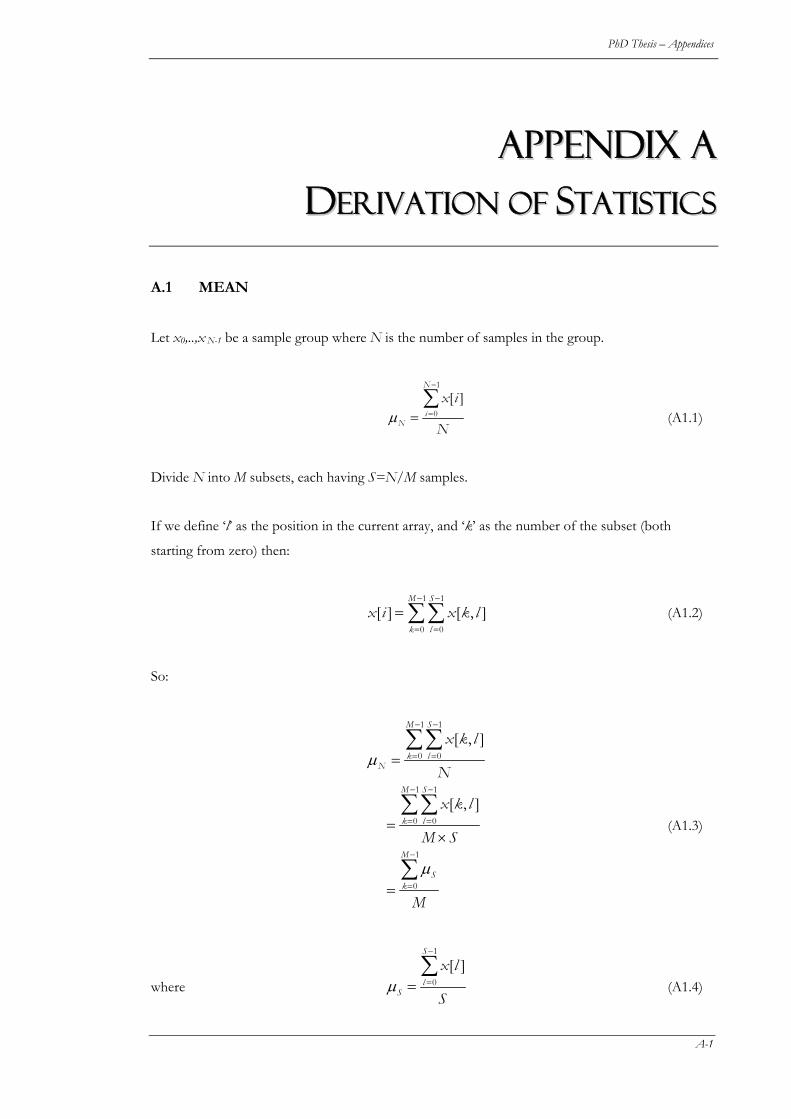
PhD Thesis – Appendices
AAPPPPEENNDDIIXX AA DDEERRIIVVAATTIIOONN OOFF SSTTAATTIISSTTIICCSS
A.1 MEAN
Let x0,..,x N-1 be a sample group where N is the number of samples in the group.
1
0
[ ]N
iN
x i
Nμ
−
==∑
(A1.1)
Divide N into M subsets, each having S=N/M samples.
If we define ‘l’ as the position in the current array, and ‘k’ as the number of the subset (both
starting from zero) then:
(A1.2) 1 1
0 0
[ ] [ , ]M S
k l
x i x k l− −
= =
= ∑∑
So:
1 1
0 0
1 1
0 0
1
0
[ , ]
[ , ]
M S
k lN
M S
k l
M
Sk
x k l
N
x k l
M S
M
μ
μ
− −
= =
− −
= =
−
=
=
=×
=
∑∑
∑∑
∑
(A1.3)
where
1
0
[ ]S
lS
x l
Sμ
−
==∑
(A1.4)
A-1

PhD Thesis – Appendices
A.2 VARIANCE
212
01
2 2
0
1 1 12 2
0 0 0
1 12 2
0 0
1 12
20 0
0
( [ ] )1
1 ( [ ] 2 [ ] )
1 [ ] 2 [ ]
1 [ ] 2 [ ]
[ ] [ ]2
[ ]
NN
iN
N Ni
N N N
N Ni i i
N N
N Ni i
N N
i iN N
SQk
x iN
x i x iN
x i x iN
x i x i NN
x i x i
N N
X k
μσ
μ μ
μ μ
μ μ
μ μ
−
=
−
=
− − −
= = =
− −
= =
− −
= =
=
−=
−
= ⋅ − +
⎧ ⎫= ⋅ − +⎨ ⎬⎩ ⎭⎧ ⎫= ⋅ − +⎨ ⎬⎩ ⎭
⎛ ⎞⎜ ⎟⎜ ⎟= − ⋅ +⎜ ⎟⎜ ⎟⎝ ⎠
=
∑
∑
∑ ∑ ∑
∑ ∑
∑ ∑
1 1
20
[ ]2
M M
Sk
N N
X k
M Mμ μ
− −
=
⎛ ⎞⎜ ⎟⎜ ⎟− ⋅ +⎜ ⎟⎜ ⎟⎝ ⎠
∑ ∑
(A1.5)
where
12
0
[ ][ ]
S
lSQ
x lX k
S
−
==∑
(A1.6)
and
1
1
[ ][ ]
S
lS
x lX k
S
−
==∑
(A1.7)
A-2
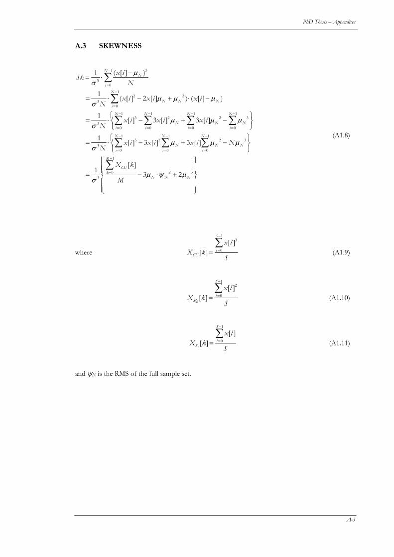
PhD Thesis – Appendices
A.3 SKEWNESS
31
30
12 2
30
1 1 1 13 2 2
30 0 0 0
1 1 13 2 2 3
30 0 0
3
( [ ] )1
1 ( [ ] 2 [ ] ) ( [ ] )
1 [ ] 3 [ ] 3 [ ]
1 [ ] 3 [ ] 3 [ ]
1
NN
iN
N N Ni
N N N N
N Ni i i i
N N N
N Ni i i
x iSkN
x i x i x iN
x i x i x iN
x i x i x i NN
X
μσ
μ μ μσ
μ μσ
μ μ μσ
σ
−
=
−
=
− − − −
= = = =
− − −
= = =
−= ⋅
= ⋅ − + ⋅ −
⎧ ⎫= ⋅ − + −⎨ ⎬
⎩ ⎭⎧ ⎫
= ⋅ − + −⎨ ⎬⎩ ⎭
=
∑
∑
∑ ∑ ∑ ∑
∑ ∑ ∑
3N
N
μ
1
2 30
[ ]3 2
M
CUk
N N N
k
Mμ ψ μ
−
=
⎧ ⎫⎪ ⎪⎪ ⎪− ⋅ +⎨ ⎬⎪ ⎪⎪ ⎪⎩ ⎭
∑
(A1.8)
where
13
0
[ ][ ]
S
lCU
x lX k
S
−
==∑
(A1.9)
12
0
[ ][ ]
S
lSQ
x lX k
S
−
==∑
(A1.10)
1
0
[ ][ ]
i
S
lS
x lX k
S
−
==∑
(A1.11)
and ψN is the RMS of the full sample set.
A-3
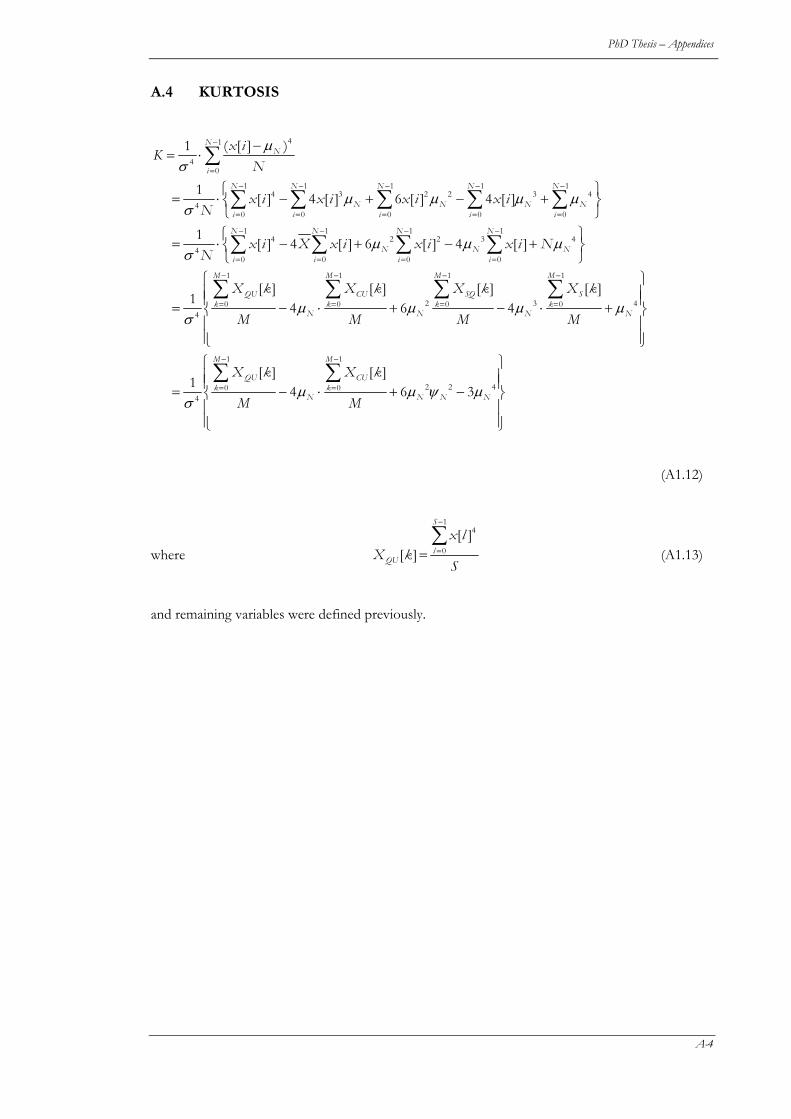
PhD Thesis – Appendices
A.4 KURTOSIS
41
40
1 1 1 1 14 3 2 2 3 4
40 0 0 0 0
1 1 1 14 2 2 3 4
40 0 0 0
1
04
( [ ] )1
1 [ ] 4 [ ] 6 [ ] 4 [ ]
1 [ ] 4 [ ] 6 [ ] 4 [ ]
[ ]1
NN
i
N N N N N
N N N Ni i i i i
N N N N
N N Ni i i i
M
QUk
x iKN
x i x i x i x iN
x i X x i x i x i NN
X k
μσ
μ μ μ μσ
μ μ μσ
σ
−
=
− − − − −
= = = = =
− − − −
= = = =
−
=
−= ⋅
⎧ ⎫= ⋅ − + − +⎨ ⎬
⎩ ⎭⎧ ⎫
= ⋅ − + − +⎨ ⎬⎩ ⎭
=
∑
∑ ∑ ∑ ∑ ∑
∑ ∑ ∑ ∑1 1 1
2 30 0 0
1 1
2 2 40 04
[ ] [ ] [ ]4 6 4
[ ] [ ]1 4 6 3
M M M
CU SQ Sk k k
N N N
M M
QU CUk k
N N N N
X k X k X k
M M M M
X k X k
M M
μ μ μ
μ μ ψ μσ
− − −
= = =
− −
= =
⎧ ⎫⎪ ⎪⎪ ⎪− ⋅ + − ⋅ +⎨ ⎬⎪ ⎪⎪ ⎪⎩ ⎭⎧ ⎫⎪ ⎪⎪ ⎪= − ⋅ + −⎨ ⎬⎪ ⎪⎪ ⎪⎩ ⎭
∑ ∑ ∑ ∑
∑ ∑
4Nμ
(A1.12)
where
14
0
[ ][ ]
S
lQU
x lX k
S
−
==∑
(A1.13)
and remaining variables were defined previously.
A-4
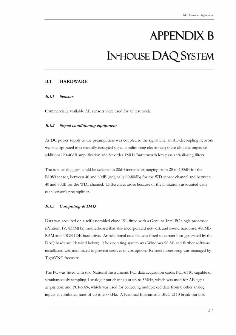
PhD Thesis – Appendices
AAPPPPEENNDDIIXX BB
IINN--HHOOUUSSEE DDAAQQ SSYYSSTTEEMM
B.1 HARDWARE
B.1.1 Sensors
Commercially available AE sensors were used for all test work.
B.1.2 Signal conditioning equipment
As DC power supply to the preamplifiers was coupled to the signal line, an AC-decoupling network
was incorporated into specially designed signal conditioning electronics; these also encompassed
additional 20-40dB amplification and 8th order 1MHz Butterworth low pass anti-aliasing filters.
The total analog gain could be selected in 20dB increments ranging from 20 to 100dB for the
B1080 sensor, between 40 and 60dB (originally 60-80dB) for the WD sensor channel and between
40 and 80dB for the WDI channel. Differences arose because of the limitations associated with
each sensor’s preamplifier.
B.1.3 Computing & DAQ
Data was acquired on a self-assembled clone PC, fitted with a Genuine Intel PC single processor
(Pentium IV, 833MHz) motherboard that also incorporated network and sound hardware, 480MB
RAM and 40GB IDE hard drive. An additional case fan was fitted to extract heat generated by the
DAQ hardware (detailed below). The operating system was Windows 98 SE and further software
installation was minimized to prevent sources of corruption. Remote monitoring was managed by
TightVNC freeware.
The PC was fitted with two National Instruments PCI data acquisition cards: PCI-6110, capable of
simultaneously sampling 4 analog input channels at up to 5MHz, which was used for AE signal
acquisition; and PCI-6024, which was used for collecting multiplexed data from 8 other analog
inputs at combined rates of up to 200 kHz. A National Instruments BNC-2110 break-out box
B-1

PhD Thesis – Appendices
facilitated the connection of conditioned pressure and temperature signals to this board. A
specially made cable was fabricated to connect the AE signal-conditioning unit to the PCI-6110
directly.
Both the PCI-6110 and PCI-6024 include a number of on-board analog amplifiers for additional
gain. These can be set from the National Instruments software program Measurements and
Automation Explorer (designed for configuration of NI hardware and generally referred to as ‘MAX’)
or programmatically from LabVIEW. MAX can also setup relationships between the incoming
analog signals and actual physical parameters for automatic scaling. This functionality was used for
all non-AE data channels, as it was not envisaged that gain would need to be altered during the
course of an experiment. The dynamic range of AE signals however, would most likely exceed the
optimum span of any one amplifier and consequently on-board gain selection was incorporated
into the main acquisition program. Additionally, pre-board gain was also included as a user control,
ensuring that all data was saved in terms of sensor units and therefore independent of the actual
amplifiers selected.
Once the system was configured and operating satisfactorily, an image was taken. This was then
reloaded prior to every new experiment to ensure stable and repeatable operation.
B.2 AE SOFTWARE
B.2.1 LabVIEW programs summary
Data acquisition and analysis programs were written predominantly in LabVIEW 6.02 (National
Instruments programming software) with a few key routines written (by others) in C++ to optimize
performance.
Subroutines for high-speed data-capture were based on the NIHSDL (high speed data logging)
API, which performed data streaming of the digitized data directly to disk, where it was stored in
compressed (16-12bit) little endian binary form. Functionality to facilitate software triggering and a
timeout was also included. A text header was written to the top of every file so that the sampling
and testing parameters could be viewed through a standard text editor.
B-2
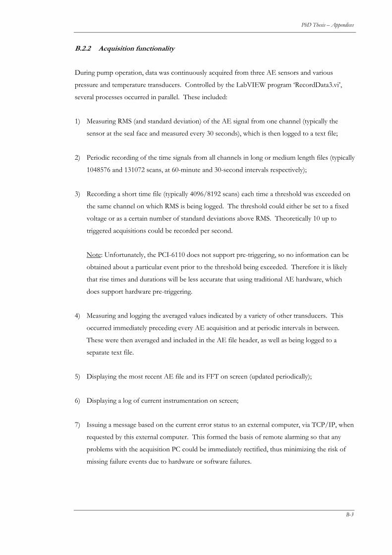
PhD Thesis – Appendices
B.2.2 Acquisition functionality
During pump operation, data was continuously acquired from three AE sensors and various
pressure and temperature transducers. Controlled by the LabVIEW program ‘RecordData3.vi’,
several processes occurred in parallel. These included:
1) Measuring RMS (and standard deviation) of the AE signal from one channel (typically the
sensor at the seal face and measured every 30 seconds), which is then logged to a text file;
2) Periodic recording of the time signals from all channels in long or medium length files (typically
1048576 and 131072 scans, at 60-minute and 30-second intervals respectively);
3) Recording a short time file (typically 4096/8192 scans) each time a threshold was exceeded on
the same channel on which RMS is being logged. The threshold could either be set to a fixed
voltage or as a certain number of standard deviations above RMS. Theoretically 10 up to
triggered acquisitions could be recorded per second.
Note: Unfortunately, the PCI-6110 does not support pre-triggering, so no information can be
obtained about a particular event prior to the threshold being exceeded. Therefore it is likely
that rise times and durations will be less accurate that using traditional AE hardware, which
does support hardware pre-triggering.
4) Measuring and logging the averaged values indicated by a variety of other transducers. This
occurred immediately preceding every AE acquisition and at periodic intervals in between.
These were then averaged and included in the AE file header, as well as being logged to a
separate text file.
5) Displaying the most recent AE file and its FFT on screen (updated periodically);
6) Displaying a log of current instrumentation on screen;
7) Issuing a message based on the current error status to an external computer, via TCP/IP, when
requested by this external computer. This formed the basis of remote alarming so that any
problems with the acquisition PC could be immediately rectified, thus minimizing the risk of
missing failure events due to hardware or software failures.
B-3
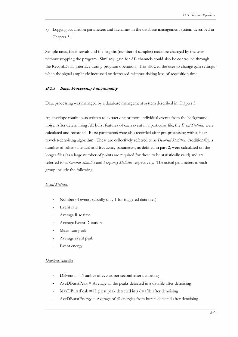
PhD Thesis – Appendices
8) Logging acquisition parameters and filenames in the database management system described in
Chapter 5.
Sample rates, file intervals and file lengths (number of samples) could be changed by the user
without stopping the program. Similarly, gain for AE channels could also be controlled through
the RecordData3 interface during program operation. This allowed the user to change gain settings
when the signal amplitude increased or decreased, without risking loss of acquisition time.
B.2.3 Basic Processing Functionality
Data processing was managed by a database management system described in Chapter 5.
An envelope routine was written to extract one or more individual events from the background
noise. After determining AE burst features of each event in a particular file, the Event Statistics were
calculated and recorded. Burst parameters were also recorded after pre-processing with a Haar
wavelet-denoising algorithm. These are collectively referred to as Denoised Statistics. Additionally, a
number of other statistical and frequency parameters, as defined in part 2, were calculated on the
longer files (as a large number of points are required for these to be statistically valid) and are
referred to as General Statistics and Frequency Statistics respectively. The actual parameters in each
group include the following:
Event Statistics
- Number of events (usually only 1 for triggered data files)
- Event rate
- Average Rise time
- Average Event Duration
- Maximum peak
- Average event peak
- Event energy
Denoised Statistics
- DEvents = Number of events per second after denoising
- AveDBurstPeak = Average all the peaks detected in a datafile after denoising
- MaxDBurstPeak = Highest peak detected in a datafile after denoising
- AveDBurstEnergy = Average of all energies from bursts detected after denoising
B-4
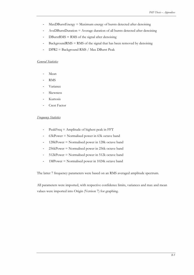
PhD Thesis – Appendices
- MaxDBurstEnergy = Maximum energy of bursts detected after denoising
- AveDBurstDuration = Average duration of all bursts detected after denoising
- DBurstRMS = RMS of the signal after denoising
- BackgroundRMS = RMS of the signal that has been removed by denoising
- DPR2 = Background RMS / Max DBurst Peak
General Statistics
- Mean
- RMS
- Variance
- Skewness
- Kurtosis
- Crest Factor
Frequency Statistics
- PeakFreq = Amplitude of highest peak in FFT
- 63kPower = Normalised power in 63k octave band
- 128kPower = Normalised power in 128k octave band
- 256kPower = Normalised power in 256k octave band
- 512kPower = Normalised power in 512k octave band
- 1MPower = Normalised power in 1024k octave band
The latter 7 frequency parameters were based on an RMS averaged amplitude spectrum.
All parameters were imported, with respective confidence limits, variances and max and mean
values were imported into Origin (Version 7) for graphing.
B-5
PhD Thesis – Appendices
C-1
AAPPPPEENNDDIIXX CC
SSIIGGNNAALL PPRROOCCEESSSSIINNGG AALLGGOORRIITTHHMMSS
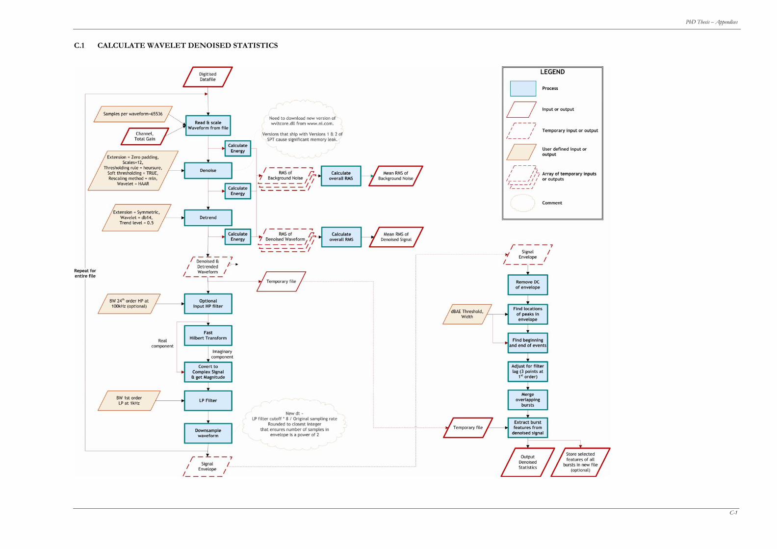
PhD Thesis – Appendices
C.1 CALCULATE WAVELET DENOISED STATISTICS
C-1

PhD Thesis – Appendices
C-2

PhD Thesis – Appendices
D-1
AAPPPPEENNDDIIXX DD
AAEEDDAATTAA TTAABBLLEESS
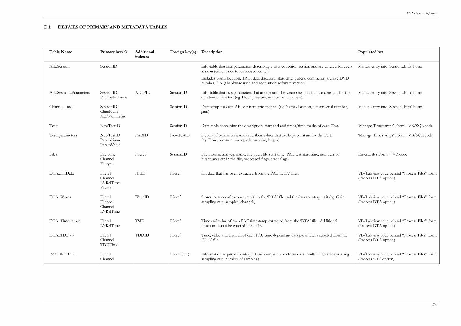
PhD Thesis – Appendices
D.1 DETAILS OF PRIMARY AND METADATA TABLES
Table Name Primary key(s) Additional indexes
Foreign key(s) Description Populated by:
AE_Session SessionID Info-table that lists parameters describing a data collection session and are entered for every session (either prior to, or subsequently).
Includes plant/location, TAG, data directory, start date, general comments, archive DVD number, DAQ hardware used and acquisition software version.
Manual entry into ‘Session_Info’ Form
AE_Session_Parameters SessionID, ParameterName
AETPID SessionID Info-table that lists parameters that are dynamic between sessions, but are constant for the duration of one test (eg. Flow, pressure, number of channels).
Manual entry into ‘Session_Info’ Form
Channel_Info SessionID ChanNum AE/Parametric
SessionID Data setup for each AE or parametric channel (eg. Name/location, sensor serial number, gain)
Manual entry into ‘Session_Info’ Form
Tests NewTestID SessionID Data-table containing the description, start and end times/time-marks of each Test. ‘Manage Timestamps’ Form +VB/SQL code
Test_parameters NewTestID ParamName ParamValue
PARID NewTestID Details of parameter names and their values that are kept constant for the Test. (eg. Flow, pressure, waveguide material, length)
‘Manage Timestamps’ Form +VB/SQL code
Files Filename Channel Filetype
Fileref SessionID File information (eg. name, filetypes, file start time, PAC test start time, numbers of hits/waves etc in the file, processed flags, error flags)
Enter_Files Form + VB code
DTA_HitData Fileref Channel LVRelTime Filepos
HitID Fileref Hit data that has been extracted from the PAC ‘DTA’ files. VB/Labview code behind “Process Files” form. (Process DTA option)
DTA_Waves Fileref Filepos Channel LVRelTime
WaveID Fileref Stores location of each wave within the ‘DTA’ file and the data to interpret it (eg. Gain, sampling rate, samples, channel.)
VB/Labview code behind “Process Files” form. (Process DTA option)
DTA_Timestamps Fileref LVRelTime
TSID Fileref Time and value of each PAC timestamp extracted from the ‘DTA’ file. Additional timestamps can be entered manually.
VB/Labview code behind “Process Files” form. (Process DTA option)
DTA_TDData Fileref Channel TDDTime
TDDID Fileref Time, value and channel of each PAC time dependant data parameter extracted from the ‘DTA’ file.
VB/Labview code behind “Process Files” form. (Process DTA option)
PAC_WF_Info Fileref Channel
Fileref (1:1) Information required to interpret and compare waveform data results and/or analysis. (eg. sampling rate, number of samples.)
VB/Labview code behind “Process Files” form. (Process WFS option)
D-1
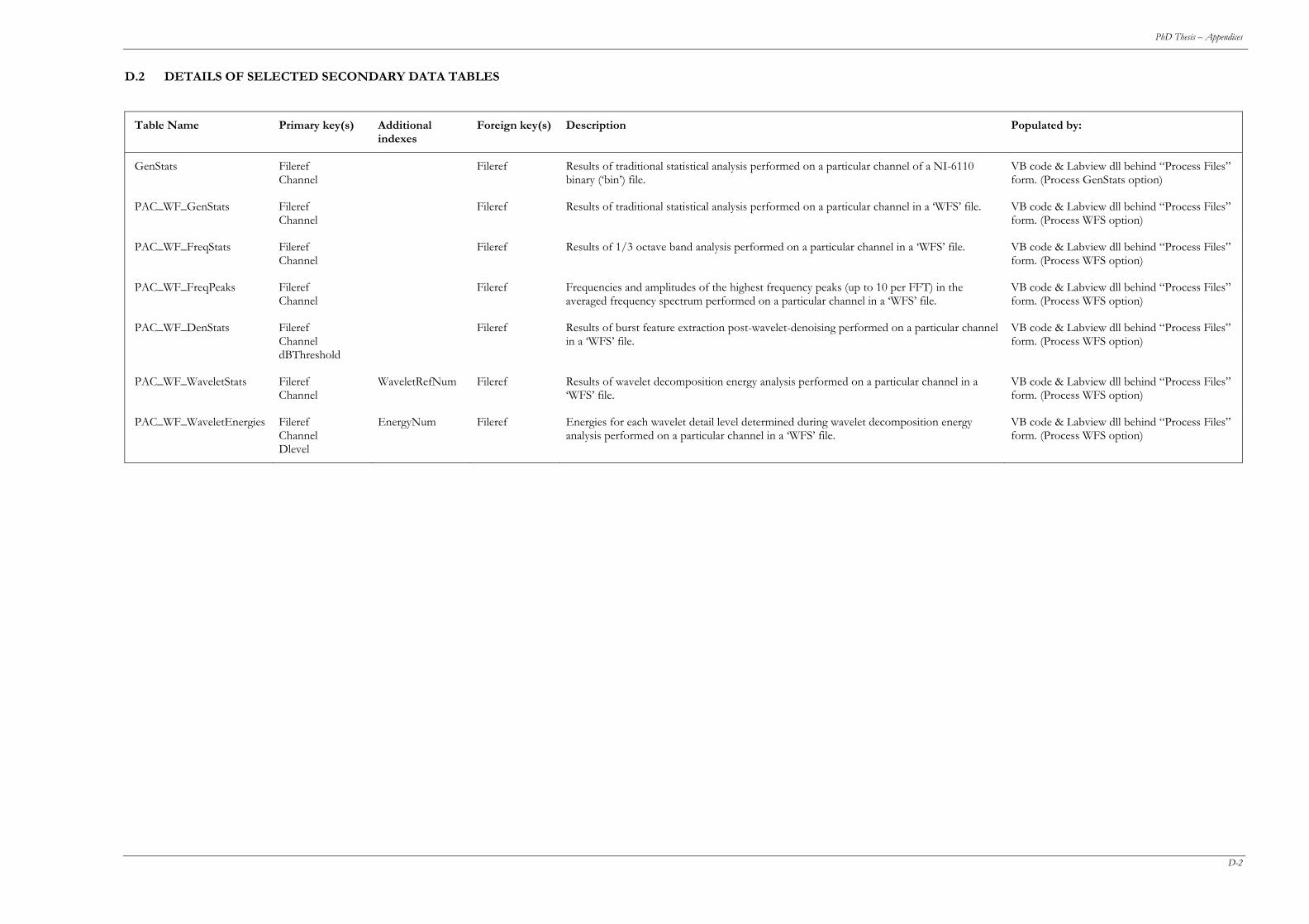
PhD Thesis – Appendices
D-2
D.2 DETAILS OF SELECTED SECONDARY DATA TABLES
Table Name Primary key(s) Additional indexes
Foreign key(s) Description Populated by:
GenStats Fileref Channel
Fileref Results of traditional statistical analysis performed on a particular channel of a NI-6110 binary (‘bin’) file.
VB code & Labview dll behind “Process Files” form. (Process GenStats option)
PAC_WF_GenStats Fileref Channel
Fileref Results of traditional statistical analysis performed on a particular channel in a ‘WFS’ file. VB code & Labview dll behind “Process Files” form. (Process WFS option)
PAC_WF_FreqStats Fileref Channel
Fileref Results of 1/3 octave band analysis performed on a particular channel in a ‘WFS’ file. VB code & Labview dll behind “Process Files” form. (Process WFS option)
PAC_WF_FreqPeaks Fileref Channel
Fileref Frequencies and amplitudes of the highest frequency peaks (up to 10 per FFT) in the averaged frequency spectrum performed on a particular channel in a ‘WFS’ file.
VB code & Labview dll behind “Process Files” form. (Process WFS option)
PAC_WF_DenStats Fileref Channel dBThreshold
Fileref Results of burst feature extraction post-wavelet-denoising performed on a particular channel in a ‘WFS’ file.
VB code & Labview dll behind “Process Files” form. (Process WFS option)
PAC_WF_WaveletStats Fileref Channel
WaveletRefNum Fileref Results of wavelet decomposition energy analysis performed on a particular channel in a ‘WFS’ file.
VB code & Labview dll behind “Process Files” form. (Process WFS option)
PAC_WF_WaveletEnergies Fileref Channel Dlevel
EnergyNum Fileref Energies for each wavelet detail level determined during wavelet decomposition energy analysis performed on a particular channel in a ‘WFS’ file.
VB code & Labview dll behind “Process Files” form. (Process WFS option)
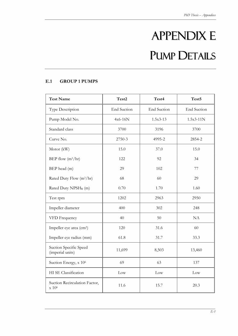
PhD Thesis – Appendices
AAPPPPEENNDDIIXX EE
PPUUMMPP DDEETTAAIILLSS
E.1 GROUP 1 PUMPS
Test Name Test2 Test4 Test5
Type Description End Suction End Suction End Suction
Pump Model No. 4x6-16N 1.5x3-13 1.5x3-11N
Standard class 3700 3196 3700
Curve No. 2750-3 4995-2 2854-2
Motor (kW) 15.0 37.0 15.0
BEP flow (m3/hr) 122 92 34
BEP head (m) 29 102 77
Rated Duty Flow (m3/hr) 68 60 29
Rated Duty NPSHR (m) 0.70 1.70 1.60
Test rpm 1202 2963 2950
Impeller diameter 400 302 248
VFD Frequency 40 50 NA
Impeller eye area (cm2) 120 31.6 60
Impeller eye radius (mm) 61.8 31.7 33.3
Suction Specific Speed (imperial units) 11,699 8,503 13,460
Suction Energy, x 106 69 63 137
HI SE Classification Low Low Low
Suction Recirculation Factor, x 106 11.6 15.7 20.3
E-1

PhD Thesis – Appendices
E.2 GROUP 2 PUMPS
Test Name Test6 Test7 Test8
Type Description End Suction End Suction End Suction
Pump Model No. 3x6-13 1x3-13B 1x3-13B
Standard class 3700 3700 3700
Curve No. 3893-2 2727-2 2727-2
Motor (kW) 55 30 30
BEP flow (m3/hr) 115/150 16.2/17.8 18/21
BEP head (m) 66 82/124 67/116
Rated Duty Flow (m3/hr) 121 20 20
Rated Duty NPSHR (m) 1.70 2** 2**
Test rpm 2236/2980 2263/2673 2267/2427
Impeller diameter 316 316 316
VFD Frequency 40/50 38/45 38/45
Impeller eye area (cm2) 126.5 45.2 45.2
Impeller eye radius (mm) 63.5 37.9 37.9
Suction Specific Speed (imperial units) 9,700 10,859 10,859
Suction Energy, x 106 108/145 73/87 73/79
HI SE Classification Low Low Low
Suction Recirculation Factor, x 106 14.1/18.8 16.0/18.9 16.0/17.2
E-2
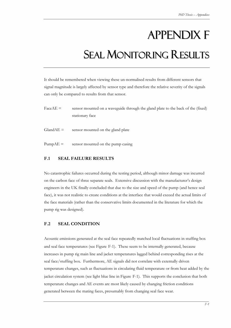
PhD Thesis – Appendices
AAPPPPEENNDDIIXX FF
SSEEAALL MMOONNIITTOORRIINNGG RREESSUULLTTSS
It should be remembered when viewing these un-normalised results from different sensors that
signal magnitude is largely affected by sensor type and therefore the relative severity of the signals
can only be compared to results from that sensor.
FaceAE = sensor mounted on a waveguide through the gland plate to the back of the (fixed)
stationary face
GlandAE = sensor mounted on the gland plate
PumpAE = sensor mounted on the pump casing
F.1 SEAL FAILURE RESULTS
No catastrophic failures occurred during the testing period, although minor damage was incurred
on the carbon face of three separate seals. Extensive discussion with the manufacturer’s design
engineers in the UK finally concluded that due to the size and speed of the pump (and hence seal
face), it was not realistic to create conditions at the interface that would exceed the actual limits of
the face materials (rather than the conservative limits documented in the literature for which the
pump rig was designed).
F.2 SEAL CONDITION
Acoustic emissions generated at the seal face repeatedly matched local fluctuations in stuffing box
and seal face temperatures (see Figure F-1). These seem to be internally generated, because
increases in pump rig main line and jacket temperatures lagged behind corresponding rises at the
seal face/stuffing box. Furthermore, AE signals did not correlate with externally driven
temperature changes, such as fluctuations in circulating fluid temperature or from heat added by the
jacket circulation system (see light blue line in Figure F-1). This supports the conclusion that both
temperature changes and AE events are most likely caused by changing friction conditions
generated between the mating faces, presumably from changing seal face wear.
F-1
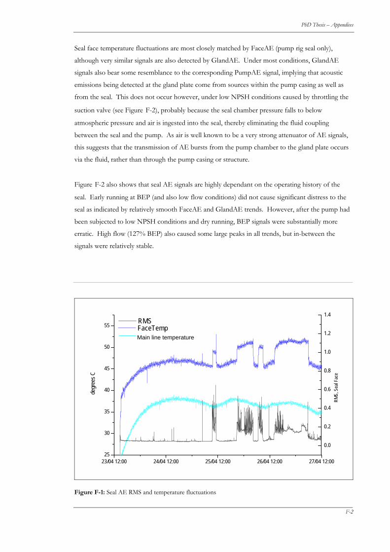
PhD Thesis – Appendices
Seal face temperature fluctuations are most closely matched by FaceAE (pump rig seal only),
although very similar signals are also detected by GlandAE. Under most conditions, GlandAE
signals also bear some resemblance to the corresponding PumpAE signal, implying that acoustic
emissions being detected at the gland plate come from sources within the pump casing as well as
from the seal. This does not occur however, under low NPSH conditions caused by throttling the
suction valve (see Figure F-2), probably because the seal chamber pressure falls to below
atmospheric pressure and air is ingested into the seal, thereby eliminating the fluid coupling
between the seal and the pump. As air is well known to be a very strong attenuator of AE signals,
this suggests that the transmission of AE bursts from the pump chamber to the gland plate occurs
via the fluid, rather than through the pump casing or structure.
Figure F-2 also shows that seal AE signals are highly dependant on the operating history of the
seal. Early running at BEP (and also low flow conditions) did not cause significant distress to the
seal as indicated by relatively smooth FaceAE and GlandAE trends. However, after the pump had
been subjected to low NPSH conditions and dry running, BEP signals were substantially more
erratic. High flow (127% BEP) also caused some large peaks in all trends, but in-between the
signals were relatively stable.
23/04 12:00 24/04 12:00 25/04 12:00 26/04 12:00 27/04 12:0025
30
35
40
45
50
55
0.0
0.2
0.4
0.6
0.8
1.0
1.2
1.4
FaceTemp
degr
ees C
RMS
RMS
, Sea
l Fac
e
Main line temperature
Figure F-1: Seal AE RMS and temperature fluctuations
F-2
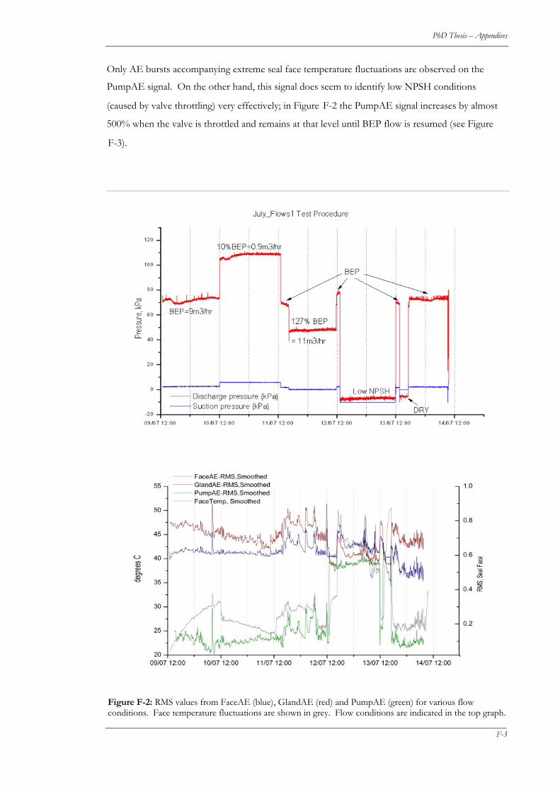
PhD Thesis – Appendices
Only AE bursts accompanying extreme seal face temperature fluctuations are observed on the
PumpAE signal. On the other hand, this signal does seem to identify low NPSH conditions
(caused by valve throttling) very effectively; in Figure F-2 the PumpAE signal increases by almost
500% when the valve is throttled and remains at that level until BEP flow is resumed (see Figure
F-3).
Figure F-2: RMS values from FaceAE (blue), GlandAE (red) and PumpAE (green) for various flow conditions. Face temperature fluctuations are shown in grey. Flow conditions are indicated in the top graph.
F-3
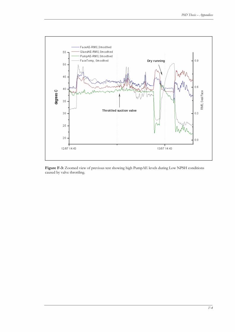
PhD Thesis – Appendices
Throttled suction valve
Dry running
Figure F-3: Zoomed view of previous test showing high PumpAE levels during Low NPSH conditions caused by valve throttling.
F-4

PhD Thesis – Appendices
F-5


