The Application of Model Predictive Control (MPC) to Fast Systems such as Autonomous Ground Vehicles (AGV

IOSR Journal of Computer Engineering (IOSR-JCE)

e-ISSN: 2278-0661, p- ISSN: 2278-8727Volume 16, Issue 3, Ver. IV (May-Jun. 2014), PP 27-37

www.iosrjournals.org

www.iosrjournals.org 27 | Page

The Application of Model Predictive Control (MPC) to Fast

Systems such as Autonomous Ground Vehicles (AGV)

Solomon Sunday Oyelere Department of Computer Science Modibbo Adama University of Technology Yola.

[email protected]

Abstract: This paper investigates the application of Model Predictive Control (MPC) to fast systems such as

Autonomous Ground Vehicles (AGV) or mobile robots. The control of Autonomous ground vehicles (AGV) is

challenging because of nonholonomic constraints, uncertainties, speed, accuracy of controls and the vehicle's

terrain of operation. Two nonlinear models: a car-like model and a bicycle model are considered. A Nonlinear

MPC (NMPC) was developed. A trajectory tracking performance index for both models was studied. After

thorough and extensive simulation, it is observed that both models are applicable in the context of NMPC and

the constraints on model variables were adequately respected. The trajectories were successfully tracked and

thus clearly indicate the efficiency and effectiveness of the MPC technique. In order to improve on speed and

reduce the computational effort required for the optimization problem, a Linear MPC (LMPC) was implemented

with both models. This is possible by successive linearization along the reference trajectory and formulating a

quadratic optimization problem which is solved by implementing an interior-point quadratic programming

algorithm. For both AGV models, analysis concerning the reduced computational efforts is presented in order to

show the viability of LMPC technique developed.

Keywords: Model predictive control, Autonomous Ground Vehicle, Optimization, Interior-point Quadratic

Programming.

I. Introduction The universe is facing an ever rapid increasing interest in the development and application of

Autonomous Ground Vehicles (AGV). The areas of AGVs application are enormous and innovation in this

direction is continuously revolving. In a general sense, an Autonomous Ground Vehicle is mechanical

equipment that operates across the surface of the ground without any onboard human presence. Autonomous

Ground Vehicles and their applications in scientific and planetary exploration, health technology, security,

nuclear power industry, transportation and logistics, military operation like mine deactivation, surveillance,

education, excavation, entertainment, agriculture (farm vehicles), housekeeping, mining and exploration,

inspection and maintenance, completion of complex, dangerous and remote environment tasks, reduction of

vehicle accident on highways, etc. These applications often involve limitations on communications that require

AGVs to navigate autonomously for extended distances and extended periods of time. Under these

circumstances, AGVs must be equipped with facilities like cameras and sensors for navigation and detection of

obstacles in their path. The operational challenges of AGVs heavily depend on the terrain of operation of the

vehicle. Accordingly, an AGV should manage to contain a range of uncertainties and external influences; should

be able to perform reliable sensing and perceptions, adjust itself to terrain properties and external events (static

or dynamic obstacles), move autonomously and intelligently to accomplish the intended tasks optimally, etc. To

realize these, real-time and fast control strategies are of significant importance. Model Predictive Control (MPC)

has gained tremendous attention in recent years for trajectory planning and tracking of AGV. Since AGVs are

generally equipped with sensors that provide information about their current location, MPC provides a good

framework for this problem. Considering the fact that the vehicles location should have to be continuously

updated on-line in real-time, in order to follow a planned trajectory and avoid obstacles, Model Predictive

Control can be considered appropriate in this scenario [1], [2].

Model Predictive Control performs an online optimization of the output of an optimal control problem

over a finite horizon [3], [4]. The basic idea of MPC is the use of a model to predict the output of a process over

a future time horizon by obtaining a control sequence which minimizes an objective function [5].

An analogy can be made between the MPC and the act of driving a car in [6]. The driver knows the desired

reference trajectory for a finite horizon: his field of view of the road. Taking into account the characteristics of

the car (a mental model of the car and speed limits, acceleration and maneuverability) and possible roadblocks

(like holes, intersections and other cars), he will decide what action to take (increase or decrease speed, turning

direction to one side or the other) so that the desired trajectory is traversed. This control action is then applied

for a short time and the procedure is repeated for the next control action now with the field of view updated. It is

The Application of Model Predictive Control (MPC) to Fast Systems such as Autonomous Ground


observed that, using the model of the car, predictions of behavior is used, based on what the driver is seeing

ahead.

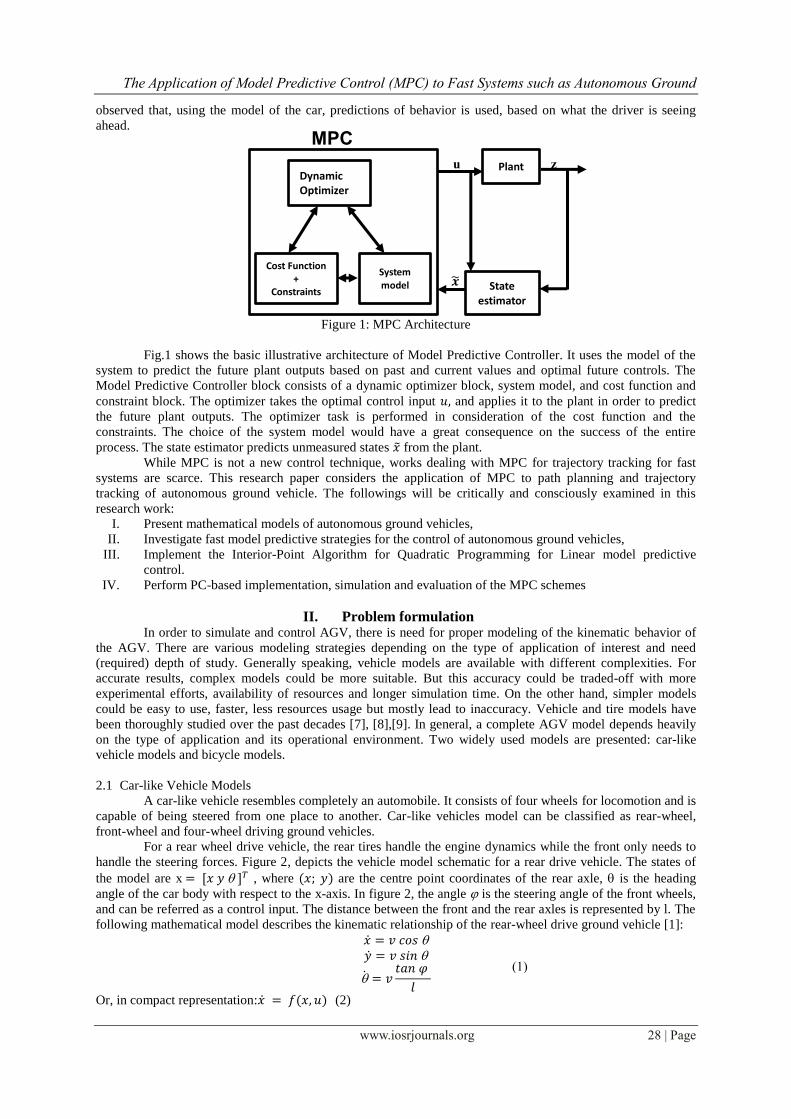
Figure 1: MPC Architecture

Fig.1 shows the basic illustrative architecture of Model Predictive Controller. It uses the model of the

system to predict the future plant outputs based on past and current values and optimal future controls. The

Model Predictive Controller block consists of a dynamic optimizer block, system model, and cost function and

constraint block. The optimizer takes the optimal control input and applies it to the plant in order to predict

the future plant outputs. The optimizer task is performed in consideration of the cost function and the

constraints. The choice of the system model would have a great consequence on the success of the entire

process. The state estimator predicts unmeasured states from the plant.

While MPC is not a new control technique, works dealing with MPC for trajectory tracking for fast

systems are scarce. This research paper considers the application of MPC to path planning and trajectory

tracking of autonomous ground vehicle. The followings will be critically and consciously examined in this

research work:

I. Present mathematical models of autonomous ground vehicles,

II. Investigate fast model predictive strategies for the control of autonomous ground vehicles,

III. Implement the Interior-Point Algorithm for Quadratic Programming for Linear model predictive

control.

IV. Perform PC-based implementation, simulation and evaluation of the MPC schemes

II. Problem formulation In order to simulate and control AGV, there is need for proper modeling of the kinematic behavior of

the AGV. There are various modeling strategies depending on the type of application of interest and need

(required) depth of study. Generally speaking, vehicle models are available with different complexities. For

accurate results, complex models could be more suitable. But this accuracy could be traded-off with more

experimental efforts, availability of resources and longer simulation time. On the other hand, simpler models

could be easy to use, faster, less resources usage but mostly lead to inaccuracy. Vehicle and tire models have

been thoroughly studied over the past decades [7], [8],[9]. In general, a complete AGV model depends heavily

on the type of application and its operational environment. Two widely used models are presented: car-like

vehicle models and bicycle models.

2.1 Car-like Vehicle Models

A car-like vehicle resembles completely an automobile. It consists of four wheels for locomotion and is

capable of being steered from one place to another. Car-like vehicles model can be classified as rear-wheel,

front-wheel and four-wheel driving ground vehicles.

For a rear wheel drive vehicle, the rear tires handle the engine dynamics while the front only needs to

handle the steering forces. Figure 2, depicts the vehicle model schematic for a rear drive vehicle. The states of

the model are x , where are the centre point coordinates of the rear axle, is the heading

angle of the car body with respect to the x-axis. In figure 2, the angle is the steering angle of the front wheels,

and can be referred as a control input. The distance between the front and the rear axles is represented by l. The

following mathematical model describes the kinematic relationship of the rear-wheel drive ground vehicle [1]:

Or, in compact representation: (2)

𝒙

z u

MPC Cont

Dynamic Optimizer

Cost Function +

Constraints

System model

Plant

State estimator

(1)



The steering angle and line velocity are used as a control input, i.e. .

2.2 Bicycle Model

A bicycle model can be used to represent a four wheel vehicle; any vehicle model can be described as a

bicycle model [10]. In a bicycle model, the two front wheels are lumped into one wheel and the two back wheels

are also lumped into one. For the bicycle model, the complete form of the dynamic model of the vehicle is given

by [11]:

[

]

[

]

[

]

[

]

(3)

the state vector is represented as , = Vehicle side slip angle,

= Vehicle yaw angle,

= Vehicle yaw rate,

= x-coordinate of the vehicle's centre of gravity in inertial frame,

= y-coordinate of the vehicle's centre of gravity in inertial frame.While the control vector is represented by

, where is the front tyre steering angle.

Applying Euler's approximation to equations 1, the discrete-time model for the AGV motion is given

below:

(4)

Where,

,T is the sampling period and k a sampling instant. Represented in a compact form as,

(5)

III. Nonlinear Model Predictive Control (NMPC) NMPC is a class of MPC theories that are based on the use of nonlinear system models:

in the prediction. The cost function can be non-quadratic, and the optimization problem

consists of nonlinear constraints on states and controls. Therefore, the optimization problem to be solved at each

sampling instant is nonlinear leading to nonlinear model predictive control. Generally, linear MPC could handle

problems with multivariable and constraints efficiently but in some special situations, nonlinear process

behaviors and the choice of admissible operating region could hamper the performance and stability of the

system process. Therefore, sometimes it is pertinent to choose NMPC.

3.1 Formulation of Performance Index

Consider an AGV nonlinear model of the following form; ( ) where is the state

vector, represent the control inputs and t is the time. In discrete time, the above model can be represented by a

difference equation of the following form:

(6) where is the sampling instant, { } Typical performance index to be minimized is formulated

as follows:

∑

∑ (7)

where is prediction horizon and is control horizon, and are weighting matrices

which are used to penalize the state error and control error,respectively, with and . The following

constraint expression can beapplicable depending on individual cases:

where is the set of possible values for the system states and is the set of possiblecontrol inputs.



Thus, the optimization problem to be solved at each sampling instant can be put to find a control sequence

and a sequence of states such that minimize the cost function and comply with the constraints as

formulated below:

m

subject to: (8)

Where and are the states and control vector respectively. The initial condition of the state is , and

is a general system of differential algebraic equations (DAEs). The optimal performance index to be obtained

is while the optimal control sequence is as follows:

the optimal states sequence is as follows:

During the next sampling instant , the entire procedure is repeated while the statesare updated

and the time window is shifted forward.

3.2 Trajectory Tracking with NMPC

The problem of trajectory tracking by autonomous ground vehicle (AGV) involves making the AGV

follow a preplanned trajectory at varying time.

For a trajectory tracking problem, we need to compute a control law such that:

(9)

where

xref [

]

Is the reference trajectory. Normally, a virtual reference AGV with the same kinematic model could be

associated with the actual AGV. The virtual AGV provide the reference trajectory which would be tracked.

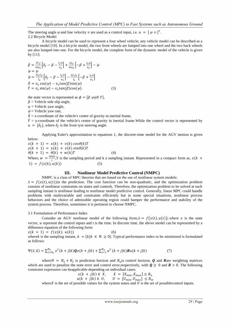
Figure 2 is a block diagram of the trajectory tracking system.

Figure 2: Block diagram of trajectory tracking system

In Fig. 2, is the AGV's reference point, is the reference AGV's trajectory, represents the error

with respect to the reference AGV, is the Autonomous GroundVehicle’s trajectory, represent the optimal

control obtained after MPC and is the optimal control applied on the actual AGV. The reference trajectory of

the virtual AGV is given below:

(10)

For a NMPC trajectory tracking we define the following relationships:

(11)

the following performance index to be minimized is formulated as follows:

∑ (12)

-

MPC

𝒖𝒓

𝒖

𝒖

𝒙⬚

𝒙 x

𝒙𝒓𝒆𝒇

Reference

AGV

Autonomous Ground Vehicle



where N is the prediction horizon, and are the weighing matrices. Weconsider that there is a

constraint bound on the control variables:

where represent the lower bound and represent the upper bound. Similarly, constraint on the states can

be generally expressed as .

Therefore, at each sampling instant k, for a NMPC trajectory tracking, the following problem is solved:

m

subject to: (13)

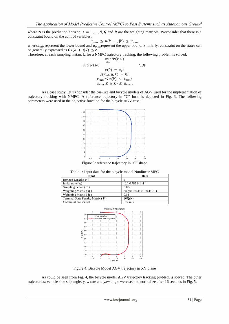
As a case study, let us consider the car-like and bicycle models of AGV used for the implementation of

trajectory tracking with NMPC. A reference trajectory in "C" form is depicted in Fig. 3. The following

parameters were used in the objective function for the bicycle AGV case;

Figure 3: reference trajectory in “C” shape

Table 1: Input data for the bicycle model Nonlinear MPC Input Data

Horizon Length ( N ) 5

Initial state (x0) [0.1 0.785 0 1 -1]T

Sampling period ( T ) 0:05s

Weighting Matrix ( Q ) diag(0.1; 0.1; 0.1; 0.1; 0.1)

Weighting Matrix ( R ) 0.01

Terminal State Penalty Matrix ( P ) 20Q(N)

Constraint on Control 0:35m/s

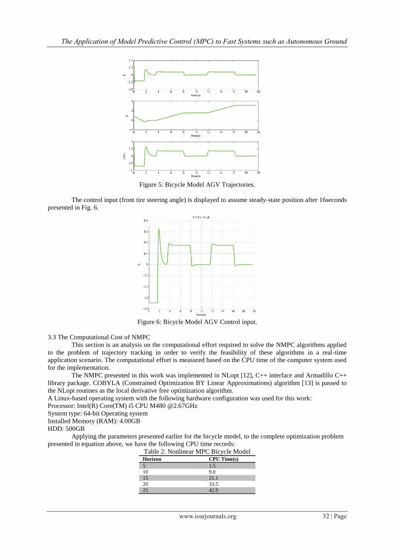
Figure 4: Bicycle Model AGV trajectory in XY plane

As could be seen from Fig. 4, the bicycle model AGV trajectory tracking problem is solved. The other

trajectories; vehicle side slip angle, yaw rate and yaw angle were seen to normalize after 16 seconds in Fig. 5.



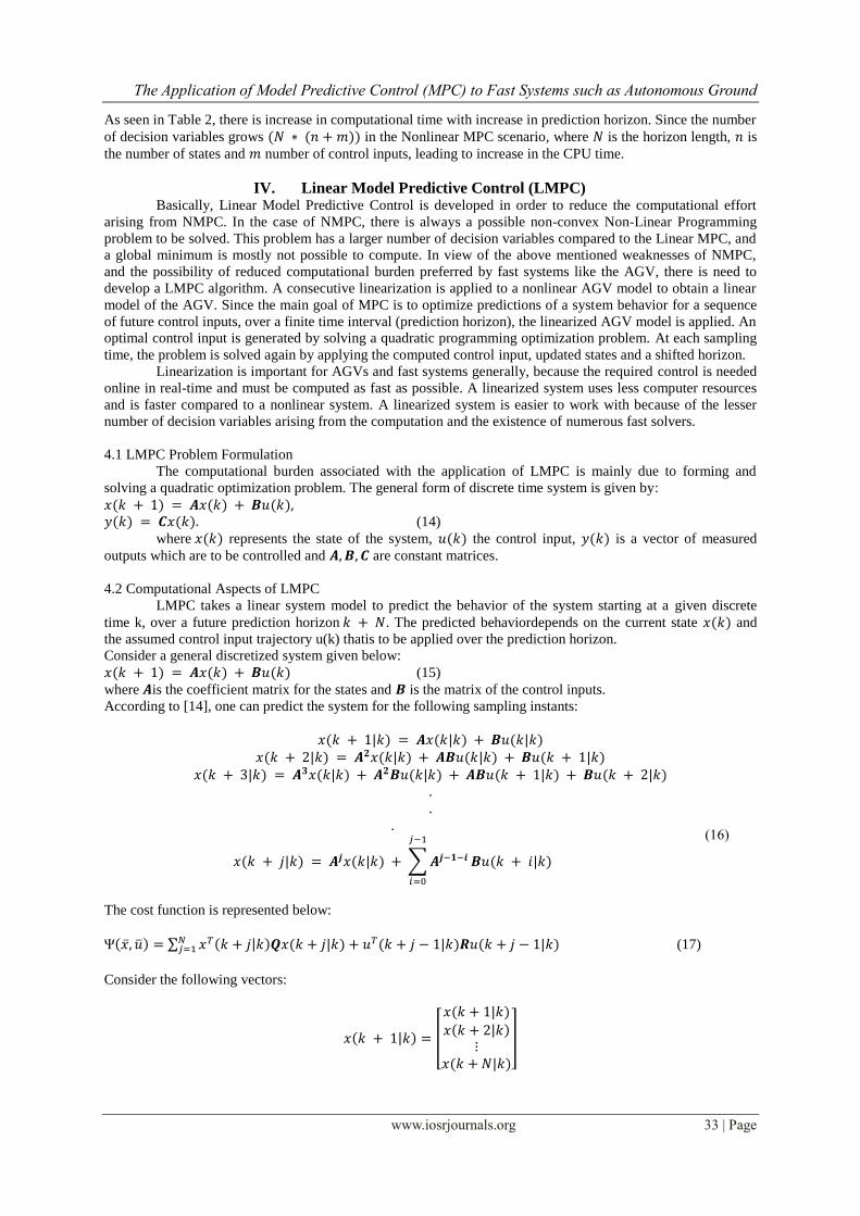
Figure 5: Bicycle Model AGV Trajectories.

The control input (front tire steering angle) is displayed to assume steady-state position after 16seconds

presented in Fig. 6.

Figure 6: Bicycle Model AGV Control input.

3.3 The Computational Cost of NMPC

This section is an analysis on the computational effort required to solve the NMPC algorithms applied

to the problem of trajectory tracking in order to verify the feasibility of these algorithms in a real-time

application scenario. The computational effort is measured based on the CPU time of the computer system used

for the implementation.

The NMPC presented in this work was implemented in NLopt [12], C++ interface and Armadillo C++

library package. COBYLA (Constrained Optimization BY Linear Approximations) algorithm [13] is passed to

the NLopt routines as the local derivative free optimization algorithm.

A Linux-based operating system with the following hardware configuration was used for this work:

Processor: Intel(R) Core(TM) i5 CPU M480 @2.67GHz

System type: 64-bit Operating system

Installed Memory (RAM): 4.00GB

HDD: 500GB

Applying the parameters presented earlier for the bicycle model, to the complete optimization problem

presented in equation above, we have the following CPU time records:

Table 2: Nonlinear MPC Bicycle Model Horizon CPU Time(s)

5 1.5

10 9.0

15 21.1 20 33.5

25 42.9



As seen in Table 2, there is increase in computational time with increase in prediction horizon. Since the number

of decision variables grows in the Nonlinear MPC scenario, where is the horizon length, is

the number of states and number of control inputs, leading to increase in the CPU time.

IV. Linear Model Predictive Control (LMPC) Basically, Linear Model Predictive Control is developed in order to reduce the computational effort

arising from NMPC. In the case of NMPC, there is always a possible non-convex Non-Linear Programming

problem to be solved. This problem has a larger number of decision variables compared to the Linear MPC, and

a global minimum is mostly not possible to compute. In view of the above mentioned weaknesses of NMPC,

and the possibility of reduced computational burden preferred by fast systems like the AGV, there is need to

develop a LMPC algorithm. A consecutive linearization is applied to a nonlinear AGV model to obtain a linear

model of the AGV. Since the main goal of MPC is to optimize predictions of a system behavior for a sequence

of future control inputs, over a finite time interval (prediction horizon), the linearized AGV model is applied. An

optimal control input is generated by solving a quadratic programming optimization problem. At each sampling

time, the problem is solved again by applying the computed control input, updated states and a shifted horizon.

Linearization is important for AGVs and fast systems generally, because the required control is needed

online in real-time and must be computed as fast as possible. A linearized system uses less computer resources

and is faster compared to a nonlinear system. A linearized system is easier to work with because of the lesser

number of decision variables arising from the computation and the existence of numerous fast solvers.

4.1 LMPC Problem Formulation

The computational burden associated with the application of LMPC is mainly due to forming and

solving a quadratic optimization problem. The general form of discrete time system is given by:

(14)

where represents the state of the system, the control input, is a vector of measured

outputs which are to be controlled and are constant matrices.

4.2 Computational Aspects of LMPC

LMPC takes a linear system model to predict the behavior of the system starting at a given discrete

time k, over a future prediction horizon . The predicted behaviordepends on the current state and

the assumed control input trajectory u(k) thatis to be applied over the prediction horizon.

Consider a general discretized system given below:

(15) where is the coefficient matrix for the states and is the matrix of the control inputs.

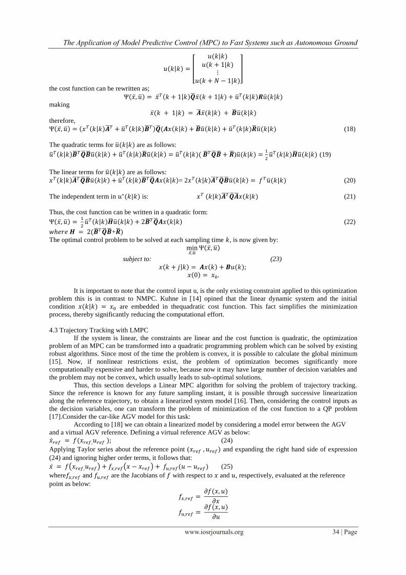
According to [14], one can predict the system for the following sampling instants:

∑

The cost function is represented below:

∑ (17)

Consider the following vectors:

[

⋮

]

(16)



[

⋮

]

the cost function can be rewritten as;

making

therefore,

(18)

The quadratic terms for are as follows:

)

(19)

The linear terms for are as follows:

= 2 (20)

The independent term in is: (21)

Thus, the cost function can be written in a quadratic form:

(22)

+

The optimal control problem to be solved at each sampling time , is now given by:

m

subject to: (23)

It is important to note that the control input u, is the only existing constraint applied to this optimization

problem this is in contrast to NMPC. Kuhne in [14] opined that the linear dynamic system and the initial

condition are embedded in thequadratic cost function. This fact simplifies the minimization

process, thereby significantly reducing the computational effort.

4.3 Trajectory Tracking with LMPC

If the system is linear, the constraints are linear and the cost function is quadratic, the optimization

problem of an MPC can be transformed into a quadratic programming problem which can be solved by existing

robust algorithms. Since most of the time the problem is convex, it is possible to calculate the global minimum

[15]. Now, if nonlinear restrictions exist, the problem of optimization becomes significantly more

computationally expensive and harder to solve, because now it may have large number of decision variables and

the problem may not be convex, which usually leads to sub-optimal solutions.

Thus, this section develops a Linear MPC algorithm for solving the problem of trajectory tracking.

Since the reference is known for any future sampling instant, it is possible through successive linearization

along the reference trajectory, to obtain a linearized system model [16]. Then, considering the control inputs as

the decision variables, one can transform the problem of minimization of the cost function to a QP problem

[17].Consider the car-like AGV model for this task:

According to [18] we can obtain a linearized model by considering a model error between the AGV

and a virtual AGV reference. Defining a virtual reference AGV as below: (24)

Applying Taylor series about the reference point ( and expanding the right hand side of expression

(24) and ignoring higher order terms, it follows that:

( ) ( ) (25)

where and are the Jacobians of with respect to and , respectively, evaluated at the reference

point as below:

𝜕

𝜕

𝜕

𝜕



Therefore, substituting the expression 25 in 1, and setting A = and ; it follows that:

where

In order to obtain a linearized model in discrete time, we employ the Euler method to discretize

equation 1, the result is given below:

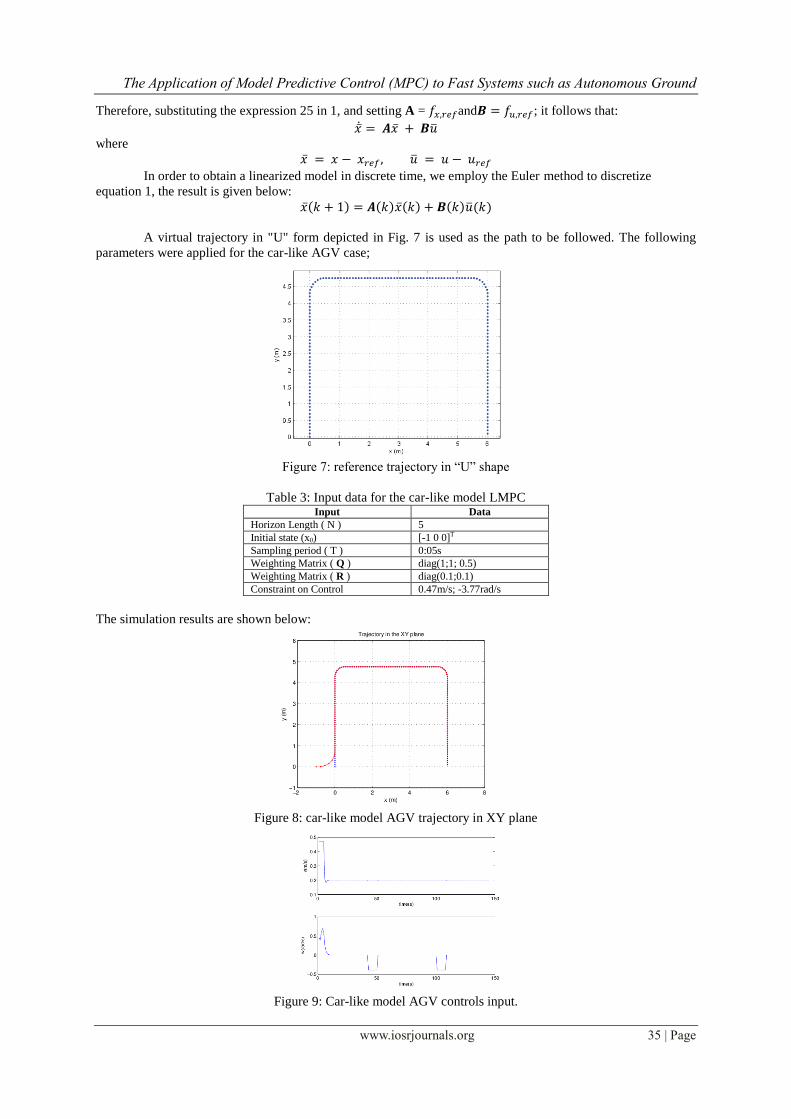
A virtual trajectory in "U" form depicted in Fig. 7 is used as the path to be followed. The following

parameters were applied for the car-like AGV case;

Figure 7: reference trajectory in “U” shape

Table 3: Input data for the car-like model LMPC Input Data

Horizon Length ( N ) 5

Initial state (x0) [-1 0 0]T

Sampling period ( T ) 0:05s

Weighting Matrix ( Q ) diag(1;1; 0.5)

Weighting Matrix ( R ) diag(0.1;0.1)

Constraint on Control 0.47m/s; -3.77rad/s

The simulation results are shown below:

Figure 8: car-like model AGV trajectory in XY plane

Figure 9: Car-like model AGV controls input.



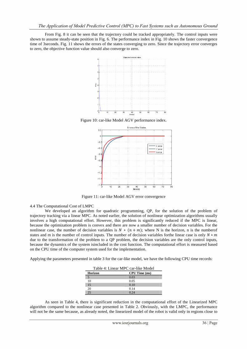
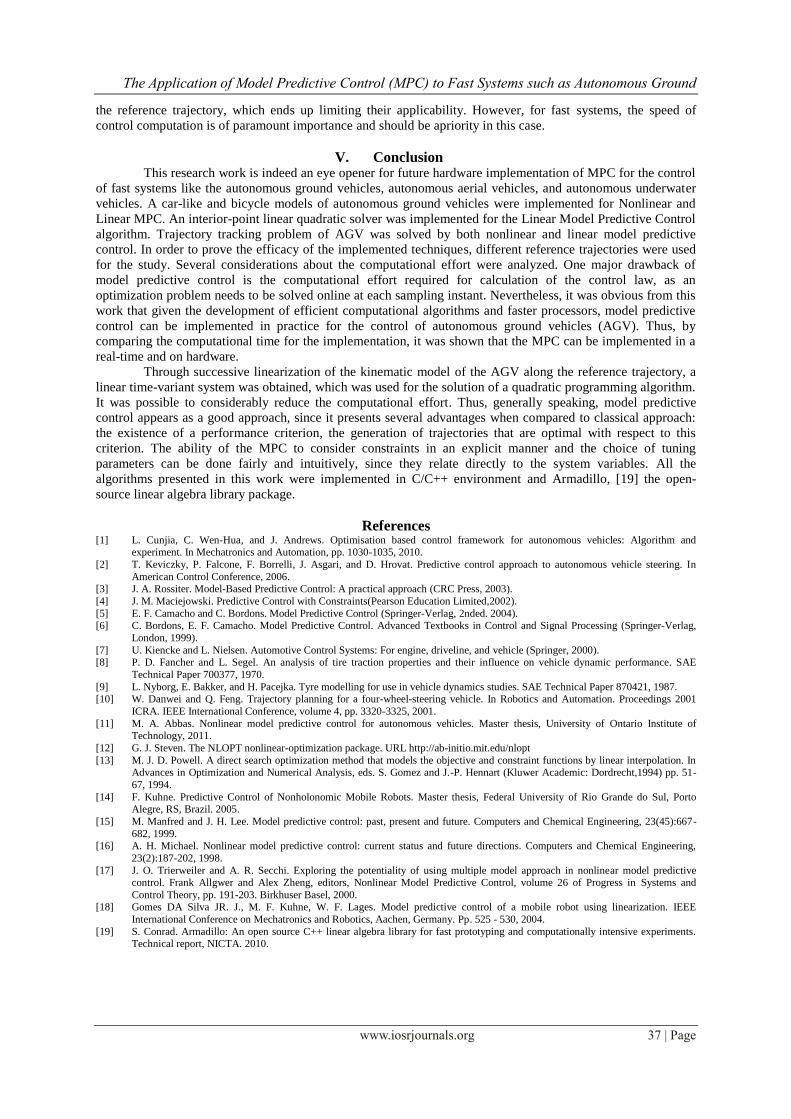
From Fig. 8 it can be seen that the trajectory could be tracked appropriately. The control inputs were

shown to assume steady-state position in Fig. 6. The performance index in Fig. 10 shows the faster convergence

time of 3seconds. Fig. 11 shows the errors of the states converging to zero. Since the trajectory error converges

to zero, the objective function value should also converge to zero.

Figure 10: car-like Model AGV performance index.

Figure 11: car-like Model AGV error convergence

4.4 The Computational Cost of LMPC

We developed an algorithm for quadratic programming, QP, for the solution of the problem of

trajectory tracking via a linear MPC. As noted earlier, the solution of nonlinear optimization algorithms usually

involves a high computational effort. However, this problem is significantly reduced if the MPC is linear,

because the optimization problem is convex and there are now a smaller number of decision variables. For the

nonlinear case, the number of decision variables is where N is the horizon, n is the numberof

states and m is the number of control inputs. The number of decision variables forthe linear case is only

due to the transformation of the problem to a QP problem, the decision variables are the only control inputs,

because the dynamics of the system isincluded in the cost function. The computational effort is measured based

on the CPU time of the computer system used for the implementation.

Applying the parameters presented in table 3 for the car-like model, we have the following CPU time records:

Table 4: Linear MPC car-like Model Horizon CPU Time (ms)

5 0.03 10 0.05

15 0.10

20 0.14 25 0.24

As seen in Table 4, there is significant reduction in the computational effort of the Linearized MPC

algorithm compared to the nonlinear case presented in Table 2. Obviously, with the LMPC, the performance

will not be the same because, as already noted, the linearized model of the robot is valid only in regions close to



the reference trajectory, which ends up limiting their applicability. However, for fast systems, the speed of

control computation is of paramount importance and should be apriority in this case.

V. Conclusion This research work is indeed an eye opener for future hardware implementation of MPC for the control

of fast systems like the autonomous ground vehicles, autonomous aerial vehicles, and autonomous underwater

vehicles. A car-like and bicycle models of autonomous ground vehicles were implemented for Nonlinear and

Linear MPC. An interior-point linear quadratic solver was implemented for the Linear Model Predictive Control

algorithm. Trajectory tracking problem of AGV was solved by both nonlinear and linear model predictive

control. In order to prove the efficacy of the implemented techniques, different reference trajectories were used

for the study. Several considerations about the computational effort were analyzed. One major drawback of

model predictive control is the computational effort required for calculation of the control law, as an

optimization problem needs to be solved online at each sampling instant. Nevertheless, it was obvious from this

work that given the development of efficient computational algorithms and faster processors, model predictive

control can be implemented in practice for the control of autonomous ground vehicles (AGV). Thus, by

comparing the computational time for the implementation, it was shown that the MPC can be implemented in a

real-time and on hardware.

Through successive linearization of the kinematic model of the AGV along the reference trajectory, a

linear time-variant system was obtained, which was used for the solution of a quadratic programming algorithm.

It was possible to considerably reduce the computational effort. Thus, generally speaking, model predictive

control appears as a good approach, since it presents several advantages when compared to classical approach:

the existence of a performance criterion, the generation of trajectories that are optimal with respect to this

criterion. The ability of the MPC to consider constraints in an explicit manner and the choice of tuning

parameters can be done fairly and intuitively, since they relate directly to the system variables. All the

algorithms presented in this work were implemented in C/C++ environment and Armadillo, [19] the open-

source linear algebra library package.

References [1] L. Cunjia, C. Wen-Hua, and J. Andrews. Optimisation based control framework for autonomous vehicles: Algorithm and

experiment. In Mechatronics and Automation, pp. 1030-1035, 2010.

[2] T. Keviczky, P. Falcone, F. Borrelli, J. Asgari, and D. Hrovat. Predictive control approach to autonomous vehicle steering. In

American Control Conference, 2006. [3] J. A. Rossiter. Model-Based Predictive Control: A practical approach (CRC Press, 2003).

[4] J. M. Maciejowski. Predictive Control with Constraints(Pearson Education Limited,2002).

[5] E. F. Camacho and C. Bordons. Model Predictive Control (Springer-Verlag, 2nded. 2004). [6] C. Bordons, E. F. Camacho. Model Predictive Control. Advanced Textbooks in Control and Signal Processing (Springer-Verlag,

London, 1999).

[7] U. Kiencke and L. Nielsen. Automotive Control Systems: For engine, driveline, and vehicle (Springer, 2000). [8] P. D. Fancher and L. Segel. An analysis of tire traction properties and their influence on vehicle dynamic performance. SAE

Technical Paper 700377, 1970.

[9] L. Nyborg, E. Bakker, and H. Pacejka. Tyre modelling for use in vehicle dynamics studies. SAE Technical Paper 870421, 1987. [10] W. Danwei and Q. Feng. Trajectory planning for a four-wheel-steering vehicle. In Robotics and Automation. Proceedings 2001

ICRA. IEEE International Conference, volume 4, pp. 3320-3325, 2001.

[11] M. A. Abbas. Nonlinear model predictive control for autonomous vehicles. Master thesis, University of Ontario Institute of Technology, 2011.

[12] G. J. Steven. The NLOPT nonlinear-optimization package. URL http://ab-initio.mit.edu/nlopt

[13] M. J. D. Powell. A direct search optimization method that models the objective and constraint functions by linear interpolation. In Advances in Optimization and Numerical Analysis, eds. S. Gomez and J.-P. Hennart (Kluwer Academic: Dordrecht,1994) pp. 51-

67, 1994.

[14] F. Kuhne. Predictive Control of Nonholonomic Mobile Robots. Master thesis, Federal University of Rio Grande do Sul, Porto Alegre, RS, Brazil. 2005.

[15] M. Manfred and J. H. Lee. Model predictive control: past, present and future. Computers and Chemical Engineering, 23(45):667-

682, 1999. [16] A. H. Michael. Nonlinear model predictive control: current status and future directions. Computers and Chemical Engineering,

23(2):187-202, 1998.

[17] J. O. Trierweiler and A. R. Secchi. Exploring the potentiality of using multiple model approach in nonlinear model predictive control. Frank Allgwer and Alex Zheng, editors, Nonlinear Model Predictive Control, volume 26 of Progress in Systems and

Control Theory, pp. 191-203. Birkhuser Basel, 2000. [18] Gomes DA Silva JR. J., M. F. Kuhne, W. F. Lages. Model predictive control of a mobile robot using linearization. IEEE

International Conference on Mechatronics and Robotics, Aachen, Germany. Pp. 525 - 530, 2004.

[19] S. Conrad. Armadillo: An open source C++ linear algebra library for fast prototyping and computationally intensive experiments. Technical report, NICTA. 2010.

Documents

The Application of Model Predictive Control (MPC) to Fast Systems such as Autonomous Ground Vehicles (AGV