Embed Size (px)
Citation preview

Springer Series in Statistics
Peter Hall
i Springer

This monograph addresses two quite different topics, in the belief that each can shed light on the other. Firstly, it lays the foundation for a particular view of the bootstrap. Secondly, it gives an account of Edgeworth expansion. It is aimed at a graduate-level audience who have some exposure to the methods of theoretical statistics.
" This is an authoritative book-length discussion of bootstrap theory by one of its main architects ... He hits the target admirably, and though some of the material is technical, its treatment is clear, highly informative, and scholarly but unfussy ... researchers and regular users of the bootstrap will want to own and to consult (it) regularly."
151 Short Book Reviews
" ... an up-to-date and comprehensive account of the title theme ... provides a path to several major research frontiers in the bootstrap literature."
Journal of the American Statistical Association
ISBN 0-387-94508-3

Springer Series in Statistics
Advisors:
P. Bickel, P. Diggle, S. Fienberg, K. Krickeberg,
I. Olkin, N. Wermuth, S. Zeger
Springer New York Berlin Heidelberg Barcelona Budapest Hong Kong London Milan Paris Santa Clara Singapore Tokyo

Springer Series in Statistics
Andersen/BorganiGilllKeiding: Statistical Models Based on Counting Processes. AndrewslHenberg: nata: A Collection of Problems from Many Fields for the Student
and Research Worker. Anscombe: Computing in Statistical Science through APL. Berger: Statistical Decision Theory and Bayesian Analysis, 2nd edition. Bolfarine/Zacks: Prediction Theory for Finite Populations. Borg/Groenen: Modem Multidimensional Scaling: Theory and Applications Brlmaud: Point Processes and Queues: Martingale Dynamics. Brockwell/Davis: Time Series: Theory and Methods, 2nd edition. Daley/Vere-Jones: An Introduction to the Theory of Point Processes. Dzhaparidze: Parameter Estimation and Hypothesis Testing in Spectral Analysis of
Stationary Time Series. Fahrmeir/Tutz: Multivariate Statistical Modelling Based on Generalized Linear
Models. Farrell: Multivariate Calculation. Federer: Statistical Design and Analysis for Intercropping Experiments. FienberglHoaglin/KruslcallTanur (Eds.): A Statistical Model: Frederick Mosteller's
Contributions to Statistics, Science and Public Policy. Fisher/Sen: The Collected Works of Wassily Hoeffding. Good: Permutation Tests: A Practical Guide to Resampling Methods for Testing
Hypotheses. GoodmmaIKruslcal: Measures of Association for Cross Classifications. Gourilroux: ARCH Models and Financial Applications. Grandell: Aspects of Risk Theory. Haberman: Advanced Statistics, Volume I: Description of Populations. Hall: The Bootstrap and Edgeworth Expansion. HardIe: Smoothing Techniques: With Implementation in S. Hartigan: Bayes Theory. Heyer: Theory of Statistical Experiments. HuetlBouvier/GruetlJolivet: Statistical Tools for Nonlinear Regression: A Practical
Guide with S-PLUS Examples. Jolliffe: Principal Component Analysis. Kolen/Brennan: Test Equating: Methods and Practices. KotlJJohnson (Eds.): Breakthroughs in Statistics Volume I.
KotlJJohnson (Eds.): Breakthroughs in Statistics Volume II.
Kres: Statistical Tables for Multivariate Analysis. Le Cam: Asymptotic Methods in Statistical Decision Theory. Le Cam/Yang: Asymptotics in Statistics: Some Basic Concepts. Longford: Models for Uncertainty in Educational Testing. Manoukian: Modem Concepts and Theorems of Mathematical Statistics. Miller, Jr.: Simultaneous Statistical Inference, 2nd edition. Mosteller/Wallace: Applied Bayesian and Classical Inference: The Case of The
Federalist Papers.

Peter Hall
The Bootstrap and Edgeworth Expansion
i Springer

Peter Hall Centre for Mathematics and its Applications Australian National University Canberra, Australia and CSIRO Division of Mathematics and Statistics Sydney, Australia
Mathematical Subject Classification: 62E20, 62009, 62E2S
With six figures.
Library of Congress Cataloging-in-Publication Data Hall, P.
The bootstrap and Edgeworth expansion I Peter Hall. p. cm. - (Springer series in statistics)
Includes bibliographical references and index. ISBN 0-387-94508-3. I. Bootstrap (Statistics) 2. Edgeworth expansions. I. Title.
II. Series. QA276.8.H34 1992 519.5-dc20 91-34951
Printed on acid-free paper.
© 1992 Springer-Verlag New York, Inc. All rights reserved. This work may not be translated or copied in whole or in part without the written permission of the publisher (Springer-Verlag New York, Inc., 175 Fifth Avenue, New York, NY 10010, USA), except for brief excerpts in connection with reviews or scholarly analysis. Use in connection with any form of information storage and retrieval, electronic adaptation, computer software, or by similar or dissimilar methodology now known or hereafter developed is forbidden. The use of general descriptive names, trade names, trademarks, etc., in this publication, even if the former are not especially identified, is not to be taken as a sign that such names, as understood by the 'Irade Marks and Merchandise Marks Act, may accordingly be used freely by anyone.
Production managed by Hal Henglein; manufacturing supervised by Jacqui Ashri. Printed and bound by R. R. Donnelley & Sons , Harrisonburg, VA. Printed in the United States of America.
9 8 7 6 5 4 3 2 (Corrected second printing. 1 997)
ISBN 0-387-94508-3 Springer-Verlag New York Berlin Heidelberg SPIN 10565549

Preface
This monograph addresses two quite different topics in the belief that each
can shed light on the other. First, we lay the foundation for a particular
view, even a personal view, of theory for Brad Efron's bootstrap. This
topic is of course relatively new, its history extending over little more than
a decade. Second, we give an account of theory for Edgeworth expansion,
which has recently received a revival of interest owing to its usefulness for
exploring properties of contemporary statistical methods. The theory of
Edgeworth expansion is now a century old, if we date it from Chebyshev's
paper in 1890.
Methods based on Edgeworth expansion can help explain the perfor
mance of bootstrap methods, and on the other hand, the bootstrap provides
strong motivation for reexamining the theory of Edgeworth expansion. We
do not claim to provide a definitive account of the totality of either subject.
This is particularly so in the case of Edgeworth expansion, where our de
scription of the theory is almost entirely restricted to results that are useful
in exploring properties of the bootstrap. On the part of the bootstrap, our
theoretical study is largely confined to a collection of probleIIlB that may
be treated using classical theory for sums of independent random variables
- the s<rcalled "smooth function model." The corresponding class of sta
tistics is wide (it includes sample means, variances, correlations, ratios and
differences of means and variances, etc.) but is by no means comprehen
sive. It does not include, for example, the sample median or other sample
quantiles, whose treatment is relegated to an appendix. Our study of the
bootstrap is directed mainly at probleIIlB involving distribution estimation,
since the theory of Edgeworth expansions is most relevant there. (However,
our introduction to bootstrap methods in Chapter 1 is more wide-ranging.) We consider linear regression and nonparametric regression, but not gen
erallinear models or functional regression. We treat some but by no means
all possible approaches to using the bootstrap in density estimation. We
do not treat bootstrap methods for dependent data. There are many other
examples of our selectivity, which is designed to present a coherent and
unified account of theory for the bootstrap.
Chapter 1 is about the bootstrap, with almost no mention of Edge
worth expansion; Chapter 2 is about Edgeworth expansion, with scarcely
a word about the bootstrap; and Chapter 3 brings these two themes t<r
gether, using Edgeworth expansion to explore and develop properties of
the bootstrap. Chapter 4 continues this approach along less conventional
lines, and Chapter 5 sketches details of mathematical rigour that are missing from earlier chapters. Finally, five appendices present material that
v

vi Preface
complements the main theoretical themes of the monograph. For example, Appendix II on Monte Carlo simulation summarizes theory behind the numerical techniques that are essential to practical implementation of the bootstrap methods described in Chapters 1, 3, and 4. Each chapter concludes with a bibliographical note; citations are kept to a minimum elsewhere in the chapters.
I am grateful to D.R. Cox, D.J. Daley, A.C. Davison, B. Efron, N.!. Fisher, W . Hardie, P. Kabaila, J.S. Marron, M.A. Martin, Y.E. Pittelkow, T.P. Speed and T.E. Wehrly for helpful comments and corrections of some errors. J., N. and S. provided much-needed moral support throughout the project. Miss N. Chin typed all drafts with extraordinary accuracy and promptness, not to say good cheer. My thanks go particularly to her. Both of us are grateful to Graeme Bailey for his help, at all hours of the day and night, in getting the final 'lEX manuscript to the production phase.

Contents
Preface v
Common Notation xi
Chapter 1: Principles of Bootstrap Methodology 1
1.1 Introduction 1
1.2 The Main Principle 4
1.3 Four Examples 8
1.4 Iterating the Principle 20
1.5 Two Examples Revisited 27
1.6 Bibliographical Notes 35
Chapter 2: Principles of Edgeworth Expansion 39
2.1 Introduction 39
2.2 Sums of Independent Random Variables 41
2.3 More General Statistics 46 2.4 A Model for Valid Edgeworth Expansions 52
2.5 Cornish-Fisher Expansions 68
2.6 Two Examples 70
2.7 The Delta Method 76
2.8 Edgeworth Expansions for Probability Densities 77
2.9 Bibliographical Notes 79
Chapter 3: An Edgeworth View of the Bootstrap 83
3.1 Introduction 83
3.2 Different Types of Confidence Interval 85
3.3 Edgeworth and Cornish-Fisher Expansions 88
3.4 Properties of Bootstrap Quantiles and Critical Points 92
3.5 Coverage Error of Confidence Intervals 96 3.5.1 The Problem 96 3.5.2 The Method of Solution 97 3.5.3 The Solution 101 3.5.4 Coverage Properties of On&-Sided Intervals 102

viii Contents
3.5.5 Coverage Properties of Two-Sided Intervals 104 3.5.6 An Example 106
3.6 Symmetric Bootstrap Confidence Intervals 108
3.7 Short Bootstrap Confidence Intervals 1 14
3.8 Explicit Corrections for Skewness 1 18
3.9 Transformations that Correct for Skewness 122
3.10 Methods Based on Bias Correction 128 3. 10.1 Motivation for Bias Correction 128 3.10.2 Formula for the Amount of Correction Required 129 3.10.3 The Nature of the Correction 133 3.10.4 Performance of BC and ABC 135 3. 10.5 Two-Sided Bias-Corrected Intervals 137 3.10.6 Proof of (3.88) 138
3. 1 1 Bootstrap Iteration 141 3. 1 1 . 1 Pros and Cons of Bootstrap Iteration 141 3.1 1.2 Bootstrap Iteration in the Case of Confidence Intervals 142 3. 1 1 .3 Asymptotic Theory for the Iterated Bootstrap 145
3. 12 Hypothesis Testing 148
3.13 Bibliographical Notes 151
Chapter 4: Bootstrap Curve Estimation 155
4.1 Introduction 155
4.2 Multivariate Confidence Regions 158
4.3 Parametric Regression 167 4.3.1 Introduction 167 4.3.2 Resampling in Regression and Correlation Models 170 4.3.3 Simple Linear Regression: Slope Parameter 172 4.3.4 Simple Linear Regression: Intercept Parameter
and Means 180 4.3.5 The Correlation Model 183 4.3.6 Multivariate, Multiparameter Regression 184 4.3.7 Confidence Bands 192
4.4 Nonparametric Density Estimation 201 4.4.1 Introduction 201 4.4.2 Different Bootstrap Methods in Density Estimation 203 4.4.3 Edgeworth Expansions for Density Estimators 211 4.4.4 Bootstrap Versions of Edgeworth Expansions 214 4.4.5 Confidence Intervals for Ej(x) 216 4.4.6 Confidence Intervals for lex) 220
4.5 Nonparametric Regression 224

Contents ix
4.5.1 Introduction 224 4.5.2 Edgeworth Expansions for Nonparametric
Regression Estimators 228 4.5.3 Bootstrap Versions of Edgeworth Expansions 229 4.5.4 Confidence Intervals for Eg(x) 232
4.6 Bibliographical Notes 234
Chapter 5: Details of Mathematical Rlgour 237
5.1 Introduction 237
5.2 Edgeworth Expansions of Bootstrap Distributions 238 5.2. 1 Introduction 238 5.2.2 Main Results 239 5.2.3 Proof of Theorem 5. 1 242
5.3 Edgeworth Expansions of Coverage Probability 259
5.4 Linear Regression 265
5.5 Nonparametric Density Estimation 268 5.5.1 Introduction 268 5.5.2 Main Results 269 5.5.3 Proof of Theorems 5.5 and 5.6 272 5.5.4 Proof of Theorem 5.7 281
5.6 Bibliographical Notes 282
Appendix I: Number and Sizes of Atoms of Nonpararnetric Bootstrap Distribution 283
Appendix II: Monte Carlo Simulation 287
11. 1 Introduction 287
11.2 Uniform Resampling 288
11.3 Linear Approximation 290
11.4 Centring Method 292
11.5 Balanced Resampling 293
11.6 Antithetic Resampling 296
11.7 Importance Resampling 298 11.7.1 Introduction 298 II. 7.2 Concept of Importance Resampling 299 11.7.3 Importance Resampling for Approximating Bias,
Variance, Skewness, etc. 301 11.7.4 Importance Resampling for a Distribution Function 303
11.8 Quantile Estimation 306

x Contents
Appendix III: Confidence Pictures 313
Appendix IV: A Non-Standard Example: QuantUe Error Estimation 317
IV.I Introduction 317
IV.2 Definition of the Mean Squared Error Estimate 317
IV.3 Convergence Rate of the Mean Squared Error Estimate 319
IV.4 Edgeworth Expansions for the Studentized Bootstrap Quantile Estimate 320
Appendix V: A Non-Edgeworth View of the Bootstrap 323
References 329
Author Index 345
Subject Index 349

Common Notation Alphabetical Notation
Hej : jth Hermite polynomial; the functions Hej , j � 0, are orthogonal
with respect to the weight function e-z2/2 • (See Section 2.2.)
I : percentile bootstrap confidence interval.
J : percentile-t bootstrap confidence interval.
I, J : nonbootstrap version of I, J, obtained by reference to the distributions of (9 - 90)/u, (9 - (Jo)/fT respectively.
I,:I : generic confidence intervals.
(H numeric subscripts are appended to 1, 1, I, J, I, or :I, then the first subscript (lor 2) indicates the number of sides to the interval.) I (.) : indicator function.
n : sample size. p, q (denoting functions; with or without subscripts) : polynomials in Edge
worth or Cornish-Fisher expansions. We always reserve q for the case of a Studentized statistic.
It : real line.
ltd : d-dimensional Euclidean space.
R, : subset of ltd. ta : a-level quantile of Student's t distribution with n - II degrees of free
dom, for a specified integer II � 1.
Ua, Va : a-level quantiles of distributions of n1/2 (9 - (Jo)/u, n1/2 (9 - (Jo)/fT respectively. That is, Ua and Va solve the equations
Ua, Va : bootstrap estimates of Ua, Va, respectively.
X = {Xl, . . . ,X,,} : random sample from population. (A generic Xi is denoted by X.)
X· = {X;, ... , X�} : resample obtained by sampling from X with replace-ment. (A generic X; is denoted by X·.)
X, X· : means of X, X· respectively.
Za: a-level quantile of Standard Normal distribution; that is, Za = �-l(a).
a : nominal coverage level of confidence interval; {= i (1 + a).
xl

xii Common Notation
'Y : skewness of a distribution. (Generally, 'Y = "3.) 80 : true value of unknown parameter 8.
8 : estimate of 8, computed from x. 8* : bootstrap version of 8, computed from X·. (If bootstrap quantities are
computed by Monte Carlo simulation, involving calculation of a sequence 8; , . .. ,8;, then 0* denotes a generic 8;.)
"j : jth cumula.nt of a distribution.
" (without subscript) : kurtosis of a distribution. (Generally, K = K4') P. : population mean.
e: see o. u2 : asymptotic variance of n1/2 8. iJ2 : estimate of u2, computed from X.
iJ*2 : bootstrap version of iJ2, computed from X·.
1/>, � (without subscripts) : Standard Normal density, distribution functions respectively.
X : characteristic function.
X* : bootstrap version of x·
Nonalphabetical Notation, and Notes
The transpose of a vector or matrix v is indicated by v T. If V is a vector, its ith element is denoted by vCi) = (v)Ci). If x, y are two vectors of length d, then x � y means xCi) � yCi) for 1 � i � d.
Complementation is denoted by - . For example, if 'Il � JRd then
ii = JRd\'Il = {x E JRd : x ¢ 'Il}.
Given a sample X = {Xl, ... ,Xn}, the empirical measure is the measure that assigns to a set 'Il a value equal to the proportion of sample values contained within 'Il. The empirical distribution function (d.f.) and empirical characteristic function (ch.f. ) are respectively the d.f. and ch.f. of the empirical measure.
If {.6.n} is a sequence of random variables and {on} is a sequence of positive constants, we write .6.n = O,,(On) ("�n is of order On in probability" ) to mean that
lim lim sup P(I.6.n/onl > >.) = O. l. ...... oo n-+oo
Nonalphabetical Notation, and Notee xiii
If in addition lim limsup P(14,,/6,,1 > f) > 0, e:-+O ft-+OD
we say that 4" is of precise order or precise size 6", in probability.
The ''first term" in an Edgeworth expansion is the term of largest order that converges to zero as n -+ 00. The term in the expansion that does not depend on n is called the ''Oth term."
Theorems are stated under explicit regularity conditions; Propositions are not given under explicit conditions.
Wherever possible we use the term estimate, rather than estimator, to indicate a function of the data that approximates an unknown quantity. For example, 8 is an estimate of 8. However, if 8 is function-valued (e.g., if 8 is a density ) then we call 8 an estimator. It is sometimes difficult to be absolutely consistent in this notation.

1
Principles of Bootstrap Methodology 1.1 Introduction
The idea behind the bootstrap is an old one. If we wish to estimate a functional of a population distribution function F, such as a population
mean
IL = J x dF(x) ,
consider employing the same functional of the sample (or empirical) distri
bution function F, which in this instance is the sample mean
(The empirical distribution is the probability measure that assigns to a
set a measure equal to the proportion of sample values that lie in the set.) This argument is not always practicable - a probability density is
just one example of a functional of F that is not directly amenable to this treatment. Nevertheless, the scope of the bootstrap idea was much broader than most of us realized before Efron ( 1979) drew our attention to its considerable promise and virtue and gave it its name. With modification and elaboration it applies even more widely, to probability densities and beyond.
Efron also showed that in many complex situations, where bootstrap
statistics are awkward to compute, they may be approximated by Monte
Carlo ''resampling." That is, same-size resamples may be drawn repeatedly from the original sample, the value of a statistic computed for each
individual resample, and the bootstrap statistic approximated by taking an average of an appropriate function of these numbers. (See Appendix II.)
The approximation improves as the number of resamples increases. This approach works because, in the majority of applications of the bootstrap,
the bootstrap quantity may be expressed as an expectation conditional on the sample, or equivalently, as an integral with respect to the sample distribution function. Our development of bootstrap principles focuses on that property. Later chapters will use Edgeworth expansions to explore deeper and more detailed aspects of the principles. For the sake of connectivity,
1

2 1. Principles of Bootstrap Methodology
some of that work will be cited in this chapter, but Edgeworth expansions will not be needed for the present development.
Somewhat unfortunately, the name "bootstrap" conveys the impression of "something for nothing" - of statisticians idly resa.mpling from their samples, presumably having about as much success as they would if they tried to pull themselves up by their bootstraps. This perception still exists in some quarters. One of the aims of this monograph is to dispel such mistaken impressions by presenting the bootstrap as a technique with a sound and promising theoretical basis.
We show in Section 1.2 that many statistical problems may be posed in terms of a solution to a ''population equation," involving integration with respect to the population distribution function. The bootstrap estimate of the solution to this equation comes from solving an equation in which integration is with respect to the sample distribution function; the equation is now a "sample equation." By posing problems in this manner we concentrate attention on the extent to which bootstrap methods achieve perfect accuracy in a well-defined sense, such as error-free coverage accuracy of confidence intervals or unbiasedness of point estimates. This approach goes well beyond a mere definition of bootstrap estimators, as we stress in the last paragraph of Section 1.2. It is particularly relevant to bootstrap iteration, studied in Section 1 .4. There, it is shown that the bootstrap principle can be repeated successively, to improve the accuracy of the solution to the population equation. Examples of the bootstrap principle and bootstrap iteration are detailed in Sections 1.3 and 1.5, respectively. Example 1 .2 in Section 1.3 points out the importance of ''pivota.lness'' in confidence interval construction, and this concept is germane to work in future chapters.
Notation will be introduced at various places in this chapter, as new ideas are developed. However, some notation deserves special mention here. A sample X = {Xli ... ,Xn} is a collection of n numbers (usually scalars in this chapter, but often vectors in later chapters), without regard to order, drawn at random from the population. By "at random" we mean that the Xi'S are independent and identically distributed random variables, each having the population distribution function F. In so-called nonparametric problems, a resample X* = {X;, ... ,X=} is an unordered collection of n items drawn randomly from X with replacement, so that each X; has probability n-1 of being equal to any given one of the X/s,
P(X,*=XjIX)=n-1, 1$i,j$n.
That is, the X; 's are independent and identically distributed, conditional on X, with this distribution. Of course, this means that X· is likely to contain repeats, all of which must be listed in the collection X·. In this

Introduction 3
sense our use of set notation for X· is a trifle nonstandard. For example, when n = 4 we do not intend the collection X· = {1.5, 1.7, 1.7, 1.8} to be mistaken for the set {1.5, 1.7,1.8} and, of course, X· is the same as {1.5, 1 .7, 1.8, 1.7}, {1.7, 1.5, 1 .8, 1 .7}, etc.
In parametric problems X· denotes a sample drawn at random from a population depending on a parameter whose value has been estimated; Section 1 .2 will give details. If that population is continuous then with probability one, all values in X· are different, and 80 the issue of ties discussed in the preceding paragraph does not arise. In both parametric and nonparametric problems, F denotes the distribution function of the ''population" from which X· was drawn.
The abbreviation "dJ." stands for "distribution function." The pair (F,F) , representing (population dJ., sample d.f.), will often be written as (Fo, F1 ) during this chapter, h�ce making it easier to introduce bootstrap iteration, where for general i � I, Fi denotes the d.f. of a sample drawn from Fi-1 conditional on Fi-I . For the same reason, the pair (X,X·) will often be written as (Xl, X2)'
The ith application of the bootstra.p to a particular problem is termed the ith iteration, not the (i - 1 )th iteration. Given a sample X = {Xlt . • • ,X .. }, ..
&2 = n-1 �)Xi - xV i=l
denotes the sample variance and ..
(12 = (n - 1)-1 �:)Xi - X)2 i=l
is the unbiased variance estimate. (In subsequent chapters it will be convenient to use &2 to represent a. more general variance estimate.)
An estimate 8 is a function of the data and may also be regarded as a functional of the sample distribution function F. While these two functions are numerically equivalent, it is helpful to distinguish between them. This we do by using square brackets for the former and round brackets for the latter:
8 = 8 [X] = 8(F).
For example, if 8 = 8(F) = J xdF(x) is population mean and F is the empirical distribution function (which assigns weight n -1 to each data. point Xi), then ..
8 = 8[X] =n-1 L Xi i=1
the sample mean.

4 1. Principles of Bootstrap Methodology
1.2 The Main Principle
We begin by describing a convenient physical analogy, and later (following equation (1.5» give an explicit statement of the principle.
A RUBBian "matryoshka" doll is a nest of wooden figures, usually with slightly different features painted on each. Call the outer figure "doll 0," the next figure "doll 1," and so on; see Figure 1.1. Suppose we are not allowed to observe doll ° - it represents the population in a sampling scheme. We wish to estimate the number no of freckles on its face. Let � denote the number of freckles on the face of doll i. Since doll 1 is smaller than doll 0, ni is likely to be an underestimate of no, but it seems reasonable to suppose that the ratio of nl to n2 should be close to the ratio of no to ni. That is, nd� � no/nl, so that no = nVn2 might be a reasonable estimate of no.
The key feature of this argument is our hypothesis that the relationship between n2 and ni should closely resemble that between ni and the unknown no. Under the (fictitious) assumption that the relationships are
identical, we equated the two ratios and obtained our estimate no. We could refine the argument by delving more deeply into the nest of dolls, adding correction terms to no so as to take account of the relationship between doll i and doll i + 1 for i � 2. We shall have more to say about that in Section 1.4. But for the time being we study the more obvious implications of the "Russian doll principle."
Much of statistical inference amounts to describing the relationship between a sample and the population from which the sample was drawn. Formally, given a functional It from a class {It : t E T}, we wish to determine that value to of t that solves an equation
(1.1)
where Fa denotes the population distribution function and FI the distri
bution function "of the sample." An explicit definition of Fl will be given shortly. Conditioning on Fo in (1 .1) serves to stress that the expectation is taken with respect to the distribution Fa. We call (1.1) the population equation because we need properties of the population if we are to solve this equation exactly.
For example, let 80 = 8(Fo) denote a true parameter value, such as the rth power of a mean,
80 = {J xdFo(x) r

The Main Principle 5
FIGURE 1.1. A Russian matryoshka doll.

6 1. Principles of Bootstrap Methodology
Here 8(G) is the functional {f xdG(x)}r. (The term "parameter" is not entirely satisfactory since it conveys the impression that we are working under a parametric model, which is not necessarily the case. However, there does not appear to be a more appropriate term.) Let 9 = O(Fl) be our bootstrap estimate of 0o, such as the rth power of a sample mean,
where Fl is the empirical distribution function of the sample. Correcting 9 for bias is equivalent to finding that value to that solves (1 .1) when
(1.2)
Our bias-corrected estimate would be 9 + to. On the other hand, to construct a symmetric, 95% confidence interval for 80, solve (1.1) when
ft(Fo, FI) = 1 {8(Ft) - t � 8(Fo) � 8(Fd + t} - 0.95 , (1.3)
where the indicator function 1(£) is defined to equal 1 if event e holds and 0 otherwise. The confidence interval is (O-to, O + to), where 9 = 8(FI)'
Equation (Ll) provides an explicit description of the relationship between Fo and Fl that we are trying to determine. Its analogue in our ''find the number of freckles on the face of the Russian doll" problem would be
no - tnl = 0 , ( 1.4)
where (as before) ni denotes the number of freckles on doll i. H we could solve ( 1 .4) for t = to, then the value of no would be no = tonI , Recall from the first paragraph of this section that our approach to estimating to is to replace the pair (no, nl) in ( 1.4) by (nIt n2), which we know, thereby transforming (1.4) to
We obtain the solution to of this equation, and thereby our estimate
no = tonI = nVn2 of no. To obtain an approximate solution of the population equation (1.1),
all we do is apply the same argument. The analogue of n2 is F2, the distribution function of a sample drawn from Fl (conditional on FI)' Simply replace the pair (Fo, FI) in (Ll) by (Ft. F2) , thereby transforming (Ll) to
(1 .5)
We call this the sample equation because we know (or can find out) everything about it once we know the sample distribution function Fl. In particular, its solution to is a function of the sample values. The idea, of

The Main Principle 7
course, is that the solution of the sample equation should be a good approximation of the solution of the population equation, the latter being unobtainable in practice.
We shall refer to this as ''the bootstrap principle" .
We call to and E{!t(Fi, F2) I Fi} ''the bootstrap estimates" of to and E {It (Fo, Fd I Fo}, respectively. They are obtained by replacing Fo by Fi in formulae for to and E{Jt(Fo, Ft} I Fo}. In the bias correction problem, where It is given by (1 .2) , the bootstrap version of our bias-corrected estimate is fJ + to. In the confidence interval problem where ( 1 .3) describes It, our bootstrap confidence interval is (fJ-to, fJ+to). The latter is commonly called a (symmetric) percentile-method confidence interval for (Jo.
lt is appropriate now to give detailed definitions of Fi and F2• There are at least two approaches, suitable for nonparametric and parametric problems respectively. In both, inference is based on a sample X of n random (independent and identically distributed) observations of the population. In the nonparametric case, Fi is simply the empirical distribution function of X; that is, the distribution function of the distribution that assigns mass n-i to each point in X. The associated empirical probability measure assigns to a region 'R a value equal to the proportion of the sample that lies within 'R. Similarly, F2 is the empirical distribution function of a sample drawn at random from the population with distribution function Fi; that is, the empiric of a sample X· drawn randomly, with replacement, from X. If we denote the population by Xo then we have a nest of sampling operations, like our nest of dolls: X is drawn at random from Xo and X* is drawn at random from X.
In the parametric case, Fo is assumed completely known up to a finite vector Ao of unknown parameters. To indicate this dependence we write Fo = F(.\o) , an element of a class {F(.\) , A E A} of possible distributions.
Let � be an estimate of Ao computed from X, often (but not necessarily) the maximum likelihood estimate. It will be a function of sample values, so we may write it as A[X] . Then Fi = F(iJ' the distribution function obtained on replacing "true" parameter values by their sample estimates. Let X* denote the sample drawn at random from the distribution with distribution function F(i) (not simply drawn from X with replacement) ,
and let �. = A[X*] denote the version of � computed for X· instead of X. Then F2 = F(iO).
In both parametric and nonparametric cases, X· is found by resampiing from a distribution determined by the original sample X. Thus, the "Russian doll principle" has led us to a bootstrap principle for conducting statistical inference.

8 1. Principles of Bootstrap Methodology
The reader will appreciate that the bootstrap principle is not needed
in all cirCUJl1Btances. As pointed out in the opening paragraph of the
Introduction, the key idea behind the bootstrap (in nonparametric
problems) is that of replacing the true distribution function F = Fo by
the empiric F = Fl in a formula that expresses a parameter a.s a functional
of F. This entails replacing the pair (Fo,Ft) by (F1 ! F2) , and may be
applied very generally to construct estimates of means, quantiles, etc. For
example, mean squared error
ha.s bootstrap estimate
t2 = E{(O· - 0)21 X} = E [{9(F2) - 9(FI)}21 F1] , where O· = 8[X*] is the version of 0 computed for X· rather than X. In this circumstance the facility offered by the resampling principle, of
focusing attention on a particular characteristic (such a.s bia.s or coverage
error) that should ideally be vanishingly small, is not required.
We are now in a position to illustrate the resampling principle in detail.
1.3 Four Examples
Example 1.1: Bias Reduction
Here the function It is given by (1.2), and the sample equation (1.5) assumes the form
whose solution is
The bootstrap bias-reduced estimate is thus
01 = 0 + to = 8(F1) + to = 28(F1) - E{9(F2) 1 F1}. (1 .6)
Note that our basic estimate 0 = 9(Fl) is also a bootstrap estimate since it is obtained by substituting F1 for Fo in the functional formula 80 = 8(Fo) .
The expectation E{9(F2) 1 Ft} may always be computed (or approximated) by Monte Carlo simulation, as follows. Conditional on F1, draw
B resa.mples {X; , 1 :5 b :5 B} independently from the distribution with
distribution function Fl. In the nonparametric case, where FI is the empirical distribution function of the sample X, let F2b denote the empirical
distribution function of X;. In the parametric case, let >'; = '\(X;) be that estimate of .\0 computed from resa.mple X:, and put F2b = F(�)'

Four Examples 9
Define e: = 8(F2b) and 0 = 8(Ft}. Then in both parametric and nonparametric circumstances,
B UB = B-1 E 8(F2b)
"=1 converges to U = E{8(F2) I F1} = E(O· I X) (with probability one, conditional on F1) as B -+ 00. If the expectation cannot be computed exactly then UB, for a suitably large value of B, may be used as a practical and accurate approximation. See Appendix II for an account of efficient Monte L3.rlo simulation.
In some simple cases we may compute the expectation explicitly. For example, let p. = J xdFo(x) denote the mean of a population, assumed to be a scalar, and put 80 = 8(Fo) = p.3, the third power of the mean. Write Xl = {Xl,'" ,Xn} for the sample and X = n-1 EXi for its mean. In nonparametric problems, at least, 0 = 8(F1) = X3. Elementary calculations show that
n 3 E {9(Fl) I Fo} E{J.' + n-l E (Xi - p.) } .=1
= p.3 + n-13J.'O'2 + n-2 'Y, (1.7)
where 0'2 = E(XI - p.)2 and'Y = E(X1 - p.)3 denote population variance and skewness respectively. In the nonparametric case we obtain in direct
analogy to (1.7),
E {8(F2) I Fl} = X3 + n-13X0-2 + n-21',
where 0-2 = n-1 E(Xi - xV and l' = n-1 E(Xi - X)3 denote sample variance and sample skewness respectively. (We have defined 0-2 using divisor n rather than (n-1), because in the nonparametric case the variance of the distribution with distribution function Fl is n:-l E(Xi -X)2, not (n -1)-1 E(Xi -X)2.) Therefore the bootstrap bia&-reduced estimate is, by (1 .6),
01 28(Fl) -E {9(F2) I F1} 2x3- (X3+n-13X0-2+n-21')
= X3-n-13X0-2-n-21'. (1.8)
In parametric contexts, the estimate 01 can have a formula different from this. We shall consider two cases, Normal and Exponential distributions. If the population is Normal N(p.,u2) then 'Y = 0 and (1 .7) becomes
(1 .9)

10 1. Principles of Bootstrap Methodology
We could use the maximum likelihood estimate � = (X,O'2) to estimate
the parameter vector � = (JJ, 0"2). Then, since 8(F2) denotes the statistic
o computed for a sample from a Normal N(X, 0'2) distribution, we have in direct analogy to (1.9),
Therefore, by (1.6),
Alternatively, we might take � = (X, &2) where &2 = (n-l)-1 2:(X._X)2 is the unbiased estimate of variance, in which case
(1.11)
As our second parametric example, take the population to be Exponential with mean p, having density fp(x) = JJ-1 e-z/p for x > O. Then 0"2 = p2 and 'Y = 2p3, 80 that (1.7) becomes
Taking our estimate of >'0 = JJ to be the maximum likelihood estimate
� = X, we obtain in direct analogy to (1 .12),
Therefore
The estimates 81 defined by (1.8), (1.10), ( 1.11), and (1 .13) each repre
sent improvements, in the sense of bias reduction, on the basic bootstrap estimate 8 = 8(Fl)' To check that they rea.lly do reduce bias, observe that for general distributions with finite third moments,
and
E(X3) = JJ3 + n-13JJO"2 + n-2'Y , E(XO'2) = p0"2 + n-1 (-y - JJO"2) - n-2 'Y,

Four EX&IIlplee
It follows that
n-23 (1-'u2 - 'Y) + n-3 6'Y - n-4 2'Y in the case of (1.8), for general populations;
n-2 3 pn2 in the case of (1.10), for Normal populations;
o in the case of (1.11), for Normal populations;
-1-'3 (9n-2 + 12n-3 + 4n-') in the case of (1.13), for Exponential populations.
11
Therefore bootstrap biBB reduction hB8 diminished biM to at most O(n-2) in each CBBe. Compare this with the biBB of 8, which is of size n-1 unless I-' = 0 (see (1.7». Furthermore, if the population has finite sixth-order moments then 8 and each version of 81 hB8 variance Mymptotic to a constant multiple of n -1, the constant being the same for both iJ and 81. While the actual variance may have increased a little M a result of bootstrap biM reduction, the first-order aBymptotic formula for variance hM not changed.
More generally than these examples, bootstrap biM correction reduces the order of ma.gnitude of biM by the factor n-1j see Section 1.4 for a proof.
Example 1.5 in Section 1.5 treats the problem of bias-correcting an estimate of a. squared mean.
Example 1.2: Confidence Interval
A symmetric confidence interval for 90 = 9(Fo) may be constructed by applying the resa.mpling principle using the function It given by (1.3). The sample equation then a.ssumes the form
In a nonparametric context, 6(F2) conditional on Fl hBB a discrete distribution, and so it would seldom be possible to solve (1.14) exactly. However, any error in the solution of (1.14) will usually be very small, since the size of even the largest atom of the distribution of 9(F2) decre8Be8 exponentially quickly with incre8Bing n (see Appendix I). The largest atom is of size only 3.6 x 10⁻⁴ when n = 10. We could remove this minor difficulty by smoothing the distribution function Fl. See Section 4.1 for a discUBBion of that approach. In parametric cases, (1.14) may usually be solved exactly for t.

12 1. Principles of Bootstra.p Methodology
Since any error in solving (1.14) is usually so small, and decreases so rapidly with increasing n, there is no harm in saying that the quantity
to = in! {t : P[8(F2) - t � 8(Fl) � 8(F2) + t I Fl] - 0.95 � o} actually solves (1.14). We shall indulge in this abuse of notation throughout the monograph. Now, (9 - to , 9 + to) is a bootstrap confidence interval for 80 = 8(Fo), usually called a (two-sided, symmetric) percentile interval since to is a percentile of the distribution of 18(F2) - 8(Fl) I conditional on Fl. Other nominal 95% percentile intervals include the two-sided, equaltailed interval (9 - tOl , 9 + i02) and the one-sided interval (- 00 , 9 + i03) , where t01 , £02, and i03 solve
and
P{ 8(Ft) � 8(F2) - t ! Fl } - 0.025 = 0, P{8(F1) � 8(F2)+tIF1 } - 0.975 = 0,
P{8(Fd � 8(F2)+t!F1 } - 0.95 = 0,
respectively. The former interval is called equal-tailed because it attempts to place equal probability in each tail:
P(80 � fJ - t01) � P(80 � fJ + t02) � 0.025 .
The "ideal" form of this interval, obtained by solving the population equa.tion rather than the sample equation, does place equal probability in each tail.
Still other 95% percentile intervals are i2 = (fJ - t02, fJ + tOl) and i1 = (-00, fJ + t04) , where t04 is the solution of
P{ 8(F1 ) � 8(F2) - t ! F1 } - 0.05 = O.
These do not fit naturally into a systematic development of bootstrap methods by frequentist arguments, and we find them a little contrived. They are sometimes motivated as follows. Define fJ· = 8(F2), H(x) = P(fJ- � x I X), and
H-l(a) = inf{x: H(x) � a}. Then
• (�1 � 1 ) • ( � 1 ) 12 = H- (0.025), H- (0.975) and 11 = - 00, H- (0.95) . (1.15)
This "other percentile method" will be discussed in more detail in Chapter 3.
All these intervals cover 90 with probability approximately 0.95, which we call the nominal coverage. Coverage error is defined to be true coverage minus nominal coverage; it generally converges to zero as sample size increases .

Four Example8 13
We now treat in more detail the construction of two-sided, symmetric percentile intervals in parametric problems. There, provided the distribution functions F(>.) (introduced in Section 1.2) are continuous, equation (1.14) may be solved exactly. We focus attentioxi on the cases where
Do = 9{Fo) is a population mean and the population is Normal or
Exponential. Our main aim is to bring out the virtues of pivoting, which usually amounts to rescaling so that the distribution of a statistic depends
less on unknown parameters.
If the population is Normal N(p., 0"2) and we use the maximum likelihood estimate � = (X, &2) to estimate Ao = (1', 0"2), then the sample equation (1 . 14) may be rewritten as
( 1. 16) where N is Normal N(O,I) independent of Fl . Therefore the solution of (1. 14) is t = to = XO.95 n-1/2 &, where XQ is defined by
P(INI � xo) = a.
The bootstrap confidence interval is therefore
(X - n-l/2 XO.95 &, X + n-1/2 XO.95 , &) , with coverage error
p( X - n-l/2 XO.95 & � # � X + n-l/2 XO.95 &) = p{ Inl/2 (X - #)/&1 � XO.95 } - 0.95 . (1 .17)
Of course, nl/2 (X - 1')/& does not have a Normal distribution, but a rescaled Student's t distribution with n - 1 degrees of freedom. Therefore the coverage error is essentially that which results from approximating to Student's t distribution by a Normal distribution, and so is O(n-l ). (See Kendall and Stuart (1977, p. 404) , and also Example 2. 1 in Section 2.6.)
For our second parametric example, take the population to be
Exponential with mean 80 = I' and use the maximum likelihood estimator A = X to estimate Ao = 1'. Then equation (1 . 14) may be rewritten as
P(Xln-l Y - 11 � t I Fl) = 0.95,
where Y has a gamma distribution with mean n and is independent of Fl. Therefore the solution of the sample equation is to = YO.95 X, where
Yo = Yo (n) is defined by P( In-1 Y - 11 � Yo) = a. The symmetric percentile confidence interval is therefore
(X - YO.95 X , X + YO.95 X) ,

14 1. Principles of Bootstrap Methodology
with coverage error
p( X - YO.95 X � p, � X +YO.95 X) - 0.95
= p( In-ly - 11 � YO.95 y) - 0.95
=O(n-1 ).
Generally, a symmetric percentile confidence interval has coverage error O(n-l); see Section 3.5 for a proof. Even the symmetric "Normal approximation" interval, which (in either parametric or nonparametric cases) is (X _n-1/2 XO.95 iT, X +n-1/2 XO.95 iT) when the unknown parameter 80 is a population mean, has coverage error O(n-l) . Therefore there is nothing particularly virtuous about the percentile interval.
To appreciate why the percentile interval has this inadequate performance, let us go back to our parametric example involving the Normal distribution. The root cause of the problem there is that iT, and not u,
appears on the right-hand side in (1.17). This happens because the sample equation (1.14), equivalent here to (1.16) , depends on iT. Put another way, the population equation (1.1), equivalent to
p { 18(Fl) - 8(Fo)1 � t } = 0.95,
depends on u2 , the population variance. This occurs because the distribution of 18(Fl) - 8(Fo)1 depends on the unknown u. We should try to eliminate, or at least minimize, this dependence.
A function T of both the data and an unknown parameter is said to be (exactly) pivotal if it has the same distribution for all values of the unknowns. It is Mymptotically pivotal if, for sequences of known constants {an} and ibn}, an T + bn has a proper nondegenerate limiting distribution not depending on unknowns. We may convert 8(Ft} - 8(Fo) into a pivotal statistic by correcting for scale, changing it to T = {/J(Fl) - 8(Fo)}/f where f = r(Fr) is an appropriate scale estimate. In our example about the mean there are usually many different choices for f, e.g. , the sample standard deviation {n-1 E(Xi - X)2P/2 , the square root of the unbiased variance estimate, Gini's mean difference, and the interquartiIe range. In more complex problems, a jackknife standard deviation estimate is usually an option. Note that exactly the same confidence interval will be obtained if f is replaced by cf, for any given c :f. 0, and so it is inessential that f be consistent for the asymptotic standard deviation of 8(Fl). What is important is pivotalness - exact pivotalness if we are to obtain a confidence interval with zero coverage error, asymptotic pivotalness if exact pivotalness is unattaina.ble. If we change to a pivotal statistic then the function

Four Examples 15
It alters from the form given in (1.3) to
It(Fo, Fl)
= I {O(Fl) -tr(Ft} S O(Fo) S O(Ft} + tr(Fl)} - 0.95 . (1.18)
In the case of our parametric Normal model, any re8BOnable scale estimate f will give exact pivotalness. We shall take f = it, where it2 = u2(Fl) = n-1 E(X. - X)2 denotes sample variance. Then It becomes
ft(Fo, F1)
= I {O(Ft} - tU(F1) S O(Fo) S O(F1) + tl1(F1)} - 0.95. (1.19)
Using this functional in place of that at (1.3), but otherwise arguing exactly as before, equation (1.16) changes to
p{ (n -I)-1/2ITn_11 S t I F1 } = 0.95, (1.20) where Tn-l has Student's t distribution with n - 1 degrees of freedom and is stochastically independent of Fl. (Therefore the conditioning on Ft in (1.20) is irrelevant.) Thus, the solution of the sample equation is to = (n - 1)-1/2 WO.95 , where w'" = wa (n) is given by P (ITn-ll S wa ) = Q. The bootstrap confidence interval is (X - to it, X + to it ) , with perfect
coverage accuracy,
p{ X - (n - 1)-1 /2 WO.95 it S ,." S X + (n _1)-1/2 WO.95 it} = 0.95.
(Of course, the latter statement applies only to the parametric bootstrap under the assumption of a Normal model.)
Such confidence intervals are usually called percentile-t intervals since to is a percentile of the Student's t-like statistic IO(F2) -O(Fdl/r(F2)'
We may construct confidence intervals in the same manner for Exponential populations. Define It by ( 1 .19) and redefine Wa by
where Zl> ... , Zn are independent Exponential variables with unit mean. The solution to of the sample equation is to = WO.95 n-1/2, and the percentile-t bootstrap confidence interval (X -to it, X + to it) again has perfect coverage accuracy.
This Exponential example illustrates a case where taking f = it (the sample standard deviation) as the scale estimate is not the most apprcr priate choice. For in this circumstance, I1(Fo) = 8(Fo), of which the maximum likelihood estimate is O(Fl) = X. This suggests taking

16 1. Principles of Bootstrap Methodology
f = TeFl) = 8(Fl) = X in the definition (1 .18) of It. Then if Wa = Wa(n) is redefined by
where Y is Gamma with mean n, the solution of the sample equation is to = WO.9S' The resulting bootstrap confidence interval is
( X - WO.9S X, X + WO.9S X) , again with perfect coverage accuracy.
Perfect coverage accuracy of percentile-t intervals usually holds only in
certain parametric problems where the underlying statistic is exactly piv
otal. More generally, if symmetric percentile-t intervals are constructed
in parametric and nonparametric problems by solving the sample equation
when It is defined by (1.18), where r(Fd is chosen so that
T = {D(Fl) - 8(Fo)}/r(F1 ) is asymptotically pivotal, then coverage error
will usually be O(n-2) rather than the O(n-l) associated with ordinary
percentile intervals. See Section 3.6 for details.
We have discussed only two-sided, symmetric percentile-t intervals. Of
course, there are other percentile-t intervals, some of which may be defined
as follows. Let Va denote the solution in t of the sample equation
where f* = r(F2) is an estima.te of scale computed for the bootstrap
resample. Then (-00, 8 - fVI-a) is a one-sided percentile-t interval,
and (8 - fV(l+a)/2, 8 - fV(1-a)/2) is a. two-sided equal-tailed percentile
t interval, both having nominal coverage a. They will be discussed in more
detail in Chapter 3. In Example 1.3 we describe short confidence intervals
inspired by the percentile-t construction.
We conclude this example with remarks on the computation of criti
cal points, such as Va, by uniform Monte Carlo simulation. Further de
tails, including an account of efficient Monte Carlo simulation, are given in
Appendix II.
Assume we wish to compute the solution Va of the equation
or, to be more precise, the value
v'" = inf {x : P [{8(F2) - 8(F1)}/r(F2) � x I FlJ � a} .
Choose integers B � 1 and 1 � v � B such that v/(B + 1) = a. For example, if a = 0.95 then we could talce (v, B) = (95, 99) or (950,999) . Conditional on Fl, draw B resamples {X;, 1 � b � B} independently from

Four Examples 17
the distribution with distribution function Fl. In the nonparametric case, write F2,b for the empirical distribution function of X;. In the parametric case, where the population distribution function is F(�) and.\o is a vector of unknown parameters, let � and >.; denote the estimates of >'0 computed from the sample X and the resample X; , respectively, and put F2,b = F(X:)' For both parametric and nonparametric cases, define
and write T· for a generic T;. In this notation, equation (1.21) is equivalent to P(T- � V'" I X) = a. Let v"" B denote the 11th largest value of T;. Then v"" B -+ v'" with probability one, conditional on X, as B -+ 00. The value v"" B is a Monte Carlo approximation to V"'.
Example 1.3: Short Confidence Intervals
Let f = r(F1) be proportional to an estimate of the scale of 9, and let v'" be the a-level critical point of the Studentized statistic (iJ -8)/i,
P{(9-8)/T�v",} = I'l, O<a<l.
Then for each 0 < a < 1 - a, the interval
J(a) = (9 -iV",+a, {) - fVa)
is an a-Ievel confidence interval for 8,
p{ 8 E J(a)} = a, 0 < a < 1 - a.
The length of J (a) equals
(9 - iVa) - (8 - fV",+a) = i(v",+a -va),
and SO is proportional to Va+a - Va. The shortest of the intervals J(a) is that obtained by minimizing v",+a -Va with respect to a,
JSH = (9 - fva+a1, iJ -fva.) ,
where al minimizes v",+a - Va. If the distribution of (iJ - 8)/i is unimodal then the shortest confidence is likelihood based, in the sense that the "likelihood" of each parameter value inside JSH is greater than or equal to that of any parameter outside JSH,
L(81) � L(82) whenever 81 E JSH and 82 rt JSH,
where L(8) denotes the probability density of T = (iJ - 8)/f, evaluated at the observed value of T, when 8 is the true parameter value. This result follows from a little calculus of varia.tions and is essentially the NeymanPearson lemma. (Our use of the term "likelihood" here is nonstandard

18 1. Principles of Bootstrap MethodoJosy
since it refers to the density of T rather than the likelihood of the data set.}
Of course, Vo = vo (Fo) is the solution of the population equation (1 . 1 ) when
!t(Fo, Ft ) = I{O(Ft) - O(Fo) � r(Ft )t} - Q .
The bootstrap estimate of vo , Vo = vo (Fd, is obtained by solving the sample equation (1 .5) using this f. And the bootstrap version of JSH is
.lSH = ( 8 - fVoH1 , 8 - fila1 ) , where al minimizes vo+,. - v,. . This is an interval of the percentile-t type.
Shortness of the confidence interval is a virtuous property in the sense that overly long confidence intervals convey relatively imprecise informa
tion about the position of the unknown parameter fJ. Furthermore, the likelihood-based method of construction produces an interval that utilizes important information about the distribution of (8 -fJ) /1', ignored by other types of intervals. However, in principle, intervals that are shortest in the sense described above could tend to be short when they fail to cover fJ and long when they cover fJ. Lehmann (1959, p. 182) pointed out that this is an undesirable characteristic: "short confidence intervals are desirable when they cover the parameter value, but not necessarily otherwise." See also Lehmann (1986, p. 223) . From this viewpoint, an ideal a-level interval might be
JLS = (8 - 1'Vo+"2 ' 8 - fv,., ) , where a2 minimizes mean length conditional on coverage,
lea) = E{ l' (vo+,. - V,. ) I fJ E J(an = a-I (Vo+4 - v,.) E{fI (8 - fvo+,. � () � 8 - fv,.) } .
The bootstrap estimate a2 of a2 is obtained by minimizing
'x(a) = a-1 (vo+,. - V,.} E [ r(F2} J{O(F2} - r(F2) vo+,.
� D(FI) � fJ(F2} - r(F2)V,.} I FI ] . The bootstrap version of hs is
JLS = (0 - fVO+42 1 0 - fila,) .
We should mention two caveats concerning the percentile-t argument, which do not emerge clearly from our discussion in Examples 1 .2 and 1 .3 but are nevertheless important. First of all, the efficacy of percentiIe-t depends on how well the scale parameter r can be estimated. In particular, it is important that the relative deviation of f (the ratio of the root mean squared error of f to the value of r) not be too large. Certain problems,

Four Examples 19
such as that where 0 is a correlation coefficient or a ratio of two means, stand out as examples where it can be difficult to apply the percentilet method satisfactorily without first employing an appropriate variancestabilizing transformation, such as Fisher's z-transformation in the former case and taking logarithms in the la.tter. This potential for difficulties will be discussed at greater length in Chapter 3, particularly Section 3.10. Secondly, the percentile-t method is not transformation-respecting. That is, if it produces a confidence interval (a, b) for 0 and if I is a monotone increasing function, then percentile-t does not, in general, give (/(0.) , I(b» as a confidence interval for 1(8). The "other percentile method" , introduced in Section 1 .2, is transformation-respecting.
Example 1.4: LP Shrinkage
An elementary version of the LP shrinkage problem is that of choosing t = to to minimize
l(t) = EI (1 - t) 0 + tc - 80 IP ,
where c is a given constant. The estimate O. = (1 - to) 0 + to c represents 8 shrunken towards c. Now, minimizing l(t) is equivalent to solving the population equation (1 .1 ) with
It (Fo , F1 ) = (8/at) 1 (1 - t) 8(Fl ) + tc - 8(Fo) IP = p {c - O(Ft } } 1 (1 - t) 8(Fl ) + tc - O(Fo) IP- 1
x sgn{ (1 - t) 8(Fl } + tc - 8(Fo) } , (1.22)
where agn denotes the sign function:
�(X) � { -; if :c > 0,
if :c < 0,
if :c = 0 .
Therefore LP shrinkage problems may be treated by bootstra.p methods.
Traditionally, LP shrinkage problems have been solved only for p = 2, since a simple, explicit solution is available there. When p = 2,
I(t) = E 1 ( 1 - t) (O - EO) + { ( I - t) (E8 - 80) + t (c - Oo) } 12
= ( 1 - t)2 var(8) + { (1 - t) (EO - 80) + t (c - 80) } 2 , so that
l' (t) = 2 (t - 1) var(O) + 2 { ( 1 - t) (EO - 80) + t (c - 80) Hc - Ee) , which vanishes when

20 1. Principles of Bootstrap Methodology
t = to = { (c - EO)2 + va.r(O) } -1 { (c - EO) (80 - EO) + va.r(9) } .
Should 0 be unbiased for 80 , this simplifies to
to = { (c - (0)2 + va.r(8) rl va.r(8) .
If 82 estimates va.r( 9) then an adaptive version of to is
to = { (c - 8)2 + 82 } -1 82 .
An estimate of 80 shrunken towards c is (1 - to) 9 + to c. The bootstrap allows shrinkage problems to be solved in any LP metric,
1 � P < 00. Simply solve the sample equation (1 .5) for t, with It given by (1 .22) , obtaining t = to say. If va.r(9) = s2 (Fo), 82 = s2 (F1) ' and E( 9) = 80 , then in the case p = 2 the value to obtained by solving the sample equation is identical to that given in the previous paragraph.
Should 0 be y'n-consistent for 80, so that E(9 - (0)2 = O(n-l ) , then it is typically true for 1 � p < 00 that to = Op(n-l ) . In such cases,
( 1 - to) 9 + to c = O + Op (n-l ) , implying that the shrunken estimate satisfies the same central limit theorem 88 9.
1 .4 Iterating the Principle
In Section 1.2 we introduced a general bootstrap resampling principle by arguing in analogy with the problem of estimating the number of freckles on the face of a Russian matryoshka. doll. As in that work, let � denote the number of freckles on the ith doll in the nest, for i � O. (Doll 0 is the outer doll, doll i the ith inner doll.) We wish to estimate no, representing a true parameter value, using nj for i � 1 . Our suggestion in Section 1.2 was that no be thought of 88 a multiple of nl ; that is, no = tnl for some t > 0, or
no - tnl = 0 ,
which we called the population equation. Not knowing no we could not solve this equation exactly. However, arguing that the relationship between no and nl should be similar to that between nl and n2 we were led to the sample equation,
nl - tn2 = 0 ,
whose solution t = t01 = nt/n2 gave us the estimate nOl = tOl nl = nVn2. (We have appended the extra subscript 1 to to and no to indicate that this is the first iteration. )

Iterating the Principle 21
In the present section we delve more deeply into our nest of dolls and iterate this idea to adjust the estimate nol o We now seek a correction
factor t such that no = tnol ' That is, we wish to solve the new population equation
t ' -1 0 no - nl n2 = .
Once again, our lack of knowledge of no prevents a practical solution, so
we p8B8 to the sample equation in which the triple (no, nl t n,) is replaced
by (ni t n2 , na) , nl - t � n;l
= O . Its solution is t = t02 = nl na/n� , which results in the new estimate
of no. A third iteration involves correcting n02 by the factor t, resulting in a new population equation,
which, on replacing (no, nl , n" ns) by (nI t n2, na , n4) , leads to a new sample equation,
ni - t r4 n4 n;a = O .
This has solution t = toa = nl nU(� n4) , which gives us the thrice-iterated estimate
noa = t03 no2 = (nl na)4/ (ng n4) of no. The ith iteration produces an estimate nOi that depends on
nI t · · · , ni+I '
Bootstrap iteration proceeds in an entirely analogous manner. To begin,
let us recap the argument in Section 1.2. There we suggested that many statistical problems consist of seeking a solution t to a population equation of the form
(1 .23)
where Fa denotes the population distribution function, Fl is the sample distribution function, and It is a functional given for example by ( 1 .2) in the case of bias correction or by ( 1 .3) in the case of confidence interval construction. We argued that the relationship between Fl and the unknown Fa should be similar to that between F2 and FI , where F2 is the distribution
function of a sample drawn from Fl conditional on Fl . That led us to the sample equation,
(1 .24)
Our estimate of the value to = t01 that solves (1 .23) was the value to = tal that solves (1 .24) . Of course, tol may be written as T(Fo ) for some functional T. Then £01 is just T(Ft} for the same functional T, and we have an

22 1. Principles of Bootstrap Methodology
approximate solution to ( 1.23) ,
(1.25)
In many instances we would like to improve on this approximation - for example, to further reduce bias in a bias correction problem, or to improve coverage accuracy in a confidence interval problem. Therefore we introduce a correction term t to the functional T, so that T(·) becomes U(·, t) with U(· , O) == T(.) . The adjustment may be multiplicative, as in our freckleson-the-Russian-doll problem: U(· , t) == (1 + t) T( ·) . (The only difference here is that it is now notationally convenient to use 1 + t instead of t.) Or it may be an additive correction, as in U(·, t) == T(.) + t. Or t might adjust some particular feature of T, as in the level-error correction for confidence intervals, which we shall discuss shortly. In all cases, the functional U(·, t) should be smooth in t. Our aim is to choose t so 88 to improve on the approximation (1 .25) .
Ideally, we would like to solve the equation
(1 .26)
for t. If we write Ut (F, G) = /U(G,t) (F, G), we see that ( 1.26) is equivalent to
E{9t (Fo, Ft) I Fo} = 0 , which is of the same form as the population equation (1 .23) . Therefore we
obtain an approximation by passing to the sample equation,
or equivalently,
( 1.27)
This has solution £02 = TI (FI ) , say, giving us a new approximate equation of the same form as the first approximation ( 1.25), and being the result of iterating that earlier approximation,
(1 .28)
Our hope is that the approximation here is better than that in (1 .25), so that in a sense, U (FI ' Tl (FI» is a better estimate than T( Ft} of the solution to to equation ( 1 .23) . Of course, this does not mean that U(FI ' TI (Ft }) is closer to to than T(FI) , only that the left-hand side of (1 .28) is closer to zero than the left-hand side of ( 1.25) .
If we revise notation and call U(Fb TI (FI» the "new" T(FI) ' we may run through the argument again, obtaining a third approximate solution of (1 .23) . In principle, these iterations may be repeated as often as desired..

Iterating the Principle 23
We have given two explicit methods, multiplicative and additive, for
modifying our original estimate to = T(Fl ) of the solution of (1.23) so as
to obtain the adjustable form U(F1 , t) . Those modifications may be used in a wide range of circumstances. In the special case of confidence inter
vals , an alternative approach is to modify the nominal coverage probability
of the confidence interval. To explain the argument we shall concentrate
on the special case of symmetric percentile-method intervals discussed in
Example 1 .2 of Section 1 .3. Corrections for other types of intervals may be
introduced in like manner.
An a-level symmetric percentile-method interval for 80 = 8(Fo) is given
by (8(Fd - to, 8(Fl) + to) , where to is chosen to solve the sample equation
P{8(F2) - t $ 8(Fd $ 8(F2) + t I FI } - a = O . (In our earlier examples, a = 0.95.) This to is an estimate of the solution
to = T(Fo) of the population equation
P{8(Fl ) - t $ 8(Fo) $ 8(Fl) + t I Fa} - a = 0 ,
that is, of
p( 19 - 80 1 $ t I Fa ) = a,
where 9 = 8(Fl) ' Therefore to is just the a-level quantile, x"', of the
distribution of 19 - 80 I , P ( IO - 80 1 $ x'" I Fa ) = a .
Write x'" as x(Fo)"" the quantile when Fa is the true distribution function.
Then to = T(Fd is just x(F1 )"" and we might take U(· , t) to be
U(" t) == x(-)",+t .
This is an alternative to multiplicative and additive corrections, which in
the present problem are
U(" t) == (1 + t) x(·)", and U(" t) == x(·)", + t , respectively. In general, each will give slightly different numerical re
sults, although, as we shall prove shortly, each provides the same order of correction.
Our development of bootstrap iteration has been by analogy with the
Russian doll problem. The reader may have noticed that in the case of
the Russian dolls the ith iteration involved properties of all dolls from the 1st to the (i + 1) th, whereas in the bootstrap problem only the sample distribution function FI and the resample distribution function F2 seem to appear. However, that is a consequence of our notation, which is designed to suppress some of the distracting side-issues of iteration. In actual fact, carrying out i bootstrap iterations usually involves computing F1 , • " , FH 1 ,

24 1. Principles of Bootstra.p Methodology
where Fj is defined inductively as the distribution function of a same-size sample drawn from Fj-l conditional on Fj-l .
Concise definitions of Fj are different in parametric and nonparametric cases. In the former we work within a class {F(A) , � E A} of distributions that are completely specified up to an unknown vector � of parameters. The ''true'' distribution is Fo = F("o) , we estimate �o by � = �[X] where X = Xl is an n-sample drawn from Fo, and we take FI to be F(�) ' To define Fj , let �j = �[Xj] denote the estimate � computed for an n-sample Xj drawn from Fj-I . and put Fj = F(�y The nonparametric case is conceptua.lly simpler. There, Fj is the empirical distribution of an n-sample drawn randomly from Fj-h with replacement.
To explain how high-index Fj 's enter into computation of bootstrap iterations, we sha.ll discuss calculation of the solution to equation (1 .27) . That requires calculation of U(F2' t), defined for example by
U(F2' t) = ( 1 + t) T(F2) .
And for this we must compute T(F2) . Now, to = T(FI ) is the solution (in t) of the sample equation
and so T(F2) is the solution (in t) of the resample equation
Thus, to find the second bootstrap iterate, the solution of (1.27), we must construct FI , F2, and F3, just as we needed nl , n2, and n3 for the second iterate of the Russian doll principle. Calculation of F2 "by simulation" typica.lly involves order B sampling operations (B resamples drawn from the original sample) , whereas calculation of F3 "by simulation" involves order B2 sampling operations (B resamples drawn from each of B resa.mples) if the same number of operations is used at each level. Thus, i bootstrap iterations could require order B' computations, and so complexity would increase rapidly with the number of iterations.
In regular cases, expansions of the error in formulae such as (1.25) are usua.lly power series in n-I/2 or n-1, often resulting from Edgeworth expansions of the type that we shall discuss in Chapter 2. Each bootstrap iteration reduces the order of magnitude of error by a factor of at least n-1 /2, as the following proposition shows.
PROPOSITION 1.1 . If, for a smooth functional c,
(1.29)

Iterating the Principle 25
and if (8j&t) E{!U(Fl .t) {Fo, Ft} I Fo} evaluated at t = 0 is asymptotic to a nonzero constant as n -+ 00, then
Proposition 1.1 is proved at the end of this section.
In many problems with an element of symmetry, such as tw(}-sided confidence interva.la, expansions of error are power series in n-1 rather than
n-1/2 , and each bootstrap iteration reduces error by a factor of n-1 , not
just n-1/2 • To describe these circumstances, let
d(Fo) = (8/at) E{JU(F1 .t) (Fo , FI ) I Fo} I t=o denote the derivative that was assumed nonzero in Proposition 1 .1, and
put
and e(a) = (8/&t) E{JU(F1 .t) (Fo , Fl) I a} I t=o .
The random variable a is Op(l) as n -+ 00. Typically it has an asymptotic Normal distribution and E(a) = O{n-1/2) . Our next proposition presents
a little theory for this circumstance.
PROPOSITION 1.2 . If, for a smooth functional c,
E{JT(Ft } (Fo, F1 ) I Fo } = c{Fo) n-j + O{n-(Hl» ) ,
if d{Fo) is asymptotic to a nonzero constant, and if
E{ ae(a) } = O(n-l/2) ,
then
See the end of this section for a proof.
Should it happen that, in contradiction of (1.30),
E{ �e(�) } = a(Fo) + O(n-1/2 )
(1.30)
where a(Fo) '" 0, then (1 .31) fails and instead the right-hand side of (1.31) equals -a(Fo) n-j-(1/2) + O(n-U+l» ) . We show in Examples 1.5 and 1.6 of the next section that (1.31) holds for problems involving bias reduction and tw(}-sided confidence intervals.
In "symmetric" problems where equation (1 .30) is satisfied, an expansion of E{JT(Fl ) (Fo, F1) I Fo} usually decreases in powers of n-1 . In
"asymmetric" problems (for example, one-sided confidence interva.la) , the expansion of this expectation decreases in powers of n-1/2 • In both circumstances, each successive bootstrap iteration knocks out the first nonzero

26 1 . Principles of Bootstrap Methodology
term in the expansion, with consequent adjustments to but no cb.a.nges in the order of later terms. This may be shown by elaboration of the proofs of Propositions 1 . 1 and 1 .2 and will become clear in Section 3. 1 1 where we study the effect of iteration in greater depth.
We close this section with proofs of Propositions 1 . 1 and 1.2.
Proof of Proposition 1 . 1 .
Since E{fu(Fl ,t) (Fo, Fd I Fo} has a nonzero first derivative at t = 0 , and since U(·, 0) == T(·) , then in view of ( 1 .29) ,
E{!U(Fl .t) (Fo , FI ) I Fo} = c(Fo) n-;/2 + d(Fo) t + O(n-(;+1)/2 + t2 ) (1 .32)
as n -> 00 and t -> 0, where d(Fo) f O. Therefore the solution of population equation (1.26) is
t = Tl (Fo) = -{ c(Fo)jd(Fo) } n-;/2 + O(n-(;+l)/2 ) .
Likewise, the solution of sample equation (1 .27) is
t = T1 (FI ) = -{ c(Fdjd(Fl ) } n-j/2 + Op(n-(Hl)/2 ) .
Assuming that the functionals c and d are continuous, we have
and
and so
TI (FI ) = Tl (Fo) + Op(n-(;+l)/2) .
Hence, since t = T1 (Fo) solves (1 .26) ,
E{!U(Fl .Tl (F. » (Fo, FI ) I Fo}
as claimed.
= E{!U(F1 .Tl (Fo» {FO, FI) I Fo} + O(n-(;+l)/2)
= O(n-(j+l)/2 ) ,
Proof of Proposition 1 .£. In these new circumstances, equation (1 .32) becomes
o
from which we deduce as before that the population equation has solution
and that the sample equation has solution

Therefore
Two Examples Revisited
t = T1 (F1 ) = -{ c(F1)/d(F1) } n-j + Op(n-U+1» = Tl (Fo) - n-(2j+1)/2 � + Op(n-(j+1» .
E{JU(Ft ,T, (F1 ) ) (Fo , F1) I d} = E{JU(Fl .Tl (Fo) ) (Fo, F1) I d}
27
- n(2j+1)/2 de(�) + O(n-U+1» .
Hence, since t = T1 (Fo) solves (1.26) ,
E{JU(F1 .TdF1 ) ) (Fo , Ft} I Fo} = _n-(2j+1)/2 E{ d e(d) } + O(n-U+1} ) = O(n- (HI» ,
as claimed. o
1 .5 Two Examples Revisited
Example 1 .5: Bias Reduction
We begin by showing that each bootstrap iteration reduces the order of magnitude of bias by the factor n-1 • This follows via Proposition 1.2, once we check condition (1.30) . The argument that we shall use to verify (1 .30) is valid whenever fU(G.t) (F, G) can be differentiated with respect to t and when the derivative at t = 0 is a smooth functional of G. In the case of bias reduction by an additive correction we have
ft(F, G) = B(G) - B(F) + t (1 .33)
and U(G, t) = T(G) + t. (For equation ( 1.33), see Example 1 .1 in Section 1 .3. ) Therefore
fU(G.t) (F, G) = B(G) - B(F) + T(G) + t ,
so that (a/at) /U(G.t) {F, G) = 1, which is assuredly a smooth functional of G. Should the bias correction be made multiplicatively, (1 .33) changes to
ft(F, G) = (I + t) 8(G) - 8{F) , and we might take
fU(G.t} (F, G) = (1 + t) { I + T(G) } 8(G) - 8(F) ,
in which case (a/at) fU(G.t) (F, G) = {I + T(G)} 8(G) , again a smooth functional of G.

28 1. Principles of Bootstrap Methodology
so that, since E(A) = O(n-I/2) ,
E{Ae(A) } = E{Aa(Fo, Fl ) } = E{Aa(Fo, Fl) I Fo } = E(A) a(Fo, Fo) + O(n-1/2) = O(n-1/2) ,
verifying condition (1.30) .
To investigate more deeply the effect of bootstrap iteration on bias, recall from ( 1.33) that, in the case of bias reduction by an additive correction,
Therefore the sample equation,
E{ft(Fl , F2) I FI } = 0 ,
has solution t = T(Fl) = 9(Fl ) - E{9(F2) I FI } , and so the once-iterated estimate is
see also (1.6). We give below a general formula for the estimate obtained after j iterations.
THEOREM 1 .3 . If 6j denotes tbe jtb iterate 0[6, and if tbe adjustment at each iteration is additive, tben
j � 1 . ( 1.35)
Proof·
Write 9; (Fl) for 6; . Since the adjustment at each iteration is additive, the population equation at the jth iteration is
E{9j_I (Ft } - 9(Fo) + t I Fo } = O . The sample equation (or rather, the resample equation) is therefore
E{9j_I (F2) - 9(FI) + t I Ft } = 0 ,
whose solution is t = tOj = 9(FI ) - E{ 9j-I (F2) I Ft } . Hence
9j (Ft } = 9j-l (Fl) + tOj = 8(Fl) + 8j-1 (Ft } - E{8j_1 (F2) I FI } . ( 1.36)

Two Examples Revisited
whose solution is t = tOj = 9(Ft} - E{9j_l (F2) I Ft } . Hence
OJ (Fl) = OJ-l eFt } + tOj
29
= 9(Ft} + OJ-l {Fl ) - E{9j-l (F2) I Ft } . ( 1 .36)
From this point, our argument is by induction over j. Fonnula (1 .35) holds for j = 1, where it is identical to (1 .34) . Suppose it holds for j - 1. Then by (1 .36) ,
8j (Ft } = O(Fd + t (:) (-I)i+1 [E{8(Jii) I Fd - E{O(FHd I Fl }]
= � { G) + C � 1) } (_l)i+1 E{9(Fi) 1 Ft }
E (j � 1) (_1)'+1 E{O(Jii) I Fd , i=1 �
which is fonnula (1 .35). o
Theorem 1 .3 has an analogue for multiplicative corrections, where
ft (Fo, Fd = (1 + t) 8{Fd - O(Fo) and
9j (F1 ) = O{F1) 8;-1 (Fl ) / E{ 8;-1 (F2) I Ft } .
Formula ( 1 .35) makes explicitly clear the fact that, generally speaking, carrying out j bootstrap iterations involves computation of Fl > • . . , F;+1 ' This property was discussed at length in Section 1.4. However, there exist circumstances where the estimate 8j = 9j (Fl ) may be computed directly, without any simulation at all. To illustrate, let I' = I x dFo (x) denote the mean of a scalar (i.e., univariate) population, and put 80 = O(Fo) = 1'2 , the square of the mean. Let X = n-1 r: Xi denote the mean of the basic sample X = {Xl , . . . , X,,} . Make all corrections additively, so that U( · , t) = TO + t, etc. In nonparametric problems at least,
8 = 8(Fl ) = g2
and
where 0"2 = E(Xl-I')2 denotes population variance. For the nonparametric bootstrap we obtain, in direct analogy to (1 .37) ,
(1 .38)

30 1. Principles of Bootstrap Methodology
where &2 = &2 (FI) = n-l E(X,_X)2 denotes sample variance. Therefore one bootstrap iteration produces (see (1 .34»
61 = (h (F1 ) = 2 8(FI ) - E{8(F2) I FI } = j(2 _ n-1 &2 .
Noting that E{&2 (Fl} I F1 } = (1 - n-1 ) &2 (Fd, we see that a second iteration gives
82 = 82 (F1 ) = 8(FI ) + 81 (F1 ) - E{81 (F2) I FI }
X2 + ( X2 _ n-l &2) _ { X2 + n-l &2 _ n- l ( 1 _ n-l ) &2}
= X2 _ n-1 (1 + n-1) &2 .
A third iteration gives
8a = 8a (Ft) 8(Fl) + 82 (Ft } - E{82 (F2) I F1 } X2 + { j(2 _ n-1 (1 + n-1) &2 }
_ { X2 + n-1 &2 _ n-1 (1 + n-l ) (l - n-1 ) &2} X2 _ n-l {l + n-l + n-2) &2 .
Arguing by induction over j we obtain after j iterations,
6j = X2 _ n-1 (1 + n-I + . . . + n-U-1» ) &2
= X2 _ (n - 1) -1 (1 - n-j) &2 .
As j -+ 00,
8A -+ ;, = X- 2 _ (n _ 1 )-1 �2 , j 1700 v
(1 .39)
( 1 .40) which is unbiased for 80 and on this occasion is the simple jackknife estimator.
More generally, if 80 = 8(Fo) is a polynomial in population moments with known, bounded coefficients, and if 8 = 8(FI) is the same polynomial in sample moments, then 8 = limj-+oo 6j exists, is unbiased for 80 , and has variance of order n- l provided enough population moments are finite. Furthermore, Boo is a polynomial in sample moments. The proof consists of noting that, if J.£j is the jth population moment, then J.£�� • • • J.£t has a unique unbiased nonparametric estimate expressible as a polynomial in sample moments up to the (E. i. j1c)th, with coefficients equal to inverses of polynomials in n -1 and 80 also to power series in n -1. Repeated iteration does no more than generate higher-order terms in these series.
Two Examples Revisited 31
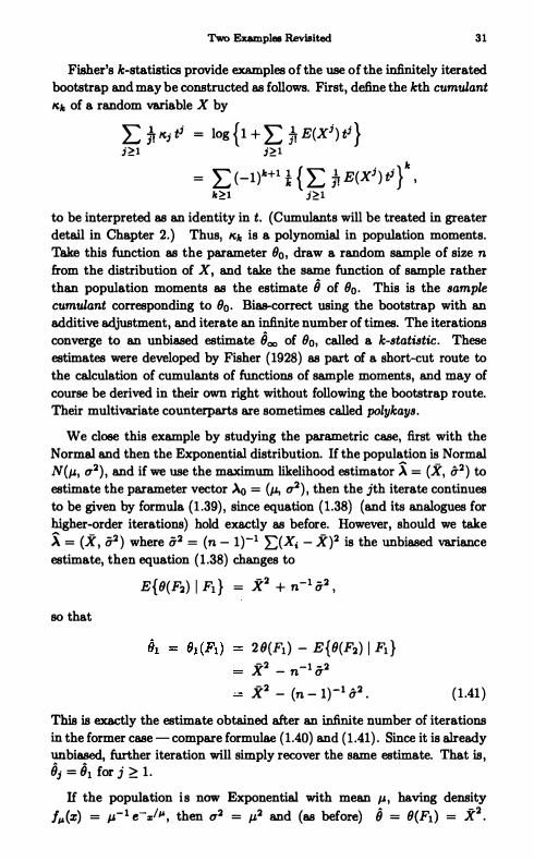
Fisher's k-statistics provide examples of the use of the infinitely iterated bootstrap and may be constructed as follows. First, define the kth cumulant It" of a random variable X by
E � lti ti = log {I + E tr E(Xi} tj } i�1 i�1
= E (-1}"+1 1 { E tr E(Xi} ti }"
, "�1 i�1
to be interpreted as an identity in t. (Cumulants will be treated in greater detail in Chapter 2.) Thus, /tic is a polynomial in population moments.
Take this function as the parameter 80, draw a random sample of size n from the distribution of X, and take the same function of sample rather
than population moments as the estimate 8 of 80• This is the sample cumulant corresponding to 00. Bias-correct using the bootstrap with an additive adjustment, and iterate an infinite number of times. The iterations converge to an unbiased estimate 800 of 00, called a k-statistic. These estimates were developed by Fisher ( 1928) as part of a short-cut route to
the calculation of cumulants of functions of sample moments, and may of
course be derived in their own right without following the bootstrap route. Their multivariate counterparts are sometimes called polykays.
We close this example by studying the parametric case, first with the
Normal and then the Exponential distribution. If the population is Normal N(J.!., 0'2} , and if we use the maximum likelihood estimator :\ = (X, 0-2) to estimate the parameter vector � = (p., 0'2), then the jth iterate continues
to be given by formula (1 .39) , since equation ( 1 .38) (and its analogues for higher-order iterations) hold exactly as before. However, should we take
:\ = (X, (12) where (12 = (n - 1}-1 �(Xi - X}2 is the unbiased variance
estimate, then equation ( 1 .38) changes to
80 that
E{0(F2) I F1} = X2 + n-1 (12 ,
2 9(F1) - E{9(F2} I FI} X2 _ n-1 (12 X2 _ (n _ 1)-1 0-2 . ( 1 .41)
This is exactly the estimate obtained after an infinite number of iterations in the former case - compare formulae ( 1 .40) and ( 1 .41). Since it is already unbiased, further iteration will simply recover the same estimate. That is, 8; = 81 for j � 1 .
If the population is now Exponential with mean J.!. , having density
f,s(z) = J.!.-1 e-c/" , then 0'2 = p.2 and (as before) 8 = 8(Fl) = g2.

32 1. Principles of Bootstrap Methodology
Therefore equation (1 .37) becomes
E{8(Fl) I Fo} = �2 (1 + n-l ) . ( 1 .42) Taking our estimate of "\0 = � to be the maximum likelihood estimate it, we obtain in direct analogy to equation ( 1 .42) ,
E{8(F�) I FI} = X2 (1 + n-1 ) . Therefore one bootstrap iteration produces
81 = 81 (F1) 2 8(F1 ) - E{8(F2) I F1 } = X� (1 - n- 1) .
A second iteration gives
8(Ft } + 81 (F1 ) - E{81 (F2) I FI } g2 + g2 (1 _ n-1) _ g2 (1 + n-1 ) (1 - n-1 ) g2 (1 _ n-1 + n-2) •
Arguing by induction over i we see that after i iterations,
8j = 8j (F1 ) = g2 { 1 _ n-1 + n-2 _ • • • + (_1)i n-j } g2 (1 + n-1)-1 { I + (- l)j n-(j+1) } .
As j --+ 00, 8j --+ 800 = g2 (1 + n-1 )- 1 ,
which is unbiased for 80, Convergence of the infinitely-iterated bootstrap is not a universal phe
nomenon, even in the relatively simple context of bias correction.
Example 1 . 6: Confidence Interval
It follows from Proposition 1 . 1 , or from the fact that Edgeworth expansions are power series in n-1/2 (see Chapter 2) , that in regular cases each bootstrap iteration reduces the order of coverage error by a factor of n-1/2 or less. For two-sided intervals the reduction in order of error is generally greater than this, being a factor of n-1 at each iteration. That follows from the fact that Edgeworth expansions of coverage error of two-sided intervals are power series in n-1 , not n-1/2 (see Chapter 2), and from Proposition 1.2. We open this example by checking condition (1 .30) in Proposition 1 .2. For the sake of definiteness we treat the case of symmetric percentile confidence intervals; other cases, such as equal-tailed intervals, are similar. See Section 3.11 for details.

Two Examples Revisited 33
For symmetric intervals we may take the function h(Ft } to have the form
h(Ft} (Fo , Fl) = I {6(F1) - n-1/2 T(Fl ) � 8(Fo) � 8(Fl ) + n-1/2T(Fl )} - a
= I {nl/2 18(Fl } - 8(Fo) I � T(Fl) } - 0: .
Then
and
e(A) = (8/at) P {nl/2 18(Fl) - 8(Fo) I � U(Fl ' t) I A }Lo . (One possible form for U(" t) is U(· , t) = TO + t.) Employing a Normal approximation to the joint distribution of n1/2{8(Fl ) - 8(Fo )} and A, we see that there exist bivariate Normal random variables (Nt . N2) with zero means and such that
E{ Ae(A)} = E [N2(8/8t) P{ IN1 1 :::; U(Fo , t) I N2}] + O(n-1/2) .
The expectation on the right-hand side equals
(8/at) E [N2P{ IN1 1 :::; U(Fo , t) I N2}]
This verifies (1.30) .
(8/8t) E [N2I{ IN1 1 � U(Fo, t) }] = (8/at) 0
O .
We now discuss the effect that bootstrap iteration has on the two-sided confidence intervals derived in Example 1.2. The nonparametric case is relatively uninteresting at our present level of detail, the main feature being that each successive iteration reduces the order of coverage error by a factor of n-1 . Therefore we confine attention to parametric problems. The parametric intervals developed from pivotal statistics in Example 1 .2 were percentile-t intervals and had perfect coverage accuracy. Iteration of these intervals only reproduces the same intervals. Therefore we focus on nonpivotal intervals, derived by the ordinary percentile method in Example 1.2. It turns out that a single bootstrap iteration of any one of these percentile intervals produces a percentile-t interval having perfect coverage accuracy. Further iterations simply reproduce the same interval.
We begin by recalling from Example 1.2 the parametric, percentile confidence interval for 8 = p., assuming a Normal N(p., (72) population. Let

34 1. Principles of Bootstrap Methodology
N denote a. Normal N(O, l) random varia.ble. Estimate the pa.ra.meter .\0 = (1-', 0'2) by the maximum likelihood estimator
� - · 2 ( 2 ) .>. = (X, 0' ) = 8(Fl) , 0' (Fl ) ,
where X = n-1 E Xi and (;2 = n-1 L:(Xi - X)2 a.re sa.mple mean and sa.mple variance, respectively. The functional It is, in the case of a 95% confidence interval,
h(Fo, Fl) = I {8(Fl ) - t ::; 8(Fo) ::; 8(Ft } + t} - 0.95 ,
and the sa.mple equa.tion ( 1.24) ha.s solution t = T(Fl ) = n-1/2 XO.95 u(F1 ) , where XO.95 is given by P(INI ::; XO.95 ) = 0.95. This gives the percentile interval
( X - n-1/2 XO.95 {; , X + n-1/2 XO.95 (; ) , derived in Example 1.2. For the sake of definiteness we shall make the coverage correction in the form
U(F1 ' t) = n-1/2 (XO.95 + t) u(Ft} ,
although we would dra.w the sa.me conclusion with other forms of correction. Thus,
IU(F1 ,t) (Fo, Ft} = I {n1/2 18(F1 ) - 9(Fo) 1 /O'(Ft } ::; XO.95 + t} - 0.95 ,
so tha.t the sa.mple equa.tion (1.27) becomes
P {n1/2 19(F2) - 9(Fl ) 1 / U(F2) ::; XO.95 + t I Fl } - 0.95
Observe that
W n1/2 {8(F2) - 9(Fd } / U(F2)
O . ( 1 .43)
n n -1/2 {n-1/2 E (X; - X)} { n-1 �:<X; - X)2 } , i=l i=1
where conditional on X, X; , . . . , X; a.re independent and identically distributed N( X, (;2) random va.riables and X· = n-1 L: X; . Therefore conditional on X, and also unconditionally, W is distributed a.s {n/(n - 1)}1/2 Tn-1 where Tn-l ha.s Student's t distribution with n- l degrees of freedom. Therefore the solution to of equa.tion (1 .43) is to = {n/(n _ 1)}1/2 WO.95 - XO.95 , where Will = wllI(n) is defined by
p( ITn-l l ::; Will ) = o . The resulting bootstrap confidence interval is
( 1 /2 • 1/2 • » ) 9(Fl) - n- u(F1) (xO.95 + to) , 9(Fl ) + n- O'(Ft } (XD.95 + tO
= (X - (n - 1)-1/2 wO.95 {; , X + (n - 1)- 1/2 WO.95 (; ) .

Bibliographical Notes 35
This is identical to the percentile-t (not the percentile) confidence interval
derived in Example 1.2 and has perfect coverage accuracy.
Exactly the same conclusion is obtained on iterating the percentile interval constructed in Example 1.2 under the assumption of an Exponential
population: a single iteration produces a percentile-t interval with perfect coverage accuracy. This result does require a special property of both ex
amples, namely, that 9 - 8 can be made exactly pivotal by rescaling, and is not universal in parametric problems.
1 .6 Bibliographical Notes
Before Efron (1979) drew attention to diverse applications of the boot
strap, it existed mainly in disparate, almost anecdotal form, not as a uni
fied, widely applicable technique. Another of Efron's contributions was to marry the bootstrap to modem computational power. He pointed out that many problems which hitherto had not been thought of as avenues for application of the bootstrap, could be tackled via that route if Monte Carlo methods were employed to numerica.1ly approximate functionals of the empirical distribution function. The combined effect of these two ideas
on statistical practice, statistical theory, and statistical thinking has been profound. The reader is referred to Diaconis and Efron (1983) for a detailed and delightfully readable account of computer intensive methods in
statistics.
Others who thought along similar lines include Barnard (1963), Hope (1968) , and Marriott (1979) , who advocated Monte Carlo methods for
hypothesis testing; Hartigan (1969, 1971, 1975) , who used resampled subsamples to construct point and interval estimates, and who stressed the con
nections with Mahalonobis' "interpenetrating samples" and the jackknife of Quenouille (1949, 1956) and Tukey (1958) ; Simon (1969, Chapters 23-25), who described a variety of Monte Carlo methods; and Mantz and Jarrett
(1978), who devised a bootstrap estimate of the variance of the sample median.
Efron's development of the bootstrap, at least insofar as it applies to confidence intervals, diverges from our own almost at the beginning. Efron's account usually stays close to other resampling methods, particularly the jackknife (see, e.g., Gray and Schucany 1972), in its introductory stages. See for example Efron (1979, 198180, 1982, 1987) , Efron and Gong (1983) , and Efron and Tibshirani (1986). Parr (1983) makes a careful analytic comparison of bootstrap and jackknife methods for estimating bias and variance, and Beran (1984b) studies jackknife approximations to bootstrap

36 1. Principles of Bootstrap Methodology
estimates. In comparison, connections with the jackknife do not emerge naturally from our approach. Likewise, the "other percentile method," mentioned briefly in the third paragraph of Example 1.2 in Section 1 .3, does not fit at all well into our set-up, but is basic to Efron's development. It may be justified by a Bayesian argument (Efron (1982, p. 81); see also
Rubin (1981)) . The "other percentile method" is still quite popular among nonstatisticians, and perhaps also with statisticians, who (if those users we know are any guide) seldom employ any corrections such as Efron's (1982, 1987) bias corrections. However, evidence reported by Efron as early as 1980 makes it clear that the uncorrected "other percentile method" can be a poor performer. We doubt that the uncorrected version will survive the test of time, although with appropriate COfTeCtions it may epitomise future directions for bootstrap research; see Section 3.11. Hall (1988&) terms the "other percentile method" the backwards method because it is analogous to looking up the wrong statistical tables ba.ckwa.rds, and ca.lled the ordinary percentile method the hybrid method because it can be interpreted as looking up the wrong tables the right way around.
Our development of bootstrap methodology is similar to that of Hall and Martin (1988a). See also Martin ( 1989). It represents an attempt to find a unified approach that leads canonically to the issues of pivotalness and bootstrap iteration. Those points do not emerge naturally from some earlier accounts. The importance of working with a pivotal statistic when constructing a bootstrap confidence interval, at least in simple situations, is implicit in Hinkley and Wei (1984) and is addressed more explicitly by Babu and Singh (1984) , Hall (1986a, 1988a) , Hartigan (1986) , and Beran (1987) , among others. Pivoting does not always mean rescaling; see Ducharme, Jhun, Romano, and Truong (1985) and Fisher and Hall (1989) for discussions of pivotal statistics that involve spherical data. Our discussion of the sample equation, used to define a bootstrap estimate such as a critical point for a confidence interval, has points of contact with the notion of an estimating equation; see Godambe (1960, 1985) and Godambe and Thompson (1984) for the latter.
The iterated bootstrap is introduced and discussed by Efron (1983) in the context of prediction rules, and by Hall (1986a) and Beran (1987) in the case of confidence intervals. A unified account is given by Hall and Martin (1988a) . See also Loh (1987) , whose method of bootstrap calibration includes bootstrap iteration as a special case.
, Our Russian doll analogy for the iterated bootstrap is reminiscent of Mosteller and Tukey's (1977) "misty staircase" of steps in the construction of successively more elaborate, and more accurate, statistical procedures. After calculating the first and second versions of the procedure, "one should have gone on to a tertiary statistic, which indicated the variability or stabil-

Bibliographical Notes 37
ity of the secondary statistic, then to a quaternary statistic, . . . , and so on up and up a staircase, which since the tertiary was a poorer indicator than the secondary and the quaternary was even worse, could only be pictured as becoming mistier and mistier. In practice, workers usually stopped with
primary and secondary statistics" (Mosteller and Thkey 1977, p. 2) .
Efron (1985) discusses confidence intervals for parametric problems;
Athreya (1987) , Hall (1988c, 199Of), and Mammen (1992) study properties
of the bootstrap when moments are infinite; and Schemper (1987a) describes jackknife and bootstrap methods for estimating variance, skewness,
and kurtosis. General accounts of theory for the bootstrap include Bickel
and Freedman (1981) , Athreya ( 1983), and Beran (1984&). Contributions
to the theory of Edgeworth expansion for the bootstrap, starting with
Singh (1981) , will be recounted at the end of Chapter 3. Further literature on bootstrap methodology will be cited there and at the end of
Chapter 4. Hinkley (1988) surveys bootstrap methods, and DiCiccio and
Romano (1988) describe the state of the art for bootstrap confidence intervals. Work on randomization tests, including material in the monographs
by Edgington (1987) and Noreen (1989), is directly related to bootstrap
methods. Monograph-length expositions of bootstrap methods include Efron (1982), Beran and Ducharme (1991), Mammen (1992), and Efron and Tibshirani (1993) .


2
Principles of Edgeworth Expansion
2. 1 Introduction
In this chapter we define, develop, and discuss Edgeworth expansions as approximations to distributions of estimates 8 of unknown quantities 80 , We call 80 a "parameter" , for want of a better term. Briefly, if 8 is con
structed from a sample of size n, and if n1/2 (8 - 80) is asymptotically Normally distributed with zero mean and variance u2 , then in a great
many cases of practical interest the distribution function of n1/2 (8 - 80} may be expanded as a power series in n-1/2 ,
p{ n1/2 (8 - 80)/u � x} = �(x) + n-1/2pl (X)iP(X) + . . . + n-j/2pj (x)iP(x) + . . . , (2.1)
where iP(x) = (27r)-l/2e-z2/2 is the Standard Normal density function and
�(x) = i: iP(u) du
is the Standard Normal distribution function. Formula (2.1) is termed
an Edgeworth expansion. The functions P; are polynomials with coeffi
cients depending on cumulants of 8 - 80 • Conceptually, we think of the expansion (2 .1) as starting after the Normal approximation �(x) , so that n -1/2 Pl (x) iP( x) is the first term rather than the second term.
The most basic result of this type is in the case where 8 is a sample mean
and 80 the population mean. This example evidences all the main features
of more general Edgeworth expansions: P; is a polynomial of degree at most 3j - 1 and is an odd or even function according to whether j is even
or odd, respectively; and the expansion is valid under appropriate moment and smoothness conditions on the sampling distribution. These properties
are most easily discussed in the context of means, and so that case forms a
convenient introduction. It is given special treatment in Section 2.2, which lays the foundation for more general Edgeworth expansions developed in Section 2.3. For example, we introduce cumulants in Section 2.2. Section
39

40 2. Principles of Edgeworth Expansion
2.3 describes Edgeworth expansions at a formal level, allowing us to give a wide-ranging yet brief account of their applications. Section 2.4 takes up the main issues in more detail and with more conciseness. It describes and analyzes an explicit model under which Edgeworth expansions may be established rigorously.
Equation (2. 1) may be inverted, thereby showing that the · solution x = U", of the equation
admits an expansion
where the P;l 'S are polynomials derivable from the P; 's and z'" is the solution of the equation 4i(z",) = Q. Inverse formulae such as (2.2) are termed Cornish-Fisher expansions, and are described in Section 2.5. Section 2.6 treats examples and gives explicit formulae for some of the polynomials Pi in cases of special interest.
In this brief discussion we have focused on the distribution of the nonStudentized statistic, n 1 /2 (iJ -Bo) / u. But in many cases of practical interest the asymptotic variance u2 would be unknown and estimated by a function q2 of the data. There we would be interested in the distribution function of the Studentized sta.tistic nl/2 (iJ - Bo)/fr. Our treatment will give emphasis to this case, which admits an expansion like (2.1) but with different polynomials Pi ' To distinguish the two types of polynomial we shall wherever possible use Pi for polynomials in the non-Studentized case and qi for polynomials in the Studentized case. This notation will persist throughout the monograph.
The bootstrap will hardly be mentioned during this chapter; we shall allude to it only occasionally, to provide motivation. Thus, the present chapter is quite separate from the previous one. It provides tools for a. theoretical analysis of important aspects of the bootstrap principle, to be conducted in the remainder of the monograph. All our future work will call upon ideas from both Chapters 1 and 2.
We should stress that we are interested in Edgeworth expansions primarily for the light they can shed on theory for the bootstrap. Classical statistical theory employs the expansions to provide analytical corrections rather similar to those that the bootstrap gives by numerical means. Such uses of Edgeworth expansions are incidental to our main purpose, although we shall have a little to say about them in Section 3.8.
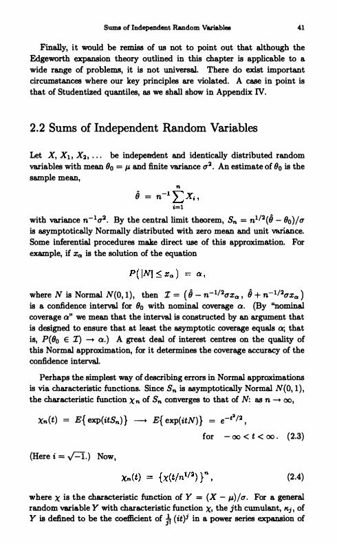
SUID8 of Independent Random Variables 41
Finally, it would be remiss of us not to point out that although the
Edgeworth expansion theory outlined in this chapter is applicable to a
wide range of problems, it is not universal. There do exist important circumstances where our key principles are violated. A case in point is
that of Studentized quantiles, 88 we shall show in Appendix IV.
2.2 Sums of Independent Random Variables
Let X, Xl ! X2 , . . . be independent and identically distributed random
variables with mean 80 = I-' and finite variance u2 • An estimate of 80 is the
sample mean, n . -1 '" 8 = n L.JXi ,
i=1 with variance n-1u2. By the central limit theorem, 8n = nl/2 (fJ - 80)/u is asymptotically Normally distributed with zero mean and unit variance.
Some inferential procedures make direct use of this approximation. For
example, if Xa is the solution of the equation
where N is Normal N(O, 1) , then I = ( fJ - n-1/2uxa , fJ + n-1/2uxa ) is a confidence interval for 80 with nominal coverage a. (By "nominal coverage a" we mean that the interval is constructed by an argument that
is designed to ensure that at least the asymptotic coverage equals ai that
is, P(80 E I) -+ a.) A great deal of interest centres on the quality of this Normal approximation, for it determines the coverage accuracy of the confidence interval.
Perhaps the simplest way of describing errors in Normal approximations is via characteristic functions. Since 8n is asymptotically Normal N(O, 1 ) , the characteristic function Xn of 8n converges to that of N: 88 n -+ 00,
Xn(t) = E{ exp(it8n) } -+ E{ exp(itN)} = e-t�/2 , for - 00 < t < 00 . (2.3)
(Here i = J=I.) Now,
(2.4)
where X is the characteristic function of Y = (X - p,)/u. For a general random variable Y with characteristic function X, the jth cumulant, Iti ' of Y is defined to be the coefficient of � (it)i in a power series expansion of

42 2. Principles of Edgeworth Expa.naion
logX(t) :
X(t) = exp {ltlit + tlt2(it)2 + . . . + fr Itj (itY + . . . } .
Equivalently, since
x(t) = 1 + E(Y)it + tE(y2) (it)2 + . . . + fr E(yi) (it)i + . . . ,
cumulants may be defined in terms via the formal identity
L fr lti (it)j = log {I + L ft E(Yi) (it)i } i�l j�l
= L (-I)k+l t { L ft E(Yi) (it)i }k . k�l j�l
Equating coefficients of (it)i we deduce that
1t1 = E(Y) , 1t2 = E(y2) - (Ey)2 = var(Y) , 1t3 = E(y3) - 3 E(y2)E(Y) + 2 (Ey)3 = E(Y - Ey)3 , 1t4 = E(y4) - 4E(y3)E(Y) - 3 (Ey2)2
+ 12 E(y2) (Ey)2 - 6 (EY)" = E(Y - EY)" - 3(var y)2 ,
and 80 on, the formula for 1t10 containing 41 such terms.
(2.5)
(2.6)
Note that Itj is a homogeneous polynomial in moments, of degree j. Likewise, moments can be expressed as homogeneous polynomials in cumulants, the polynomial for E(yj) being of degree j. Cumulants of multivariate distributions may also be defined; see (2.40) and also part (i) of subsection 5.2.3.
We have standardized Y for location and scale, 80 that E(Y) = 1t1 = 0 and var(Y) = 1t2 = 1. Hence by (2.4) and (2.5) , using the series expansion of the exponential function,
Xn(t) = exp { - !t2 + n-1/2ir 1t3(it)3 + . . . + n-(j-2)/2 fr Itj (it)i + . . . }
= e-t2/2 { 1 + n-1/2r1 (it) + n-1r2(it) + . . .
+ n-j/2rj (it) + . . . } , (2.7)
where rj is a polynomial with real coefficients, of degree 3j, depending on Ita, . . . , 1ti+2 but not on n. This expansion gives a concise account of the rate of convergence in the limit theorem (2.3) .

Suma of Independent Random Variables
One property of the r/s is clear on inspection of the argument leading to (2.7) and will prove crucial in future work: rj is an even polynomial when j is even and is odd when j is odd. It also follows from (2.7) that
(2.8)
and
(2.9)
Many of our arguments involving the bootstrap require only these first two polynomials, and 80 the algebraic details are simpler than might at first appear.
Rewrite (2.7) in the form
x,, (t) = e-t2/2 + n-l/2rl (it)e-t2/2 + n-lr2 (it)e-t2/2 + . . .
+ n-j/2rj (it)e-t2/2 + . . . . (2.10)
Since
and
where � denotes the Standard Normal distribution function, (2. 10) is strongly suggestive of the "inverse" expansion
P(S,, $ X) = �(x) + n-l/2Rl (x) + n-1R2 (x) + " , + n-j/2Rj (x) + . . . , (2.12)
where Ri (x) denotes a function whose Fourier-Stieltjes transform equals rj (it)e-t /2
1: eitz dRj (x) = rj (it)e-t2/2 .
The next step in our argument is to compute Rj .

2. PrincipleB of Edgeworth Expansion
Repeated integration by parts in formula (2. 11 ) gives
e-t2/2 = (-it)-l L: eitz d�(l) (X)
= (-it)-2 L: eitz d�(2) {X)
= (-it)-j i: eitz d�(j) (x) ,
where �(j) (x) = (djdx)j �(x). Therefore
i: eitz d{ (-D)j�(x)) = (it)i e-t2/2 , (2. 13)
where D is the differential operator djdx. Interpret Tj (-D) in the obvious
way 88 a. polynomial in D, so that Tj ( -D) is itself a differential operator.
By (2.13) ,
L: eitz d{Tj {-D)4> (x) } = Tj (it)e-t2/2 ,
and so the function that we seek is none other than Tj (-D)4>(x),
Rj (x) = rj (-djdx) �(x) .
For j � 1 , (-D)j �(x) = -Hej_l (x) tj)(X) ,
where the functions Hej are Hermite polynomials:
Heo(x) = 1 , Hel (X) = x , He2(X) = x2 - 1 , He3 (X) = x(x2 - 3) , He4(X) = X4 - 6x2 + 3 , He5(X) = x(x4 - 10x2 + 15) , . . . .
(2. 14)
See, for example, Magnus, Oberhettinger, and Sani (1966, Section 5.6) , Abramowitz and Stegun (1972, Chapter 22) , and Petrov (1975, p. 137) . They a.re orthogonal with respect to the weight function tj) and are normal
ized so that the coefficient of the highest power in x is unity. Note that
H ej is of precise degree j and is even for even j, odd for odd j. We may
now deduce from (2.8) , (2.9), and (2. 14) that
R1 (x) = -! �3 (X2 - 1) tj){x) and
R2(x) -x{ t. �4(x2 - 3) + ."/2 ��(x4 - 10x2 + 15)} tj)(x) .
For general j � 1 ,

Sums of Independent Random Variables 45
where the polynomial Pj is of degree 3j - 1 and is odd for even j, even for odd j. This follows from the fact that r j is of degree 3j and is even for even j, odd for odd j.
We have just seen that
(2. 15)
and
,Pl(X) = -x{ 2� 1t4(X2 - 3) + i21t�(X4 - 10x2 + 15)} . (2.16)
Formula (2. 12) now assumes the form
P(Sn :5 x) = ib(x) + n-1/2pl (X)t/>(X) + n-1,Pl(x)t/>(x) + . . .
+ n-j/2pj (x)t/>(x) + . . . , (2.17)
called an Edgeworth expansion of the distribution function P(Sn :5 x) .
Third and fourth cumulants 1t3 and It. are referred to as skewness and kurtosis respectively. The term of order n-1/2 in (2. 17) corrects the basic Normal approximation for the main effect of skewness, while the term of order n -1 corrects for the main effect of kurtosis and the secondary effect of skewness.
The expansion (2.17) only rarely converges as an infinite series. Indeed, if X has an absolutely continuous distribution then the type of condition that must be imposed to ensure convergence is E{ exp (� y2) } < 00 (Cramer 1928). This is a very severe restriction on the tails of the distribution of Yj it fails even if Y = (X - J.t)/a when X is Exponentially distributed. Usually (2. 17) is only available as an asymptotic series, or an asymptotic expansion, meaning that if the series is stopped after a given number of terms then the remainder is of smaller order than the last term that has been included,
P(Sn :5 x) = ibex) + n-1/2pl (X)t/>(X) + . . .
+ n-j/2pj (x)t/>(x) + o(n-j/2) . (2.18)
This expansion is valid for fixed j, as n -+ 00. Sufficient regularity conditions for (2. 18) , with the remainder of the
stated order uniformly in all x, are
E( IXIH2) < 00 and lim sup Ix(t) I < 1 . /t /-+oo
The latter restriction, often called Cramtr's condition, holds if the distribution of X is nonsingular, or equivalently if that distribution has a nondegenerate absolutely continuous component - in particular, if X has a proper density function. A proof of this fact in the multivariate case will

46 2. Principles of Edgeworth Expansion
be given at the end of Section 2.4. The reader is referred to bibliographical notes at the end of this chapter for sources of further information.
Thus, our formal inversion of the characteristic function expansion (2. 10) is valid if X has sufficiently many finite moments and a smooth distribution. It fails if the distribution of X is unsmooth, for example if X has a lattice distribution. There, extra terms of all orders, n -1/2, n -1 , . . . , must be added to (2. 17) to take account of the fact that we are approximating an unsmooth step function, peS,. � x) , by a smooth function, the right-hand side of (2. 17). For example, suppose E(X) = 0, E(X2) = 1 , E/X/3 < 00, and X takes only values of the form a + jb, where j = 0, ±1, ±2, . . . and b > 0 is the largest number that allows this property (i.e. , b is the maximal span of the lattice) . Define R(x) = [xl - x+ � , where [xl denotes the largest integer less than or equal to x. Then the analogue of (2.18) in the case j = l is
peS,. :5 x) = �(x) + n-1/2pl {X) ¢(x)
+ n-1/2 bR { (n1/2x - na)/b} ¢(x) + o{n- I/2) ,
for the same polynomial PI as before. (If we strengthen the moment condition on X to E(X4) < 00 then the remainder o(n-1/2) may be replaced by D(n-l ) .) See for example Gnedenko and Kolmogorov (1954, Section 43) .
2.3 More General Statistics
Here we treat Edgeworth expansions for statistics more general than the sample mean. Let S,. denote a statistic with a limiting Standard Normal distribution, such as S,. = nl/2(8 - 8o)/u, or S,. = n1/2 (8 - 80)/iT where iT2 is a consistent estimate of the asymptotic variance u2 of nl/28. Write X,. for the characteristic function of S,., and let Itj,,. be the jth cumulant of S,.. Then
X,.(t) = E{ exp(itS,.) } = exp {tel ,,.it + �1t2,n (it)2 + . . . + � Itj,n {it)j + . . . } j (2.19)
compare (2.5) .
In many cases of practical interest, Itj,n is of order n-(j-2) /2 and may be expanded as a power series in n -1 :
-(j-2)/2 (k + -lk + -2k + ) lej,n = n i,l n i,2 n j,3 . • • , j � 1 , (2.20)
where kl,l = 0 and k2,l = 1. The latter two relations reflect the fact that S,. is centred and scaled so that tel,,. = E(Sn) -- 0 and 1£2, .. = var(S,.) -- 1 .

More General Statistics 47
When 8" is a normalized sum of independent and identically distributed random variables, formula (2.20) is implicit in the first identity of (2.7), which declares that
-(j-2)/2 It - = n Itj ,," , j � 2 , (2.21)
where Itj is the ith cumulant of Y. In its full generality, (2.20) is a deep result with a rather involved proof. Section 2.4 will give a proof of (2.20) under a model where Sn is a smooth function of vector means.
Combining (2. 19) and (2.20) we see that
X,,(t) = exp [ - !t2 + n-l/2 {kl,2it + fr k3.1 {it)3 }
+ n-1 { lr k2•2 {it)2 + if k" l (it)4} + . . . ] = e-tl/2 (I + n-l/2 {kl.2it + ! k3.1 (it)3 }
+ n-1 [!k2.2 (it)2 + i4 k4•1 (it)' + l {k1,2it + 1 k3,l (it)3 } 2] + O(n-3/2») . (2.22)
More generally, (2.19) and (2 .20) give
Xn(t) = e-el/2 + n-1/2rl (it)e-el/2 + n-1r2 (it)e-el/2 + . . .
+ n -;/2rj( it)e-el /2 + . . . ,
where rj is a polynomial of degree no more than 3i, even for even i and odd for odd j. This expansion is formally identical to (2. 10), the latter derived in the special case where S" was a sum of independent random variables. The expansion may be inverted, as described in Section 2.2, to produce an analogue of the Edgeworth expansion (2. 17),
P(S" � z) = �(z) + n-1/2pI (Z)q.,{Z} + n-1P2{z)t/>(z) + . . .
+ n-j/2pj (x)q.,{z) + . . . , (2.23)
where Pi is a polynomial of degree no more than 3j - 1, odd for even j and even for odd j. We call PI a skewness correction and 1'2 a correction for kurtosis and for the secondary effect of skewness, even though interpreta.tion of skewness and kurtosis may be rather different from the case of sums of independent random variables.
Recall from the previous section that
L: eitz d{ -Hej_l (z)q.,{x)} = (it)je-e2/2 , j � 1 ,

48 2. Principles of Edgeworth Expansion
where H ej is the jth Hermite polynomial. From this fact, and since by (2.22) ,
Tl (it) kl.2it + � k3•1 (it)3
and
T2 (it) = Hk2,2 + k�.2) (it)2 + i4 (k4,1 + 4k1,2k3, l ) (it)4 + -i2 k�,l (it)6 ,
we have
and
1'2(x) = -{ Hk2.2 + k�.2)Hel (x) + -h (k.,l + 4k1,2k3, l )He3(X)
+ � k�.lHe5 (x)} = -x{ � (k2,2 + kt2) + -h (k4•1 + 4k1,2k3,l) (X2 - 3)
+ -i2 k�,l (x4 - 10x2 + 15)} . (2.25)
As was the case in Section 2.2, expansions such as (2.23) usually do not converge as infinite series but are available as asymptotic expansions or series, meaning that
for j � 1. In the next section we shall develop a concise model for S", with explicit regularity conditions under which this expansion is available uniformly in x.
We motivated our study of Edgeworth expansions in Section 2.2 by pointing out that they may be used to describe coverage accuracy of confidence intervals, among other things. We shall close the present section by illustrating applications. Suppose first that the statistic S" is S" = nl/2 (fJ - (Jo)/a, where a2 denotes the asymptotic variance of nl/2fJ. Then, nominal a-level confidence intervals for (Jo are
where Xa and %a are defined by
P( INI :c:; xa) = a and P(N :C:; %a) = a ,
and where the random variable N has the Normal N(O, 1) distribution. Remembering that odd/even indexed P; 's are even/odd functions respectively,

More General Statistics 49
we see from (2.23) that the actual coverage probabilities of these intervals
are
and
P(80 E II) = P(80 < fJ + n-I/20'Za) = P(Sn > -zoo) = 1 - {.(-Za) + n-I/2Pl (-Za)tP(-Za) + O(n-l ) }
Q - n-1/2Pl (Za)tP(Zo) + O(n-I)
P(Sn > -Xa) - P(Sn > Xa) P(Sn $ X.,) - P(Sn $ -X.,)
= .(Xa) - .( -Xa) + n-1/2 {Pl (Xa)tP(Xa) - PI (-X.,)tP(-x.,) }
+ n-1 {P2 (X.,)tP(xa) - P2( -X.,)tP( -X.,) } + n-a/2 {pa (Xa)tP(Xa) - Pa ( -X.,)tP( -X.,) } + O(n-2)
= Q + 2n-1P2 (xa)tP(Xa) + O(n-2) .
(The function tP is of course even.) Thus, one-sided confidence intervals
based on the Normal approximation have coverage errors of order n-1/2 , whereas two-sided intervals have coverage errors of order n-1 , without any
adjustment or correction.
The same argument shows that
and
P(80 E It} = Q + 2:>-j/2 ( -l)jpj (z.,) tP(Z.,) j�l
P(80 E I2) = Q + 2 Ln-jP2j (xa) tP(xa) , j�1
where both expansions are to be interpreted as asymptotic series. Thus, the coverage probability of one-sided confidence intervals is a series in n-1/2 , whereas that for a tw�sided interval is a series in n -1 . This fact has
important ramifications for bootstrap iteration, since it means that each
iteration reduces the order of error by a factor n-1/2 in the case of one
sided confidence intervals, but by n -1 in the case of two-sided intervals.
See Example 1 .6 in Chapter 1 and Section 3.1 1 for further details.
These results are consequences of a property that is of such major importance it is worth repeating: odd/even indexed Pj '8 are even/odd functions, respectively. When this property fails, results and conclusions can be very different from those described here; see Appendix IV.

50 2. Principles of Edgeworth Expa.naion
H 0- is unknown then we may estimate it by iT, say. In this case we work with 8n = n1/'l (8 - 8)/iT instead of n1/2 (8 - 8)/0-. This new Sn admits the same expansion (2.23) , but with different polynomials. We shall denote them by q instead of P; Section 2.6 will give examples of the differences between Pi and qj . Thus,
p{ n1/'l(8 - (0)/iT � x} = �(x) + n-1/2q1 (X)f/>(X) + . . . + n-j/2qj (x)f/>(x) + . . , ,
where again odd/even indexed q/s are even/odd functions, respectively. Examples of on&- and two-sided confidence intervals are
.11 = ( - oo , 8+n-1/'liTzQ) and .12 = (O-n-1/2iTxQ , 8+n-1/2iTxQ) ,
respectively. Both have nominal coverage o. The results on coverage probability stated earlier for II and I2 continue to hold for .11 and .12, except that the p's are now replaced by q's. For example,
and
j2:.1
P(80 E .12) = 0 + 2 Ln-iq2i (XQ)f/>(xQ) 12:.1
o + 2n-1q2 (xQ)f/>(xQ) + O(n-2) .
Edgeworth expansions may be applied to other functionals of the distribution of 8. For example, to obtain expansions of moments observe that if r � 1 is an integer and we define 8n = n1/2 (8 - 8)/u, then
E{(8 - Bt} = (n-1/'lo-t E(S�)
= (n-1/2ut { lOO xr dP(Sn � x) - lOO
(-xt dP(8n � -x)} = (n-1/20-tr 100 xr-1 { P(Sn > x) + (-ltP(8n � -x)} dx ,
on integrating by parts to obtain the last line. When r is even,
P(8n > x) + (_l)r P(Sn � -x) = P(INI > x) - 2 L n-iP2i (x)f/>(x) ,
and when r is odd,
P(8n > x) + (-ltP(Sn � -x)
j?: l
_2n1/2 L n-jP2j-l (x)f/>(x) . j�l

More General Statistics
Hence
E{(0 - 8r} =
(n- 1/2ur{E(JVf') - 2r L n-j LJIO Xr-1P2j (X)¢(X) dx} j�1 0
for even r,
_2r(n-1/2u)rn1/2 E n-j 1010 Xr-1P2j_1 (X)¢(X) dx j�l 0
for odd r.
These formulae may be combined as
E{ (0 - 8t} = n-[(r+l)/2] (Cl + c2n-1 + can-2 + . . . ) ,
51
(2.26)
where [xl denotes the largest integer less than or equal to x and the constants Cl , C2 , " " depending on r, are determined by polynomials in the Edgeworth expansion for S... (The fact that these expansions of moments are series in n -1 was used in Section 1.4 to explain the performance of bootstrap iteration in problems of bias reduction. It implies that each iteration reduces the order of error by a factor n -1 , not n -1 /2 .)
Formulae for absolute moments may also be obtained in this way. If r > 0, not necessarily an integer, then
As in previous expansions, the infinite series here and in (2.26) are to be interpreted as asymptotic series.
A rigorous proof of these results via this route requires a nonuniform (or weighted uniform) estimate, of the form
_oos��
<oo ( 1 + Ix l) ' lp(S .. � x) - {�(x) + t n-lc/2plc (X}¢(X) } I
= O(n-(J+l)/2)
for large I, of the difference between P(S .. � x) and its Edgeworth expansion up to the jth term. Such results may be readily derived, but expansions such as (2.26) are often available more generally than are the Edgeworth expansions from which they were obtained. For example, if 80 denotes a population mean and fJ the corresponding sample mean, and if rth order population moments are finite, then result (2.26) holds without any additional assumptions on the population (e.g. , without Cramer's condition) . In this case, each series contains only a finite number of nonzero terms. It is for reasons such as this that during most of this monograph we shall

52 2. Principles of Edgeworth Expanaion
work only formally with Edgeworth expansions, without giving absolutely rigorous proofs. (Chapter 5 is an exception. ) There is every expectation that many of our results are available under conditions considerably more general than those we would have to impose to obtain rigorous proofs using presently available technology. Sometimes, as in the example of moments of the sample mean, the natural method of proof is not via Edgeworth expansions, but nevertheless that route does serve to unify, explain, and even motivate the results.
2.4 A Model for Valid Edgeworth Expansions
In this section we describe a general model that allows formulae such as
the cumulant expansion (2.20) and the Edgeworth expansion (2.23) to be established rigorously. Let X, Xl , X: h . . . be independent and identically distributed random column il-vectors with mean "', and put X = n-l r: x.. Let A : lRG -+ lR be a smooth function satisfying A(",) = O. We have in mind a function such as A(x) = {g(x) - g(",H/h(",), where 80 = g(l') is
the (scalar) parameter estimated by iJ = g(X) and h(",)2 is the asymptotic variance of nl/2iJj or A(x) = {g(x) -g(",)}/h(x) , where heX) is an estimate of h(",) . (Thus, we assume h is a known function.)
This "smooth function model" allows us to study problems where 80 is a mean, or a variance, or a ratio of means or variances, or a difference of means or variances, or a correlation coefficient, etc. For example, if {WI , ' " , Wn} were a random sample from a univariate population with mean m and variance (32 , and if we wished to estimate 80 = m, then we would take d = 2, X = (X(I) , X(2» )T = (W, W2)T, #.I. = E(X) ,
This would ensure that g(l') = m , g(X) = W (the sample mean), h(l') = (32, and
n = n-I E (w, - W)2 = /32
'=1 (the sample variance) . If instead our target were 80 = (32 then we would take d = 4, X = cw, W2, w3, W�)T, '" = E(X) ,
g(X(l) , . . . , X(4» = X(2) _ (X(I» ) 2 , h(x(l) , . . . , x(4» = x(�) - 4x(l)X(3) + 6 (x(1» 2X(2)
_ 3 (x(l» � - {:z;(2) _ (x(l» 2}2 .

In this C88e,
A Model for Valid Edgeworth Expansions
g(J.I.) = {32 , g(X) = jP , h(J.I.) E(W - m)4. - rr ,
.. heX) n-1 L (Wi - W)2 - � .
1=1
53
(Note that E(W - m)4. - (34 equals the 8Bymptotic variance of n1/2 /J2 .)
The cases where 80 is a correlation coefficient (a function of five means) , or a variance ratio (a function of four means) , among others, may be treated similarly.
Denote the ith element of a d-vector v by veil or (V)(I) , and put
Z = n1/2 (X - J.I.) and
Bi . = (1Ji/8x(h) . . . 8x(lj » A(x) I . (2.21) 1 . · •• j x=,.
By Taylor expansion, and since A(J.I.) = 0 and Z = Op(l),
where the Op notation is defined on p. xii, and d d d
S .. r = L BiZ(I) + n-1/2 i L E Bi1 1, Z(it } Z(la ) + . . . i=1 i1=1 ia=1
(2.28)
1 d "
+ n-(r-l)/2 _ '" ' " '" n.. . Z(11) . • . Z(ir) • (2.29) , L..J L..J ... i · · ··r r. il=1 ir=1 The following theorem declares that the cumulants of S .. r admit the ex
pansion (2.20) .
THEOREM 2 . 1 . Let Z = n1/2 (X - J.I.), where X denotes the mean of
n independent random vectors distributed 8B X, with finite jrth moments
and mean J.I.. Put
d " " U .. r = L:)iZ(i) + n-1/2 L L biti, Z(11 )Z(I') + . . .
i=1 11 =1 .,=1 " d
+ n-(r-l)/2 '" • • . '" b. Z(i, ) . . . Z{ir) L..J L....J 11 • • • lp ,
for arbitrary but fixed constants b. Then the jth cumulant of U .. r h8B the
form
It; .... r = n-U-2)/2 ( lei.1 + n-11ej,2 + n-2ki,3 + . . . ) ,
where the constants lei,l depend only on the b's, on the moments of X up to the jrth, and on r, and where the series contains only a finite number

2. Principlell of Edgeworth Expamion
(not depending on n) of nonzero terms. The values of kj,l for I � r + 2 - j do not depend on r .
A proof will be given towards the end of this section.
Assume that the first j moments of the O,,(n-r/2) term in (2.28) are all of order n-r/2 , which is guaranteed under moment conditions on X and mild assumptions about A. Then the jth cumulant ltj,,, of S" equals the jth cumulant of S"r plus a remainder of order n-r/2 •1 The latter may be made arbitrarily small by choosing r sufficiently large. Arguing thus it can be seen that It;,,, admits the expansion (2.20) , interpreted as an asymptotic series rather than an infinite series. (See Section 2.2 for a definition of an asymptotic series.)
Result (2.20) was the main requirement for our formal derivation of the Edgeworth expansion (2.23) in the previous section. Theorem 2.2 below gives explicit regularity conditions, assuming the above model for S", under which (2.23) is valid as an asymptotic series. Before passing to that theorem we should compute the asymptotic variance of S", so that we may rescale to ensure that S" has unit asymptotic variance. The latter assumption is implicit in (2.23) . We should also calculate formulae for the coefficients in the polynomial Pl .
Put
Then lJi = 0 for each i ,
E(Z(i) ZW) lJij , E(Z(i)ZWZ(1c» = n-1/2IJij/c ,
and
Take r = 2 in (2.28) , so that it becomes
d d d S" = E /liZ(i) + n-1/2 i E E /lijZ(i) Z(j) + Op(n-I ) .
i=1 i=1 ;=1
(2.30)
IThis is a slight oversimplification, since in principle it may happen that B(18 .. li) is not even finite, whereas B(lS .. r li ) is finite. The point is that in a limit theorem for probabilities, &8 distinct from momenta, it is neceeeary only to note that Sft .. approximates S .. with an error of Op(n-r/'), not that the momenta (or cumulanta) agree to this order. Our formal manipulation of cumulanta aerves only to determine the detaila of the approximation of Sft .. to S ... .

Then
and
A Model for Valid Edgeworth Expansions
d d n-1/:1i E E a'j!Jij + O(n-l ) ,
i=1 j=1 d d
E E aoaj/l'j + O(n-l ) , .=1 j=1
The first three cumulants of Sn are thus
/Cl,n = E(Sn) = n-1/:1 Al + O(n-l ) ,
/C:1,n E(S!) - (ESn? = (1:1 + D(n-l ) ,
and
/C3,n E(S!) - 3E(S;)E(Sn) + 2(ESn)3 = n-1/2 A2 + D(n-l ) ,
where d d
55
(12 = E E aoaj/l'j • (2.31) .=1 j=1
d d Al i E L: aoj/Jij , (2 .32)
i=1 j=1 d d d d d d d
A2 E E E aoajak/Jijlc + 3 E E L: E aoajakl!Jik/Jjl . (2.33) .=1 j=I Ir=1 .=1 j=1 10=1 /=1
In particular, the asymptotic variance of 8n is (12 . If (1 does not equal unity then we should redefine Sn = n1/2 A(X)/(1. For this definition of Sf'U the constants k1,2 and k3t! appearing in formula (2.24) for PI (x) are
and
This follows from the calculations in the previous paragraph, noting formula (2.20) for /Cj,n.

56 2. PriDcipies of Edgeworth Exp&llllion
Given a d-vector t = (t(l) , . . . , t(d» )T , define
and
d X(t) = E{ exp (i E tU) X(j») } .
j=1
THEOREM 2.2 . Assume that the function A has j +2 continuous derivatives in a neighbourhood of I-' = E(X), that A(I-') = 0, that E(I IXllj+2) < 00, and that the characteristic function X of X satisfies
lim sup Ix(t) 1 < 1 . IIt l l-co
(2.34)
Define a'l . . . ir and IJh ... ir by (2.27) and (2.30) , and 0', AI, and A2 by (2.31)-(2.33). Suppose 0' > O. Then for j � 1 ,
P{nl/2A(X)/u � x} = �(x) + n-1/2PI (X)4>(X) + . . .
+ n-j/2pj (x)4>(x) + o(n-j/2) (2.35)
uniformly in x, where Pj is a polynomial of degree at most 3j - 1 , odd for even j and even for odd j, with coe1Iicients depending on moments of X up to order j + 2. In particular,
A proof of this result follows straightforwardly from an Edgeworth expansion of the d-.variate distribution of Z = n1/2 (X - 1-') , as follows. It may be proved that under the conditions of Theorem 2.2,
j p(Z E R.) = E n-Ic/2 PIc (R.) + o(n-j/2)
k=O
uniformly in 8- large class of sets R. � Rd, where the Pk'S are (signed) measures not depending on n and Po is the probability measure of a Normal random variable with zero mean and the same variance matrix as X. See Lemma 5.4 for a concise statement of this result. Taking
'R. = 'R.(n, x) = {z E IRd : nl/2 A (I-' + n-I/2 z) � x} , -00 < x < 00 ,
we obtain immediately an expansion of P{nl/2 A(X)/u � x}. This may be put into the form (2.35) by Taylor expanding the function p,,{R.(n, x)} about Pk{R.(OO, X)} , for 0 � k � j. Details of this argument are spelled out in part (iii) of subsection 5.2.3. Bhattacharya and Ghosh (1978) give a proof of Theorem 2.2 that follows just this route.

A Model for Valid Edgeworth ExpansiOllll 67
Condition (2.34) is a multivariate form of Cramer's continuity condition. It is satisfied if the distribution of X is nonsingular (i.e. , has a nondegenerate absolutely continuous component) , or if X = (W, W2, • • • , Wd) T
where W is a random variable with a nonsingular distribution. See the end of this section for a proof. Cramer's condition implies that any atoms of the distribution of X have exponentially small mass, 80 that the distributions of statistics such as n1/2 A(X)/O' are virtually continuous. The following result is derived at the end of the section.
THEOREM 2.3 . If the distribution of X satisfies (2.34) then for some E > 0,
sup P(X = x) = O(e-En) xEIR"
as n -+ 00.
The resd.er will recall that at the beginning of the section we suggested that the asymptotic variance of an estimator fJ = g(X) of the parameter 80 = g(p.) might be taken equal to a function 7'2 of the mean p., and might be estimated by the same function of X. We now verify that this is possible. If A(x) = g(x) - g(p.) then by (2.31) ,
d d 0'2 = LL9(i) (P.)gU) (p.) {E(X(i)XU» _ jj(i)jjU) } ,
i=l j=l where 9(i) (x) = (8/8x(i» g(X) . Suppose we sd.join to the vector X all those
products X(i) X(j) that are such that 9(i) (x)g(j) (x) is not identically zero and that do not alresd.y appear in X, and sd.join analogous terms to the vectors Xi and X. Let p. denote the mean of the new, lengthened X, and put X = n-1 EXi. Then u2 is assuredly a function of p, say h2(p.), and is estimated vIn-consistently by h2(X) . Values of 0'2 computed for the functions
B1 (x) = {g(x) - g(p.)} / h(p.) and B2(x) = {g(x) - g(p)} / h(x) , in place of A(x) , are both equal to unity. See Section 2.6 for specific examples of this type.
Observe that g(p.) equals a functional 8(Fo) of the population distribution function Fa. In all cases of the nonparametric bootstrap applied to estimation of this 8(Fo) , and in many parametric examples, g(X) = 8(Fl ) where Fl is the sample distribution function, defined in Section 1 .2. This means that if 8 is defined by e = g(X) then 8 = 8(F1 ) , 80 that our model fits into the bootstrap framework developed in Chapter 1. That will prove important in Chapter 3 when we develop Edgeworth expansions in the context of the bootstrap.

58 2. Principles of Edgeworth Expa.naion
The main thrust of work in this section has been to derive Edgeworth expansions for distributions of statistics of the type A(X) , where the function A does not depend on n. The latter condition ma.y be removed, although then the form of the results can change. Some work in la.ter chapters will be directed towards functions An of the type
An(x) = Bo (x) + n-1/2B1 (x) + . . . + n-m/2Bm(x) , (2.37)
where m � 0 is fixed and Bo, Bl , . . . , Bm satisfy the conditions previously imposed on A. In particular, we ask that Bic not depend on n and that BIc (I') = 0 for 0 � k � m. When An has this form, cumulants of the statistic Sn may no longer enjoy the key property (2.20). The reason is that if odd-indexed Bi 's are not identically zero, then in a Taylor expansion of Sn of the form (2.28) , (2.29) it may no longer be true that the coefficient of n-i/2 for odd/even j is always 8880ciated with a product of an even/odd number of Z(il 's, respectively. Instead, with Z = n1/2 (X - 1') we have
where b · · . = (8kj83;<ttl . . . 8x(i.» B · (x) I . .1.·1 · · ··. .1 x=,.
This means that the cumulant expansion on the right-hand side of (2.20) now decreases as a power series in n-l/2 rather than n-1 • However, the leading term is still of order n-U-2l/2, as may be seen by reworking the proof of Theorem 2.1 which we shall give shortly.
Thus, when the function A = An has the form (2.37) , expansion (2.35) in Theorem 2.2 continues to hold if the conditions imposed earlier on A are now required of Bo, . . . , Bm. However, the polynomial Pi in (2.35) can no longer be guaranteed to be odd/even for even/odd j, respectively. Therefore some of the results outlined at the end of Section 2.3 will no longer be valid.
In practice this causes no difficulty, for the following reason. It turns out that we are interested in expansions of
p{ nl/2 An(X) � x}
= P [nl/2{ Bo(X) + n-1/2 Bl (X) + . . . + n-m/2 BmCX)} 5 x] (2.39)
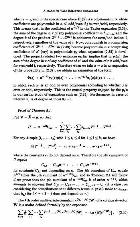
A Model for Valid Edgeworth Expll.llllioDS 59
when z = z, and in the special case where Bj (x) is a polynomial in x whose coefficients are polynomials in z, all odd/even if j is even/odd, respectively. This means that, in the coefficient of n-I/2 in the Taylor expansion (2.39), the sum of the degree in z of any polynomial coefficient in bj,i . . . ... and the degree k of the product Z(id . . . Z(i. } is odd/even for even/odd indices " respectively, regardless of the value of j. Now, polynomials in z comprising coefficients of Z(i. } • • • Z(i.} in (2.39) become polynomials in z comprising coefficients of zr (say) in polynomials Pj when expansion (2.35) is developed. The property stated two sentences earlier implies that in PI (Z), the sum of the degree in z of any coefficient of zr and the value of r is odd/even for even/odd ', respectively. Therefore when we take x = z in an expansion of the probability in (2.39) , we obtain an expansion of the form
�(z) + n-1/2'11"l (Z)t!>(Z) + . . . + n-j/2'11"j (z)t!>(z) + . . . , in which each 'll"j is an odd or even polynomial according to whether j is even or odd, respectively. This is the crucial property enjoyed by the Pj 'S in our earlier study of expansions such as (2.35). Furthermore, in cases of interest 'll"j is of degree at most 3; - 1.
Proof of Theorem 2.1.
Put V = X - I', 80 that
r
L L ' " L b'l . . . '. Veil ) • . • V(i.) . Ie=l il i.
For any k-tuple (il l . . . , ile ) with 1 :5 il :5 d for 1 :5 I :5 k, we have
where the constants Cj do not depend on n. Therefore the jth cumulant of U equals
C + C -1 + + C -;r+1 ;,1 j.2n . . . j,jrn , for constants Cj•1 not depending on n. The jth cumulant of Unr equals
nj/2 times the jth cumulant of n-1/2Unr , and 80 Theorem 2.1 will follow if we prove that the jth cumulant of n-1/2Unr is of order n-;+1 , which amounts to showing that Cj•1 = Cj•2 = . . . = C;.;-1 = O. (It is clear, on considering the contributions that different terms in (2.29) make to tej.n.r , that kj.1 for I :5 r + 2 - j does not depend on r.)
The kth order multivariate cumulant te(h . . . . . i. } (W) of a column a-vector W is a scalar defined formally by the expansion
L lr E . . · E t(il } • • . t(i· )te(i· ·· · · ··· } (W) = log {E(etTW)} , (2.40) '�l " ill

60 2. Princlplllll of Edgeworth Expansion
where t = (t(l) , . • • , t(d) T. Of course, the right-hand side here equals
log {I + :E if L ' " L t(i, ) . • • t(ill) E(W(i. ) . . . W(ill» }
•
"�l il i.
The identity (2.40) should not be interpreted as requiring that W have a proper moment generating function; it is intended to give only a formal definition.
An equivalent definition in alternative notation may be given as follows. Suppose the index I appears precisely il times in the vector (it, . . . , i,,). Define
�(j J' ) - �(il o" . • ilo) (W) "' 1 0 l, . . • - .� , (2.41)
valid since the right-hand side depends on iI , . . . , i" only through iI , i2, . . . .
Put
J,£(jI , j2 , . . . ) = E(W(it } . . . W(i.») ,
1'(0, 0, . . . ) = 1 and K,(O, 0, . . . ) = 1 .
Then equation (2.40) 8B8umes the form
'" . . (t(l» jl (t(l» ja . . . L..J K,(jl t J2, . . . ) . , . I
31 .3a.. . . Jl ·Jl· · · .
{ '" . . (t(l» jl (t(2» h . . . } = log L..J J.'(j1 . J2, . " ) . , . , . . . JI ·Jl . . . .
.1 1 ,32 , · · ·
List the terms
V(l), . • • , V(d), V(l)V(I), V(I)V(2), . . . , V(d) V(d), V(I) V(l)V(l), . . • , (V(d» ,.
as 8. vector W, and the terms
as a vector B. Then U = Ei B(i) W(i) , 80 that
E(U") = L · · · :E B(il ) • . • B(i.) E(W(it l . . . W(ir.» ) . il ir.
Let K,,(U) denote the kth cumul&nt of U. Since cumul&nts are homogeneous polynomials in moments,
K,,(U) = :E . . . E B(it l . . . B(i. )K,(il . . . . ,i.) (W) . il i.
Therefore our proof of Theorem 2.1 will be complete if we show that whenever k � 1 and il , . . . , i" � I,
(2.42)
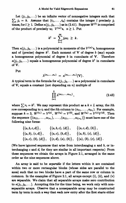
A Model for Valid Edgeworth Expansions 61
Let (jl ,h , . . . ) be an infinite vector of nonnegative integers such that
Ei ii = k. Assume that (i l l ' " , i,, ) contains the integer l precisely il times, for I � 1. Define 1C(j1 l h, . . . ) as in (2.41) . Suppose W(I} is comprised
of the product of precisely WI v(a) ,s, a � 1. Put
00 kt = Lilwi � k .
1=1
Then 1C(jI , i2 , " ' ) is a polynomial in moments of the v(a) ,s, homogeneous and of (precise) degree kt . Each moment of V of degree b (say) equals a homogeneous polynomial of degree b in cumulants of V. Therefore 1C(jI ,h, . . . ) equals a homogeneous polynomial of degree kt in cumulants of V.
Put >.(a1 • . . . • a� ) = lC(a1 • . . . . a� ) (v) .
A typical term in the formula for 1C(j1 ,h, . . . ) as a polynomial in cumulants of V, equals a constant (not depending on n) multiple of
L II >. (an • . . . • al�l ) , (2.43) 1=1
where E rl = kt . We may represent this product as a k x L array, the lth row corresponding to il and the lth column to (al l , . . . , alrl ) ' For example, suppose k = 3, W(id = V(4) , W(i2) = V(b) , and W(ia) = V(c) V(tl) . Then the sequence { (aLl , ' " , alr1 ) , . . . , (aLl , . . . , aLrL ) } must have one of the following nine forms:
{ (a, b, c, d) } ,
{ (a, b) , (c, d) } ,
{ (a, c) , (b) , (d) } ,
{ (a, b, c) , (d) } ,
{ (a, c) , (b, d) } ,
{ (c, d) , (a) , (b) } ,
{ (a, c, d) , (b) } ,
{ (a, b) , (c) , (d) } ,
{ (a) , (b) , (c) , (d) } .
(We have ignored sequences that arise from interchanging a and b, or in
terchanging c and d, for they are similar in all important respects.) From these sequences we obtain the arrays in Figure 2.1 , arranged in the same order as the nine sequences above.
An array is said to be separable if the letters within it are contained within two or more rectangular blocks (whose sides are parallel to the axes) such that no two blocks have a part of the same row or column in common. In the examples of Figure 2.1 , all arrays except (i) , (ti) , and (v) are separable. We claim that all separable arrays make zero contribution to 1C(jI , j2 , " ' ) ' Accepting this for the time being, we work only with nonseparable arrays. Observe that a nonseparable array may be constructed term by term in such a way that each new entry after the first starts either

62 2. Principles of Edgeworth Expaoaion
(i) . • (ii) :
Lb (iii) a
L (Iv)
(vii)
b b cd cd
I abed
a
L b b cd cd
ab cd
a
L b b cd c d
8C b d
cd c d abc d
(v) a
L b b cd e d
8C bd
(Viii) 8
L b b cd cd
cd a b
(vi)
b b cd cd
acd b
a
L b b cd c d
ab c d
(iX) 8
L b b cd c d
8 b c d
FIGURE 2 . 1 . Arrays constructed from the nine consecutive sequences {(a, b, c, d)}, . . . , Ha) , (b) , (c) , (d)}.
a new row, or a new column, or neither, but not both. Hence if there are R rows, C columns, and L letters in the nODBeparable array,
L � 1 + (R - 1) + (C - 1) = R + C - l . (2.44)
Since V is a centred sample mean then the argument leading to (2.21) may be easily modified to show that the cumulant A (al o ' " .ar) , corresponding to a vector (a, b, . . . ) of r letters, is of order n-( .. -l) as n -+ 00 . Therefore the product at (2.43) is of order n-II , where
1/ = all vectors(ll.b, . . . ) repr_ntlng
columns iD an array
total number of letters
= L - C � R - 1 ,
(number of letters - 1)
number of columns
using (2.44). But R = k, and so the order of each term in II:( .. . · · · .·�) (W) can be no greater than n-{lc-l) . The number of terms does not depend on

A Model for Valid Edgeworth ExplUlllions 63
n, whence
This proves (2.42) .
It remains to prove the claim made two paragraphs earlier, that separable arrays make no contribution to ItUl t h , . . . ) = It(il • . . . • i2) (W). This we do by induction over k. The claim is trivially true when k = I, for there are no separable arrays in that case. Given that the claim is true for all orders up to and including k - 1, we shall prove it for k.
Put
and (as before) >.(01 • . . . • Or) = ItC01 • . . . • Q:r) (V) . Formula (2.40) gives
"'(i1 • . . . • i.) = E E It(flll • . . . • fllo1 ) . . • 1t(flGl •. . . • fl .. o .. ) , (2.45)
where the outer sum is over all a � 1 and all 81, ' " , Sa such that 81 + . . . + 8a = k and the inner sum is over all distinct terms obtained by permuting (i 1 , . . . , i,,) to (P11 , " • , Phl ' 1321 , . . . , [jaB .. ) ' The only term on the right-hand side of (2.45) involving only a single cumulant is It(il ; . • • • i. ) . Therefore we may rewrite (2.45) as
and hence
(2.46)
where K stands for the sum of products of two or more cumulants of the form It(i� • . . . • i�I ) , with k' � k - 1. By the induction hypothesis, no terms arising from separable arrays make contributions to K. Therefore it suffices to prove that if any term arising from a separable array makes a contribution to "'(i1 • • • • • i.) then it cancels from the difference "'(i1 • • • • •
i. ) - K. Consider an array of the type introduced below (2.43), with rows de
termined by (il l . . " ilc) and columns by vectors 01 = (all, . . . , Olrl ) ' 1 � l � L. Suppose the array is separable into B nonseparable blocks. Without loss of generality, the bth block has its rows determined by
and its columns by vectors 0"1+" '+".- 1+1 , . . . , O"' +" '+"h ' as indicated in Figure 2.2. Of course,
and L .

64 2. Principles of Edgeworth Expansion
The entire array represents the product
L � = II ,\QI
1=1
appearing in an expansion of It(" ' · · · ,'· ) . We shall prove in the next par8r graph that the coefficient of � in J.t(i" . • • • i.) equals the product over b, 1 $ b $ B, of the coefficients of
in J.t;(b) . By the analogue of (2.46) , Iti(b) = J.ti(b) - K(b) where K(b) stands for the sum of products of two or more cumulants. Therefore the coefficient of � in J.t(i, • . . . ,i. ) equals the product over b of the coefficient of ,\" in Iti(b) + K(b) . IT B ;::: 2 then Ilb Iti(b) is one of the terms comprising K (see (2.45) ) , and 80 the contribution from this product cancels from p.(i" . . . ,i.) _ K and hence from It(a" . . . ,i.) (see (2.46) ) . And even for B ;::: 1 , any term in TIb {lti(b) + K(b)} which is not equal to Ilb Iti(b) , equals one of the terms in K and 80 cancels from J.t(h f' " ,i. ) - K = It(;" ' " ,i. ) . Thus, all contributions to JL(i, f • . . fi. ) coming from separable arrays, cancel from the difference J.t(" " " fi. ) - K. This is the required result.
Finally, observe that to obtain the term in .\0 in an expansion of JL(i" . . . ,i. ) , we may assume that the sets of variables that comprise individual components in the expectations that form the product .\0 are stochastically independent. This ensures that we focus attention on the product, and since that is the only term in which we are interested, the effect on other terms is immaterial. Thus, the following construction is motivated. Let I" denote the set of indices 8 appearing in one or another of the vectors l¥r that determine the columns of the bth block. Put Sb = {v(a) , 8 E I,,}. Now replace the elements of Sb by new random variables that are such that the elements of Sb have the same joint distribution as before, but are stochastically independent of elements of all sets SlY with b' =1= b. Let st, 1 $ b $ B, denote the resulting sets. Consider an expansion of J.t(i, • . . . ••• ) as a polynomial in cumulants of V. IT we replace each element of U Sb by its counterpart in U st, then the term in ,\ is easily recognizable. Furthermore, under the hypothesis of independence,
B J.t(il o ' " .i.) = II p.i(b) •
b=1 When the moments on the right-hand side are expanded as polynomials in cumulants of V, each group of indices (3 in )..11 can arise from only one of the B blocks, by virtue of the definition of the right-hand side as a product. Therefore the coefficient of >'0 = TIb >.Qb in JL(i, . . . . ,i .. ) equals the product over 1 $ b $ B of the coefficients of ,\" in J.ti(b) .

indices i ,
A Model for Valid Edgeworth Expansions
- U l - - Ub -
FIGURE 2 .2 . Blocks comprising a separable array.
Derivation of Cramer 's Condition
vectors a ,
65
Here we prove that Cramer's condition, (2.34), holds if the distribution of the d-vector X has a nondegenerate, absolutely continuous component, and also in other circumstances.
Suppose the d-variate distribution function F of X may be written as
F = 6G + (1 - 6)H, where ° > 0, G and H are d-variate distribution functions, and G is absolutely continuous with density g. Then if x and t
are both column vectors,
Ix(t) 1 � 0 1 L. .. eitTx9(X) dxl + 1 - 0 , and so to establish (2.34) it suffices to show that
(2 .47)

66 2. Principles of Edgeworth Expansion
(Throughout this proof, i = A.) Given f > 0, let
m
gl(X) = L Cj l(x E Sj) j=1
denote a simple function, supported on bounded rectangular prisms Sj , such that
[ Ig(x) - gl (x) 1 dx � f . 1IR" It suffices to prove (2.47) with g1 replacing 9, and so it suffices to show that for each bounded rectangular prism S,
lim I [ eitTx dx l = o . IIt ll ..... oo 18 The last-written integral may be worked out exactly and shown to converge to zero at rate O( lIt ll -1 ) as IIt l l --+ 00.
In the examples of Section 2.6 we shall take X = (W, W2, ••
• , Wd)T, where W is a (scalar) random variable and d � 1. This circumstance is not covered by the previous proof, but we claim nevertheless that Cramer's condition holds provided the distribution of W has a nondegenerate absolutely continuous component. (Similarly it may be proved that if X can be expressed as a nondegenerate multivariate polynomial in a vector Y whose distribution has a nondegenerate absolutely continuous component, then X satisfies Cramer's condition.) To verify the claim, suppose the univariate distribution function F of W may again be written as F = 6G + (1 - 6)H, where 6 > 0, G and H are univariate distribution functions, and G is absolutely continuous with density g. Then
Ix(t) 1 � 6 1[: eXP (it,t(i)xi)9(X) d3:1 + 1 - 6 ,
and so it suffices to prove that
lim 1 100
exp (itt(i)xi)9(X) d3:1 = o . IItll ..... oo -00 j=1 By approximating 9 by a simple function 91 supported on bounded intervals, much as in the previous proof, we see tha.t we need only show that for each bounded interval S,
d lim 1 r exp (i 2: t(j)xi) d3:1 = O . I ItU .... oo 18 j=1
(2.48)
Take t = t(u) , where u is an index diverging to infinity. Using a subsequence argument, we see that we may assume without loss of generality

A Model for Valid Edpworth ExpansioDB 67
that for some 1 � j � d, and with
r(j, k, u) = t(l·) (u)/tU) (u) , the limit
r(j, k) = lim r(j, k, u} ....... 00
exists for each 1 � k � d and does not exceed unity. For definiteness, let S = (0, 1) (an open interval), and take the real part of the integral in (2.48) . The function
d a(:/:} = Er(j, k):/:Ie
1e=1
is strictly monotone on each of d intervals I, = (b,-l o b,) , 1 � l � d, where o = 110 � b1 � • • • � bd = 1 . The same applies to the function
d a(:/:, u} = E r(j, k, u):/:Ie ,
1e=1
the intervals now being I, (u} = (b,_l (u} , b, (u» where b, (u) -> b, as u -+ 00 . The integral whose value we wish to prove converges to zero is
1 d d 1 1 cos {t(j) E r(j, k, u}:/:Ie } d:c = E cos {tU)a(:/:, u) } d:c . o 1e=1 1=1 1, (u)
Change variable from :/: to y = a(:/:, u) in each of the d integraIs on the right-hand side, thereby showing that each of those integrals converges to zero as tU) -+ 00 . This proves that the real part of the integral in (2.48) converges to zero, and similarly it may be shown that the imaginary part converges to zero. This completes the proof.
Proof of Theorem 2.9.
Since
and
sup P(X = x) � max sup P(X(j) = :/:} xelR." 1�j�d ",elR.
m� lim sup E{ exp(it XU»} � lim sup E{ exp(itT Xl} , 1�,�d It l-oo lit 11-00
it suffices to prove the theorem in the case d = 1. In that circumstance, define
Cl = sup Ix(t} 1 < 1 It l� 1

68 2. Principlee of Edgeworth Expansion
and E = -! log C 1 , and put '1 = e -En • Let the random va.riable N be independent of X and have the Standard Normal distribution, and write f for the density of nX + 1]2 N. By Fourier inversion,
sup f(x) = (211")-1 s�p I I: x(t)n exp ( - i 1]4 t2) dt / %
� 11"-1 { 1 + Of LOO exp ( - ! 1]4 t2) dt}
11"-1 (1 + 100 e-t'/2 dt) = c2 ,
say. Therefore
sup P(X = x) � sup POnX + 1]2 N + x l � 1]) + P(lNI > 17-1 ) % :c � 1%+1J s�p :C-f/ fey) dy + 17
= (2C2 + 1)11 = O(e-�n) ,
as had to be shown. 0
2.5 Cornish-Fisher Expansions
Let Sn denote a statistic whose distribution admits the Edgeworth expansion (2.23) , usually interpreted as an asymptotic series. Write w'" = w",(n) for the a-level quantile of Sn , determined by
WlJI = inf{x : P(S" � x) � a} ,
and let z'" be the a-level Standard Normal quantile, given by �(z",) = ll. Implicit in (2.23) is an expansion of w'" in terms of z'" and an expansion of z'" in terms of w""
W'" = z'" + n-1/2pu (z",) + n-1p21 (Z",) + . . . + n-j/2pjl (Z",) + . . .
and
z'" = W'" + n-1/2p12 (W",) + n-1P22(w",) + . . . + n-j/2pj2 (W",) + . . . , where the functions Pi1 and Pi2 are polynomials. These expansions are to be interpreted as asymptotic series, and in that sense are available uniformly in E < a < 1 - f for any 0 < f < i . Both are called Cornish-Fisher expansions.
The polynomials pj1 and Pj2 are of degree at most j + I , odd for even j and even for odd j, and depend on cumulants only up to order j + 2.

Cornish-Fisher Expansions 69
They are completely determined by the p; 's in (2.23) , being defined by the formal relations
and
+ L n-i/2Pi{ ZOI + L n-;/2pj1 (zOI) }
i�l j�l
x if> { ZOI + L n-j/2p; 1 {ZOI) } = a , 0 < a < 1 , (2.49) j�l
L n-i/2pj1 (X) + L n-i/2pi2 {x + L n-j/2p;1 (x)} = o .
;� 1 i�l j�l
In particular, it follows from (2.49) that P;l is determined by PI , · . . , Pj ' To derive formulae for Pu and P
2lt note that
Q = �(ZOI) + {n-I/2pl l (zOI) + n-I1'21 (ZOl) }if>(ZOl)
- H n -1/2pl1 (zOI) } 2 ZOIif>(ZOI)
+ n-1/2 [PI (ZOI)if>{Za) + n-l/2Pll (Za) {P� (ZOl) - ZOIPI {Z",) }if>(ZQ)]
+ n-I1'2(zOI)if>(zOI) + O(n-3/2)
= Q + n-1/2 {pll (ZOI) + PI (ZOI) }if>(ZOI)
+ n-l [1'21 (ZOI) - !ZaPll (Za)2
+ Pll (zOI) {pi (ZQ ) - ZaP1 (Za ) } + 1'2 (ZQ) ] if>(ZOI)
+ O{n-3/2) .
From this we may conclude that
and
1'21 (X) = PI (x)pi (X) - !XPI (X)2 - 1'2(x) . (2.50)
Formulae for the other polynomials PH, and for the Pi2 's, may be derived similarly; however, they will not be needed in our work.
Cornish-Fisher expansions under explicit regularity conditions may be deduced from results such as Theorem 2.2. For example, the following theorem is easily proved.

70 2. Princip1eB of Edgeworth Expansion
THEOREM 2.4. Assume the conditions of Theorem 2.2 on the function A and the distribution of X, and define
Wo< = inf {X : P[nl/2 A(X) $ x] � a}. Let Pi ! ' " ,Pj denote the polynomiaJs appearing in (2.35) , and define
Pll , ' " ,Pil by (2.49) . Then
Wo< = Zo< + n-1/2 pl1 (zo<) + ' " + n-i/2 pjl (Zo<) + o(n-jf2)
uniformly in f < a < 1 - f for each f > O.
Expansions such 88 this usually cannot be extended to the range o < 0: < 1 since the right-hand side of the expansion is generally not a monotone function of a. For example, in the case of a univariate mean in which A(X) = X - tt, we have Pl1 (x) = i 'Y(:z:2 - 3) where 'Y denotes skewness; see Example 2.1 . Therefore
Wo< = Zo< + n-l/2 i 'Y(z! - 3) + o(n-l/2 ) .
If 'Y > 0 then 88 a -+ 0, Wo< -+ -00 but
Zo< + n-1/2 i 'Y(z! - 1) ---+ +00 ;
and if 'Y < 0 then as 0: -+ 1, Wo< -+ +00 but
zo< + n-l/2 ! 'Y(z! - I) ---+ -00 .
This makes it clear that the Cornish-Fisher expansion is not available uniformly in 0 < a < 1 . However, under sufficiently stringent moment conditions it generally can be established uniformly in n-c $ a $ 1 - n-c, for given c > O.
2.6 Two Examples
In both examples, W, Wt . W2 , . • • denote independent and identically distributed random variables having mean m and variance {32 > O. Let
W = n-l E Wi denote the mean and #2 = n-1 E (Wi - W)2 the variance of the sample {Wl , . . . , Wn}.
Example 2. 1: Estimating a Mean
In Section 2.2 we treated the estimation of 80 = m by 8 = W. The Edgeworth expansion (2. 18) is a special case of expansion (2.35) from Theorem

Two Examples 71
2.2, with A(x) = (x - m)/f3 for scalar x,
P{n1/2 (W - m)/f3 :5 x} = �(x) + n-1/2pl (X)t/>(X) + . . .
+ n-i/2pj (x)t/>(x) + . . . . (2.51)
The expansion is valid as an asymptotic series to j terms if E(IWli+2) < 00 and
limsup IE exp(itW) I < 1 , It l -oo
the latter condition holding if the distribution of W is nonsingular.
Third and fourth cumulants of (W - m)/f3, i.e. , K3 and K4 , are
'Y = E(W - m)3f3-3 and
respectively. Formulae for the polynomials P1 and 112 are given by (2.15) and (2.16) ,
Pl (X) = - i 'Y(x2 - 1 ) , (2 .52)
112 (x) = -xi 2� K(x2 - 3) + � 'Y2(X4 - lOx2 + 15) } . (2.53)
AB explained in Section 2.3, the above expansion of the distribution function of n 1/2 (W - m) / f3 may be used to approximate coverage probabilities of confidence intervals for m, constructed when the population variance f32 is known. However, when f3 is unknown, as is almost always the case in practice, we need instead an Edgeworth expansion of the distribution function of n1/2 (W - m)/p. Define
and A(x) = A(X(I) , X(2» ) = (x(l ) _ m) { x(2) _ (X(I» )2 } - 1/2 .
This is of the form A(x) = {g(x) - g(I'n/h(x) discussed in Section 2.4,
with g(x) = x(l) and hex? = x(2) - (x(l)? Now, A(X) = (W - m)/p. According to Theorem 2.2,
P{nl/2 (W - m)/P :5 x} = Cb(x) + n-I/2ql (X)t/>(X) + . . . + n-i/2qi (X)t/>(X) + . . . ,
the above expansion being valid as an a.s�ptotic series to j terms if E(w:li+2) < 00 and
lim sup IE exp(it(I)W + it(2)W:l) 1 < 1 . (2.54) It(1) 1+ lt(2) 1-00

72 2. Principles of Edgeworth Expansion
The latter condition holds if W has an absolutely continuous distribution, and the moment condition on W may be weakened to E(IWIH2} < 00; see the end of Section 2.4 for a proof of the former result and notes at the end of this chapter for details of the latter.
We denote the polynomials here by q, to distinguish them from the p's appearing in (2.51) . To derive qt , assume without loss of generality that E(W} ;; 0 and E(W2} ;; 1 . Then in the notation of (2.31}-(2.33) ,
}Ju = 1 , and jJ12 = jJ21 = }JUl = "'( .
Therefore by (2.31}-(2.33) , q2 = 1 (88 expected), Al = -h, and A2 = -2"'(, whence by (2.36) ,
ql (X) = 1 ",( 2x2 + 1) . (2.55)
(Compare with the formula for PI at (2.52) . ) The second polynomial q2 could be derived in a similar way, by first
developing the analogues of formulae (2.31)-(2.33) . However, it is often simpler to obtain cumulant expansions such 88 (2.20) directly, making use of special properties of the statistic under investigation. To illustrate this approach, which involves a form of the delta method, which we shall describe in more detail in Section 2.7, observe that we may again assume without loss of generality that E(W) = 0 and E(W2) = 1 . Then, with Sn = n1/2 A(X),
Sn = n1/2W If; = n1/2W {I + n-1 t (Wl - l) _ w2r1/2 1=1
n1/2W [1 - �n-t � (W: - 1) + �W2
+ H n-1 � (W: - 1) } 2 + Op(n-3/2) ] • (2.56)
Hence2
n E(Sn) = E [nl/2W { 1 - �n-l E (W: - I)}] + O(n-1)
1=1 -in-1/2"'( + O(n-I) ,
2'lb be strictly rigorous, we should be taking cumulants of a Taylor eeries approximant of 9n (_ (2.29» rather than of 8" iteeJ!.

Two Exampl.ee
E(S!) = E (n Wll [l - n-l� (W: _ l) + Wll
+ {n-l � (W: - I)} 2] ) + O(n-3/11)
= 1 - n-l (1I: + 2) + 3n-l + n-1 (2'Y2 + II: + 2) + O(n-3/11) = 1 + n-l (2'Y2 + 3) + O(n-3/2) ,
n E(S!) = E [n3/11W3 { 1 - � n-l E (w: - l) }] + O(n-l )
i=l = -! n-l/ll'Y + O(n-l ) ,
and
E(s!) = E ( n2W4 [1 - 2n-l � (W? - 1) + 2W2
+ 3{ n-l � (W: - 1) r] ) + O(n-3/2)
= (3 + n-lll:) - 2n-l {4-y2 + 6(1C + 2) } + 30 n-l + 3n-l { 12'Y2 + 3(1C + 2) } + O(n-3/2)
= 3 + n-1 (28'Y2 - 21C + 24) + O(n-3/2) .
73
In fact, we know from Theorem 2.1 that the remainders in E(Sn) , E(S�) , E(S!) , and E(S!) are actually O(n-3/2) , O(n-2) , O(n-3/2) , and O(n-2), respectively, each a factor of n-l/2 smaller than those given above. There
fore, by (2.6) ,
II:l,n = E(Sn) = -in-l/2'Y + O(n-3/2) , 1I:2,n = E(S!) - (ESn)2 = 1 + i n-1 (7'Y2 + 12) + O(n-2) , 1C3,n E(S!) - 3E(S!)E(Sn) + 2(ESn)3 = -2n-1/2'Y + O(n-3/11) ,
and
1C4,n = E(s!) - 4E(S!)E(Sn) - 3(ES!)2 + 12E(S!)(ESn)2 - 6(ESn)4 = n-1 (12'Y2 - 21C + 6) + O(n-2) .
Hence, in the notation of (2.20) ,
k1,2 = -h , k2,2 = i (7'Y2 + 12) , kS,l = -2'Y , k4,l = 12'Y2 - 211: + 6 .
It now follows from (2.25) tha.t
th(z) = z{ 12 II:(Z2 - 3) - l� 'Y2(z4 + 2z2 - 3) - 1 (Z2 + 3) } . (2.57)
Compare this with formula (2.53) for the polynomial P2 in the non-Studentized case.

74 2. Principles of Edgeworth Expansion
In the argument above we took the sample variance to be our estimate of population variance, regardless of context. While this is appropriate for the nonparametric bootstrap, and sometimes for the parametric bootstrap (e.g. , estimation of the mean of a normal population) , it is not universally applicable. For example, consider estimating the mean, m, of an Exper nential population. The sample mean m = W is the maximum likelihood estimate of both the population mean and the population standard deviation. Therefore the appropriate pivotal statistic is nl/2 (W - m)/W, not
nl/2(W - m)/{J. Noting that " nl/2(W - m)/W $ x " is equivalent to
"nl/2 (W - m)/m $ x ( 1 - n-1/2 x)-I " ,
for x < n-1/2 , we may deduce that
where
p{ nl/2(W - m)/W $ x} = �(x) + :E n-i/2 fJj(x) rP(x) , i�l
Example 2. 2: Estimating a Variance
(2.58)
Now we take the unknown parameter to be 80 = p2, the population variance. Let its estimate be 8 = {J2, the sample variance. The asymptotic variance of 8 is n-11'2 , where
1'2 = E(W _ m)4 - p4 .
Initially, define the 2-vectors X, p, Xo, and X exactly as in Example 2.1 (for example, X = (W, W2)T and p = E(X» , and put
A(x) = {x(2) _ (x(I» 2 _ p2}/1' ,
where x = (x(1) , x(2» T. Then A(X) = ({J2 - p2)/1'. Applying Theorem 2.2 to this function A we see that
p{ n1/2 ({J2 - p2)/1' $ x} = �(x) + n-1/2pl (X)rP(X) + . . .
+ n-i/'Jpj (x)rP(x) + . . . , the above expansion being valid as an asymptotic series to j terms if E(W2i+2) < 00 and Cramer's condition (2.54) holds. In determining PI we may assume without loss of generality that E(W) = 0 and E(W2) = 1 . Then,
JJl'J = JJ21 = 'Y = E(W - m)3fJ-3 , and

Two Examples 75
Therefore by (2.31)-(2.33) , 0'2 = 1, Al = -1"-1 , and A2 = 1"-3 (>. - &-,2). Hence by (2.36) ,
Pl (Z) = r-1 + r-3 (-f - i ,\) (z2 - 1) . (2.59)
Care should be taken when interpreting r and ,\ in this formula. Remember that in the last few lines we supposed m = 0 and 132 = 1. If these assumptions are not valid then 1"2 and ,\ in (2.59) should be replaced by
(rt )2 = E(W - m)4f3-4 - 1 and ,\t = E{ (W _ m)2f3-2 _ I} 3 ,
respectively.
In almost all cases of practical interest, 1"2 will be unknown and will have to be estimated. A natural estimate is
n t2 = n-1 � )Wi - W)4 - tr
i=1 n n n
= n-1 2: wt - 4Wn-I 2: W: + 6W2n-1 2: W? - 3W4 - !i .
Redefine
i=1 ,=1 i=1
X = (W, W2, W3, W4? , X = n-1 2: X; ,
1-& = E{X) , X; = (Wi' W?, W:, wt? , and X = (z(1) , Z(2} , z(3} , Z(4)? ,
so that we are now working with 4-vectors rather than 2-vectors. Put
A{x) = {Z(2} - {Z(I} )2 _ f32} [Z(4) - 4z(I}Z(3} + 6(z(1» 2Z(2}
_ 3{Z(1} )4 _ {z(2} _ {z(I} )2}2r 1/2
= {Z(2} _ (z(I} )2 _ f32}{ z(4} _ (z(2} )2 _ 4z(I)z(3} }-1/2 + 8{Z(I} )2z(2} _ 4(Z(I» 4 .
This is of the form A(x) = {g(x) - g{I-&)}/h(x) discussed in Section 2.4, with
g(x) = Z(2} _ (z(1} )2 , hex) = Z(4) - 4z(I) Z(3} + 6{z(1} )2 z(2) _ 3(Z(I} )4 _ {Z(2} _ (z(1} )2}2 .
In this notation, A(X) = {/32 - f32)/t. By Theorem 2.2,
P{n1/2 (/32 - f32)/t � z} = �(z) + n-l/2q1 (X)<!>(Z) + . . .
+ n-;j2qj (z)<!>(z) + . . . ,

76 2. Ptinciples or Edgeworth Expansion
where we have denoted the polynomials by q to distinguish them from their counterparts P in the non-Studentized case. The expansion is valid as an asymptotic series to j terms if E(W'4i+2 ) < 00 and Cramer's condition holds for the 4-vector X. The latter constraint holds if W has a nonsingular
distribution; see the proof at the end of Section 2.4.
The polynomial ql may be determined from formula (2.36) and found to be
qt (31) = -{Ct + 1 02 (312 - 1) } I
where, with IIj = E{(W - m)/f3}i,
01 = j(1I4 - 1)-3/2 (411� + 114 - 116) , and
02 = 2(114 - 1)-3/2 (311� + 3114 - 116 - 2) .
In the same notation the polynomial PI given at (2.59) is
Pl (31) = -{Bt + ! B2(312 - 1) } , where
and
B2 = (114 - 1)-3/2 (116 - 3114 - 611: + 2) .
Therefore PI and ql are usually quite different.
2 . 7 The Delta Method
The delta method is a frequently-used device for calculating Edgeworth expansions. In a general form it amounts to the following rule: if Sn , Tn are two asymptotically Normal statistics that satisfy
Sn = Tn + Op(n-j/2) (2.60)
for an integer j � 1, then Edgeworth expansions of the distributions of S,. and Tn generally disagree only in terms of order n-j/2 (or smaller), i.e.,
(2.61)
Often Sn is a linear approximation to Tn, and some authors restrict use of the term "delta method" to this simple special case. However, we shall have cause to use more general forms of the rule.
In many cases of practical interest, va.lidity of the delta method can be established rigorously as follows. Assume that the Op(n-j/2) term in (2.60) can be broken up into two parts: a relatively simple component

Edgeworth Exparurions for Probability Densities 77
Al of order n-i/'J , and a remainder A'J of order n-(j+I)/'J . Often Al is a relatively uncomplicated linear approximation to the O,,(n-i/2) term, and then it is straightforward to prove (under suitable regularity conditions, usually moment and smoothness conditions) that Edgeworth expansions of Tn and Tn + Al differ in terms of order n-i/2, i.e. ,
P{Tn $ z) = P{Tn + Al $ z) + O(n-i/2)
uniformly in z. By making use of the fact that A'J is an order of magnitude smaller than n -i /'J , it is usually a simple matter, despite the complexity of A2, to show that
P(lA2 1 > n-i/'J) = O{n-i/2) .
Sometimes Markov's inequality suffices to establish this result. Therefore
P(Sn $ z) = P(Tn + Al + A2 $ z)
$ P(Tn + Al $ Z + n-i/2) + P(lA'J 1 > n-i/2) $ P(Tn $ z + n-i/2) + O(n-i/2)
P(Tn $ z) + O{n-i/2) I
the last identity following from an Edgeworth expansion of the distribution of Tn. Similarly,
P{Sn $ z) � P{Tn $ z) + O{n-j/'J) ,
and these two formulae give (2.61) .
We used the delta method in Section 2.6 to derive early terms in an Edgeworth expansion of the distribution of the Studentized mean. In particular, formula (2.56) is equivalent to (2.60), with j = 3, Sn = n1/'J lV/P, and
Tn = nl/2 W [l - ! n-I t (Wi'J - l) + ! W2 + i {n-I t (Wl - l) f] ·
2.8 Edgeworth Expansions for Probability Densities
If the distribution function of an absolutely continuous random variable admits an Edgeworth expansion then we might expect that an expansion of the density function would be obtainable by differentiating the distribution expansion. For example, if the distribution function of Sn allows the formula
Fn{z) P{Sn $ z) = CIi(z) + n- I/'J PI (Z) 4>(z) + . . . + n-i/2 Pi (x) 4>(x) + . . . I

78 2. Principles of Edgeworth ExpaDBion
then it is natural to ask whether I,,(x) = F�(x) might be expressed as
In(x) = 4>(x) + n-1/2 rl (x) 4>(X) + . . . + n-j/2 rj (x) 4>(x) + . . . , (2.62)
where rj (x) = 4>(x)-l (d/dx) {pj (x) 4>(x)} . If Pj is a polynomial of degree
3j - 1 , of opposite parity to j, then rj is a polynomial of degree 3j, of the
same parity as j. Of course, (2.62) should be interpreted as an asymptotic
series, not as a convergent infinite series. That is to say, the remainder
term in (2.62) is of smaller order than the last included term.
We call (2.62) an Edgeworth expansion of the density of 8". It is usu
ally available under mild additional assumptions on the smoothness of the
underlying sampling distribution. For example, we have the following ana
logue of Theorem 2.2. Let X, Xl ! X2 , • • • be independent and identi
cally distributed random variables with finite variance and mean p; let
A = JRd � JR denote a smooth function satisfying A{p) = 0; define (12 as
in (2.31); put X = n-1 Li <" Xi and 8" = n1/2 A{X)/(1; and write I" for the density of 8".
-
THEOREM 2.5 . Assume that tbe function A has j + 2 continuous deriva
tives in a neigbbouxhood of p and satisfies
sup r (1 + IlyID-(H2) dy < co , (2.63) - 00 <<11< 00 1s(",<I1) "�l
wbere S(n, x) = {y E JRd : n1/2 A(p + n-1/2Y)/(1 = x} . Assume tbat
E(I IX!lj+2) < co and that tbe characteristic function X of X satisfies
(2.64)
for some c � 1. Tben
I,,(x) = ¢(x) + n-1/2 rl {x) ¢(x) + . . .
+ n-j/2 rj {x) ¢(x) + o(n-j/2) (2.65)
uniformly in x, where rj (x) = ¢(x) -l (d/dx) {Pj (x) ¢(x)) and Pj is BS in
tbe Edgeworth expansion (2.35).
Condition (2.64) replaces Cramer's condition (2.34) in Theorem 2.2. It
may be shown that (2.64) is equivalent to the hypothesis that for some
n � 1, X hBS a bounded density. The latter condition implies that for some n, X is absolutely continuous, and this leads immediately to
(2.34) . Therefore (2.64) is stronger than Cramer's condition. The assump
tion (2.63) may usually be checked very easily, noting that A is smooth and satisfies A(p) = O.

Bibliographical Notes 79
A proof of (2.65) follows directly from an Edgeworth expansion of the
density gn of Z = nl/2 (X - 1') , 88 follows. It may be shown that under the conditions of Theorem 2.5, On satisfies
sup (1+ IIY IDi+2 Ign(Y) -t n-Ic/2 7r1c(Y) ¢a.E(Y) I = o(n-i/2) , (2.66) ),ElR.d 1c=0
where 7r1c is a d-variate polynomial of degree 3j with the same parity 88 j, 7r0 == 1 , E = var(X), and ¢a.E denotes the d-variate N(O, E) density.
See Bhattacharya and Rao (1976, p. 192). The density In of n1/2 A(X) is given by 1
In(x) = gn(Y) dy S(n.z)
= t n-Ic/2 f 7r1c(Y) ¢a.E (Y) dy + Rn(X) , (2.67) 1c=0 is(n.z)
where, in view of (2.63) and (2.66) ,
sup IRn(x) I = o(n-i/2) . n.z
By Taylor-expanding the integral in (2.67) we may show that
E n-Ic/2 r 7r1c(Y) ¢a.E(Y) dy - E n-Ic/2 rj(x) ¢(x) = , j j
I Ic=O is(n,z) Ic=O
from which follows (2.65).
Edgeworth expansions of the densities of multivariate statistics may be derived by similar arguments. They will be considered briefly in Section 4.2.
2.9 Bibliographical Notes
Chebyshev (1890) and Edgeworth (1896, 1905) conceived the idea of expanding a distribution function in what is now known 88 an Edgeworth expansion. They discussed formal construction of the expansion in the case of SUIDS of independent random variables. Cramer (1928; 1946, Chapter VII) developed a detailed and rigorous theory for that circumstance. Formal expansions in other cases were the subject of much statistical work for many years (e.g. , Geary 1936; Gayen 1949; Wallace 1958) before they were made rigorous, largely by work of Chibishov (1972, 1973a, 1973b) , Sargan ( 1975, 1976), Bhattacharya and Ghosh (1978) , and contemporaries. Hau (1945) was a pioneer in this area. Wallace (1958) and Bickel (1974) have surveyed tbe subject of Edgeworth expansions and their applications. Bamdorff-Nielsen and Cox (1989, Chapter 4) give an excellent
80 2. Principles of Edgeworth Explmllion
account of the formal theory of univariate Edgeworth expa.nsions. Cox and
Reid (1987) discuss the relationship between stochastic expa.nsions and deterministic expa.nsions.
Edgeworth expa.nsions may be viewed aa rearrangements of Gram
Charlier or Bruns-Charlier expansions (Edgeworth 1907; Cramer 1970, p. 861£) . However, Gram-Charlier series do not enjoy the relatively good convergence properties of their Edgeworth counterparts (Cramer 1946, p. 2211£), and are seldom used today. The relationship between Edge
worth expansions and Gram-Charlier expansions is described in detail by Johnson and Kotz (1970, p. 17ff) .
Formal determination of terms in an Edgeworth expa.nsion is a rela.tively
straightforward if tedious matter, once the baaic cumulant expansion (2.20) haa been recognized. That formula, and results such as Theorem 2.1 , may be traced back to Fisher (1928) although without a. comprehensive
proof. James (1955, 1958) , Leonov and Shirya.ev (1959) , and James and Mayne (1962) provide more thorough arguments. See also Kenda.ll and
Stuart (1977, Chapters 12 and 13) and McCullagh (1987, Chapter 3). McCullagh (1987, pp. 80, 81) recounts the history of Theorem 2.1 and related results. Barndorff-Nielsen and Cox (1979) discuss the topics of Edgeworth and saddle-point approximation. Draper and Tierney (1973) give formulae for high-order terms in Edgeworth and Cornish-Fisher expansions.
Petrov ( 1975, Chapter VI) provides a comprehensive account of Edgeworth expansions for distributions of sums of independent random variables. Petrov's Chapter VI, Section 1 is particularly useful as an introduc
tion to the structure of polynomials appearing in expansions. The reader is referred to Magnus, Oberhettinger, and Soni (1966, Section 5.6) and Abramowitz and Stegun (1972, Chapter 22) for details of Hermite polynomials.
A difficulty with work on Edgeworth expa.nsion is that algebra can become extremely tedious and n.otation unwieldy. Some of the former diffi
culties are a.lleviated by Withers (1983, 1984) , who gives general formulae
for early terms in models which include that treated in Section 2.4. Tensor notation is sometimes used to reduce notational complexity. It was intro
duced to this context by Kaplan (1952), and is described in detail by Speed (1983) and McCullagh (1984; 1987, Chapter 3) . It is employed in modified
form during our proof of Theorem 2.1. We have given a classical proof based on combinatorial analysis, rather than a proof where tensor notation and lattice theory support much of the argument, since we sha.ll have no further use for tensor and lattice methods and since the former proof "from first principles" better illustrates the properties on which Theorem 2. 1 is based.

Bibliographical Notes 81
Cramer's continuity condition is central to much of the theory, even in the relatively simple case of sums of independent random variables. However, one-term expansions for sums with remainder o(n-1/2) are valid under the weaker smoothness assumption of nonlatticeness. That this is so was
first proved by Esseen (1945) in his pathbreaking work on convergence rates. For lattice-valued random variables, additional terms of all orders must be added to take account of errors in approximating to discrete distributions by smooth distributions. Esseen (1945) contains a slip concerning the form of the first correction term, but Gnedenko and Kolmogorov ( 1954, Section 43) are reliable there. Bhattacharya and Rao (1976, Chapter 5) give a comprehensive account of Edgeworth expansions for sums of independent lattice-valued random variables and random vectors.
The case of sums of vector-valued random variables is treated in detail by Bhattacharya and Rao (1976); see also Chambers (1967) , Sargan (1976) , Phillips (1977) , and Barndorff-Nielsen and Cox (1989, Chapter 6). Multivariate expansions form the basis for Bhattacharya and Ghosh's ( 1978) rigorous treatment of Edgeworth expansions for general statistics. This
. approach yields a unified treatment but does not always provide results under minimal moment conditions. Our Theorem 2.2 is a case in point. When applied to the Studentized mean it gives an expansion up to and including terms of order n-i/2 , assuming (2j + 2)th moments on the underlying distribution. A more refined argument, making extensive use of special properties of the Studentized mean, shows that (j + 2)th moments suffice (Chibishov 1984, Hall 1987c, Bhattacharya and Ghosh 1989) .
The inverse Edgeworth expansions described in Section 2.5 were first studied by Cornish and Fisher (1937) and Fisher and Cornish ( 1960) . See also Finney (1963) . Kendall and Stuart ( 1977, Section 16.21) , Johnson and Kotz ( 1970, p. 33ff) , and Barndorff-Nielsen and Cox (1989, Section 4.4) give very accessible accounts.
Bhattacharya and Rao (1976, p. 189ff) provide a detailed account of Edgeworth expansions for sums of independent random variables. Their Theorem 19. 1 points out that condition (2.64) in our Theorem 2.5 is equivalent to each of the following conditions:
for some n � 1, X has a bounded density;
J n (x) ---. <p( x) uniformly in x as n ---. 00 .


3
An Edgeworth View of the Bootstrap
3. 1 Introduction
Our purpose in this chapter is to bring together salient parts of the technology described in Chapters 1 and 2, with the aim of explaining properties of bootstrap methods for estimating distributions and constructing confidence intervals. We shall emphasize the role played by pivotal methods, introduced in Section 1.3 (Example 1 .2) .
Recall that a statistic is (asymptotically) pivotal if its limiting distribution does not depend on unknown quantities. In several respects the bootstrap does a better job of estimating the distribution of a pivotal statistic than it does for a nonpivotal statistic. The adV8.Iltages of pivoting can be explained very easily by means of Edgeworth expansion, as follows. If a pivotal statistic T is asymptotically Normally distributed, then in regular cases we may expand its distribution function as
G(z) = peT � z) = �(z) + n-1/2 q(z) <I>(z) + 0(n-1 ) , (3. 1 )
where q is an even quadratic polynomial and �, ¢ are the Standard Normal distribution, density functions respectively. See Sections 2.3 and 2.4. As an example we might take T = n 1/2 (8 - 8) jO-, where 8 is an estimate of the unknown parameter 80, and 0-2 is an estimate of the asymptotic variance (7"2 of n1/2 8. The bootstrap estimate of G admits an analogous expansion,
where T* is the bootstrap version of T, computed from a resample X· instead of the sample X, and the polynomial q is obtained from q on replacing unknowns, such as skewness, by bootstrap estimates. (The notation " 0"(n-1) ,, denotes a random variable that is of order n-1 "in probability" j see pp. xii and 88 for definitions.) The distribution of T* conditional on X is called the bootstrap distribution of T*. Section 3.3 will develop expansions such as (3.2) . The estimates in the coefficients of q are typically distant Op(n-1/2) from their respective values in q, and 80 q - q = Op{n-1/2) .
83

84 3. An Edgeworth View of the Bootstrap
Therefore, subtracting (3. 1) and (3.2) , we conclude that
P(T- $ x I X) - P(T $ x) = Op(n-I) .
That is, the bootstrap approximation to G is in error by only n-1 • This is a substantial improvement on the Normal approximation, G � �, which by (3.1) is in error by n-l/2 •
On the other hand, were we to use the bootstrap to approximate the distribution of a nonpivotal statistic U, such as U = n 1/2 (8 - 80), we would typically commit an error of size n-I/2 rather than n-1 • To appreciate why, observe that the analogues of (3.1) and (3.2) in this case are
H(x) = P(U $ x) = �(xju) + n-l/2p(xju) ¢(xju) + O(n-l ) ,
H(x) P(U· $ x i X) (3.3)
=
= �(xju) + n-l/2p(xju)¢(xju) + Op(n-I) respectively, where p is a polynomial, p is obtained from p on replacing unknowns by their bootstrap estimates, u2 equals the asymptotic variance of U, u2 is the bootstrap estimate of u2 , and U- is the bootstrap version of U. Again, P - p = Op(n-1/2) , and also fr - u = Op(n-1/2 ) , whence
H(x) - H(x) = lP(x/u) - �(xju) + Op(n-I ) . (3.4)
Now, the difference between fr and u is usually of precise order n-1/2• Indeed, n1/2 (u - u) typically has a limiting Normal N(O, (2) distribution, for some ( > O. Thus, �(xju) - �(xju) is generally of size n-I/2 , not n-1 • Hence by (3.4) , the bootstrap approximation to H is in error by terms of size n-1/2 , not n-1 • This relatively poor performance is due to the presence of u in the limiting distribution function �(x/u) , i.e. , to the fact that U is not pivotal.
In the present chapter we elaborate on and extend this simple argument. Following the introduction of notation in Section 3.2, we describe Edgeworth expansions and Cornish-Fisher expansions for bootstrap distributions (Section 3.3), properties of quantiles and critical points of bootstrap distributions (Section 3.4) , coverage accuracy of bootstrap confidence intervals (Section 3.5) , symmetric confidence intervals and short confidence intervals (Sections 3.6 and 3.7) , explicit corrections for skewness and for higher-order effects (Section 3.8) , the use of skewness-reducing transformations (Section 3.9) , bias correction of bootstrap confidence intervals (Section 3.10) , and bootstrap iteration (Section 3. 11) . Finally, Section 3. 12 treats bootstrap methods for hypothesis testing.
The present chapter unites the two main streams in this monograph, the bootstrap and Edgeworth expansion. The sa.me theme, of using Edgeworth

Different Types of Confidence Interval 85
expansion methods to elucidate properties of the bootstrap, will also be present in Chapter 4. In this respect the present contribution is a primer, a foretaste of things to come in the a.rea.s of regression, curve estimation, and hypothesis testing.
3.2 Different Types of Confidence Interval
Let Fo denote the population distribution function, 8(-) a functional of distribution functions, and 80 = 8(Fo) a true parameter value, such as the rth power of a population mean 80 = { J x dFo(x) r. Write Fl for the distribution function "of a sample" X drawn from the population. Interpretations of Fl differ for parametric and nonparametric cases; see Section 1.2. In a nonparametric setting Fl is just the empirical distribution function of X; in a parametric context where Fo = F(lo) and .;xo is a vector of unknown parameters, we estimate .;xo by � (e.g., by using maximum likelihood) and take Fl = F();) " The bootstrap estimate of 80 is 8 = 8(Fl ) ' Define F2 to be the distribution function of a resample X· drawn from the ''population'' with distribution function Fl . Again, F2 is different in parametric and nonparametric settings. The reader is referred to Section 1.2 for details.
A theoretical Q-Ievel percentile confidence interval for 80 ,
11 = (-00 , 8 + to) ,
is obtained by solving the population equation (1 .1) for t = to , using the function
ft(Fo, F1 ) = I{8(Fo) � 8(Fl ) + t} - Q . Thus, to is defined by
P(8 � 8 + to) = Q .
The bootstrap version of this interval is f;. = (-00, 8 + £0), where t = to is the solution of the sample equation (1 .5). Equivalently, £0 is given by
P{8(Fd � 8(F2) + to I FI} = Q .
We ca.ll It a bootstrap percentile confidence interval, or simply a percentile interval.
To construct a percentile-t confidence interval for 90 , define u2(Fo) to be the asymptotic variance of nl/2 8, and put u2 = u2(Fl ) ' A theoretical Q-Ievel percentile-t confidence interval is J1 = (-00, 8 + tou) , where on the present occasion to is given by

86 3. An Edgeworth View of the Bootstrap
This is equivalent to solving the population equation (Ll) with
ft(Fo, Fl ) = I{8(Fo) $ 8(Fl ) + tu(F1 )} - a .
The bootstrap interval is obtained by solving the corresponding sample equation, and is 5t = (-00, 8 + lou), where to is now defined by
P{8 $ 8(F2) + to U(F2) I F1} = a .
To simplify notation in future sections we shall often denote 8(F2) and
u( F2) by 8* and u- , respectively.
Exposition will be clearer if we represent to and to in terms of quantiles. Thus, we define Ua, Va , Ua , and Va by
P[nl/2 {8(Fl ) - 8(Fo)}/u(Fo) $ Ua I Fo] = a , (3.5)
P(n1/2{9(Fl ) - 8(Fo)}/u(F1 ) $ Va I Fo] = a , (3.6)
P[nl/2{8(F2) - 8(F1)}/u(F1 ) $ Ua I F1] = a , (3.7)
and
P[n1/2{8(F2) - 8(F1)}/u(F2) $ Va I FIJ = a . (3.8)
Write u = u(Fo) and u = U(Fl) ' Then definitions of II , Jl I h , and 5t equivalent to those given earlier are
II = (-00, 9 - n-1/2u Ul_a) , J1 = (-00, 8 - n-l/2qVl_a) , (3.9)
h = (-00, 8 - n-1/2UUt_a) , 5t = (-00, 8 - n-1/2uvl_a) . (3.10)
All are confidence intervals for 80 , with coverage probabilities approximately equal to a. Additional confidence intervals 1;.1 and h2 will be introduced in Section 3.4. The intervals h, Il l , and �2 are of the percentile type, whereas 5t is a percentile-t interval.
In the nonparametric CIISe the statistic 8(F2) , conditional on Ft , has a discrete distribution. This means that equations (3.7) and (3.8) will
usually not have exact solutions, although as we point out in Section 1.3 and Appendix I, the errors due to discreteness are exponentially small functions of n. The reader concerned by the problem of discreteness might like to define ua and Va by
ua = inf {u : P[nl/2{8(F2 ) - 8(F1) }/u(F1) $ U I F1] � a} and
Two-sided, equal-tailed confidence intervals are constructed by forming the intersection of two one-sided intervals. Two-sided analogues of II and

Different Types of Confidence Interval 87
and
respectively, with bootstrap versions
and
The intervals 12 and J2 have equal probability in each tail; for example,
( • 1/2 ) ( • 1/2 ) 1 P 80 � 8 - n- lT U(1+ar)/2 = P 80 > 8 - n- lT U(1 -ar)/2 = 2(1 - 0) .
Intervals h and :h have approximately the same level of probability in
each tail.
Two-sided symmetric confidence intervals are best introduced separately,
and will be studied in Section 3.6. The reader will by now have guessed that
our notation for confidence intervals conveys pertinent information about
interval type: intervals denoted by 1 are constructed by the percentile
method; intervals denoted by J are percentile-t; and the first index in a
numerical subscript (1 or 2) on 1 0r J indicates the number of sides to the
interval. Unusual intervals, such as symmetric intervals or short intervals,
will be designated by alphabetical rather than numerical indices (JSY for
symmetric, JSR for short) . A circumflex on 1 or J indicates the bootstrap
version of the interval, with Uar or Var replaced by uar or Va , respectively. The
symbols II and I2 denote generic one- and two-sided intervals, respectively.
When there can be no ambiguity we abbreviate II and I2 to I. AIl the intervals defined above have at least asymptotic coverage 0, in
the sense that if I is any one of the intervals,
P(80 E I) -+ 0
as n ...... 00. Outlines of proofs are given in Section 3.5. We call 0 the
nominal coverage of the confidence interval I. The coverage error of I is
the difference between true coverage and nominal coverage,
coverage error = P(80 E I) - o.
We close this section by reminding the reader of some standard notation.
Let {6n, n � I} be & sequence of positive numbers. A random variable

88 3. An Edgeworth View of the Bootstrap
Yn is said to be of order 6n in probability, written Yn = Op(6n), if the sequence {Yn/6n. n � 1} is tight, that is, if
lim lim sup P(lYn/6n l > A) = O . ), .... 00 n--+oo
Tightness is usually indicated by writing Yn/6n = Op(1) . We say that Yn = 0(6n) almost surely if IYn/6n l is bounded with probability one; that Yn = op(6n) if Yn/6n -+ 0 in probability; and that Yn = 0(6n) almost surely if Yn/6n -+ 0 almost surely. Should Yn be a function of x, any one of these statements is said to apply to Yn(X) uniformly in x if it applies to supz IYn(x) l . For example, " Yn(x) = Op(6n) uniformly in x " means that
sup IYn(x) I/6n = Op(1) . z
3.3 Edgeworth and Cornish-Fisher Expansions
Let
P{nl/2(O - Oo)/u $ x} = �(x) + n-l/2pl(X)q,(X) + . . .
and
+ n-j/2pj (x)q,(x) + . . , (3.1 1)
P{n1/:l (8 - 0o)/u $ x} = �(x) + n-l/2ql (X)q,(X) + . . .
+ n-;;2qj (x)q,(x) + . . , (3.12)
denote Edgeworth expansions for non-Studentized and Studentized statistics, respectively. discussed in Chapter 2. Here, Pi and flj are polynomials of degree at most 3j - 1 and are odd or even functions according to whether j is even or odd. Inverting these formulae to obtain Cornish-Fisher expansions, 88 described in Section 2.5, we see that the quantiles Ua and Va defined in (3 .5) and (3.6) admit the expressions
Ua = Za + n-l/2Pll (Za) + n-lP21 (Za) + . . .
and
+ n-jj2Pjl (Za) + . . . (3.13)
Va = Za + n-1/2ql1 (Za) + n-1q21 (Za) + . . .
+ n-i/2qil (Za) + . . . , (3. 14)
where ZQ is the solution of �(zQ) = a and Pjl and qjl are polynomials defined in terms of the Pi 's and 'li 'S by equations such as (2.49). Both Pi1

Edgeworth and Cornish-FiBher Expansions 89
and qjl are of degree at most j + 1 and are odd functions for even j and even functions for odd j. We proved in Section 2.5 that
pu (x) = -PI (X) , 1'21 (x) = pl (X)P� (x) - � XP1 (x)2 - P2(x) , (3.15)
q1 1 (X) = -ql (X) , Q21 (X) = Ql (xM(x) - � XQl (X)2 - Q2(X) j (3.16)
see (2.50) .
As shown in Sections 2.3 and 2.4, coefficients of polynomials Pi and Qj (and hence also of Pi1 and q,;1 ) depend on cumulants of (0 - (0)/u and (0 - (0)/0', respectively. Under the "smooth function model" described in Section 2.4, where 9 and 0' are smooth functions of the mean of a d-variate sample X = {Xl , ' " , Xn}, those coefficients are polynomials in moments of the vector X. When we pass from the ''population-based'' expansions (3. 11) and (3. 12) to their "sample-based" versions, the role of the population distribution function Fa is replaced by that of the sample distribution function F1 , and so population moments in coefficients of the Pj 'S and q,; 's change to sample moments. Let Pi and qj denote those polynomials obtained from Pi and qj on replacing population moments by sample moments, and put O· = 8(F2) and o'· = u(F2) . The sample versions of expansions (3. 11) and (3. 12) are then
P{nl/2 (O* - 9)/fT � x I X}
= <li(x) + n-1/2pl (X)t/>(X) + . . . + n-i/2pj (x)t/>(x) + . . . (3. 17)
and
p{ n1/2 (0· - 8) / fT* � x I X}
= <li{x) + n-1/2ql (X)l/>(X) + . . . + n-i/2qj (x)l/>{x) + . . . , (3. 18)
respectively. Formally, these expansions are obtained from (3.11) and (3.12) on replacing the pair (Fa, Ft) by (PI . F2) . Rigorous proofs of (3 .17) and (3. 18) , under explicit regularity conditions, are given in Section 5.2.
Both expansions are intended to be interpreted as asymptotic series. For example, under appropriate moment and smoothness assumptions,
P{ nl/2(fJ* - O)/fT � x I X}
= <li(x) + n-1/2pl (X)t/>(X) + . . .
+ n-jf2Pi (x)t/>(x) + op(n-j/2) . (3.19)

90 3. An Edgeworth View of the Bootstrap
Furthermore, the remainder term op(n-iI2) is of that size uniformly in x. In fact, under appropriate regularity conditions it equa.ls o(n-iI2) almost surely, uniformly in x:
n;/2 sup Ip{ nl/2 (O· - O)/fT :$ x I X} -00<%<00
- {�(x) + n-l/2pl (X)¢(X)+ . . . +n-iI2pi (X)¢(X)} 1 -> 0
almost surely as n -+ 00. Results of this type will be given detailed proofs in Chapter 5.
If we invert the Edgeworth expansions (3.17) and (3. 18) we obtain sam
ple versions of the Cornish-Fisher expansions (3.9) and (3.10),
ua = Za + n-1/2Pn {za) + n-IP2I (Za) + . . . + n-jf2P;dza) + . . . (3.20)
and
Va = Za + n-l/2qU (za) + n-Iq2l (Za) + . . . + n-j/2qil {Za) + . . . . (3.21)
Here, Pjl and q;1 differ from Pil and qjl only in that Fa is replaced by Fl ; that is, population moments are replaced by sample moments. In particular, Pll , fill , qll, and q2l are given by formulae (3. 15) and (3. 16) , provided that hats are placed over each P and q. Of course, Cornish-Fisher expansions are to be interpreted as asymptotic series and apply uniformly in values of a bounded away from zero and one. For example,
;/2 I A { -1/2 - ( ) -;/2 - ( )} I 0 n sup Ua - Za+n Pu Za + . . . +n P;l Za -> .<a<1-4 (3.22)
almost surely (and hence also in probability) as n -+ 00, for each 0 < f < � . Rigorous proofs of results such as (3.20)-(3.22) are given in Section 5.2. A key assumption underlying these results is smoothness of the sampling
distribution. For example, under the "smooth function model" introduced in Section 2.4, the sampling distribution would typica.lly be required to satisfy Cramer's condition, implying that the mass of the heaviest atom of the distribution of either (8 - ()o)/o' or (8 - 8o)/fT is an exponentia.lly sma.ll function of n. See Theorem 2.3. Should the sampling distribution be of the lattice type then the results described above fail to hold, since the bootstrap does not accurately approximate the "continuity correction" terms in an Edgeworth expansion.
To a.ppreciate why, we consider the case of approximating the distribution of a sample mean. Let X = {Xl, ' " , Xn} denote a sample of independent and identica.lly distributed random varia.bles from a population with

Edgeworth and Cornish-Fisher Exp&n8iODS 91
mean zero, unit variance, and finite third moment, and 88Sume that X takes only values of the form a + jb, for j = 0, ±1, ±2, . . . , where b > 0 denotes the ma.xima.l span of the lattice. Define R(x) = [x] - x + � , and
write X for the sample mean. Then, as we noted at the end of Section 2.2,
P(n1/2 X :5 x) = �(x) + n-1/2 pl (X) </>(x)
+ n-1/2 bR{ (n1/:!x - na)/b} </>(x) + o(n-1/:!) . To construct the bootstrap approximation, let X
* = {X; , . . . , X�} denote a resample drawn randomly, with replacement, from X. Write X· for the resa.mple mean, and let fT2 denote the sample variance. Since
CE X; - nX)/fT takes only values of the form jb/fT for j = O, ±l, ±2, . . . ,
then the bootstrap version of the above Edgeworth expansion involves re
placing (a, b) by (0, b/fT) , as well as changing PI to Pl . Thus,
P{ nl/2 (X· - X)/fT :5 x I X} = �(x) + n-1/2 P I (x) </>(x)
+ n-1/2 fT-1 bR(n1/2 fTx/b) </>(x) + op(n-1/2) •
Subtracting the two expansions and noting that PI - PI = Op(n-1/2) and
fT - 1 = Op(n-1/2) , we see that
P(n1/2 X :5 x) - P{nI/2 (X· - X)/fT :5 x I X} = n-1/2b [R{ (n1/2x - na)/b} - R(n1/2 fTX/b)] </>(x) + op(n-l/2) .
The right-hand side here does not equal op(n-1/2 ) . Indeed, for any
nonempty open interval I S; JR,
lim sup sup IR{ (n1/2x - na)/b} - R(nl/2fTx/b) I </>(x) --+ sup </>(x) .. _00 ",eX ",eX
with probability one. Therefore the bootstrap approximation to the distri
bution of X is in error by terms of size n-1/2 , and in this sense does not improve on the Normal approximation. By way of contrast, in the case
where the sampling distribution is smooth we have by (3.11) and (3. 19) that
so that the bootstrap approximation is in error by n-l rather than n-1/2 • In subsequent work we always 88Sume that the sampling distribution is smooth.

92 3. An Edgeworth View of the Bootstrap
3.4 Properties of Bootstrap Quantiles and Critical Points
In this section we discuss the accuracy of bootstrap estimates of quantiles of the distributions of S and T and the effect that this has on critical points of bootstrap confidence intervals.
The a-level quantiles of the distributions of S and T are Ua and Va , respectively, with bootstrap estimates ua and Va. Subtracting expansions (3. 13) and (3. 14) from (3.20) and (3.21) we deduce that
ua - Ua = n-1/2{Pll (Za) - Pll (Za)}
and
+ n-l{p:n(za) - P21 (Za)} + . . . (3.23)
Va - Va = n-I/2{,z11 (Za) - ql1 (zan + n-I{,z21 (Za) - q21 (Za)} + . . . . (3.24)
The polynomial Pil is obtained from Pil on replacing population moments by sample moments, and the latter are distant Op(n-I/2) from their population counterparts. Therefore Pil is distant Op(n-I/2) from Pil . Thus, by (3.23) ,
Ua - Ua = Op (n-I/2 • n-I/2 + n-I) = Op(n-I) , and similarly Va - Va = Op(n-I).
This establishes one of the important properties of bootstrap, or sample, critical points: the bootstrap estimates of u.. and Va are in error by only order n-1 • In comparison, the traditional Normal approximation argues that u .. and v .. are both close to z'" and is in error by n-1/2j for example,
Z", - Uo. = z .. - {z", + n-1/2Pl 1 (Za) + . . . } = -n-1/2pll (zo.)+ O(n-I) . Approximation by Student's t distribution hardly improves on the Normal approximation, since the a-level quantile ta of Student's t distribution with n - /I degrees of freedom (for any fixed /I) is distant order n -1 , not order n-1/2, away from Zo. ' Thus, the bootstrap has definite advantages over
traditional methods employed to approximate critical points. This property of the bootstrap will only benefit us if we use bootstrap
critical points in the right way. To appreciate the importance of this remark, go back to equations (3.9) and (3. 10) defining the confidence interva.1s II , J1 > ft, and it. Since VI-o. = 111-", + Op(n-1), the upper endpoint of the interval it = ( - 00, fJ - n-I/2uv1_",) differs from the upper endpoint of J1 = ( - 00, fJ - n-1/2O-Vl_a) by only Op(n-3/2).

Properties of Bootstrap Quantiles and Critical Points 93
We say that Ji is second-order correct for Jl and that 9 - n-1/2&Vl_a is second-order correct for 9 - n-1/2&Vl_a since the latter two quantities are in agreement up to and including terms of order (n-1/2 )2 = n-1 • In contrast, J;. = (-00, 9 - n-1/2&Ul_a) is generally only first-order correct for h = (- 00 , 9 - n-1/20'Ul_a) since the upper endpoints agree only in terms of order n-1/2 , not n-1 ,
(8' -1/2 4 4 ) (8" -1/2 ) - n O'Ul-a - -n O'Ul-a -1/2 ( • • ) n O' Ul-a - O'Ul-a
n-1/2U1_a (0' - &) + O,,(n-3/2 ) ,
and (usually) n1/2 (& - 0') is 88ymptotically Normally distributed with zero mean and nonzero variance. Likewise, J;. is usually only first-order correct for J1 since terms of order n -1/2 in Cornish-Fisher expansions of Ul-a and V1-a generally do not agree,
(84 -1/2 " " ) (8" -1/2 4 ) - n O'Ul-a - -n O'Vl-a
= n-1/2 &(V1-a - U1-a)
= n-1 &{P1 (Za) - Q1 (Za)} + O,,(n-3/2) .
However, there do exist circumstances where PI and Q1 are identical, in which case it follows from the formula above that J;. is first-order correct for J1 . Estimation of slope in regression provides an example and will be discussed in Section 4.2.
AB we shall show in the next section, these "correctness" properties of critical points have important consequences for coverage accuracy. The second-order correct confidence interval Ji has coverage error of order n -1 , whereas the first-order correct interval J;. has coverage error of size n -1/2 .
As noted in Section 3.2, the intervals J;., Ji represent bootstrap versions of It . Jl respectively. Recall from Example 1.2 of Section 1 .3 that percentile intervals such 88 J;. are based on the nonpivotal statistic 9 - 80 and that it is this nonpivotainess that causes the asymptotic standard deviation 0' to appear in the definition of II . That is why J;. is not second-order correct for 11 , and 80 our problems may be traced back to the issue of pivotainess raised in Section 1.3. The percentile-t interval Ji is based on the (asymptotically) pivotal statistic (9 - 80)/fr, hence its virtuous properties. However, the reader should note the caveats about percentile-t in subsection 3.10.1 .
H the asymptotic variance 0'2 should be known then we may use it to standardize, and construct confidence intervals based on (9-80)/0' (which is asymptotically pivotal), instead of on either 9-80 or (6-80)/&. Application

94 3. An Edgeworth View of the Bootstrap
of the principle enunciated in Section 1.2 now produces the interval
which is second-order correct for II and has coverage error of order n- 1 • We should warn the reader not to read too much into the notion of
"correctness order" for confidence intervals. While it is true that secondorder correctness is a desirable property, and that intervals that fail to exhibit it do not correct even for the elementary skewness errors in Normal approximations, it does not follow that we should seek third- or fourth-order correct confidence intervals. Indeed, such intervals are usually unattainable as the next paragraph will show. Techniques such as bootstrap iteration, which reduce the order of coverage error, do not accomplish this goal by achieving high orders of correction but rather by adjusting the error of size n-S/2 inherent to almost all sample-based critical points.
Recall from (3. 14) that
Coefficients of the polynomial ql l are usually unknown quantities. In view of results such as the Cram�r-Rao lower bound (e.g. , Cox and Hinkley 1974, p. 254ff) , the coefficients cannot be estimated with an accuracy better than order n-1/2 • This means that VI-a cannot be estimated with an accuracy better than order n-1 , and that the upper endpoint of the confidence interval J1 = (- 00 , 9 - n-1/2a-Vl_a ) cannot be estimated with an accuracy better than order n-3/2 • Therefore, except in unusual circumstances, any practical confidence interval It that tries to emulate J1 will have an endpoint differing in a term of order n-3/2 from that of Jl l and so will not be third-order correct . Exceptional circumstances are those where we have enough parametric information about the population to know the coefficients of qu . For example, in the case of estimating a mean, qu vanishes if the underlying population is symmetric; see Example 2. 1 of Section 2.6. H we know that the population is symmetric, we may construct confidence intervals that are better than second-order correct. For example, we may resample in a way that ensures that the bootstrap distribution is symmetric, by sampling with replacement from the collection {±(X1 - X) , . . . , ±(X,. - X)} rather than {Xl -X, . . . , X,. - X}. But in most problems, both parametric and nonparametric, second-order correctness is the best we can hope to achieve.

Properties of Bootstrap Quantiles and Critical Points 95
In Section 1.3 we mentioned the "other percentile confidence interval," defined there by
� ( � 1 ) 112 = - 00, H- (01) where il(z) = P(O- :5 z I X). In our present notation this interval is just
1� ( (JA + -1/2 A A ) 12 = - 00 , n 0'11.0 since the equation
is solved when n1/2 (z - 8)/fr = uo . (Here we have ignored rounding errors due to possible discreteness of the distribution of 0- . They are exponentially small as functions of n, as shown in Appendix I.) It is clear from this representation that the confidence interval It2 suffers two drawbacks. Firstly, it employs a quantile u instead. of V, even though 0' is unknown. In a classical, Normal-theory based context this would be tantamount to looking up Normal tables when we should be consulting Student's t tables. Secondly, the interval It2 uses Uo instead of -U1-o or -Vi-a ; this amounts to looking up the wrong tail in the wrong tables of a distribution. We do find the "other percentile method" to be unattractive, unless it is corrected or adjusted in an appropriate way.
An our remarks about critical points carry over to two-sided confidence intervals, such as the equal-tailed intervals defined in Section 3.2. For example, the two-sided equal-tailed percentile-t confidence interval 12 is second-order correct for J2 since respective endpoints differ only in terms of order n-3/2 • The percentile interval 12 is only first-order correct for 12 • If the asymptotic variance (12 is known then application of the bootstrap resampling principle to (8 - (Jo)/O' produces a two-sided analogue of interval t.1 I
which is second-order correct for 12 • However, the "other percentile interval,"
122 = (il-1U(1 - 0I) ) , il-1 { ! (1 + 0I) }) = ( 8 + n-1/2fru(1_0)/2 , 8 + n-1/2fru(1+0)/2) ,
is the two-sided, equal-tailed analogue of t.2 and is more difficult to justify. It is only first-order correct for 12 •

96 3. An Edgeworth View of the Bootstrap
3.5 Coverage Error of Confidence Intervals
In this section we show how to compute 8Bymptotic formulae for coverage and coverage error of a variety of different confidence intervals, including bootstrap confidence intervals. Subsection 3.5. 1 will formulate a general version of the confidence interval problem, subsection 3.5.2 will develop methods for solving that general problem, and subsection 3.5.3 will state the general solution. The latter result will be applied to a variety of onesided and two-sided confidence intervals in subsections 3.5.4 and 3.5.5, respectively. Finally, subsection 3.5.6 will present an example that illustrates the main features of our argument.
8. 5. 1 The Problem
A general one-sided confidence interval for ()o may be expressed as II = (-00, 8 + t), where i is determined from the data. In most circumstances, if II has nominal coverage a then i admits the representation
t" -1/2 " ( " ) = n q Za + Ca , (3.25)
where Ca is a random variable and converges to zero 8B n -+ 00. For example, this would typically be the case if T = n1/2 (8 - ()o)/fF had an asymptotic Standard Normal distribution. However, should the value 172 of asymptotic variance be known, we would most likely use an interval in which i had the form
t" -1/2 ( " ) = n (J' Za + Ca '
Intervals It, It2 , Jl t and Ji are of the former type, with Ca in (3.25) assum
ing the respective values -itt-a - Z",. it", - Z", . -VI-a - Za, -VI-a - Za' So also are the "Normal approximation interval" (-00, 8 + n-l/2fFza) and "Student's t approximation interval" (-00, 8 + n-I/2fFta) , where ta is the a-level quantile of Student's t distribution with n - 1 degrees of freedom. Intervals II and II I are of the latter type. The main purpose of the correction term ea is to adjust for skewness. To a lesser extent it corrects for higher-order departures from Normality.
Suppose that i is of the form (3.25) . Then coverage probability equals
aI,n = P«()o E I1) = P{()o � 8 + n-l/2fF(z", + Ca) }
1 - p{ n1/2 (8 - ()o)U-1 + ea < -Za} . (3.26)
We wish to develop an expansion of this probability. For that purpose it is
Coverage Error of Confidence Intervals 97
necessary to have an Edgeworth expansion of the distribution function of
1/2 (8A
8 ) A -1 + A n - 0 0' Ca ,
or at least a good approximation to it. In some circumstances, Ca is easy to work with directly; for example Co = 0 in the case of the Normal approximation interval. But for bootstrap intervals, Co is defined only implicitly as the solution of an equation, and that makes it rather difficult to handle. So we first approximate it by a Cornish-Fisher expansion, as discU88ed in the next subsection.
Strictly speaking, the coverage probability in (3.26) is that of the closed interval (-00 , 8 + f l , not the open interval (-00, 8 + f ) . In ignoring the difference between these probabilities,
6 = P{80 E (-00, 8 + f J ) - P{80 E (- 00 , 8 + i )} ,
we are in effect 888uming that 8+f bas a continuous distribution. While this is very often the case in practice, there do exist circumstances where the error is nonzero but nevertheless negligibly small. Assuming Cramer's condition and the smooth function model, which are imposed in our rigorous account of coverage probability (see Section 5.3) , it follows that the heaviest atom of the distribution of 8+ f has m888 only O(e-on) , for some f > O. See Theorem 2.3. In this event we have 6 = O(e-"' ) , and so although 6 may not be zero it can be neglected relative to the remainder terms in our expansions of coverage probability, which are all O(n-C) for some c > O. We shall therefore ignore, throughout this monograph, the effect of openness or closedness of confidence intervals on coverage probability, taking it to be either zero or negligible.
9. 5.2 The Method of Solution
We begin with several examples, to illustrate the range of situations that have to be treated. Let pj1 and �1 ' j � 1 , be as in (3.20) and (3.21) . When Il = (- 00, 8 + f) = (- 00, 8 + n- l/2q(zo + Ca» is the percentile interval ft. we have
Co. = -1£1-0 - Zo = Z1-0 - ih-o = -1/2 A ( ) -1 A ( ) -n Pu ZI-o - n P21 Z1-0 - . . .
= -n-1/2pu(zo) + n-1fJ21 (zo ) + Op(n-3/2) ,
[ use (3.20) 1

98 3. An Edgeworth View of the Bootstrap
since Z1-a = -Za and Pj1 is an odd/even function for even/odd j. Similarly, when I1 is the percentile-t interval Ji,
Co = -V1-a - Za
• -1/2 . ( ) + -1 · ( ) + 0 ( -3/2) Ca = n Pu Za n P21 Za " n .
In general, write
where 81 and 82 are polynomials with coefficients equal to polynomials in population moments and 8; is obtained from 8j on replacing population moments by sample moments. Then 8j = 8; + O,,(n-1/2) and
p{ n1/2(8 - 80)0--1 + ca � x}
= P [n1/2 (8 - 80)0--1 + n-1/2{s1 (Z.,) - 81 (Za ) }
2 � X - E n-i/28; (Za)] + O(n-3/2) . (3.28)
j=l
Here we have used the delta method; see Section 2.7.
Therefore, to evaluate the coverage probability 01,,. at (3.26) up to a remainder of order n-3/2 , we need only derive an Edgeworth expansion of the distribution function of
(3.29)
where .d,. = n1/2{Sl (Za ) - 81 (Za)}' That is usually simpler than finding an Edgeworth expansion for n1/2 (8 - 80)0--1 + ca .
The method of solution of this problem was outlined in Chapter 2 following equation (2.37) . (In that notation, and assuming the smooth function model, we have S,. = n1/2 A,.(X) where A,.(x) = Bo(x) + n-1 B2 (X) for functions Bo, B2 .) We require the first four cumula.nts of S,. . Let K,.(U) denote the kth cumula.nt of a random variable U, and put

Coverage Error of Confidence Interva18 99
Tn = n1/2 (6 - (JO)/iJ. Our claim is that1
and
K2j+l (Sn) = K2i+l (Tn) + 0(n-3/2) , i � 0 , (3.30) K2 (Sn) = K2(Tn) + 2n-1 E(Tn�n) + 0(n-2) , (3.31)
(3.32)
To appreciate why, note that �n = 0,,(1) and so by (3.29) moments and cumulants of Sn differ from those of Tn only in terms of order n-1 or smaller. Furthermore, odd-order moments and cumulants of Sn admit ex
pansions in odd powers of n-1/2 • This follows from the fact that in the version of expansion (2.38) for 8n , only products of an odd/even number of Z(i) ,S appear in coefficients of n-j/2 for even/odd i, respectively. Therefore odd-order moments and cumulants of Tn must differ from those of Sn only in terms of order n-3/2 • This proves (3.30) and also that
E(S!i+l) = E(T!i+1) + 0(n-3/2) = 0(n-l/2) , i � O . (3.33)
From the latter result follows (3.31) , since by (2.6) ,
K2(Sn) = E(S!) - (E8n)2 = E(Tn + n-1 �)2 _ {E(T • .> + 0(n-3/2) } 2
= E(T!) - (ETn)2 + 2n-1 E(Tn�) + 0(n-2) = K2(Tn) + 2n-1 E(Tn�) + 0(n-2) .
To prove (3.32) , observe that by (2.6) , (3.33) , and the fact that Sn = Tn + 0,,(n-1 ) ,
K.(Sn) = E(S!) - 4 E(Sn) E(S!) - 3 (ES!)2 + 12 E(S!) (ESn)2 - 6 (ESn)·
= {E(T!) + 4 n-lE(T!�n) } - 4 E(Tn) E(T!)
- 3 {E(T!) + 2 n-lE(Tn�n)r + 12 E(T!) (ETn)2
- 6 (ETn)· + 0(n-2)
= K.(Tn) + 4n-l {E(T!�) - 3 E(T!) E(Tn�)} (3.34)
lStric:tly epeaIdng, we should be taking cumulanta of Taylor eeriell appraximatioJl8 S .. ,. and T .. ,. to s .. and T .. , respectively, defined by the expansion (2.29) and whoae dlstribut1cma aaree with thoae of s .. and T .. up to terms of order .. -I . However, it is tedious to admowledp theee cawata on all occaaiona. See aIao footnote 1 to Chapter 2.

100 3. An Edgeworth View of the Bootstrap
In many problems, such 8B those admitting the models introduced in Section 2.4,
E (T!A,.) = 3 E(T�)E(T .. A,.) + O(n-1 ) . To see why, note that
.. .. T .. = n-1/2 L Ui + Op(n-1/2) and A,. = n-1/2 L Vi + Op(n-1/2) , i=1 i=1 where the pairs (Ui' Vi) , 1 � i � n, are independent and identically distributed with zero mean. Therefore
and
E(T�) = E(U:) + O(n-1 ) , E(T .. A,.) E(U1 V1 ) + O(n-1 )
E(T!A,.) = n-2E{ (� Ui) 3 (� Vi) } + O(n-1 )
= 3 E(UDE(U1 V1 ) + O(n-1 ) = 3 E(T�)E(T .. A,.) + O(n-1 ) .
The desired result (3.32) follows from this identity and (3.34) . Formulae (3.30)-(3.32) show that of the first four cumulants of S .. , only
the second differs from its counterpart for T .. in terms of order n-1 or larger. Let a", denote the real number such that2
E(T .. � .. ) = E [n1/2 (8 - 80)0--1 . n1/2 { 81 (Z",) - 81 (z", ) } ] (3.35)
If 81 is an even polynomial of degree 2, which would typically be the C8Be, then a", = 1I"(z", ) , where 11" is an even polynomial of degree 2 with coefficients not depending on a. Using the Edgeworth expansion (2.23) , and applying formulae (2.24) and (2.25) expressing the polynomials P1 and P2 from (2.23) in terms of the first four cumulants, we deduce from (3.30)-(3.32) that
P(S .. � x) = P(T .. � x) - n-1a",x4>(x) + O(n-3/2 ) . (3.36) (Among the coefficients ki,i appearing in (2.24) and (2.25) , only k2,2 h8B a different formula in the case of T .. than it does for S .. , and by (3.31) and (3.35) , k2,2 (S .. ) = k2,2 (T .. ) + 2a", .)
It is now a simple matter to obtain expansions of coverage probability for our general one-sided confidence interval Il . Taking x = -Z", in (3.28),
2The random variables in these expectations should, strictly speaking, be rep1aced by Taylor series approximations; see footnote 1 .

Coverage Error of Confidence Intervals 101
and noting (3.26) and (3.36) , we conclude that if Co. is given by (3.27) then the confidence interval
(3.37)
has coverage probability
2 = p{ n1/2 {8 - 80)/& > -Za - L: n-j/28j {Za) }
j=1 - n-laaza¢(za) + O{n-3/2 ) .
Assuming the usual Edgeworth expansion for a Studentized statistic, Le. ,
p{ n1/2 (8 - 80)/& $ x}
= �(x) + n-1/2q1 (X)¢{X) + n- 1q2 {x)¢{X) + O(n-3/2) (3.38)
(see equation (3.12», putting x = -Za - Ej=1,2 n-j/28j (ZOt) , and Thylorexpanding, we finally obtain
al,ft = a + n-1/2 {81 (ZQ ) - Q1 (ZQ) }¢(za)
+ n-1 [q2(Za) + 82 (Z",) - !Za81 (Z",)2
+ 81 (ZQ){ZQq1 (ZQ) - Q� {Z",) } - aQzQ]¢(z",)
+ O{n-3/2) • (3.39)
(Remember that qj is an odd/even function for even/odd j, respectively.) The function 81 is generally an even polynomial and 82 an odd poly
nomial. This follows from the Cornish-Fisher expansion (3.27) of eQ ; note the examples preceding (3.27), and also the properties of polynomials in Cornish-Fisher expansions, enunciated in Section 2.5. Since 81 is an even function, then by the definition of aQ in (3.35) , aQ is an even polynomial in ZQ . Therefore the coefficient of n-1¢(Za) in (3.39) is an odd polynomial in ZQ . The coefficient of n-1/2¢(za) is clearly an even polynomial.
9.5.9 The Solution
There is no difficulty developing the expansion (3.39) to an arbitrary number of terms, obtaining a series in powers of n-1/2 where the coefficient of n-j/2¢(zQ) equals an odd or even polynomial depending on whether j is even or odd. The following proposition summarizes that result.

102 3. An Edgeworth View of the Bootstrap
PROPOSITION 3 . 1 . Consider the confidence interval
where
where the 8; '8 are obtained from polynomials s; on replacing population moments by sample moments and odd/even indexed 8; 's are even/odd polynomials, respectively. Suppose
where odd/even indexed polynomials q; are even/odd functions, respectively. Then
P{80 E Il (a) } = a + n-Ij2rl (ZQ)¢J(zQ) + n-1r2(zQ)¢J(zQ) + . . . , (3.40)
where odd/even indexed polynomials rj are even/odd functions, respectively. In particular,
and
r2(zQ) = ll2(zQ) + S2(ZQ) - �ZQ81 (ZQ)2 + 81 (ZQ) {ZQql (ZQ) - q� (zQ) } - aQzQ ,
where aQ is defined in (3.35) .
The coverage expansion (3.40) should of course be interpreted as an asymptotic series. It is often not available uniformly in a, but does hold uniformly in co < a < 1 -dor any 0 < co < � . However, if Co is monotone in
creasing in cr then (3.40) will typically be ava.iJ.able uniformly in 0 < a < 1. Further details are given in Section 5.3, where a version of Proposition 3.1 is derived under explicit regularity conditions.
9. 5.4 Coverage Properties of One-Sided Intervals
An immediate consequence of (3.40) is that a necessary and sufficient condition Jar our confidence internal II . defined at (3.37) . to have coverage error of order n-l Jor all values of cr, is that it be second-order coJTeCt relative to the interval JI introduced in Section 3.2. To appreciate why, go

Coverage Error of Confidence Interva.I.a
back to the definition (3.27) of Ca , which implies that
II ( - 00, 9 + n-1/2a(za + Ca) ) ( - 00 , 9 + n-1/2a{ Za + n-1/281 (za ) } + O,,(n-3/2) ) •
Since qll = -ql (see equation (3.16» then by (3.9) and (3.14) ,
J1 ( - 00 , 9 - n-1/2av1_a) = ( - 00, {J - n-1/2a{ ZI-a + n-1/2ql l (ZI-a) } + O,,(n-3/2) )
( - 00, fJ + n-1/2a{za + n-1/2ql (Za) } + O,,(n-3/2» ) .
103
The upper endpoint of this interval agrees with that of II in terms of order
n-1 , for all a, if and only if 81 = q1 , that is, if and only if the term of order
n-1/2 vanishes from (3.40). Therefore the second-order correct interval Yt has coverage error of order n -1 , but the intervals t and t2 , which are
only first-order correct, have coverage error of size n-1/2 except in special
circumstances.
So far we have worked only with confidence intervals of the form
(-00 , 9 + i), where i = n-1/2a(Za + ca ) and ca is given by (3.27) . Should
the value (12 of asymptotic variance be known then we would most likely construct confidence intervals using i = n-1/2(1(za + ca) , again for ca given by (3.27) . This case may be treated by reworking arguments above. We should change the symbol q to p at each appearance, because we are now working with the Edgeworth expansion (3. 11) rather than (3. 12) . With this alteration, formula (3.39) for coverage probability continues to
apply,
p{ 90 E ( - 00 , {J + n-1/2(1(za + ca» } a + n-1/2{ 81 (Zor) - P1 (Za ) }4>(Za }
+ n-1 [P2 (Za) + 82 (Za) - iZa81 (Za}2 + 81 (Za ) { ZaP1 (Za) - p� (ZQ) } - aaZa] t/J(Za) + O(n-3/2) .
(Our definition of aa at (3.35) is unaffected if 0'-1 is replaced by (1-1 , since 0--1 = (1-1 +O,,(n-1/2) .} Likewise, the analogue of Proposition 3.1 is valid; it is necessary only to replace 0- by (I in the definition of II and qj by Pj at all appearances of the former. Therefore our conclusions in the case where (I is known are similar to those when (I is unknown: a necessary and sufficient condition for the confidence interval (-00 , 6 + n-1/2(1(za + COl»

104 3. An Edgeworth View of the Bootstrap
to have coverage error of order n-l for all values of a is that it be secondorder correct relative to 11 ' The interval Itt . defined in Section 3.4, is second-order correct for 11 .
Similarly it may be proved that if It is jth order correct relative to a
on�sided confidence interval I{ , meaning that the upper endpoints agree in terms of size n -j /2 or larger, then II and If have the same coverage probability up to but not necessarily including terms of order n-j/2• The
converse of this result is false for j � 3. Indeed, there are many important examples of confidence intervals whose coverage errors differ by
O( n -3/2) but which are not third-order correct relative to one another; see Sections 3.8 to 3.11 . There are rela.tively few instances where third- or higher-order correctness is encountered in practical problems, although we shall meet with examples in Sections 3.6 and 4.3.
3. 5. 5 Coverage Properties of Two-Sided Intervals
Coverage properties of two-sided confidence intervals are rather different from those in the on�sided case. For two-sided intervals, parity properties
of polynomials in expansions such as (3.40) cause terms of order n- l/2 to cancel completely from expansions of coverage error. Therefore coverage error is always of order n-1 or smaller, even for the most basic Normal approximation method. In the case of symmetric two-sided intervals constructed using the percentil�t bootstrap, coverage error is of order n-2 • The remainder of the present section will treat two-sided equal-tailed intervals. The reader is referred to Section 3.6 for two-sided symmetric intervals and to Section 3.7 for two-sided short intervals.
We begin by recalling our definition of the general on�sided interval Il = II (a) whose nominal coverage is a: Il (a)
= ( - 00, iJ + n-1/2u(zo + Co)) = ( - 00, iJ + n-l/2u{zo + n-I/2"I (ZO) + n- l"2(zo) } + O,,(n-2)) .
The equal-tailed interval based on this scheme and having nominal coverage a is
I2(a) = Il (l (1 + a)) \ I1 (! (I - a)) (3.41)
(()• -1/2 . ( . ) (). -1/2 . ( + . )) = + n U Z(I-0)/2 + C(1-0)/2 , + n (T %(1+0)/2 C(l+0)/2 .

Coverage Error of Confidence Intervals 105
(Here I\.:J denotes the intersection of set I with the complement of set .:J.) Apply Proposition 3.1 with % = Z(1+0)/2 = -Z( 1-0)/2 , noting particularly
that r; is an odd or even function a.ccordingly 88 j is even or odd, to obtain
an expa.nsion of the coverage probability of I2 (a) : 02, .. = P{ 80 E I2(a) }
= �(%) + n-1/2rl (%)t/J(Z) + n-1r2 (%)t/J(Z) + . . .
- {�( -z) + n-1/2rl (-z)t/J( -%) + n-1r2 ( -z)t/J( -%) + . . . } = a + 2n-1r2(%)t/J(Z) + 2n-2r,,(%)t/J(z) + . . .
a + 2n-1 [q2 (Z) + 82 (%) - !Z81 (%)2 + 81 (Z) {ZQ1 (Z) - Q� (z) } - a(1+0)/2%] t/J(%) + O(n-2) . (3.42)
The property of second-order correctness, which as we have seen is equiv
alent to 81 = Q1 , has relatively little effect on the coverage probability
in (3.42) . This contrasts with the case of one-sided confidence intervals.
For percentile confidence intervals,
(3 .43) and
82 (X) = P!I1 (x) = P1 (x)pi (x) - !X1J1 (x)2 - 1'2(x) , (3.44)
while for percentile-t intervals,
(3.45) and
82 (X) = Q21 (X) = Ql (X)q� (x) - !XQ1 (x)2 - Q2 (X) . (3.46) These formulae follow from (3 .15) , (3.16) , and the examples preced
ing (3.27) . There is no significant simplification of (3.42) when (3.43) and (3.44) are used to express 81 and 82 . However, in the percentile-t
case we see from (3.42) , (3.45) , and (3.46) that
02,,, = a - 2n-1a(1+0)/2 Z(1+0)/2 4>(Z(1+0)/2) + O(n-2) , which represents a substantial simplification.
When the asymptotic variance (J'2 is known, our formula for equal-tailed,
tw<rsided, a-level confidence intervals should be changed from that in (3.41) to
(8 + n-1/2(]'(Z(l_0)/2 + C(1-0)/2) , {j + n-1/2(],(Z(1+0)/2 + C(1+0)/2) ) ,

106 3. An Edgeworth View of the Bootstrap
for a suitable random function Co. If Co is given by (3.27) then the cover
age probability of this interval is given by (3.42), except that q should be
changed to p at each appearance in that formula. The value of a{l+a)/2 is unchanged.
9. 5. 6 An Example
Except for the quantity aa in the formula for T2 , the main terms in coverage
probability expansions such as (3.40) and (3.42) are obtainable directly
from the definition of the confidence interval. For example, as noted above,
in the case of percentile-t intervals 81 = -qu = q1 and 82 = q21 ' We shall illustrate the method of calculating aa by considering the case of a
confidence interval for a mean.
Adopt nota.tion from Section 2.6 80 that the sample is {W1 , • • • , Wn} with mean W = n-1 E Wi and variance p2 = n-1 E(Wi - W)2. Let W denote a generic Wi, and write m = E(W) and fi2 = var(W) for the
population mean and variance, respectively. Take 90 = m, 8 = W, and &2 = p2. Then
P2(x) = -x{ d4 It(x2 - 3) + -f2 "12 (x" - lOx2 + 15) } , (3.47)
q2 (X) = x{ f2 It(x2 - 3) - is "12 (x" + 2x2 - 3) - } (x2 + 3) } , where "1 = E{(W - m)/fiP and It = E{(W - m)/fi}" - 3; see (2.52) , (2.53) , (2.55) , and (2.57) . If 81 denotes either of the polynomiala P1 or q1 then 81 - 81 = (..y - 'Yh-181 ! and 80 calculation of aQ from formula (3.35) requires a tracta.ble approximation to ..y - 'Y.
To obtain such an approximation, put
n Ui = n-1/2 L [{ (Wi - m)/fi}i - E{ (W, - m)/fi}i]
i=1 and note that
..y - 'Y
= {-y + n-1/2 (Ua - 3U1 ) + Op(n-1 ) } { 1 + n-I/2U2 + 0p(n-l ) }-1 - 'Y = n-l/2 (Ua - 3UI - I 'YU2) + Op(n-I ) .

Coverap Error of Confidence Intervals 107
Therefore
dn n1/2 {S1 (Za) - Bl (Za) } = nl/2 (..y - -yh-181 (Za) = (Us - 3U1 - i -yU2)-y-IBI (Za) + O,.(n-l/2) . (3.48)
Similarly, in both the cases Tn = nl/2 (fJ - (0)/fT and Tn = nl/2 (fJ - (0)/er
we have
(3.49)
Hence
E(Tndn) = E{ Ul (Us - 3Ul - i -yU2)-y-IBI (Za) } + O(n-l )
= (It - i -y2) -y-IBI (Za) + O(n- l ) , (3.50)
where It = E{(W - m)/,B}4 - 3. (That the remainder term here is O(n-l ) , not simply O(n-1/2 ) , may be deduced by using more explicit forms of the remainder terms Op(n-1/2) in (3.48) and (3.49) .) This proves that
(3.51)
Using (3.40) , (3.42) , and (3.51) it is a simple matter to deduce formulae for coverage probabilities of the main types of confidence interval. We shall treat two cases, percentile and percentile-to One- and two-sided percentile intervals were defined in Section 3.2; they are
II = 1;. = ( - 00 , fJ - n-I/2fTih_a) ,
I2 = 12 ( 8 - n-1/2fTU(l+a)/2 , fJ - n-1/2fTU(I_a)/2) .
(The "other percentile intervals," 1;.2 and 1;2 , may be treated similarly.) Since
-Ul-a = -{Zl-a + n-1/2pll (ZI_a) + n-1P21(ZI_a) + . . . } = Za - n-I/2PU (za) + n-1P2I (Za ) - . . .
then Bl = -Pu = PI and 82 (X) = P21 (X) = Pl (x)14(x) - �xpl (x)2 - P2(x) . Hence by Proposition 3.1 ,
rl (X) = PI (X) - ql (X) = -hx2 , r2(Za ) = 112(za) -P2(za) - ZaPI (Za)2 + PI (Za)Pi(Za)
+ PI (Za){Zaql (Za) - q� (Za ) } - aaZa = Za{ il lt(7z! - 13) - il -y2 (3z! + 6z! - 11) - � (Z! + 3) } ;

108 3. An Edgeworth View of the Bootstrap
here we have used (3.47) and (3.51). In this notation the coverage probar bilities are
and
P(rn E 1;) = 0 + n-12T2 (Z(1+0I)f2) <p(Z(1+0I)/2) + . . . , computed directly from (3.40) and (3.42) .
One- and two-sided percentile-t intervals are
( (JA -1/2 A A ) - 00, - n ath-OI ,
'T J.� ((JA -1/2 A A (JA -1/2 A A ) .£2 2 = - n aV(1+0I)/2 , - n aV(l-0I)/2 '
On this occ88ion, 81 = -ql1 = q1 and 82 (X) = q1 (X)q� (x) - !xq1 (X)2 _�(x) . Therefore, by Proposition 3.1, Tl == 0 and
T2 (ZOI) = -a"z" = - (11: - � 1'2) 'Y-1zOIQ1 (Z,,) = -1 (1t - ! 'Y2) zOI (2z! + 1) ,
the last identity following from (3.47) . Hence by (3.40) and (3.42) ,
P(rn E it) = 0 - n-1 ! (II: - ! -y2)za (2z� + l)<p(za) + O(n-3/2) , (3.52)
P(rn E h) = 0 - n-1 i (It - h2)Z(l+a)/2 (2z�l+a)/2+1)<p(z(1+0I)/2) + O(n-2) .
3.6 Symmetric Bootstrap Confidence Intervals
Our description of bootstrap methods in Sections 3.3-3.5 conveys a particular view of the bootstrap in problems of distribution estimation: the bootstrap is a device for correcting an Edgeworth expansion or a CornishFisher expansion for the first error term, due to the main effect of skewness. Of course, the bootstrap has important properties beyond Edgeworth correction; see for example Appendix V. However, its finesse at Edgeworth correction is one way of explaining the bootstrap's performance. When used correctly, the bootstrap approximation effectively removes the first error term in an Edgeworth expansion, and so . its performance is generally an order of magnitude better than if. only the "Oth order" term, usually attributable to Normal approximation, had been accounted for. (However,
note the caveats in the introduction to Section 3.10.)

Symmetric Bootstrap Confidence Interva1a 109
Thus, one way of ensuring good performance from a. bootstrap confidence interval is to pose the confidence interval problem in such a way that the terms after the first in an expa.nsion of the distribution of the statistic on
which the interval is baaed, are of 8.8 small an order 8.8 possible. Since
the terms usually decrease in powers of n-1/2 with the first term of size n-1/2 , this usually amounts to posing the problem so that the first term (representing the main effect of skewness) vanishes. That can be achieved
in a variety of ways, for example by explicit correction to remove the term, or by tra.nsformation to minimize the effect of skewness. These methods
will be discussed in Sections 3.8 and 3.9, respectively.
In the present section we point out that in the ca.se of two-sided con
fidence intervals, the same objective may be achieved by constraining the interval to be symmetric, i.e. , to be of the form (8 - i, 8 + i). Naturally, we suggest choosing f by bootstrap methods. We shall consider only a pivotal (or percentile-t) approach, but there exist nonpivotal versions. The latter
have coverage error of size n-1 , not n-2 , but are of interest because they are second-order correct for the theoretical (or "ideal") symmetric confidence interval JSY, which we shall define shortly. This happens because, in view of parity properties of polynomials in Edgeworth expa.nsions, Cornish-Fisher expa.nsions of bootstrap quantiles are power series in n-1 , not n-1/2 , in the symmetric ca.se. Result (3.56) below treats Cornish-Fisher expa.nsions for the example of percentile-t; the percentile method and "other percentile method" are similar. This mea.ns that endpoints of both percentile and percentile-t symmetric confidence intervals differ from those of the theoretical interval in terms of order n-1/2 • n-1 = n-3/2• Thus, such confidence intervals are third-order correct. This property is perhaps of greater interest in the ca.se of bootstrap multivariate confidence regions, which are often generalizations of symmetric univariate confidence intervals. For example,
multivariate ellipsoidal regions of both the percentile and percentile-t type are second-order correct for their theoretical or ''ideal" counterparts, 8.8 we shall show in Section 4.2.
We begin by defining theoretical and bootstrap forms of symmetric confidence intervals. Put T = n1/2 (6 - ()o)/u and T· = nl/2 (8· - (Jo)/u· , and let Wa and wa be the solutions of the equations
The theoretical symmetric interval JSY = (8 _n-1/2 uwa , 8+n-1/2 uwa) ha.s perfect coverage accuracy since
P(6o E Jsy) = P(lTI � wa) = 0 .
However, Jsy is usually not computable since Wa is not known. The bootstrap interval Jsy = (8 - n-1/2 u wa , fJ + n-1/2 .;- wa) is computable and

1 10 3. An Edgeworth View of the Bootstrap
has nominal coverage 01. (In interpreting coverage formulae throughout this and later sections, the reader should bear in mind our convention that statistics such 88 T have a continuous distribution or at least have negligibly small atoms; note the laBt paragraph of subsection 3.5. 1 . )
Both Wo: and Wcr converge to the Standard Normal critical point Z(1+cr)/2 ' We claim that
(3.53)
which immediately distinguishes symmetric bootstrap confidence intervals from their equal-tailed counterparts bued on the quantile estimates Ucr or vo: . Recall from (3.23) and (3.24) that the differences Uo: - Ucr and Vo: - Vcr are of size n-1 , not n-3/2 •
Since Wcr - Wo: = Op(n-3/2 ) , the endpoints of JSY agree with those of Jsy in terms of order n -3/2 ; that is, ky is third-order correct for JSY' This result implies that symmetric bootstrap confidence intervals will have greater coverage accuracy than their equal-tailed counterparts, which are only second-order correct. Indeed, since T =f Wo: and T =f Wo: differ only in terms of Op(n-3/2) , by (3.53) , using the delta method (Section 2.7) ,
P(T � ±wcr) = P(T � ±wo:) + O(n-3/2 ) .
Therefore p(Oo E ky} = P( lTI � wo:)
= P(lTI � wo:) + O(n-3/2 ) = 01 + O(n-3/2) .
The coverage error of ky is actually equal to O(n-2) , not simply O(n-3/2) . In this respect, symmetric intervals represent an improvement over equal-tailed intervals, which usually have coverage error of size n-1 j see subsection 3.5.5. The fact that lsy haB coverage error of order n-2 follows from the usual parity properties of polynomials in Edgeworth expansions. Indeed, the analogue of the coverage expansion (3.42) in the present context is, with z = Z(1+0:)/2 ,
P {Oo E Jay) = �(z) + n-3/2 T3(Z) I/>(z) + n-2 T4 (Z) I/>(z) + . . .
- {�( -z) + n-3/2 Ta( -z) 1/>( -z) + n-2 T4(-Z) 1/>( -z) + . . . } 01 + 2n-2 T4(Z) I/>(z) + O(n-3) ,
where T3, T4 , . . . are polynomials (not the same aB in Proposition 3. 1) , with Tj being an odd/even function for even/odd j respectively. Therefore P(Oo E ky) = 01 + O(n-2).

Symmetric Bootstrap Confidence Intervals 111
In summary, symmetric bootstrap confidence intervals are third-order correct for their theoretical counterparts and have coverage error of order n-2 • They can actually be shorter than their equal-tailed counterparts, as we shall prove shortly. However, we should stress that symmetric confidence intervals are not a panacea for inaccuracies of the bootstrap. For one thing, our results about good performance are only asymptotic in character and are not necessarily available for all sample sizes. Furthermore, it is not always appropriate to constrain a confidence interval to be symmetric. The asymmetry of an equal-tailed confidence interval can convey important information about our uncertainty as to the location of the true parameter value, and it is not always prudent to ignore that information. This issue will be discussed in more detail in Appendix III.
In the remainder of this section we prove (3.53), from which follows our claim about third-order correctness. We also discuss interval length, and begin by developing a Cornish-Fisher expansion of Will ' Now,
a = P(T � wa) - P(T � -Will)
= �(wa) + n-1/2ql (WIlI)¢(wllI) + n-1q2(wllI)t/>(wllI) + . . .
- {�(-Wa) + n-1/2ql (-WIlI)t/>(-w .. ) + n-1q2 (-Wa)¢(-Wa) + . . . } . (Here we have invoked the Edgeworth expansion (3.12).) Since flj is an odd/even function for even/odd j, respectively, then terms of odd order in n -1 /2 vanish from this formula. Therefore
Inverting, we derive a Cornish-Fisher expansion,
W .. = z( + n-1q13 (Ze) + n-2q23(Ze) + . . . ,
where � = � (1 + aV -�(z) , Q2(Z)th(Z) - �Xq2(x)2 - Q4(X) .
(3.55)
The bootstrap estimate of Will is til .. , the solution of the equation POT'" ' � tila ' X) = a where T'" = n1/2(fr - 8)/0-· . By analogy with
3 A note on notation is in order here. Given an Edgeworth expansion of a distribution function 0 in which the ith polynomial is rj , we use rj l to denote the ith polynomial in a Cornish-Fisher expansion of a G-quantile in terms of a Normal quantile, we let rj2 be the jth polynomial in a Cornish-Fisher expansion of a Normal quantile in terms of a G-quantile (_ Section 2.5 for examples of the latter two notations) , and we write ria for the Jth polynomial in a Corniah-Fiaher expansion of a quantile of the distribution function O(.)-O(-.. }, "'�O.

112 3. An Edgeworth View of the Bootstrap
Section 3.3, W", admits the obvious bootstrap analogue of expansion (3.55) , W'" = ze + n-1qI3 (Ze) + n-2q23 (Ze) + . . . , (3.56)
where 4i3 is obtained from 9.j3 on replacing population moments by their sample estimates. (A formal proof is similar to that of Theorem 5.2.) In particular,
qI3(X) = -Q2(X) , 423 (x) = Q2(X)�(X) - !X'Mx)2 - 4.(x) . (3.57) Thus,
til", - W'" = n-1 {413 (Ze) - qI3 (zd} + n-1 {423(Ze) - q23(Ze ) } + . . .
= -n-1 {42 (Ze) - Q2(ze) } + Op(n-5/2) (3.58)
the last identity following from the fact that t12 - q2 = Op(n-l/2) . This proves (3.53) .
In conclusion, we compare the length oJ the symmetric bootstrap confidence interval
T ( t3 -1/2 " t3 + -1/2 , , ) JSY = 17 - n u W"" 17 n u w'"
with that of its equal-tailed counterpart
12 = ( 8 - n-1/2 U V( , 9 + n-1/2 U Vl-e) ,
where e = � (1 + a) . Let these lengths be denoted by
respectively. We claim that
I -1/2 ' ( " ) 2 = n u Ve - Vl-e ,
lsy - h = n-3/2uQl (Ze) {ZeQl (Ze) - 2Q� (ze ) } + Op(n-5/2) , (3.59) where Ql is the polynomial appearing in the coefficient of n-1/2 in an Edgeworth expansion of the distribution of T. We shall derive (3.59) shortly. To appreciate the implications of (3.59) , observe from Section 2.4 that if the first three cumulants of T equal n-1/2 At , 1, and n-1/2 A2 to order n-1/2 , then
Ql (X) = -{ Al + 1 A2 (X2 - I) } ; see (2.36) . In this event, and for x > 0, Ql (X){XQ1 {X) - 2it (x)} < 0 if and only if
{x2 + (6At/A2) - I} {X2 + (6Al/A2) - 5} < O. Therefore a necessary and sufficient condition for

Symmetric Bootstrap Confidence Intervals 1 13
is
(3 .60) or equivalently, assuming that the first three moments of T are n-1/'J1-'1 , 1 , and n-1/'J1-'3, to order n-1/'J ,
1-'3 - 91-'1 z2 51-'3 - 211-'1 < E < . 1-'3 - 31-'1 1-'3 - 31-'1
(Note that Al = 1-'1 and A2 = 1-'3 - 31-'1 ; see Sections 2.3 and 2.4 for an account of the way in which cumulants, and moments, influence Edg� worth expansions.) When (3.60) holds, the probability that the symmetric bootstrap interval JSY has shorter length than its equal-tailed counterpart h converges to one as n -+ 00 .
Two examples involving the nonparametric bootstrap will serve to illustrate that these inequalities can be satisfied in cases of practical interest. This indicates that symmetric intervals do not necessarily have disadvantages, in terms of length, relative to equal-tailed intervals. Firstly, observe that when constructing a confidence interval for the mean m of a population, based on a sample {Wb . . , , Wn}, we would take T = n1/2 {O - 80)/it
• - - 2 - 1 - 2 • where 80 = m, 8 = W, and q = n E{W. - W) . In thlS case, Al = - h and A2 = -2'Y, where 'Y = E{(W - m)/pp and (32 = var{W). See Example 2.1 in Section 2.6 for details. Therefore (3.60) reduces to zl < i, i.e. , 0 � a � 0.94. It follows that symmetric 90% intervals tend to be shorter than equal-tailed 90% intervals, while symmetric 95% intervals tend to be slightly longer than their equal-tailed counterparts.
For the second example, consider constructing a confidence interval for population variance p2, based on a sample {Wl J • • . , Wn}. Here
80 = (32 ,
Al = � (1I4 - 1)-3/2 (411l + 114 - 116) ,
A2 = 2{1I4 - 1)-3/2 (311� + 3114 - 116 - 2) ,
where II; = E{(W - m)/pp . See Example 2.2 in Section 2.6; A1 , A'J were denoted by 01 , O2 there. Therefore, (3.60) becomes
-6115 - 3114 - 116 + 4 18115 + 27114 - 7116 - 20 < z2 < (3.61) 2{3z1 + 3114 - 116 - 2) e 2{3115 + 3114 - 116 - 2) .
H the population happens to be Normal then 113 = 0, 114 = 3, 116 = 15, and (3.61) reduces to zl < lj, i.e. , 0 � a � 0.90. Therefore, syrnmetrk: 90% intervals tend to be approximately the same length as equat-Wled 90% intervals, while symmetric 95% intervals tend to be longer tl$n their equal-tailed counterparts.

1 14 3. An Edgeworth View of the Bootstrap
Finally, we verify (3.59) . Recall that
and
whence
By (3.55) and (3.56) ,
wa z( - n-1q:l (z() + O,,(n-:l) ;
and by (3.16) and (3.21) , v( = ze + n-1/:lql 1 (ze ) + n-1q21 (Ze) + n-3/:lq31 (Ze) + O,,(n-2) ,
where
q21 (X) = ql (X) tt (X) - iXQ1 (X)2 - q2(X) and q11 , q31 are even polynomials. Hence, noting that ZI-( = -z( , we find that
lsy - h = -2n-3/2u{ q:l (ze ) + qu (Z() } + O,,(n-S/2)
n-3/2u{ Z(q1 (Ze )2 + 2Ql (Z()tt(zd} + O,,(n-S/2) ,
which establishes (3.59) .
3.7 Short Bootstrap Confidence Intervals
Short confidence intervals were introduced in Section 1.3. We now elucidate their properties by applying techniques from Chapter 2. To reca.ll the definition of short confidence intervals, note first that the quantiles Va and Va are given by (3.6) and (3.8) , respectively:
P{n1/2 (9 - ()o)ju $ va} = Q , P{nl/2 (9· - 9)ju· $ va I X} = Q . H we knew Va for a sufficiently wide range of a's then we could construct the theoretical (or "ideal" ) version of a short confidence interval,
JSH = (9 - n-1/2a-Va+fI ' .9 - n-1/2uv,8) , where f3 = 6 minimizes Va+6 - VB (which is proportional to interval length) . In practice, JSH is usually unobtainable, and so attention focuses on the sample (or bootstrap) version,
7' (()A -1/2 . • 8' -1/2 " ) JSH = - n O'Va+IJ ' - n O'VIJ '

Short Bootstrap Confidence Intervals 115
We begin our study of JSH and ISH by developing Cornish-Fisher expansions of the quantiles v{1 and va+{1 ' Recall from (3.12) that the distribution function G of nl/2 (iJ - 80)/iT admits an Edgeworth expansion of the form
G(x) = p{ nl/2(O - 80)/iT :::; x} = �(x) + L n-j/2qj (x)<!>(x) , (3.62) j�l
for polynomials qi " Define e = � (1 + a) and
tPilo = (8/8x)1o {qi(x)<!>(xnL,,=z( , and let �(Io,r) denote summation over il , . . . , ilo � 1 such that
i1 + . . . + j,. = r. We claim that va+{1, v{1 admit the Cornish-Fisher expansions
Va+{1 = z( + L n-j/2aj , j�l
V{1 = -{ z( + L( _n-1/2)jaj } , (3.63) i�l
where a1 , �, ' . , are determined by minimizing a2, a4, " . . subject to
21-1 21-1 tP21,O + L L li tP,,. L ail ' " ai. = 0 ,
'=0 k= 1 (",21-') This prescription gives
(3.64)
a1 -tPll "po:} = zplifJ. (z�) - ql (Z() , (3.65)
a2 = GtP�l tPoi - 1/J2o)"po./ = -Q2 (Z() - izdz("lqHz() _ ql (Z() }2 , (3.66)
with more complex formulae for higher-order aj 's. Th check that our prescription is correct, observe that both a = va+{1
and b = -v{3 converge to z{ as n -+ 00, and in fact
a = z( + Ln-;/2ai , j�l
b = z( + L n-i/2bj i�l
for quantities aj , bj that remain to be determined.
H JSH = ( 0 - n-1/2iTa, 8 + n-1/2iTb) is the short confidence interval for 8 then ( - 0 - n-1/2iTb, -8 +n-1/2iTa ) is the short confidence interval for -8. From this fact and the relation
P [nl/2{(_iJ) - (-8n/iT :::; x] = �(x) + L(-n-1/2 )ilJ.j(X) <!>(x) ;�l
(which follows from (3.62) and the parity properties of qj) we may deduce that
b = z( + E(-n-1/2)ia; , j�l

116 3. An Edgeworth View of the Bootstrap
which entails ai = (-I)j bi . The coverage probability of the interval JSH is therefore equal to
Q G(a) - G(-b)
= �::>-i/2 [<Pi (ze + L n-J/2aj) - <Pi { - ze - L( _n-1/2)jaj }] i�O ;�l j�l L Ln-i/2 ft [(Ln-;;2aj) + (-I)Ic { L(-n-l/2)jaj}'1rPilc , i�O Ic�O j�l j� l
where ¢o(x) = �(x) and <Pi(X) = Qi (X)4>(X) for i � 1 . In this formula, all coefficients of n-i/2 for odd i vanish without further conditions. Equating to zero the coefficient of n-l for I � 1, we obtain (3.64) . Finally, the length of the interval JSH equals n-l/2& multiplied by
a + b = 2 (ze + Ln-ja2j) , i�l
and so is minimized by minimizing a2 , a4, . . . subject to (3.64) . The quantity aj may always be written as aj = tj (ze) , where tj is a
polynomial whose properties are typical of those associated with CornishFisher expansions: tj is of degree at most j + 1, and is an odd/even function for even/odd j, respectively. (It shares these features with the polynomials
Pjl , qjl introduced in Section 2.5.) In the case of estimating a population
mean we may take 8, &2 to equal sample mean, sample variance respectively, in which circumstance
ql (X) = � ')'(2x2 + 1) , Q2 (X) = X{ -fi I\:(X2 - 3) - is ')'2 (X4 + 2X2 - 3) - � (x2 + 3) } ,
where ,)" I\: denote skewness and kurtosis, respectively, in the parent population. See (2.55) and (2 .57) . It now follows from (3.65) and (3.66) that
-� '"((2zl - 3) , ze { - -h I\:(zl - 3) + :;\ ')'2 (20zl - 21) + Hzl + 3) } .
(3.67)
(3.68)
It is straightforward to deduce properties of short bootstrap confidence intervals from these results, as follows. Let ij denote the version of t; in which each population moment is replaced by the corresponding sample moment. (The relationship between i; and tj is exactly the same as that between til; and qlj ; see Section 3.3 for the latter.) Put o'j = tj (ze) . Then, in analogy to (3.63) ,
Va+P = z( + E n-j/2o.j , j�l

Short Bootstrap Confidence Intervals 117
Of course, these Cornish-Fisher expansions are to be interprett--d as asymptotic series. Thus, the lengths of confidence intervals J8H, isH are, respectively,
-l/'J A ( ) n U V"+f3 - Vf3
n-l/'Ju(v,,+� - v�)
2n-1/'Ju(Z( + n-1a'J + n-'Ja4) + Op(n-7/'J) , = 2n-1/'Ju (Z( + n-1ci2 + n-2ci4) + Op(n-7/'J) .
Therefore, the lengths differ in terms of size n-2 (since aj - aj is of size n-1/2) , whereas the expected lengths differ in terms of size n-5/2 (since E(uci;) - E(u)aj is of size n-1 ) .
The coverage probability of the short bootstrap interval isH may be readily deduced from Proposition 3.1 in Section 3.5, which implies that
P{80 E (-00, 8 - n-1/2uvp) }
= P [8o E ( - 00, 8 + n-l/'Ju{Z( - n-1/'Ji1 (z() + n-1i2 (z() - . . . })] = e + n-1/'Jr1 (ze)t/>(ze) + n-1r2(Ze)t/>(Z()
and
+ n-3/2r3(Ze)t/>(ze) + O(n-2) , (3.69)
p{Oo E (- 00 , 8 - n-l/2a-v",+�) }
= 1 - e + n-1/2r1 (Ze)t/>(ze) - n-1r2 (Ze)t/>(ze)
where
+ n-a/2ra(ze)t/>(ze) + O(n-'J) , (3.70)
r2 (Ze) = q'J(ze) + t'J(z() - !zet1 (Z()2
= -a(z(
and a( is defined by
- tl (Z() {Z(q1 (Ze ) - q� (ze) } - aez(
-E [nl/2 (8 - 00)u-1 nl/2 {i1 (Ze ) - t1 (zen] = ae + O(n-1 ) . (3.71)
Subtracting (3.69) and (3.70) , and remembering that e = HI + a) , we deduce that
In the case of estimating a. mean, where 8, u2 denote sample mean and sample variance, respectively, we have by (3.67) ,
i1 (ze) - t1 (ze) = iit - a1 = -! (i' - 'Y) (2z1 - 3) .

118 3. An Edgeworth View of the Bootstrap
We may now deduce from (3.50) and (3.71) that
a( = Hit - � ')'2) (2zl - 3) ,
and hence by (3.72) ,
1I"SH = P(80 E .iSH) = a - n-1 i (It - � ')'2)Z( (2zl - 3) t,f>(ze) + O(n-2) .
The equal-tailed, percentile-t counterpart of .iSH, the interval h defined in Section 3.2, has coverage probability
11"2 = P(80 E h) = a - n-1 i (It - ! ')'2)z( 2zl + 1) t,f>(Z() + O(n-2) ;
see (3.52) . Therefore the ratio of coverage errors of short and equal-tailed percentile-t intervals is
1I"SH - a _ 2zl - 3
-1 - 2 2 1 + O(n ) . 11"2 - a z( +
The ratio on the right-hand side does not depend on population moments and is always positive for z( > (1 ) 1/2 , Corresponding to nominal coverage
a = 2� - 1 > 0.78. For the important cases a == 0.90, 0.95, and 0.99, the ratio equals 0.38, 0.54, and 0.72 respectively. Thus, in the case of estimating a mean, the coverage error of short bootstrap confidence intervals is typica.lly of the same sign aB, but smaller in magnitude than, the error of equal-tailed percentiIe-t intervals.
There exist multivariate versions of short confidence regions, of which one is the rectangular prism of sma.llest content with sides para.llel to coordinate axes. The latter may be used aB the baBis for simultaneous confidence intervals for components of a parameter vector, and will be discussed at greater length in Section 4.2. Such "smallest prism" confidence regions are of theoretical interest because they are one of relatively few practicable types of multivariate bootstrap confidence regions that are not based on generalizing the concept of symmetric univariate confidence intervals.
Observe that the endpoints of short confidence intervals are proper power series in n-l/2 , not n-1 ; see (3.63). Reca.ll from the previous section that in the CaBe of symmetric intervals, the analogous power series are in n-1 • If the endpoints of a short bootstrap confidence interval are constructed by the percentile method, rather than percentile-t, then the endpoints will differ from those of JSH by terms of size n-1 ; that is, they will be only first-order correct. In contraBt, a percentile method symmetric bootstrap confidence interval is second-order correct for the "ideal" symmetric interval JSY. This property persists for multivariate regions: percentile method regions of the "smallest prism" type are only first-order correct for their "ideal" (i.e., theoretical or nonbootstrap) counterpart, whereas percentile

Explicit Corrections for Skewn_ 119
method symmetric regions (e.g., ellipsoidal regions) are second-order correct. Of course, percentile-t regions of both types are second-order correct for their "ideal" counterparts.
3.8 Explicit Corrections for Skewness
Let us 8B8ume that a confidence interval for 90 is to be based on the statistic T = n1/2 (9 - (0)/fl and that the distribution of T admits the expansion
peT � x) = �(x) + n-1/2q1 (X)<I>(X) + O(n-I ) . It may be proved via the delta method that
PiT � x - n-1/2qt (x) } = �(x) + O(n-l ) , where ql is identical to ql except that population moments in coefficients are replaced by their sample counterparts. Then, the nominal a-level confidence interval,
I ( 9- -1/2 - + �1 · - ( ») = - 00, - n 0-%1-0< n o-q1 %1-", , (3.73)
has coverage error O(n-1 ) , not O(n-l/2)
P(90 E I) = p{ n1/2 (9 - (0)/fl > %1-", - n-1/2tIt (%1_",) } = 1 - �(%l-"') + O(n-l) = a + O(n-I ) . (3.74)
The interval I is the result of a single Edgeworth correction.
We may correct the interval further, either by using the bootstrap or by applying another Edgeworth correction. To describe the bootstrap al>proach, let qi denote the version of til constructed from the resa.mple X· rather than the sample X and define y", to be the solution of
P{n1/2 (0· - O)/fI· > %1_0< - n-1/2q� (%1_") + Yo< I X} = a .
Then the interval
T = ( - 00, 0 - n-1/2f1zt_0< + n-1';-tIl (%1_0<) - n-1/2f1ti .. ) has coverage error O(n-S/2 )
P(90 E T) = p{ n1/2 (9 - (0)/fl > %1_0< - n-1/2qt (ZI_o<) + Yo<} = a + O(n-3/2) .
The quantity Yo< is of order n-1 and amounts to a bootstrap correction for the first error term in an Edgeworth expansion of the coverage probability of I.

120 3. An Edgeworth View of the Bootatrap
That term may be corrected for explicitly, in much the same way that we introduced the original Edgeworth correction n-lutMZl_a) ' To appreciate the method, observe that the coverage probability in (3.74) may be expressed as an Edgeworth expansion,
P(80 E I) = 0 + n-lrl (Zl_a) 4>(Zl-a) + O(n-3/2) ,
where rl is a polynomial. Replace population moments in coefficients of rl by sample moments, obtaining an estimate rl of rl . We may use rl as a subsidiary correction, to obtain the new confidence interval,
I" = ( - 00, 8 - n-l/2UZl_a + n-1uQl (Zl_a) - n-3/2Url (ZI_a» ) ,
which has coverage error O(n-3/2) :
P(80 E I") = a + n-3/2r2 (ZI_a) 4>(ZI-",) + O(n-2) ,
where r2 is a new polynomial. This procedure may be repeated, correcting for the term in r2 and obtaining a confidence interval with coverage error O(n-2) .
In the illustrations above we applied Edgeworth and bootstrap corrections to one-sided confidence intervals, since this is the simplest case to describe. However, they may be used for two-sided confidence intervals, with only minor changes. The most important change is that each successive correction reduces coverage error by the factor n-1 , not n-1/2 . This derives from the fact that an Edgeworth expansion of coverage probability for a two-sided confidence interval is a power series in n-1 , not n-l/2j see subsection 3.5.5. For example, suppose we wish to Edgeworth correct the Normal approximation interval
3 = (0 - n-1/2uze , 0 + n-l/2uze) , where { = ! (1 + a) . The coverage probability of 3 may be expanded as
P(80 E 3) P( ITI $ ze)
0 + 2 {n-lq2(Ze}4>(Ze) + n-2q4(Z�)4>(ze) + . , . } ,
and so the first Edgeworth correction is based on n -1 q2 rather than n-1/2ql . The coverage error of the corrected interval,
3' = (0 - n-1/2uze + n-3/2uQ2 (Ze) , 0 + n-1/2uze - n-3/2uQ2(ze») ,
is of order n-2:
P(80 E 3') P{ ITI $ Ze - n-lQ2(Z() }
a + O(n-2) .

Explicit Correctione for Skewn_ 121
This adjustment to �sided intervals allows for skewness and kurtosis, not just skewness. A further adjustment, using either an explicit Edgeworth correction or a bootstrap correction, reduces coverage error to D(n-3) .
Techniques based on Edgeworth correction are sometimes COJlBidered to be more attractive than the bootstrap because they demand very little in the way of computation. However, this is achieved only at the expense of the algebraic effort, often considerable, of calculating the appropriate Edgeworth correction. There is a clear trade-off between algebraic and computational labour, and the latter is often more readily ava.ila.ble.
Furthermore, Edgeworth correctioJlB do not always perform pa.rticula.rly well. A second Edgeworth correction sometimes over-corrects an interval such as that defined in (3.73) , resulting in inferior coverage probability. Even a single Edgeworth correction can produce an interval with poor coverage accuracy, either in small samples or in large samples with high nominal coverage level. This defect derives from the fact that a finite Edgeworth expansion is generally not a monotone function. For example, cOJlBider the one-term expansion
e(x) = �(x) + n-1/2 (ax2 + b) 4>(x) ,
for constants a and b. Since 1 - �(x) '" x-14>(x) as x � 00, then if a i= 0,
{ I + n-1/2ax24>(xHl + D(x-2) } as x � +00 , e(x) =
n-1/2ax24>(xH 1 + 0(x-2) } as x -+ -00 . Hence if a > 0 then e(x) > 1 and e(x) l I as x i 00, while if a < 0 then e(x) < 0 and e(x) t 0 as x ! -00. Therefore e is not monotone; it does not even satisfy 0 � e � 1. This fact makes it impossible to define the inverse function e-1 (a) over the entire range 0 < a < 1, except in an asymptotic sense as n � 00.
The Edgeworth-corrected interval
I = ( - 00, 9 - n-1/2o-Z1_a + n-1o-Ql (Z1_a») is based on an asymptotic inversion of e, and it suffers from the drawbacks we might 8S8Ociate with such an approximation. For example, if ql (X) = ax2 + b then
I = ( - 00, 8 - n-1/2o-z1_a + n-lo-(az�_a + b») . Should the value of a be negative then I � 0 (the empty set) as a � 1 . This obviously causes problems, with small samples or with large samples and large a's. H a > 0 then the complementary one-sided interval, of the form (8 - ta, 00) for an appropriate ta, converges to the empty set as

122 3. An Edgeworth View of the Bootstrap
a -+ 1 . This perversity is behind the sometimes erratic performance of confidence intervals based on Edgeworth correction.
Most bootstrap methods avoid these problems by being based on inversions of monotone functions, such as distribution functions. For example, the quantile Va , used for the percentile-t bootstrap (see Example 1.2 in Section 1.3) , is given by C-1 (a) where C(x) = P(T* $ xiX) and T* is the bootstrap version of T. However, bias correction methods for bootstrap confidence intervals are sometimes based in part on a form of Edgeworth correction, and they can suffer from the problems described in the previous paragraph. See Section 3. 10.
3.9 Transformations that Correct for Skewness
In the previous section we showed that skewness could be corrected explicitly by adjusting the endpoints of a confidence interval, so as to allow for the first error term in an Edgeworth expansion of coverage probability. We pointed out that Edgeworth corrections do not always perform well, owing to the fact that Edgeworth expansions are not monotone. In the present section we suggest an alternative approach, based on skewness correction by transformation. Our argument is still founded on correcting for the first term in an Edgeworth expansion, but now the correction is carried out implicitly and the transformation is monotone.
We continue to construct percentile-t confidence intervals, based on the statistic T = nl/2 (O - (Jo)/f1. Assume initially that the distribution of T admits an Edgeworth expansion of the form
P(T $ x) = �(x) + n-1/2,,(ax2 + b) ¢(x) + O(n-1) , (3.75)
where a, b are known constants and " is estimable. For example, in the case of estimating a mean, " denotes skewness, and a = i and b = ! ; see Example 2.1 in Section 2.6. Let 'Y be a y'n-consistent estimate of ". Then the transformed statistic
admits an Edgeworth expansion in which the first term is of size n-1 , not n-1/2,
P{f(T) $ x} = �(x) + O(n-l) .
To see why, observe that if 'Y > 0 then the event " f(T) $ x " is equiv-

Transformations that Correct for SImwn_ 123
alent to
_nl/2 (2a-y)-1 [{ 1 + 4n-1/2a-y(x _ n-l/2b-y) } 1/2 + 1]
� T � nl/2(2a-y)-l [{ 1 + 4n-l/2a-y(x _ n-1/2b-y) } 1/2 - 1] , which may be expressed asymptotically as
_nl/2(a-y)-l + Op(l) � T � x - n-1/2-y(ax2 + b) + Op(n-l) . From this relation and a similar one for the case -y < 0, we may deduce that if l' � 0,
P{J(T) � x} p{ - 00 < T � x - n-l/2-y(ax2 + b) } + O(n-I ) = P{T � x - n-1/21'(ax2 + b) } + O(n-l )
peT � x) - n-l/21'(ax2 + b) <I>(x) + O(n-l) = �(x) + O(n-l) , (3.76)
using the delta method.
Thus, the transformed statistic I(T) suffers less from skewness than did T itself. We may base a confidence region 'R for 80 on this transformation, taking for example,
(3.77)
However, the quadratic function I is generally not one-to-one, which means that 'R has some undesirable features. H a-y > ° then for small values of a, 'R will equal the empty set; if a-y < 0 then for large a, 'R will equal the entire real line JR.; and for those a's such that 'R is a proper, nonempty subset of JR., 'R is always either a finite two-sided interval or a union of two disjoint one-sided intervals. In particular, 'R is never a one-sided interval (6 - i, 00) , as might be hoped from definition (3.77) .
We may overcome these difficulties by converting the quadratic transformation I into a cubic,
geT) = I(T) + n-1 i a2-y2Ti T + n-l/2a-yT2 + n-l i a2-y2T3 + n-l/2b-y .
Since the added term is of order n -1 , it does not affect formula (3.76) ; we have
P{g(T) � x} = �(x) + O(n-1 ) , (3.78)
with much the same proof as (3.76). However, the addition of an appropriate term in Ti converts I into a monotone, one-to-one function g. Note that

l:U 3. An Edgeworth View of the Bootstrap
so that the function 9 is strictly monotone increasing from g( -00) = -00 to g( +00) = +00. The equation g(T) = x always admits a unique solution,
T = g-1 (X) = nl/2 (a..y)-1 [{ l + 3a..y(n-1/2x - n-1b-Y) } 1/3 - 1] . To construct a ODe-sided a-level confidence interval of the form
(-00, 8 + f), take I = {8 : g[n1/2 (8 - 8)/0-] >(Z1_",}
= ( - 00, 9 - n-1/20-g-1 (Z1_",» ) •
The coverage error of I equals O(n-1 ) , as may be deduced from (3.78) . This represents an improvement on the error of n-1/2 8B8Ociated with the usual Normal approximation interval (-00 , 8 - n-1/20-Z1_",) , and may be further improved to O(n-3/2 ) by applying the bootstrap to the statistic geT), 88 follows. Let T* = n1/2 (9* - 8)/0-* , and write y", for the solution of
P{g(T*) � y", I X} = o . Put
I' = {8 : g[n1/2(8 - 8)/0-] > llt-",} = ( - 00, 0 - n-1/20-g-1 (Yl_",» ) .
Then P(80 E I') = 0 + O(n-3/2) . (3.79)
A proof will be given shortly.
There are obvious two-sided analogues of these on�sided confidence intervals. Taking e = Hl + 0) we see that the tw<rsided, equal-tailed version of I is
.:T = (9 - n-1/20-g-1 (z() , 9 - n-1/20-g-1 (Z1_( ») . Its bootstrap counterpart is
.:T' = (0 - n-1/20-g-1 (y() , 8 - n-1/20-g-1 (Yl_( ») . The coverage error of .:T equals O(n-1 ) , which does not represent an improvement on the order of coverage error of the common Normal approximation interval (9 -n-1/20-ze , 9 +n-1/20-zd . However, the coverage error of .:T' equals O(n-2) , i.e. ,
P(80 E .:T') = 0 + O(n-2) . (3.80) (A proof follows.) Therefore 3' is competitive with the symmetric bootstrap confidence interval Jgy discussed in Section 3.6. Furthermore, 3' is not subject to the artificial constraint of symmetry; the asymmetry of

Transformations that Correct for Skswneee 125
':1' can convey important information about our uncertainty 88 to the true
value of 80, not available from Jsy. This feature underscores the philosophy behind our introduction of
transformation-based confidence intervals: rather than impose the constraint of symmetry directly on the confidence interval, transform the
statistic into another whose distribution is virtually symmetric, apply the
bootstrap to this quantity, and then return to the original asymmetric prob
lem by inverting the transform, yet retaining the high coverage accuracy
conferred by bootstrapping a symmetric quantity.
Next we sketch proofs of (3.79) and (3.80) . Let Yo be the solution of
P{g(T) :5 Yo } = a .
As noted earlier, an Edgeworth expansion of the distribution of T contains no term of order n-1/2 , and so
P{g(T) :5 x} = �(x) + n-1r(x)q,(x) + O(n-3/2) , where r is an odd polynomial of degree 5. Inverting this formula to derive
the corresponding Cornish-Fisher expansion, we find that
Similarly,
where f' is obtained from r on replacing population moments by sample
moments in coefficients. Since r = r + Op(n-1/2 ) , flo = Yo + O,,(n-3/2) , whence
peSo E I') = P{g(T) > YI-O } = P{g(T) > Yl-o} + O(n-3/2) = a + O(n-3/2) ,
using the delta method. This gives (3.79) . Similarly,
peSo E I') = P{g(T) :5 Ye} - P{g(T) :5 Yl-e}
= {{ + O(n-3/2) } - {1 _ { + O(n-3/2 ) } = Q + O(n-3/2) .
By making use of the parity properties of polynomials in Edgeworth expanaions we may show that the last-written O(n-3/2 ) is actually O(n-2) , thereby proving (3.80) .

126 3. An Ed&eworth View of the Bootstrap
We next discuss transformations alternative to 0, which achieve much the same end. The aim is to choose a function II such that the transformation 01 = f + II has the following two properties:
(a) 01 is monotone, on�t<H>ne, and easily invertible,
(b) II (T) = Op(n-1 ) .
The latter constraint is necessary to ensure that
P{01 (T) � x} = �(x) + O(n-1 ) i
compare (3.76) and (3.78) . For ease of invertibility, given that we started with a quadratic transformation f, II will have to be a polynomial. Since polynomials of even degree are never monotone, II will have to be of odd degree greater than or equal to 3. However, polynomial equations of degrees 5, 7, . . . are generally not solvable explicitly, and so we should take II to be a cubic. Let the resulting cubic transformation 01 be
01 (T) = u + T + cr2 + d-r , or perhaps a constant multiple of this Ti the latter case may be treated similarly. Now,
O� (T) = 1 + 2cr + 3dT2 and the discriminant of the quadratic equation O� (T) = 0 is (2C)2 - 4(3d) . Therefore, 01 is monotone i f and only i f d � c2 /3. We shall 8BSume the latter condition. To solve the equation 01 (T) = x, first change variable Crom T to U = T + (c/3d); this removes the quadratic term from 91 (T) . Then
where U3 + pU + q ,
1 2 ( C)3 C P
= d - 3d2 ' q = 27 d - 3d2 + v
and v = (u - x)/d. Since d � c2/3, P � 0, and so 4p3 + 27q2 � 0 for all values of x. This condition is necessary and sufficient to ensure that the equation 01 (T) = x has a unique real solution for all x, that solution being given by
T = 2-1/3 { (A - q)1/3 - (A + q) 1/3 } - 3� '
where A = CIT p2 + q2) 1/2 (Littlewood 1950, p. 173ff) . H we take d = c2 /3 then p = 0, and the complex inversion formula above reduces to
1/3 C T = -q - 3d ' a much simpler expression. Our choice 0 of the transformation 01 is of precisely this form, since in our case c = n-1/2a.y and d = ia2.y2 , which entails d = c2 /3.
1i'anaformatlona that Correct for Skewn_ 127
An alternative approach, with similar properties, is to construct the transformation g from scratch rather than try to adjust the quadratic transformation J. For example, we could take
geT) = (2an-1/21')-1 { exp(2an-1/2.yT) - I } + n-1 1ry ,
which enjoys property (3.78) and has inverse
T = g-l (x) = (2an-1/21')-1 log {2an-1/21'(x - n-1lry) + I } , provided the argument of the logarithm is positive.
All of the work so far in this section is predicated on the 88Sumption (3.75) , that the polynomial ql in an Edgeworth expansion has the form ql (X) = -y(ax2 + b) where a, b are known constants and -y is estimable. While several important cases are of this form (e.g. , estimation of a mean and estimation of slope and intercept in regression; see Example 2.1 in Section 2.6 and Section 4.3) , the property is not universal. In particular, it is not satisfied in the case where 00 is the population variance; see Example 2.2 in Section 2.6. However, we may put that problem and many others into the appropriate form by first correcting T = nl/2(8 - Oo)/a for the main effect of bias, and then applying our technique to the corrected statistic, as follows. Note that
where the constants Ci depend on population moments; see Section 2.4. Let � denote the estimate of Ci that results from replacing those moments by sample moments, and put
T' = T - n-1/2cl = n1/2 (9 - (0)a-1 - n-1/2cl .
Then
where 'Y' = C2 -3Cl . It now follows from standard arguments for Edgeworth expansion in Chapter 2 that T' admits the version of formula (3.75) in which -y is replaced by 'Y' and a = - I, b = I ,
peT' $ x) = �(x) + n-1/2i(l - x2),p(x} + D(n-1 ) .
Therefore we may apply the methods developed earlier to T' rather than T, taking 1" = C2 - 3Cl 88 our estimate of -y', and thereby obtain confidence intervals for 00• In particular, redefining
g(T'} T' - n-l/21" T,2 + n-1 1 1'12T,3 + n-1/21" and

128 3. An Edgeworth View of the Bootstrap
we see that a on�sided nominal a-level confidence interval for 80 is given
by ( 8• -1/2 · .-1 ( ) - 1 " ) - 00 , - n (Tg %1-0 - n (Tel ,
with coverage error O( n -1 ) . Its bootstrap version has coverage error
O(n-3/2) , and the bootstrap version of the two-sided interval has coverage
error O(n-2) .
3.10 Methods Based on Bias Correction
9.10.1 Motivation for Bias Correction
Throughout our study of bootstrap methods for confidence intervals we
have stressed the importance of pivoting. In most circumstances, pivoting
a.mounts to "Studentizing" or correcting for scale. Our support of pivot
ing is difficult to sustain in problems where scale cannot be estimated in
a stable way, i.e. , with low variance,4 and is impossible to sustain when
no variance estimate is available. We have focussed on techniques that give good performance in relatively simple problems, such as estimation of a mean, and we have not, as yet, given due consideration to more complex problems where pivoting does not perform well. There are important
examples of the latter, such as estimation of the correlation coefficient or
(in some circumstances) of the ratio of two means. Here it can be difficult
to construct an estimate of variance that is sufficiently stable for pivoting to be a reasonable option, particularly with small sa.mples. This difficulty
does not emerge clearly from our theoretical analysis based on Edgeworth expansions, but is readily apparent from simulation studies.
There is another drawback to pivotal methods, which some statisticians
find quite dissatisfying: pivotal methods are generally not transformation
respecting. If X = (a, b) is a confidence interval for an unknown quantity 80, and if f is a known monotone function (an increasing function, let us say) , then we would ideally like !(I) = (J(a) , !(b» to be the corresponding confidence interval for !(80) . Of course, f(X) would be an appropriate
confidence interval for !(80), but it would not necessarily be produced by
the method used to construct X for 80, and that is the point. It would
4When pivotal methods fail it is generally because the denominator of (1-80l/8 fluctuates too erratically relative to the numerator. For example, in the case where 80 is a correlation coefficient. both IJ and 110 are restricted to the interval [-1. 11. but typical standard deviation estimates (such as those based on the jackknife or on an asymptotic formula) are not 80 constrained. This problem persists when ('-80)/8 ill replaced by ('- -'l/8- . and that ill the Iriey to poor performance of percentile-t in this problem.

Methods Based on Biu Correction 129
usually not be produced if the method were percentile-t, except when f is
a linear transformation.
The "other percentile method" , which we have not viewed particularly
favourably in our study of bootstrap methodology (see Example 1 .2 in Sec
tion 1 .3) , does not require a scale estimate and is transformation-respecting. To check the latter assertion, observe that the endpoints of a nominal
a-level confidence interval (a, b) for 80 have the property
p(a :5 0* :�:;b I X) = a ,
which entails
P{J(a) :5 f(O* ) :5 feb) I X} = a .
Therefore the "other percentile method" would automatically generate (I(a) , feb)) as the corresponding confidence interval for f(80) .
As we pointed out in Sections 3.4 and 3.5 , percentile methods can have
serious disadvantages in terms of accuracy (e.g. , coverage accuracy) rela,tive to percentile-to One way of overcoming this problem is to adjust the
endpoints of confidence intervals generated by the percentile method. If we think of those adjustments as corrections for bias in the position of the endpoints, then we might call the technique "bias correction" . However, note that it is not the bias of 0 that is being corrected. The "bias correction"
methods introduced in subsection 3.10.3 are transformation-respecting and
do not demand the use of a pivotal statistic, although sometimes they require variance estimation as part of the bias correction.
Before passing to an account of bias correction, it is worth delineating the two quite different approaches to bootstrap methods that lead statis.
ticians to advocate pivotal methods or bias correction. If we perceive that the major advantage of "standard" bootstrap methods is their ability to cope with particularly difficult problems (e.g. , constructing a confidence
interval for a correlation coefficient) , and if we see respect of transforma,
tions as a major property, then percentile-t would not be favoured and
bias correction might be advocated. If, on the other hand, we require the �tandard" method to enjoy good accuracy in some of the simpler problems
of classical statistics (e.g. , constructing a confidence interval for a mean) , and if transformation invariance is not uppermost in our minds, then the
percentile-t method would be an obvious choice and bias correction might seem a little cumbersome.
9. 1 0. 2 Formula for the Amount of Correction Required
We begin by deriving an asymptotic formula for a one-sided confidence interval I = (- 00, y",) , constructed by the "other percentile method" j then

130 3. An Edgeworth View of the Bootstrap
we write down the "ideal" version of I, JI = (-00 , 8-n-1/2a-vI_O) , based on knowing the distribution of (8 - (Jo)/frj and finally, by comparing these
two formulae, we determine the amount of correction needed to convert I approximately into J1 •
The definitions of flo and va are in terms of solutions of the equations
Now,
flo {J + n-1/2a-uo {J + n-1/2a-{ Zo + n-1/2pll (zo) + Op(n-1) }
= {J + n-1/2a-zo - n-1a-PI (Zo ) + Op(n-3/2) , (3.81)
using (3.15) and (3.20) . Since PI differs from PI by Op(n-1/2) ,
I = ( - 00, flo )
Similarly, noting that ZI-o = -Zo , that ql is an even polynomial and that
Va Zo + n-1/2qn(Z",) + O(n-l ) = Zo - n-I/2ql (Z",) + O(n-l) ,
we see that
J1 ( - 00, 8 - n-I/2a-v1_O) = ( - 00, {J + n-I/2frz", + n-1frql (Zo) + Op(n-3/2») . (3.83)
Comparing (3.82) and (3.83) we find that the accuracy of I relative to J1 may be improved by shifting I to the right by an amount n-1fr{pI (Zo) + ql (Zo)}' In this event, I becomes second-order correct
relative to J1 • Our next task is to develop an explicit formula for PI + ql . For this
purp08e it is beneficial to return to the "smooth function model" for general
Edgeworth expansions, developed in Section 2.4. Assume that we may write (J = g(�) and {J = g(X) , where X is the mean of a random sample {Xl , . . . , Xn} drawn from a d-variate population with mean �. Write
v(i) = (V) (i) for the ith element of a vector v, let X denote a generic X"

Methods Bued. on Biu Correction
and put A(x) = g(x) - g(J,J) ,
a.1 ."'j (tJi /aX(id . • • 8X(ij » A(x)L=1'
'
Jl.i1 . • • ij = E{ (X - J,J)(i1 ) . . . (X - J,J)(ij ) } ,
tl d tl tl u2 = E E a.ajJl.i; , Al = � E E a.jJ.&ij ,
i=1 ;=1 ,=1 j=1 tl d d tl d d tl
131
A2 = E E E a.ajalcJ.&ijlc + 3 E E E E aiajalclJ.'alcJ.&jl . ,=1 j=1 1c=1 i=1 j=I 1c=I /=1
IT necessary, adjoin additional elements to vectors X. and J,J to ensure that u2 = h2(J,J) for a smooth function hj that this is poIISible was justified in Section 2.4, following Theorem 2.3. In this notation, &2 = h2 (X) . Put B(x) = A(x)/h(x) ,
tl tl Bl = � E E bajJ.&ij ,
i=1 j=1 tl tl tl tl tl d tl
B2 = E E E b,bjblcJ.&ijlc + 3 E E E E bob,b1cIJ.&iIcJ.&'1 •
i=l j=1 1c=1 i=I ,=I 1c= I /=1 By Theorem 2.2,
Pl (X) -{ A1u-1 + 1 A2u-3 (:c2 - I) } ,
Ql (X) = -{Bl + l B2 (:c2 - 1) } . (3.84)
Using elementary rules for differentiating a product of two functions we see that
whence it follows that
tl tl B2 = u-3 A2 - 3u-3 E E a.CjJ.&i; .
i=1 ;=1 Furthermore, p(:c) and Ql (X) must agree when x = 0, since
Therefore, noting (3.84) and (3.85), we have
Pl (:C) + Ql (:C) = 2Pl (O) + 1 Au-3X2 ,
(3.85)
(3.86)

132
where
3. An Edgeworth View of the Bootstrap
d d A - (A2 + B2U-3) = - (2A2 - 3 L �::>;'CjJ.'\i)
d d d d d i=1 j=1
3 L L aic;J.'\; - 2 L LL aiajale!Jijle ;'=1 ;=1 ;,=1 j=1 1e=1
d d d d - 6 L L L L a;,ajalelJ.'\le!Jjl •
i=1 ;=1 1e=1 1=1 (3.87)
We claim that in many cases of practical interest, n-1/20'-3 A equals
the third moment, or skewness, of the first-order approximation to n1/2(8 - () /u. To appreciate this point, observe that
d n1/2 (8 - () /u = (n1/2/0') L(X - IL)(i)ai + Op(n-1/2) ,
;'=1
and so our claim is that
d E{ (n1/2/0') L(X - IL) (i) a;, } 3 = n-1/2 A + O(n-1) .
i=1
Now, the left-hand side equals
d d d -1/2 -3 � � � n 0' L...J L...J L...J a.ajale!Ji;1e ,
;'=1 j=1 1e=1
and so, in view of (3.87) , it suffices to prove that
d d L L a.C;!Jij i=1 j=1
d d d d = 2 L L L L aiajalel!Jile!Jjl
;'=1 i=1 1e=1 1=1 d d d
+ L L L aiajalcJ.'\jlc . ;'=1 j=1 1e=1
(3.88)
This formula will be verified in subsection 3.10.6, in the cases of nonparametric inference and of parametric inference in an exponential family model.
If we assume formula (3.88) then
d d d A = E E E a.ajalcJ.'\jle .
i=l ;=1 1c=1

Methods Ba.sed on Bias Correction
We may estimate a; and !J1jle BB
� (8/8x(i» A(x)L=x I
n
{.tijle = n-1 E (X, - X)(i) (X, - X)U) (XI - X)(Ie) I 1=1
respectively, and thereby compute an estimate of A: d d d
A = E E E o'io'jo'lc{.tijle •
i=1 j=I Ic=1
133
We already have an estimate of 0'2, 0'2 = h2(X). Combining these formulae we obtain an estimate of the coefficient a = n-1/2 l AO'-3 of x2 in n-1/2{pl (X) + ql (X)}:
0, = coefficient of x2 in n-1/2{pl (X) + 41 (X)} = n-1/2l AO'-3 . (3.89)
We call 0, the "acceleration constant" . The value of 0, is a key ingredient in one form of biBB correction, BB we shall show in the next subsection. Note that, in view of the remarks in the previous paragraph, 0, is essentially a skewness estimate. Its incorporation into a confidence interval formula amounts to skewness correction.
9. 10.9 The Nature of the Correction
We know from subsection 3.10.2 that in order to achieve performance commensurate with J1 , the "other percentile method" interval I should be shifted to the right by an amount n-1O'{Pl (Za) + ql {Za )} ' This end could be achieved by computing estimates PI and 41 of PI and ql , and adding the resulting estimate of n-1 {Pl {Zo) + ql (Za) } to I, obtaining the corrected interval
I' = I + n-1O'{pl (Zo) + 41 (za) }
= ( - 00, Ya + n-1O'{Pl {Za) + 41 (Za) } ) . By construction, I' is second-order correct relative to the "ideal" interval Jl = (-00, fJ - n-l/2O'Vl_a) ; see subsection 3. 10.2.
This approach to correction is very much in the spirit of explicit skewness correction, discussed in Section 3.8. Efron {1982, 1987} suggested an alternative approach, which we describe in the present subsection. Efron's correction comes in two forms - a "biBB correction" (Be) that corrects for the constant terms in PI + Ql , and an "accelerated biBB correction" (ABC or BC .. ) that corrects for all of Pl + q1 . Accelerated bias correction is similar

134 3. An Edgeworth View of the Bootstrap
in several key respects to explicit skewness correction. In particular, it re
quires estimation of the constant a = n-I/2 i A (1-3, which is a measure of
skewness; it produces an intervaJ. that depends explicitly on the Standard
Normal critical point Za ; and the interval does not increase monotonically
with increasing o. To describe the Be method, write ii(x) = P(O· :5 x I X) for the
bootstrap distribution function of O· . In this notation,
(3.90) The sequence of quantiles Lrla, 0 < 0 < I} would be "centred" empirically
if YI/2 were equal to 9, i.e. , if ii(9) = ! . In general this identity does not hold, and we might wish to correct for centring error in formula (3.90) , obtaining
flsc. a = ii-l [�{m + (m + Za)}] = ii-l{�(2m + za)} , (3.91) where
(3.92) is the (estimate of the) centring correction or bias correction. A one-sided Be interval for 80, with nominal coverage a, is given by (-00, flBC a) . .
The accelerated bias-corrected version of this critical point is obtained
by introducing a skewness adjustment to (3.91) , yielding
YABC. a = ii-I (� [m + (m + za){l - a(m + Za)}-l ] ) . (3.93)
Here m is defined by (3.92) and a is a small quantity of order n-I/2 whose
value is given by (3.89) . We call a the (estimate of the) acceleration constant. A one-sided ABC interval with nominal coverage a is (-00, YABC. a) . There is a variety of asymptotically equivalent forms of YABC. a including
and
Y/ABC, a = ii-I [�{m + (m + Za) + a(m + Za)2 }] = ii-I [�{2m + Za + a(m + Za )2 }]
-/I Y ABC. a ii-I [�{m + (771. + Za) + az! }]
ii-I {�(2m + Za + az!) } .
The quantity fisc. a is a strictly monotone decreasing function of 0, as it should be. Therefore the Be interval (-00, fisc. a ) has no obvious vices. However, the value of
- _ H'-' - l ( .... [ - - - I --2 { + ( - _ a- -I)}-I] ) YABC.a - ..,. m - a - a Za m

Methods Bued on Biu Correction 135
has rather unsatisfactory properties as a function of a: it increases from H-I{�(m - a-I )} to +00 as a increases from 0 to 1 - �(m - a-I) , and increases again from -00 to H-I{�(m - a-I )} as a increases from 1 - �(m - a-I) to 1 .6 In particular, it has an infinite jump discontinuity at a = 1 -�(m -a-I ) . This causes irregularities in the coverage properties, which can be observed in simulation studies. (See also subsection 3.10.5.) The critical points V ABC, a and V'ABC, a do not remedy this problem, since neither is a monotone function of a.
9. 10.4 Performance of BC and ABC
It remains to determine the extent to which bias correction (BC) and accelerated bias-correction (ABC) achieve the goal of rendering the interval I second-order correct relative to the ''ideal" interval J1 • Observe from subsection 3.10.2, particularly formula (3.86) , that full correction demands that the critical point Ya be transformed in the following way:
Ya ..... Yo + n-1u{Pl (Zo) + ql (Za) } + Op(n-3/2)
= Yo + n-1u{2Pl (0) + 1 Au-3z! } + Op(n-3/2) . (3.94)
We claim that ABC achieves the full correction, whereas BC only corrects by the "constant" part (Le. , the term n-1&2pl (0» in formula (3.94).
First we examine the BC method. Define
K(x) = p{ n1/2 (0· - 0)/& � x I X}
= �(x) + n-I/2jh (x)q,(x) + Op(n-I )
(see equation (3. 19» , and observe that
H(O) = K(O) = �(O) + n-1/2PI (0)q,(0) + Op(n- 1 ) .
Therefore
whence
m = �-1 {�(0) + n-1/2pl (0)q,(0) + Op(n-I ) }
= n-1/2pl (O) + Op(n-I ) ,
�(2m + Zo) = �(Zo) + 2mq,(zo) + Op(n-1 )
a + n-I/22PI (O)q,(Zo) + Op(n-I) .
(3.95)
IIStrictly speaking, the values ±ao here are actually finite, being respectively the largest and amalleet values of the atoDlB of the bootstrap distribution. They diverge to ±ao u ....... co.
136 3. An Edpworth View of the Bootstrap
In COnsequence,
DBc,a = fj-1 {.(2m + z .. ) } = fj-1 {cr + n-1/22P1 (O)c/>(Za) + Op(n-1) } = Ya + n-1a2P1 (O) + Op(n-3/2) . (3.96)
In proving (3.96) we have used the fact that
P1 = P1 + Op(n-1/2) , fj-1 (t3) = Yfj , and, with t3 = cr + n-1/22P1 (O)c/>(Z .. ) + Op(n-1 ) ,
Yfj = 8 + n-1/2azp - n-1ap1 (zp) + Op(n-3/2)
= 8 + n-1/2a{z .. + n-1/22P1 (O) + Op(n-1) } - n-1apl (z .. ) + Op(n-3/2)
= Ya + n-1a2Pt (O) + Op(n-3/2) .
(Note (3.81) .)
Formula (3.96) demonstrates that bias correction adjusts only for the "constant" part in (3.94). In particular, the bias-corrected interval (-00, DBc, a) is not second-order correct relative to J1 .
Next we show that accelerated bias correction achieves the full extent of the adjustment, which is necessary to ensure second-order correctness. Observe from (3.95) that
m + (m + za){ 1 - a(m + za)}-1 = 2m + z .. + az! + Op(n-1 ) .
Therefore, by (3.93) , and since
m = n-1/2p1 (O) + Op(n-1 ) and a = n-1/2!Aa-3 + Op(n-1) ,
YABC, OI = fj-1 (. [m + (m + z .. ){ 1 - a(m + zOln-1J ) = fj-l { cr + (2m + az!)c/>(z .. ) + Op(n-1 )} = it-1 [cr + n-1/2{2Pl (O) + !Aa-3z! } + Op(n-1 )] = Yo + n-1a{2Pl (O) + ! Aa-3z! } + Op(n-3/2)
= Yo + n-1a{Pl (zO) + Ql (ZOl) } + Op(n-3/2) .
Here we have used (3.86). Comparing this expression with (3.94) we see tbat accelerated bias correction produces a confidence interval (-00, YABC,o) , which is second-order correct relative to J1 •

Methods Bued on Bias Correction 137
Both the BC and ABC intervals are transformation-respecting. That is, if I is an increasing function, and if (- 00 , Usc, a) and (- 00 , YABC, a) denote
BC and ABC intervals for 80 , constructed according to the methods described in subsection 3. 10.3, then the same method applied in the same way
produces (-00, I(Usc, a» and (- 00 , I(YABC, a» as the BC and ABC inter
vals, respectively, for 1(80 ) . To see why, write il/ (x) = P{J(8*) $ x I X} for the bootstrap distribution function of 8* . Since il = il / 0 I,
Therefore, the version of Usc, a appropriate to inference about 1(8) equals
il,l{<b(2m/ + za)}
= (il 0 rl)-l {<b(2m + za)}
I [il-l {<b(2m + Za) }]
I(Usc, a) . (3.97)
A little manipulation with Taylor expansions shows that the value of a = n-l/2 iAa-3 does not alter if the confidence interval problem is chang
ed from one of inference about 80 to that of inference about 1(80) . Likewise,
the value of a does not change, and 80
Y!; ABC, a = ilt (<b [m + (m + za){l - a(m + Za)}-l] ) = I(YABC, a) , arguing as in (3.97) .
9. 1 0. 5 Two-Sided Bias- Corrected Internals
Two-sided BC and ABC intervals are readily constructed by ts.ki.ng in
tersections of the one-sided intervals suggested in subsection 3. 10.3. In
particular, defining { = ! ( 1 + a) we obtain the following intervals having nominal coverage a :
(UsC' ( ' UsC , l-() ,
Note that as { r 1 , the first of these two intervals increases steadily to the entire real line, whereas the second interval increases initially but then
decreases, shrinking ultimately to the point il-l{<b(m - a-l) }. The difficulties caused by this property can be observed in simulation studies, where for small samples and relatively large values of a the two-sided ABC interval has a tendency to undercover.

138 3. An Edgeworth View of the Bootlltrap
9. 10. 6 Proof of (9.88)
We consider separately the cases of nonparametric and parametric inference.
(A) NONPARAMETRIC INFERENCE
Recall from subsection 3.10.2 that
d d t? = L EA(i) (p)AW(p) {E(X(i)XW) - 1£(i)I£(;) } ,
i=l ;=1
where A(i) (X) = (818x{i» A(x) and I£{i) = E{X(i» . H the products
XCi) XU) , for 1 $ i, ; $ d, are not components of X then we may adjoin
them to X. Therefore, we may 888ume that for each pair {i, j} such that
A(x) depends in a nontrivial way on both XCi) and xW, there exists k such
that X{Ie) == XCi) XU) . Write this k 88 (i, j) . In that notation,
d d (T2 = h{p) == E E A{i) {p)AW (P)(I£«i.i)) - I£(i) I£W) , (3.98)
.=1 ;=1
and our estimate of 0'2 is
d d t? = heX) = E E A(i) (X)Aw (X)(X«i,j» - X(i)XW) .
i=l ;=1
Differentiate (3.98) to obtain a formula for Cle = h{Ie) (p),
Cle = E E [{A{ille) {p)AW(p) + A(i) {p)AU•Ie) (P) } (I£«i,j» _ 1£(i)I£U» i ; - A(i) (p)A(j) (p) (6ikJ.'(;) + 6;IeP(i») ] + E E (Ie) A(i) (p)A(j) (p) ,
i ;
where Aci,j) {X) = (£)2 18x(i) 8xU» A{x) , 6i; is the Kronecker delta, and
I:iL; (Ie) denotes summation over i , j such that (i, j) = k. (The sum
contains zero or two summands.) Simplifying,
Therefore
Methods Bued on Bi .. Correction
L L a.CjP.ij = 2 L L L E a.ajaIeIJ.l.\Iep.jl i i II I
- 2 LEE a.ajallp.ijp.(II} i j II
139
+ E L E E(II)a.aja1p.1I1 . II I i j (3.99)
Notice that P.III = E(X(II} X(l} ) - p.(II}p.(I) , and if (i, i) = k,
J.l.\jl = E(X(i} XU) X(I}) - p.(i) E(XU> XC!) � - p.U> E(X(i) X(I»
- p.(I} E{X(i) X(j) + 2!J(i) !JU} !J(I)
= E(X(II) X(I}) - p.(i) (!Jjl + /J(j)!J(I» - !JU) (/Jil + !J(i}p.{I} ) - p.(I) /J(lo} + 2/J(i) /J(j) !J(I)
= /JI" - /J(i} p.jl - p.(j) /Jil . Using this result to eliminate !Jill from the last-written term in (3.99), we obtain
2 E E E E a.ajalll/Jila/Jjl j Ie I
- 2 E L E a.ajalep.ij/J(II} i j Ie
+ E EL a.aja, (J.I.\;1 + p.(i)!J;1 + !JU}J.I.\I) i j I
= 2 LEE L a.ajalllp.ile/Jjl+ E E E a.ajaIlJ.l.\jll , i j II I i j Ie
which is identical to (3.88) .
(B) PARAMETRIC INFERENCE Here we 888ume that the distribution of X is completely determined. except for a vector � of unknown parameters. This entails 9 = I(�) , for some function I. Our estimate of � would typically be the maximum likelihood estimate X, in which case 0 would be the maximum likelihood estimate I(X). Of course, there is no II priori reason for 0 to be expressible 88 a function of X. Since our theory is tailored to that case, we should concentrate on a parametric model under which we can write 9 = g(X) for a known function g. This leads us to consider a simple exponential family model, where X has density
hA (X) = exp{�Tx - tP(�)}ho(x) ,

140 3. An Edgeworth View of the Bootltrap
� is a d-vector and ,p, ho are known real-valued functions of d variables.
Define
,p(i.l . . . . . Ii) = (I:}i /a:r:<'l) • . . ax(li » ,p(x) . The maximum likelihood estimate � is the solution of the equations
l $ i $ d ,
and so can be expressed as a function of X. Moments of X may be
represented in terms of the derivatives of ,p, as
p(I) = E(X(i» = 1/J(I) (�) , (3.100)
/Jij = E{ (X(') - /J(i» (X(j) - p(j» ) } = ,p{i.j) (�) , (3.101)
Therefore
Pijlc = E{ (X{i) - p(I»(X(j) - p(j» (X(lc) _ /J(lc» } = 1/J(i.j.Ic) (�) '
(T2 = 1'(1') = L L A(i) (I')A(j) (I'),p(i,j) (�) , i j
and fT2 = 1'(X).
We wish to calculate Clc = 1'{k) (I') , To this end, let M = (/Jij ) denote
the d x d matrix, and put N = M-1 = (Vij) say. By (3. 100) and (3.101) ,
ap{i) a>..(j) = 1/J{I.j) (�) = p(l.j) ,
whence it follows that
Hence
since M (and hence N) is symmetric. Therefore
Clc = 1'(k) (I')
LVkl/Jijl , I
L L [{ A(i,lc) (I')A(j) (I') + A(i) (I')A(j.k) (I') }1/J{'.j) (�) I j a + A(i) (I')A(j) (I') a/J{lc) ,p(i.j) (�) ]
= 2 L L asaj/cJ.'ij + L L L a,ajl//clJ.'i;1 . , ; I ; I
(3.102)

Bootstrap Iteration 141
Now,
(3.103)
Multiplying (3. 102) by D.pJ1.pl .. adding over p and k, and using (3.103) we deduce that
which is identical to (3.88) .
3. 1 1 Bootstrap Iteration
9. 11 . 1 . Pros and Cons of Bootstrap Iteration
We introduced bootstrap iteration in Section 1.4. In broad terms, boot
strap iteration enhances the accuracy of a bootstrap method by estimating
an error term, such as coverage error of a confidence interval, and adjust
ing the bootstrap method so as to reduce that error. One advantage of
bootstrap iteration is that it can substantially improve the performance of
"naive" bootstrap methods, such as the "other percentile method," which
are not in themselves good performers. A disadvantage is that iteration is highly computer intensive; in the nonparametric case it involves drawing
resamples from resamples drawn from the sample, with the number of op
erations typically increasing as the square of the number for the ordinary bootstrap.
The reader might wonder why one would consider using a highly computer intensive method to improve the performance of a percentile method,
when we have argued that techniques such as percentil�t are generally to be preferred over percentile. However, recall from subsection 3.10. 1 that
percentil�t only performs well when the variance of 9 can be estimated rea-sonably well. In other cases, such as that where iJ is the sample correlation coefficient, percentile-t can give disastrous results. Percentile methods will

142 3. An Edgeworth View of the Bootstrap
often perform better in those circumstances, although they will still give the poor coverage accuracy typically 88SOCiated with uncorrected percentile techniques. Bootstrap iteration offers the prospect of retaining the excellent stability properties of percentile methods but enhancing their coverage ac
curacy by adjusting the nominal confidence level or the interval endpoints. Thus, the iterated percentile method interval is a highly computer-intensive hybrid, and in this hybridization lies its strength. If we had to recommend a utilitarian technique, which could be applied to a wide range of problems with satisfactory results, it would be hard to go past an iterated percentile method. Either of the two percentile methods could be used, although the "other percentile method" seems to give better results in simulations, for reasons that are not clear to us.
It may be that a significant part of the future of bootstrap methods lies in this direction, using techniques such as the iterated bootstrap to marry the best features of different methods, and thereby obtaining new techniques with widespread applicability. That is not to say that bootstrap iteration cannot be used to good effect in other ways, for example to enhance the already satisfactory performance of methods such as percentile-t in problems like estimating a population mean. However, the relative gain in performance when iteration is applied to methods tha.t work well is not so great as when it is applied to methods whose performance is substandard; yet the computa.tional cost is much the same.
3. 11. 2 Bootstrap Iteration in the Case of Confidence Intervals
AB we showed in Section 1 .4, bootstrap iteration involves selecting (Le. , estimating) a tuning parameter t = ten) , so as to render an error term closer to zero. Assume that the problem has been parametrized so that ten) -+ 0 as n -+ 00. For example, t might be an additive correction to the endpoint of a nominal a-Ievel confidence interval of the form (-00, x<» or (X(1-<» /2, X(1+<» /2) ' In this case we might ask that t be chosen such that
p{Oo E (-00, x<> + t) } = Q or
p{ 00 E (X(1-",)/2 - t , X(l+llf)/2 + t) } = Q . Alternatively, t might be an additive correction to the nominal level, in which case we would want
p{ 80 E ( - 00, XllfH) } = Q or

Bootstrap Iteration 143
For either of these two approaches to correction, t may be expressed as an asymptotic power series in n-I/2 in the case of correcting a one-sided interval and an asymptotic series in n-I in the case of correcting a twosided interval. Subsection 3.1 1.3 will illustrate this point. The expansions of t are obtainable directly from Edgeworth expansions of the coverage error of the uncorrected interval, and so the coefficients of terms in the expansions depend on population moments. The bootstrap estimate of t may be expressed in an identical manner, by an expansion, except that the population moments are now replaced by their sample counterparts.
The main interest in these expansions lies in their usefulness for explaining why bootstrap iteration works. However, they could in principle be used to bypass the second level of bootstrapping in bootstrap iteration. We could compute the first term in the theoretical expansion of t, replace unknowns in that formula by sample estimates, and use the resulting quantity t in place of the i that would be obtained by bootstrap iteration. This technique is very much in the spirit of explicit skewness correction, discussed in Section 3.8. Indeed, if the original interval I = (-00, xa ) were not adequately corrected for skewness (so that I had coverage error of size n-1/2) , and if the correction to the endpoint were made additively, then the corrected interval (-00, xa + l) would be exactly of the form considered in Section 3.8. The iterated bootstrap approach to confidence intervals may be viewed as a method of correcting for skewness and higher-order cumulants, although the correction is carried out in a monotone way that avoids the problems described in Section 3.8.
It is instructive to spell out the mechanics of bootstrap iteration in a special case. (The method was described in general terms in Section 1.4.) For that purpose we shall use the example of the "other percentile method," in the context of equal-tailed, two-sided confidence intervals and with the correction applied to the level of nominal coverage. Given ! < a < 1 , define e = H1 + a) and let YfJ be the solution of the equation
p(O- $ YfJ I X) = f3 . Then (YI-e , Ye) is the nominal a-level confidence interval for 80 and
P{80 E (Yl-(' Y()} = a + D(n-I) .
See subsection 3.5.5. If we adjust a to the new level a + t then e changes to e + !t. In principle it is possible to select t so that
p{ 80 E (Yl-e-(t/2) , YH(t/2) ) } = a ,
although of course this t depends on the unknown sampling distribution. To estimate t in the case of the nonparametric bootstrap, let X" denote a resample drawn randomly, with replacement, from X-, let iJ-- denote the

144 3. An Edgeworth View of the Bootstrap
version of 0 computed from X" instead of X, and let D; be the solution of
the equation P{O** :5 D; I X*) = p. Then
*(t) = p{ 0 E (1i:-e-(t/2) , DE+(t/2» I X} is an estimate of
1I'(t) = p{ 80 E (Yt-e-(t/2) , DH(t/2» } ' The solution i of -ft(t) = Q is our estimate of the solution of 1I'(t) = Q. The
iterated bootstrap interval is
(3.104)
In practice, computation of i demands repeated resampIing from resam
pIes, as follows. Draw independent resamples X:, . . . , xii py sampling
randomly, with replacement, from X. For each 1 :5 b :5 Bl , draw indepen
dent resamples X;; , . . . , X;;. by sampling randomly, with replacement,
from X; . Write 0; , 0;: for values of 0 computed from X; , X;; respec
tively, instead of X. Rank {O; , 1 :5 b :5 B1} as 0(1) :5 . . . :5 O(Bl) and
rank {O;:, 1 :5 c :5 B2} as 8;.(1) :5 . . . :5 O;,(B,) . Let Vi(P) , for i = 1, 2, be
monotone functions taking values in the sequence 1 , . . . , Bi and such that
Vi (P)/ Bi � P for i = 1 , 2 and 0 :5 P :5 1 . Then O("1 (fJ)) is our approximation
to YfJ and
B, *B,B. (t) = B11 E I { 0 E (0;.(1I:I(1-e- (t/2))) , O;,(II:I(H(t/:I) ) )) } b=l
is our approximation to -ft(t) . Choose tB1B, to solve the equation
*BIB. (tBIB, ) = Q
as nearly as possible, bearing in mind the discrete nature of the func
tion *B,B • . Then
IB,B. = (0(1I, (1-e-(iB1 B. /2) ) ) , 8(Vl (H(iB1B. /2) ) is our computable approximation to the interval I defined at (3. 104) . AB VI . V2 , Bl I B2 diverge in such a way that Vi (P) / Bi -+ p, for i = 1, 2 and
o :5 P :5 1, we have *B" B. -+ * and 8(Vl (fj» -+ YfJ with probability one
conditional on X. This ensures that IB" B. -+ I as B1 , B2 -+ 00, at least
within the limitations imposed by discreteness in the definition of the latter interval.
Our account of the mechanics of bootstrap iteration, leading to the interval I defined at (3. 104) , was tailored to the case of the nonparametric bootstrap. To treat the case of the parametric bootstrap, let us assume

Bootstrap Iteration 145
that the population IT,A is completely known up to a vector � of unknown parameters. Write � for an estimate of �, perhaps the maximum likelihood estimatei let X· denote a sample drawn randomly from ITX i write � - • u � for the version of � computed for X instead of Xi and let X be a sample drawn randomly from ITX- . The prescription that produced I in the nonparametric case may be used exactly as before, except that the new definitions of X· and X·· should replace the "resampling" definitions given earlier. Likewise, the argument that gave the computable approximation IB,B. is still applicable, provided the samples X; and X;; are generated in the manner described above.
9. 11 .9 Asymptotic Theory for the Itemted Bootstmp
For the sake of definiteness we shall develop theory in the case of confidence intervals constructed by the "other percentile method," when correction is carried out at the level of nominal coverage. This is the context described in subsection 3.11 .2.
Let yp be the solution of the equation
p(b· � 1JP I X) = (3 , and put e = � (1 + 0) , where 0 < a < 1 . Then (-00, Yo) , (1I1-e , Ye) are nominal a-level confidence intervals for 80 • Ideally we would like to choose tuning parameters t1 , t2 such that
p{Oo E (-00, YaH, ) } = 0 , (3. 105)
p{Oo E (Y1-e-(t./2) , Y(+(t./2» ) } = a .
The iterated bootstrap produces estimates iI , i2 . We shall derive asymptotic expressions for t1 and t2 , in powers of n-1/2 and n-1 respectively, and with first terms of sizes n-1/2 and n-1 • Then we shall show that il and i2 admit identical expansions, except that population moments in coefficients are replaced by sample moments. Since these sample moments are Op(n-1/2) away from their corresponding population versions,
and
Op(n-1/2 • n-1/2) 0 ( - 1 ) = P n
£2 - t2 = Op(n-1 • n-1/2) = Op(n-3/2) . We shall also prove that the coverage errors of the empirically corrected intervals (-00, Ya+t, ) , (1I1-e-(t./2) ' 7I(+(t. /2») are O(n-1 ) , O(n-2) respectively. This compares with errors of size n-1/2 , n-1 in the case of the uncorrected intervals (-00, Ya) , (7Il-e , tie) ; see Section 3.5 for an account of the latter.

146 3. An Edgeworth View of the Bootstrap
To begin our theoretical development, let ull be the solution of the equation
and observe that
Yll = 8 + n-l/2uufJ
= IJ + n-l/2u{ZfJ + n-1/2Pll {ZIl) + n-1P21 (ZfJ) + . . . } .
(Here we have used (3.20) . ) Hence by Proposition 3. 1 in Section 3.5,
p{ 80 E (-00, YIl) }
= p [Oo E ( - 00, B + n-l/2u{ZIl + n-1/2pll (zfJ) + n-lfi:u (zfJ) + . . . })] = f3 + n-1/2rl (ZfJ)¢!(ZfJ) + n-1r2 (ZfJ)¢!(ZIl) + . . . ,
where rj is an odd/even polynomial for even/odd j, respectively. Thus,
P {80 E (Y1-fJ ' YfJ) }
== p{ 80 E (-00, JifJ) } - p{ 80 E (-00, Jil-fJ) }
= 2f3 - 1 + n-12r2 (ZfJ)¢(ZfJ) + n-22r..t (ZfJ)¢!(Z,8) + . . , .
The "ideal" tuning parameters tl , t2 are given by equations (3. 105) , which are here seen to be equivalent to
tl = -n -lj2rl (Z",+t1 )¢!(Z",+tl ) - n-1r2 (Za+t1 )¢(Za+tl ) + . . , ,
t2 = -n-12r2 (Z(+(t2/2» ¢!(ZE+(t./2» - n-22r..t (z(+(t2/2» ¢(z(+(t./2» - . . • .
From these formulae and the Taylor expansion
zfJ+< = zfJ + E¢!(Z,8)-1 + �E2ZfJ¢!(ZfJ)-2 + . . . ,
one may deduce that tl , t2 admit the asymptotic expansions
tl = n-1/271"11 (z",)¢!(z",) + n-17l"21 (Z",)¢!(z",) + . . . , t2 = n-17l"12 (Ze)¢!{ze) + n-17l"22(Ze)¢!(ze) + . . , ,
(3.106)
(3. 107)
(3.108)
(3. 109)
where 7I"jl is an odd/even polynomial for even/odd i, respectively, and each 7I"j2 is an odd polynomial. In particular,
71"11 -rl , 1I"2l (Z) = rl {z)r� (z) - zrl {Z)2 - r2 (z) ,
11"12 = -r2 . 1I"22 {Z) = r2 {z)r2(z) - zr2 (Z)2 - r4 {z) .

Bootstrap Iteration 147
By analogy with (3.106) and (3. 107),
i1 = -n-1/2,\ (Z"'+£1 )¢(Za+t, ) - n-1r2 (Za+I. )¢(Z",+£J + . . .
i2 -n-12r2 (Z(+(£./2» ¢(Z(+(i./2» - n-22r2(Z{+(i./2» ¢(ZC+(i./2» - . . . ,
where r j is identical to r j except that sample moments in coefficients are replaced by population moments. Inverting these expansions we deduce the analogues of (3. 108) and (3. 109), which differ only in that (t" 1I"ji) is replaced by (i" 1rji) , where 1rji results from 1I"ji on replacing population moments by sample moments.
To obtain a formula for the coverage error of the interval (-00, fj",+i, ) , note that since i1 = tl + Op(n-1 ) , by the delta method,
P {80 E (-00, fj",+i, ) } = P [80 :5 8 + n-1/2a-{ Z",+i, + n-1/2pl1 (Z",+i, ) + . . . }] = p{ n1/2 (8 - 80)/a- > -Z",+£, - n-1/2pll (Z",+iJ - . . . } = P{nl/2 (8 - 80)/a- > -Z"'+t, - n-1/2Pll (Z"'+tl ) + Op(n-l ) } = p{ n1/2 (8 - 80)/a- > -Z"'+h - n-1/2pll (Z"'+t, ) - . . . } + O(n-I )
P{80 E (-00, Y"'+h ) } + O(n-l ) = Q + O(n-l ) .
That is, the coverage error of (-00, fj",+,, ) equals O(n-l) . Derivation of the coverage error of (fit-(-(i./2) , Y(+(i./2» is similar al
though more complex. Writing � = � (i2 - t2) = Op(n-3/2) , we have
p{ 80 E (-00, Yfj±(t./2» } = p{ n1/2 (8 - 80)/a- > -zP±(£./2) - n-1/2pl l (zP±(i./2» - . . . } = P{n1/2 (8 - 80)/a- > -zP±(t./2) - n-1/2pll (ZP±(t./2»
=f �¢(Zp)-l + 0Jl(n-2) } = p{ nl/2 (8 - 80)/a- > -ZP±(t./2) - n-1/2Pll (.?:1_fj±(t./2» - . • .
=f A¢(zp)-l } + O(n-2) = P{80 E (-oo, fjP±t. ) } ± n-3/2bzp¢(zp) + O(n-2) ,
where b is the constant such that
148 3. An Edgeworth View of the Bootstrap
(Use the argument leading to (3.36) . ) Therefore
p{ (}o E (Yl-e-Ci2 /2) ' Ye+C£2 /2» } = P{80 E (- 00, Y(+Ci2 /2» ) } - P{80 E (-00 , Yl-e-Ci2/2» ) } = P{ (}o E (- 00 , Y{+(t2 /2» } + n-3/2bz{r/>(z{) + O(n-2)
- [P{ (}o E (- 00, Yl-e-(t2 j2) ) } - n-3/2bz1_er/>(Zl_e) + O(n-2) ] P{80 E (Yl-e-(t2 /2) ' Y{+(t2/2» ) } + O(n-2)
= a + O(n-2) .
That is, the coverage error of (Yl-e- (i2 /2) ' Y(+(i2 /2» equals O(n-2) .
3.12 Hypothesis Testing
There is a well known and established duality between confidence inter
vals and hypothesis testing: if I is a confidence interval for an unknown
parameter 8, with coverage probability a, then a (1 - a)-level test of the
null hypothesis Ho : () = 80 against Hl : () f (}o is to reject Ho if 80 � I. In the case of this two-sided test it would be appropriate for I to be a two
sided interval. (The level of a test equals the probability of committing a
Type I error, i.e. , of rejecting Ho when Ho is true.) More generally, to test a
composite hypothesis Ho : 8 E 0 against Hl : () E 8\0, where 8 denotes
the parameter space and 0 is a subset of 8, reject Ho if I n O = 0 (the
empty set) . Thus, many of the issues that arise in the context of confidence
intervals, such as the debate over pivotal and nonpivotal methods, also have
a place in the development of bootstrap methods for hypothesis tests.
However, there is a point of conceptual difference, which in simpler prob
lems emerges in terms of centring a parameter estimate iJ. Let {r denote the
bootstrap version of 0, computed from a resample X* instead of the entire
sample X. Suppose we wish to test Ho : () = (}l against Hl : () f (}l . In
most circumstances we would base the test on the difference iJ-81 , rejecting
Ho in favour of HI if \iJ - 81 \ were too large. However, we should bootstrap
the difference 0* - 0 (or rather, a pivotal version of it) , not 0* - 81 . For
example, a percentile-t, nominal (1 - a)-level test of Ho versus HI would
be to reject Ho if 1 0 - 81 \ > n-1/2 a tVa , where tVa is defined by
and a*2 is the resample version of an estimate a2 of the variance of nl/2 iJ. This is equivalent to rejecting Ho if 81 lies outside the symmetric per
centile-t confidence interval (iJ_n-1/2 a tVa , iJ+n-1/2 a tVa ) ; see Section 3.6
Hypothesis Testing 149
for an account of the latter. An alternative approach, which involves centring at fh rather than 0, would be to compute the value Wal such that
(3. 1 10)
and reject Ho if 10 - (h i > n-l/2 0- wa1 . This technique is occasionally advocated, but it has low power.
To appreciate the point about low power, let us assume that the true value of 8 is a fixed number 80, and take 81 = 80 - n-l/2 C/j, where c is a constant and 0-2 equals the asymptotic variance of nl/2 8. Define
7rn(c) P( lO - 81 1 > n-1/2 o- wa) , 7rnl (C) = P(lO - 81 1 > n- l/2 o-Wal) ,
which represent the powers of nominal (1 - a)-level tests based on resampling O· - 0 and O· - 81 respectively. Denote the asymptotic powers by
We claim that as e -+ 00, and for a > ! ' the asymptotic power of the first test converges to 1 but that of the second test tends to 0,
(3. 1 1 1)
The latter result is clearly unsatisfactory, demonstrating the superiority of bootstrapping O· - 0 rather than O· - 81 .
We now prove (3. 111 ) , assuming that Zn = n1/2 (0 - Bo)/o- is asymptotically Normal N(O, I) and that, conditional on X, the same is true of Z� = n1/2 (O· - 8)/0-· . These assumptions entail
Wa = Ze + op(l) and Wa, l = (a(Zn + c) + op(l) ,
where { = HI + a) , (a{x) is defined by
p{ IZ + xl $ (a{X) } = a ,
(3.112)
and Z is a Standard Normal random variable. (To obtain the second part of (3.112), observe that
nl/2 10· - Bl l/o-· = I Z� + (0-/0-. ) Zn + (o-/o-·)cl , and note the definition (3. 1 10) of wt:tt -) From (3. 112) and the fact that nl/2 10 - 81 1 /0- = IZn + cl we may deduce that
7roo(e) P(lZ + cl > zd ,
7rool{e) = p{ IZ + el > (a(Z + en · (3. 113)

150 3. An Edgeworth View of the Bootstrap
The first part of (3. 111 ) is an immediate consequence of the first part of (3. 1 13) . To obtain the second part of (3. 111 ) , note that 88 x --+ 00,
(a(X) - X --+ Zoe .
Therefore 88 e --+ 00,
1rOOl (e) = p{ IZ + el > (oe(Z + e) } p{ lz + el > Z + e + Zoe + op(l) }
= P(Z + e > Z + e + zoe) + 0(1) --+ o .
The effect of pivoting is to enhance the level accuracy of a bootstrap test. Just 88 in the C88e of confidence intervals, the effect of pivoting is most obvious in the one-sided C88e. A one-sided test b88ed on a Normal approximation typically h88 level error of order n-1/2 , where88 the percentile-t bootstrap method can reduce the error to order n-1 • A twosided test b88ed on the same Normal approximation h88 level error of order n-1 , which is reduced to order n-2 by using a two-�ided symmetric test of the type described above (i.e. , reject Ho if 18 - 81 1 > n1/2 0-wa) . However, the analogous two-sided equal-tailed test, where Ho i s rejected if 8 - 81 > n1/2 0-.oe or 8 - 81 < n-1/2 o-.ol-e, and vtI is defined by
h88 level error of size n-1 rather than n-2 • All these results follow immediately from the duality between confidence intervals and hypothesis tests, noted earlier. (Recall from Sections 3.5 and 3.6 that equal-tailed two-sided percentile-t intervals have coverage error of size n -1 , where88 their symmetric counterparts have coverage error of size n-2.)
We should stress that our results about the efficacy of pivoting are as
ymptotic in nature, and do not apply in all circumstances. For problems such 88 testing a hypothesis about a correlation coefficient, where it is not possible to estimate variance sufficiently accurately for pivotal methods to be viable, alternative techniques are called for. Bi88 correction and bootstrap iteration are both candidates.
Of course, the duality between hypothesis testing and confidence intervals allows all the confidence interval technology to be brought to bear. In view of our earlier work on confidence intervals, this duality has been a convenient device for introducing hypothesis testing. However, many would rightly object to this approach, pointing out that an important aspect of significance testing is the actual level of significance attained by the oJ>. served data, not some artificial threshold imposed by the experimenter or statistician. Of course, bootstrap methods may be used to estimate the actual significance level. For example, if the test is of Ho : 8 = 60 against

Bibliographical Notes 151
HI : 8 '" 80, then the significance level for a symmetric test is estimated to be
p06· - 611u- > 16 - 80 1/u I X) . IT the alternative hypothesis is 8 > 80, then the estimate of significance for a one-sided test is
P{ (6- - 6)/u* > (6 - 80)/u I X} .
3.13 Bibliographical Notes
The use of Edgeworth expansions to elucidate properties of the bootstra.p dates from Singh's ( 1981) seminal paper. See also Bickel and Freedman (1980) . Singh, and Bickel and Freedman, developed one-term Edgeworth expansions to describe the skewness-correcting role of bootstrap methods in the case of the non-Studentized sample mean. In the context of this work, population variance was assumed known and so nl/2 (6 - 80) was asymptotically pivotal. Babu and Singh (1983, 1984, 1985) and Hall (1986a, 1988a) later treated the case of a. Studentized statistic, and brought out some of the differences between pivotal and nonpivotal applications of the bootstrap. See also Beran ( 1982). Singh ( 1981) addressed the problem of bootstrap approximations to the distribution of the mean of a sample from a lattice population, and Hall (19870.) treated continuity corrections for enhancing those approximations.
Hall ( 19860.) derived asymptotic formulae for coverage errors of percentile-t confidence intervals, and subsequently ( 19880.) developed a more general theory encompassing a full range of bootstrap confidence intervals. Theoretical support for pivotal, rather than nonpivotal, methods was es
tablished in a sequence of papers by Babu and Singh (1984) , Hall ( 19868" 1988&) , Beran (1987) , and Liu and Singh (1987) . all of which call upon tools of Edgeworth expansion.
Methods based on symmetric bootstrap confidence intervals were suggested by Hall (1988b) . The "short" bootstrap confidence intervals described in Section 3.7 were proposed by Hall (19888); see also Buckland (1980, 1983). Explicit Edgeworth corrections for skewness and higher-order effects were discussed by Pfanzagl (1979) , Hall (1983) , Withers (1983) , and Abramovitch and Singh (1985) . In the latter paper, second-order Edgeworth corrections are compared with bootstrap adjustments of first-order corrections. Transformations for correcting for skewness were described by Johnson (1978) , Mallows and Thkey (1982) , and Hall ( 1992), among others. These techniques are distantly related to the transformations of Fisher, and Wilson and Hilferty, for improving approximations to the distribution

152 3. An Edgeworth View of the Bootstrap
of the chi-squared statistic; see Kendall and Stuart (1977, p. 399) for an account of the latter.
The "other percentile method" dates back to Efron's (1979) original paper. Efron ( 1981a, 1982) noted that this technique does not perform as well as might be hoped, and proposed the bias correction (BC) method. See Buckla.nd (1983, 1984, 1985) for applications of and algorithms for both the percentile method and its Be version. Schenker (1985) argued cogently that neither the percentile method nor it� bias-corrected version is adequate for many purposes, and prompted Efron ( 1987) to develop accelerated bias correction (ABC) . It was here that the term "second-order correct" was introduced.
Bootstrap iteration in the context of confidence intervals was introduced by Hall (1986a) and Beran (1987) , with the correction being made additively to the interval endpoint in the former case and additively to nominal coverage level in the latter. Hall and Martin (1988) developed a general framework allowing a variety of different types of correction. See also Martin (1989, 1990). Loh (1987) introduced the notion of bootstrap calibration, a device for improving the coverage accuracy of bootstrap confidence intervals. If calibration is applied to bootstrap confidence intervals, it amounts to bootstrap iteration; if used in conjunction with intervals that have been Edgeworth-corrected for skewness, it produces an adjustment of the type considered by Abramovitch and Singh (1985) .
The problem of constructing a confidence interval for a correlation coefficient is the "smoking gun" of bootstrap methods. When used without a variance-stabilizing transformation, percentile-t fails spectacularly, producing intervals that can have poor coverage accuracy and fail to respect the range of the coefficient. This seems to be the case regardless of choice of the variance estimate 0-2 - versions include the jackknife estimate and an estimate based on substituting sample moments for population moments in the asymptotic variance formula. Percentile methods, including bias-corrected versions, also suffer from poor coverage accuracy, as do techniques such as empirical likelihood (Owen 1988). A lively debate on this problem has developed in the psychology literature (e.g., Lunneborg 1985, Rasmussen 1987, and Efron 1988) , even calling into question the ability of any bootstrap technique to solve this problem. However, several techniques perform respectably well, including coverage correction (by bootstrap iteration) of the percentile-method interval, and application of percentile-t to a transformed version of the correlation coefficient, the transformation being chosen to stabilize variance. See Hall, Martin, and Schucany (1989). Young ( 1988) has discussed bootstrap smoothing in the context of the correlation coefficient; see also Silverman and Young ( 1987) .

Bibliographical Notes 153
In general, variance-stabilization is a wise prelude to percentil&-t methods. For example, log transformations are appropriate in the problem of constructing confidence intervals for a variance or standard deviation. Tibshirani (1988) has introduced an empirical device for obtaining an "automatic" varianc&-stabilizing transformation in a wide variety of problems, using a double bootstrap argument.
Related work on bootstrap confidence intervals includes J.A. Robinson ( 1983) , Swanepoel, van Wyk, and Venter (1983), J. Robinson ( 1986) , Rothe (1986) , Tibshirani (1986) , Schemper (1987b), DiCiccio and Tibshirani (1987) , Laird and Louis (1987) , Babu and Bose (1988) , Beran (1988&, 1988b) , Bose (1988) and DiCiccio and Romano ( 1989). The effect of tail weight on the bootstrap approximation has been discussed by Athreya (1987) , Knight (1989) , and Hall (1990d) .
General theory for bootstrap hypothesis testing is discussed briefly by Hinkley (1988) during a survey of bootstrap methods, and at greater length by Hinkley (1989) . Bunke and Riemer (1983) describe bootstrap hypoth&sis testing in linear models, Beran and Srivastava (1985) suggest bootstrap tests and confidence regions for functions of a covariance matrix, Beran (1986) addresses bootstrap estimates of power functions, Young (1986) raises some of the issues of hypothesis testing in the setting of geometric sta.tistics, Beran and Millar (1987) develop methods for stochastic estimation and testing, Beran (1988c) discusses pivoting in the context of hypothesis testing, Romano ( 1988) describes bootstrap versions of distance-based tests (such 88 tests of goodness of fit) , Chen ( 1990) proposes bootstrap hypothesis tests that are based on transforming the data so that the null hypothesis is satisfied, Fisher and Hall ( 1990) treat bootstrap hypothesis testing via the example of analysis of variance, and Hall and Wilson (1991) illustrate the two guidelines of "pivoting" and "sampling under the null hypothesis" by applying bootstrap tests to specific data. sets. The innovative work of Silverman ( 1981) on testing for multimodality should be mentioned. See also Mammen (1992) .


4
Bootstrap Curve Estimation
4. 1 Introduction
Our purpose in this chapter is to develop the ideas and techniques intre>duced in Chapter 3, this time along somewhat less conventional lines. We are particularly concerned with problem.s of curve estimation, which include parametric regression, nonparametric regression, and density estimation. Some of the ideas in Chapter 3 extend relatively straightforwardly to these new areas. In problem.s where variance can be estimated reasonably accurately (i.e. , with low relative error) , pivotal methods have a distinct advantage over nonpivotal ones, and this comparison may be clearly delineated by using arguments based on Edgeworth expansions.
However, there are distinctly different sides to some of the problem.s considered here, and it is those features that we stress. In the case of parametric regression (Section 4.3), confidence intervals for slope may be constructed with particula.rly good coverage accuracy, the errors being of order n-3/2 and n-2 in the cases of one-sided and twc>-sided percentile-t intervals, respectively. Both these errors are of size n -1 in the more conventional circumstances described in Chapter 3. The reason that intervals for slope enjoy such a high level of coverage accuracy is that the presence of design points confers an extra degree of symmetry specifically on the problem of slope. This is true even if design is asymmetric. Estimation of an intercept in regression, or of a regression mean, is quite mundane in comparison and has properties that follow closely those described in Chapter 3.
In nonparametric curve estimation, for example nonparametric density or regression estimation (Sections 4.4 and 4.5, respectively), Edgeworth expansions are no longer power series in n-1/2 • This refiects the "infinite parameter" nature of such problem.s and the fact that nonparametric estimation of a curve must rely heavily on local properties. Only data points in the close vicinity of x convey useful information about the value of the curve at x, and so the sample size is effectively reduced. In the case of kernel estimation of a univariate density or regression function the effective sample size is roughly nh where h denotes the bandwidth of the estimator. Therefore the Edgeworth expansion is basically a power series in (nh)-1/2 , rather than n-1/2 • However, there are other complicating factors. In the
156

156 4. Bootstrap Curve Estimation
case of nonparametric regression, the variance of the estimate can be estimated v'ii-consistently. Therefore the Studentized statistic is a ratio of one quantity whose Edgeworth expansion goes down in powers of (nh)-1/2 , and another whose expansion is in powers of n-1/2 . The interaction between these two quantities produces a most unusual overall expansion, and ensures that the case of nonparametric regression is particularly interesting.
Another distinctive feature of nonparametric curve estimation is the
problem of bias. The "usual" bootstrap method applied to nonparametric curve estimation produces a confidence band for the expected value of the estimate, not for the curve itself. This can be rather awkward, since most prescriptions for curve estimation produce an estimate whose distance from its expected value is of approximately the same size as the distance between the true curve and the expected value. Therefore, bias is significant and must be allowed for. In the case of nonparametric density estimation we investigate this problem in some detail, comparing the effect on coverage error of different approaches to bias correction. However, the context of non parametric regression is already rather complex, given the particularly unusual nature of its Edgeworth expansion theory, and so for the sake of simplicity we do not dwell on bias correction there.
In practical nonparametric curve estimation the bandwidth h would usually be estimated from the data, so that h would be a function of the sample values. Let us write h as h to indicate this data dependence. Most bandwidth estimation methods produce a function that is asymptotically constant, in the sense that h/Cn -+ 1 in probability for a sequence of constants Cn. However, that does not alter the fact that in detailed secondorder arguments about coverage accuracy, such as those in Sections 4.4 and 4.5, we should really take account of the precise way in which h depends on the data; we do not, and in fact we assume that h is nonrandom. A more comprehensive account is well beyond .the scope of this monograph. The differences probably do not have much impact if, in the bootstrap part of the algorithm, we replace h by the appropriate function of the resampIe values rather than sample values. That is, if h = An(X1 , • • • , Xn) is the bandwidth used for the curve estimate then h· = An(X; , . . . , X�) is the bandwidth appropriate for the bootstrap version of the curve estimate. However, this approach causes other problems. For one thing, the common prescriptions for calculating h are often highly computer intensive, and sometimes involve a degree of subjectivity, such as selection of the bandwidth for a pilot curve estimate. Both of these features can rule out the use of such methods in the bootstrap case, where many Monte Carlo simulations are usually involved. Furthermore, the popular bandwidth selection method of cross-validation is affected seriously by ties among sample values, and this can be a problem when it is used with a bootstrap resample.

Introduction 157
It is appropriate here to mention the issue of "smoothing" the bootstrap, which has been publicized in some quarters. So far in this monograph, in our accounts of the nonparametric bootstrap, we have recommended r&sampling directly from the sample. That is, we have suggested drawing the resample X" by sampling randomly, with replacement, from X. This procedure may be generalized by computing an estimate j of the unknown population density f, and resampling from the distribution with density j. The shape and properties of j are governed by choice of smoothing parameter (the bandwidth in the case of a kernel estimator) used to construct j. If there is no smoothing then j is simply the Dirac delta density of the sample values, and so the procedure reduces to the usual method of r&sampling with replacement. More generally, it would often be theoretically possible to improve the performance of the bootstrap algorithm by smoothing a little. This problem is a little like that of shrinkage, encountered in Example 1 .4 of Section 1 .3: the performance of a point estimate can often be improved by employing a small amount of shrinkage, although the extent of improvement will typically be a second-order effect. The same is generally true in the case of smoothing and the bootstrap, at least in the circumstances encountered in Chapter 3. Smoothing can improve performance a little, but the amount of improvement will be small, and if too large a level of smoothing is applied then performance can deteriorate sharply. The practical problem is to determine how much to smooth.
To appreciate why smoothing usually cannot have a first-order effect, recall our argument in Section 3 .1 , which uses Edgeworth expansions to elucidate properties of the bootstrap. The bootstrap works because it produces a distribution function estimate in which the bootstrap version of the effect due to skewness is a good approximation to the true effect of skewness. For example, if the true skewness is the third population moment, as in the case of Edgeworth expansion for the sample mean, then its bootstrap estimate is the third sample moment. The distance apart of these quantities is O(n-1/2 ) , and so the efficacy of the approximation is improved by a factor of n-1/2 over that of the Normal approximation, from n-1/2 to n-1/2 . n-1/2 = n-1 . If we resampled from a smoothed empirical distribution (Le. , the distribution with density 1> , then the third sample moment would be replaced by the third moment of the smoothed empiric. There would be no improvement in the rate of convergence, since arguments based on the Cramer-Rao lower bound can be used to show that the third population moment cannot, in general, be estimated at a faster rate than n-1/2 •
Nevertheless, it is likely that some reduction in the distance between the true distribution function and its estimate can be achieved. For example, if we use the Ll metric J EIH - HI to measure the distance between the true

158 4. Bootstrap Curve Estimation
distribution function H of a pivotal statistic and its bootstrap estimate ii, then attention centres on the formula
J Elii - HI = Cn-1 + o(n-I) ,
where C > 0 is a constant. It is usually possible to reduce the size of the o(n-l) term, although not that of the constant C, by smoothing appropriately when constructing ii. However, the amount of smoothing that achieves this end is generally much less than that which would normally be used for optimal point estimation of the density of the population from which the sample X was drawn.
In summary, smoothing usually has only a second-order effect, and the amount of smoothing that leads to an improvement in performance of the bootstrap is generally quite small. Similar remarks apply to other problems of point estimation. For example, smoothing usually does not have an effect on the first-order accuracy of a bootstrap estimate of bias or variance, although it can reduce the size of second- and higher-order terms. Proofs of all these results in the context of the "smooth function model," where the statistic in question can be expressed as a smooth function of a vector sample mean (see Section 2.4) , are straightforward. They amount to noting that, by Taylor expansion, the bootstrap is being used (to first order) to estimate a fixed function of a multivariate population mean (e.g., skewness in the case of distribution function estimation) and that the first-order performance (e.g. , mean squared error) of the sample mean as an estimate of the population mean cannot be improved by smoothing. (In close analogy, the first-order performance of the sample mean as an estimate of the population mean cannot be improved by shrinkage. ) However, in cases outside the smooth function model, smoothing can have an impact on the rate of convergence; see Sections 4.4 and 4.5, and Appendix IV.
Section 4.2 treats multivariate confidence regions, as a prelude to the discussion of multivariate, multiparameter regression in Section 4.3. Nonparametric curve estimation is analyzed in Sections 4.4 and 4.5, although only in the case of pointwise confidence intervals, not confidence bands.
4.2 Multivariate Confidence Regions
The main issue that distinguishes multivariate from univariate confidence regions is that of configuration. In one dimension, an interval is by far the most easily interpreted confidence region. The position of the centre of the interval relative to a point estimate of the unknown parameter can convey important information about our uncertainty as to the true parameter value, but there is seldom any reason for taking the confidence region to be a disjoint union of two or more intervals.

Multivariate Confidence Regions 159
Of course, some of the appeal of a confidence internal lies in the fact that an interval is the only type of convex set available in one dimension.
In two or more dimensions there is a much richer variety of convex sets. Even if we constrain a multivariate region to be convex, there are important questions of shape and orientation to be answered, and the bootstrap does
not automatically provide a response to any of them.
The classical Normal approximation method would construct a twodimensional confidence region to be an ellipse (an ellipsoid in higher dimensions) , since level sets of a bivariate Normal distribution function are
ellipses. Let ii be an estimate of an unknown d-vector 80 , let n -1 f be an estimate of the variance matrix of ii, and 8B8UIDe that T = n1/2 f-l/2 (ii-80) is approximately Normal N(O, I) , where I is the d x d identity matrix. If S is a d-variate sphere, centred at the origin and with radius chosen such that
P(N E S) = Q, where N has the N(O, I) distribution, then the set
1l = {i - n-1/2 fl/2 x : X E S} (4. 1)
is an ellipsoidal confidence region for 80 with nominal coverage 0:. The actual coverage of 1l converges to Q as n -+ 00. The rate of convergence may be determined from multivariate Edgeworth expansions, as we shall shortly relate.
Occasionally the shape of a confidence region is given by the nature of a statistical problem. For example, if our brief is to construct simultaneous confidence intervals for the individual components of 80 , then we would ask that the confidence region be a rectangular prism with sides parallel to the coordinate axes. If 1l is the rectangular prism of smallest content subject to the probability of a Normal N(ii, n-1 f) random variable lying within 1l being equal to 0:, then the boundaries of 'R define a set of simultaneous confidence intervals for the components of 80 , with nominal coverage Q.
The coverage inaccuracies of these confidence regions arise from errors in the Normal approximation. We showed in Chapter 3 that in a univariate setting, the bootstrap can provide significantly more accurate approxima
tions than the Normal approximation, in that it automatically corrects for the main effects of departure from Normality. The same is true in higher dimensions, as we shall see shortly. We begin by describing bootstrap alternatives to the ellipsoidal and rectangular Normal approximation regions described in the two previous paragraphs.
� - . .- -Let 8 and E denote versions of 8 and E computed for a bootstrap
resample X- rather than the original sample X. Put
T- = n1/2 f·-l/2 (8" - ii) . Then the distribution of T· conditional on X is a bootstrap approximation to the distribution of T. To construct a bootstrap ellipsoidal region 'R,
160 4. Bootstrap Curve Estimation
choose S to be the d-variate sphere centred at the origin and such that
P(T- E S I X) = Q, and define 'R by (4.1 ) . To construct a set of simul
taneous confidence intervals, take 'P to be the rectangular prism with sides
parallel to coordinate axes and of smallest content subject to the constraint
P(T* E E-1/2 'P I X) = Q ,
where
E-1/2 'P = {f-1/2 x : x E 'P} . Then the boundaries of the prism
'R = {ii- n-1/2 x : X E 'P}
define the desired simultaneous confidence intervals. There are of course
other ways of constructing confidence prisms, or simultaneous confidence
intervalsj for example, there is an equal-tailed version in which the marginal
coverage probabilities are constrained to be equal.
This method of constructing confidence regions is of course a multivari
ate version of the percentile-t technique described in Chapters 1 and 3. The percentile method also has a multivariate analogue, although adjustments such 88 bias correction are cumbersome in two or more dimensions.
The advantages of percentile-t over percentile may be explained in terms
of skewness corrections, just as in the univariate case treated in Chapter 3. However, while the percentile-t method automatically corrects for skew
ness errors in the Normal approximation, it does little to help us select the
shape of the confidence region. As the examples above show, shape is still subject to the whim of the experimenter.
In many practical problems it is desirable to have the data themselves
determine region shape. One way of achieving this end is to take the
confidence region 'R to be an estimate of a level set of the density / of T. Now, the conditional distribution of T- given X is an approximation to the
distribution of T, and so we could use Monte Carlo methods and density
estimation to approximate /. Specifically, draw B resamples of size n, and let T;, . . . , Ti, denote the corresponding values of T- j using the T; 's,
calculate a d-variate nonparametric density estimate iB, say, of /j construct
a level set S of iB that contains a proportion a of the B values T;, . . . , TiJi and take
'R = {ii - n-1/2 E1/2 X : X E S} .
One difficulty with this prescription lies in calculating the estimate iB ' Typically iB depends on a "smoothing parameter" whose choice is up to
the experimenter, and so there may still be a degree of subjectivity about construction of the confidence region 'R. For example, if iB is calculated by the kernel method (see for example Silverman (198q,.-Ch'apter 4) , and

Multivariate Cou1idence Regions 161
also Section 4.4 below) , then the smoothing parameter takes the form of a
bandwidth h, in the formula
B iB ex) = (Bhd)-l L K { (x - T;)/h} ,
1>=1 where the kernel function K is typically a known d-variate population den
sity function such as the Standard Normal density. Selecting too large a
value of h results in an overly smooth and flat density estimate iB , whereas
choosing h too small can produce an estimate with a mode at each data
point . Standard methods of bandwidth selection, such as cross-validation,
can be unworkable in this context because of the presence of ties among
values T; . (H there are ties, cross-validation produces the bandwidth esti
mate h = 0.) Furthermore, techniques such as cross-validation, which are
based on global criteria, are difficult to justify when our aim is to estimate
a contour that characterizes the extreme 5% of a distribution (in the case
of a 95% confidence region) . One alternative approach is to choose h as
the smallest bandwidth for which the confidence region R is convex.
We should mention here the technique of empirical likelihood, introduced
by Owen (1988, 1990) . Empirical likelihood places arbitrary probabilities
on the data points, say weight Pi on the ith data value, in contrast with
the bootstrap, which assigns equal probabilities to all data values. The Pi 's
are chosen to maximize a constrained multinomial form of "likelihood,"
and empirical likelihood confidence regions are constructed by contouring
this "likelihood." An attractive feature of empirical likelihood is that it
produces confidence regions whose shape and orientation are determined
entirely by the data, and that have coverage accuracy properties at least
comparable with those of bootstrap confidence regions.
It remains to elucidate the performance of Normal approximation, per
centile, and percentile-t methods for constructing multivariate confidence
regions. There are important differences between univariate and multivari
ate cases, owing to the fact that many multivariate bootstrap confidence
regions, such as confidence ellipsoids, are generalizations of symmetric uni
variate confidence intervals. Expansions associated with the boundaries of
such regions are power series in n-1 , not n-1/2 , and so even the percentile
method can produce second-order correct regions. (Compare Section 3.6. In the multivariate context, one region is jth order correct for another if
the boundaries of the two regions agree in terms of order n-j/2j that is, if
the boundaries are order n-U+1)/2 apart. ) The "smallest content" confi
dence prism described earlier is an exception. It is a generalization of the
short confidence intervals introduced in Section 3.7, and so the position of
its boundary is affected by the ability of the bootstrap method to correctly allow for skewness errors. However, there is no natural multivariate ana-

162 4. Bootstrap Curve Estimation
logue of equal-tailed bootstrap confidence intervals. The latter are perhaps the most often used in univariate problems, and as noted in Chapter 3 they are susceptible to skewness errors arising from using percentile rather than percentile-t techniques.
As in the univariate case, Edgeworth expansions are a convenient tool for studying multivariate confidence regions. However, on the present occasion it is particularly convenient to work with so-called "density versions" of those expansions, introduced in Section 2.8 of Chapter 2. To recapitulate that work, recall that in the univariate case the expansion of a statistic T = nl/2(O - 80)/& typically has the form
P(T 5 x) = .(x) + n-1/2 ql (X) t/>(X) + n-1 q2(x) t/>(X) + . . .
for polynomials qj . Therefore, for each - 00 < x < 1/ < 60,
P(x < T 5 1/)
= peT 5 y) - peT 5 x)
r { 1 + n-1/2 81 (u) + n-1 82(u) + . . . } t/>(u) du , (4.2) 1(z.1I1
where 8j (X) = (d/dz) {qj (x) t/>{x)} t/>(X)-l .
The 8j 'S are polynomials in an Edgeworth expansion of the density of T. Since qj is of degree 3j - 1 and has the opposite parity to j, 8; is of degree 3j and has the same parity as j.
More generally, if a set 8 is expressible as a union of a finite number of convex sets (i.e. , a union of intervals) then
peT e 8) = Is { 1 + 81 (X) + 82(X) + . . . } t/>(x) d.x ,
as is immediately apparent from (4.2). In the d-variate case, if 8 � ltd is a finite union of convex sets then
P(T e S) = Is {1 + n-1/2 81 (X) + n-1 82 (x) + . . . } t/>(x) dx , (4.3)
where T = n1/2 f-I/2(ii - 80) and on this occasion, 8j is a polynomial in the components of x, of degree 3j and an odd/even function for odd/even j respectively, and t/> is the d-variate Standard Normal density. H n-1 E denotes the asymptotic variance of ii, and if we define S = n1/2 E-1/2 (8-80) , then the non-Studentized version of (4.3) is
peS e S) = Is {1 + n-1/2 rl (x) + n-1 r2 (x) + . . . } t/>(x) dx (4.4)
for polynomials rl , r2 , • . . enjoying the properties ascribed to the B; 's above.

Multivariate Confidence RegiOD8 183
Bootstrap analogues of (4.4) and (4.3) are
peS· E $ I X) = Is { I + n-1/'l r1 (X) + n-1 r'l(X) + . . . } c,(>(x) d.x ,
peT'" E $ I X) = Is { I + n-1/2 81 (X) + n-1 8'l (x) + . . . } c,(>(x) d.x ,
respectively, where S· = n1/2 f-1/2 (ii" - 9), T· = n1/2 f,"-1/2 (8- - 9), and the polynomials rj , 8; are obtained from rj ! 8; on replacing popula.tion moments by sample moments. As explained in Chapter 2, formulae such 88 these must be interpreted 88 asymptotic expansions. In particular, under appropriate smoothness and moment conditions on the sampling distributions, we have for j � 1 ,
peT E $) = Is { I + n-1/2 a1 (X) + . . . + n-j/'lSj (X) } c,(>(x) d.x
+ o(n-;/2) ,
peT'" E $ I X) = Is { I + n-1/2 S1 (X) + . . . + n-i/28; (X) } c,(>(x) d.x
+ open -i/2) ,
uniformly in sets $ that are unions of no more than m (any fixed number) of convex subsets of Rd. Taking account of the fact that 8j = Sj + Op(n-1/'l) for j � 1, we see that
peT'" E $ I X) = Is { I + n-1/2 81 (X)} ¢(x) d.x + Op(n-1 )
= Is { 1 + n-1/2 81 (X) } c,(>(X) d.x + Op(n-l )
= peT E $) + Op(n-1 ) . (4.5)
Thus, the percentile-t bootstrap estimate of the distribution of T is in error by only Op(n-l ), whereas the Normal approximation is in error by terms of size n-l/2 . A similar argument shows that if the polynomials r1 and 81 are distinct then peT E $) and pes E $ I X) differ in terms of size n-l/2 j that is, the percentile approximation of the distribution of T is in error by terms of size n-1/2 .
As noted earlier, the implications of this result for multivariate confidence regions are generally not 80 great 88 in the univariate case. To illustrate this point we shall consider the ellipsoidal regions introduced earlier. Let $1 , . . . , $ .. denote d-dimensional spheres centred at the origin and such that
peT E $1) = peN E $2) = pes'" E $a I X) = peT'" E 8 .. I X) = Q I
164 4. Bootstrap Curve Estimation
where N is d-variate Standard Normal. Of course, the radii of 83 and 84 are random variables. Define
1 � i � 4 .
Then 'RI is an "ideal" confidence region for 80, with perfect coverage accuracy; 'R2 is the region based on Normal approximation; and 'R3 , 'R4 are percentile, percentile-t regions, respectively. If 7r is an odd polynomial then for any sphere 8 centred at the origin,
Is 7r(x) <fJ(x) dx = O. (4.6)
In particular, since 82j+1 , T2j+b and 82j+1 are odd polynomials,
P(T E 8d = r { l + n-1 82 (x) + n-2 84 (x) + . . . } <fJ(x) dx , iS1 peS· E 83 1 X) = r { l + n-1 T2 (x) + n-2 r4 (x) + . . . } <fJ(x) dx , iss P(T· E 84 I X) = r { 1 + n- 1 s2 (x) + n-2 84 (x) + . . . } <fJ(x) dx . iS4
It follows that the radii of 81 , 83 , and 84 may be represented as power series in n-1 (rather than n-1/2) , in which the leading term equals the radius of 82, Therefore, the boundaries of 82, 83 , and 84 are all Op (n- 1 ) away from the boundary of 81 . and so the boundaries of 'R2 , 'R3 , and 'R4 are Op{n-3/2) away from the boundary of the "ideal" region 'RI . That is, 'R2, 'R3 , and 'R4 are all second-order correct for 'RI .
In the event that the polynomials rl and 81 are identical, we have in place of (4.5) the result
peS· E 8 I X) = is { l + n-1/2 ,\ (x) } <fJ(x) dx + Op en-I )
= is { 1 + n-I/2 rI (x) } <fJ(x) dx + Open-I )
= Is { 1 + n-I/2 81 (X) } <fJ(x) dx + Op(n-1 )
= peT E 8) + Op(n-1 ) . This situation is encountered only infrequently, although we shall meet with such a case in subsection 4.3.5.
The reader will recall from Sections 3.5 and 3.6 that two-sided confidence intervals have coverage error of at most O(n-1 ) , and that the error is only O(n-2) in the case of symmetric intervals. These results followed from symmetry properties of terms in Edgeworth expansions and have

Multivariate Confidence Regions 165
straightforward analogues in a multivariate setting. For example, if 'R2, 'Ra, and 'R. denote the Normal approximation, percentile, and percentil�t ellipsoidal confidence regions defined two paragraphs above, then
peSo E 'R2) = Q + O(n-l ) , P(80 E 'Ra) 0: + O(n-l ) , P(80 E 'R4) Q + O(n-2) .
(4.7)
(Note that 'R4 is a multivariate version of the symmetric percentile-t confidence intervals defined in Section 3.6.) The rectangular confidence regions introduced earlier in this section, using either the Normal approximation or the percentile-t method, have coverage error O(n-l ) .
We shall sketch proofs of the first and last of the identities in (4.7) . To treat the first, observe that
peT E 82)
= 1 { I + n- l/2 8l (X) + n-1 82{X) + . . . } cj>{x) dx S2
(4.8)
Terms of odd order in n-1/2 have vanished completely from (4.8) , owing to the fact that the polynomials 82j+1 , j � 0, are odd; see (4.6) .
To check the last identity in (4.7) , recall from three paragraphs earlier that 81 is a sphere centred at the origin and of radius r such that
0: = peT E 81 )
1 { I + n-1/2 8l (X) + n-1 82 (X) + . . . } cj>(x) dx SI
r { I + n-1 82 (X) + n-2 84 (X) + . . . } cj>{x) dx , (4.9) lSI the last identity following from (4.6) . Therefore,
where TO denotes the radius of the sphere 82 centred at the origin and such that
peN E 8) = r cj>(x) dx = 0: , ls2 and where Cl o C2 , ' " are constants depending on population moments (from the coefficients of polynomials 82j) . Let Cj denote the version of Cj obtained by replacing population moments by sample moments, and note that

166 4. Bootstrap Curve Eatimation
C; - C; = Op(n-1/2) . Applying the argument at (4.9) to P(T- e $. 1 X) instead of peT e $1) , we deduce that $. is a sphere centred at the origin and of random radius i, where
Therefore,
peSo e 'R.4) = peT e $.) = peT e i r-1 $1) = P [T e { 1 + (nro)-I(CI - Cl) + Op(n-2)} 81] = p [ { 1 - (nro)-l (Cl - Cl ) } T e 81] + O(n-2) , (4.10)
the last identity following by the delta method (Section 2.7) . The distribution of the drvariate statistic
admits an Edgeworth expansion of the form
P(Tl e 8) = Is { 1 + n-l/2 tl (x) + n-l t2(x) + . . . } �(x) dx , (4.1 1)
where t; is a polynomial of degree 3j and is an odd/even function for odd/even j, respectively, and $ is any union of a finite number of convex sets. In fact, t; = II; for j = 1 , 2 , 88 follows from the fact that T and Tl di1fer only in terms of Op(n-3/2) . When 8 is a sphere centred at the origin, terms of odd order in n-1/2 vanish from the expansion (4.11) (note (4.6» , and 80
P(TI e 8l ) = { { 1 + n-l t2 (x) + n-2 t4(x) + . . . } �(x) dx ls1 = { { 1 + n-1 t2 (X) } �(x) dx + O(n-2) ls1
= { { 1 + n-l/2 I1l (X) + n-1 1l2 (x) + . . . } �(x) dx + O(n-2) ls1 = peT e 81 ) + O(n-2)
= Q + O(n-2) .
It now follows from (4.10) that P(80 e �) = Q + O(n-2) , 88 had to be shown.

Par&metric Regression 167
We should stress one caveat concerning the performance of percentile-t
methods in multivariate problems. Percentile-t cannot be expected to pro
duce good performance unless the variance matrix E can be estimated
reBBonably accurately, with only moderate variance. That requirement
becomes increasingly difficult to ensure as the dimension of the problem
increases, and so percentile-t bootstrap methods generally cannot be recommended in high-dimensional problems unless sample size is very large.
This is one aspect of the so-called "curse of dimensionality" - inference becomes incre8Bingly difficult as dimension grows, since the complexity of
different plausible data and parameter configurations increases rapidly, and the data become more sparse. Another aspect of the "curse" is that Monte
Carlo approximation of bootstrap confidence regions demands a rapidly in
creasing order of simulation as dimension increases , to overcome problems
of sparseness of the simulated values.
4.3 Parametric Regression
4 .9. 1 Introduction
In Chapter 3 we drew attention to several important properties of the boot
strap in a wide range of statistical problems. We stressed the advantages of pivoting, and pointed out that ordinary percentile method confidence inter
vals (as distinct from those constructed by the pivotal percentile-t method)
usually require some sort of correction if they are to achieve good cover
age accuracy. For example, the coverage error of a one-sided percentile-t confidence interval is of size n -1 , but the coverage error of an uncorrected one-sided percentile interval is of size n -1 /2 .
The good performance of a percentile-t interval is available in problems where the variance of a parameter estimate may be estimated accurately.
Many regression problems are of this type. Thus, we might expect the
endearing properties of percentile-t to go over without change to the re
gression case. In a sense, this is true; one-sided percentile-t confidence intervals for regression mean, intercept or slope all have coverage error at most O(n-1 ) , whereas their percentile method counterparts generally only have coverage error of size n-1/2 . However, this generalization conceals sev
eral very important differences in the CBBe of slope estimation. One-sided percentile-t confidence intervals for slope have coverage error O(n-3/2) , not O(n-1) j and the error is only O(n-2) in the case of two-sided interva1s. Furthermore, one-sided confidence intervals for slope constructed by the ordinary percentile method (but not by the "other percentile method" j

168 4. Bootstrap Curve Estimation
see Example 1 .2 in Section 1.3, and Section 3.4, for accounts of the distinction between these two methods) have coverage error O(n-1 ), not just O(n-1/2 ) . They are, in fact, second-order equivalent to the accelerated bias-corrected version of the "other percentile method" (see Section 3. 10) , and 80 are second-order correct. This is quite unusual for percentile intervals.
These exceptional properties apply only to estimates of slope, not to estimates of intercept or means. However, slope parameters are particularly important in the study of regression, and our interpretation of slope is quite general. For example, in the polynomial regression model
1 � i � n , (4.12)
we regard each dj as a slope parameter. A one-sided percentile-t confidence interval for dJ has coverage error O(n-3/2) , although a one-sided percentilet interval for c or for
E (Y I x = xo) = c + xo d1 + . . . + x;;' d,.,.
has coverage error of size n -1 . The reason that slope parameters have this distinctive property is that
the design points Xi confer a significant amount of extra symmetry. Note that we may rewrite the model (4.12) as
1 � i :-::; n ,
where ej = n -1 E xt and d = c+ 6 d1 + . . . + em d,.,.. The extra symmetry arises from the fact that
.. L (xt - ej ) = 0 , 1 � j :-::; m . (4.13) • =1
For example, (4.13) implies that random variables Ei (xt - ej) €� and E €� are uncorrelated for each triple (j, k, I) of nonnegative integers, and this symmetry property is enough to establish the claimed performance of percentile-t confidence intervals.
Subsection 4.3.2 draws a distinction between the "regression" and "correlation" linear models, and points out that the method of resampling should be determined by a decision as to which model is more appropriate. We argue that regression is inherently concerned with inference conditional on the design points. This definition dictates that the residuals fi , and not the pairs (x" Yo), be resampled in regression problems. On the other hand,

Parametric Regression 169
resampling the pairs is appropriate under the correlation model. In subsection 4.3.5 we point out that our conclusions about unusually good performance of percentile-t methods in problems involving slope remain true in the case of the correlation model with independent errors fi. However, they are not valid for the general correlation model.
Subsections 4.3.3 and 4.3.4 treat simple linear regression, looking first at the case of slope. Subsection 4.3.6 examines multivariate, multiparameter regression, and points out that the unusual properties of percentile-t bootstrap confidence intervals continue to apply in that context. Finally, subsection 4.3.7 discusses bootstrap methods for constructing simultaneous confidence bands for a regression mean. In all these instances, methods based on Edgeworth expansions have an important role to play in elucidating properties.
As in many other applications of the bootstrap, one of its more important features is its success as a method for correcting skewness. In particular, the percentile-t bootstrap captures and corrects for the first-order term in an Edgeworth expansion, representing the main effect of skewness. Now, the skewness term in the case of regression includes contributions from both the design points and the error distribution. In the case of slope, the overall error due to skewness is proportional to n-1/2 ,a: ', where
n "fa: = n-1 L (Xi - %)3
;=1 is the skewness of the design and 'Y = E( f�) is the skewness of the error distribution. If the design points Xi are regularly spaced, say Xi = u n - 1 i + tJ for constants u and v, then we have "fa: = O(n-1/2) as n -. 00, and so the skewness term will be of order n- 1/2 • n-1/2 = n-1 • In this case, even the simple Normal approximation can perform exceptionally well, and even for relatively highly skewed error distributions. When the design skewness is of order n-1/2 , the "other percentile method" may be virtually indistinguishable from the ordinary percentile method; in fact, the acceleration constant a and the bias correction constant m are both of order n-1 , rather than n-1/2 , indicating that the extent of any bias correction is very small. (See Section 3. 10.)
Throughout our work in this section we employ the non parametric bootstrap, for which resampling involves sampling with replacement from the set of residuals (in the case of the regression model) or from the set of all data pairs (for the correlation models) . Similar conclusions may be drawn in the case of the parametric bootstrap, where the bootstrap errors f; are drawn from a specified distribution with estimated parameters. In particular, percentile-t confidence intervals for slope have the unusual orders of coverage accuracy reported above.

170 4. Bootetrap Curw Estimation
4. 9.! Resampling in Regression and Correlation Models
Consider a linear model of the form
Y, = c + Xi d + Ei , (4.14)
where Vi, c, E, denote q x 1 vectors, d is a p x 1 vector, and Xi is a q x p matrix. Data 8,fe obeerved in the form {(Xi, Vi) , 1 � i � n} , and we call {Xi, 1 � i $ n} the set of design points of the model. We say that (4.14) is 8. regression model if analysis is carried out conditional on the design points. The design points could be genuinely fixed (for example, they could be regularly spaced) or they could have a random source but be conditioned upon. In a regression model the Ei'S would be regarded as independent random vectors with zero mean, usually assumed to be identically distributed. The case where (Xi, l'i), 1 � i � n, 8,fe independent and identically distributed pairs of random vectors is, in our nomenclature, a correlation model. There, inference would be carried out unconditionally, and we would usually write Xt instead of Xi to indicate that the randomness of design is being taken into account. A third model, that of correlation with independent errors, arises when the pairs (Xt, Ei) are assumed independent and identically distributed, with Xi and Ei independent.
The regression and correlation approaches to linear models demand quite different bootstrap algorithms. Recall from Chapter 1 that the idea behind the bootstrap is to replace the true distribution function F, in a. formula for an unknown quantity, by its empirical estimate F. Under the regression model, F is the distribution function of the errors Ei , and F is the empirical distribution function of the sequence of residuals
i, = Vi - C - Xi d , 1 � i � n , (4.15)
where C and d are the usual least-squares estimates of c and d. In the case of the correlation model, F is the distribution function of the pairs (X . . Vi) , 1 � i � n. Under the model of correlation with independent errors, F is the distribution function of the pairs (Xi, E.) and F = Ft F2 where Fl is the empirical distribution function of the observed design points {Xi , 1 � i � n} and F2 is the empirical distribution function of the sequence of residuals
1 � i � n . (4.16)
These differences may be clearly seen in the Monte Carlo methods used to construct numerical approximations. First we treat the case of the regression model. Here, the residuals E. are resam.pled; note that the residuals are centred, in the sense that E E. = O. We take {Ei, . . . , �} to be a resample drawn randomly, with replacement, from the set {El , ' " , E'.} and

Parametric Resr-ion 171
define
v: = C + Xi a + Ej , 1 < i < n . (4.17)
The joint distribution of {V: , 1 � i � n} , conditional on
x = { (Xl , Y1) , ' " , (len, V,,)} , is the bootstrap estimate of the joint distribution of {Vi, 1 � i � n} , conditional on Xl > ' " , len. To appreciate how this estimate is utilized, consider the e:lcample where p = q = 1 , and put fi = � - Y - (x; - x)d, i = n-1 E Xi ,
n n tr'J. = n-l E f� , o-� = n-1 E (Xi - if)'J. • (4.18)
i=1 t=l
Then tr2 estimates 0-2, and in this notation,
n d = o-;'J. n- l E (x, - x)(� - Y) , c = Y - ifd . (4.19)
.=1
Since d has variance n�l o-;'J. o-'J., nl/'J. Cd - rJ) o-�/tr is (asymptotically) pivotal, and the distribution of this quantity is estimated by the distribution of n 112 (J: -d) 0-� / tr° , where J:, tr° have the same formulae 88 d, tr, respectively, except that � is replaced by Y; throughout.
In the case of the correlation model, the pairs (X., Vi) are resampled directly. That is, we draw a resample
X· = { (X;, Y;) , . . . , (x,:, V;)} randomly, with replacement, from
x = { (Xl , YI) , . . . , (X", Yn) } .
The joint distribution of X· conditional on X is the bootstrap estimate of the unconditional joint distribution of X. Under the model of correlation with independent errors, the variables Xi and Ei are resampled independently. That is, we conduct two totally independent resampling operations in which a random sample {X; , . . . , x,:} is drawn with replacement from {Xl , . . . , Xn} and a random sample {ei , . . . , E�} is drawn with replacement from {El , . . . , En}. (We define Ei by (4. 16) .) Put
Y: = c + X: a + Et . The joint distribution of { (X.., Y,·) , 1 � i � n} , conditional on
X = {(XI , Yl) , . . . , (Xn, V,,)} ,
Ie the bootstrap estimate of the unconditional joint distribution of X, under the model of correlation with independent errors.

172 4. Bootstrap Curve Estimation
4 .9.9 Simple Linear Regression: Slope Parameter
In this subsection we describe bootstrap methods for constructing confidence intervals for the slope parameter in simple linear regression and sketch proofs of the main properties of those intervals, noted in subsection 4.3. 1.
The simple linear regression model is
Yi = c + Xi d + Ei , 1 � i � n , where c, d, Xi, Yi , Ei are scalars, c and d are unknown constants representing intercept and slope, respectively, the Ei 'S are independent and identically distributed random variables with zero mean and variance u2 , and the Xi 'S are fixed design points. The usual least-squares estimates of c, d, and u2, and the method of bootstrap resampling for regression, are given in subsection 4.3.2. In particular,
Y• " d" * i = C + Xi + Ei '
(see (4. 17», where the Ets are generated by resampling randomly from the residuals Ei . Furthermore, c· , J:, and fT· have the same formulae as c, d, and fT, except that Yi is replaced by Y; at each appearance of the former. Note too that d has variance n-1 u;;2 u2 .
Quantiles U", and Va of the distributions of
and
may be defined by
= Oi , (4.20)
and their bootstrap estimates i.l.", and V'" by
P{ n1/2 (d" - d) u",/fT � U", I x} = P{ n1/2 (d" - d) u",/fT* � v", I x} = Oi , (4 .21)
where X denotes the sample of pairs {(Xl , Yd, . . . , (Xn, Yn) } . In this notation, one-sided percentile and percentile-t bootstrap confidence intervals for d are given by
It ( - 00 ,
:it ( - 00 ,
d -1/2 - 1 " " ) - n u'" U ut _", ,
d -1/2 - 1 A A ) - n u'" U tll_", (4.22)

Parametric Regression 173
respectively; compare (3.10) . The analogous "other percentile method" confidence inte� m
(4.23)
where H(x) = P(d· 5 x I X) m the conditional dmtribution function of d"* ; see (1 .15) . Each of these three confidence inte� has nominal coverage o.
The percentile-t inte� 1;, m the bootstrap version of an "ideal" inte�
J - ( dA -1/2 - 1 · ) 1 - - 00, - n 17", U Vl-a • (4.24)
Of course, each of the inte� has a two-sided counterpart, which may be defined using the "equal-tailed" approach (subsection 3.5.5) , the symmetric method (Section 3.6) , or the "shQrtest" method (Section 3.7) .
Recall our definition that one confidence inte� m second-order cor
rect relative to another if the (finite) endpoints of the int� agree up to and including terms of order (n-1/2)2 = n-1 ; see Section 3.4. It comes as no surpme to find that 1;, is second-order correct for J1 , given what was learned in Section 3.4 about bootstrap confidence int� in more conventional problems. However, on the present occasion fr m also secondorder correct for J
I t and that property m quite unusual. It arises because Edgeworth expansions of the dmtributions of n1/2 (d - d) 17",/17 and n1/2 (d- d) u"'/{; contain identical terms of size n-1/2 ; that is, Studentizing has no effect on the first term in the expansion. Thm is a consequence of the extra symmetry conferred by the presence of the design points Xi , as we shall show in the next paragraph. The reason why second-order correctness follows from identical formulae for the n-1/2 terms in expansions was made clear in Section 3.4.
Assume that 17; is bounded away from zero as n -+ 00 , and that maxl�i�n IXi - xl is bounded as n -+ 00. (In refined versions of the proof below, this boundedness condition may be replaced by a moment condition on the design points Xi, such as sUPn n-l L: (Xi - X)4 < 00.) Put l = n-1 L: f; , and observe that
n n {;2 = n-1 L E� n-I L {fi - l - (Xi - x)(d - d) } 2
i=1 i=1 n = 172 + n-I L (€� - (72) + Op(n-I ) .
i=1
Therefore, defining S = n1/2 (d - d) u",/u, T = n1/2 (d - d) u",/{;, and
n .1. = � n-1 17-2 L (f� - (2) ,
i=1

1 74 4. Bootstrap Curve Estimation
we have
T = S( I - �} + Op(n-1 } = S + Op(n-1/2 } . (4.25)
By making use of the fact that E (Xi - x) = 0 (this is where the extra symmetry conferred by the design comes in) and of the representation
n S = n-1/2 0"; 1 0"-1 E (Xi - x) fi ,
i=1 we may easily prove that E{ S(I - �) }j - E(Sj ) = O(n-1 ) for j = 1, 2, 3. Therefore the first three cumulants of S and S(l - �) agree up to and including terms of order n -1/2 . Higher-order cumulants are of size n -1 or smaller, as may be proved by methods similar to those used to establish Theorem 2.1 in Section 2.4. It follows that Edgeworth expansions of the distributions of S and S(l - �) differ only in terms of order n-1 . In view of (4.25) , the same is true for S and T,
peS $. w) = peT $. w) + O(n-1 ) .
(This step uses the delta method.) Therefore, Studentizing has no effect on the first term in the expansion, as had to be proved.
The terms in Edgeworth expansions of S and T may be ca.lculated explicitly using methods developed in Chapter 2: first compute the cumulants of S, or of an appropriate approximant to T (here the delta method is
needed} j then expand the characteristic functions of S and T as power series in n-1/2 j and finally, invert the resulting Fourier-Stieltjes transforms. Arguing thus we may prove that
p{ n1/2 (d _ d) 0"%/0" $. w} = �(w) + n-1/2 Pl (W) ¢(w) + n-1 P2(w) ¢(w) + . . . , (4.26)
P{ n1/2 (d _ d) O"%/fr $. w}
where
= �(w) + n-1/2 Ql (W) ¢(w) + n-1 Q2 (W) ¢(w) + . . . , (4.27)
Pl (w) = Ql (W) = -1 'Y'Y% (w2 - 1) , (4.28)
P2(w) = -w{ -Ii 1£(1£% + 3) (w2 - 3) + A 'l'Y� (w4 - IOw2 + 15) } ,
Q2 (W) = -w{ 2 + i4 (11:1£% + 6)(w2 - 3) + -f2 'Y2'Y� (W4 - lOw2 + 15)} ,

Parametric Regreuion
n
'Y = E(f/U)3 , 'Yz = n-1 E { (z, - Z)/UZ}3 , ,=1 n
Ie = E(f/U)" - 3 , ICz = n-1 E { (Zi - Z)/Uz }" - 3 . ,=1
The bootstrap versions of these expansions are
p{ n1/2 (J" - d) uz/u :5 w I X}
175
= �(w) + n-1/2 PI (W) <I>(W) + n-I P2(w) <I>(W) + . . . , (4.29)
P{ n1/2 (J" - d) uz/u· :5 W I X}
= �(w) + n-1/2 ql (W) <I>(w) + n- 1 Q2(W) <I>(w) + . . . , (4 .30)
where Pj , Qj are obtained from Pj , qj , respectively, on replacing the population moment E(f/U)1c by its sample version n-1 E (Ei/U)Ic. In particular,
Pl (W) = ql (W) = - ! 1''Y:r:(w2 - 1) , (4.31)
P2(w) = -W{ f4 k(lC", + 3) (w2 - 3) + 12 1'2'Y!(w" - 10w2 + 15)} , �(w) -w{ 2 + f4 (klC", + 6)(w2 - 3) + 12 1'2'Y�(w" - IOw2 + 15)} ,
where
n n l' = n-1 E (Ei/U)3 , k = n-1 E (Ei/U)" - 3 .
,=1 ,=1
Inverting the Edgeworth expansions (4.27), (4.29), and (4.30) we obtain Cornish-Fisher expansions of the quantiles Va , Ua , Va defined by (4.20) and (4.21) ,
Va = Za - n-1/2 ql (Za)
+ n-1 {ql (Za) q� (za) - � Za ql (Za)2 - q2(Za)} + . . . , (4.32)
Va = Za - n-1/2 Q1 (Za) + n-l {ql (Za) � (Za ) - ! za QI (Za )2 - (l2(Za) } + . . . , (4.33)
1£a = Za - n-I/2 Pl (Za )
+ n-I {Pl (Za )pi (za) - � ZaPI (Za)2 - P2(Za) } + . . . . (4.34)
{Note formulae (3.13)-(3.16) . )

176 4. Bootstrap Curve Estimation
Substituting these expressions into formulae for the upper endpoints of the confidence intervals J1 , 1;., and It defined in (4.22) and (4.24) , and remembering that on this occasion, PI = til = ql + Op(n-1/2) , we deduce that the upper endpoints differ only in terms of Op(n-1/2 . n- 1/2 . n-1/2) = Op(n-3/2) . Therefore t and 1;. are second-order correct for J1 •
The "other percentile method" confidence interval It2, defined in (4.23) , is not second-order correct for Jl . As we noted in Section 3.10, this deficiency may be overcome by bias correction. The ordinary bias correction, or BC, method holds no surprises in the regression case. It produces a confidence interval for slope that is not fully corrected, just as it does in the situation considered in Section 3.10. Therefore we pass directly to the onesided accelerated bias-corrected interval (constructed by the ABC or BCa method) , defined by
where
!lABC, a =
H(x) m a
lABC = (-00, !lABC, ,. ) ,
H-l (� [m + (m + za) { l - a(m + za)} -1] ) , P(d'" � x I X) , �-I {H(d)} , coefficient of w2 in n-l/2{Pl (W) + ql (W) } ,
(4.35)
(4.36)
(4.37)
(4.38)
(See Section 3. 10, particularly (3.92) and (3.93) . ) We shall prove that lABC is third-order correct relative to /;'; that is to say, the upper endpoints of the ordinary percentile method interval and the ABC-corrected "other percentile method" interval agree in terms of order n-3/2 , differing only in terms of order n-2 or smaller. Incidentally, the fact that the acceleration constant a is generally of size n-1/2 , and not of smaller order (see (4.38)) , indicates that the uncorrected version of the "other percentile method" interval, and the ordinary BC method interval, are not second-order correct.
The main step in verifying our claim that lABC is third-order correct for /;, is establishing an expansion of YABC, a ' To this end, note that
H(d) p{ nl/2 (d'" - d)/u � 0 I X} �(O) + n-l/2 Pl {O) ¢(O) + Op(n-3/2) ,
using (4.29) and the fact that P2 is an odd polynomial. Therefore, by (4.37) ,
m n-l/2 ,151 (0) ¢(O) + Op(n-3/2)
n-1/2 i "Y-Yz + Op{n-3/2) ,
by (4.31). Furthermore, by (4.31) and (4.38),
Ii = -n-l/2 l "Y'Yz ' (4.39)

Parametric Regreasion 177
Therefore,
m + (m + za) {l - a(m + Za) }-1
= 2m + Za + a(z; + 2m za) + a2z! + Op(n-3/2)
= Za + n-1/2 � 'Y'i'., (1 - z!) + n-1 i 'Y2'i'�za (z! - 1) + Op(n-3/2 ) ,
whence, defining
and
P21 (W) = ih (w) p� (w) - � WP1 (w)2 - P2(w) ,
we have by (4.34) and (4.36),
H�-l (f3) d" + - 1/2 -1 " ' = n u., UUfJ
d + n1/2 U;1 o-{ ZfJ - n -1/2 PI (Zfj) + n-1 P21 (ZfJ) + Op(n-3/2) } = d + n- 1/2 u;1 o- [Za - n-1/2 PI (Za) + n-1 P21 (Za)
+ n -1/2 � 'Y'i'., (1 - Z!)
+ n-l U 'Y2'i'� Za (z! - 1) - � 'Y'i'.,(1 - z!) p� (za) }
+ Op(n-3/2 ) ] •
From this formula, (4.31) , (4.34) , and the fact that P21 is an odd polynomial, we deduce that
d" -1/2 -1 " { -1/2 • ( ) - n u., U ZI-a - n PI ZI-a
-1 " ( ) 0 ( -3/2 ) } + n 1121 Zl-a + p n
d" -1/2 -1 · · + 0 ( -2) - n U., UU1-a p n . ( 4.40)
The upper endpoints of the intervals IABC and i;. are, respectively, YABC. a and d - n-1/2 u;l o-U1-a , and by (4.40) these points differ only in terms of order n-2 , as had to be shown.
Next we consider the issue of coverage accuracy. Recall the definitions of intervals II , :h, J1 , and IABC at (4.22), (4.24) , and (4.35) . Since the ordinary percentile method interval t is, on the present occasion, secondorder correct relative to the "ideal" interval J1 , it comes as no surprise to

178 4. Bootstrap Curve Estimation
learn that It has coverage error O( n -1 ) . (A proof of this fact uses an argument similar to that in Section 3.5.) Nevertheless, this degree of coverage accuracy is unusual for percentile method intervals, which generally have coverage error of size n-1/2 • See subsection 3.5.4.
The accelerated bias-corrected interval lADc is third-order equivalent to It, and 80 it is to be expected that the coverage error formulae will differ only in terms of order n-3/2, implying that lADc has coverage error O(n-1 ) . Again, this is readily checked using minor modifications of arguments given in Section 3.5, noting particularly the first two paragraphs of subsection 3.5.4. There we showed that a rather general one-sided interval II has coverage error of order n-1 if and only if it is second-order correct relative to Jl , and we pointed out that if II and J1 are jth order equivalent then their coverage probabilities differ only by O(n-;/2) . The proofs of both these results in the case of regression, in particular for slope estimation, are similar to those in the context of smooth functions of vector means, treated in Chapter 3.
In subsection 3.5.4 we noted that the converse of the result about jth order correctness stated just above fails to be true if i � 3. The percentile-t interval it provides a striking example of this fact. Unusually, the interval it has coverage error O(n-3/2) in the case of slope estimation for regression, although the error is typically O(n-l) in other problems (see subsection 3.5.4) , and it is not third-order correct for J1 • We now outline a proof that
F(d E it) = Q + O(n-3/2) .
Note that
n .y = n-1 E (4/8')3
i=l n
= [n-1 E {fi - l - (Xi - x) (d - d)}3] .=1
n n = n-1 E (f./0')3 - J -yn-1 E { (fi/0')2 - 1}
i=1 i=l n
- 3n-1 E (fi/O') + Op(n-1) i=1
(4.41)

Parametric R.egre.ion
where n n n
U = n-1/2 L (st - 1') - t 1' n-1/2 L (S� - 1) - 3n-1/2 L Si i=l i=l i=l
and Si = fi/U. Therefore, by (4.28) and (4.31)-(4.33) ,
Hence
P(d e .h)
Va = Va + n-1/2 {Q1 (Za) - ql (Za) } + Op(n-a/2)
= Va + n-1/2 i (1' - 1'h c(z! - 1) + Op(n-3/2)
= Va + n-1 � U1'., (z! - 1) + Op(n-a/2) .
= P(d � d - n-1/2 u;1 o-.o1-a)
179
= p{ nl/2 (d _ d) U.,/& � V1-a + n-1 i u1'., (zLa - 1) + Op(n-3/2) } = p eT + n-1 Cl U � VI-a) + O(n-a/2) ,
UBing the delta method, where
and
The coverage probability of J1 is precisely a, that is,
a = P(d e J1 ) = P(d � d - n-1/2 U;1 o- V1-o) = peT � VI-a ) .
Comparing the last two displayed formulae we see that the desired result will be established if we show that Edgeworth expansions of the distributions of T and Tl = T + n-I CI U differ only in terms of order n-S/2 •
The terms of orders n-I/2 and n-1 in Edgeworth expansions of T and TI depend only on the first four moments; see Chapter 2. It suffices to prove that the first four moments of T and T1 differ only in terms of order n-S/2 ,
E(Tf) = E(ri) + O(n-S/2) , Now, T = S + Op(n-1/2) , where
1 � j � 4 .
n S = n1/2 (d - d) u.,/u = n-1/2 c2 L (Xi - X) fi
i=1
E(T') = E(Tj) + n-l jCl E(Ti-1 U) + O(n-2)
(4.42)
= E(Tj) + n-1 jCt E(Si-t U) + O(n-s/2) i (4.43)

180 4. Bootstrap Curve Estimation
E(S U) = 0, by virtue of the fact that L:(Xi - z) = 0 (here we make use of the symmetry conferred by the presence of design points) ;
E(S3 U) = 3E(S2) E(S U) + O(n-I) = O(n-I ) ;
and for all odd j, E(Sj-l U) = O(n-1/2). The desired formula (4.42) follows on combining the results from (4.43) down.
We close this section by mentioning the analogues of these results for two-sided confidence intervals. Defining e = ! (1 +0) . we see that two-sided versions of the confidence intervals 1;. and 1;. are
respectively. The interval 1; has coverage error of order n-1 , as does the two-sided version of lABe (which is third-order equivalent to 1;). However, the coverage error of h is a very low O(n-2) , as may be proved by a somewhat longer version of the argument just above, noting the parity properties of polynomials in Edgeworth expansions. (We already know from (4.41 ) , and the version of that result with ° replaced by 1 - 0, that the coverage error of h can be at most O(n-3/2 ). ) Short percentile-t bootstrap confidence intervals, defined by
isH = (d - n-I/2 0';l u oOQ+� ' iJ - n-l/2 0';l u oO�)
where /J is chosen to minimize 00<>+(3 - 00(3. also have coverage error of order n-2•
4 .3.4 Simple Linear Regression: Intercept Parameter and Means
The unusual properties of bootstrap confidence intervals for a slope para.meter noted in subsection 4.3.3 do not apply to the case of an intercept parameter or a mean. In this context the relative advantages of different bootstrap methods are just those evidenced in the more classical circumstances treated in Chapter 3. Percentile-t and accelerated bias-corrected intervals are second-order correct and have coverage error O( n -1 ) ; and both types of percentile method intervals are only first-order correct and have coverage error of size n-1/2 in the one-sided case. In the present section we shall briefly describe the details behind these more routine properties.
We continue to assume the simple linear model
Yi = c + z. d + f. ,

Pa.rametric Regression 181
where the design points x, are fixed and the errors fi are independent and identically distributed with zero mean and variance u2• Estimates c, d, u2 of c, d, u2 were defined at (4.18) and (4.19) . Population skewness and kurtosis, 'Y and It, respectively, and the sa.mple versions l' and it, were introduced in subsection 4.3.3. Our estimate of the mean value
Yo = E(Y I x = xo) = c + Xo d
is
Yo = c + xo d . Taking Xo = 0 produces the estimate c of the intercept c, and 80 we may confine attention to estimation of a general 1/0.
Define
Y, =
u2 1/ =
'YI/ =
U;2 { (xo - X) (Xi - x) + u!} , 1 $ i $ n , "
n-1 L Y? i=1 n
n-1 L Y: ' 1=1
= 1 + U;2 (xO - X)2 ,
" Itl/ n-1 L yt - 3 .
,=1
The variance of Yo equals n-1 u2 u; , and so S = n1/2 (yo - Yo)/(UUI/) and T = n1/2 (Yo - '1Io)/(uu,,) are (asymptotically) pivotal. The percentile-t method aims to estimate the distribution of T, whereas percentile methods are based on estimating the distribution of nl/2 (yo - Yo).
Recall from subsection 4.3.2 the method of bootstrap resampling in regression models, which produces a resa.mple { (Xl , Y;) , . . . , (x" , Y�) } . Let c· , d" , U*2 have the same formulae as c, d, u2, respectively, except that Y,* replaces Yi throughout. The bootstrap versions of Yo , S, T are
.* .* d� Yo = c + xo ,
S· = nl/2 (yo - yo)/(uul/ ) ' respectively.
Edgeworth expansions for the distributions of S and T may be obtained using methods from Chapter 2. They are
peS $ w) = .(w) + n-1/2 Pl (W) tJ>(w) + n-1 P2(w) tJ>(w) + . . . , P(T "$ w) = .(w) + n-1/2 Ql (W) tJ>(w) + n-1 Q2(W) tJ>(w) + . . . ,

182 4. Bootstrap Curve Estimation
where, for example,
Pl (W)
1J2 (W) -W{:li It(ltll + 3) (w2 - 3) + ;2 'Y2'Y;(W· - lOw2 + IS)} ,
Q2{W) = -W [2 + U;2 'Y2 + i. {1t1t1l + 6 - s-y2 u;1 ('Y1I - 3u;1) {w2 - 3) }
+ ;2 'Y2 (-y; - 3u;1) 2 {W4 - lOw2 + 15) ] .
Note particularly that P1 and q1 are quite different polynomials; this is
the reason why the percentile method does not perform 80 well here as in the case of estimating a slope parameter. The bootstrap versions of these Edgeworth expansions are
p(S· ::; w I X) = �(w) + n-1/2 pl {W) <p(w) + n-1 ft2 (w) <p(w) + . . . ,
P(T· ::; w I X) �(w) + n-l/2 tlt{w) <p(w) + n-l IMw) <p(w) + . . . , where Pi and Q.; are identical to Pi and qj , respectively, except that popu
lation moments and cumulants in coefficients are replaced by their sample counterparts (e.g. , 'Y, It are replaced by ..y, it) .
These expansions can be employed to determine the (estimate of the) acceleration constant, a, needed for construction of bias-corrected confidence intervals,
a coefficient of w2 in n-1/2 {Pl (W) + ql (W) } n-l/2 i ..y(3u;1 - 2'Y1I) ;
see (3.89) . The (estimate of the) bias correction, m, is
. - .... - l {p( •• < . I X)} - -1/2 1 ' + 0 ( -3/2) . m - ..... Yo _ Yo - n 6 'Y'YII p n , see (3.92) . In this notation, and with H(w) = P(Yo ::; w I X) , a onesided accelerated bias-corrected confidence interval for Yo , with nominal coverage Q, is (-00 , YADC, 01) ' where
YADC, Q = H-l ( �[m + (m + zQ) {I - a.(m + za)}-lJ ) ; compare (3.93) . A one-sided percentile-t confidence interval for Yo is
J- ( • -1 · · ) 1 = - 00, Yo - n UUIIV1-a ,
where Vl-a is the solution of P(T- ::; Vl-a I X) = 1 - Q. The cover
age probabilities of either interval may be computed using methods from Section 3.5. For example,
P(Yo E 5;.) = Q - n-1 HIt - i 'Y2) z", {bll - 3u;1) z! - 'YII}<P(Za ) + O(n-3/2).

Parametric Regression 183
Defining e = ! (1 + 0:) and h = (Yo - n-I/2 u0'1Ive , Yo - n-1/2 170'11 VI-e) , a tw<rsided equal-tailed percentile-t interval, we have
P(yo E h) = 0: - n-l i (It- � "',-2) ze{ b1l-30';1) zl-'Y1I } qS(ze) + O(n-2) •
,1- 3. 5 The Correlation Model
In subsection 4.3.2 we drew the distinction between regression models and correlation models, arguing that the term "regression" should be reserved for settings where inference is conducted conditional on the design points. Our main conclusion was that in regression models there is something special about bootstrap methods for constructing confidence intervals for slope parameters. In particular, the percentile method produces confidence intervals that are second-order correct, despite the fact that they are only first-order correct in most other problems; and the percentile-t method results in confidence intervals whose coverage accuracy is of smaller order than n-l , although it is only of size n-l in other cases. As we explained, this distinction arises because of a particular symmetry of the regression model, on account of the fact that (in the case of simple linear regression)
n E{n-1 L (Xi - X) et } = 0 (4.44)
i=l for all integers j :::-: 1 . (Here and below, the superscript j denotes an exponent. ) For example, see the argument following (4.43). Should the design points Xi be random variables, and should we not be conducting inference conditional on the design, then this symmetry can vanish.
In the case of the usual correlation model we write Xi = Xi and assume that the pairs (Xi , Yi) are independent and identically distributed. Now,
and so
E{(Xi - X) et} (1 - n-1 ) { E(Xi et) - E(Xi) E (et ) } (1 - n-1 ) (E[X{Y - (c + dX)}i]
- E(X) E{Y - (c + dX)}j) , (4.45)
where (X, Y) denotes a generic pair (Xi , Yi). Depending on the nature of the dependence between X and Y, the right-hand side of (4.45) can be nonzero for all j � I, so the symmetry implicit in (4.44) will not necessarily be in evidence.
However, under the model of correlation with independent errors the pairs (X" Ei) are 88Sumed independent, with E(f,) = 0, and so the qaantity

184 4. Bootstrap Curve Estimation
in (4.45) vanishes. Therefore the analogue of (4.44) is valid. The conclusion to be drawn is that the unusual properties of bootstrap confidence intervals in regression, described in subsection 4.3.3, are not available under the usual correlation model but do emerge under correlation with independent errors. The same conclusion, and with the same justifying argument, applies in the case of multivariate, multiparameter regression.
4 . 9. 6 Multivariate, Multiparameter Regression
In this subsection we examine the multivariate, multiparameter regression model introduced in subsection 4.3.2,
where c, Vi, Eo denote q x 1 vectors, d is a p x 1 vector, and Xi is a q x p matrix. We assume that the Ei 'S are independent and identically distributed with zero mean and nonsingular variance matrix E = E(E £T) . Least-squares estimates of c , d, and E are given by
n d = E;1 n-1 L (Xi - x)T (Vi - Y) ,
.=1 n
E = n-1 L E; Ei , .=1
c = Y - xd ,
where Ez = n-1 1: (Xi - x)T (Xi - x) and Ei = Vi - C - Xi d.
The vector d is a generalized form of slope and c is a · generalized intercept. Our main conclusions are similar to those reached in the univariate case treated in subsections 4.3.3 and 4.3.4: percentile-t confidence regions are second-order correct for an "ideal" region in general circumstances (e.g. , for slope, for intercept, and for the mean c + Xo d) , and percentile regions are second-order correct in the case of slope. The conclusion that percentile regions are second-order correct is unusual, given the more conventional results described in Chapter 3, but is in line with the univariate results for slope described in subsection 4.3.3. It arises because the n-1/2 terms in Edgeworth expansions of Studentized and non-Studentized slope estimates are identical. As explained in Section 4.2, this property is sufficient to give the desired result. We therefore confine ourselves to checking the claim about terms in Edgeworth expansions for slope, which is a consequence of the extra symmetry conferred by the presence of design points in regression problems. (In addition, we should remind the reader that, as
noted in Section 4.2, the symmetrical construction of many multivariate confidence regions implies that percentile methods can produce secondorder correct confidence regions for even intercept and mean.)

Define
Parametric Regrellllion
n V n-1 L (x. - X)T E(x. - x) ,
.=1 n
V = n-1 L (x. - X)T E(x. - x) . • =1
185
Then d has variance matrix n-1 E;1 V E;I , and so two standardized ver
sions of d are
S = nl/2 (E;;l V E;;lfl/2 (d _ d) , T = nl/2 (E;;1 V E;;lfl/2 (d - d) .
The latter is Studentized, the former not. Let R denote either S or T, let II = (v(l) , . • • , v(P» T be a p-vector of nonnegative integers, let x = (X(l) , . . . , x(P» T be a general p vector, and define
and
n" � fl (:")( , a differential operator. Moments J-L., = E(R") and cumulants it." both scala.rs, are determined by the formal expansions
x(t) = E{ exp(itT R) } (4.46)
L � it,, (it)" = log X(t) .,�o II.
where the inequality II 2: 0 is to be interpreted elementwise.
As in the univariate case, cumulants enjoy expansions as power series in n-1 ,
it - n-Ci"I-2)/2 (k + n-1k + n-2k + ) . .., - JI,l 11,2 11,3 · • . ,
compare (2.20) . Since R has been standardized to have mean of order n- 1/2 and identity asymptotic variance matrix, then when 1111 = 1 , k.,.1 = 0, and when 1111 = 2, k.,.1 = 1 if one component of II equals 2 and k.,.l = 0

186 4. Bootstrap Curw Estimation
otherwise. Thus,
x(t) = exp {n-l/'J E k",'J (it)" + E k",1 (it)" (v! )-1 1" 1=1 1"1=2
+ n-1/2 E k",1 (it)" (v!)-1 + O(n-1 ) } 1,,1=3
= exp( -! I l t l l 'J) [1 + n-1/'J{ E k",2 (it)" 1"1=1
+ E k." dit)" (V!)-1 } + O(n-1 ) ] . 1" 1=3
Formal inversion of this Fourier transform shows that the density I of R satisfies
I(x) = <6(x) {1 + n-1/2 7r(x) + O(n-1 ) } , where <6 is the p-variate Standard Normal density, the polynomial 7r is given by
7r(X) = E k",2 H,, (x) + E k", 1 H,, (X) (v!)-l , 1"1=1 1" 1=3
and the generalized Hermite function H" is defined by
H,, (x) ¢J(x) = (-D") <6(x)
and has Fourier transform (it)" exp ( - ! I It 1l 2) . In the cases R = S and R = T we have 7r = r1 and 7r = 81 , respectively,
where r1 and 81 are the polynomials appearing in the expansions (4.4) and (4 .3). Our task is to show that r1 = 81 , and for that it suffices to prove that the constants k.,,2 (for Ivl = 1) and k.,,1 (for Iv l = 3) are common to both S and T. Bearing in mind the relationships (4.46) and (4.47) that express cumulants in terms of moments, we see that it suffices to prove that for each 1 � i, i. k � p,
E(T(i»
E(T(i) TU) T(Ic»
E(S(i» + O(n-1 ) . E(S(i) SCi) S(Ic» + O(n-1 ) .
(4.48)
( 4.49)
The remainder of the present subsection is dedicated to this purpose.
Defining � = d - d = E;;l n-1 E(x. - x)T Ei . we see that
and 80
Parametric �on
" E = n-1 L Ei tf
i=1 " = n-1 L Ei tf - lET _ P _ pT + Q ,
(=1 where
n p = n-1 L (Ei - i)eT(x. - x? ,
n Q = n-1 L (xt - X)e eT(xt _ X)T .
i=l
We shall prove at the end of this subsection that
as n --+ 00. Of course, i. i.T = Op(n-l ) , and 80
n n
181
(4.50)
(4.51)
E = n-1 L Ei E; + Op(n-1 ) = � + n-1 L 6i + Op(n-1) , i=l i=l
where 6i = Ei Er - �. In consequence,
�;l V �;l = �;l V E;1 {I + n-1/2 U + Op(n-1) } ,
where U = n-1/2 EUi and
n U, = n-1 L �., V-1 (X; - x)T 6i(x; - x) E;l .
;=1 Let A and AB be symmetric p x p matrices with A positive definite,
and let 11 be a scalar. Then
{A(I + 11B) }-1/2 = A-1/2 - 11C + 0(112) as '1 --+ 0, where C is the unique symmetric matrix satisfying
A -1/20 + CA -1/2 = BA -1 .
This property entails
(4.52)
(�;l V �;1) -1/2 = (�;l VE;lrl/2 _ n-1/2 W + Op(n-l ) , where W is the unique symmetric matrix satisfying
(�;I V E;I) -1/2W + W(E;I VE;I) -1/2 = U E., V-I � .. . (4.53) Therefore,
T = nl/2 (E;1 VE;1) -1/2 e = S - n-1/2 S1 + Op(n-l ) ,

188 4. Bootstrap Curve Estimation
where
SI = n1/:l W( . (4.54)
Hence (4.48) and (4.49) will follow if we prove that
(4.55)
whenever 1 � i, j, k � p.
Our first step in establishing (4.55) is to calculate the matrix W. Returning to the general problem of finding the solution C to equation (4.52) , let Vb ' " , vp be an orthonormal sequence of eigenvectors of A -1/2 with respective positive eigenvalues Al ! ' " , Ap . Write
p P BA-I = E E bjle vj vI ,
j=I Ie=I
for constants bjle , Cjle . Then by (4.52) ,
p p
p p C = E E cjle vj vI
j=1 1e=1
p p A -1/2C + CA -1/2 = E E Cjle(Aj + Ale} Vj vI E E bjle vj v'f ,
j=1 1e=1 j=1 1e=1
so that Cjle = (Aj + AIe)-1 bjle . In our case, equation (4.52) is just (4.53) , so that VI , " " Vp are eigenvectors and AI , " " Ap are eigenvalues of
( .... -1 V .... -I) I/2 d b ' . b �'" �'" , an jle 18 gIVen y
bjle = vi BA -1 Vie = vi UE", V-I E", Vie n
= vi (n-I/2 E Ui E",V-1 Ez) Vie = i=1
where for each 1 � i � n and 1 � j, k � p,
n
n n-1/:l E bijle ,
i=1
bijle = vi {n-1 E E", V-I (XI - x}T 6i (XI - x) V-I Ez } Vie .
Therefore,
1=1
p p W E E Cjle Vj v'f ;=1 1e=1 p p = E E {Aj + AIe)-1 bile Vj vI
;=1 1e=1 n p p
n-1/2 E E E (Aj + AIe )-l bijle Vi vI . (4.56) i=1 i=I 1e=1

Parametric Regression
Recall from (4.54) that
n n1/2W E;1 n-1 E (xt - X)T Ei
i=1 n n p p
= n-1 E E E E (Ak + AI)-1 bikl VII v'f E;1 (Xj - X)T Ej I i=1 j=1 k=1 1=1
the last line following from (4.56) . More simply,
n S n-1/2 E (E;1 V E;1 ) -1/2 E;1 (xt - xl Ei ·
i=1
Defining nonrandom p x p matrices
we have
A
n S n-1/2 EA(Xi - xl Ei ,
i=1 n n p p
S1 n-1 E L L E bikl Akl (Xj _ X)T Ej . i=1 j=1 k=1 1=1
We are now in a position to verify (4.55). Put
189
neither depending on i. Then, writing Mij for the (i, j)th element of a matrix M, we have
n n p p q E(Sim» ) = n-1 L E E E E {Akl (Xj _ xl}mr E(bikI E�r»)
i=1 j=1 k=1 1=1 r=1 n p p q
= n-1 E E L L {Akl (Xj - x)T}mr elclr j=1 1c=1 1=1 r=1
0 ,

190 4. Bootstrap Curve Estimation
since E (x. - x) = OJ and
n2 E(S(m1 ) s(m2) sima» )
EO� � {A(x. _ x)T}mlrf�r)] n q
X [L L {A(x. _ x)T }m2rf�r)] i=1 r=1
n n q q q p p L L L L L L L {A(x. _ x)T }mlrl i=1 ;=1 r,=1 r2=1 rs=1 10=1 1=1
X {A(x. - X)T} m2r2 {Akl (X; - x)T } mara e,.,� eklra n n q q q p p
+ 2 L L L L L L L {A(x. _ x}T}mlrl
i=1 ;=1 r, =1 �=1 ra=1 10=1 1=1 X {A(x; - X)T } �r2 {Akl (x. - x)T } mara er,ra eklr2 + O(n}
O(n} ,
since E (X; - x) = O. (The O(n) term derives from contributions with
coefficients E(f�r"f�r2 ) bikl f�r3» ) , where all the subscripts i are identical.)
This proves (4.55) .
It remains only to check (4.51 ) , for which the matrices P, Q are defined
by (4.50) . Now, ( = Op(n-1/2 ) , whence it follows that (T( = Op(n-1 ) and hence that Q = Op(n-1 ) . To check that P = (pUtl) = Op (n- 1 ) , note
that
n n q p p puv n-2 L L L L L fiu)f;k) (Xj - x)kl (E;l ) 'm (Xi - x)tlm .
i=1 j=1 10=1 1=1 m=1
Therefore,
Notice that E(f�u)f�u)f�kd/A:2» ) = 0 unless il = i2 and it = 3'2 , or il = il " '2 31 32 and i2 = i2 , or il = i2 and i2 = il ' We shall bound the contributions to

Parametric R.egr.aion 191
E{(pUtl)2} from the first and second of these casesj the third is similar to
the second.
Put
Cl = s�p E(EP>4) , J
C2 = sup E (E;l) ij .
',j The contribution to (4.57) from the case il = i2 and il = i2 is in absolute value no greater than
n-4Cl� E E E E E E E • j le1 " m1 Ie, ,�
x E I (Xj - x)le1h (Xj - x)le�'� (Xi - x)tlm1 (Xi - x)tlm� I �
= n-4cl� E E {E E I (Xj _ X)Ie' I }2 {E I (Xi _ x)tlm l }2
i j Ie , m
� n-4cl�p2q E E E E E { (Xj - X)le' }2{ (Xi - x)tlm }2 i j le , m
The contribution from the case il = i1 and i2 = h is no greater than
n-4C1� E E E E E E E i j le1 h ml le2 '2
X E I (Xj - x)le1" (Xi - x)le�'� (Xj - X)tlm1 (Xi - X)1Im2 I �
� n-4Cl�p2q [E E E { (Xi _ X)Ie, }2] [E E { (Xi _ x)tlm}2] i Ie , i m
Combining the results from (4.57) down we deduce that
whence P = Op(n-1) , concluding the proof of (4.51) .

192 4. Bootstrap Curve Estimation
4 .9. 7 Confidence Bands
To introduce the subject of confidence bands we revert to the simple linear regression model,
1 $ i $ n , (4.58)
where c, d, Xi i Yi, and fi are scaJ.a.rs, and the Ej 'S are independent and identica.1ly distributed random variables with zero mean and variance 0-2 • In subsection 4.3.4 we discussed confidence intervals for the mean given x = xo ,
E(Y l x = xo) = c + xod . A minor modification of the arguments given there allows us to construct simultaneous confidence intervals for any finite number, say m, of means,
E{Y I X = x(j) } = c + x(j)d , 1 $ j $ m .
Of more interest is the problem of computing a confidence band for the mean over a set S containing an infinite number of regressands x,
E(Y I x) = c + xd , X E S .
The set S would usually be an interval, sometimes the whole real line.
By "confidence band" we mean "simultaneous confidence band." That is, we seek a (random) region B, which depends on the sample and covers the straight line segment £. = {c + xd : X E S} with given probability a. Typically B would have the form
B = {{x, y) : x E S, y E I(x) } ,
where {I(x) : X E S} is a sequence of intervals whose endpoints form two smooth curves. Figure 4.1 illustrates typical bands. Let the upper curve be C+ and the lower curve be C_ . We would like the freedom to choose for ourselves the general shape of the envelopes C+ and C_ , such as linear (for C_ in Figure 4.1{a» or "hyperbolic" (for C+ in the same figure). However, we need a databased rule for selecting the scale of the curves, so as to ensure that the coverage probability is accurate. Naturally we shall suggest bootstrap methods, although the confidence band problem is more than sixty years old and there exists a variety of techniques based on Normal approximation. Bibliographical details will be given at the end of the chapter.
Obviously, confidence bands can be based on confidence intervals. IT we construct a sequence of nominal a-level confidence intervals I1 {x) , having the property
P{c + xd E I1(X) } = a , all X E S ,

Parametric Regression
(a) 3 -,---------------, (b)
2
;. .
-1 -:j/�:=
�
--2 I I , , -2+---,----.---,,---,----j 0.0 0.2 0.4 0.6 0.8 1 .0 0.0 0.2 0.4 0.6 0.8 FIGURE 4 . 1 . Bootstrap confidence bands for a regression line. We took c = 0, d = 1 , and n = 20, and simulated data with Normal N(O, I) errors and equally spaced design points on the interval S = [0, I]. Thus, pairs (X" Yj) were related by the formula Yj = Xi + fi , where x, = * and the fi 'S were Normal N(O, I) . In each part of the figure, X is graphed on the horizontal axis and Y on the vertical axis. For Figure 4.1 (a) the upper template is f+ = fp and the lower template, f- = fF == 1; for Figure 4.1 (b), f+ = f- = fp· Nominal. coverage is ex = 0.95 in each case, and scale is defined symmetrically; that is, we take v+ = v_ = v, say. This is particularly appropriate in the case of Figure 4. 1 (b) , since the errors are symmetrically distributed and the templates there are identical. Scale is chosen by the percentile-t method, so that v is the solution of the equation
p {-vf+(x) � A· (x) � vf- (x} , all x E S I X} = 0.95 .
For this definition of v, the confidence band C+, C_ are defined by (4.63) . Note that dift"erent values of fj are used for parts (a) and (b) of the figure.
then the naive band
B1 = { (x, y) : X E S, Y E II (x) }
1 .0
193
will undercover the line segment C. However, this difficulty can be remedied by expanding the intervals II (x) in a systematic way. For example, if the intervals II (x) are of the two-sided, equal-tailed percentile-t type, such as the interval 1; described at the end of subsection 4.3.4, then an appropriate widening of the band B1 produces the "double hyperbola" band illustrated in Figure 4.1(b) .
We shall use two "templates" to determine the shapes of the envelopes. The templates are simply known, nonnegative functions f + and f _ , for

194 4. Bootstrap Curve Estimation
the upper and lower envelopes respectively. There is one sort of template for linear envelopes, another for hyperbolic envelopes, another for V-shaped envelopes, and so on. The templates may depend on the design variables Xi ' Two sca.le factors tJ+ and v_ describe the distance of the upper and lower envelopes, respectively, from the least-squares estimate of the line segment C. Specifically. let c, d, and iT2 denote the least-squares estimates of c, d, and u2 in the model (4.58) ; see (4.18) and (4.19) . Then the upper and lower envelopes C+ and C_ are given by
C± = { (x, y) : x E S , y = c + xd ± iTtJ± J±{x)} . (4.59) The confidence band is
8 = { (x, 1/) : X E S , c + xd - iTv_I_ (x) � 1/ � C + xd + iTv+I+ (x) } .
The coverage and "skewness" of the band, relative to the line estimate 1/ = c + xd, are governed by the sca.le factors. For a given pair of templates, and a given coverage level a, we must select tJ+ , v_ such that
P{c + xd - iTtJ_ I_ {x) � c + xd � c + xd + iTv+ f+{x) , all X E S} = a ,
i.e. , such that
where
p{ - v+ 1+ (x) � L\{x) � v_I_ {x) , all X E S} = a , (4.60)
L\(x) = (c + xd - c - xd)/iT .
One candidate for i+ and 1- is the fixed template IF(x) == 1 ; another is the root parabolic template
Ip{x) = [var{nl/2 {c + xd)jo}] 1/2 = { 1 + 0'.;2 (x _ x)2} 1/2 , where O'� = n-1 E{Xi - x)2 . This option produces the "hyperbolic" shape present in three of the four envelopes of Figure 4. 1 . A third candidate is the V-shaped template
Om� .. sided bands would be constructed with either i+ or I- set at +00. The band that has i+ = 1- = IF is of constant width, since the two envelopes are parallel lines. Of course, such a band is only possible when the set S is bounded. The band with i+ = 1- = Ip might be called a "constant probability" band since the pointwise coverage probability
P{c + xd - iTv_ I_ {x) � c + xd � c + xd + iTtJ+ i+{x) } is virtually independent of X; it is approximately equal to
p{ - n1/2 tJ+ < N(O, 1) < n1/2 v_ } ,

Par&metric RegrMlion 195
which does not depend on x. The cases h ::;: 1- == Ip and f+ = 1- = Iv are both feasible when S denotes the entire rea.l line R.
Having settled on choices of f+ and I- we must select lIC8le factors v+ and v_ such that relation (4.60) holds. Of course, there is an infinite variety of choices of (v+ , v_ ) , although once one member of the pair is selected the other is determined by (4.60) . We suggest two particular choices of (v+ , v_ ) : the symmetric choice, where v+ = v_ , and the narrowest-width choice, where v+ and v_ are selected to minimize v+ + v_ subject to (4.60). In the case of approximately symmetric errors and identical templates the symmetric choice is attractive. However, in other circumstances the narrowest-width choice has the advantage of producing a narrower band with the same level of coverage.
The equal-tailed method is also an option for defining v+ and v_ . To implement it, let v+ (fJ) and v_ ({:J) be such that
p{ - v+ (fJ)f+(x) :5 �(x) , all X E S} = p{ �(x) :5 v_ (fJ)/_ (x) , all X E S} = fJ ,
and define a' to be that value such that
p{ - v+(a')/+ {x) :5 �(x) :5 v_ {a')/_ (x) , all X E S} = a .
Take v+ = v+ (a') , v_ = v_ (a') . For this choice of the scale factors, the confidence band whose boundary curves are defined by (4.59) has the property that the unknown regression line has an equal probability of intersecting either boundary over the set S.
Precise computation of v+ and v_ requires knowledge of the distribution of the random process �, and such information is usually only available in the case of Normal errors. When the error distribution is unknown, the percentile-t bootstrap method may be used to estimate v+ and v_ . To implement the bootstrap, first define the residuals
i, = Yi - (c + x,d) , 1 :5 i :5 n ,
and let Ei , . . . , E: denote a resa.mple drawn at random, with replacement, from {El l . . . , En}. Put Y: = c + x,d + Ei , 1 :5 i :5 n. Let c· , d* , &.2 denote versions of c, d, &2 computed for the case where the data set X is replaced by x· = { (x" yn, 1 :5 i :5 n} . Define
�*(x) = (c" + xd* - c - xd)j&* . (4.61)
We estimate IIOlutions v+, v_ of (4.60) as IIOlutions v+ , v_ of
p{ - v+ f+(x) :5 �*(x) $ iL I- {x), all x E S I X} = a . (4.62)

196 4. Bootstrap Curve Estimation
The symmetric choice has iL = v+; the narrowest-width choice has v+ and v_ taken to minimize v+ +v_ subject to (4.62) ; and there is an obvious bootstrap version of the equal-tailed choice. For any of these rules, the envelopes of a nominal a-level bootstrap confidence band for y = c + :cd over the set S are given by the curves C+ and C_ , defined by
C± = {(:c, y) : :c E S, y = c + :cd ± o-v± f:e{:c) } ; compare (4.59) .
(4.63)
Towards the end of this section we shall show that the band between the two curves C+ and C_ is only Op{n-1/2) wide, and that the curves C+ and C+ are Op{n-3/2) apart, uniformly over any finite range. The same applies to the curves C_ and C_ . In this sense the percentile-t bootstrap confidence bands are second-order accurate, in that they correctly capture second-order features, of size Op{n-1 ) , of the confidence bands. As we
shall prove by means of Edgeworth expansion, the bootstrap bands correct for the major departure from Normality of the error distribution, due to skewness.
The case of polynomial regression may be treated as a special case of univariate, multiparameter regression, and so to indicate the generalizations of our argument we shall study the latter. We could also examine multivariate, multiparameter regression, but there the confidence region would be particularly awkward to represent.
First we describe the univariate, multiparameter model. Take the model for the observed data X = { (Xi , Yo), 1 � i � n} to be
where Xi and d are row and column vectors, respectively, each of length p, and the Ei 'S are independent and identically distributed random variables with zero mean and variance u2• (To facilitate comparison with simple linear regression we separate out an intercept term. The case where the intercept is constrained to be zero, or any other constant, may be treated similarly.) Least-squares estimates of c and d are
and
where u� = n-1 �{Xi-X) (Xi-X)T . Our estimate of u2 is 0-2 = n- 1 �{Yoc - Xid)2 .
Next we describe confidence bands for the plane segment {c + xd, x E S} where S is a given subset of p-dimensional Euclidean space. Again, the percentile-t bootstrap is our method of choice. Only minor modifications of the techniques described for simple linear regression are needed: c + xd,

Parametric Regression 197
C + Xid, c + xd replace c + xd, c + x,d, c + xd at all appearances of the latter; and the templates Ip and Iv are altered to
Ip(x) = { I + 17;2 (x - x) (x _ X)T} 1/2 , p
Iv (x) = 1 + 17;1 E Ix(j) - x(j) l ,
;=1 where xU) , xU) denote the jth elements of the row vectors x, X, respectively. In practice it will often be the case that x is a function of a univariate quantity, for example x(l) (the first component of x) . If we were representing polynomial regression of degree p by multiple regression then we would have x = (x(1) , . . . , x( 1)P ) . Here our interest would generally be in constructing a confidence region for c + xd, x(l) E S', where S' is a given interval. We would take S = { (x(1 ) , . . . , x(W) : X(l ) E S'} , and recognize that the confidence region over S, say { (x, y) : X E S, hI (x) � Y � h2 {x) } , served only as a notational surrogate for the band over S',
{ (x( l) , y) : x(1 ) E S' , hl (x) � Y � h2 (x) where x = (x(l) , . . . , x(1)P ) } .
In the remainder of this section we develop a theory, based on Edgeworth expansion, to describe the performance of our percentile-t method for constructing confidence bands. We confine attention to the case of simple linear regression, where the model is that in (4.58) .
Ideally, the scale factors v+ , v_ would be determined from the equation
(3(v+ , v_ ) = 0: , where
(3(v+ , v_ ) = p{ - v+ hex) � Ll(x) � v_ I- (x) , all X E S} ;
see (4.60) . Usually the function (3 would be unknown, and we have suggested that it be replaced by its bootstrap estimate
�(v+ , v_ ) = p{ - v+ I+ (x) � Ll· (x) � v_ I_ (x) , all x E S I X} .
We shall shortly show that
(4.64)
uniformly in v+, v_ > O. From this fact it is readily proved that the bootstrap estimates v+ , 11-
of solutions v+ , v_ to the equation (3(v+ , v_ ) = a , differ from the true v+ and v_ only in terms of order n-3/2 • To see how this is done, let us assume for the sake of simplicity and definiteness that we are constructing ''symmetric'' bands, where v+ = 11_ . The cases of narrowest-width or equal-tailed bands may be treated similarly. Now, it may be deduced from

198 4. Bootstrap Curve Estimation
the definition of l!. that the process n1/2 l!.(x) is 88ymptotically distributed 88 Zl + O';l (x - x) Z2 , where Zl and Z2 are independent Standard Normal random variables. Put
Gn(w) p{ - wf+(x) $ nl/2 l!.(x) $ wl- (x) , all X E S} , Goo(w) = p{ - wf+(x) $ Zl + O';I (X - x) Z2 $ wl- (x) , all X E S} ,
lim Gn(W) . n-+oo Suppose veal and veal = veal - 0 are chosen such that
.8{ tiCal, v(a) } = .B{ veal , v(a) } = a , and let woo(a) be the solution of the equation Goo {woo (a)} == a. Then n1/2 veal and n1/2 veal both converge to Woo (a) . Therefore 0 = 6(n) = o(n-1/2 ) , whence
.B(v - o, v - o) = Gn{n1/2 (v - o) } = Gn(n1/2 v) - (nl/2 0) G:(n1/2 v) + O{(n1/2 0)2} = (3(v, v) - (n1/2 0) G�(n1/2 v) + o(n1/2 6) .
(These formulae are readily justified by Edgeworth expansions of the type that we shall give shortly.) Hence,
o == .8{ tiCal , ti(a) } - .B{ veal, v(a) } = ,B{v(a) , v(a) } - (3{v(a) , v(a) }
+ n1/2 0 G:'" {n1/2 v(a) } + op(n1/2 0) , whence by (4.64) ,
o = tiCal - veal '" n-1/2 G:"'{ Woo (a)} -1 [.B{ veal , v(a)} - ,B{ veal , v(a)} ] = Op(n-3/2 ) .
This establishes the claim made earlier in this paragraph.
The analysis above also demonstrates that the curves �,c_ , defining the envelope of the bootstrap confidence band and given by formula (4.63) , are order n-1/2 apart, since veal '" n-1/2 Woo (a) . The fact that
tiCal - veal == Op(n-3/2) shows that C+ and C+ (and also C_ and C) are Op(n-3/2) apart. These conclusions apply also to narrowest-width bands and equal-tailed bands.

Parametric Regression 199
It remains to derive (4.64) , which we shall do by first developing an Edgeworth expansion of the probability {3, then deriving an analogous formula for {3, and finally, subtracting these two expressions. Note that the value of {3 is invariant under changes of the scale 0'; this is of course a consequence of the fact that we Studentized when constructing the statistic fl., so as to make it pivotal. Therefore, we may assume without loss of generality that 0'2 = 1 .
To expand the probability /3, observe first that
n1/2 fl.(x) = (Sl + ySa) (1 + n-1/2 S2 - n-1 S� - n-1 Si) -1/2 , where Y = 0';1 (X - x) ,
and
n SI = n-1/2 L ei ,
1=1 n
n n-1/2 L (e� - 1) ,
1=1
S -1/2 - 1 '" ( -) a = n 0'", L..." Xi - X ei · 1=1
That is, n1/2 A(X) = D(SI , S2 , Sa ; y), where
D(sl , s2 , sa ; Y) = (Sl +ysa) (1 +n-1/2s2 -n-ls� - n-l s�) -1/2 . (4.65)
Then
{3(v+ , v_) = k dp"
where p, is the joint probability measure of (S1 , S2 , Sa) and
Q = { (SI , S2 , S3) E IR3 : -n1/2 v+f+(x) :$ D [sl o s2 , sa ; 0';1 (x - x)]
:$ n1/2v_f_ (x) , all X E S} .
For any practical choice of f + and f _ , in particular for the versions f+ and f _ discussed earlier, Q may be expressed in terms of a finite number of unions and intersections of convex sets, the number of such operations being bounded uniformly in all choices n � 2 and v+ , v_ > O. Under mild assumptions on the process generating the data (e.g. , that the errors have a nonsingular distribution with sufficiently many finite moments, and that the design variables Xi are either regularly spaced in an interval or come from a. continuous distribution on an interval), the measure p, admits a short Edgeworth expansion uniformly on convex sets C � IRa ,
p,(C) = fc { 1 + n-1/2 pes) } <p(s) ds + O(n-l) ,
where <p is the density of a trivariate Normal distribution having the same mean and covariance structure as S = (Sl , S2 , S3)T , P is an odd, third degree polynomial in three variables, and s = (Sl ' S2 , sa)T. The coefficients

200 4. Bootstrap Curve Eetimation
depend on moments of the error distribution up to and including the sixth, and on the design variables Xi, but are bounded as n -+ 00. This is a version offormula (4.4) , truncated after the term of size n-I/2 • Combining the results of this paragraph we conclude that
.B(v+ , v_ ) = k {I + n-I/2 p(s) } l/>(s) ds + O(n-I ) (4.66)
uniformly in v+ , v_ > O. The function I/> appearing in (4.66) is the density of the trivariate Normal
distribution with zero mean and variance matrix
E = [:3 �4�� 1 �l '
o 0 1
where �i = E(ei/(j)i . Indicate this fact by writing I/> as 1/>(' , E) .
(4.67)
Next we develop a bootstrap analogue of (4.66) . Let P be obtained from p on replacing each appearance of E(ef) by the corresponding sample moment n-I E ii, for j = 1 , 2, . . . . Likewise, define fJ,j = n-I Ei(e./ay, and let E be the 3 x 3 matrix obtained on replacing (1'3 , �4) by (fJ,3 , fJ,4) in (4.67) . Then instead of (4.66) , we have
P(v+ , v_ ) = k { 1 + n-I/2 p(s) } l/>(s, E) ds + Op(n-I ) (4.68)
with probability one as n -+ 00. Since the sample moments of the residual sequence iii} are within Op(n-I/2) of the respective population moments of the errors fi , p - P = Op(n-I/2) and E - E = Op(n-I/2) . We may now deduce from (4.68) that
P(v+ , v_) = k l/>(s, E) ds + n-I/2 kP(S) I/>(s, E) dS + Open-I ) .
Now, I/>(s, E) and I/>(s, E) differ only by Op(n-I/2 ) , and then only in terms involving 82 . Since 82 enters the formula for D(8l > 82 , 83 i y) only through the term n-I/2 82 appearing in (4.65) , then, noting the definition of Q in terms of D(8l > 82 , 83 ; y), we obtain
k {1/>(s, E) - I/>(s, E) } ds = Op(n-I/2n-1/2) = Open-I ) .
Therefore,
P(v+ , v_ ) = k I/>(s, E) ds + n-1/2 kP(s) I/>(s, E) ds + Open-I )
the last line coming from (4.66). This establishes the desired result (4.64) .

Nonpa.rametric Density Estimation 201
4.4 Nonparametric Density Estimation
4.4 . 1 Introduction
The purpose of nonparametric density estimation is to construct an estimate of a density function without imposing structural assumptions. Typ
ically the only conditions imposed on the density are that it have at least
two bounded derivatives. In this circumstance we may use only local information about the value of the density at any given point. That is, the value
of the density of a point x must be calculated from data values that lie in the neighbourhood of x, and to ensure consistency the neighbourhood must
shrink as sample size increaBes. In the CaBe of kernel-type density estimation, to which we shall devote almost all our attention, the radius of the effective neighbourhood is roughly equal to the "bandwidth" or smoothing parameter of the estimator. Under the assumption that the density is univariate with at least two bounded derivatives, and using a nonnegative kernel function, the size of bandwidth that optimizes performance of the estimator in any D' metric (1 � p < 00) is n-i/5• (This is the classical case of a "second-order kernel" .) The number of "parameters" needed to model the unknown density within a given interval is approximately equal to the number of bandwidths that can be fitted into that interval, and so is roughly of size n 1/5 . Thus, nonparametric density estimation (using a second-order kernel) involves the adaptive fitting of approximately nl/5 parameters, this number growing with increasing n.
The argument above indicates that there are going to be marked dissimilarities between our previous experience of the bootstrap and properties of the bootstrap in nonparametric curve estimation. We have not, so far in this monograph, encountered a case where the effective number of pa
rameters grew unboundedly as sample size increased. The dissimilarities are manifested in at least two ways: difficulties with bias and a worsening of the overall convergence rate.
To deal first with bias, note that in many statistical problems the impact of bias increases with the number of unknown parameters. Multiparameter log-linear regression is a well-known example. In the CaBe of nonparametric
density estimation, bias is so significant that optimal D' performance is achieved by constructing the estimator so as to have bias of the same size as the error about the mean. Therefore, far from being negligible, bias has the same importance as the random error component.
The overall convergence rate of a nonparametric density estimator can be quite slow, on account of the fact that only local information is used in its construction. IT the density is univariate and the bandwidth of

202 4. Bootstrap Curve Estimation
the estimator is h, then the number of data values that lie within one
bandwidth of a given point x is of size nh. Effectively, only these observations are used to estimate the density at x, and 80 the convergence rate
is (nh)-1/2 . If h � n-1/5 , as suggested three paragraphs above, then this rate is n-2/5, which is slower than the n-1/2 with which we are familiar. Some of the Edgeworth expansions that we shall use to elucidate properties
of nonparametric density estimators are power series in (nh)-1/2 , rather
than n-1/2 • There is a wide variety of different bootstrap methods that can be used
to construct confidence intervals for f(x) . They differ in the manner of resampling, in the ways they account for bias, and in the type of pivoting. Subsection 4.4.2 will motivate and discuss different techniques, and subsections 4.4.3-4.4.6 will develop theory for a particular class of approaches based on the ''usual'' method for resampUng (i.e. , resampling directly from
the sample) , and on bias correction by either undersmoothing or explicit bias estimation. Of course, Edgeworth expansions play a significant role in that theory. It is not our intention to comprehensively treat a wide range of different approaches to constructing confidence intervals; rather, we aim to show that the general principles developed in Chapter 3 for simpler, more traditional problems have straightforward extensions to the present context. This demonstrates that our ideas, particularly the n(}tion of pivoting and the use of Edgeworth expansion methods to elucidate theory, have a broad foundation and a wide range of application. In particular, the concept of second-order correctness emerges in subsection 4.4.5 as an important factor influencing the performance of confidence intervals for densities, albeit with a slightly modified definition. The pivotal percentile-t method produces second-order correct confidence intervals, while the nonpivotal percentile method yields only first-order correct intervals, exactly as noted in Section 3.4.
No matter which method of bootstrap resampling is used to construct confidence intervals, an amount of smoothing is always involved. At best there will be only one smoothing parameter, that used in the construction of the basic density estimator j of the unknown density f. At worst there will be several, for determining the amount of smoothing when resampling (if resampling is not done straight from the original sample), for constructing the bias estimator (if bias is estimated explicitly) , and of course for constructing the density estimator j. In the classical theory of density estimation, the appropriate amount of smoothing is usually determined by reference to a ''metric," or measure of performance. The most widely accepted criterion is L2 distance,
{ J E(j - f)2 } 1/2 ,

Nonparametric Dellllity Estimation 203
although some investigators prefer L1 or Loo distance. What should the criterion be in the case of confidence intervals? We prefer coverage error -that is, we suggest that the smoothing parameter(s) be chosen to minimize, 88 nearly 88 possible, the coverage error of the type of confidence interval
under construction. This approach is far from straightforward, especially if the bandwidths have to be chosen empirically (as would always be the case in a practical problem) . Furthermore, the bandwidths that minimize coverage error are generally of a smaller order of magnitude than those that minimize any V distance, for 1 � P � 00. This means that, if our recommendation of minimizing coverage error is followed, then the
curve estimator j on which the confidence intervals are based will have substar.tially greater error-about-th&-mean than is desirable for a curve estimator. Understandably, this feature does not endear the coverage error
criterion to statisticians whose experience is in classical curve estimation problems. However, we would argue that the problems of point (or curve) estimation and interval estimation are distinctly different, with different aims and different ends in mind. There is still a lot to be learned about the interval estimation problem in the context of density estimation, and our theoretical contributions here should be regarded only 88 a first step towards a deeper, more practically oriented appreciation.
4.4.2 Different Bootstrap Methods in Density Estimation
Our purpose in this subsection is to describe the extensive array of techniques that might be used to construct confidence intervals in nonparametric density estimation. The different methods are based on a variety of approaches to bias correction and pivoting, and on different ways of drawing the resample. For example, we might choose to draw the resample from a smoothed empirical distribution, or we might wish to resample with
replacement from the original sample in the usual way. In later subsections we shall focus on specific methods, for the purpose of simplifying our ex
position and relating our discussion more closely to the foundations laid in Chapter 3.
Since the principal bootstrap methods differ in their treatment of bias and variance, it is appropriate to preface our account with a brief description of bias and variance properties of density estimators. For the most part we confine attention to kernel-type estimators. Let oK = {Xl . ' " , Xn} denote a random sample drawn from a distribution with (univariate) density f, and let K be a bounded function with the property that for some

204 4. Bootstrap Curve Estimation
integer r ;::: 1,
1: Y' K(y) dy { : � =1= 0
if i = O ,
if 1 � i � r - 1 , (4.69)
if i = r.
(If f(1 + Iyn IK(y) 1 dy < 00 then the integrals in (4.69) are well defined.) For example, if K is a symmetric density function, such as the Standard Normal density, then (4.69) holds with r = 2. This is the case most commonly encountered in practice. A function K satisfying (4.69) is called an rth order kernel and may be used to construct a kernel-type nonparametric density estimator of f (x) ,
n i(x) = (nh)-l E K{ (x - X.)!h} , (4.70)
i=l where h is the "bandwidth" or "window size" of the estimator.
The bandwidth is a very important ingredient of the definition of j. It determines the sizes of bias and variance, and so plays a major role in governing the performance of j. To appreciate this influence, define
and
JJ.j (x) = h-1 E[K{{x - X)/h}j ] = j K(y)j f{x - hy) dy . (4.71 )
Observe that if h = hen) --+ 0 as n --+ 00 then bias is given by
b{x) E{i{x)} - f(x) = JJ.l (X) - f(x)
= j K(y) {f(x - hy) - f(x) } dy
= j K{Y) { - hy f' (x) + ! (hy)2 1"(x) - . . . + (-1t � f(rl (x) + . . . } dy
r.
(4.72)
= hr k1 f(rl (x) + o(hr) ; (4.73)
and if additionally nh --+ 00,
var{i{x)} = (nh)-l JJ.2 (X) - n-1 JJ.l (X)2 (4.74) (nh)-ljK2(y) {f(x) - hy f'{x) + . . . } dy + O{n-I )
(nh)-l k2 f(x) + o{{nh)- l } . (4.75)

Nonparametric Dcmsity Estimation 205
(Rigorous derivation of both these formulae is straightforward if we assume
that f has r uniformly bounded, continuous derivatives.) The bias of j does not converge to zero unless h -> 0, and the variance does not converge to zero unless nh -> 00. Mean squared error is optimized by taking h to be of size n-l/(2r+l) ,
E{j(x) - f(X)}2 (bias)2 + variance
'" h2r {k1 f(r) (x) }2 + (nh)-l k2 f(x) ,
which is minimized by taking h = k3 (X) n-1/(2r+l) , where [ -2] 1/(2r+l) k3(X) = k2 f(x)(2r)-1 {k1 f(r) (x) } .
This is the usual "optimal" prescription for smoothing (see, e.g. , Silverman
1986, Section 3.3) , and it results in the bias E{j(x)}-f(x) and error-about
the-mean j(x) - E{j(x)} both being of size n-r/(2r+l) . H we mistakenly construct a confidence interval for Ej(x) instead of f(x) , we shall be ignoring bias and committing a centring error that is of the same order as the width of a twcrsided interval. This means that even the asymptotic coverage of the interval (when interpreted as an interval for f(x» will be incorrect.
We claim that the ''usual'' bootstrap algorithm, when applied to the case of nonparametric density estimation, produces a confidence interval for E{j(x)} and not for f(x) , and so suffers from the serious inaccuracies just described. Therefore, some form of bias correction is in order. To appreciate this point, recall that confidence interval methods are traditionally based on the distribution of 0 - 90 or (0 -(0) / U. The bootstrap estinlates of these distributions are the bootstrap distributions of {r -0 and (0· - O)ju· , respectively. In the case of density estimation, the roles of 0 and O· are played by j(x) and
n
rex) (nh)-1 L K{ (x - xn/h} , (4.76) 1= 1
respectively, where X· = {X� , . . . , X�} denotes a resample drawn randomly, with replacement, from X. Now, the value of E(O· I X), equal to the bootstrap approximation of E(O), is given by
n E{r(x) I X} = (nh)-1 L E[K{{x - X.")jh} I X]
.=1
n = h-1 n-1 :E K{(x - Xj)jh} f(x) . (4.77)
j=l

206 4. Bootstrap Curve Estimation
That is, E(O* I X) = 0, and so in bootstrapping {t - {J (or (�* - B)/fT*) we are actually approximating the distribution of 0 - EO (or (fJ - EfJ)/fT), not the distribution of 0 -fJo (or (0 -()o) / it, respectively) . In this sense, the bootstrap confuses ()o with E(O) , and so bias becomes a serious problem.
Put another way, the "usual" bootstrap provides very poor bias estimates in problems of density estimation. The traditional bootstrap es
timate of bias, E(O* I X) - 0 (see Example 1 . 1 in Section 1 .3), is here equal to
EU* (x) I X} - lex) = 0 , using (4.77) . Thus, far from accurately estimating the substantial bias of lex) , the bootstrap sets the bias equal to zero.
This is a problem with any estimate that is "linear" in the data, in the sense of
(4.78) 1=1
for some function a. The bootstrap version of 0, n
8* = L a(X;) , 1=1
has the property E(B* I X) = B, and so bias is estimated to be zero. Many nonparametric density estimators are either linear (in the sense of (4.78» or approximately linear. For example, an orthogonal series estimator is given by
m
lex) = L Cj 'l/Jj (X) , (4.79) j=O
where the integer m � 0 is a smoothing parameter (the analogue of h -1 , in a sense) ; 'l/Jo, 'l/Jl , . . . is a complete orthonormal sequence of functions; and
n
Cj = n-1 L 'l/Jj (X1) , j � 0 , 1=1
is an estimate of the generalized Fourier coefficient Cj = E{'l/Jj (X}}. The estimator at (4.79) may be put into the form of (4.78) by defining
m
a(y) = n-1 L 'l/Jj (x) 'l/Jj (Y) , j=O
and of course the kernel estimator at (4.70) is in the form of (4.78) . In view of these difficulties we should pay careful attention to overcom
ing the problem of bias. There are two obvious options: either estimate bias explicitly, for example by using the asymptotic formula (4.73); or undersmooth, so that bias is rendered negligible. To understand the latter
Nonparametric Density Estimation 207
approach, recall from (4.73) and (4.75) that bias is of size hr, whereas stan
dard deviation is of size (nh)-1/2 . The s<>-called "optimal" choice of h, n-1/(2r+1) , renders these terms equal in order of magnitude, to n-r/(2r+1) . However, by choosing h to be of smaller order than n-1/(2r+1) we may
ensure that bias is of smaller order than standard deviation, and therefore is less of a problem than before.
There is a third choice, perhaps obscured by the viewpoint taken in our description of the ''usual'' bootstrap. We suggested three paragraphs earlier that the "usual" form of the bootstrap involves resampling from the sample. This is re880nable if our aim is to estimate
E(9) = EF{8(F)} ,
where 9 = 8(F) denotes a smooth functional of the empirical distribu
tion function F. Here F is the true distribution function and EF denotes expectation under F. The ''usual'' bootstrap estimate of this quantity is
E(O* j X) = Ep{B(F*n ,
as argued as far back as Chapter 1; in this formula, F* is the empirical distribution function of a resample drawn from the sample. However, on the present occasion 9 = / is not a smooth functional of F. It is, instead, a smooth functional of / (trivially!) . We might therefore interpret our problem as that of estimating
where 9 = 8(/) and, in this instance, EJ denotes expectation under the distribution with density J. This interpretation suggests that we estimate E(9) by
Ej{ 8(i*n = I: K(y) /(x - hy) dy .
Thus, our estimate of bias would be
b(x) = Ej{8(i* ) } - lex)
= i: K(y) {I(x - hy) - /(x) } dy
hr kl /(r) (x) + OJl(hr) , using the argument leading to (4.73) .
(4.80)
The bootstrap estimate b(x) is identical to that which would result if we simply "plugged in" / instead of f at (4.72), in the definition of bias. That is not necessarily a good idea. The performance of b as an estimator of b is
208 4. Bootstrap Curve Estimation
virtually identical to that of hr kl I(r) as an estimator of hr kl fer) (compare (4.73) and (4.80», and it is well known that one should use a much larger order of bandwidth when estimating a derivative such as I{r) than when estimating I itself; see for example HardIe, Marron, and Wand (1990) . An alternative approach is to estimate bias by using a different smoothed density, say
n
1(1) (x) = (nhl )-1 E K {(x - Xi)/ht } , .=1
constructed using a new, larger bandwidth ht . The resulting bootstrap bias estimator is then � where
�(x) = i: K(y) U(l) (x - hy) - /(1) (x) } dy .
The results produced by this method are very similar to those obtained from estimating J'r) by lir) in the asymptotic formula (4.73), and ignoring the remainder, giving the bootstrap estimator h2 where
A A(r) � (x) = hr let 1(1) (x) . (Here j��? (x) = (8/8xr 1(1) (x) . ) This is the explicit bias estimation method, suggested two paragraphs above.
There is yet another viewpoint, which generalizes each of the above approaches. Instead of resampling randomly from X, as suggested earlier for the construction of r, or resampling from the population with density I, as proposed two paragraphs above, we could resample from another smoothed density, say
n
1(2) (x) = (nh2)-1 E K{(x - X.)/h2 } , ;=1
where h2 is a new, 88 yet unspecified bandwidth. (We could also use a different kernel at this point. ) Let xt = {XL . . . , X!} denote a random sample drawn from the distribution with density /(2) ' conditional on X. Define
n
p(x) = (nh)-l E K{(x - xl)/h} , ;=1
where h is the original bandwidth used to construct j. Take the conditional distribution of P - /2 , given X, as the bootstrap estimate of the distribution of / - I. Bias corrections can be incorporated if required, and of course we would wish to use this technique in a percentile-t form. H we took h2 = 0 then xt would have the same distribution as X. , given X, and so the "usual" bootstrap approach described earlier (with or without bias correction) is no more than a special case of this more general prescription. Nevertheless, we shall not follow the general route, for reasons

Nonpar8.llletric Density Estimation 209
that are essentially didactic: the extra smoothing parameter h2 obscures severaJ of the key issues that we wish to emphasize in our anaJysisj and the development of methodology based on X* rather than xt has more points of contact with the work described in Chapter 3.
Thus, the work in this section will take r, defined in (4.76) , to be ''the'' bootstrap form of j. RecaJl the definition of IJj (x) in (4.71) . CaJculations similar to those in (4.77) show that
where n
Ii (x) = (nh)-l ,E K{ (x - Xi)/h}i i=l
is an unbiased estimator of JJj(x). Put
fa
I; (x) = (nh)-l .E K { (x - X:)/h}i . i=l
(In this notation, A = I and I� = r·) Since I(x) has variance (nh)- l JJ2(X) - n-1 IJ1 (X)2 (see (4.74» , two
pivotal versions of j(x) are
s T
{I(x) - JJl (x) }/{ (nh)-l JJ2 (X) - n-1 JJl (x)2 } 1/2 ,
{I(x) - JJl (x) }/{ (nh)-l j2(X) _ n-1 j(X)2 } 1/2 . (4.81)
The latter is Studentized, the former not. Bootstrap anaJogues of these quantities are
s· = {I· (x) - j(x) }/{ (nh)-l 12 (x) _ n-1 j(X)2 } 1/2 ,
T* {r ex) - j(x) } / { (nh)- l j; (x) - n-1 r(x)2 } 1/2 ,
respectively. The percentile-t bootstrap takes the form of approximating the distribution of T by the conditional distribution of T* , given X. In this way we may construct confidence intervals for Ej(x) , which may then be bias-corrected to produce confidence intervals for f(x) .
In constructing the pivotal statistics S and T we have employed the full form of asymptotic variance, not the common asymptotic approximation given in (4.75) ,
var{j(x)} � (nh)-l k: d(x) � (nh)-l k2 JJl (X) . (4.82)

210 4. Bootstrap Curve Estimation
Our statistic S has variance exactly equal to unity, for all n and h. Alter
natively, we could define
S1 = U(x) - 1S1 (X) } / { (nh)-l k2 1S1 (X) } 1/2 ,
T1 = U(x) - 1S1 (X) } / { (nh)-1 k2 /(x) } 1/2 ,
S; = {rex) - /(x) } / { (nh)-1 � /(x) } 1/2 , T· 1 = U-(x) - /(x) } / { (nh)-1 k2 r(x) } 1/2 .
Knowing the distribution of either S1 or T1 , we can readily construct a
confidence interval for ISl (X) , and then bias-correct to obtain a confidence
interval for /(x) . The conditional distributions of S; and T; , given X, may be UBed to approximate the unconditional distributions of SI and T1 , respectively.
Yet another option is to note that the size of the relative error in the
approximate formula (4.82) is reduced from O(h) to O(h2) (if K is sym
metric) if we make instead the approximation
va.r{/(x)} � (nh)-1 k2 1S1 (X) - n-1 1S1 (x)2 . This suggests replacing SI ' T1 , S; , T; by
S2 = U(x) - 1S1 (x) }/{ (nh)-1 k2 J.'I (X) - n-1 1l1 (X)2 } 1/2 ,
T2 = {I(x) - J.'1 (x) }/{ (nh)-l k2 /(x) - n-l /(x)2 } 1/2 ,
S; = {rex) - lex) } / { (nh)-l k2 /(x) _ n-1 /(x)2 } 1/2 ,
T; {r (x) - lex) } / { (nh)-l k2 r(x) - n-1 r(x)2} 1/2 .
A third approach is to observe that since va.r{/(x)} is approximately
proportional to /(x) then the square-root transformation is approximately
variance stabilizing, and so the asymptotic distribution of
Sa = (nh)I/2 U(X) 1/2 - 1S1 (X)I/2 } does not depend on unknowns. Of course, the bootstrap estimate of the
distribution of Sa is given by the conditional distribution of
S; = (nh)1/2 U- (X)I/2 _ /(X) I/2 } .
An approach to confidence interval construction based on S3 is attrac
tive, because of its simplicity. And the idea. of constructing a confidence
interval for 1S1 (X) via a bootstrap estimate of the distribution of SI or S2 is particularly interesting, since this is a rare example of 8. nonparametric con
text where the variance of IJ is (approximately) a function of the mean of O. Here the debate over percentile and percentile-t is less relevant, although

Nonparametric Density Estimation 211
we should bootstrap S1 or S2 rather than j(x) - J.L1 (X) . Nevertheless, we tend to favour the approach described four paragraphs earlier, based on the percentile-t bootstrap estimate of the distribution of T. This avoids errors in approximate formulae for variances, and from the point of view of this monograph is a more direct development of the methods suggested in Chapter 3.
4.4 .3 Edgeworth Expansions for Density Estimators
In the classical circumstances described in Chapter 2, an Edgeworth expansion is a power series in n-1/2• However, an Edgeworth expansion of the distribution of
is a power series in (nh)-1/2 . This is readily appreciated if we take the kernel K to be a compactly supported function, for example if K vanishes outside the interval (-1 , 1 ) . Then, the number of nonzero terIIIB in the series
n j(x) = (nh)- 1 L K{ (x - X,)/h}
i=1 is a random variable of size nh, and so nh plays the role of "sample size" - or at least, is roughly proportional to "sample size." More generally, even if K is not compactly supported, the number of terIIIB that make a significant contribution to the series defining j(x) is of size nh.
The case of the Studentized version of S,
is more complicated. Here the terIIIB in an Edgeworth expansion are of sizes (nh)-j/2 hie for j � 1 and k � O. This complexity arises from "interactions" between the terIIIB j(x) and j2(X) in the definition of T, as may be seen when calculating formulae for the cumulants of T. Cumulants of j(x) and j2 (x) may be represented individually as power series in (nh) -1 , but series expansions of cumulants of the vector <lex) , j2 (X» contain terms of other orders. (See Section 4.2 for a definition of multivariate cumulants.)
Specific Edgeworth expansions are
P(S :5 y) = �(y) + (nh)-1/2 PI (y) Ij>(y) + (nh)-1 P2(y) Ij>(y) + . . . . (4.83)
where Pi is a polynomial of degree 3j - 1, is odd or even for even or odd j ,

212 4. Bootstrap Curve Estimation
respectively, and
n. (y) _- 1 -3/2 ( 2 1) r.l - 6 1J20 J100 Y - , P2(y) = -fi lJ202 /J40 y(y2 - 3) - f2 lJ203 �o y(y4 _ lOy2 + 15) ,
and
J1.;j = h-1 E ( [K{ (x - X)jh} - EK{(x - X)jh} ] i
x [K{(x - X)jh}2 - EK{(x - X)jh}2] j ) ;
j/2 P{T :$ y) = �(y) + L L (nh)-j/2 hk q;k (y) ifJ(y) ,
j�l k=O
(4.84)
where q;k is a polynomial of degree 3j - 1 , is odd or even for even or odd j ,
respectively, k :$ � means that k does not exceed the integer part of � , and
-3 2 ( 2 -3 2 1 -2 ) ( 2 ) -1J20 /Jao Y - 3 /J20 /J30 - I2 1J20 /J40 Y Y - 3 1 -3 3 ( 4 IOy2 ) - 18 IJ20 /Jao Y Y - + 15 ,
-1/2 2 -1J1 1J20 y . (It may be shown that for j ;::: 2, qjk == 0 unless k :$ � - 1 , not just k :$ � .) In this notation,
peT :$ y) = �(y) + (nh)-1/2 q10 (Y) ifJ(y) + (nh)-I /ho(Y) ifJ(y) + (hjn) 1/2 ql l (y) ifJ(y) + O{ (nh)-3/2 + n- 1 } . (4.86)
Derivation of (4.83) is relatively straightforward, in that it closely parallels lines developed in Chapter 2. In the remainder of this subsection we shall outline a formal derivation of (4.86) , as far as a remainder of order (nh)-3/2 + n-1 . Details of rigour will be given in Section 5.5.
Define s = (nh) 1/2 , ,. lj (x) = (nh)-l L K{ (x - Xi)/h}j , /Jj (x) = E{jj (x) } ,
.=1
dj (x) = s{ij (x) - JL; (X) }/I7(X)j , p(X) = J1.1 (X)/U(x) , Dropping the argument x, we have
0-2 = 172 { 1 + S-1 d2 - 2hs-1 pd1 + Op(n-1 )} I

Nonparametric Density Estimation 213
whence
- - I _ - 1 { 1 _ 1 -1 A + .3. -2 A 2 + h -1 A + 0 ( -3 + -I) } u - u 2S L.l.2 8 S L.l.2 S PL.l.l Jl S n . Therefore,
T = .Il1uu-1
.Ill (1 - � S-l .Il2 + i s-2 .1l� + hs-1 P.lll) + OJl(S-3 + n-1) . Raising T to a power, taking expectations, and ignoring terms of order 8-3 + n-1 or smaller, we deduce that
E(T) = _�S-l E(.Il1.1l2) + hs-1 pE(.Il�) ,
E(T2) = E(.Il�) - S-1 E(.Il� .Il2) + S-2 E(.Il� .Il�) , E(T3) = E(.Il�) - !s-1 E(.Il� .Il2) + 3hs-1 p E(.Ilt) ,
E(T') E(.Ilt) - 2s-1 E(.Ilt .Il2) + 3s-2 E(.Ilt .Il�) .
Now,
E(.Il�) = 1 , E(.Il1.1l2) = -3 U 111.1 ' E(.Iln S-IU-3P3o , E(.Il�.Il2) = s-lu-4 Jl-Jl , E(.Ilt) = u-4(3�o + s-2Jlof.o) + O(n-l ) ,
E(.Il�.Il2 ) u-53J1-JoI11.1 + 0(s-2) ,
E(.Il� .Il�) u-6(2�1 + Jl-JoJ.lo2) + 0(S-2) ,
E(.Ilt .Il2) = s-lu-6 (4111.1P30 + 6J1-JOJl-Jl) + O(s-3) , E(.Ilf .Il�) u-8 (3�oJi02 + 12�lJ.120) + 0(8-2) .
Using these formulae, noting that u2 = Jl-Jo, ignoring terms of order s-3 + n-1 or smaller, and employing identities expressing cumulants in terms of moments (see (2 .6) in Chapter 2) , we see that the first four cumulants of T are
/tl (T) =
/t2 (T) =
/t3(T) =
/t4(T)
_�s-I�3/2Jll l + hs-1p , 1 -2 ( 7 -3 2 -2 -2 ) + s 4" Jl-Jo Jlll + Jl-Jo Jl02 - Jl-Jo JI-J 1 ,
-1 -3/2 ( 3 ) + 6hs-1 8 Jl20 I"ao - Jlll P , -2 ( -2 6 -3 8 Jl-Jo Jl40 - Jl-Jo 111.1 Jlao 6 -2 18 -3 2 -2 ) - Jl-Jo Jl-Jl + Jl-Jo 111.1 + 3J1-Jo J.Io2 .
(4.87)
(4.88)

214 4. Bootstrap Curve Estimation
The cumulants Kj (T) for j � 5 are of order s-3 or smaller, 88 follows from a version of Theorem 2.1 for this setting.
If the nonnegative integers i, j, k, l satisfy i + 2j = k + 21 then
J1.;j - J1.lcl = O(h) . Therefore, ignoring terms of order s-3 + n-1 or smaller,
(T) 1 -2 7 -3 2 X2 + s 2 1120 /kio ,
K4(T) = s-2 (12p .. ;io3Jio - 211'J�2J1.(0) '
(4.89)
(4.90)
Combining (4.87)-{4.90), we see that the characteristic function of T satisfies
E{e'tT) = e-t2/2 exp [S-l { - �11'J�3/2J1.I1it + hpit
+ 111'J�3/2(/kio - 3J1.Il) (it)3 + hp(it)3} + S-2011'J03 JiO(it)2 + ( !1i203 JJio - f21i202 J1.(0) (it)4} ]
+ 0(s-3 + n-1 )
__ -t2/2 [1 + - l { 1 -3/2 't e S - 2#-'20 J1.Ilt + 1I1'Jo3/2 (/kio - 3J1.Il) (it)3} + hs-lp{it + (it)3}
+ S-2 { J1io3JJio{it)2 + (iJ.l203Jio - f2J.l202J1.(Q) (it)4
+ fsJ.l203 JJiO(it)6} ] + 0(s-3 + n-1 ) .
The desired Edgeworth exp81lllion (4.86) for peT � y) follows, in a formal sense, on inverting the above Fourier-Stieltjes transform.
4.4 .4 Bootstmp Versions of Edgeworth Expansions
Recall from subsection 4.4.2 that the distributions of S and T may be approximated by the distributions of S· and T· conditional on .:t' where
s· = {i* (x) - j(x) }/{ (nh)-l j2 {x) - n-1 j{X)2 } 1/2 ,
T* U* (x) - j(x) } /{ (nh) -l j; (x) - n-1 j(x)2 } 1/2 .
Those approximants also admit Edgeworth expansions, much 88 described in the more conventional setting of Chapter 3 (Section 3.3) . As there, terms in these bootstrap versions of Edgeworth expansions are obtained from their counterparts in the cases of S and T by replacing expectations
Nonparametric Denllity Eetimation 215
with respect to F (the distribution of X) by conditional expectations with respect to F (the empirical distribution function of the sample X). In particular, the analogue of J.lij is
fi.ij = h-I E ( [K{(X - X·)/h} - E{K« x - X·)/h) I X} r x [K{{x - X· )/h}2 - E{K« x - X·)/h)2 1 X}r I X) .
Define Pi , iiij in terms of Pi , qij respectively, on replacing J.l1c1 , J.l1c by fi.lclt fi.1c in the latter. Then, for example,
p(S* ::; y I X) = �(y) + (nh)-1 /2 pI (Y) ¢(Y) + (nh)-l fJ2 (y) ¢(y)
+ Op{ {nh)-3/2 } , P(T* ::; y I X)
�(y) + (nh)-1 /2 tJlO (Y) ¢(y) + (nh)- l tJ20 (Y) ¢(y)
(4.91)
+ (h/n) 1/2 Ql1 (Y) ¢(y) + Op{ (nh)-3/2 + n-I } . (4.92)
The differences fi.i - J.l;, {i.;j - J.lij are of size (nh)- 1/2 , in the sense that both have mean square of order (nh)-I j this may be shown using a version of the argument leading to (4.75) . It follows that Pi - Pi , tJij - qij are of size (nh)- 1/2 . Therefore, subtracting expansions (4.83) and (4.91), and also (4 .86) and (4.92) , we obtain
P(S ::; Y) - p(S· ::; Y I X) = �(y) + Op{ (nh)-l } , P(T ::; Y) - P(T· ::; Y I X) = �(y) + Op{ (nh)-1 } .
These formulae make it clear that in the case of nonparametric density estimation, the bootstrap approximation to the distribution of a pivotal statistic (both S and T are pivotal) is in error by Op { (nh) - 1 }. This rate of convergence is precise, since the convergence rates of PI -PI and tJI0 - qlO to zero are precisely {nh) -1/2 ; indeed, central limit theorems may be proved for each of (nh)1/2(p1 - PI) and (nh) 1/2 (tJlO - qlO) ' It contrasts with the convergence rate of n-1 in simpler problems; see Section 3. 1 .
On the other hand, the bootstrap approximation to the distribution of the nonpivotal statistic
u = (nh) 1/2 {i(x) - Ej(x) } is in error by (nh)-1/2 . To appreciate why, note that P(U ::; y) is approximated by P(U· ::; Y I X) , where
U· = (nh)1/2 {i· (x) - j(x) } ,

216 4. Bootstrap Curve Estimation
and that by (4.83) and (4.91) ,
p(u � Y) = p(S � y/u)
= �(y/u) + (nh)-l/2 Pl {Y/U) ¢>(y/u) + O{(nh)- l } ,
P(U· � Y I X) = P(S· � Y/& I X)
�(y/&) + (nh)- l/2 [h (Y/U) ¢>(y/&) + Op{(nh)-l } . Subtracting, and noting that
Pl - Pl = Op{(nh)-l/2} we conclude that
and
P(u � y) - P(u· � Y I X) = �(y/u) - �(y/u) + Op{ (nh)-l } . Since & - u is of precise order (nh)-l/2 , in that (nh) l/2 (u - u) satisfies a central limit theorem, then so is �(y/u) - If)(y/I7) , and hence also
P(U � y) - P(u· � y I X) ,
as had to be shown. (This argument is no more than a version for density estimators of the argument surrounding (3.4) . )
4·4 .5 Confidence Intervals for Ej(x)
We begin with a little notation. Define U"" V"" Va by
peS· � Ua I X) = peT � va) = peT· � Va I X) = 0: .
(Of course, all three quantities depend on x. ) Put 0-2 (x) = j2 (x) - h j (x) 2 . One-sided percentile and percentile-t confidence intervals for Ej(x) , with nominal coverage 0, are given by
It = ( - 00, j(x) - (nh)-l/2 U{X) Ut_", ) ,
1;, = ( - 00, j(x) - (nh)- l/2 &(x) Vl_", ) , respectively. Each may be regarded as an approximation to the "ideal" interval
J1 = ( - 00, j(x) - (nh)-1/2 u(x) vl_a ) , whose coverage probability is precisely o.
In view of the properties of Edgeworth expansions noted in subsections 4.4.3 and 4.4.4, we should modify our definition of second-order correctness. Hitherto we have interpreted second-order correctness as requiring agreement between endpoints of confidence intervals up to and including terms of second order in n-l/2• However, as pointed out in subsection 4.4.3,

Nonparametric Density Estlma.tion 217
the role of n here is played by nh. Therefore we should impose the weaker condition that the endpoints agree in terms of order {(nh)-1/2F = (nh) -l . With this change, it may be deduced that the percentil�t confidence interval h is second-order correct relative to J1 , but that the percentile method interval 1;. is only first-order correct.
These results follow easily from Cornish-Fisher expansions, obtained by inverting the Edgeworth expansions (4.86) , (4.91) , and (4.92),
Voo = Zoo - (nh) -1/2qlO (zoo)
- (nh)- l { 1120 (zoo) + �Zooq10 (Zoo) - qlO(Zoo)q�o (zoo) } - (hjn) 1/2ql1 (zoo ) + O{ (nh)-S/2 + n-1 } ,
1£00 = Zoo - (nh)-1/2fiJ.(zoo)
- (nh)-l {ilJ(zoo) + �zoofiJ. (Z,.) - fiJ. (Z,.)� (zoo) } + Op{ (nh)-3/2 } ,
Va Zoo - (nh)-1/2q10 (zoo)
- (nh)-l { �o(zoo) + !ZaQlO (Zoo) - qlO (Zoo)q�o (zoo) } - (hjn)1/2qU (za) + Op{ (nh)-3/2 + n-1 } . (4.93)
Here, the polynomials Pi ' qjk , and qjk are as defined in subsections 4.4.3 and 4.4.4. Noting that Pi and qlO have distinctly different forms (compare (4.84) and (4.85) ) , and that
and
we see that Va and Va agree in terms of order (nh)-1/2 , whereas Voo and 1£a differ in terms of order (nh)-1/2 . It follows immediately that h is secondorder correct relative to J1 , but that It is not second-order correct for J1 •
These properties of the endpoints of confidence intervals are reflected in the coverage accuracy of on�sided confidence intervals for Ej(x), just as they were in the more conventional cases discussed in Section 3.5. In particular, the second-order correct interval :h has coverage error of order (nh) -1 , whereas the coverage of the first-order correct interval It is in error by (nh)-1/2 , owing to the fact that it fails to adequately take into account

218 4. Bootstrap' Curve Estimation
skewness of j(x) . More concise expansions of coverage are given by
P{Ej(x) E h } = a - (nh)-1/2 � 'Yl (X) Z! ¢(z",)
+ O{(nh)-l + (h/n)l/2} , (4.94)
P{Ej(x) E J,, } = a - (nh)-l k 'Y(x) z", (2z! + 1) ¢(z",)
+ O{(nh)-3/2 + n-1 } , (4.95)
where
'Yl (X) = /.'20 (X)-3/ 1l30 (X)
= I(X)-1/2 (/ K2) -41! K3 + 0(1) ,
Related formulae for coverage probabilities of tw�sided confidence intervals may be obtained by similar arguments, as we now outline. Define
e = i (1 + a) and
1; = h (e)\f1 (1 - e)
(l{x) - (nh) -1/2 u(x) u{ , j(x) - (nh)-l/2 u(x) Ul-{ ) , 1; = h(e)\h (I - {)
= (j(x) - (nh)-l/2 u(x) V( , j(x) - (nh)-1/2 u(x) Vl-{ ) . Then by (4.95) ,
P{Ej(x) e 1;} = P{Ej(x) e h(e) } - P{Ej(x) e .h (1 - e) }
= a - (nh)-l 1 'Y{X) Z( 2zi + 1) ¢(z{)
(4.96)
A more detailed account, passing to additional terms in formula (4.95) and noting the parity properties of polynomials in Edgeworth expansions, shows that the remainder term O{(nh)-3/2 + n-1} in (4.96) is actually O{(nh)-2 + n-1} .
The coverage probability of the t�sided interval 1; may be obtained by a similar argument, first passing to a longer expansion than (4.94) , which includes terms of sizes (nh)-1/2, (nh)-l , (nh)-3/2 , and (h/n) 1/2 , and a

Nonparametric Density Estimation 219
remainder of order (nh)-2 + n-1 . The coefficients of these four terms are even, odd, even, and even polynomials, respectively, multiplied by ,p. Therefore, the terms of sizes (nh)-1/2 , (nh)-3/2 , and (h/n)1/2 cancel from the formula
P{Ej(z) E h} = P{Ej(z) E h(e) } - P{Ej(z) E h(l - e) } . It follows that
p{ Ej(z) E h} = a + o{ (nh)- l + n-1 } ,
which is the same order of magnitude of error derived for the interval � in the previous paragraph.
We conclude this subsection by outlining the derivation of (4.95) . (A proof of (4.94) is similar but simpler.) Define
s = (nh) 1/2 , 0'(z)2 = JL2(Z) - hJLl (Z)2 = JL20(Z) ,
.!lj (S) s{jj (z) - JLj (z) }/O'(z)j ,
.!l(X) .!l3(X) - i JL3(Z) 0'(X)-3 .!l2(Z) .
Routine Taylor expansion gives
/J2i/2 fou - p:;;/2 JLu = s-1.!l + Op(s-2 + hs-1 ) ,
/J2i/2fo30 - JL203/2JL30 = s-l.!l + Op(s-2 + hs-1) , where here and below we drop the argument z. We may now deduce from (4.85) that
410 (Y) - Q1O (Y) = s-1 1 (2y2 + 1).!l + Op(s-2 + hs-1) . Therefore, by (4.93),
Vcr - Vcr = _s-l {Q1O (Zcr) - Q1O(Zcr ) } + Op(s-3 + n-l )
= -s-2 1 (2y2 + 1).!l + Op(S-3 + n-1) ,
whence
(4.97)
using the delta method, where T' = T + s-2 1 (2z! + 1).!l. All but the second of the first four cumulants of T and T' are identical up to (but not including) terms of order s-3 + n-1 , as may be shown using the argument in subsection 3.5.2. Furthermore,
var(T') = var(T) + s-2 1 (2z! + I) '"(2(z) + 0(s-4 + n-1 ) .

220 4. Bootstrap Curve Estimation
Therefore, comparing Edgeworth expansions for T and T',
peT' $. 'II) = peT $. 'II) - s-2 t (2z! + 1)-Y2 (x) 'IItP(y) + 0(s-3 + n-1 ) .
(This is a direct analogue of (3.36) , with essentially the same proof.)
Taking y = Va = Za + 0(8-1 ) , noting that peT $. Vol ) = 0, and ll8ing (4.97) , we deduce that
peT $. Vol ) = 0 - S-2 t za(2Z! + 1) -Y2 (x) tP(za) + 0 (S-3 + n- 1 ) .
Hence
p{ Ej(x) E 1;. } = peT > VI-a) = 1 - peT :S VI-a ) = 0 - 8-2 t z", (2z! + 1)-Y2 (x) tP(z",) + 0(s-3 + n-1 ) ,
which establishes the required result (4.95) .
4.4 · 6 Confidence Intervals for f(x)
We take as our starting point the percentile-t confidence intervals 1;. and h for E j (x) , introduced in subsection 4.4.5. The idea is to either correct them explicitly for bias, for example by ll8ing the asymptotic bias formula (4.73) , or to undersmooth them, by appropriate choice of h, to such an extent that they may reasonably be regarded as confidence intervals for f(x) as well 88 Ej(x). (As explained in subsection 4.4.2, undersmoothing of j(x) reduces the impact of bias.) In the present subsection we briefly outline the effect that each of these approaches to bias correction has on coverage accuracy.
Recall formula (4.73) for bias,
b(x) = E{j(x)} - f(x) = hr kd(r) (x) + o(hr) ,
88 h -+ O. We may estimate j<r) by differentiating another kernel estimator, say n
i(x) = (nhd- 1 E L{(x - X.)/hl} ' (4.98) .=1
where L is an 8th order kernel for some 8 � 1 , and hI is a new bandwidth. (Development of theory in this context demands that we assume r + s derivatives of f.) Thll8, b(x) = hr kl j<r) (x) is one form of explicit bias estimator.
Let b(x) be a general bias estimator; we allow the possibility b(x) = 0, which would be appropriate in the case of undersmoothing. In subsection 4 .4.5 we regarded 1;. and 12 as confidence intervals for Ej(x) . To convert

Nonpa.rametric Density Estimation 221
them into confidence intervals for f(x), we simply translate them to the left by an amount b(x) , obtaining the new intervals
.hI = ( - 00, j(x) - b(x) - (nh)-l/2 u(x) VI-at ) ,
.h2 = (i(x) - b(x) - (nh)-1/2 u(x) Ve, j(x) - b(x) - (nh)-1/2 u(x) Vt-e )
where e = � (1 + a).
The coverage probabilities are given by
where
T = T(x) = (nh)1/2 U(x) - Ej(x) }/u(x) and
6 = 6(x) = (nh)1/2 {b(x) - b(x)} /u(x) ,
and by
.82(a) = P{/(x) E .h2 } = .81 (e) - .81 (1 - e) . (4.99) These coverage probabilities admit Edgeworth expansions, for example,
.81 (a) = a + (nh)-l wl (a) + (h/hlt+l w2 {a) + 1]2 W3(a)
+ TJ(nh)-1/2 W4(a) + TJWs(a)
+ o{ (nh)-l + (h/hlt+l + TJ2 } , (4. 100)
where 1] = (nh) 1/2 {Eb(x) - b(x) } /O'(x) , 0'{X)2 = 1-'2(X) - hI-'1 (X)2 , and each Wi may be written in the form Ti (Zat) 4>{Zat) where Ti is a polynomial. The function Ti is odd for i = 1, . . . , 4 and even for i = 5, and the coefficients of Ti depend on x only in the cases i = 1 , 4. Further details are given in Hall (1991b).
In view of the parity properties of the Ti 'S we may deduce from (4.99) and (4. 100) that
.82 (a) = a + 2{ {nh)-l wl (e) + (h/ht}r+l W2 ({) + TJ2 wa(e) + TJ(nh)-1/2 W4(e) }
+ o{ (nh)-l + (h/hlt+l + TJ2 } . (4. 101)
It is understood that if the bootstrap estimate b(x) is identically zero then we drop the terms involving hl in both (4.100) and (4. 101). (That is tantamount to taking hI = 00 in those terms.)
It will be appreciated from (4. 100) and (4.101) that the way in which bias estimation influences coverage accuracy can be highly complex. Let us

222 4. Bootstrap Curve Estimation
first trea.t the simplest ca.se, where b(x) = O. Then we should take hI = 00
and
Tf (nh)1/2 {Eb(x) - b(x) } / cr(x) _(nh)1/2 b(x)/cr(x)
(nh) 1/2 hr al (x) ,
where �(x) = _!(r) (x) !(x) -1/2 k-t k:J.-1/2 ; note (4.73) and (4.75) . Therefore,
,8l (a) = a + (nh)-l WI (a) + (nh) 1/2 hr al (x) W5(a) + o{ (nh)-l + (nh) 1/2 hr } ,
.82(a) = a + 2{ (nh)-l wl (O + nh2r+l al (x)2 w3 ({) + hr al (x) W4 ({) } + o{ (nh)-l + nh2r+l } .
It follows from these formulae that the values of h that minimize the coverage errors /,8l (a) - a/ and /.82 (a) - a/ are of sizes n-3/(2r+3) and n-l/(r+l) , respectively. The resulting minimum values of /,81 (a) - a/ and /112 (a) - a/ are of orders n-2r/(2r+3) and n-r/(r+l) , respectively, except that on some occasions (depending on the values of the weights Wi , and hence on !, x and the kernel K) it may be possible to choose the constants Cl and C2 in the formulae h '" cln-3/(2r+3) and h '" C2n-1/(r+l) such that 111 (a) - a = o(n-2/(2r+3» and 112(a) - a = o(n-r/(r+l» , respectively.
We now turn to the ca.se where bias is estimated explicitly, by
where i is given by (4.98) . Assuming L to be an 8th order kernel, and ! to have r + s continuous derivatives, we have
where l = (_1)8 (l/s!) J y. K(y) dy. (Compare (4.73) .) This suggests taking Tf '" (nh)1/2 hr h� �(x) , where a2 (x) = !(r+B) (x) !(x)- 1/2 k;1/2 l . In this event we see from (4. 100) and (4.101) that
111 (a) = a + (nh)-l Wl (a) + (hjhlr+l W2(a) + (nh)I/2 hr hi a2 (x) w5 (a) + o{ (nh)- 1 + (hjhlt+l + (nh?/2 hr hi} ,

.82(0)
Nonparametric Density Estimation
o + 2{ (nh)-1 WI (e) + (h/h1t+1 W2 (e)
+ nh2r+1 h�S a2(x)2 W3 (e) + hr h! a2 (x) w,,(e) } + o{ (nh)-l + (h/hlt+1 + nh2r+1 h�- } .
223
The values of h, hI minimizing 1.81 (0) - 01 are of size
-(3(r+I)+2s}/{ (r+I) (2r+3)+2(r+2)_} n , -(r+3)/ { (r+1) (2r+3)+2( .. +2).} n ,
(4. 102)
respectively, while the values of h, hI minimizing 1.82(0) - 01 are of size
n -(r+_+1)/ { ( .. +1)2+8( .. +2)} , (4. 103)
respectively. In general, the resulting minimum values of 1.81 (0) - 01 and 1.82(0) - 01 are of orders
n-2( .. +1) (r+s)/{(r+1)(2r+3)+2( .. +2)s} ,
n-("+1) (r+s)/{(r+1)2+s(r+2)} ,
respectively, although on occasion judicious choice of the constants in formulae for h and hI will allow these orders to be reduced.
The bandwidth h that would optimize the performance of l(x) as a point estimate of /(x) is of size n-1/(2 .. +1) (see, e.g. , Rosenbla.tt 1971) . On each occasion in the discussion above, the bandwidth that minimizes coverage error is of smaller order than n-1/(2 .. +1) . (There are four instances, with h of size n-3/(2r+3) or n-1/(r+1) in the case where we take b(x) = 0, and of a size given by the values in (4. 102) or (4. 103) in the case of explicit bias
estimation.) This makes it clear that, in a variety of different approaches to confidence interval construction, a significantly smaller bandwidth should be used to construct 1 (x) than would be appropriate in the point estimation problem. Bandwidths of smaller order than usual should be employed when bias is estimated by the undersmoothing method, and even explicit bias estimation calls for a degree of undersmoothing.
In assessing which of the two approaches to bias correction - undersmoothing (U) or explicit bias estimation (EBE) - is to be preferred, one should assume a given number of derivatives of the unknown density /. If that number is d then one should take r = d in the case of method U, and
224 4. Bootstrap Curve Elltimation
r+ 8 = d in the case of method EBE. Now, the minimum orders of coverage error of one-sided confidence intervals are
and n-2( .. +1)( .. +_)/{( .. +1) (2 .. +3)+2( .. +2)_}
under methods U and EBE respectively; and the minimum orders for twosided intervals are
and
under methods U and EBE. Since
2(r + 8)/{2(r + s) + 3} > 2(r + 1 ) (r + s)/{ (r + 1) (2r + 3) + 2(r + 2)s}
and
(r + s)/(r + 8 + 1) > (r + 1 ) (r + s)/{ (r + 1)2 + s(r + 2)} ,
then in both the one-sided and tW(rsided cases, this analysis suggests a preference for the undersmoothing method. However, using either method it would admittedly be difficult to compute the optimal smoothing parameters, given that they depend on a variety of unknown derivatives of f.
4.5 Nonparametric Regression
4.5. 1 Introduction
The motivation behind nonparametric regression is similar to that in the problem of nonparametric density estimation, treated in the previous section: we wish to construct an estimate of a smooth curve, this time a regression mean, without making structural assumptions about the curve. The methods used are often similar in both the density and regression cases, and we shall use kernel estimators that are analogues of those employed earlier in our study of density estimation.
A nonparametric regression model for an observed data set (x. , l'i), 1 $ i $ n, is
1 $ i $ n ,
where g(x) = E(Y I x) is the regression mean, the subject of our interest, and the errors E. are independent and identically distributed with zero mean and variance (T2 . We follow the principle enunciated in subsection 4.3.2, in that we assume the design variables Xi to be nonrandom. (Of course, this allows them to have a random source but be conditioned upon.) A:JJ. analysis of the case where the pairs (Xi . l'i) are regarded as independent and

Nonparametric Regrell8ion 225
identically distributed random vectors falls within the ambit of a correlation
model, not regression.
As in the case of nonparametric density estimation, there is a wide choice
of different approaches to constructing bootstrap confidence intervals for
g(x) , for a specified value of x. Again, bias is an important aspect of the
problem, and an "optimal" nonparametric estimator of g is typically con
structed 80 that bias is of the same order as error about the mean. (See for
example, Collomb 1981.) The "usual" bootstrap, which involves directly
resampling the estimated centred residuals without additional smoothing,
fails to adequately take account of bias, for the same reason as in the density
estimation case in Section 4.4: the regression curve estimator is linear in
the data. Bias should be corrected, either explicitly or by undersmoothing
the estimator of g. Other approaches include resampling from a smoothed
residual distribution, in which case the extent of bias depends on the pos
sibly different amounts of smoothing used for error estimation and esti
mation of gj and resampling from a given parametric distribution (such as
the Normal) or from a distribution with adjustable skewness, such as the
gamma, which can be constructed to have the same first three moments as those estimated for the error distribution. Of course, the issue of percentile
versus percentile-t methods also arises.
The discussion in subsection 4.4.2 served to outline the different possible
bootstrap methods for curve estimation, and we shall not dwell any further on the options. We shall instead suggest a particular approach, which is little more than a regression adaptation of the method that we used for
density estimation.
Let K be an rth order kernelj see (4.69) for the specifications of such a
function. Our estimator of g, using kernel K and bandwidth h, is
This is a standard kernel-type regression estimator; see, e.g. , Hardie (1990, Section 3.1) for an introduction to the theory of kernel methods in regression. Choice of bandwidth plays a major role in determining how closely 9
tracks the true curve g. At an extreme, as h -+ 0 for a given sample, the function 9 converges to a "curve" that takes the value Yo at Xi and is zero
if x ::;:. Xi for any i. Consistency demands that as n -+ 00, h = h(n) -+ 0 and nh -+ 00, just as in the case of density estimation.
The variance of g(x) is
(4. 104)

226 4. Bootstrap Curve Estimation
where q2 = var(E.) and
13; - E:-l K{(x - x.) /hF - [2::=1 K{(x - x.) /h}]2 .
Estimation of 7'� demands that we estimate q2 , and for that purpose we employ a difference-based method. Let {d; } be a sequence of numbers with the properties
E dj = 0 , E cq = 1 , dj = 0 for j < -ml or j > m2 , d_m1 dm, =F 0 ,
where ml , m2 � O. Put m = ml + m2 . Assume that the sample
has been ordered such that Xl < . . . < Xn . Then our variance estimate is
172 = (n - m)-1 nf' (L: d; l'i+;)2 .
;=ml+1 ;
Our estimate of 7': is obtained by replacing q2 by 172 in formula (4.104) , f: = 172 13�.
Under mild regularity conditions on 9 and the design points Xi , iT2 is Vn-consistent for q2 . For example, if 9 has a bounded derivative on the interval [0, 1] , and if the xi's represent ordered values of observations derived by sampling randomly from a distribution whose density is bounded away from zero on [0, 1] ' then nl/2 (iT2 - q2) is asymptotically Normal N(O, a2) , where
a2 = K,q4 + 2q4 L: (L: die d;+lc) 2 ; Ie
and K, = E(f4)q-4 - 3 denotes the standardized kurtosis of the error distribution. References to places where this result and related work on difference-based variance estimates may be found are given at the end of the chapter.
The fact that we may estimate q2 y'n-consistently sets the regression
problem apart from its density estimation counterpart, where the variance estimate was itself a curve estimate with a slow rate of convergence. There are significant and interesting differences between our conclusions in these two cases, which derive from the fact that the Studentized regression estimate is a ratio of two quantities which of themselves have quite different Edgeworth expansions. To delineate these differences it is helpful to recall not just the conclusions about bootstrap density estimation drawn in Section 4.4, but also our earlier work on the classical case in Chapter 3, as follows.
Nonparametric Regression 227
(a) In the cl8B8icai case, the bootstrap estimates the distribution of a pivotal statistic with accuracy n-I in probability (Le. , the error equals Op(n-l ) ) , and of a nonpivotai statistic with accuracy n-I/2 . Furthermore, use of pivotal methods to construct confidence intervals results in coverage errors of size n-I for both one- and two-sided intervals, whereas the coverage errors are n-I/2 in the case of nonpivotal methods and one-sided intervals. These results were derived in Chapter 3.
(b) In the case of density estimation, the bootstrap estimates the distribution of a pivotal statistic (in this case T, defined in (4.81 )) with accuracy (nh)-I , and of a nonpivotai statistic (i.e. , (nh) I/2 {f(x) - Ej(x) }) with accuracy (nh)-1/2 . One-sided confidence intervals for Ej(x) constructed by pivotal and nonpivotal methods have coverage errors of sizes (nh)-I and (nh) -1/2 , respectively. See Section 4.4.
(c) In the case of nonparametric regression, the bootstrap estimates the distribution of a pivotal statistic (the statistic T, defined in (4. 106) below) with accuracy n-l h-I/2 , and of a nonpivotal statistic (i.e. , (nh) I/2 {g(x) - Ey(x)}) with accuracy n-1/2 • One-sided confidence intervals for Eg(x) constructed by pivotal methods and nonpivotal methods have coverage errors of sizes n-1 and n-1 + (h/n)I/2 , respectively. These results will be established later in this section.
The striking aspect of the conclusions in (c) is that pivotal methods perform so well, achieving coverage accuracy of order n-I even in the infinite-parameter problem of nonparametric regression. Furthermore, it transpires that Edgeworth expansions of distributions of Studentized and non-Studentized versions of the regression mean (i.e. , T and S, defined in (4.106) and (4. 105» agree to first order, which here means to order (nh)-1/2 . This property fails in most classical problems, as pointed out in Chapter 3. It also fails in the case of estimating a density; note the differences between the polynomials PI and QlO defined in (4.84) and (4.85) respectively. The property does hold when estimating slope in parametric regression, as pointed out in Section 4.3, but there the reason was the extra symmetry conferred by design, and that has no bearing on the present case. Indeed, we showed in subsection 4.3.4 that in the problem of estimating a mean in parametric regression, the first-order terms in Edgeworth expansions of distributions of pivotal and nonpivotal statistics are quite different.
Subsection 4.5.2 will develop Edgeworth expansions for nonparametric regression estimators, and subsection 4.5.3 will describe bootstrap versions of those expansions. The differences between bootstrap expansions of

228 4. Bootstrap Curve Estimation
pivotal and nonpivotal statistics, and their implications, will be discussed. Subsection 4.5.4 will apply these results to the problem of bootstrap confidence intervals for Eg(x) , dealing with issues such as coverage accuracy. For the sake of simplicity, we do not concern ourselves, on this occasion, with issues of bias correction. Our main purpose is to point out how fundamental issues and techniques, such as the notion of pivoting and the use of Edgeworth expansions, extend in a natural way to the case of nonparametric regression.
4 .5. 2 Edgeworth Expansions for Nonparametric Regression
Estimators
First we introduce the polynomials that appear in Edgeworth expansions. Define
b
Note that the polynomials PI , ' " , P4 depend on the data distribution only through the design sequence {XI}; they do not depend on the error distribution or on the regression mean g, and neither are they influenced by the difference sequence {dj } used to construct &2 . Furthermore, the coefficients at . a2 , and b are bounded as n -+ 00. For example, if the design points {x} , . . . , xn} are confined to the interval I = [0, 1 ] ' and if they are either regularly spaced on I or represent the first n random observations
of a distribution whose continuous density 1 is bounded away from zero in a neighbourhood of x, then
b '" -� l(x) I/2 (/ K2fl/2 , where we take /(x) = 1 in the case of regularly spaced design.

Nonparametric Regression 229
The "ordinary" and "Studentized" versions of g-EiJ, both standardized
for scale, are
S = {b(x) - EiJ(x)}/r", n
A;1 0'-1 L fi K{(x - x,)/h} , (4. 105) i=1
n
T = {g(x) - EiJ(x)}/f", = A;I U-1 L E, K{(x - x,)/h} , (4. 106) ,=1
respectively, where n 1/2 Ax = [L K{(x - xi)/h}2] . ,=1
Our conclusions about pivotal and nonpivotal forms of the bootstrap hinge
on differences between the distributions of S and T. To describe these dif
ferences, write 'Y = E{(Ei/O')3} and It = E{(Ei/u)4} -3 for the standardized skewness and kurtosis of the error distribution. Then
peS � y) = �(y) + (nh)-1/2 'YP1 (Y) ¢(Y) + (nh)-l {1tP2 (Y) + 'Y2p3 (Y) } ¢(y) + O{n-l + (nh)-a/2 } , (4. 107)
peT � y) �(y) + (nh)-1/2 'YPI (y) ¢(y) + (nh)-1 {ItP2 (Y) + 'Y2p3 (Y) } ¢(y) + (h/n) 1/2 'YP4(Y) ¢(y) + D{n-l + (nh)-3/2 } . (4 . 108)
The most striking consequence of (4. 107) and (4. 108) is that the distri
butions of S and T agree in terms of sizes (nh)-1/2 and (nh)- l , which on
the present occasion amount to first and third orders in the expansions.
Second-order terms are of order (h/n)1/2, and are included in the expan
sion for T but not that for S. (Admittedly this discussion of "order" is a
little imprecise since the relative sizes of (nh)- 1/2, (h/n)1/2 , and (nh)-l depend on the size of h. However, it would typically be the case in
practice that h is of larger order than n-1/3, and in that circumstance
(nh)-1/2 > (h/n)1/2 > (nh)-1 .)
4. 5.3 Bootstrap Versions of Edgeworth Expansions
We begin by developing a bootstrap algorithm for the case of nonparametric regression. Observe from (4. 105) and (4. 106) that the mean function 9 does
not influence the distribution of S, and enters the distribution of T only
through U. It turns out that the effect of 9 on U is relatively minor; in particular, 9 enters only the remainder term on the right-hand side of (4.108) . Therefore, when using the bootstrap to approximate these distributions we shall, in effect, make the fictitious assumption that 9 == O.

230 4. Bootstrap Curve Estimation
To estimate the error distribution, first compute the sample residuals
i E .J ,
where .1 is an appropriate set of indices (e.g. , the set of i 's such that Xi is not too close to the boundary of the interval on which inference is being conducted) . 1 Define n' to equal the number of elements of .J, let �� denote summation over i e .1, and put
::: 1-1 �' -f = n L...J fi '
the latter being centred residuals. (Centring was not necessary in the case of linear regression, since in that circumstance � fi = 0.) Conditional on the sample X = {(Xi, l'i), 1 $ i $ n} , draw a resample {fi , . . . , f�} at random, with replacement, from {fi , i E .J} . Define m = ml + m2 ,
I .... 2 __ 1- 1 ,"", .2 u n L...J fi ' n-m2 2 u .. 2 = (n - m)- 1 E (E dj fi+i) ,
n '=ml+l i s· = 7';1 iT-I E f: K{(x - x. )/h} ,
.=1 n
r" = 7';l u"-1 E f; K{(x - x.)/h} . • =1
The conditional distributions of S· and T· , given X, are good approximations to the distributions of S and T respectively. Indeed, if we define
Aj = E{ (fUiT)j I X} = U-; n'-1 E' et ,
•
and write l' = A3 and it = A4 - 3 for estimates of (standardized) skewness and kurtosis, then we have the following bootstrap analogues of (4. 107) and (4.108) :
peS· $ U I X) = �(u) + (nh)-1/2 1'Pl (U) c/>(U) + (nh)-1 {itP2 (U) + 1'2 P3(U) }c/>(u)
+ Op{n-1 + (nh) -3/2} , (4. 109)
peT'" $ U I X) = �(u) + (nh)-1/2 1'P1 (U) c/>(U) + (nh)-1 {itP2 (U) + 1'2 P3 (U) }c/>(U)
+ (h/n) I/2 1'p4 (U) c/>(U) + Op{n-1 + (nh)-3/2} . (4. 1 10)
IThe .. , 's must be kept away from the boundary of the interval 80 as to ensure that edge effects do not play a significant role in construction of the residuals i, . H the kernel K vanishes outside (-c, c) then it is sufficient to ask that for each iE:!, "" Is no closer to the boundary than cA. See Hardie and Bowman (1988).

Nonparametric Regrell8ion 231
The polynomials PI , ' " , P4 in (4.109) and (4. 1 10) are exactly as they were in (4. 107) and (4. 108) .
In virtually all cases of interest, (nh)-3/2 is of smaller order than n-l j
consider for example the common circumstance where K is a second-order kernel and h is of size n-l/Il (H8.rdle 1990, Section 4. 1 ) . Therefore, the remainders O{n-1 + (nh) -3/2 } in (4. 107)-(4.1 10) are, generally, O(n-I) .
Furthermore, it is generally the case that i - 'Y = Op(n-1/2) and k - It = Op(n-1/2 ) . We may therefore deduce from (4.107)-(4.1 10) that
peS· � u I X) - pes � u) = Op(n-1 h-1/2) ,
P(T- � u I X) - peT � u) = Op(n-1 h-I/2 ) .
These are precise rates of convergence, not simply upper bounds, because the convergence rate of i to 'Y is precisely n-1/2 • Thus, the exact rate of convergence of bootstrap approximations to the distributions of S and T is n-1 h-1/2 , which is slightly poorer than the rate n-1 found in classical finite-parameter problems, but slightly better than the corresponding rate (nh)-1 found in applications of the bootstrap to density estimation.
We are now in a position to explain why bootstrap methods for estimating the distributions of pivotal and nonpivotal statistics admit the properties described in point (c) of subsection 4.5. 1 . The pivotal percentile-t method approximates the distribution of T by that of T· , and as we have just shown the resulting error is of size n-1 h-l/2 • On the other hand, the nonpivotal percentile method approximates the distribution of
n >.;1 L E. K{(x - xi )/h}
.=1
by the conditional distribution of
n U· = >.;1 L E; K{(x - Xi)/h} .
&=1 To appreciate the significant errors that arise in this approximation, observe from (4. 107) and (4.109) that
P(U· � u I X) - P(U � u) peS· � u/rr I X) - pes � u/(1) �(u/fT) - �(u/(1) + Op(n-1 h-1/2 ) . (4. 1 11)
(Here we have used the fact that rr - (1 = Op(n-1/2) . ) Since rr - (1 is of precise size n-1/2 , �(u/rr) - �(u/(1) is of precise size n-1/2 • It therefore follows from (4. 1 1 1) that the bootstrap approximation to the distribution of U will have errors of at least n-1/2 , as stated in subsection 4.5. 1 .

232 4. Bootstrap Curve Estimation
4. 5.4 Confidence Intervals for Eg(x)
We begin by defining the confidence intervals. Let Ua , Ua , Va , Va be given
by the equations
peS � ua) = P(S· � Ua I X) = peT � va) = P(T" � Va I X) = a .
One-sided percentile and percentile-t confidence intervals for Eg(x) are
given by
h h eal = ( - 00 , g(x) - r;1 u�_a) ,
1t = 1t (a) = ( - 00 , ' ( ) -I " ) g x - r., lT V1_a ,
respectively, and may be viewed as approximations to the "ideal" interval
J1 = ( - 00, 9(X) - r;1 UV1_a) . Each has nominal coverage 0, and J1 has perfect coverage accuracy in the
sense that P{Eg(x) E Jl } = o .
To compare properties of these intervals, let us assume that h is of
larger order than n-1/2, which would typically be the case in practice.
Then the upper endpoint of h differs from that of J1 in terms of size
n - 1 , whereas the upper endpoints of 1;. and J1 differ in terms of order
n-3/2 h-l , which is smaller than n-1 • In this sense, 1;. is more accurate
than h 88 an approximation to J1 • To verify our claims about the sizes of
the endpoints of h and 1;., we follow the usual route of deriving Comish
Fisher expansions by inverting the Edgeworth expansions (4. 107)-(4. 1 10) and then subtracting appropriate pairs of expansions. Arguing in this way, and using longer expansions than (4.107)-(4.1 10) to ascertain the order of
the remainder, we may conclude that
Ul-a - Ul-a (nh)-1/2 (1' - 'Y) PI (Za) + Op(n-3/2 h-1 ) ,
VI-a - VI-tit = (nh)- 1/2 (1' - 'Y) Pl (Za) + Op(n-3/2 h-1 ) ,
Ul-a - VI-a = (hjn) I/2 7 P4 (Za) + O(n-1 ) .
(4.112)
(4. 113)
(4. 114)
Noting that rx is of size (nh) -1/2 and 1'-7 of size n-I/2 , put Px = (nh)l/2 r", and � = nl/2 (1' - 7) . Then, assuming h is of larger order than n-1/2 ,
= p;l u{n-3/2 h- 1 �Pl(Za ) + n- l 7P4 (Za) } + Op(n-3/2 h-l/2) ,
p;l un-3/2 h-1 apl (Za) + Op(n-3/2 h-1/2) .

Nonparametric Re�n
This verifies our claims.
The coverage probabilities of Ir and i"t are given by
(3I ,r = P{Eg(x) e Ir} = P(T > Ul-a ) ,
(3I ,J = P{Eg(x) e i"t} = peT > VI-a) ,
respectively. We claim that (3I ,J - a = O(n-l ) , where88
233
That is, the coverage error of i"t equals O(n-I ) , whereas that of Ir is of size
n-l/2 hl/2 . Since h is necessarily of larger order than n-l (since nh --+ 00) , then once again i"t emerges 88 the more accurate interval.
To check our claims about the sizes of coverage error, note first that it may be shown by the usual methods for Edgeworth expansion that the distribution functions of T and
differ only in terms of order n-l . Therefore, using the delta method and formulae (4. 1 12)-(4 . 114) ,
(3l,r(a) = P(T > Ul-a)
= p{ TI (Za) > VI-a + (h/n?/2 'YP4 (Za) + Op(n-l )} = p{ T > VI-a + (h/n)I/2 'YP4 (Za) } + O(n-l )
= 1 - { 1 - a + (h/n)I/2 -YP4(Za) 4>(Za ) } + O(n-l)
= 0: - (h/n) I/2 'YP4(Za.) 4>(Za) + O(n-l ) ,
peT > VI-a.)
= p{ Tl (za) > VI-a. + Op(n-l ) } = P{Tl (Za) > VI-a. } + O(n-l ) = 0: + O(n-l ) .
This verifies the claims.
(4. 1 15)
(4. 1 16)
To construct two-sided versions of the intervals Ir and i"t, put

234 4. Bootstrap Curve Estimation
{ = ! ( 1 + a) and
1; /;. {{)\/;. {1 - {)
= (9(X) - r; 1 U U( , A ( ) -1 • A ) g x - rz o-U1_( ,
h = .h {{)\.h ( 1 - {)
(9(X) - r;1 U V( , y(x) - r; 1 U V1-E) . Both of these intervals have coverage error O{n-1 ) , when viewed as confidence intervals for Ej{x). That is clear from (4. 1 15) and (4. 1 16); for example,
P{Eg(x) E 12}
{Jl ,I {{) - 131 ,1 { 1 - {)
€ - (h/n)I/2 p4(Ze) �{Ze ) + D(n-1 ) - { 1 - { - (h/n) I/2 P4(Z1-e) �(Zl-e ) + D(n-1) } a + O{n-l ) ,
since ZI-e = -z( and P4 is an even polynomial.
4.6 Bibliographical Notes
Our theory for multivariate confidence regions, described in Section 4.2, involves straightforward application of multivariate Edgeworth expansions, of which detailed accounts may be found in Bhattacharya and Rao (1976) , Bhattacharya and Ghosh (1978) , and Bamdorff-Nielsen and Cox (1989, Section 6.3) . Beran and Millar ( 1985) propose a general asymptotic theory for optimal multivariate confidence sets, and (1986) discuss bootstrap confidence bands for multivariate distribution functions. Hall (1987b) introduces multivariate likelihood-based confidence regions. The method of empirical likelihood, mentioned in Section 4.2 and due to Owen (1988, 1990) , is surveyed by Hall and La Scala (1990) .
Bickel and Freedman (1981) and Freedman (1981 ) treat the problem of consistency and asymptotic Normality of bootstrap methods for regression. Shorack (1982) introduces bootstrap methods in robust regression, Bickel and Freedman (1983) study multiparameter bootstrap regression, Freedman and Peters (1984) and Peters and Freedman (1984a, 1984b) discuss empirical results for bootstrap regression, Morey and Schenck (1984)
Bibliographical Notes 235
report the results of small-sample simulation studies of bootstrap and jackknife regression, Weber (1984) establishes a general result about asymptotic Normality in bootstrap regression and (1986) discusses bootstrap and jackknife methods in regression, Stine (1985) studies bootstrap prediction intervals in regression, de Wet and van Wyk (1986) treat bootstrap methods in regression with dependent errors, Wu (1986) describes (among other topics) bootstrap methods for regression with heteroscedastic errors, and Shao (1988) analyses resampling methods for variance and bias estimation in linear models. The work in our Section 4.3 is based on theory for bootstrap regression developed by Robinson (1987) , Hall (1988d) , and Hall and Pittelkow (1990) . See Navidi (1989) for closely related contributions.
Bootstrap methods for nonparametric curve estimation are in comparative infancy, compared with the evolution of bootstrap technology in more conventional problems such as those described in Chapter 3. The bootstrap has a role to play in several areas of curve estimation, for example in estimating mean squared error and determining an empirical version of the "optimal" smoothing parameter (e.g. , Taylor 1989, Faraway and Jhun 1990, Hall 1990b) or in constructing confidence intervals and confidence bands (as described in our Sections 4.4 and 4.5) . HiirdIe and Bowman (1988) , HardIe (1990) , and HardIe and Marron ( 1991) study nonparametric regression, paying particular attention to the problem of bias. In each case those researchers use nonpivotal percentile methods and concern themselves with first-order asymptotic theory - i.e., with ensuring that coverage error converges to zero. The techniques discussed in Sections 4.4 and 4.5 are principally pivotal percentile-t, and our theoretical arguments focus on second-order features such as the size of coverage error. Our analysis is based on unpublished material, including Hall (1990f) in the case of Section 4.4 and Hall (1990g) for Section 4.5. Hall ( 1990h) develops Edgeworth expansions for the coverage error of confidence bands, as distinct from confidence intervals, in the case of nonparametric density estimation. The reader is referred to Tapia and Thompson (1978) , Prakasa Rao (1983, Chapters 2 and 3), Devroye and Gyorfi (1985) , and Silverman (1986) for comprehensive accounts of the technology of density estimation. Nonparametric regression is treated in detail by Prakasa R.ao ( 1982, Section 4.2) and HardIe (1990). Substantial contributions to bootstrap methods in curve estimation are obtained by Mammen (1992) .
Work on difference-based estimation of error variance in nonparametric regression includes contributions by IDee (1984) , Gasser, Sroka, and JennenSteinmetz (1986) , Miiller and Stadtmiiller (1987, 1988) , Muller (1988, p. 99ff) , and Hall, Kay, and Titterington (1990) . The latter paper treats the particular estimate 0-2 considered in Section 4.5.

5
Details of Mathematical Rigour
5 .1 Introduction
In previous chapters we have been somewhat cavalier about technical details, from at least three points of view. Firstly, we have been imprecise about the regularity conditions under which our results hold; secondly, we have not been specific about properties of remainder terms in expansions, preferring to write the remainders as simply " . . . " j and thirdly, our proofs have been more heuristic than rigorous. Our aim in the present chapter is to redress these omissions, by developing examples of concise theory under explicit assumptions and with rigorous proofs.
The majority of the asymptotic expansions described in this monograph can be deduced rather easily from Edgeworth expansions for distributions of sums of independent random variables or random vectors. Often those vectors are identically distributed, as in the case of Theorem 2.2 (which is one of relatively few results that we have stated under explicit regularity conditions) . Identical distribution is a consequence of the fact that we are dealing with repeated sampling or resampling from the same population. However, in some instances the summands have nonidentical distributions, as in the regression case treated in Section 4.3; there, weights based on the design points must be incorporated into the sums.
Sections 5.2 and 5.3 give a rigorous treatment of the classical case considered in Chapter 3. In Section 5.2 we provide proofs of Edgeworth and Cornish-Fisher expansions for bootstrap statistics, of the type described in Sections 3.3 and 3.4, and in Section 5 .3 we derive an Edgeworth expansion of coverage probability, making rigorous the results in Section 3.5. Sections 5.4 and 5.5 address simple linear regression and nonparametric density estimation, respectively, encountered earlier in Chapter 4. Many of the techniques needed there are similar to those employed to treat the more conventional problems from Chapter 3, and so we make our discussion in Sections 5.4 and 5.5 as brief as possible, referring the reader to the more detailed accounts in Sections 5.2 and 5.3 for descriptions of the methods.
Our emphasis is on the bootstrap case, and so we do not rederive standard results about Edgeworth expansions of "ordinary" (as distinct from "bootstrap" ) distributions. Those results are stated as lemmas on the occasions where they are needed.

238 5. Details of Mathematical Rigour
5.2 Edgeworth Expansions of Bootstrap
Distributions
5.2. 1 Introduction
In this section we give rigorous proofs of results in Section 3.3, such 88
Edgeworth expansions (3.17)-(3. 19) and Cornish-Fisher expansions (3.20)(3 .22) . The context is that of the "smooth function model" introduced in Section 2.4, and so we pause here to describe its main features.
Let X = {Xl , . . . , Xn} be a random sample from a d-variate population, and write X = n-1 E Xi for the sample mean. We assume that the parameter of interest has the form 80 = g(p.) , where g : 1Rd -+ 1R is a smooth function and p. = E(X) denotes the population mean. The parameter estimate is 0 = g(X) , which is assumed to have asymptotic variance n-1 0-2 = n-1 h(p.)2 , where h is a known, smooth function. It is supposed that 0'2 =1= O. The sample estimate of 0-2 is u2 = h(X)2 .
We wish to estimate the distribution of either (0 - 80)/0- or (iJ - (0)/u. Note that both these statistics may be written in the form A(X) , where
A(x) = {g(x) - g(p.)}/h(p.) (5 . 1) in the former case and
A(x) = {g(x) - g(p.)}/h(x) (5.2)
in the latter. To construct the bootstrap distribution estimates, let
X* = {X; , . . . , x,:}
denote a sample drawn randomly, with replacement, from X, an d write X* = n-1 E xt for the resample mean. Define
and u* = h(X*) .
Both (0* - 8)/u and (8* - 8)/u* may be expressed as A(X*) , where
A(x) {g(x) - g(X) }/h(X) ,
A(x) = {g(x) - g(X) } /h(x)
(5.3)
(5.4) in the respective cases. The bootstrap estimate of the distribution of A(X) is given by the distribution of A(X*) , conditional on X.
Subsection 5.2.2 describes bootstrap versions of Edgeworth expansions and Cornish-Fisher expansions, and compares them with their nonbootstrap counterparts. The main proof is given in subsection 5.2.3.

Edgeworth Expansions of Bootstrap Distributions 239
5.2.2 Main Results
Theorem 2.2 in Section 2 gave an Edgeworth expansion of the distribution of A(X), which may be stated as follows. Assume that for an integer ZI � 1 , the function A has ZI + 2 continuous derivatives in a neighbourhood of �,
that A(�) = 0, that E( I IXI I.,+2) < 00 , that the characteristic function X of X satisfies
lim sup Ix(t) 1 < 1 , l it 1 1-+00
(5.5)
and that the asymptotic variance of n1/2 A(X) equals 1. (This is certainly the case if A is given by (5. 1) or (5.2) . ) Then
v P{n1/2 A(X) � x} = 4>(x) + E n-;/2 11"; (X) <!>(x) + o(n-v/2) (5.6)
;=1 uniformly in x, where 11"; is a polynomial of degree of 3j - 1, odd for even j and even for odd j, with coefficients depending on moments of X up to order j + 2. The form of 11"; depends very much on the form of A. We denote 11"; by P; if A is given by (5. 1 ) , and by q; if A is given by (5.2) .
Now we describe the bootstrap version of this result. Let A be defined by either (5 .3) or (5.4) , put 11"; = Pj in the former case and 11"; = q; in the latter, and let n-; be the polynomial obtained from 1I"j on replacing population moments by the corresponding sample moments. (The sample moment corresponding to the population moment
is n -1 " X (id X(ij ) n L..J k " ' k '
k=1 THEOREM 5 . 1 . Let � > 0 be given, and let I = l(�) denote a suf1iciently
large positive number (whose value we do not specify). Assume that 9 and h each have ZI + 3 bounded derivatives in a neighbourhood of �, that E( I IXII I ) < 00, and that Cramer's condition (5.5) holds. Then there exists a constant C > 0 such that
p [ sup Ip{ n1/2 l(x·) � x I X} - cI>(x) -00<:'<00
- t n-;/2 n-j (x) ¢>(x) l > cn-(V+l)/2] = D(n-A) (5.7)
and
p{ m� sup (1 + Ix l }-(3j-l ) In-j (x) 1 > C} l�J �v -00<:'<00

240 5. Details of Mathematical RJgour
A proof of Theorem 5.1 will be given in subsection 5.2.3.
If we take A > 1 in this theorem and apply the Borel-Cantelli lemma, we may deduce from (5.7) that
II sup Ip{ n1/2 A(X·) � x I X} - ibex) - L n-j/2 itj (x) 4>(x) I
-00<"'<00 j=1 = O(n-(II+1)/2)
with probability one. This is a strong form of the Edgeworth expansions (3. 17)-(3. 19), all of which are corollaries. Formula (5.8) declares that the coefficients of the polynomials itj are virtually bounded - the chance that they exceed a constant value is no more than O(n-A) .
The value of l(>') is not specified in Theorem 5 .1 since it is most unlikely that the upper bound to I produced by our proof is anywhere near the best possible.
As explained in Section 2.5, an Edgeworth expansion may be inverted to give a Cornish-Fisher expansion for quantiles of the distribution of n1/2 A(X). To describe that expansion, define polynomials 'Trjl , j � 1, by the analogue of formula (2.49)
�{ZOI + L n-i/2 'Trjl (ZOI) } + L n-i/2 Pi { ZOI + L n-j/2 'Trjl (ZOI) } j�1 i� l j�l
x 4>{ ZOI + L n-i/2 'Trjl (ZO,) } = 0: ,
i�l 0 < 0: < 1 ,
where Za = �-I (o:) . Then 'Trjl is of degree j + 1, odd for even j and even for odd j. Writing
WOI = inf {t : P[n1/2 A(X) < t] � o:} ,
we may deduce directly from (5.6) that for any 0 < f < � , II
sup IwOI - zOI - L n-j/2 'Trjl (Za) ! = o(n-II/2) ; (5.9) .�a�I-. j=1
see Section 2.5.
The bootstrap version of this formula is an expansion of the quantile
WOI = inf {t : P[n1/2 A(X·) � t I Xl � o:} ,
where A is defined by either (5.3) or (5.4). Indeed, if we derive the bootstrap Cornish-Fisher expansion from the bootstrap Edgeworth expansion (5.7) , then we may replace the range f � 0: � I - f in (5.9) by n-' � 0: � I -n-', for some f > 0, owing to the fact that the error bound given by (5.7)

Edgeworth Expa.nsions of Bootstrap Distributions 241
is O(n-(II+l)/2 ) rather than simply o(n-II/2) . The following result may be derived directly from Theorem 5.1 , using arguments that involve only algebraic methods.
THEOREM 5 . 2 . Under the conditions of Theorem 5.1 , and for each 6, >. > 0, there exist constants C, f > 0 such that
p{ n_.�:{:._n_. lwo - Zo - � n-;/2 *;1 (Zo ) 1 > Cn-(1/2)(II+l)+6 } = O(n-A) .
A proof of Theorem 5.2 is given at the end of this subsection.
Taking >. > 1 in Theorem 5.2 we may deduce from the Borel-Cantelli lemma that
sup Iwo - Zo - t n-;/2 *j1 (Zo) I = O(n-(1/2) (1I+l)+6) n-'�0�1-n-' j=1
with probability one. This is a strong form of the Cornish-Fisher expansions (3.20) and (3.21 ) . In the case where A is given by (5.3) we should take (1r, wo ) = (p, uo) , which is the context of (3.20) ; and when A is given by (5.4) , (1r, wo) = (q, vo ) , which is the context of (3.21) .
Similar methods may be used to derive bootstrap versions of the other kind of Cornish-Fisher expansion, where ZQ is expressed in terms of 'IilQ by a power series in n -1 /2 . However, since results of this type have not been used in earlier chapters, we do not consider them here.
We close this subsection with a proof of Theorem 5.2. By (5.8) , with probability 1 - O(n-A) the coefficients of *j (and hence those of ?1-1j) are dominated by a fixed constant 01 uniformly in 1 :::; j � II. It follows that with probability 1 - O(n-A) , the function
II �(x) = �(x) + � n-;/2 *; (z) ¢(z)
j=1 is strictly increasing in Ixl � log n. Therefore, given 6 > 0 we may choose f E (O, � ) so small that the function �-l (O) is well defined within the interval n-2• :::; 0 :::; 1 - n-2• and satisfies
p{ 0 � I (d/do) �-1 (0) 1 � 03 n6 , all n-2< � 0 :::; 1-n-2.} = 1 - O(n-A) ,

242 5. Details of Mathematical Rigour
for constants C3, C4 > O. (Note that for all c > 0, ZI_n-C '" (2c log n)I/2 as n -> 00. ) By (5.7) , for the value of C in that formula,
p [ sup IP{nl/2 A(X·) $ tVo: I X} - 0 1 > 2C n-{JI+1)/2] = O(n->') , 0<0:<1
whence (again using (5.7» ) ,
p{ sup 10 - �(tVo:) 1 > 3C n-(JI+l)/2 } = O(n->') . 0<a.<1
If both the events
0 $ (d/da) �-I (a) $ C3 n6 , for all n-2• $ a $ 1 - n-2. ,
hold, then
sup 10 - �(tVa.) 1 $ 3C n-{JI+l)/2 0<0:<1
�-I (a) $ �-I {i(tVo:) + 3C n-(JI+l)/2 }
$ tVa. + 3CC3 n-{1/2)(JI+l)+6
uniformly in n-' $ a $ 1 - n-E• Similarly,
�-1 (a) � tVa. - 3CC3 n-(1/2)(JI+l)+6 .
Therefore
p{ n-c<!�_n
-c I�- l (a) - tVo: l > 3CC3 n-(1/2) (JI+l)+c5 } = O(n->') .
Theorem 5.2 follows from this result and (5 . 10) .
5. 2. 3 Proof of Theorem 5. 1
Our proof is divided into four parts: definitions, error bounds for the bootstrap Edgeworth expansion, identification of the expansion, and derivation of a lemma from the second part of the proof.
(i) Notation
For real-valued d-vectors v = (v(1) , . . . , v (d» T , we define d 1/2 I Ivl l = { E (v{i} )2 } .
;=1 In the case of vectors whose components are all integers, say
r = (r{l) , • . • , r{d» T ,

Edgeworth Exp&ll8ions of Bootstrap Distributions 243
we write d
I r l = L: Ir(i) I · i=l
Let C = mn denote the class of all possible samples X. If e is a subset of C, we write t = e-
for the complement of e, i.e. , C\e. Given a function F of bounded variation and an absolutely integrable function I, both from rn.d to m, we define the Fourier-Stieltjes transform of F to be
( exp(itTx) dF(x) JJRd and the Fourier transform of I to be
( exp(itTx) I(x) dx . JJRd
Let Bd denote the class of all Borel subsets of rn.d. If X is a d-variate random vector then the probability measure n on (rn.d, Bd) induced by X is defined to be
nCB) = P(X E B) , The symbols C1 . C2, • . . denote fixed constants, possibly depending on the distribution of X but not depending on n. The Kronecker delta is denoted by Oij .
If all moments of a random d-vector X = (X(1) , . . . , X(d» T are finite, we may define
/Jr = E ( X( l){' , . . . , (X(d){") for nonnegative integer vectors r = (r(l) • . . . • r(d» T . In this case the characteristic function X of X may be expressed as a formal power series,
x(t) = E{exp(itTX)} = L !i /Jr(itY , r�O
where the inequality r � 0 is to be interpreted elementwise and
d d (it)r = II (it(j)t(j) • r! = II (r(j) !) .
j=l j=l
The (multivariate) cUlllUlants of X form a sequence {I£r . r � O}, defined formally by the relationship
L � ICr(itt r>O
log X(t)
L (-1)1o+1 l { L !i 1Jr(it)rr · k�l r>O

5. Details of Mathematical Rigour
This formula expresses Itr as a polynomial in I-'a for 8 � r. (We described the univariate case in Section 2.2, and there (2.6) defines 1tr in terms of /1-. , 8 � T.)
Let 1>, (t, {"'r}) , j � 1, denote polynomials defined by the formal expansions
1 + L Pi (t, {"'r}) ui j�1
= exp { L ( L !i tr) uk } k�l r: lr l=k+2
= 1 + L lr { L ( L :r K.r tr) uk r ' l�l k�l r: lrl=k+2
where u is a real number. Thus, Pj (t : {"'r}) is a polynomial of degree 3j, odd or even according to whether j is odd or even, respectively, and depends on the sequence {"'r} only through those "'r 's with Irl � j + 2. We may define Pj(t : {ltr}) whenever the distribution of X satisfies E(I IXIli+2) < 00; we do not need all moments to be finite.
Given a d-variate cumulant sequence {1tr} (which need only be defined for Ir l � j + 2) and a d x d variance matrix Y, let Pie -¢o,V : {K.r}) denote the function whose Fourier transform equals Pj(it : {K.r }) exp( -! tT Vt) ,
r Pj (-¢o,v : {K.r}) (x) exp(itTx) dx = Pj (it : {ltr}) exp ( - ! tT Yt) . Jlt,d It is readily shown by integration by parts that
where ¢o,v denotes the density of the d-variate Normal N(O, Y) distribution, D = (8/8x(l) , . . . , 8/8x(d» T is the vector differential operator, and Pi ( -D : {ltr}) is the polynomial differential operator defined in terms of a polynomial in -D. Let Pj (-4io,v : {ltr}) be the signed measure whose
density is Pj ( -¢n, v : {1tr}) , i .e. ,
Pi(-4io,V : {ltr} ) ('R.) = L Pj (-¢o,v : {"'r})(x) dx ,
A detailed account of the properties of Pj (t : {"'r}) , Pj ( -<Po, v ; {/'i,r}) , and Pj (-4io,v ; {ltr}) is given by Bhattacharya and Rao (1976, pp. 51-57) .
(ii) Bootstrap Edgeworth Expansion
We begin by defining four subsets E1 , . • • , E4 of C.
The random coefficients of polynomials q., 1 � i � v, are continuous functions of bootstrap population moments, i.e . , of sample moments, of

Edgeworth Expansions of Bootstrap Distributions
order 3/1 - 1 or less. A typical sample moment of order r has the form
n d M = n-1 L II (X,(j»)IJ ,
i=l ;=1
245
where h , . . . , ld are nonnegative integers satisfying 11 + . . . + Id = r. The corresponding population moment is E(M) and does not depend on n. Under sufficiently stringent moment conditions on X, it follows by Markov's inequality that each such sample moment appearing in the coefficients satisfies
P(IM - EMI > E) = O(n-A) for all E > O. Therefore, we may choose G1 > 0 and £1 � C such that (i) P(£1 ) = O(n-A) , and (ii) whenever X E £1 . the absolute values of each coefficient of it; , 1 $ j $ /I, and the absolute values of the first /I + 3 derivatives of A evaluated at X, are less than or equal to C1 • This
proves (5.8) . The remainder of our proof is directed at establishing (5.7) .
Let X· denote a generic �., and observe that for any r > 2,
E( \ IX· - XI( I X) = n-1 t {:t (X,(i) - X(i») 2f/2 '=1 ;=1
n d $ (2dr n-1 L L ( IX�) lr + IX(j)n ·
i=1 ;=1
Therefore, by Markov's inequality,
p{ E( \IX· - Xl\ r I X) > (2dr t, (EIX(j) lr + IEX(i)n + (2dr+1} :5 p{ t, I � ( IX�) l r - EIX(j)n I + � I IX(J) r - IEX(i)n > 2dn} $ t n-2A E{ I t ( IX�) l r - EIX(i)n(} + t EIX(j) - EX(j) lrA
j=1 '=1 j=1
the last identity following by Rosenthal's inequality (Hall and Heyde 1980, p. 23) under sufficiently stringent moment conditions on X. Hence we may choose C2 > 1 such that the set
£2 = {X : E( I IX· - Xllmax(2v+3, d+1) I X) :5 C2 } has P(£'J) = O(n-A).

246 5. Details of Mathematical Rigour
Let V = (Vii ) denote the variance matrix of X. Cramer's condition (5.5) ensures that V is positive definite. The sample estimate of V is Y = (vii ) , where ..
vii = n-1 L (X,. - X)(i) (X,. - X)W . ,.=1
Under sufficiently stringent moment conditions on X, and for each f > 0,
p( �8:X IV'i - Vi; I > f) = O(n-A) . ' .3
Hence for some 03 > 1, the set
£3 = {X : all eigenvalues of Y lie within (03"1 , 03) } has P(t3) = O(n-A) .
Given a resample X* = {X;, . . . , x,:}, define
Y, =
{ y-l/2 (X;* - X) if l Iy-1/2 (X;* - X) II � n1/2 ,
o otherwise ,
and x: = Yi - E(Yi I X). Let Y, xt denote generic versions of Vi ' x;t , respectively. Write Q and Qt for the probability measures on lRd
generated by the random variables n-1/2 E(X;* - X) and n-1/2 EX: respectively, both conditional on X . Let yt = (vlj ) be the variance matrix
and {Kl} the cumulant sequence of xt, again conditional on X. Write {ltr } for the conditional cumulant sequence of y-l/2(X· - X) . Observe that yt --+ I = (0,; ) with probability one as n --+ 00. If X has sufficiently many finite moments then for each f > 0,
P( �� Ivt; - oi; 1 > f) = O(n-A) . ',3
It follows that the set
£4 = {X : all eigenvalues of yt lie within ( � , 2) } satisfies P(t4) = O(n-A) .
Throughout the remainder of our proof we consider only samples
X E £ = £I n £2 n £a n £4·
Note that (5.1 1)
Let 'R denote a Borel subset of lRd, possibly random but measurable in the u-field generated by X. Indeed, we shall need only sets of the form
'R = 'R(t) = {x E lRd : n1/2 l(X + n-1/2 x) � t} , (5.12)
-00 < t < 00.
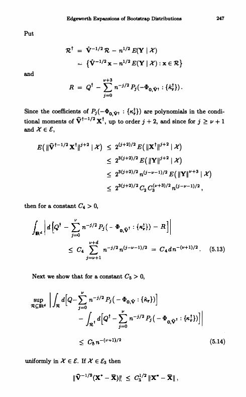
Put
and
Edgeworth Expansions of Bootstrap Distributions
'Rt = y-l/2 'R - n1/2 E{Y I X)
{y-l/2 X - n1/2 E(Y I X) : X E 'R}
11+3 R = Qt - L n-jf2 �(-�o;vt : {kt}) .
j=O
247
Since the coefficients of Pj { -�o vt : {Kt}) are polynomials in the condi
tional moments of "t-1/2 Xt , u� to order j + 2, and since for j � 1/ + 1 and X E £,
E( l I"t- 1/2 xt 1 IJ+2 I X) < 2(j+2)/2 E{ I Ixt 1 IJ+2 I X) < 23(J+2)/2 E( IIY IIJ+2 I X) � 23(j+2)/2 n(j-II- l)/2 E( I IYII',+3 I X) � 23(J+2)/2 C
2 C�"+3)/2 n(j-lI-l)/2 ,
then for a constant C4, > 0,
lI+d � C4, E n-j/2 n(j-II-l)/2 = C4, dn-(v+l)/2 . (5. 13)
j=v+l
Next we show that for a constant Cs > 0,
1lS��" 1 1 d [Q-� n-j/2 Pj { - �o.v : {kr})]
- 1, d [Qt - � n-jf2 Pj { - �o.vt : {Itt})] I (5. 14)
uniformly in X E £. If X E £3 then

5. DetaIJa of Mathematical Rigour
and so by Markov's inequality
p{ II'V-1/2 (X· - X) II >nl/2 I X} � C�V+3)/2 n-{v+3)/2 E( I IX· - Xllv+3 I X) � C2 C�V+3)/2 n-(v+3)/2 .
Therefore, with Cs = C2 C�V+3)/2 ,
whence sup IQ(R.) - Qt(R.t ) 1 � C6 n-(II+l)/2 . (5.15)
'R.�IR. Moreover, if j � 11 + 2 then any conditional jth moment of V-1/2 {X· - X) differs from its counterpart for xt by O(n-<v+l)/2 ) , as follows from the inequalities
E{ I Ixt - V-1/2 (X· - X) I I; I X} � 21 E [ I IV-1/2{X· - X) lIi I{ IIV-1/2 (X· - X) II > n1/2 } I X] $ V n{j-(2v+3)}/2 E{ I IV-1/2 (X· - X) 1 1211+3 I X} � 2"+2 C2 C�211+3)/2 n -(11+1)/2 .
Therefore, for a. constant C7 > 0 not depending on n,
sup I r d [� n-j/2 P;(-� . : {kr})] 'R.CR J.,. � o,v - 'R. 3=0
- [ d [t n-j/2 Pj (-�o;vt : {it!})] I J'R.t j=O
uniformly in X E e. The claimed result (5. 14) follows from this inequality and (5. 15).
Combining (5. 13) and (5. 14) and taking C8 = C4 d+ C5 , we deduce that
(5. 16)

Edgeworth Exp&IIIIions of Bootstrap Distributions 249
Next we develop an upper bound to I i'R.t dRI , by smoothing the mea.sure R. Write B(x, r) for the closed sphere in IRd centred at x and with radius r. Let L be a probability density on Rd with support confined to B(O, 1) and Fourier transform (Le. , characteristic function)
satisfying
IDr L(t) 1 :5 09 exp( -UtU 1/2) ,
for all t E Rd and all d-vectors r = (r(1) , . . . , r(d» )T with nonnegative integer components such that
d Ir l = L r(j) :5 d + 1 . j=1
Here Dr denotes the differential operator
r d ( lJ ) r(j) D = II (j) j=1 a t
Define L.s (x) = 6-d L(6-1 x) for 0 < 6 :5 1 , and let L.s (t) = L(6t) be the corresponding Fourier transform. There exists a constant OlD > 0 such that for any function 9 : IRd -+ JR with Fourier transform g,
r Ig(x) 1 dx :5 OlD max J. IDr g(t ) 1 dt . (5.17) JIR4 r: lr l=O,d+l R4
Take 9 to be the density of the measure G defined by
G('R) = r L.s(Y) dyl dR . JlRd 'R.-y
Then g = L6 p, where p is the Fourier-Stieltjes transform of the distribution function corresponding to the measure R, and so
r Ig(x) l dx :5 OlD max r IDr{L.s (t) p(tH l dt JlRd Irl=O, d+l Jm.d
where the inequality 0 :5 r :5 8 is to be interpreted elementwise. Write lJ'R for the boundary of 'R, and (8'R.) £ for the set of all points in IR d distant no more than E from {JR.. Then, since L vanishes outside BCO, 1) , we have for

250 5. Details of Mathematical Rigour
any 'R. � Rd,
1 1 dR / $ hv Ig(x) 1 dx
lI+d + L n-;/2 f Ipj ( - tPo;vt : {ki}) {x) I dx , (5. 19) j=O J(8'R.)2'
where 9 is lIB defined just above. Replacing 'R. by 'R.t and combining (5. 18) and (5. 19) we deduce that
I f dR I $ C11 max 1. IDr L6 (t) I IDs-r p(t) 1 dt J�t O�r�s Rd 181�d+1
lI+d + L n-j/2 f Ipj ( - tPo;vt : {kt}) (x) I dx . (5.20) j=O J(8'R.t)21
To simplify the first term on the right-hand side of (5.20) we need a standard result on Taylor expansion of characteristic functions, which we state here without proof. The lemma is a special CIlBe of Theorem 9.9 of Bhattacharya and Rao (1976, p. 77) and of Lemma 8 of Sazanov (1981 , p. 55) . It applies to an expansion of the characteristic function of a general random variable, which for simplicity we write as X.
LEMMA 5 . 1 . Let X denote the characteristic function of a d-variate ran
dom variable X with zero mean, nonsingular variance matrix V, and cu
mulant sequence {It II } . Assume that EIiXlim < 00 for some integer m � 3. Let C > 0 be a constant such that tT V2 t $ C implies Ix(t) - 1 1 $ � . There exist absolute constants C12 and C13, depending only on d an d m,
such that for all vectors r = (r(I) , . . . , r(d» T with nonnegative integer com
ponents satisfying L Ir(j) I $ m,
/Dr [x(n-1/2 V-1/2 t)n - exp ( - � I I t 1 l2) I: n-j/2 Pj (iV-1/2 : {It II })] / j=O $ C12 EI IV-1/2 Xllm n-(m-2)/2
x ( I It l lm- lrl + I It I l3(m-2l+lrl ) exp (- t I It 1 l 2) (5.21)
uniformly in / It I I $ n1/2 min {Cl/2 , CI3 (EIIV-l/2 Xllm)-I/(m-2) } .
In the lemma, replace X by xt (conditional on X) and take m = max(v + 3, d + 1 ) .
Then V changes to Vt and X(t) is replaced by xt (t) = E{ exp(itT Xt) I X} .

Edgeworth Expansions of Bootstrap Distributions 251
If X E &, then
1 1 - Xt (t) 1 :5 tT yt t :5 2e t and
..... t2 whence t T V t :5 te implies 1 1 - X t (t) I :5 ! . Therefore, we may take C = l� in the lemma. Furthermore, if X E &2 n &3 n &4 ,
E( l Iyt-1/2 Xt l lm I X) :5 2m/2 E( l lxt l lm I X) < 23m/2 E( I IYllm I X)
< �m/2 C;/2 E ( I IX· _ Xllm I X)
:5 �m/2 C;/2 C2 = Cu , say. Defining Cus = min ( 1 , Cl3 Cu.l/(m-2» , we deduce from (5 .21) that
if X E & and I r l :5 m,
IDr p(t) I :5 Cl2 Cl4 n-(m-2)/2 ( I It l lm- 1rl + I I t I 1 3(m-2)+ lrl ) exp ( - 1 1 I t I 1 2) uniformly in I I t l l :5 C1S n1/2 . Since IDr L.s (t) I :5 C9 then
max r IDr l.s (t) I IDs-r p(t) 1 dt :5 Cl6 n-(Ii+1)/2 , (5.22) O$r$a ill t ll $C n1/2 Is l $d+1 18
where
Cl6 = C9 Cl2 Cl, max r ( i l t l lm-r + I l t I l 3(m-2)+r) exp (- 1 I lt I 1 2) dt . O$r$m ilRd
Next we develop a formula analogous to (5.22) , in which the integral over I I t l l :5 ClS nl/2 on the left-hand side is replaced by an integral over
I I t l l > ClS nl/2 . Let 1/J denote the characteristic function corresponding to
the probability measure Q t , and observe that
£1+3 p(t) = 1/J (t) - exp ( - ! I I t 1 l 2) L n-j/2 Pj (iyt-l/2 t : {itt }) .
j=O If X E & then for a constant C17 > 0,
Ir��l IDr [ exp ( - ! I l t 1 1 2 ) � n-j/2 Pj (iVt-1/2 t : {R:t}) ] I :5 C17 exp ( - 1 I lt I 1 2)
uniformly in t, and so
max r IDr l.s(t) I IDs-r {p(t) - 1/J(t)} 1 dt O$r$., 1.I $d+1 illtl l >cu n1/2
(5.23)

252 5. Details of Mathematical Rigour
The lemma below provides an upper bound to
Let X* (t) = E{ exp(ie X·) I X} denote the empirical characteristic
function of the sample, and note that X = E(X·) .
LEMMA 5 .2 . Assume that the distribution of X satisfies Cramer's condition. Then there exist positive constants CI9 E (0, 1) , C20, C21 , and C22 such that whenever X E £, 0 < 6 < 1, n > 2(d+1) , and m E [1 , n-(d+l)] ,
a.s � C20 nd+1 J [C�9 + {C21 Ix· (n-I/2 t) - x(n-1/2 t) l }m]
(5 .24)
A proof will be given in step (iv) . In the meantime, take 6 = n-u , where u is yet to be chosen. Since
uniformly in t, then by Markov's inequality, the set
£5 = {X : J Ix* (n-(l/2)+u t) - x(n-(1/2)+u t) lm exp( -C22 1 It I l 1/2) dt
� n-d(u+1)-(v+3)/2 }
satisfies P(t5) = O(n-�) , provided m (fixed, not depending on n) is chosen sufficiently large. Henceforth we shall assume that X E £' = £ n £5 ; note that by (5. 11 ) ,
pet) = O(n-�) . For such an X we may deduce from (5.24) that
Combining this result with (5.20) and (5.22) we conclude that with
6 = n-u,
where
I L t dR I � Cn (C16 + C24) n -(1'+1)/2 + b6 , (5.25)
v+d 1 b6 = L n-j/2 I pj ( - ¢>o;vt : {kt J) (x) l tlx
j=O (8Rt)21
uniformly in X E £' and 1l � Rd.

Edgeworth Expansions of Bootlltrap Distributions 253
The remainder of our proof is directed at obtaining an upper bound for b6 , uniformly in sets 'R of the form (5. 12) . Note that the function
equals a polynomial of degree 3j multiplied by exp (- � X T yt-1 x) . The coefficients in the polynomial, albeit random, are bounded uniformly in X E £, and so
b6 $ C25 r (1 + I IxIl3(1I+d») exp ( - � xT Vt-1 x) dx . J(lYR,t)26 / � 1/2 -
Define a = -n1 2 Y E(Y I X), recall that S denotes the complement of a set S, and observe that if X E £,
{y1/2 x : x E (8'R.t)26 }
= {y1/2 x : x E 'R.t and B(x, U) n ('Rtt 1= 0 , or x E ('Rt)- and B(x, 26) n 'R.t 1= 0}
{ � 1/2 � 1/2 -X : x E 'R. + a and [V B(Y- x, 26)] n ('R. + a) 1= 0 , or x E ('R + af and [Vl/2 B(y- 1/2 x, 26)] n ('R. + a) 1= 0}
� {8('R + an 'I ,
where 11 = C26 o. Furthermore,
I I a l l = n1/2 1 IE [(X· - X) I { I IY-1/2 (X· - X) II > n1/2 } I X] I I
$ n1/2 Ci/2 E [ I IY-1/2 (X· - X) II I{ I IY-l/2 (X· - X) I I >n1/2 } I X]
$ C;/2 E{ I IY-l/2 (X· - X) 1I2 I X} = Ci/2 .
Therefore,
Assume 'R. = 'R(t) has the form (5. 12), and note that we may write
where
n1/2 A(X + n-1/2 x) = A1 (x) + A2 (x) , (5.27)

254 5. Details of Mathematical Rigour
and
IA2 (x) 1 � C29 n-(I'+2)/2 (log n)"+3 , the latter uniformly in X E £ and I Ixll � log n. All the derivatives A(i" . . . ,ij ) (X), 1 � j � 1/ + 3, are bounded uniformly in X E £1 ' Take u = i (1/ + 2), and remember that "I = C26 n-u• In consequence of (5.27) , and provided X E £,
{8R.(t)}" = {Xl E IRd : for some X2 E IRd, n1/2 A(X + n-I/2 X2) = t , and I lxI - x2 11 � Tf}
� 'Rl (t) U {B(O, log n)f ,
where
'Rl (t) = {x E IRd : I Ix ll � log n and AI (X) E [t - C29 n-(I'+2)/2 (log n)"+3 ,
t + C29 n-(I'+2)/2 (log n),,+3] } . It follows from this relation and the lemma below that for X E £,
LEMMA 5 .3 . Let U have the d-variate Normal N(O, I) distribution, let /3, b > 0, and let
rex) = L Co XCi) + n-1/2 L L Coti2 xCi, ) x(i2) + . . . i il '2
+ n-(v+1)/2 '" . . . '" £" • X(i" X(iu+2 ) � � '""1 1 . . . 1,,+2 • • • il i"+2
be a polynomial in X and n-1/2 whose coefficients Co, Ci,i2 ' • . . , eo, . . . iu+2 satisfy
. m8:X (ICi, I ICi,i2 1 , . . · , ICo, . . . iU+2 1 ) � b , I I , , , ' t' ... +2
and for some i (1 � i � d), leo l > i . There exists C > 0, depending only on (3, b, and d, such that
sup p{ I IUI I � b log n and r(U) E It - n-�, t + n-�l } � C n-fJ • -oo<t<oc
Lemma 5.3 is trivial if d = 1 , and may be proved by induction for general d.

Edgeworth Expansions of Bootstrap Distributions
Results (5.26) and (5.28) together imply that
b.s $ C27 C30 n-(V+1)/2
255
uniformly in sets 1l = 1l(t) of the form (5.12) and samples X E E. Combining this with (5. 16) and (5.25) we conclude that for X E E',
sup I f d [Q - t n-j/2 Pj (-410;v : {�r})] 1 $ C31 n-(v+1)/2 , -oo<t<oo J'R.(t) j=O
where C31 = Cs + C11 (C16 + C24) + C27 C30 • Equivalently,
-.:�r<oo I P{nl/2 A(X*) $ t I X} -� n-j/2 Pj { - 410,v : {�r}) {1l(t)} 1
$ C3l n-(v+1)/2 uniformly in X E E'.
(5.29)
Bearing in mind the definition of Pj given in part (i) of this proof, it is straightforward to Taylor expand the series in Pj in (5.29) , obtaining
sup I p{ n1/2 A(X* ) $ x I X} - 41(t) - t n-j/2 1'j (x) t!J(X) I -00<.,<00 ;=0 < C n-(v+1)/2 - 32 (5.30)
uniformly in X E E, where rj is a polynomial of degree 3j - 1, odd or even for even or odd j, and with coefficients depending on the cumulant sequence {�r} up to order j + 2. In order to establish result (5.7) it remains only to prove that 1'; = Pj or q; , depending on the definition taken for A.
(iii) Identifying the Expansion
Let the function A be defined by (5.1) or (5.2) , and let rj denote the version of l' j when the cumulant sequence {�r} is replaced by {Kr } . A substantially simpler version of the argument leading to (5.30) shows that under identical regularity conditions,
-':��< oo Ip{n1/2 A(X) $ x} - 41(x) - t n-j/2 rj (x) t!J(X) I (5.31)
Therefore, it suffices to prove that rj = Pj or qj , depending on the circumstance. This is simply a matter of equating the coefficients in rj with those in Pj or qj , which depend only on a finite number of population moments or cumulants. All possible sets of values of these quantities are assumed

256 5. Details of Mathematical Rigour
in the case where the distribution of X is essentially bounded (i.e. , for some C > 0, P(I IXI I $ C) = 1) , and so we may suppose without loss of generality that X enjoys this property.
Let 1fj = Pj if A(x) = {g(x) - g(p)}/h(p)
and
1fj = qj if A(x) = {g(x) - g(pH/h(x) .
We must prove that T j = 7r j . If the distribution of X is essentially bounded then we may Taylor expand Sn = n1/2 A(X) , as at (2.28) and (2.29) , obtaining
where d d d
Sn,lI+1 = L <Ii Z(i) + n-1/2 ! L L at. i2 Z(i1 ) Z(i2) + . . . i=1 i1 =1 i, = 1
d d -11/2 1 '"' '"' a . . Z(il ) Z(i"+l) + n (lI + l)! L ' " L · 1 · · ··"+1 . . . ,
i 1 = 1 i,,+1=1
Ci1 . . . i.1 (lJi /8x(i, ) . . . 8x(o; » A(x) lx=,. ,
Z = n1/2 (X - p) ,
and for each E, >. > 0,
p( IR.-I > n-(II+1)/2+f ) = O(n-.A) .
Recall from Theorems 2.1 and 2.2 in Section 2.4 that for 1 $ j $ II, 7rj is defined uniquely by the property that for each 1 $ k $ j + 2, the kth moment of Sn.,I1+1 equals
1: x/c d{ �(x) + t n-i/2 'Trj(X) 4>(x) } + o(n-II/2) .
(Equivalently, the definitions can be given in terms of cumulants; note the expressions for cumuiants in terms of moments at (2.6) .) Therefore, it suffices to prove that for k � 1,
E(S!,II+1) = 1: x/c d{ �(x)+ t n-j/2 Tj (X) 4>(x) } + o(n-II/2) . (5.32)
Observe from (5.31) that for 0 < E $ ! ,
sup I p(S" $ x ± n-(1I/2)-E) - P(S" $ x) I = O(n-(1I/2)-f) . -00<"'<00

Edgeworth ExpansiODB of Bootstrap DiBtributioDB 257
Therefore,
sup I peS,. 5 :r:) - P(S,.,II+! 5 :r:) 1 - 00 < 2: < 00
5 sup max I p(S,. 5 :r: ± n-(1I/2)-E ) - pes,. 5 :r:) 1 -00<2:<00 +,-
+ P(lR,.1 > n-(1I/2)-E)
= O(n-(II/2)-E ) .
This result and (5.31) imply that for all 0 < E 5 i ,
II sup I P(S,.,II+1 5 :r:) - �(:r:) - E n-;/2 r; (:r:) q,(:r:) I
-00<2:<00 ;=1
= O(n-(1I/2)-E ) .
Given c > 0, take 6 = f/2c, and note from (5.33) that
II sup (1 + I:r:n Ip(S,.,II+! 5 :r:) - �(:r:) - E n-;/2 r; (:r:) q,(:r:) I
12: 1 �"· ;=1
By Markov's inequality we have for each 6, � > 0,
p( lS,.,II+! 1 > noS) = O(n-") .
(5.33)
(5.34)
(Here we have again used the fact that X is essentially bounded.) Therefore, the supremum in (5.34) may be taken over all :r:: for all c > 0,
II sup (1 + 1:r: 1" ) Ip(S".II+! 5 :r:) - �(:r:) - E n-;J2 r; (:r:) q,(:r:) I
- 00 <2:< 00 ;=1
Hence, integrating by parts,
5 k L: 1:r: 1 "'-1 Ip(S,.,II+! 5 :r:) - �(:r:) - � n-;/2 r; (:r:) q,(:r:) I d:r:
= o(n-II/2} .
This establishes (5.32) and completes the proof of the theorem..
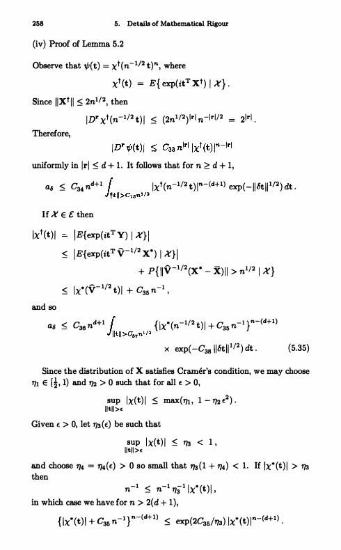
258 5. Details of Mathematical Rigour
(iv) Proof of Lemma 5.2
Observe that 1/!{t) = xt(n-l/2 t)n, where
xt (t) = E{ exp(itT xt) I X} .
Since I Ixt l l � 2nl/2, then
IU xt (n-l/2 t) 1 � (2nl/2) /r / n- /r //2 = 2Ir / .
Therefore,
uniformly in Ir l � d + 1 . It follows that for n � d + 1,
a6 � C34 nd+l r Ixt (n-l/2 t) ln-{d+l) exp( - 1I 6t l l l/2 ) dt . J"t ll >ClSn1n If X E £ then
Ixt (t) 1 IE{exp(itT y) I X} I
and so
� IE{exp(itT Y-l/2 x· ) I Xl i + P{ IIY-l/2 (X· _ X) I I > n1/2 I X}
� IX* (y-l/2 t) 1 + C35 n-l ,
a6 � C36 nd+l r { lx* (n-1/2 t) 1 + C35 n-l r-(d+l) Jlltl l >cS7nl/2
x exp( -C3s I 16t I l 1/2 ) dt . (5.35)
Since the distribution of X satisfies Cramer's condition, we may choose 'TIl E [� , 1) and 1/2 > 0 such that for all f > 0,
sup Ix(t) 1 � max(7'/b 1 - 7'/2 (2 ) . I Itl l >· Given t > 0, let 7'/3 (f) be such that
sup I x(t) 1 � 7'/3 < 1 , / ltl l >·
and choose 114 = 1/4(f) > 0 so small that 7'/3 (1 + 114) < 1 . If Ix* (t) 1 > 'TI3 then
n-1 � n-l TJi1 Ix· (t ) l , in which case we have for n > 2(d + 1) ,
{ lx* (t) 1 + C35 n-1 } n-{d+l) � exp(2C35/'73) Ix* (t) ln-(d+l) .

Edgeworth Expansions of Coverage Probability
H Ix* (t) 1 � TJ3 then
{ lx* (t) 1 + C35 n-I r-(d+l) � exp(2C35/TJ3) '7;-(d+l) .
H Ix* (t) - x(t) 1 � TJ4 Ix(t) 1 and l it I I > f then
Ix* (t) 1 � 1J3(1 + TJ4) '
H Ix* (t) - x(t ) 1 > TJ4 Ix(t) 1 then for any m E [1 , n - (d + 1)] ,
Ix* (t) l n-(d+l) � { (1 + TJi1 ) lx* (t) - x(t) l }m .
259
Combining these estimates we deduce that for any f > 0 we have for all l i t I I > e,
{ lx* (t) 1 + C35 n-I r-(d+l) � exp(2C35/TJ3) [{ TJ3 (1 + TJ4) }n-(d+l)
.., - 1 l'f 1'In _ 1 ,/4 - :4 '/10 - 2 '
if 1/2 1= � , and
+ { (I + TJ(1 ) Ix* (t) - x(t) l }m] . (5.36)
TJ3 max U , sup Ix(t) l } , I It l l >·
C19 = max U (1 + '71 ) ' 1 - ! TJ2 e2 } � TJ3 (1 + TJ4) ' Substituting (5.36) into (5.35) , and defining C20 = C36 exp(2Ca5ITJa) and
C21 = 1 + TJi1 , we obtain (5 .24) . This completes the proof of Lemma 5.2.
5.3 Edgeworth Expansions of Coverage
Probability
Our aim in this section is to provide a rigorous justification of the results developed in Section 3.5, particularly Proposition 3. 1 . From that flow most of our conclusions about the manner in which various orders of correctness influence the coverage properties of confidence intervals. We shall develop formulae for coverage error up to terms of size n -1 , with a remainder of o( n -I ) . Higher-order expansions, useful for describing coverage properties of symmetric intervals or iterated bootstrap intervals (see Sections 3.6 and 3. 1 1 ) , may be established rigorously by similar means. Throughout our development we assume the "smooth function model" described in

260 5. Details of Mathematical Rigour
Section 2.4 and subsection 5.2.1 . In particular, 80 = g(p), 8 = g(X), and (; = heX) , where g, h are smooth functions from Ref to R, X denotes the mean of a d-variate random sample X = {Xl , ' " , X,,}, and I' = E(X) is the population mean.
To begin, we recall the coverage problem introduced in Section 3.5. Let
denote a one-sided confidence interval, where z'" = w-1 (a) and
A -1/2 A ( ) + -1 A ( ) + Co. = n 81 Z'" n 82 Z'" • • •
for polynomials 8; . We wish to develop an Edgeworth expansion of the probability P(80 E II) ' In many cases of practical interest, 8; is obtained by substituting sample moments for population moments in a polynomial 8; , which is of degree j + 1 and is odd or even according to whether j is even or odd. (This follows from properties of Cornish-Fisher expansions, described in Sections 2.5 and 3.3.) We claim that under moment conditions on X, there exist random variables MI, M2 that are linear combinations of sample moments of the form
" d M = n-1 E II (Xl;» /J ,
i=l j=l
and fixed constants b1 ' � ' such that for f, 8 > 0 sufficiently small,
P [ "_.�:�t,,_. lc,,, - {n-1/2 81 (z",) + n-1 82 (z", ) }
- n-1/2 {b1 (M1 - EM1) + � Z!(M2 - EM2) } I > n-1-6]
(5.38)
= o(n-1 ) . (5.39)
(In (5.38) , ll o ' " , ld denote nonnegative integers.) To appreciate why, observe that it is typically the case that for some
f., 8 > 0,
For example, if I1 is a percentile or percentile-t confidence interval then � = -U1-", - Z'" or � = -V1-", - z"" respectively, and then (5.40) follows immediately from Theorem 5.2. (See subsection 3.5.2 for discussion of forms that � can take.) IT M is given by (5.38) then for any specified

Edgeworth Expansions of Coverage Probability 261
1/ > 0, it may be proved by Markov's inequality that under sufficiently stringent moment conditions on X,
The same result holds if M is replaced by the linear combination Mi. Furthermore, since 81 is an even polynomial of degree 2,
and
where the tli 'S are constants, jJ.i is a sample estimate of a population moment J1-i, and tli({l.i - J1-i) = bi(Mi - EMi) + Op(n-I) , for approximate choices of the constant bi and the linear combination Mi of m� menta. Arguing thus, and noting that I z .. 1 � CI (log n) I/2 uniformly in
n-e � Q � 1 - n-' , we may prove that if E(I IXII ' ) < 00 for sufficiently large 1 then there exist M I , M2, constants bl , b2 , and f, 6 > 0, such that
n-c < .. < I -n-· p{ sup I S I (Za) - 81 (Za ) - bl (MI - EMI )
- -- � Z;(M2 - EM2 ) 1 > n-(1/2)-26} = o(n-l ) , (5.41 )
The desired result (5.39) follows on combining (5.40)-(5.42) .
We are now in a position to state and prove rigorously a version of Proposition 3.1 . Let II denote the confidence interval defined in (5.37). Put gj (x) = (8/8x(j» g(x), and observe that if M1 , M'J are linear combinations of sample moments of the form (5.38) then for constants CI , C2 not depending on n,
Define
i = 1, 2 .
aa = 0'-1 (bi Cl + b'J C'J z;) , (5.43)
where bi t � are as in (5.39) . If any of the components comprising the linear combination Ml or M2 is not an element of X, it may be adjoined by lengthening each data vector so that the new vectors include the appr� priate products of earlier terms. We shall assume that this lengthening has already been carried out, in which case each Mi is a linear combination of elements of X. Then we have the following version of Proposition 3. 1 .

262 5. Details of Mathematical Rigour
THEOREM 5.3 . Assume that 9 and h each have four bounded derivatives in a neighbourhood of p, that E(IIXII ' ) < 00 for sufficiently large l, that Cramer's condition (5.5) holds, that Co admits the approximation (5.39) for polynomials 81 and 82 , and that the distribution ofnl/2(8 - (Jo)/fJ admits the Edgeworth expansion
p{ nl/2 (8 - (Jo)/fJ :5 z}
= �(z) + n-I/2 ql (Z) 4>{z) + n-l q2 (Z) 4>(z) + o(n-I ) (5.44)
for polynomials ql and Q2 . Then for the same t appearing in (5.39) , and with all< defined by (5.43) ,
n_.<:�tn_. lp{(Jo E Il (a)} - a - - - n-l/2 rl (Za) 4>(za) - n- 1 r2 (Za ) 4>{Zo) 1 = o(n-l ) , (5.45)
where
and
r2 (Zo ) = Q2 (Zo) + 82 (Za) - i Zo 81 (Zo)2
+ 8l (Zo) {Za Ql (Zo) - Q� (zo) } - ao zo .
Existence of the expansion (5.44) is not really an 888umption, since it is guaranteed to hold uniformly in z under the other conditions of Theorem 5.3; see Theorem 2.2. Our formula for aa is equivalent to that given in (3.35) in Chapter 3, the only difference being that in (5.43) we have spelled out the way in which it depends on Zo and the constants b,, , CA: . Thus, (5.45) implies the expansion (3.40) of Proposition 3.1 , up to a remainder of o(n-I ) .
We do not specify the value of l in the theorem since our proof makes no attempt to be economical in terms of moment conditions.
It is not possible, in general, to extend the range of a in (5.45) from n-< :5 a :5 I - n-' to 0 < a < 1 . This follows from properties noted earlier
in connection with confidence intervals constructed by explicit skewness correction; see Section 3.8. In particular, there exist examples where all the conditions in Theorem 5.3 are satisfied but, owing to the fact that Zo + Co is not monotone increasing in a,
lim sup P{(Jo E Il (a)} of!
is bounded below 1 as n -+ 00. The interval I discussed in the second-last paragraph of Section 3.8, and also the accelerated bias-corrected interval (-00, YABC, o) introduced in subsection 3.10.3, can have this problem.

Edgeworth Expansions of Coverage Probability 263
However, if %01 + COl is monotone in a, and if (5.45) holds for some f > 1 , then we may replace the range n-E $ a $ 1 - n-' by 0 < a < 1. To
appreciate why, note that if (3 = n-' = o(n-l ) then
sup I P{90 E II (a)} - a - n-I/2 TI (Za) t/>(za) - n-l T2 (Za) t/>(za) I O<a�.B
= sup P{90 E II (a)} + o(n-l ) O<a�.B
the last identity following from (5.45); and similarly,
sup I P{90 E II {a)} - a l-.B�a<l
- n-1/2 rl (Za ) t/>(za ) - n-1 r2 {Za ) t/>{za) I = o{n- 1 ) .
In specific cases, such as that of the percentile method (where c.. = -U1-a - za) , or the "other percentile method" (c.. = ua - %01 ) ' or percentile-t (c.. = -V1-a' - za), or bias correction, it is not difficult to establish (5.39) for f > 1 , assuming sufficiently many moments of the distribution of X. In those instances, (5.45) holds uniformly in 0 < a < 1 .
We conclude this section with a proof of Theorem 5.3, for which the
following lemma is particularly helpful. Write V for the variance matrix of X, let {ltr} denote the multivariate cumulant sequence of X, and let
Pj {-�o,v : {ltr}) be the signed measure with density Pj {-t/>o,v : {ltr}) ; see part (i) of subsection 5.2.3 for more details. Write (8'R)" for the set of points distant no more than f from the boundary 8'R of 'Ii.
LEMMA 5 .4 . If E( I IX I I "+2 ) < 00 for an integer v � 0, and if Cramer's condition (5.5) bolds, then
II
P{nl/2 {X - p) E 'Ii} = E n-j/2 Pj ( - �o,v : {ltr}) {'Ii) + o(n-II/2 ) j=O
uniformly in any class R of sets 'Ii � IRd satisfying
as 1'/ ! o.
sup [ exp ( - ! I Ix 1 l 2 ) dx = 0{1'/) {5.46} 'R.ER J(8'R.)"
This result is almost the simplest form of Edgeworth expansion for a sum of independent random vectors; see Bhattacharya and Rao (1976, p. 215) .

264 5. Details of Mathematical Rigour
Since Mi is a linear combination of elements of X then we may write
Mi = V[ X for fixed vectors Vi , i = 1 , 2. Let 6 be as in (5.39), and define
p(a) = P{80 e II (a)} ,
U = nl/2 (O - (0)&-1 + n-1/2 { b1 (Ml - EMd + � Z�(M2 - EM2)} ,
A(x) {g(x) - g(lJ)} h(x)-l + n-1 {b1vI (x - lJ) + � z!vr(x - IJ) } ,
y± = -{ za + n-1/2 81 (Za) + n-1 82 (Za) } ± n-1-S ,
'R.± = 'R.±(a, n) = {x E Rd : nl/2 A(IJ + n-1/2 x» y± }
and
p± = P(U > y±) = P{nl/2 (X - IJ) E 'R.± } . (5.47)
In view of (5 .39),
(5.48)
uniformly in n-' S; a S; 1 - n-· . It is readily shown by Taylor expanding the function A about IJ that for sufficiently large no, the class of sets
R = {'R.±(a, n) : n � no, n-· S; a S; 1 - n-· }
has property (5.46) . Hence by Lemma 5.4 and formula (5.47) ,
II p± (a) = L: n-j/2 Pj (-�o.v : {�}) ('R±) + o(n-I) (5.49)
j=O
uniformly in n-· S; a S; 1 - n-·. Bearing in mind the definition of Pj given in part (i) of subsection 5.2.3,
we may Taylor expand the series in Pj in (5.49) to obtain
uniformly in n-' S; a S; 1 - n-·, where rl and r2 are polynomials. This brings us to a version of (5.31) in the proof of Theorem 5. 1 , after which point it remains only to identify the polynomials rl and 82' That part of the present proof may be conducted along the same lines as part (iii) of the proof of Theorem 5.1, showing that rl and T2 are determined by the cumulant argument used in subsection 3.5.2 to prove Proposition 3.1. Theorem 5.3 now follows from (5.48) and (5.50) .

Linear Regre&llion 265
5.4 Linear Regression
We discussed the case of simple linear regression in subsections 4.3.3 and 4.3.4 of Chapter 4, and showed that in several key respects it is different from the more traditional circumstances encountered in Chapter 3. In particular, a percentile-t confidence interval for the slope parameter has coverage error O(n-2) , rather than O(n-1 ) . However, the method of proof of results such as this is very similar to that in the traditional case (see Sections 5.2 and 5.3) , the only important difference being that we now work with weighted sums of independent and identically distributed random variables rather than with unweighted sums. In the present section we outline the necessary changes to proofs, using the case of slope estimation as an example.
We begin by recalling the basic ingredients of simple linear regression. The simple linear regression model is
where c, d, Xi , Yi , E, are scalars, c and d are unknown constants representing intercept and slope respectively, the Ei 'S are independent and identically distributed random variables with zero mean and variance 0-2 , and the Xi 'S
are given design points. The usual least-squares estimates of d and 0-2 are
n d = 0-;2 n-1 L: (Xi - x) (Yi - Y) ,
i=1 where
n o-� = n-1 L (Xi - x)2 ,
i= 1
n &2 = n-1 L f� ,
i=1
Yi - Y - (xi - x) d .
Since d has mean d and variance n-1 0-;2 0-2 then inference about d would typically be based on the statistic T = n1/2 (d- d) 0-.,/&, whose distribution may be estimated by the bootstrap, as follows.
Let X· = {Et , . . . , E�} denote a resample drawn randomly, with replacement, from the collection X = {f 1 . . . . , En} , and put
yt = C + Xi d + < = Y + (Xi - X) d + E; ,
where c = Y - :i d. Define y* = n-1 :E yt ,
n d"* = 0-;2 n-1 E (Xi - X) (Yi* - y* ) ,
1=1

266 5. Details of Mathematical Rigour
The conditional distribution of T" = n1/2 (rj: - d) U.,/u" , given X, approximates the unconditional distribution of T.
To see how we might develop Edgeworth expansions of the distributions of T and T" , first define Vi = (Xi - x)/U."
Then
up> = �./u , U?) = Vi f.du , Ui(3) = f.� u-2 - 1 ,
( 1) " (2)' (3)" Ui = f.:Ju , U. = Vi f'.i/u , Ui = f'.;2 u-2 - 1 ,
(U�l) U�2) U.(3») T U.� = (U�1) ' U�2)' U�3)" ) T 1. " ' " , J l t l '
n U n-l L Vi = (U(1) , V(2) , V(3» )T ,
i=1 n
U" = n-1 L Vi· = (U(l) " , V(2)" , V(3) ' )T , i=1
T = n1/2 A(U) , T" = n1/2 A(U") .
This makes it clear that T and T" may be expressed as smooth functions of means of independent random variables. Therefore, we may use minor modifications of the methods employed to prove Theorems 2.2 and 5.1 to establish Edgeworth expansions. Indeed, if qj and qj , j � 1 , denote the polynomials introduced in subsection 4.3.3 of Chapter 4, then the following result may be proved.
THEOREM 5 .4 . Assume that E(/f /211+4) < 00 for an integer 1/ � 0, that Cramer's condition
lim sup /E{exp(it �) } / < 1 (5.51) I t l-oo
holds, and that {Xi } represents a sequence of independent realizations of 8. random variable X with E(/X/"+2) < 00 and var(X) > O. Then for a C18S8 of sequences {Xi } arising with probability one,
sup /P(T � W) - �(w) - t n-j/2 qj (W) rP(W) I -oo<w<oo j=l
(5.52)
as n --+ 00. If >. > 0 is given, and if the moment conditions on f'. and X are strengthened to E(k/21) < 00 and E(/X/I) < 00 for a suiliciently large

Linear Regression 267
l = l(A), then for a constant C > 0,
p{ _()()s�E<()() IPII(T* :5 w I X) - IP(w)
- L n-j/2 qj (w) 4>(w) I > cn-(II+l)/2 } = O(n-�) (5.53) as n -+ 00 . j=1
Taking A > 1 in (5.53) we may deduce from the Borel-Cantelli lemma that
-()()�E<()() Ip(T* :5 W I X) - IP(w) - � n-j/2 qj (w) 4>(W) I = o (n-(II+l)/2) (5.54)
with probability one. Result (5.54) is an explicit form of (4.29), under specified regularity conditions, and likewise (5.52) is an explicit form of (4.27) . Expansions of coverage probability. such as that in (4.41) . may be derived by doing no more than paralleling the arguments in Section 5.3.
We conclude by outlining the proof of Theorem 5.4. Let Vi denote the variance matrix and {/trt'} the cumulant sequence of Ui • and put
n -
- 1 '" V = n L..J Vi . i=1
n - -1 '" It.- = n L..J K.r,i •
i=1 Define the signed measure Pj( -IPo, V : {itr}) as in part (i) of subsection 5.2.3. The following analogue of Lemma 5.4 may be proved by an argument similar to that which produced Lemma 5.4.
LEMMA 5 .5 . Assume that E( lf I2I1H) < 00 for an integer 1/ � 0, that Cramer's condition (5.51) bolds, and that {Xi} represents a sequence of independent realizations of a random variable X with E( IXI"+2) < 00 and var(X) > O. Then for a class of sequences {Xi} arising with probability one,
II L n-j/2 Pj (-IPo,v : {itr}) (n) + o(n-II/2) (5.55) j=O
uniformly in any class R of sets 'R. � IR3 satisfying
as '1 1 0.
To prove (5.52). take
'R. = 'R.{n, z) = {y E m.d : n1/2 A{n-1/2 y) :5 z}

268 5. Details of Mathematical Rigour
in (5.55) , and Taylor expand
Pi(-�O,v : {;c,.}) (1l(n, x»
about
using techniques from part (iii) of subsection 5.2.3 to identify terms in the resulting expansion. The proof of (5.53) is very similar to that of Theorem 5. 1 in Section 5.2, with only minor modifications to take account of the fact that the random series involved are now weighted sums of independent and identically distributed random variables.
5.5 Nonparametric Density Estimation
5. 5. 1 Introduction
Let X = {Xl , ' " , Xn} denote a random sample from a population with density f. In Section 4.4 we developed Edgeworth expansions for the distribution of kernel-type nonparametric density estimators of f, in both the Studentized and non-Studentized cases. All the statistics involved may be represented very simply in terms of smooth functions of sums of independent and identically distributed random variables. For example, the Studentized estimator has the form
T = T(x) = {i(x) - E](x) } / { (nh)-l A(x) - n-l ](x)2 } 1/2 , (5.56)
where lex) = A(x), n
]j (x) = (nh)-l L K{(x - X.)/h}j , (5.57) i=1
and h denotes the bandwidth. Therefore, in principle, the techniques described earlier in this section go through with little change, and Edgeworth expansions may be developed for both T and its bootstrap approximant.
However, there is one technical difficulty, that of Cramer's condition. It is not immediately obvious that the random variable
Y = K{(x - X)/h}
will satisfy an appropriate version of Cramer's condition. Indeed, if K is the so-called uniform kernel,
K(y)
= { ! if Iyl � 1 ,
otherwise ,

Nonparametric Density Estimation 269
then Cramer's condition fails. This feature, and the fact that the orders of magnitude of terms in Edgeworth expansions for nonparametric density estimators are nonstandard, indicate that we should spend some time recounting rigorous theory for the expansions described in Section 4.4. The present section is devoted to that task. Subsection 5.5.2 states a variety of expansions from Section 4.4, under explicit regularity conditions, and subsections 5.5.3 and 5.5.4 provide proofs.
5. 5. 2 Main Results
We need the following notation from Section 4.4. Define ij and T as in (5.56) and (5.57) , and put
J1.j = J1.j (x) E{jj (x)} , Jl.ij = /1-ij (X) = h- 1 E( [K{(x - X)Jh} - EK{(x - X)/h}] i
x [K{ (x - X)/h}2 - EK{(x - X)/h}2]j) , S = S(x) = {j(x) - /1-1 (x) }/{(nh)-l /1-2 (x) - n-1 /1-1 (X)2} 1/2 ,
Pl (Y) -1 /1-203/2 /1-30 (y2 - 1) , P2(y) = - � /1-202 /1-40 y(y2 - 3) - � /1-2"03 /1-�0 (y4 - 10y2 + 15) ,
( ) 1 -3/2 1 -3/2 ( 3 ) ( 2 1) qlO Y = 2' /1-20 /1-11 - 6' /1-20 /1-30 - /1-11 Y - ,
q20 (y) = -/1-2"� /1-�0 y - (i /1-2"03 /1-�0 - f2 /1-2"02 /1-40)y(y2 - 3) - fa J1.2"� /1-�0 y(y4 - 10y2 + 15) ,
( ) -1/2 2 ql1 Y = -/1-1 /1-20 y . Let X* = {X; , . . . , X�} denote a resample drawn randomly, with replacement, from X, and define
n J;(x) = (nh)-l L K{(x - X;)/h}j ,
i=1 p.j p,j (x) = ij (x) ,
r = 1; ,
Aj = Aj(x) = h-1 E ( [K{(x - X*)/h} - E{K« x - X*)/h) I X}] ' x [K{{x - X*)/h} - E{K«x - X*)Jh) I X}] j I X) ,
S* S* (x) = {j* (x) - i(x)}/{ (nh)-1 i2 (X) - n-1 il (X)2}1/2 , T* T* (x) = {j* (x) - i(x)}/{(nh)-l i; (x) - n-1 i; (X)2 }1/2 .

270 5. Details of Mathematical Rigour
Let Pj &lld tlsj ha.ve the same definitions as Pj &lld qij , except that J.L1c &lld J.L1c1 are replaced by Pic &lld Plcl throughout.
The following regularity conditions are needed. The first guar&lltees a version of Cramer's condition, the second demands a minimal amount of smoothness of f, and the third asks that h satisfy the usual conditions for strong consistency of f:
K has compact support [a, b] j for some decompo-sition a = Yo < Yl < . . . < Yrn = b, K' exists and is bounded on each interval (Yj- l , Yj ) and is either strictly positive or strictly negative there; J K = 1 ;
f(y} = (d/dy) P(X � y) exists in a neighbourhood of x, is continuous at x, &lld satisfies f(x) > OJ
h = h(n) -+ O and nh/ log n -+ oo .
(5.58)
(5.59)
(5.60)
Condition (5.58) excludes the uniform kernel, which fails to satisfy our bivariate version of Cramer's condition (see Lemma 5.6 in subsection 5.5.3) , &lld that fact renders our proof inapplicable. However, an Edgeworth expansion for S(x) in the case of the uniform kernel may be derived by methods which are routine for lattice-valued random variables (e.g. , Gnedenko &lld Kolmogorov 1954, p. 212ff) , and extended to T(x) by noting that for the uniform kernel,
We are now in a position to state our main theorems about Edgeworth expansions, which make rigorous the work in subsections 4.4.3 and 4.4.4. The first expansion applies to the distributions of S and T, the second to the conditional distributions of S· &lld T· . We give here only the limited expansions used in Section 4.4. Longer exp&llsions are readily developed, using the general Theorem 5.8 proved in subsection 5.5.3.
THEOREM 5 .5 . Assume conditions (5.58)-{5.60) . Then 2
sup iP(S :5 y) - iIl(y) - � )nh)-j/2 pj (Y) <I>(Y) 1 - 00 <11<00 j=l
= O{ (nh}-3/2 } , {5.61}
2 sup Ip(T :5 Y) - �(Y) - L (nh)-j/2 qj (Y) <I>(Y} - (h/n}1/2 Q3(Y) <I>(Y) I
-00 <11<00 ;=1
= O{ (nh)-3/2 + n-l} . (5.62)
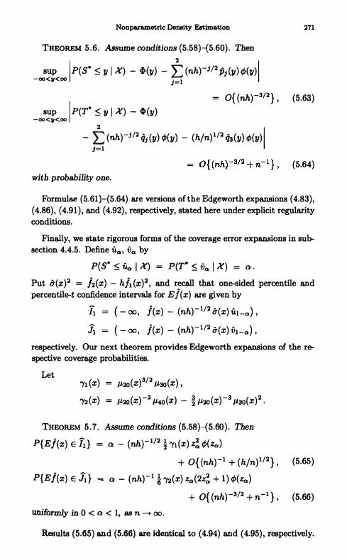
Nonparametric Density Estimation
THEOREM 5 .6 . Assume conditions (5.58)-{5.60) . Then
_oos�e<Jp(s· � y I X) - �(y) - t (nh)-j/2 13; (Y) 4>(Y) 1 = O{ (nh)-3/2 } ,
sup Ip(T· � Y I X) - �(y) -00<11<00 - t (nh)-j/2 tJj (Y) 4>(Y) - (h/n) 1/2 (ia(y) 4>(Y) 1
with probability one.
271
(5.63)
(5.64)
Formulae (5.61)-(5.64) are versions of the Edgeworth exp8Jl8ions (4.83) , (4.86) , (4.91 ) , and (4.92) , respectively, stated here under explicit regularity conditions.
Finally, we state rigorous forms of the coverage error exp8Jl8ions in subsection 4.4.5. Define Ua, Va by
peS· � Ua I X) = peT· � Va I X) = a .
Put U(X)2 = j2 (X) - hA (x)2 , and recall that one-sided percentile and percentile-t confidence intervals for Ej(x) are given by
It = ( - 00, j(x) - (nh)- 1/2 u(x) Ul-o) ,
h ( - 00, j(x) - (nh)- 1/2 u(x) Vl-o) ,
respectively. Our next theorem provides Edgeworth exp8Jl8ions of the respective coverage probabilities.
Let 'Yl (X) = J.£20(X)3/2 J.£30(X) ,
'Y2 (X) = J.£20 (x)-2 J.£40 (X) - $ J.£20 (X)-3 JL30(x)2 .
THEOREM 5 .7. Assume conditions (5.58)-(5.60) . Then
P{Ej(x) E It} = a - (nh)- 1/2 ! 'Yl (X) z� 4>(zQ)
+ O{ (nh)-l + (h/n?/2 } , (5.65)
P{Ej(x) E h } a - (nh)- l ! 'Y2(X) zQ(2z! + 1) 4>(zQ)
uniformly in 0 < a < 1, as n ---+ 00. + O{ (nh)-3/2 + n-1 } , (5.66)
Results (5.65) and (5.66) are identical to (4.94) and (4.95) , respectively.

272 5. Detaill of Mathematical Rlgour
5. 5. 9 Proof of Theorems 5. 5 and 5. 6
We begin by introducing essential notation. Let
Yr = K{(x - x)/hY - E[K{(x - x)/hYJ and write V = (vra ) for the 2 x 2 matrix with Vn = /-L20, V12 = /-LIb V22 = /-L02 . Put t = (tb t2)T and define the polynomial PjI.(tb t2 ) by the formal expansion
exp [U-2� (_V)k (k + 1)-1 {� ii (j!)- l Ui h-1 E(tlYI + t2Y2)i r+l] 00 i/2
= exp( - ! eVt) { I + E E ui vk P;k(t} , t2) } . ;=1 k=O Let Q;k be the signed measure whose Fourier-Stieltjes transform is exp(- ! tTVt) Pj1c (t) ,
r exp(itTy) dQ;k (Y) = exp(-! tTVt) Pjk(t) . JIll The density of Q;k may be written as p;k (Y) ,po,v (Y) , where P;k is a polynomial whose coefficients are rational polynomials in the moments }Jr., and
¢a,v is the bivariate normal N(O, V) density. Let �o,v denote the N(O, V) probability measure.
Let V, Q;k, P;k be the versions of V, Q;k , Pjk respectively, obtained on replacing /-Lra by ji,ra (for each r, s) wherever it appears in the respective formulae. Define
n Snr = (nh) -1/2 E [K{ (x - X;)/hY - EK{ (x - X;)/hY] , ;=1 n S�r = (nh) -1/2 E [K{ (x - Xj)/hY - hir(x)] ,
;=1
Write 8'R. for the boundary of a set 'R � JR2 and (trR.)< for the set of all points distant no more than E from 8'R.. We first prove a precursor to Theorems 5.5 and 5.6.
THEOREM 5.8. Assume the conditions of Theorem 5.5. Let R denote II class of Borel sets 'R � ]R2 that satisfy
sup [ exp ( - � I lxll 2) dx = O(E) 'RoEll J(lYR.)"

Nonparametric Density Estimation 273
as f ! O. Then for each integer v � 1 ,
��� IP(Sn E 'R) - �o,v('R) - t � (nh)-j/2hlc Qjlc ('R) I = O{ (nh)-(&I+l)/2} , (5.67)
I &I j� I sup P(S� E n I X) - �o.v('R) - L L (nh)-j/2hIcQjlc (n) �ER j=1 k=O
the latter result bolding with probability one.
Our proof of Theorem 5.8 is prefaced by three lemmas.
LEMMA 5.6. Under conditions (5.58) and (5.59) we have for each f > 0,
sup 1 100 exp{itl K(u) + it2 K2(u)}d,.F(x - hu) 1 � 1 - C(x, f)h
I td+lt2 1>< -00 for all sufIiciently smaJ1 h, where C(x, f) > O.
Proof·
Let a, b be as in condition (5.58) , and observe that
I(tl J t2)
= -I: exp{it1 K(u) + it2 K2(U)}d,. F(x - hu)
1 - h lb /(x - hu) du + h/(x) lb exp{itl K(u) + it2 K2(U)} du
+ h lb exp{itl K(u) + it2 K2 (u) } {/(x - hu) - /(x) } du .
We claim that the conditions imposed on K imply that for each
-00 < c < d < 00, and each
there exists f' > 0 such that

274 5. Details of Mathematical Rigour
Accepting this for the time being, take c = a and d = b, and choose h so small that
Then
i
b
I /(x - hu) - l(x) 1 du < (b - a)/(x) E' •
II(h , t2 ) 1 :$ 1 - h(b - a) I(x) (l - l) + h(b - a) I(x) (l - 3f') + h(b - a) l(x)E'
= 1 - h(b - a)/(x)l ,
which gives Lemma 5.6.
Finally we check (5.68). Observe that
ib
exp {it! K( u) + it2 K2( u) } du
m i
K(IIJ ) = L exp (it1 u + it2 u2) dK-l (U) ,
j=1 K(Yj _ , )
where K-l is interpreted in the obvious manner. Define
and note that
L(u) = d� K-l (u) = 1/K'{K-1 (u)} ,
I rK(Yj )
IL(u) 1 du l = Yj - Yj-l < 00 . J K(Yj - l l
Therefore L is integrable on the interval Ij = (aj , bj ) where endpoints are K(Yj ) and K(Yj- l ) . Result (4.68) will follow if we prove that for each E > 0 and each i ,
sup lib; eXP (it1 U + it2 u2) 1 < l i
bj L(u) du l ·
I h l + l t. I >< OJ OJ
Since L may be approximated arbitrarily closely by a step function, it suffices to prove that for each c < d,
sup I (d - C)-l id exp (itl u + it2 u2) du l < 1 . I tt l+ l t. I >< c
Noting that leit'" I :$ 1 we see that this result will follow if we prove that
lim sup I (d - C)-l id exp (itl u + it2 u2) du l = 0 , I t, I+lt2 1 .... "" c
which may be accomplished using the standard argument for establishing the Riemann-Lebesgue lemma (see, e.g., Whittaker and Watson 1927, pp . 172-174) .

Nonpara.metric Density Estimation 275
LEMMA 5.7. Let Z be a bivariate N(O, I) random variable independent of Xl , X2, • • • , and let p denote the probability density of Sn + n-C Z. Assume the conditions of Theorem 5.5. Then for each pair of positive integers (a, b) there exists Co(a, b) > 0 such that for all c � Co (a, b) ,
b j/2 ySE�2 ( 1 + I IY I I )" lp(y) - ¢o,v (Y) - .f; t; (nh)-j/2 hkpjI.(Y) ¢o,v (Y) I
= O{(nh)-(b+l)/2 } .
Proof· The inequality (5.17) may be complemented by the following result. For each integer a � 0 there exists a constant CI (a) > 0 such that for any function 9 : IRd -+ IR with Fourier transform 0,
where sup' denotes the supremum over integer vectors r � 0 such that no more than one element of r is nonzero and any nonzero element lies in the interval [1 , a] . Applying this inequality in the case d = 2 we see that it suffices to prove that with
b j/2 g(y) = p(Y) - ¢o,v (Y) - L L (nh)-j/2 hk Pjk (Y) ¢o,V (Y) , (5.69)
we have
j=l k=O
sup' [ IDr O(t) l dt = O{(nh)-(b+l)/2 } , (5.70) 1J1P provided c is sufficiently large.
For notational simplicity we shall treat only the case r = (r(l) , r(2» =
(0, 0) , proving that
[ 10(t) l dt = O{(nh)-(b+l l/2 } 1IR.2 (5.71 )
for c sufficiently large. There is no important technical difference between proving this result and (5.70) for all nonnegative integer pairs (r(ll , r(2l ) , since the function K is bounded. However, requisite notation for the case (r(l ) , r(2l ) =1= (0, 0) is rather cumbersome.
The Fourier transform of p equals
(5 .72)
where (5.73)

276 5. Details of Mathematical lligour
Since
E(lYl lm) + E(IY2 Im) $ C2(m)h for each m � 1 and 0 < h $ 1, by expanding the exponential function
in (5.73) 88 a power series we may deduce that
In consequence, noting that E(�) = E(Y2) = 0,
00 { b+2 } "+1 = nh t; (-h)" (k + 1) - 1 � ii(j!)- 1 (nh)-i/2 h-1 E(tl Y1 + t2 1'2);
+ Rtb(t) ,
where, if I It l l $ fl (nh) I/2 and fl = fl (b) is sufficiently small,
Hence if l i tH $ £2 (nh) I/2 and f2 = f2 (b) is sufficiently small,
where
,p{t/(nh) I/2}n = exp [n log 1/I{t/(nh?/2}]
= .ab(t) + R2,b(t) ,
is the Fourier transform of
and
b ;/2 lPo,V (Y) + L L (nh)-j/2 hie Pjle (Y) lPo,v(Y)
j=1 Ie=O
1�,b(t) 1 $ C5 (b) (nh)-(b+l)/2 exp { - C6(b) (t� + t� )} .
(5.74)
Substituting the results from (5.74) down into (5.72) we see that if c � (b + 1)/4 and l it H $ f2 (nh)1/2 then the Fourier transform !J of the
function 9 defined at (5.69) satisfies
1!J(t) I $ C7(b) (nh)-(b+1)/2 exp { - C6(b) (t� + t�) } .

Nonparametric Density Estimation 277
Therefore,
Furthermore,
for all C > O. Formula (5.71) follows from (5.75) , (5.76) , and the result
which we prove next.
The left-hand side of (5.77) is dominated by
{ sup Ib(t) l } { dt I Itl l >£2 (nhj1/' Jl ltl l �n.e
� { sup ItJI(t) lf ( dt + D(n-c) , (5.78) lit II >£2 Jl lt l l �n2.
for all C > O. By Lemma 5.6,
ItJI(t) 1 = 1 1: exp{itl K(u) + it2 K2(u)} du F(X - hU) 1 � 1 - CS(f2 )h
for all I I t l l > £2 and all sufficiently small h. Therefore, the quantity at (5.78) is dominated by
{l - Os (f2)h}n C9 n4c + D(n-c)
� Cg n4c exp{-Cs (f2 ) nh} + D(n-c) = D(n-c)
for all C > 0, since nh/ log n --+ 00. This proves (5.77) and completes the proof of Lemma 5.7.
LEMMA 5 .8. Let Z be 8 bivariate NCO, I) random variable independent of Xl , X2, • • • and o{ the resampling, and let p denote the probability density ofS� +n-cZ conditional on X. Assume the conditions of Theorem 5.5.
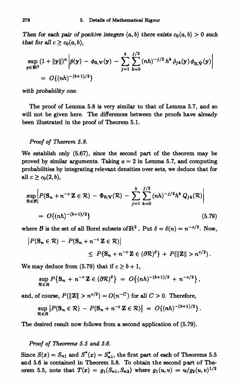
278 5. Details of Mathematical Rigour
Then for each pair of positive integers (a, b) there exists Co(a, b) > 0 such
that for all c � Co(a, b) , II j/2
yS:�2 (1 + l /yl / )a Ip(y) - 4>o.v (Y) - � E (nh)-j/2 hk Pjk (Y) 4>o.v(Y) I = O{(nh)-(b+l)/2}
with probability one.
The proof of Lemma 5.8 is very similar to that of Lemma 5.7, and so will not be given here. The differences between the proofs have already been illustrated in the proof of Theorem 5.1 .
Proof of Theorem 5.B.
We establish only (5.67) , since the second part of the theorem may be proved by similar arguments. Taking a = 2 in Lemma 5.7, and computing probabilities by integrating relevant densities over sets, we deduce that for all c � Co(2, b) ,
b j/2 sup IP(Sn + n-C Z E 'R) - �o.v('R.) - L: L: (nh)-j/2hk Qjk ('R) I �E8 j=l k=O
(5.79) where B is the set of all Borel subsets ofIR? Put fJ = fJ(n) = n-c/2 • Now,
I P(Sn E 'R.) - P(Sn + n-e Z E 'R.) I
� P{Sn + n-e Z E (81�l} + P(\ IZ I I > ne/2) . We may deduce from (5.79) that if c � b + 1 ,
sup p{Sn + n-e Z E (8'Rl} = O{ (nh)-(b+l)/2 + n-e/2 } , �ER
and, of course, P(IIZ II > ne/2) = O(n-C) for all C > O. Therefore,
sup Ip(Sn E 'R.) - P(Sn + n-e Z E 'R) / = O{(nh)-(b+1)/2 } . �ER
The desired result now follows from a second application of (5.79) .
Proof of Theore1Tl8 5.5 and 5.6.
Since S(x) = Snl and S· (x) = S�l ' the first part of each of Theorems 5.5 and 5.6 is contained in Theorem 5.8. To obtain the second part of Theorem 5.5, note that T(x) = 91 (Snl , Sn2) where 91 (U, V) = U/92 (U, v) 1/2

Nonparametric Density Estimation 279
and
Hence, with
'R(y) = { (U, V) : g2 (U, V) > 0 , g1 (U, V) � Y} ,
we have P{T(x) � y} = P{Sn E 'R(y)}. The second part of Theorem 5.5 may now be proved from the first part of Theorem 5.8, by using the argument following (5.29) in the first part of Theorem 5.1 . Likewise, the second part of Theorem 5.6 follows from the second part of Theorem 5.8. Since the Edgeworth expansions are nonstandard, we conclude with a brief account of how terms in the second expansion in Theorem 5.5 may be identified.
Define s = (nh) 1/2 , n
(nh)-l E KT { (x - Xj)/h} , j=l
0'2 (x) J1.2 (X) - hJ1.Hx) = J1.20 , p(x) = J1.l (X)/O'(x) , u2 (x) i2 (X) - hlt(x) , il; (x) = s{ij (x) - J1.j (x) }jO'(x)j .
Dropping the argument x, we have
whence
Therefore,
T ill 0'0--1
ild1 - !s-l� + i s-2� + hs-l pill } + 01' (s-3 + n-l ) .
Raising T to a power, taking expectations, and ignoring terms of order s-3 + n-1 or smaller, we deduce that
Now,
E(T) = _!S-1 E(illil2) + hS-lpE(il�) , E(T2) = E(il�) - S-l E(il��) + S-2 E(!)'� �) , E(r) = E(il:) - �S-l E(il: �) + 3hs-l pE(!)':) , E(r) E(!).t) - 2s-l E(!).t �) + 3s-2 E(!).: �) .

280
E(�:) =
E(�:) =
E(��)
E(�:�)
E(�;�)
E(���)
E(A��)
5 . Detaila of Mathematical Rigour
1 , E(�I �) = -3 (1' 1-'11 ,
-1 -3 8 (1' 1-'30 , E(A:�) = -1 -4 8 (1' 1-'21 ,
=
=
(1'-4(31-'�0 + 8-21-'40) + O(n-l ) ,
(1'-531-'201-'1 1 + 0(8-2) ,
(1'-6 {21-'�1 + 1-'201-'02) + 0(8-2) ,
8-1(1'-6(41-'1 11-'30 + 6J.t201-'21 ) + 0(8-3) ,
(1'-8 (3J.t�0J.t02 + 12J.t�1J.t20) + 0(8-2) .
Using these formulae, noting that (1'2 = 1-'20, ignoring terms of order
8-3 + n-1 or smaller, and employing identities expressing cumulants in terms of moments {see (2.6», we see that the first four cumulants of T are
1 -1 -3/2 h -1 - 2"8 J.t20 J.tll + 8 p ,
(T) -2 ( -2 6 -3 6 -2 1t4 = 8 1-'20 J.t40 - 1-'20 I-'nJ.t30 - J.t20 1-'21
+ 18J.t�03 J.t�l + 3J.t20
2 J.t02) .
(5.80)
(5.81)
All higher-order cumulaots are of order 8-3 or smaller, by an analogue of Theorem 2 .1 .
If the nonnegative integers i, j, k, l satisfy i + 2j = k + 2l, then
J.tii - J.tlcl = O(h) .
Therefore, ignoring terms of order 8-3 + n-1 or smaller,
"'2 {T) = 1 + -2 7 -3 2 '" 8 '4 1-'20 J.t3Q , (5.82)
(5.83)
Combining (5.80)-{5.83) we see that the characteristic function of T satisfies

Nonparametric Density Estimation
= e-t2/2 exp [S-1 { - � 1'203/2 J.Lllit + hpit
+ i 1'-;'03/2 (1'30 - 3J.Ll l ) (it)3 + hp(it)3} + S-2{ IJ.L203 J.L�0 (it)2
+ G 1'203 J.L�o - l2J.L202 J.L40) (it)4}] + 0(n-1 )
= e-t2/2 [1 + s-l { - ! �3/2 I'l l it + i J.L"i.i/2{J.L30 - 3J.Lll ) {it)3} + hs-l p{ it + {it)3}
+ S-2 { , ,-3 ,.2 (ot)2 + ( 2 ,,-3 ,,2 1 "-2 ,, ) (ot)4 .-20 .-30 • 3,...20 ,..30 - 12 .-20 .-40 •
+ fs J.L203 J.L�0 (it)6}] + 0(S-3 + n-l) .
281
The desired Edgeworth expansion for P{T(z) � y} follows, in a formal sense, on inverting this characteristic function.
5.5.4 Proof of Theorem 5. 7
The argument needed to prove Theorem 5.7 closely parallels that used to establish Theorem 5.3 in Section 5.3, and so will not be given in detaiL However, to indicate why the terms in the expansions have the form claimed for them we shall outline the derivation of the second part of Theorem 5.7. Put s = (nh) 1/2 ,
�j (z) = s{ij (z) - J.Lj (z) }/!T(z)j ,
� �3(X) - � J.L3(Z)!T(x)-3�2(X) .
Routine Taylor expansion gives
Hence,
• -3/2 • -3/2 8-1 A + 0 .. (8-2 + hs-1 ) , 1'20 I'll - 1'20 I'l l = L.1 .. • -3/2 • -3/2 s-1 A + 0 .. (8-2 + hs-1) . 1'20 1'30 - 1'20 1'30 L.1 ..

282 5. Details of Mathematical Rigour
Therefore, writing Va for the solution of peT $ va) = a , we have
Va - Va = -8-1 {Ql (Za ) - Ql (Za ) } + Op(8-3 + n- 1 )
_8-2 i (2y2 + 1 ) � + Op(8-3 + n-1 ) , whence
peT $ va ) = p{ T + 8-2 i (2z! + 1)� $ Va + Op(8-3 + n- 1 )} = peT' $ VI» + 0(8-3 + n-1 ) , (5.84)
where T' = T + 8-2 i (2z! + 1)�. Here we have used the delta method. All but the second of the first four cumulants of T and T' are identical up to (but not including) terms of order 8-3 + n-l ; and
var(T') = var(T) + s-2 � (2z! + 1h '2 (x) + 0(s-4 + n-1 ) .
Therefore, comparing Edgeworth expansions for T and T', peT' $ t) = peT � t) - 8-2 i (2z! + 1h '2 (x) t q,(t) + 0(s-3 + n - 1 ) .
Taking t = Va = Za + O(S-I ) and using (5.84) , we deduce that
peT $ va) = a - 8-2 i za (2z! + 1h '2 (x) q,(Za ) + 0(s-3 + n-1 ) .
Hence, changing a to 1 - CI! and noting that Zl -a = -Z"" we obtain
P{Ej(x) E -h} = peT > VI -a)
= a - 8-2 � Za (2z! + 1h '2 (x) q,(Za) + 0(s-3 + n-l ) ,
88 required.
5.6 Bibliographical Notes
Rigorous theory for bootstrap Edgeworth expansions dates from work of Singh (1981) , Bickel and Freedman (1980) , Beran ( 1982) , Babu and Singh ( 1 983, 1984, 1985) , and Hall (1986a, 1988a) . Development of expansions of coverage probability started with Hall ( 1 986a), and our work in Sections 5.2 and 5.3 is based on that contribution. The case of simple linear regression, discussed briefly in Section 5.4, is treated in greater detail by Hall (1988d). The theory for nonparametric density estimation in Section 5.5 is taken from Hall ( 1991b) .

Appendix I
Number and Sizes of Atoms of
N onparametric Bootstrap
Distribution
Let X· denote a same-size resample drawn, with replacement, from a given sample X, and let O· be the value of a statistic computed from X· . In most cases of practical interest, each distinct X· (without regard for order) gives rise to a distinct {r . For example, if {t is a mean or a variance, and if X is drawn at random from a continuous distribution, then the statement made in the previous sentence is true for almost all samples X, Le. , with probability one. In this circumstance the number of different possible values of {t equals (with probability one) the number of different possible resamples X .. .
If the sample X is of size n, and i f all elements of X are distinct, then the number of different possible resamples X· equals the number, N(n), of distinct ways of placing n indistinguishable objects into n numbered boxes, the boxes being allowed to contain any number of objects. To appreciate why, write X = {X b . . . , Xn} and let mi denote the number of times Xi is repeated in X·. The number of different possible resamples equals the number of different ways of choosing the ordered n-vector (m l , ' " , m,, ) such that each mi � 0 and mi + . . . + mn = n. Think of mi as the number of objects in box i.
Calculation of N(n) is an old but elementary combinatorial problem. In fact , N(n) = e",,-I) . One proof of this formula runs as follows. Place 2n - 1 dots in a line. Mark a cross on exactly n - 1 of the dots, and put into box i a number of objects equal to the number of dots remaining between the (i - 1)th and ith crosses, 1 5 i 5 n. (Cross 0 represents the far left of the arrangement, and cross n denotes the far right.) Each arrangement of n indistinguishable objects into n numbered boxes may be represented uniquely in this manner. Therefore, the total number N(n) of arrangements equals the number of ways of placing the n - 1 crosses among the 2n - 1 dots; this is (�:ll) , or equivalently, en;l) . See Roberts (1984, p. 42) for a similar treatment of a more general problem.
For an alternative proof, note that the number N(n) of ordered Be-
283

284 Appendix I. No. and Sizes of Atoms of Nonparam. Bootstrap Distribution
quences (mi , . . . , mn) with each mi � 0 and m1 + . . . + mn = n, equals
the coefficient of xn in (1 + x + x2 + . . . )n = ( 1 - xl-no That coefficient is
(_l)n c�n) , which is identical to en;1) .
Not all of the en; 1) atoDlB of the bootstrap distribution of 8" have equal
m8.BB. To compute probabilities, let X"(m! . . . . , mn) denote the resample
drawn from X = {Xi , . . . , Xn} in which Xi is repeated precisely mi times,
for 1 :5 i :5 n. The chance of drawing Xi out of X on a.p.y given draw equals n-i . Therefore, the chance that n draws (with replacement after
each draw) result in X* (ml ' . . . , mn) equals the multinomial probability
n! nnm1 ! . . . mn! .
IT 8* (ml " ' . , mn) denotes the value of the statistic (J* when the resa.mple
is X* (ml ' . . . , mn) , then in the circumstances discU8Sed in the first para
graph of this appendix,
(A.1) all mi � 0 with m1 + . . . + mn = n ,
for almost all samples X. These probabilities represent the atoms of the
bootstrap distribution of 8* . The right-hand side of formula (A.1) is at its largest when each rrI.i = 1,
in which case X· is identical to X. Hence, the most likely resample to
be drawn is the original sample, this event occurring with probability
Pn = n!/nn. The modal atom of the bootstrap distribution of 8· is there
fore 8, the original statistic computed from X. While X is more likely to
arise than any other resa.mple, its probability is very small for even small n, being only 3.6 x 10⁻⁴ when n = 10. The probability decreases expcr
nentially quickly with increasing n. That property reflects two features
of the bootstrap distribution of 8": the total number of atoDlB increases
rapidly with increasing sample size, and the bootstrap distribution of 8· is "smudged" very widely over these different atoDlB.
Table A.1 lists values of N(n) and Pn for different values of n. As n increases, N(n) '" (mr)-1/2 22n-1 and Pn '" (2mr) 1/2 e-n, demonstrating
that N(n) increases exponentially quickly while Pn decreases exponentially
quickly.
IT B bootstrap simulations are conducted then the chance that no re
samples are repeated is not less than
(1 - Pn) (l - 2p,,) . . . {l - (B - l) Pn} � 1 - i B(B - l ) Pn ' (A.2)

Appendix I. No. and Sizes of AtoIllll of Nonparam. Bootstrap Distribution 285
TABLE A.1 . Number of atoms, C''':I) , of bootstrap distribution, together with probability, n!/nn, of most likely or modal atom. In each case the modal value is 6, the original statistic computed from the sample.
number probability of n of atoms most likely atom
2 3 0.5 3 10 0.2222 4 35 0.0940 5 126 0.0384 6 462 1 .5 x 10-2 7 1 ,716 6.1 x 10⁻³ 8 6,435 2.4 x 10⁻³
9 24,310 9.4 x 10⁻⁴ 10 · 92,378 3.6 x 10⁻⁴
12 1,352,078 5.4 x 10⁻⁵
15 7.8 x 10⁷ 3.0 X 10⁻⁶ 20 6.9 X 10¹⁰ 2.3 X 10⁻⁸
provided (B - 1) Pn < 1 . As n and B increase,
Therefore, if B increases with n more slowly than n-1/4 en/2 - in particular, if B = O(nC) for any fixed c > 0 - then the probability that one or more repeats occur in the B values of it, converges to zero as n --+ 00 . The number of resampling operations has to increase with sample size at an exponentially fast rate before repetitions become a problem.
To be more specific, if n = 20 and B = 2, 000 then the chance of no repetitions is not less than
1 - � B(B - l) Pn = 0.954 .
This is a convenient case to remember: with a sample size of 20, and with as many as 2,000 resampling operations, the chance of repeating the same resample is less than 1 in 20. Therefore, for many practical purposes the bootstrap distribution of a. statistic 8· may be regarded 88 continuous.

286 Appendix 1. No. and Sizes of Atoms of Nonparam. Bootstrap Distribution
For sma.1l values of n , say n � 8, it is often feasible to calculate a bootstrap estimate exactly, by computing all the atoms of the bootstrap algorithm. Fisher and Hall ( 1991) discuss algorithms for exact bootstrap calculations. However, for larger samples, say n ;;:: 10, Monte Carlo simulation is usually the only practical method.
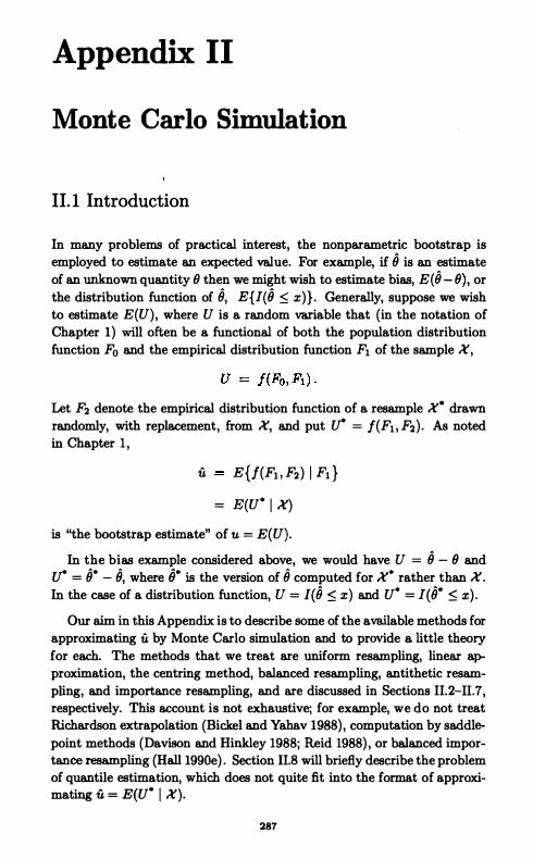
Appendix II
Monte Carlo Simulation
11. 1 Introduction
In many problems of practical interest, the nonparametric bootstrap is employed to estimate an expected value. For example, if 8 is an estimate of an unknown quantity () then we might wish to estimate bias, E(O - () , or
the distribution function of 0, E{I(8 :$ x)} . Generally, suppose we wish to estimate E(U), where U is a random variable that (in the notation of Chapter 1) will often be a functional of both the population distribution function Fo and the empirical distribution function FI of the sample X,
Let F2 denote the empirical distribution function of a resample X· drawn randomly, with replacement, from X, and put U· = f(FI , F2) . As noted in Chapter 1 ,
U E{J(Fl t F2) I FI }
= E(U· I X)
is ''the bootstrap estimate" of u = E(U).
In the bias example considered above, we would have U = 8 - () and U· = 0* - 0, where it is the version of () computed for X· rather than X. In the case of a distribution function, U = l(iJ :$ x) and U· = 1(0* :$ x) .
Our aim in this Appendix is to describe some of the available methods for approximating u by Monte Carlo simulation and to provide a. little theory for each. The methods that we treat are uniform resampling, linear approximation, the centring method, balanced resampling, antithetic resampiing, and importance resampling, and are discussed in Sections 11.2-11.7, respectively. This account is not exhaustive; for example, we do not treat Richardson extrapolation (Bickel and Yahav 1988) , computation by saddle
point methods (Davison and Hinkley 1988; Reid 1988) , or balanced importance resa.mpling (Hall 1990e) . Section 11.8 will briefly describe the problem of quantile estimation, which does not quite fit into the format of approximating u = E(U· I X).
287

288 Appendix II. Monte Carlo Simulation
11.2 Uniform Resampling
Since u is defined in terms of uniform resampling - that is, random resampling with replacement, in which each sample value is drawn with the same probability n-1 - then uniform resampling is the most obvious approach to simulation. Conditional on X, draw B independent resamples X; , . . . , xi by resampling uniformly, and let 0; denote the version of {) computed for X; rather than X. Then
B . • - B-1 ,", u· uB - � b
b=l
is a Monte Carlo approximation to U. With probability one, conditional on X, ui converges to u:.. = u as B -+ 00 .
We refer to ui as an approximation rather than an estimate. The bootstrap estimate u is based on B = 00, and only its approximate form is concerned with finite B's. Thus, we draw a distinction between the statistical problem of estimating u and the numerical problem of approximating U. While this view might seem semantic, it does help to distinguish between different approaches to inference. For example, the bootstrap approach to hypothesis testing described in Section 4.6 is concerned only with the case B = 00, since it uses the ''full'' (Le., B = 00) bootstrap estimates of quantiles and critical points. Employing a finite value of B would produce an approximation to bootstrap hypothesis testing. On the other hand, the method of Monte Carlo hypothesis testing (Barnard 1963; Hope 1968; and Marriott 1979) is concerned intrinsically with the case of finite B. For example, it is common for B = 99 to be recommended for testing at the 5% level. Thus, a Monte Carlo hypothesis test is an approximate bootstrap hypothesis test, but a bootstrap test is not a Monte Carlo test. See also Hall and Titterington (1989) .
The expected value of ui, conditional on X, equals u:
B B E(ui I X) = B-1 L E(U; I X) = B-1 L u U .
b=l b=l
Therefore, ui is an unbiased approximation to u, and the performance of u; may be reasonably described in terms of conditional variance,
In many problems of practical importance, var(U· I X) is asymptotic to either a constant or a constant multiple of n- 1 , as n -+ 00. For example, if

Uniform Resampling 289
we are estimating a distribution function then U· is an indicator function, and so U·2 = U· , whence
var(U· I X) = 11(1 - 11) -+ Uo(l - Uo) , where Uo (typically a value of a Nonnal distribution function) equals the limit as n --+ 00 of 11. IT we are estimating bias and fJ = g(X) is a smooth function of a d-variate sample mean, then U· = o· - fJ = g(X·) - g(X) , where X· is the resample mean. By Taylor expansion,
d U· = g(X· ) - g(X) � E (X· - X)(j) g; (X) , (A.3)
;=1 where x(j) = (x)U) denotes the jth element of a d-vector x and
gj (x) = (8/8xU» ) g(x) .
Thus,
where
d var(U· I X) = var{ E (X· - X) (j) gj (X) I X} + O(n-2)
j=1
d 2 E { E (X - JI.) (j) gj (JI.) } ;=1
(as n --+ 00) and JI. = E(X) is the population mean.
These two examples describe situations that are typical of a great many that arise in statistical problems. When the target 11 is a distribution function or a quantile, the conditional variance of the uniform bootstrap approximant is roughly equal to CB-l for large n and large B; and when the target is the expected value of a smooth function of a mean, the variance is approximately C B-1 n -1 . In both cases, C is a constant not depending on B or n. Efficient approaches to Monte Carlo approximation can reduce the value of C in the case of estimating a distribution function, or increase the power of n-l (say, from n-l to n-2) in the case of estimating the expected value of a smooth function of a mean. Most importantly, they usually do not increase the power of B-1 • Therefore, generally speaking, even the more efficient of Monte Carlo methods have mean squared error that decreases like B-1 as B increases, for a given sample.

290 Appendix II. Monte Carlo Simulation
11.3 Linear Approximation
We motivate linear approximation by considering the bias estimation example of the previous section. Suppose our aim is to approximate
u = E(U* ' X) , where
u· = O· - 0 = g(X·) - g(X) and 9 is a smooth function of d variables. Let us extend the Taylor expansion (A.3) to another term,
d U· = E (X· - X)(j) gj (X) j=1
d d + � E L (X· - X)(j) (X· - X) (1c) gj1c (X) + . . . , (A.4)
j=1 1c=1 where gj, ... jr (x) = (8'" 18x(j, ) . . . 8x(Jr » g(x) . As we noted in Section 11.2, the conditional variance of U· is determined asymptotically by the variance of the first term on the right-hand side of (A.4) , which is the linear component in the Taylor expansion. Now, our aim is to approximate E(U* I X) , and the linear component does not contribute anything to that expectation:
d E {� CX· - X) (j) gj (X) I X}
d = E E{ (X· - X) (j) I X} gj (X) = O . (A.5)
j=1
Therefore, it makes sense to remove the linear component; that is, base the uniform resampling approximation on
d V· = U· - E (X· - X) (j) gj (X) ,
j=1 instead of on U· . Conditional on X, draw B independent resamples X; , . . . , X; by resampling uniformly (exactly as in Section 11.2) and put
d V; = U; - E CX; - X)(j) gj (X)
j=1 d
g(X;) - g(X) - 2: (X; - X)(j) gj (X) , j=1

Linear Approximation 291
1 � b � B, where X; denotes the mean of the resample X; . Define
B • • - B- 1 '" v· vB - L..J b ·
b=1
Then v; is the linear approximation method approximation of u. With probability one, conditional on X, v; -+ ii. 88 B -+ 00.
In view of (A.5) , E(V* I X) = E(U· I X) = ii., and so v; is an unbiased approximant of ii.. The conditional variance of v; is dominated by that of the first remaining term in the Taylor expansion, just 88 in the case of ii.;,
var( v; I X) = B-1 var(V· I X) ,
and
var(v· 1 X)
with probability one as n -+ 00, where1
d d d d
(A.6)
tJ � L L L L Bj, kt (X) Bhk2 (X) fTith fTktk2 , (A.7) it=1 kt =1 h=1 k2=1
n fT;k
= n-1 L (Xi - X)(j) (Xi - X)(k) . (A.8)
i=1 Therefore, the order of magnitude of the variance has been reduced from B-1 n-1 (in the case of ii.;) to B- 1 n-2 (in the case of v;). The numerical value of the reduction, for a given problem and sample, will depend on values of the first and second derivatives of B, as well as on the higherorder terms that our asymptotic argument has ignored.
More generally, we may approximate U· by an arbitrary number of terms in the Taylor expansion (A.4) , and thereby compute a general "polynomial approximation" to u. For example, if m � 1 is an integer then we may define
l In Hall (1989a) , the factor 1 was inadvertently omitted from the right-hand side of (A.7) .

292 Appendix II. Monte Carlo Simulation
(a generalization of V;) ,
and B
B-1 L W; + w . • * wB
1>=1 Then wi is an unbiased approximation of u. Of course, the approximation is only practicable if we can compute w, which is a linear form in the first m central sample moments, with coefficients equal to the derivatives of g. In the special case m = 1, wi reduces to our linear approximation vi, and there til = O. The conditional variance of wi is of order B-1 n-(m+l) as n -+ 00. Of course, w; -+ U as B -+ 00, for fixed X. If the function 9 is analytic then for fixed X and B, w; -+ u as m -+ 00. Each of these limits is attained with probability one, conditional on X.
Monte Carlo methods based on functional approximation have been discussed by Oldford (1985) and Davison, Hinkley, and Schechtman (1986) .
11.4 Centring Method
To motivate the centring method approximation, recall that the linear approximation method produces the approximant
B vi = B-1 L V;
&=1 B d
B-1 L {g(X;) - g(X) - L (X; - X) (j) g; (X) } &=1 ;=1
d * ""'
- . - (j) -UB - L (X. - X) g; (X) , ;=1
where u; is the uniform resampling approximation of u and
B X: = B-1 L X;
&=1 is the grand mean of all the resamples. Now,
d E (X.* - X)(j) g; (X) � g(X.* ) - g(X) , ;=1

Balanced R.esampling 293
by Taylor expansion, and so
. -:CB ' where B
B-1 E g(X;) - g(x.: ) . h=1
We call xi the centring method approximation to U. It differs from ui in that the mean of the g(X;)'s is now centred at g(X:) rather than g(X) ; reca.ll that
B ui = B-1 L g(X;) - g(X) .
b=1 The centring method approximation was suggested by Efron (1988) .
As expected, xi -+ u as B -+ 00, conditional on X. The approximant xi is not unbiased for u, although the bias is generally very low, of smaller order than the error about the mean. Indeed, it may be proved that
E(xi I X) - u = -(Bn)-l & + O{(Bn)-2} ,
var(xi I X) = (Bn2)- 1 /3 + O{(Bn)-2 + (Bn3)-1 } , with probability one as n -+ 00 , where
d d • 1 '" '" - . 'Ie a = 2" � � gjle (X) fT3 ,
j=1 1e=1
(A.9)
(A. 10)
(A.ll)
and /3, ilile are given by (A.7) and (A.8) , respectively. See Hall (198980) . Note particularly that by A.6) and (A. I0) , the conditional asymptotic variances of vi and xi are identical. Since vi is an unbiased approximant and the bias of xi is negligible relative to the error about the mean (order B-1 n- l relative to B-l/2 n- l ) , then the approximations vi and xi have asymptotically equivalent mean squared error.
11.5 Balanced Resampling
H we could ensure that the grand mean of the bootstrap resamples was identical to the sample mean, Le.,
X· = X . , (A. 12)
then the uniform approximation ui, the linear approximation vi and the centring approximation xi would all be identical. The only practical way of guaranteeing (A.12) is to resample in such a way that each data point Xi occurs the same number of times in the union of the resamples X; .

294 Appendix II. Monte Carlo Simulation
To achieve this end, write down each of the sample values Xl , . . . , X.. B times, in a string of length Bn; then randomly permute the elements of this string; and finally, divide the permuted string into B chunks of length n, putting all the sample values lying between positions (b - l)n + 1 and bn of the permuted string into the bth resample xt, for 1 � b � B. This is balanced resampling, and amounts to random resampling subject to the constraint that Xi appears just B times in U" xl. Balanced resampling was introduced by Davison, Hinkley, and Schechtman (1986) , and high-order balance has been discussed by Graham, Hinkley, John, and Shi (1990) . See also Ogbonmwan and Wynn (1986, 1988) . An algorithm for performing balanced resampling has been described by Gleason (1988) . The method of Latin hypercube sampling (McKa.y, Beckman, and Conover 1979; Stein 1987) , used for Monte Carlo simulation in a nonbootstrap setting, is closely related to balanced resampling.
The balanced resampling approxima.tion of u = E{g(X*) I X} is
B u� ;: B-1 �-g (xt) .
b=1
where xt denotes the mean of xt . Once again, u� -. u as B -> 00, with probability one conditional on X. The balanced resampling approximation shares the asymptotic bias and variance formulae of the centring approximation xi, introduced in Section II.4,
(A. 13)
(A.14)
with probability one as n -. 00, where a, /3 are given by (A. 11 ) and (A.7) , respectively; compare (A.9) a.nd (A. 10) . In particular, in the context of bias estimation for a smooth function of a mean, balanced resampling reduces the orders of magnitude of variance and mean squared error by a factor of n-1 • Formulae (A.13) and (A. 14) are not entirely trivial to prove, and the asymptotic equivalence of bias and variance formulae for the centring method a.nd balanced resampling is not quite obvious; see Hall (1989a) .
In Sections 1I.3 and II.4, and so far in the present section, we have treated only the case of approximating a smooth function of a mean. The methods of linear approximation and centring do not admit a wide range of other applications. For example, linear approximation relies on Taylor expansion, and that demands a certain level of smoothness of the statistic U. However, balanced resampling is not constrained in this way, and in principle applies to a much wider range of problems, including distribution

Balanced Resampling
function and quantile estimation. In those cases the extent of improvement of variance and mean squared error is generally by a constant factor, not by a factor n-I •
Suppose that U is an indicator function of the form U = I(S :5 x) or U = I(T :5 x) , where S = nl/2 (9 - (J)/u and T = n1/2 (9 - (J)/fF are
statistics that are asymptotically Normal N(O, 1 ) . The bootstrap versions are
U· = I(S· :5 x) and u· = I(T· :5 x) ,
respectively, where
and
(The pros and cons of pivoting are not relevant to the present discussion.) To construct a balanced resampling approximation to u = E(U· I X), first
draw B balanced resamples xt, 1 :5 b :5 B, as described two paragraphs
earlier. Let 9t, fFt denote the versions of 9, fF respectively computed from
xt instead of X, and put
and
ut = I (St :5 x) or I(Tt :5 x) , depending on whether U = I(S :5 x) or I(T :5 x) . (We
define Tt = c, for an arbitrary but fixed constant c, if ut = 0.) The balanced resampling approximation to u is
B · t _ B-I ""' Ut uB - L..J & .
&=1
Recall from Section 11.2 that the uniform resampling approximation u� is unbiased for u, in the sense that E(u� I X) = u, and has variance
var(u� I X) = B-I u(l - u) '" B-1 �(x) {l - �(x)}
as n -+ 00. The balanced resampling approximant is slightly biased, although the bias is low relative to the error about the mean,
E(u1 1 X) - u = D(B-I )
with probability one. The asymptotic variance of u1 is less than that of u� by a constant factor p(X)-l < 1, since

296 Appendix II. Monte Carlo Simulation
see Hall (1990a) . Thus, the asymptotic efficiency of balanced resampling relative to uniform resampling, in this context, is '
which reaches a maximum at x = 0 and decreases to 1 as Ix l 1 00. See Hall ( 1990a) .
The same asymptotic efficiencies apply to the case of quantile estimation, which we discuss in more detail in Section 11.8. Figure A. l graphs the efficiencies.
II.6 Antithetic Resampling
The method of antithetic resampling dates back at least to Hammersley and Morton (1956) and Hammersley and Mauldon (1956) . See Snijders (1984) for a recent account in connection with Monte Carlo estimation of probabilities. Antithetic resampling may be described as follows. Suppose we have two estimates {h and O2 of the same parameter fJ, with identical means and variances but negative covariance. Assume that the costs of computing 01 and O2 are identical. Define 03 = � (01 + O2 ) , Then 03 has the same mean as either 81 or O2 , but less than half the variance, since
1 • • • •
= :d var 01 + var O2 + 2COV(01 , (2) } = Hvar(8d + cov(81 , 82 ) } < �var(8d .
Since the cost of computing 83 is scarcely more than twice the cost of computing either {h or 82 , but the variance is more than halved, there is an advantage from the viewpoint of cost-effectiveness in using 83 , rather than either 81 or 82 , to estimate O. Obviously, the advantage increases with increasing negativity of the covariance, all other things being equal.
To appreciate how this idea may be applied to the case of resampling, let U· denote the version of a statistic U computed from a (uniform) resample X· = {X; , . . . , X�} rather than the original sample X = {Xl , . . . , Xn} . Let 7r be an arbitrary but fixed permutation of the integers 1 , . . . , n, and let il , . . . , in be the random integers such that X: = Xi, for 1 � i � n.
Define X:* = X7r(j,) , 1 � i � n, and put X .... = {X;· , . . . , X=* } . That is, X·· is the (uniform) resample obtained by replacing each appearance of Xk in X· by X,..(k) . If U" denotes the version of U computed from X·" instead of X, then U" and U·· have the same distributions, conditional on X. In particular, they have the same conditional mean and variance. If we choose the permutation 7r in such a way that the conditional covariance

Antithetic Resampling 297
of U· and U·· is negative, we may apply the antithetic argument to the pair (U· , U·· ) . That is, the approximant
UC = � (U. + UU) will have the same conditional mean as U· but less than half the conditional variance of U· .
If the Xi 'S are scalars then in many cases of practical interest, the "asymptotically optimal" permutation 11" (which asymptotically minimizes the covariance of U· and UU) , is that which takes the largest Xi into the smallest Xi , the second largest Xi into the second smallest Xi , and so on. That is, if we index the X/s such that Xl $ . . . $ Xn, then 1I"(i) = n - i + l for 1 $ i $ n. For example, this is true when U = g(X) - g(p,) , where 9 is a smooth function, and also when
(A.15)
The asymptotically optimal permutation 11" in the case of a d-dimensional sample, where U = g(X) - g(p.) or
U = I [ nl/2 {g(X) - g(p)} $ x ] , is that one that reverses the order of the quantities
d Yi = L (Xi - X)(j) g(j) (X) , 1 $ i $ n .
j=l
(A.16)
That is, if we index the Xi 's such that Yl $ . . . $ Yn, then 11" ( i) = n - i + 1. We shall call 11" the antithetic permutation. These results remain true if we Studentize the arguments of the indicator functions at (A.15) and (A. 16) ; the pros and cons of pivoting do not have a role to play here. The reader is referred to Hall (1989b) for details.
The method of antithetic resampling may be used in the following way to approximate the bootstrap estimate u = E(U· I X) . Draw B independent, uniform resamples X; , 1 $ b $ B; by applying the antithetic permutation, convert X; into the corresponding antithetic resample X;· ; compute the versions of U; and U;· for X; and X;" , respectively; and define
B u: = � B-l L (U; + U; .. ) .
b=l
Note that u: is an unbiased approximant of u, in the sense that
E(u: I X) = u . The conditional variance of u: is given by
var(u! I X) = (2B)-1 {var(U" I X) + cov(U" , U·" I X)} ,

298 Appendix II. Monte Carlo Simulation
where (U* , U**) denotes a generic pair (U; , U;") . In general, as n --+ 00,
var(u: I X) = q var(ui I X) + o{var(ui I X) } ,
where 0 � q < 1 .
The exact value of q depends on the situation, i t being greater for less
symmetric distributions. For example, in the case of distribution function
estimation where u = P(S" � x I X) or peT"' � x I X) , the value of
q = q(x) = lim lim {var(u: I X)/var(ui I X) } n--+(Xl B-+oo
is an increasing function of both Ixl and the skewness of the sampling
distribution. The minimum value q = 0 can only arise in this context when
both x = 0 and the sampling distribution has zero skewness.
Thus, generally speaking, antithetic resampling reduces variance by a
constant factor. In this respect, balanced resampling is superior in the
case of approximating the conditional mean of a smooth function, since it
reduces variance by a factor that converges to zero as sample size increases.
Again, the reader is referred to Hall (1989b) for details.
II.7 Importance Resampling
II. 7. 1 Introduction
The method of importance resampling is a standard technique for improv
ing the efficiency of Monte Carlo approximations. See Hammersley and
Handscomb (1964, p. 60ff) . It was first suggested in the context of boot
strap resampling by Johns (1988) and Davison (1988) . The account in this
section differs from Johns' and Davison's.
We show that the improvements offered by importance resampling are
asymptotically negligible in the contexts of bootstrap bias estimation and
variance estimation, but that they can be substantial when distribution
functions or quantiles are the subject of interest. Hinkley and Shi (1989) ,
Hall (1991a) , and Do and Hall (1991) have also discussed importance re
sampling.
Our aim in this section is to give a general account of importance
resampling, so that its application to a wide variety of problems such as
bias estimation, variance estimation, and quantile estimation may be con
sidered. On grounds of efficiency relative to uniform resampling, there is little reason to consider importance resampling in the cases of bias and
variance estimation, but that negative result is not clear without a rea-

Importance Resampling 299
sonably general analysis of the method. Subsection 11.7.2 will introduce
and develop the principle of importance resampling, and subsections II. 7.3 and I1.7.4 will apply the principle to bias estimation, variance estimation,
and distribution function estimation. The empirical approach to impor
tance resampling described in subsection I1.7.4 below is drawn from Do
and Hall ( 1991 ) .
II. 7. 2 Concept of Importance Resampling
Let X = {XI , ' " , Xn} denote the sample from which a resample will be
drawn. (This notation is only for the sake of convenience, and in no way precludes a multivariate sample. ) Under importance resampling, each Xi is assigned a probability Pi of being selected on any given draw, where
�Pi = 1 . Sampling is conducted with replacement, so that the chance of
drawing a resample of size n in which Xi appears just mi times (1 :::; i :::; n) is given by a multinomial formula,
n! n --;------:c II p'!'i . md . . . mn ! i=1
Of course, � mi = n. Taking Pi = n - 1 for each i , we obtain the uniform
resampling method of Section 11.2.
The name ''importance'' derives from the fact that resampling is de
signed to take place in a manner that ascribes more importance to some
sample values than others. The aim is to select the Pi 'S so that the value assumed by a bootstrap statistic is relatively likely to be close to the quantity
whose value we wish to approximate.
There are two parts to the method of importance resampling: first,
a technique for passing from a sequence of importance resamples to an
approximation of a quantity that would normally be defined in terms of
a uniform resample; and second, a method for computing the appropriate
values of Pi for the importance resampling algorithm. One would usually
endeavour to choose the Pi 'S so as to minimize the error, or variability, of
the approximation.
We know from Appendix I that there are N = enn-1) different possible
resamples. Let these be Xl , ' " , X N , indexed in any order, and let mii denote the number of times Xi appears in Xi ' The probability of obtaining
Xi after n resampling operations, under uniform resampling or importance resampling, equals
7rj =
n! ----- n-n mid . . . mjn !

300
or
Appendix II. Monte Carlo Simulation
n! n n 11'.1 = I , II p'('i' = 1I'i II (np,)m.1' , (A. 17) mil . . . . min ' ;=1 i=l
respectively. Let U be the statistic of interest, a function of the original sample. We wish to construct a Monte Carlo approximation to the bootstrap estimate u of the mean of U, U = E(U) .
Let X· denote a resample drawn by uniform resampling, and write U· for the value of U computed for X· . Of course, X· will be one of the Xi 's. Write ui for the value of U· when X· = Xi ' In this notation,
N N n U = E(U* I X) = E Uj 1I'i = E ui 1I'j II (np,)-mj, ,
j=l j=l ,=1
the last identity following from (A. 17) .
(A.18)
Let xt denote a resample drawn by importance resampling, write Ut
for the value of U computed from Xt , and let M! he the number of times Xi appears in xt . Then by (A. 18) ,
Therefore, it is possible to approximate u by importance resampling. In
particular, if xt, 1 :::; b :::; B, denote independent resamples drawn by importance resampling, if ut equals the value of U computed for xt , and if M� denotes the number of times Xi appears in xt , then the importance resampling approximant of u is given by
B n uk = B-1 E ut II (npi)-Ml, .
b=l ;=1
This approximation is unbiased, in the sense that E(uk I X) = U. Note too that conditional on X, uk -- u with probability one as B -- 00.
If we take each Pi = n-1 then uk is just the usual uniform resampling approximant ui . We wish to choose PI , . . . , Pn to optimize the performance of uk. Since uk is unbiased, the performance of uk may be described in terms of variance,
where
var(uk l X) = B-1 var{ ut II (npi)-M�. I X} B-l (v _ u2) , (A.19)

Importance Resampling
N n = L 11".1 U� II (np,) -2mJ'
;=1 i=1 N n
= L 11"; U� II (np.)-mJ' ;=1 i=1
301
(A.20)
On the last line, Mi· denotes the number of times Xi appears in the uniform resample X· . Ideally we would like to choose Pl , . . . , Pn so as to minimize V(pl l . . . , Pn) , subject to L:Pi = 1. Subsections 11.7.3 and 11.7.4 below treat special cases of this problem.
II. 7.3 Importance Resampling for Approximating Bias,
Variance, Skewness, etc.
Let 0 denote an estimate of an unknown parameter 80 , calculated from the sample X, and write 0* for the version of 0 computed from a uniform
resample X· . Take U = (0 - 80)k and U· = (0* - O)k, where k is a positive integer. In the cases k = 1 , 2, and 3, estimation of U = Uk = E(U) is essentially equivalent to estimation of bias, variance, and skewness, respectively, of which the bootstrap estimate is U = Uk = E(U· I X) . There are some minor differences of detail; for example, 1"'J strictly equals mean squared error rather than variance, the latter being 1"'J - u't. However, the
importance resampling approximation to � - � has the same asymptotic properties as the approximation to �, and so it is appropriate to focus attention on approximating �. We shall prove that there are no asymptotic advantages in using importance resampling rather than uniform resampling to approximate Uk .
Again we assume the "smooth function model" introduced in Section 2.4.
Thus, the sample values Xi are d-variate with population mean J.' = E(X) , and 80 , 0 may be represented by 80 = g(p) , fJ = g(X) , where g is a smooth real-valued function of d variables. Define 0, = - log(npi) .
n d 2 iI2 = n-1 L { L (Xi - X)(j) 9; (X) } ,
i=1 ;=1 d
E, = n- 1/2 iI-1 L (X. - x)(j) 9j (X) . ;=1
(A.21)

302 Appendix II. Monte Carlo Simulation
Write Mi· for the number of times X. appears in X·. Then
d U· = {g(X· ) - g(X) }k � { L (X· - X)(j) gj (X) t
whence by (A.20) ,
j=1 n k ( -1/2 . '" M. .) n U L.J i f. , i=1
v = E{
U·2 � (npi ) -M: I X} { ( n ) 2k n
} {n-1/2 U)2k E t; Mi· Ei 1] (npi)-Mt I X
(n-l/2 u)2k E(V�k eV� I X) ,
where VI = L: M: Ei , V2 = L: M: 6, .
(A.22)
Conditional on X, the vector (M; , . . . , M�) has a multinomial distribution with all probabilities equal to n-1 , and so
E(M; I X) = 1 , var(M; I X) = E(M; M; I X) = 1 - n-1 •
It is now readily proved by a central limit theorem for weighted multinomials (for example, in Holst 1972) that conditional on X, (VI , V2) is asymptotically Normally distributed with mean ( 0, L: 6i) , variances ( 1 , L: 6� - n-I (L: 6i)2 ) , and covariance L: Ei /5o. Here we have used the fact that � E,; = 0 and L: E� = 1. The constraint L: Pi = 1 implies that L: 6i = � L: 61 + 0(1) and n-1 (L: 6i )2 -+ O. Therefore, defining S2 = L: 61 and p = 8-1 L: Ei 6,; , we have
v (n-I/2 U)2k E(N�k eN2 1 X) = (n- Ij2 U)2k E{ (Nl + Sp2 )2k I X} e·2 , (A.23)
where conditional on X, (NI ' N2) is bivariate Normal with means (0, l s2) , variances ( 1 , S2) , and correlation p. The right-hand side of (A.23) is minimized by taking 8 = 0, Le., 6i = 0 for each i, which is equivalent to demanding that each Pi = n - 1 .
Therefore, the minimum asymptotic variance of the importance resampiing approximant occurs when each Pi = n- 1 , and in view of (A.19) and (A.23) is given by
B-1 (v _ 112) IV B-1 (n-1/2 U)2k {E(N2k) _ (ENk)2 } ,
where N has the Standard Normal distribution.

Importance ResampJing 303
II. 7.4 Importance Resampling for a Distribution Function
In the case of estimating a distribution function there can be a significant advantage in choosing nonidentical Pi 'S, the amount of improvement depending on the argument of the distribution function. To appreciate the extent of improvement we shall consider the case of estimating the distribution function of a Studentized statistic,
assuming the smooth function model. Other cases, such as that where S = nl/2 (iJ - 80)/(1 is the subject of interest, are similar; the issue of Studentizing does not play a role here.
Use notation introduced in subsection II.7.3 above, and take
where
(We agree to define T* = c, for an arbitrary but fixed constant c, in the event that ft .. = 0.) Now, oil = P(T- $ x I X) , and for this particular x we wish to choose Pl , . . . , Pn to minimize
There are two practical solutions to this problem, one of them asymptotic and the other empirical. We first treat the asymptotic solution.
Define f,;, 6i , Mi" , Vl ' V2 , Nl , N2 , 8, and p 88 in the previous subsection, and note that T- � E M; fi . Then, by arguments similar to those in (A.22) and (A.23) ,
v '" E{ l (� Mi- fi � x) !! (npi)-M; I X} E{I(Vl � x) eV2 I X} E{ I(Nl � x) eN2 I X} C)(x - sp) e·2 •

304 Appendix II. Monte Carlo Simulation
The values of s and p that minimize �(x - sp) ea2 are (s, p) = ±(A, I) ,
where A = A(x) > 0 is chosen to minimize �(x - A) eA2 • Taking 6i = Afi + C, where C is chosen to ensure that EPi = n-1 E e-6, = 1 , we see that s -+ A and p -+ 1 .
Therefore, the minimum asymptotic variance of the importance resampIing approximant occurs when
Pi = ",n -AEj , L.Jj=l e l $ i $ n ,
where fi is given by (A.21) . This minimum variance is
since ii. -+ �(x) as n -+ 00 .
(A.24)
(A.25)
Writing v for V(p1 , . . . , Pn) , we see that the extent of improvement offered by this approach is given by
variance of ua (under uniform resampling) rex) =
variance of fL � (under importance resampling)
B-1 (fL - fL2) B-1 (V - fL2)
�(x){1 - �(x) ) A2 •
�(x - A) e - �(X)2
(To obtain the second identity, note that the conditional variance of fLa equals B-1 (u - fL2) since v = fL when each Pi = n -1 . To obtain the last asymptotic relation, use (A.25) and observe that fL-fL2 -+ �(x) { l- �(x)}.) Values of A = A(x) that maximize rex) , and of rex) for this choice of A, are given in Table A.2.
Note that r is a strictly decreasing function, with r( - 00) = 00,
reO) = 1 .7, and r(+oo) = 1 . Therefore, importance resampling can be considerably more efficacious for negative x than positive x. If we wish to approximate G(x) = P(T" $ x I X) for a value of x > 0, it is advisable to work throughout with -T* rather than T* and use importance resampling
to calculate
P(-T· $ -x I X) = 1 - G(x) .
Next we describe an empirical approach to selecting the optimal Pi'S for importance resampling. Divide the program of B simulations into two parts, involving B1 and B2 simulations respectively, where B1 + B2 = B.

Importance Resampling
TABLE A.2. Optimal values of A = A(x) and values of asymptotic efficiency r(x) for selected x (taken to be quantiles of the Standard Normal distribution) .
�(x) A(x) rex)
0.005 2.6561 69.0 0.01 2.5704 38.0 0.025 2.1787 17.6 0.05 1 .8940 10.0 0. 1 1 .5751 5.8 0.5 0.6120 1 .7 0.9 0.1 150 1 .1 0.95 0.0602 1 . 1 0.975 0.0320 1 .0 0.99 0.0139 1 .0 0.995 0.0074 1 .0
305
Conduct the first BI simulations by uniform resampling, and thereby approximate v by
B, n BII L I (T; � x) II (npi)-M;"
b=l i=l
where T; denotes the value of T* computed for the uniform resample X; , 1 � b � BI . Choose PI , . . ' , Pn to minimize VB" subject to .EPi = 1 . Conduct the remaining B2 simulations by importance resampling, using the Pi'S that minimize VB, . Approximate u = G(x) = P(T- � x I X) from the BI uniform resamples and the B2 importance resamples, obtaining GI (x) and G2 (x) where
B, UB, = BI I L I(T; � x) ,
b=l B2 n
G2 (x) = Bi l L I(T;- � x) II (npi)-M;: , b=l i=l
and T;* is the value of T computed from the bth importance resample X;* . Finally, combine these approxima.tions to obtain
O(x) = p G1(x) + (1 - {j) 02(x) ,

306 Appendix II. Monte Carlo Simula.tion
where
(3 = max [{ �n VB, (P) - 11�J{11B' + rnJn VB, (P) � 211�J -\ 0 ] .
(The latter is an estimate of var( 62 I X) / {var( 62 I X) + var( 61 I X) } . )
II.B Quantile Estimation
Here we consider the problem of estimating the ath quantile, {"" of the distribution of a random variable R such as S = n1/2 (8 - 80)/(7 or T = n1/2 (O - 80}/&. We define {'" to be the solution of the equation
P(R :5 {"') = a .
Now, the bootstrap estimate of e", is the solution �'" of
peR" :5 t", I X} = a , (A.26)
where (if R = S)
or (if R = T) .
The equation (A.26) usually cannot be solved exactly, although, as pointed out in Appendix I, the error will be an exponentially small function of n. For the sake of definiteness we shall define
t", = ii-I (a) = inf{x : H(x} � a} ,
where H(x) = P(R" :5 x I X). (A.27)
Approximation of the function ii(x} falls neatly into the format described in earlier sections, where we discussed Monte Carlo methods for approximating a conditional expectation of the form 11 = E(U· I X). Take
U" = I (R* :5 x) and apply any one of the methods of uniform resampling,
balanced resampling, antithetic resampling, or importance resampling to obtain an approximation iiB (x) to H(x) . Then, following the prescription suggested by (A.27) , define
� - 1 -{"" B = HE (a) = inf{x : Hb(x) � a} . (A.28)
For each of these methods, the asymptotic performance of t"" B as an approximation to t", may be represented in terms of the performance of HB(�"'} as an approximation to H (e", } = a, by using the method of Bahadur representation,

Quantile Estimation 307
where of course t/J is the Standard Normal density and -'a the a-Ievel Standard Normal quantile. See Hall (1990&, 1991a) . (Note from subsection II.7.4 that if a > 0.5 and we are wring importance resampling, it is efficacious to approximate instead the (1 - a)th quantile of -T* , and then
change sign.) This makes it clear that the asymptotic gain in performance obtained by
wring an efficient resampling algorithm to approximate ii-l (a) is equivalent to the asymptotic improvement when approximating ii(z) at the point z = (a' In the case of importance resampling, where optimal choice of the resampling probabilities Pi depends very much on the value of (a, one implication of this resUlt is that we may select the Pi'S as though we were approximating ii(za) (bearing in mind that (a ..... -'a as n ..... 00). Alternatively, we might construct an approximation ea of (a via a pilot program of uniform resampling, and then select the Pi 'S as though we were approximating ii{ea)'
A graph of the efficiency, relative to uniform resampling, of a distribution or quantile approximation by Monte Carlo means, is typically a bell-shaped or similar curve that asymptotes to unity in the tails. This means that the efficiency is greater towards the centre of the distribution than in the tails, where it is most often needed for constructing confidence intervals or hypothesis tests. An exception to this rUle is importance resampling, where the efficiency curve is cup-shaped, lowest at the centre of the distribution and diverging to +00 in either tail; see Figure A.l . That observation demonstrates the considerable potential of importance resampling for quantile estimation.
Formula (A.28) generally produces an approximation (a,B that is identical to one of the resampled values of R* . In the case of uniform resampling, careful choice of B can enhance the coverage accuracy of a confidence interval obtained by wring this quantile approximation. Let R;, . . . , R;' denote the B values of R* obtained by uniform resampling, and suppose we choose B and II such that
II/{B + l) = a .
In the case a = 0.95 this would involve taking B = 99, 199, . . . instead of B = 100, 200, . . . , respectively. Since the B values of R* divide the real line into B + I, not B, parts, then it makes sense to select ea,B as the 11th largest of R;, . . . , Ri.
This definition of (a,B may be justified more fully as follows. We wish to estimate (a, which has the property
peR S (<II) = a = II/{B + 1) .
If we use the approximant (a,B in place of (<II in a formula for a one-sided

308 Appendix II. Monte Carlo Simulation
1 4
1 2 antithetic
1 0
8
6
4
2
a -2 .0 -1 .5 - 1 .0 -0.5 0.0 0.5 1 .0 1 .5
FIGURE A. 1 . Asymptotic efficiencies of balanced resampling, antithetic resampling, and importance resampling for approximating the bootstrap distribution function
H(x) = P{R- :5 x I X), where R- = S- or T· . The horizontal axis represents x. The same efficiencies apply to approximation of the bootstrap quantile ta = H-l {o) , when 0 = 4)(x) . Each curve represents a plot of the function
e(x) = lim lim [var{H;(x) I X}jvar{HB(X) I X}) , fl�OO B ...... oo
where H; (x) denotes the approximation after B simulations of uni
form resampling and ii B (x) is the approximation after B simulations of balanced resampling, antithetic resampling, or importance resampIing respectively. In the case of balanced resampling, e{x) = p(x) , where the latter is defined in Section 11.5. For antithetic resampiing, e(x) = q{x)-t , where q(x) is defined in Section 11.6. (We have plotted the most favourable case for antithetic resampIing, in which the sampling distribution is symmetric.) For importance resampIing, e(x) = rex), where the latter is defined in subsection 11.7.4. The methods of balanced and importance resampling may' be combined to produce a new method that improves on both the other two; see Hall (1990e).
2.0

Quantile Eatimation 309
confidence interval of the form (8 - i, 00) , then the coverage probability of that interval will be peR $ (OI,B) rather than a. To appreciate the size of the error peR $ (OI,B) - a, define p = P(R- $ R I X). Conditional on X, let the random variable N have the binomial Bi(B, p) distribution. (We put a circumflex on p simply to indicate that p is a random variable.) Let R{l) $ �·2) $ . . . $ R{B) denote the values R;, . . . , Ri arranged in order of increasing size. Then (OI,B = R{JI) is our uniform resampling approximation to (OI ' and
P(R $ {OI,B I X) = P( at m08t ll - l out of Ti, . . . , Ts are < R I X)
= P(N $ II - 1 1 X)
= E (�) pi (l - p)B- . j=O J
Therefore,
P(R $ (OI,B) = E{P(R $ {OI,B I Xl }
= E (�) t pi(l - p)B-; dP(p $ p) . j=O J 10 (A.29)
To elucidate formula (A.29) , recall that R denotes either nl/2 (8 - Bo)/u or nl/2 (O - Bo)/fr, and that H(x) = peR· $ x I X) denotes the bootstrap distribution function of R· . If R = nl/2(0 - Bo)/fr then
pcp $ p) P{F(R) $ p} = P{R $ F-1(p)}
= P{Bo E (0 - n-1/2 li {", 00) } . That is, Pcp $ p) equals the coverage probability of a nominal Jrlevel percentile-t confidence interval for 80, and so
where An is a function of bounded variation. See subsection 3.5.4. In the case R = n1/2 (8 - Bo)/u we have

310 Appendix II. Monte Carlo Simulation
for another function An of bounded variation. Therefore, by (A.29),
peR � (o,B) = � (�) f pi (1 - p)B-i d{p + An(P)}
,=0 J
where
= v(B + 1)-1 + n-1 Pn(B, v) ,
Pn(B, v) = f K(P) dAnCP) ,
K(P) = E (�) pi(l - p)B-i .
i=O J
(A .30)
(Note that f K(P) dp = v(B+1)-1 , and that Pn(B, v) is bounded uniformly in B and v.) Formula (A.30) makes it clear that v(B + 1)-1 should reasonably be regarded 88 the nominal value of the probability peR � (o,B) , and 80 provides a theoretical underpinning for the definition of (o,B given two paragraphs earlier.
We claim that sup IPn (B, v)1 � sup IAn(P) I , (A.3l) B,II "
whence it follows via (A.30) that the worst error between true coverage and nominal coverage, i.e.,
is no greater than
sup /P(R � eo) - a l = O(n-1 ) . Q
To verify (A.31), let 7r = 7r(u) be the solution of the equation K(p) = u, for 0 < u < 1. Since K(P) decreases from 1 to 0 88 P increases from 0 to 1,
[1 f (KW Pn(B, v) = 10
K(P) dAn(P) = 10 dAn(P) 10 du
= 11 du 1fr(U) dAn(P) = 11 An{7r(u)} du ,
whence (A.31) is immediate. The reader is referred to Hall ( 1986b) for further details.
It is worth reiterating the main conclusion of this argument: if v and B are chosen so that II( B + 1) -1 = a, then the coverage error of the bootstrap confidence interval (8 - n-1/2 qeo,B, (0) will equal O(n-l) uniformly in B. For example, if for all values of n we do just B = 19 simulations of T* I and always take (0.911,B = T;9 (the largest of the simulated values), then

Quantile Estimation 311
since 19/(19+1) = 0.95, the coverage error of the confidence interval. (fJ n-l/� utO.911,B, (0) will equal O(n-l) even though B stays fixed 88 n --+ 00. Of course, this result does not suggest that small numbers of simulations
are appropriate when confidence intervals are being constructed. However, it does indicate that if B and 1/ are choeen correctly then the error arising
from doing too few simulations will not be in terms of coverage accuracy, but rather will arise from erratic or unreliable positioning of the endpoint
of the confidence interval, perhaps leading to an overly long interval.


Appendix III
Confidence Pictures The arguments throughout this monograph are of the frequentist type. We
are aware of the Bayesian criticism of the general theory of confidence inter
vals (e.g. , Robinson 1982, p. 124) . However, as indicated in the Preface, our
monograph has a particular didactic purpose - to present those aspects
of the bootstrap and Edgeworth expansion that are related and that shed
light on one another. Edgeworth expansions are particularly well suited to
exploring the frequentist theory of bootstrap methods. We do not claim
to present a comprehensive account of the bootstrap, least of all from a
Bayesian viewpoint.
We are also aware that there are criticisms that can be levelled at con
fidence intervals from a frequentist viewpoint. One of these, which we find
particularly persuasive, is that the notion of a confidence interval is some
what outdated and unsophisticated. Confidence intervals date from an era
where the most powerful computational device was a hand-driven mechan
ical calculator. In that context they are a reasonable way of describing our
uncertainty as to the position of a true parameter value, but in the 19908 it would be fair to ask whether alternative, more sophisticated techniques
might not convey more information in an equally palatable form. One such
device is a "confidence picture" , by means of which one may present empir
ical, graphical evidence about the relative likelihood of the true parameter
value lying in different regions.
To define a confidence picture, observe first that an a-level percentile-t
confidence interval for the parameter (1 is given by (0 - n -1 /2 U Va , 00) ,
where Va = 0-1 (a) and
O(x) = p{ n(O* - O)/u* � X I X} .
See Example 1 .2 in Section 1.3, and Chapter 3. Of course, 0 is an estimator
of the distribution function G, defined by
G(x) = P{nl/2 (0 - 8)/u � x} .
By applying a kernel density estimator to simulated values of n 1/2 (0* -0) / U, which would be needed anyway to construct a Monte Carlo approximation
to 0, we may produce an estimator !J of the density 9 = G'. A confidence
picture is a graph of the pair
-00 < x < 00 ,
313

314 Appendix III. ConfIdence Pictures
and provides an impression of the relative uncertainty with which we might
&BCribe different values to 9, given the data. It also conveys an easily
interpreted picture of the skewness of our information about where the true
value of 9 lies. One or more confidence intervals may be superimposed on
the confidence picture, to provide additional information; see Figure A.2.
0.35-,-----------------------,
0.30
0.25
0.20
0. 1 5
0 . 1 0
0.05
0.00 ...l.--=::::::::r--0.0 0.5 1 .0 1 .5 2.0 2.5
FIGURE A.2. Confidence picture in the cue of estimating the mean of an exponential distribution. For the purpose of this example we draw a sample of size n = 10 from the exponential distribution with density f(a:) = e-·, a: > O. We took 6 = X, the sample mean, and u2 = n-1 E(X, - Xrl, the sample variance. We simulated nl/2 (O· - O)/u· a total of B = 1, 000 times, and computed 9 from these data using a kernel estimator with Standard Normal kernel and bandwidth h = {4/(3nW/& U. (The latter is asymptotically optimal when sampling from a Normal N(O, u2) distribution.) The figure depicts the locus of the point ( 6 - n-1/2u a:, g(a:» 811 z, indicated on the horizontal axia, varies over the range -00 < a: < 00. Symmetric ( 1 and equal-tailed ( ) 95% confidence intervals are superimposed on the figure. A vertical line hili been drawn at a: = it.

Appendlx m. Confidence Picturee 315
Confidence pictures have bivariate analogues in which the relative height of g( x) iB indicated by shading or colouring areas of the plane. To be explicit, let n-1 f (a 2 x 2 matrix) be an estimate of the variance matrix of the 2-vector it which estimates 8. A kernel density estimator a.pplied
to simulated values of T* = n1/2 f*-1/2 (it - i) may be used to compute
an estimator fJ of the density 9 of T = n1/2 f-1/2(i - (0), A confidence picture may be constructed by shading the Euclidean plane R2 at the
point i - n-1/2 fl/2 x, in proportion to the value of fJ(x). Examples and illustra.tions of a closely related procedure (for inference on the surface of a sphere, rather than in the plane) are given by FiBher and Hall (1990) . As in that work, confidence regions may be superimposed on the confidence picture to provide additional information.


Appendix IV
A Nonstandard Example:
Quantile Error Estimation
IV. 1 Introduction
In this appendix we discuss an example of a bootstrap estimate that fails to satisfy many of the properties that underpin the work throughout our monograph. In particular, the estimate fails to converge at a rate of n-1/2 , although it does not involve any explicit degree of smoothing (compare Sections 4.4 and 4.5) ; smoothing the bootstrap can significantly enhance the convergence rate of the estimate, although not to the extent of improving it to n-l/2 (compare Section 4.1) ; and the estimate gives rise to an Edgeworth expansion where the polynomial in the term of size n-l/2 is neither even nor odd (compare Sections 2.3 and 2.4) . The example in question is that of the bootstrap estimate of mean squared error2 of a sample quantile, and is introduced in Section IV.2 below. Sections IV.3 and IVA describe convergence rates and Edgeworth expansions, respectively.
The example serves to illustrate that even in an asymptotic sense, the properties that we have ascribed to the bootstrap in Chapters 3 and 4 are not universally true. They hold in a very important but nevertheless restricted class of circumstances. The range of problems to which bootstrap methods can be a.pplied is so vast that it is imp088ible to give a general account which goes beyond first-order properties; the account in this monograph has concentrated on second- and higher-order properties.
Falk ( 1992) has surveyed bootstrap methods in the context of quantile estimation.
IV.2 Definition of the Mean Squared Error Estimate
Let X = {Xl , ' " , Xn} denote a. random sample of size n drawn from a
21n this context, many authors do not distinguish between bootstrap estimates of variance and mean squared error. Strictly speaking, the estimate treated here is of mean squared error, although the variance estimate has similar properties.
317

318 Appendix IV. Quantile Error Estimation
distribution with distribution function F, and write
n F(z) = n-1 E [(Xi :5 x)
i=l
for the empirical distribution function of the sample. The bootstrap estimate of the pth quantile of F, e" == F-1 (P), is
Xnr , (A.32)
where Xn1 :5 . . . :5 Xnn denote the order statistics of X and r = [np] is the largest integer not greater than np. The mean squared error of e" is given
by
, 100
= ( _ l)�( _ )' (x - e,,)2 F(x)r-l {I - F(x)}n-r dF(x)
r . n r . -00
of which the bootstrap estimate is
" = E (X"j - Xnr)2 Wj ,
j=l
where
(n) Ij/"
Wj = r ur-1 (1 - u),,-r du . r U-l)/"
(A.33)
(A.34)
The bootstrap variance estimate differs in details, as follows. Bootstrap estimates of the mean and mean square of e" are respectively
"
E X"j Wj , j=l ..
= E X!j Wj ' j=l

Convergence Rate of the Mean Squared Error Estimate 319
Therefore, the bootstrap variance estimate is
IV.3 Convergence Rate of the Mean Squared
Error Estimate
The variance and mean squared error of i" are both asymptotic to
n-1 p(l - p) l(e,,)-2 ,
where 1 = F' denotes the population density. See David (1981 , p. 254ft"). (We assume here that I is continuous at e" and I(e,,) > 0.) In view of this result, estimation of either variance or mean squared error involves nonparametric estimation of I, explicitly or implicitly. We know from Section 4.4 that nonparametric density estimators typically converge at much slower rates than n-1/2 , due to the fact that they are restricted to using only local information. This is a feature of the problem, not just of particular estimator types; see, e.g., Hall (1989c). Therefore, it stands to re8BOn that the bootstrap estimate f2 will have a relative error of larger order than n-1/2 • That is, 7'2 ,.-2 - 1 will be of larger order than n-1/2 •
It turns out that under mild regularity conditions, for example if I(e,,) > 0 and I has a bounded derivative in a neighbourhood of e", then f2 ,.-2 - 1 is of precise order n-1/4 in probability. Indeed,
n1l' (t2 ,.-2 - 1) _ N(O, ,.?)
in distribution, where ,.,2 = 211'-1/2{p(1 - p)}1/2 l(e,,)-2 . See Hall and Martin (1988b), and also Ghosh, Parr, Singh, and Babu (1984) and Babu (1986) .
This rate of convergence may be improved by smoothing during the construction of f2, although the rate cannot be improved as far as n-1/2 without making assumptions that border on those of a parametric model. To appreciate how the smoothing is carried out, recall from Section 4.4 that a nonparametric kernel estimator of f = F' has the form
n j,.(x) = (nh)-l E K{(x - Xi)/h} ,
i=1 where X = {Xb . • . , Xn} denotes the random sample drawn from the distribution with density I, K is the kernel function, and h is the bandwidth.

320 Appendix IV. Quantile Error Estimation
By integrating A we obtain a smoothed estimator of F,
jz n j(Z-X,)/h Fh(X) = -00 A(y) dy = n-1 � -
00 K(y) dy
= L: h-1 K{(x - y)/h} dF(Y) ,
where F is the empirical distribution function of the sample X. Recall that in constructing the bootstrap estimate f2 of 7"2, we simply eplaced F by F in the definition (A.33) of 7"2. IT instead we replace F by Fh we obtain the smoothed bootstrap estimate
fl = r (:) 11 {Fh"I (U) - Fh1 (P) }2 ur-1 (l _ u)n-r du
= r (;) l\x - {P,h)2 h(xr-1 {I - Fh(X)}n-r ih (X) dx ,
... --1 where ep,h = Fh (P) . Take K to be an mth order kernel, where m � 2 is an integer. (An rth
order kernel was defined in (4.69) in Chapter 4.) It may be proved that if the bandwidth h is taken to be of size n-1/(2m+1) then the relative error of
fl as an estimate of 7"2 is of order n-m/{2m+1) . Indeed, if h = C1 n -1/{2m+1) then
(A.35)
where C2, C3 > 0 are constants depending on C1 and f. See Hall, DiCiccio, and Romano (1989), although note that the notation in that article is unsatisfactory because the same notation is used for both [np] and the order of the kernel K. The regularity conditions for (A.35) demand that f have m derivatives.
Result (A.35) makes it clear tha.t for sufficiently smooth distributions, the convergence rate of relative error for the quantile mean squared error estimate can be improved to n-{1/2)+< , for any given l > 0, by smoothing the empirical distribution function. We noted in Section 4.1 that smoothing generally cannot improve the convergence rate of a bootstrap estimate, at least not in problems where that estimate can be expressed as a smooth function of a vector sample mean. The problem of estimating quantile variance is not of that form, and so does not fall within the comp88S of the remarks in Section 4. 1 .

Edgeworth Expansiollll for the Studentlzed Bootstrap Quantile Eetimate 321
IV.4 Edgeworth Expansions for the Studentized
Bootstrap Quantile Estimate
Let {p and f� denote the bootstrap estimates of ep and 7"2 , defined in (A.32) and (A.34) . Since (p is asymptotically Normal N(O, 7"2) (David 1981, p. 255) , and since f2/,-2 -+ 1 in probability, (tp - ep)/f has a limiting Standard Normal distribution. The rate of convergence to this limit may be described by an Edgeworth expansion, although the properties of terms in that expansion are very different from those described in Chapter 2. Of course, this is principally due to the fact that f2 "..-2 - 1 is of order n-1/4 rather than n-1/2 • Interestingly, the first term in the expansion is of size n-1/� , not n-1/4, but the polynomial in the coefficient of that term is neither even nor odd; in the cases encountered previously, the polynomial for the n-1/� term was always even.
To describe the result more explicitly, define
q(x) = H1rp(l - p)}-l/� x(x2 + I + 23/2)
+ 1 {P(l - pH -1/� (1 + p) (x� - 1)
- [{p(1 - pH -1/� p + {P(1 - pH1/� !' (ep) f(ep)-�] x2
- {P(1 - pH-1/� H (1 - p) + r - np} .
Then
(A.36)
as n -+ 00; see Hall and Martin (1991) . The polynomial q is of degree 3 and is neither an odd function nor an even function.
This result may be explained intuitively, as follows. The Edgeworth expansion of a Studentized quantile consists, essentially, of a "main" series of terms decreasing in powers of n - l/�, arising from the numerator in the Studentized ratio, together with a "secondary" series arising from the denominator. On the present occasion the secondary series decreases in powers of n -1/ 4 since the variance estimate has relative error n -1/ 4. However, it may be shown that the first term in the secondary series vanishes. For both series, the jth term is even or odd according to whether j is odd or even, respectively. The term of order n-l/� in the combined series includes the first, even term of the main series and the second, odd term of the secondary series.
The fact that the polynomial q in formula (A.36) is not an even function means that the coverage error of a two-sided confidence interval for ep,

322 Appendix IV. Quantile Error Estimation
based on the Normal approximation to the distribution of (e" - {,,)/f, is of size n-1/2 • This contrasts with the more conventional case treated in Section 2.3, where it was shown that when q is even, the coverage error of a two-sided Normal approximation interval is of size n-1 .
Hall and Sheather (1988) discussed Edgeworth expansions for the distribution of a Studentized quantile when the standard deviation estimate is based explicitly on 8. density estimator, of the type introduced by Siddiqui (1960) and Bloch and Gaatwirth (1968).

Appendix V
A Non-Edgeworth View of the
Bootstrap
Through much of this monograph we have described the performance of bootstrap methods in terms of their ability to reproduce Edgeworth expansions of theoretical distributions. The notions of second-order correctness and coverage a.ccuracy, which lie at the heart of our a.ssessment of different bootstrap methods, have been defined and derived using Edgeworth expansions. One could be excused for thinking that the Edgeworth view wa.s the only one, or that it provided all the information we need about properties of the bootstrap in problems of distribution estimation. This is certainly not the case.
At lea.st two points in our discussion of Edgeworth expansions give us cause to suspect that a reliance on those expansions conceals important aspects of the story. First, we noted in Section 2.2 that even in particularly simple cases, such as distributions of sums of independent random variables with all moments finite, Edgeworth expansions do not necessarily converge as infinite series. Thus, if we run the series to an extra term, we may actually reduce the accuracy of the series as an approximation to a distribution function. Second, we learned in Section 3.8 that explicit correction by Edgeworth expansion can produce abstruse results, owing to the fact that such expansions are not monotone functions. This can be a particularly serious problem with small samples, and it is often in just those cases that we pla.ce most importance on refinements of simple Normal approximations.
Beran (1982) and Bhatta.cha.rya and Qumsiyeh (1989) have compared bootstrap and Normal or Edgeworth approximations in terms of loss functions. To appreciate some of their results, let us define
H(x) peT· � x I X) = (b(x) + n- 1/2 Q1 (X) t/>(x) + n-1 Q2(X) t/>(X) + . . .
to be the bootstrap approximation to the distribution function H(x) of a Studentized statistic T, the latter function being given by
H(x) peT � x)
�(x) + n-1/2 ql (X) 4>(x) + n-1 Q2 (X) 4>(x) + . . . . (A.37)
323

324 Appendix V. A Non-Edgeworth View of the Bootstrap
Then H(x) = �(x) + n-1/2 q1 (X) q,(X)
is the Edgeworth approximation obtained by ignoring all but the term of size n -112 in the estimated Edgeworth expansion. The respectiVe LP me88UI'es of loss for these bootstrap and Edgeworth approximations are
l boot (X) { EIH(x) - H(x)l1' } 1/p ,
l Edge(X) = { EIH(x) - H(x) IP } IIp . Bhattacharya and Qumsiyeh (1989) showed, amongst other things, that for any 1 � P $ 00 , and any x such that Q2 (X) =f. 0,
lim {l boot (x)/l Edge (x) } n-+oo
exists and is strictly less than 1. In this sense the bootstrap estimate H outperforms the short Edgeworth approximation H in any LP metric.
Results of this nature help to quantify the performance of bootstrap estimates relative to short Edgeworth approximations, but they still take an essentially Edgeworth view of the bootstrap. For example, the proof of Bhattacharya and Qumsiyeh's theorem is based on approximating H(x) by the Edgeworth expansion
H(x) + n-l 42(x) q,(x) . Edgeworth expansions can be inaccurate when employed to estimate tail probabilities, and it is in just those caBes that we usually wish to use the bootstrap to approximate distribution functions. To appreciate the inaccuracy, it is helpful to perform a few rough calculations concerning the order of the jth term tj (x) = n-j/2 qj (x) q,(x) in the expansion (A.37) .
Recall from Chapter 2 that the polynomial qj in (A.37) is of degree 3j - 1. Assuming that the coefficients of qj are increasing or decreasing no faster than geometrically, the term tj (x) is, for large x, approximately of size
n-j/2 Cj x3j-1 q,(x) = (n-1/2 C x3)i x- I q,(x)
� (n-1/2 C x3)i {I - �(x)} , where C is bounded away from zero and infinity. (Note that x-1 q,(x) '"
1 - �(x) as x -+ 00 .) That is, the jth term in an expansion of the ratio
P(T > x)/{l - �(x)} is approximately of size (n-1/2 C x3)i . It follows that if x is of larger order than n1/6, the Edgeworth series will either not converge or not adequately describe the tail probability peT > x) . When n = 20, nI/6 = 1.648,

Appendix V. A Non-Edgeworth View of the Bootstrap 326
which is approximately the 5% point of a Standard Normal distribution. These admittedly crude calculations suggest that an Edgeworth view of the bootstrap could sometimes be misleading, even for moderate sample sizes.
A more careful analysis of this problem shows that there is, in fact, a substantial change in behaviour at x � nl/6 . It is at nl/e that approximation of tail probabilities by Edgeworth expansions becomes unsatisfactory. The new analysis requires the theory of large deviation probabilities, in which expansions of Edgeworth type are combined with others to provide a reasonably complete picture of the properties of peT > x)/{I - �(x)} as x -+ 00 and n -+ 00 together. The greatest amount of detail is available in the case of a sample mean, and so we shall investigate the ratio
P(S > x)/{1 - �(x)} ,
where S = nl/2 (X - J.t)/q and X is the mean of an n-sample drawn from a population with mean J.t and variance q2 . Without 1088 of generality we take J.t = 0 and q2 = 1. We shall show that Edgeworth approximations, even those that use the true polynomials qj rather than the estimates 4j , fail for x-values of size nl/6 or larger; whereas bootstrap approximations are valid up to x = o(nl/3) .
Assume that the parent distribution has finite moment generating function in a neighbourhood of the origin, and that the characteristic function satisfies Cramer's condition,
lim sup IE(eitx) I < 1 . I t l--oo
Then it may be proved that for 0 � x = o(n1/2) as n --+ 00, and for each integer m � 1,
peS > x)/{I - �(x)}
= exp {n-I/2 x3 >'(x/nl/2 ) } { 1 + � n-j/2 t/J(x) + R,.,,(x) } , (A.38)
where
R,.,, (x) (A.39)
is a power series ("Cra.m&'s series" ) in u whose coefficients are polynomials in population moments, and t/Jj is a bounded, continuous function depending on population moments. The series in (A.40) converges absolutely for lui � UQ, some Uo > O. Saulis (1973) gives a proof of (A.39) .

326 Appendix V. A Non-Edgeworth View of the Bootstrap
For bounded x, the factor
m 1 + E n-jf2 "p; (x) + Rm(X)
;=1 in (A.38) represents essentially the Edgeworth expansion
peS > x)/{l - �(X) } m
= 1 - E n-;/2 p; (x) ¢>(x) {l - 4> (X)} - 1 + O(n-(m+l)/2) , (A.41) ;=1
with a modification to take care of the newly introduced term
exp {n-1/2 X3 A(xln1/2) } on the right-hand side of (A.38) . The functions ?jJj are readily determined from the Edgeworth polynomials Pj and the coefficients of A. This equivalence between the large deviation formula (A.38) and the Edgeworth expansion (A.41) is maintained for unbounded x, provided x increases less rapidly than n1/6 as n increases. To appreciate why the change point is at n1/6 , observe from (A.40) that if x = 0(n1/2) then
as n -+ 00. Thus, if x is of size n1/6 or greater then n-1/2 x3 A(xln1/2) no longer converges to zero, and the term-by-term comparison that allows us to pass from (A.38) to (A.41) is no longer valid. For such an x, Edgeworth expansions do not adequately describe large deviation probabilities.
The beauty of bootstrap estimation is that it captures both of the components on the right-hand side of (A.38) . Indeed, if ). and 'l/;j denote versions of A and ?jJj in which population moments are replaced by their sample counterparts, and S· = n1/2 (X· - X)/B- denotes the version of S computed for a resample rather than a sample, then for 0 � x = 0(nl/2) ,
peS· > x I X)/{l - 4>(x)}
= exp{n-l/2 x3 ).(xln1/2H{ 1 + � n-j/2 '1/;1 (x) + R.n(x) } , where R.n(x) = O[{n-l/2 (x + l)}m+l] with probability one. See Hall
(199Oc). Now, ). is distant O,,(n-1/2) from A, and 80
I n-l/2 x3 )'(xln1/2) _ n-l/2 x3 A(xlnl/2 ) I = O,,(n-1 x3) ,
which equals op(l) if x = 0(n1/3) . Therefore, the bootstrap provides an
accurate approximation to large deviation probabilities for values x as large
as 0(nl/3) , in the sense of having a relative error that equals 0,,(1) . On the

Appendix V. A Non-Edgeworth View of the Bootstrap 327
other hand, Edgeworth approximations (even those where the terms are
known precisely, rather than estimated) , fail for x larger than o(n1/6). Further details are given in Hall ( 199Oc) .
These important properties are concealed by a view of the bootstrap
that is based principally on Edgeworth expansion. Thus, while the present
monograph describes an important aspect of theory for the bootstrap, it
does not present a complete picture.


References Abramovitch, L. and Singh, K (1985) . Edgeworth corrected pivotal
statistics and the bootstrap. Ann. Statist. 13, 116-132.
Abramowitz, M. and Stegun, I.A. (1972) . Handbook of Mathematical Functions, 9th ed. Dover, New York.
Athreya, KB. (1983) . Strong law for the bootstrap. Statist. Probab. Lett. 1 , 147-150.
Athreya, KB. (1987) . Bootstrap of the mean in the infinite variance case. Ann. Statist. 15, 724-73l.
Babu, G.J. (1986) . A note on bootstrapping the variance of the sample quantile. Ann. Inst. Statist. Math. 38, 439-443.
Babu, G.J. and Bose, A. (1988) . Bootstrap confidence interva.Is. Statist. Probab. Lett. 7, 151-160.
Babu, G.J. and Singh, K. (1983) . Inference on means using the bootstrap. Ann. Statist. 11, 999-1003.
Babu, G.J. and Singh, K (1984) . On one term correction by Efron's bootstrap. Sankbyi Ser. A 46, 219-232.
Babu, G.J. and Singh, K (1985) . Edgeworth expansions for sampling without replacement from finite populations. J. Multivar. Anal. 17,
261-278 .•
Barnard, G.A. (1963) . Contribution to discussion. J. Roy. Statist. Soc. Ser. B 25, 294.
Barndorff-Nielsen, O.E. and Cox, D.R. (1979) . Edgeworth and saddle-point approximations with statistical applications. (With discussion.) J. Roy. Statist. Soc. Ser. B 41, 279-312.
Barndorff-Nielsen, O.E. and Cox, D.R. (1989) . Asymptotic Thchniques for Use in Statistics. Chapman and Hall, London.
Beran, R. (1982) . Estimated sampling distributions: The bootstrap and
competitors. Ann. Statist. 10, 212-225.
Beran, R. (1984a) . Bootstrap methods in statistics. Jber. d. Dt. Math. Verein. 86, 24-30.
Beran, R. (1984b) . Jackknife approximations to bootstrap estimates. Ann. Statist. 12, 101-118.
Beran, R. (1986) . Simulated power functions. Ann. Statist. 14, 151-173.
329

330 References
Beran, R ( 1987). Prepivoting to reduce level error of confidence sets. Biometrika. 74, 457-468.
Beran, R. (1988&) . Balanced simultaneous confidence sets. J. Amer. Statist. Assoc. 83, 670-686.
Beran, R (1988b) . Balanced simultaneous confidence sets. J. Amer. Statist. Assoc. 83, 679-686.
Beran, R (1988c). Prepivoting test statistics: A bootstrap view of asymIr totic refinements. J. Amer. Statist. Assoc. 83, 687--697.
Beran, R and Ducharme, G.R. (1991) . Asymptotic Theory for Bootstmp Methods in Statistics. Universite de Montreal, Montreal.
Beran, R and Millar, P. (1985) . Asymptotic theory of confidence sets. Proc. Berkeley Can!. in Honor of Jerzy Neyman and Jack. Kiefer (L.M. Le Cam and R.A. Olshen, eds.), vol. 2, Wadsworth, Belmont, pp. 865-886.
Beran, R and Millar, P.W. (1986) . Confidence sets for a multivariate distribution. Ann. Statist. 14, 431-443.
Beran, R. and Millar, P.W. ( 1987). Stochastic estimation and testing. Ann. Statist. 15, 1 131-1 154.
Beran, R. and Srivastava, M.S. (1985). Bootstrap test and confidence regions for functions of a covariance matrix. Ann. Statist. 13, 95-115.
Bhattacharya, R.N . (1987) . Some aspects of Edgeworth expansions in statistics and probability. New Perspectives in Theoretical and Applied Statistics (M.L. Puri, J.P. Vilaplana, and W. Wertz, eds.), Wiley, New York, pp. 157-170.
Bhattacharya, RN. and Ghosh, J.K. (1978) . On the validity of the formal Edgeworth expansion. Ann. Statist. 6, 434-451 .
Bhattacharya, R.N. and Ghosh, J.K. (1989) . On moment conditions for valid formal Edgeworth expansions. In: Multivariate Statistics and Probability: Essays in Memory of P.R. KriBhnaiah. (C.R. Rao and M.M. Rao, eds.), Academic, New York, pp. 68-79.
Bhattacharya, R.N. and Qumsiyeh, M. {1989} . Second order V-comparisons between the bootstrap and empirical Edgeworth expansion methodologies. Ann. Statist. 17, 160--169.
Bhattacharya, RN. and Rao, RR ( 1976). Normal Approximation and Asymptotic Expansions. Wiley, New York.
Bickel, P.J. ( 1974) . Edgeworth expansions in nonparametric statistics.
Ann. Statist. 2, 1-20.

References 331
Bickel, P.J . and Freedman, D.A. (1980). On Edgeworth expansions and the bootstrap. Unpublished manuscript.
Bickel, P.J. and Freedman, D.A. (1981) . Some asymptotic theory for the
bootstrap. Ann. Statist. 9, 1 196-1217.
Bickel, P.J . and Freedman, D.A. (1983) . Bootstrapping regression models with many parameters. A Festschrift for Erich L. Lehmann (P.J.
Bickel, K.A. Doksum, and J.C. Hodges, Jr. , eds.), Wadsworth, Belmont, pp. 28-48.
Bickel, P.J. and Yahav, J.A. (1988) . Richardson extrapolation and the bootstrap. J. Amer. Statist. Assoc. 83, 387-393.
Bloch, D.A. and Gastwirth, J.L. (1968). On a simple estimate of the reciprocal of the density function. Ann. Math. Statist. 39, 1083-1085.
Bose, A. ( 1988). Edgeworth correction by bootstrap in autoregressions. Ann. Statist. 18, 1709-1722.
Buckland, S.T. (1980) . A modified analysis of the Jolly-Seber capt� recapture model. Biometrics 38, 419-435.
Buckland, S.T. (1983). Monte Carlo methods for confidence interval estimation using the bootstrap technique. Bull. Appl. Statist. 10, 194-212.
Buckland, S.T. ( 1984) . Monte Carlo confidence intervals. Biometrics 40,
811-817.
Buckland, S.T. ( 1985) . Calculation of Monte Carlo confidence intervals. Appl. Statist. 34, 296-301.
Bunke, O. and Riemer, S. (1983) . A note on bootstrap and other empirical procedures for testing linear hypothesis without normality. Math. Operat. Statist. , Ser. Statist. 14, 517-526.
Chambers, J.M. (1967) . On methods of asymptotic expansion for multivariate distributions. Biometrika 54, 367-383.
Chebyshev, P.L. (1890). Sur deux theoremes relatifs aux probabilites. Acta
Math. 14, 305-315.
Chen, Z. (1990) . A resampling approach for bootstrap hypothesis testing. Unpublished manuscript.
Chibishov, D.M. (1972) . An asymptotic expansion for the distribution of a statistic admitting an asymptotic expansion. Theor. Probab. Appl. 17, 620-630.
Chibishov, D.M. (1973a) . An asymptotic expansion for a class of estimators containing maximum likelihood estimators. Theor. Probab. Appl. 18, 295-303.

332 References
Chibishov, D.M. (1973b) . An asymptotic expansion for the distribution of sums of a special form with an application to minimum-contrast estimates. Tbeor. Probab. Appl. 18, 649-661.
Chibishov, D.M. (1984) . Asymptotic expansions and deficiencies of tests. Proc. Internat. Congress Matb., August 16-24 1983, Warsaw (Z. Ciesielski and C. Olech, eds.), vol. 2, North-Holland, Amsterdam, pp. 106� 1079.
Collomb, G. (1981) . Estimation non-parametrique de 18 regression: Revue bibliographique. Internat. Statist. Rev. 49, 75-93.
Cornish, E.A. and Fisher, R.A. (1937) . Moments and cumulants in the specification of distributions. Internat. Statist. Rev. 5, 307-322.
Cox, D.R. and Hinkley, D.V. (1974) . Theoretical Statistics. Chapman and Hall, London.
Cox, D.R. and Reid, N. (1987) . Approximations to noncentral distributions. Canad. J. Statist. 15 , 105-114.
Cramer, H. (1928) . On the composition of elementary errors. Skand. Aktuarietidskr. 11, 13-74, 141-180.
Cramer, H. (1946) . Matbematical Methods of Statistics. Princeton University Press, Princeton, NJ.
Cramer, H. (1970) . Random Variables and Probability Distributions, 3rd ed. Cambridge University Press, Cambridge, UK.
David, H.A. (1981) . Order Statistics, 2nd ed. Wiley, New York.
Davison, A.C. (1988) . Discussion of papers by D.V. Hinkley and by T.J. DiCiccio and J.P. Romano. J. Roy. Statist. Soc. Ser. B 50, 356-357.
Davison, A.C. and Hinkley, D.V. (1988) . Saddlepoint approximations in resampling methods. Biometrika 75, 417-431.
Davison, A.C. , Hinkley, D.V., and Schechtman, E. (1986) . Efficient bootstrap simulation. Biometrika 73, 555-566.
Devroye, L. and Gyarfi, L. (1985) . Nonparametric Density Estimation: The L1 View. Wiley, New York.
De Wet, T. and Van Wyk, J.W.J. (1986) . Bootstrap confidence intervals for regression coefficients when the residuals are dependent. J. Statist. Comput. Simul. 23, 317-327.
Dia.conis, P. and Efron, B. (1983) . Computer-intensive methods in statistics. Sci. Amer. 248, 116-130.

References 333
DiCiccio, T.J. and Romano, J.P. ( 1988). A review of bootstrap confidence intervalB. (With discussion.) J. Roy. Statist. Soc. Ser. B 50, 338-354.
DiCiccio, T.J. and Romano, J.P. (1989) . The automatic percentile method: accurate confidence limits in parametric models. Canadian J. Statist. 1 7, 155-169.
DiCiccio, T.J. and Tibshirani, R. (1987) . Bootstrap confidence intervalB and bootstrap approximations. J. Amer. Statist. Assoc. 82, 163-170.
Do, K.-A. and Ha.ll, P. (1991) . On importance resampling for the bootstrap. Biometrika 78, 161-167.
Draper, N.R. and Tierney, D.E. (1973). Exact formulas for additional terms in some important expansions. Commun. Statist. 1, 49l'r524.
Ducharme, G.R. , Jhun, M., Romano, J.P. , and Truong, K.N. (1985) . Bootstrap confidence cones for directional data. Biometrika 72, 637-645.
Edgeworth, F.V. (1896) . The asymmetrical probability curve. Philos.
Mag., 5th Ser. 41, 00-99.
Edgeworth, F.Y. ( 1905). The law of error. Pmc. Cambridge Phil08. Soc.
20, 36-65.
Edgeworth, F.Y. (1907). On the representation of a statistical frequency by a series. J. Roy. Statist. Soc. Ser. A 70, 102-106.
Edgington, E.S. (1987) . Randomization Thsts, 2nd ed. Dekker, New York.
Efron, B. (1979). Bootstrap methods: Another look at the jackknife. Ann. Statist. 7, 1-26.
Efron, B. ( 1981a) . Nonparametric standard errors and confidence intervalB. {With discussion.} Canad.. J. Statist. 9, 139-172.
Efron, B. (1981b) . Nonparametric estimates of standard error: The jackknife, the bootstrap and other methods. Biometrika 68, 589-599.
Efron, B. ( 1982). The Jaclclmiie, the Bootstrap and Other R.esam.p1ing
Plans. SIAM, Philadelphia.
Efron, B. ( 1983) . Estimating the error rate of a prediction rule: Improvement on cross-validation. J. Amer. Statist. Assoc. 78, 316-331 .
Efron, B . (1985). Bootstra.p confidence intervalB for a class of parametric problems. Biometrika 72, 4l'r58.
Efron, B. ( 1987) . Better bootstrap confidence intervalB. (With discussion.) J. Amer. Statist. Assoc. 82, 171-200.

334 References
Efron, B. (1988) . Bootstrap confidence intervals: good or bad? (With discussion.) PsychoJ. Bull. 104, 293-296.
Efron, B. (1990) . More efficient bootstrap computations. J. Amer. Statist. Assoc. 85, 79-89.
Efron, B. and Gong, G. (1981) . Statistical theory and the computer. Computer Science and Statistics: Proceedings of the 13th Symposium on the Interface (W.F. Eddy, ed.), Springer-Verlag, New York, pp. 3-7.
Efron, B. and Gong, G. (1983). A leisurely look at the bootstrap, the jackknife, and cross-validation. Amer. Statist. 37, 36-48.
Efron, B. and Tibshirani, R.J. (1986) . Bootstrap methods for standard errors, confidence intervals, and other measures of statistical accuracy. (With discussion.) Statist. Sci. 1, 54-77.
Efron, B. and Tibshirani, R.J. (1993) . An Introduction to the Bootstmp. Chapman and Hall, London.
Esseen, C.-G. (1945) . Fourier analysis of distribution functions. A mathematical study of the Laplace-Gaussian law. Acta Math. 77, 1-125.
Falk, M. (1992) . Bootstrapping the sample quantile: a survey. In:B�tstmpping and Related Techniques. Lecture Notes in Economics and Mathematical Systems 376 (K.-H. JOckel, G. Rothe, and W. Sendler, eds.), Springer-Verlag, New York, pp. 165-172.
Faraway, J. and Jhun, M. (1990) . Bootstrap choice of bandwidth for density estimation. J. Amer. Statist. Assoc. 85, 1 119-1122.
Finney, D.J. (1963) . Some properties of a distribution specified by its cumulants. Technometrics 5, 63-69.
Fisher, N.!. and Hall, P. (1989) . Bootstrap confidence regions for direc
tional data. J. Amer. Statist. Assoc. 84, 996-1002.
Fisher, N.I. and Hall, P. ( 1990) . On bootstrap hypothesis testing. Austral. J. Statist. 32, 177-190.
Fisher, N.!. and Hall, P. (1991) . Bootstrap algorithms for small samples. J. Statist. Pl8ll1l. In£. 27, 157-169.
Fisher, R.A. (1928) . Moments and product moments of sampling distributions. Proc. London Math. Soc. 30, 199-238.
Fisher, R.A. and Cornish, E.A. (1960) . The percentile points of distribu
tions having known cumulants. Technometrics 2, 209-226.
Freedman, D.A. (1981) . Bootstrapping regression models. Ann. Statist. 9, 1218-1228.

References 335
Freedman, D.A. and Peters, S.C. (1984) . Bootstrapping a regression equation: Some empirical results. J. Amer. Statist. Assoc. 79, 97-106.
Gasser, T., Sroka, L., and Jennen-Steinmetz, C. (1986) . Residual variance and residual pattern in nonlinear regression. Biometrika 73, 625--U33.
Gayen, A.K. (1949) . The distribution of "Student's" t in random samples of any size drawn from non-normal universes. Biometrika 36, 353-369.
Geary, R.C. (1936) . The distribution of "Student's" ratio for non-normal samples. J. Roy. Statist. Soc. Supp. 3, 178-184.
Ghosh, M., Parr, W.C. , Singh, K., and Babu, G.J. ( 1984) . A note on bootstrapping the sample median. Ann. Statist. 12, 1 130-1135.
Gleason, J.R. ( 1988) . Algorithms for balanced bootstrap simulations. Amer. Statist. 42, 263-266.
Gnedenko, B.V. and Kolmogorov, A.N. (1954) . Limit Distributions for
Sums of Independent Random Variables. Addison-Wesley, Reading, MA.
Godambe, V.P. ( 1960) . An optimum property of regular maximum likelihood estimation. Ann. Math. Statist. 31, 1208-1211 .
Godambe, V.P. (1985) . The foundations of finite sample estimation in stochastic processes. Biometrika 72, 419--428.
Godambe, V.P. and Thompson, M.W. ( 1984). Robust estimation through estimating equations. Biometrika 71, 115-125.
Graham, R.L., Hinkley, D.V., John, P.W.M., and Shi, S. (1990). Balanced design of bootstrap simulations. J. Roy. Statist. Soc. Ser. B 52, 185-202.
Gray, H.L. and Schucany, W.R. ( 1972) . The Generalized Ja.ckknife
Statistic. Dekker, New York.
Hall, P. (1983) . Inverting an Edgeworth expansion. Ann. Statist. 11 , 569-576.
Hall, P. (1986a) . On the bootstrap and confidence intervals. Ann. Statist.
14, 1431-1452.
Hall, P. ( 1986b). On the number of bootstrap simulations required to construct a confidence interval. Ann. Statist. 14, 1453-1462.
Hall, P. (1987a) . On the bootstrap and continuity correction. J. Roy.
Statist. Soc. Ser. B 49, 82-89.
Hall, P. (1987b) . On the bootstrap and likelihood-based confidence regions. Biometrika 74, 481-493.

336 References
Hall, P. ( 1987c) . Edgeworth expansion for Student's t statistic under minimal moment conditions. Ann. Probab. 15, 920-931.
Hall, P. (1988a) . Theoretical comparison of bootstrap confidence intervals.
(With discUBBion.) Ann. Statist. 16, 927-985.
Hall, P. (1988b) . On symmetric bootstrap confidence intervals. J. Roy.
Statist. Soc. Ser. B 50, 35-45.
Hall, P. (1988c) . Rate of convergence in bootstrap approximations. Ann.
Probab. 16, 1665-1684.
Hall, P. (1988d) . Unusual properties of bootstrap confidence intervals in regression problems. Probab. Theory ReI. Fields 81, 247-273.
Hall, P. (1989a) . On efficient bootstrap simulation. Biometrika 76,
613-617.
Hall, P. (1989b) . Antithetic resampling for the bootstrap. Biometrika 76,
713-724.
Hall, P. (1989c) . On convergence rates in nonparametric problems. Internat. Statist. Rev. 57, 45-58.
Hall, P. (1990a) . Performance of balanced bootstrap resampling in distri- _
bution function and quantile problems. Probab. Theory ReI. Fields.
85, 239-260.
Hall, P. (1990b) . Using the bootstrap to estimate mean squared error and select smoothing parameter in nonparametric problems. J. Mult. Anal.
32, 177-203.
Hall, P. (199Oc) . On the relative performance of bootstrap and Edgeworth approximations of a distribution function. J. Mult. Anal. 35, 108-129.
Hall, P. (199Od) . Asymptotic properties of the bootstrap for heavy-tailed distributions. Ann. Probab. 18, 1342-1360.
Hall, P. (199Oe) . Balanced importance resampling for the bootstrap. Unpublished manuscript.
Hall, P. ( 1990f) . Effect of bias estimation on coverage accuracy of bootstrap confidence intervals for a probability density. Ann. Statist. , to appear.
Hall, P. (1990g) . On bootstrap confidence intervals in nonparametric regression. Unpublished manuscript.
Hall, P. (1990h) . On Edgeworth expansions and bootstrap confidence bands in nonparametric curve estimation. Unpublished manuscript.

References 337
Hall, P. (1991a) . Bahadur representations for uniform resampling and importance resampling, with applications to asymptotic relative efficiency. Ann. Statist. 19, 1062-1072.
Hall, P. (1991b) . Edgeworth expansions for nonparametric density estima.tors, with applications. Statistics 22, 215-232.
Hall, P. (1992) . Transformations to remove skewness when constructing confidence intervals. J. Roy. Statist. Soc. Ser. B, to appear.
Hall, P. , DiCiccio, T.J., and Romano, J.P. (1989) . On smoothing and the bootstrap. Ann. Statist. 17, 692-704.
Hall, P. , Kay, J.W., and Titterington, D.M. (1990) . Optimal differencebased estimation of variance in nonparametric regression. Biometrika
70, 521-528.
Hall, P. and La Scala, B. (1990) . Methodology and algoritlllnB of empirical likelihood. Internat. Statist. Rev. 58, 109-127.
Hall, P. , Marron, J .S . , and Park, B.U. (1990) . Smoothed cross-validation. Unpublished manuscript .
Hall, P. and Martin, M.A. (1988a) . On bootstrap resampling and iteration. Biometrika 75, 661�71 .
Hall, P. and Martin, M.A. (1988b) . Exact convergence rate of bootstrap quantile variance estimator. Probab. Theory Re1. Fields 80, 261-268.
Hall, P. and Martin, M.A. (1991) . On the error incurred using the boot
strap variance estimate when constructing confidence intervals for quantiles. J. Mult. Anal. 38, 70--81 .
Hall, P., Martin, M.A. , and Schuca.ny, W.R. (1989) . Better nonparametric bootstrap confidence intervals for the correlation coefficient. J. Statist.
Comput. Simul. 33, 161-172.
Hall, P. and Pittelkow, Y.E. (1990) . Simultaneous bootstrap confidence bands in regression. J. Statist. Comput. Simul. 37, 99-113.
Hall, P. and Sheather, S.J. ( 1988) . On the distribution of a Studentized quantile. J. Roy. Statist. Soc. Ser. B 50, 381-391.
Hall, P. and Titterington, D.M. (1989) . The effect of simulation order on
level accuracy and power of Monte Carlo tests. J. Roy. Statist. Soc.
Ser. B 51 , 459-467.
Hall, P. and Wilson, S.R. (1991) . Two guidelines for bootstrap hypothesis testing. Biometrics 41, 757-762.
Hammersley, J.M. and Handscomb, D.C. (1964) . Monte Carlo Methods. Methuen, London.

338 References
Hammersley, J.M. and MauldoD, J.G. (1956) . General principles of antithetic variates. Proc. Cambridge Philos. Soc. 52 , 476--48l.
Hammersley, J .M. and MortoD, K.W. (1956) . A new Monte Carlo technique: antithetic variates. Proc. Cambridge Philos. Soc. 52, 449-475.
Hiirdle, W. (1989) . Resampling for inference from curves. Proc. 47th Session of the International Statistical Institute, Paris, 29 A ugust-6 September 1989, vol. 3, International Statistical Institute, Paris, pp. 53-64.
Hardle, W. (1990) . Applied Nonparametric Regression. Cambridge University Press, Cambridge, UK.
HardIe, W. and Bowman, A. W. (1988) . Bootstrapping in nonparametric regression: Local adaptive smoothing and confidence bands. J. Amer. Statist. Assoc. 83, 102-110.
Hardle, W. and Marron, J.S. (1991) . Bootstrap simultaneous error bars for nonparametric regression. Ann. Statist. 19, 778-796.
Hardie, W., Marron, J.S., and Wand, M.P. (1990) . Bandwidth choice for density derivatives. J. Roy. Statist. Soc. Ser. B 52, 223-232.
Hartigan, J.A. (1969) . Using sUbsample values as typical values. J. Amer. Statist. Assoc. 64, 1303-1317.
Hartigan, J.A. (1971) . Error analysis by replaced samples. J. Roy. Statist. Soc. Ser. B 33, 98-110.
Hartigan, J.A. (1975) . Necessary and sufficient conditions for asymptotic joint normality of a statistic and its sUbsample values. Ann. Statist. 3, 573-580.
Hartigan, J.A. (1986) . Discussion of Efron and Tibshirani (1986) . Statist. Sci. 1, 75--77.
Hinkley, D.V. (1988) . Bootstrap methods. (With discussion. ) J. Roy. Statist. Soc. Ser. B 50, 321-337.
Hinkley, D.V. (1989) . Bootstrap significance tests. Proc. 47th Session of the International Statistical Institute, Paris, 29 August-6 September 1989, vol. 3, International Statistical Institute, Paris, pp. 65--74.
Hinkley, D.V. and Shi, S. (1989) . Importance sampling and the nested bootstrap. Biometrika 76, 435--446.
Hinkley, D.V. and Wei, B.-C. ( 1984) . Improvement of jackknife confidence limit methods. Biometrika 71, 331-339.
Holst, L. ( 1972) . Asymptotic normality and efficiency for certain goodnessof-fit tests. Biometrika 59, 137-145.

References 339
Hope, A.C.A. (1968) . A simplified Monte Carlo significance test procedure.
J. Roy. Statist. Soc. Ser. B 30, 582-598.
Hsu, P.L. (1945) . The approximate distribution of the mean and variance of a sample of independent variables. Ann. Math. Statist. 16, 1-29.
James, G.S . (1955) . Cumulants of a transformed variate. Biometrika 42, 529--531 .
James, G.S. (1958) . On moments and cumulants of systems of statistics.
Sankhya 20, 1-30.
James, G.S. and Mayne, A.J. ( 1962) . Cumulants of functions of random
variables. Sankhya Ser. A 24, 47-54.
Johns, M.V. Jr (1988) . Importance sampling for bootstrap confidence in
tervals. J. Amer. Statist. Assoc. 83, 709--714.
Johnson, N.J. (1978) . Modified t-tests and confidence intervals for asym
metrical populations. J. Amer. Statist. Assoc. 73, 536-544.
Johnson, N.L. and Kotz, S. (1970) . Distributions in Statistics. Continuous
Univariate Distributions, vol. 1 . Houghton Miffiin, Boston, MA .
Kaplan, E.L. (1952) . Tensor notation and the sampling cumulants of k-statistics. Biometrika 39, 319--323.
Kendall, M.G. and Stuart, A. (1977) . The Advanced Theory of Statistics,
vol. 1, 4th three-volume ed. , Griffin, London.
Knight, K. (1989) . On the bootstrap of the sample mean in the infinite variance case. Ann. Statist. 17, 1 168-1 175.
Laird, N.M. and Louis, T.A. ( 1987) . Empirical Bayes confidence inter
vals based on bootstrap samples. (With discussion.) J. Amer. Statist.
Assoc. 82, 739--757.
Lehmann, E.L. (1959) . Testing Statistical Hypotheses. Wiley, New York.
Lehmann, E.L. (1986) . Testing Statistical Hypotheses. 2nd ed. Wiley,
New York.
Leonov, V.P. and Shiryaev, A.M. (1959) . On a method of calculation of semi-invariants. Theor. Probab. Appl. 4, 319--329.
Littlewood, D.E. ( 1950) . A University Algebra. Heinemann, London.
Liu, R.Y. and Singh, K. ( 1987) . On a partial correction by the bootstrap. Ann. Statist. 15, 1713-1718.
Loh, W.-Y. (1987) . Calibrating confidence coefficients. J. Amer. Statist.
Assoc. 82, 155-162.

340 References
Lunneborg, C.E. (1985) . Estimating the correlation coefficient: The bootstrap approa.c..1". Psychol. Bull. 98, 209--215.
Magnus, W., Oberhettinger, F., and Soni, R.P. (1966) . Formulas and
Theorems for the Special JiUnctions of Mathematical Physics. SpringerVerlag, Berlin.
Mallows, C.L. and Tukey, J.W. (1982) . An overview of techniques of data analysis, emphasizing its exploratory aspects. Some Recent Advances in Statistics (J. Tiago de Oliveira and B. Epstein, eds.) . Academic Press, New York, pp. 1 1 1-172.
Mammen, E. ( 1992) . When Does Bootstrap Work? Asymptotic Results
and Simulations. Lecture Notes in Statistics 77. Springer-Verlag, New York.
Marltz, J.S. and Jarrett, R.G. (1978) . A note on estimating the variance of the sample median. J. Amer. Statist. Assoc. 73, 194-196.
Marriott, F.H.C. (1979) . Barnard's Monte Carlo tests: How many simulations? Appl. Statist. 28, 75-77.
Martin, M.A. (1989). On the bootstrap and confidence intervals. Unpublished PhD thesis, Australian National University.
Martin, M.A. (1990) . On bootstrap iteration for coverage correction in confidence intervals. J. Amer. Statist. Assoc. 85, 1105-11 18.
McCullagh, P. ( 1984) . Tensor notation and cumulants of polynomials. Biometrika 71, 461--476.
McCullagh, P. (1987) . Thnsor Methods in Statistics. Chapman and Hall, London.
McKay, M.D. , Beckman, R.M., and Conover, W.J. (1979). A comparison of three methods for selecting values of input variables in the analysis of output from a computer code. Technometrics 21, 239--245.
Morey, M.J. and Schenck, L.M. (1984) . Small sample behaviour of boot
strapped and jackknifed regression estimators. ASA Proc. Bus. Econ.
Statist. Sec., Amer. Statist. Assoc., Washington, DC, pp. 437--442.
Mosteller, F. and Tukey, J.W. (1977) . Data Analysis and Regression.
Addison-Wesley, Reading, MA.
Miiller, H.-G. (1988) . Nonparametric Regression Analysis of Longitudinal
Data. Lecture Notes in Statistics vol. 46, Springer-Verlag, New York.
Miiller, H.-G. and Stadtmiiller, U. (1987) . Estimation of heteroscedasticity in regression analysis. Ann. Statist. 15, 610--625.
Miiller, H.-G. and Stadtmiiller, U. (1988) . Detecting dependencies in smooth regression models. Biometrika 75, 639--650.

References 341
Navidi, W. (1989). Edgeworth expansions for bootstrapping regression models. Ann. Statist. 17, 1472-1478.
Noreen, E.W. ( 1989) . Computer-Intensive Methods for Testing H� theses: a.n Introduction. Wiley, New York.
Ogbonmwan, S.-M. and Wynn, H.P. (1986). Accelerated resampling codes with low discrepancy. Preprint, Department of Statistics and Actuarial Science, City University, London.
Ogbonmwan, S.-M. and Wynn, H.P. ( 1988) . Resampling generated likelihoods. Statistical Decision Theory a.nd Related lbpics IV (S.S. Gupta and J.O. Berger, eds.) , Springer-Verlag, New York, pp. 133-147.
Oldford, R.W. ( 1985) . Bootstrapping by Monte Carlo versus approximating the estimator and bootstrapping exactly: Cost and performance. Comm. Statist. Ser. B 14, 395-424.
Owen, A.B. (1988) . Empirical likelihood ratio confidence intervals for a single functional. Biometrika 75, 237-249.
Owen, A.B. ( 1990) . Empirical likelihood confidence regions. Ann. Statist.
18, 90-120.
Parr, W.C. (1983) . A note on the jackknife, the bootstrap and the delta method estimators of bias and variance. Biometrika 70, 719-722.
Pearson, E.S. and Adyanthaya, N.K. (1929) . The distribution of frequency constants in small samples from non-normal symmetrical and skew populations. Biometrika 21 , 259-286.
Peters, S.C. and Freedman, D.A. (1984a) . Bootstrapping an econometric model: Some empirical results. J. Bus. Econ. Studies 2, 15&-158.
Peters, S.C. and Freedman, D.A. (l984b) . Some notes on the bootstrap in regression problems. J. Bus. Econ. Studies 2, 406-409.
Petrov, V.V. (1975) . Sums of Independent Random Variables. SpringerVerlag, Berlin.
Pfanzagl, J. (1979) . Nonparametric minimum contrast estimators. Selecta
Statistica Ca.nadia.na 5, 105-140.
Phillips, P.C.B. (1977) . A general theorem in the theory of asymptotic expansions as approximations to the finite sample distributions of econometric estimators. Econometrica 45, 1517-1534.
Prakasa Rao, B.L.S. (1983) . Nonparametric Functional Estimation.
Academic Press, New York.
Quenouille, M.H. (1949) . Approximate tests of correlation in time-series. J. Roy. Statist. Assoc. Ser. B 11, 68-84.

342 References
Quenouille, M.H. (1956) . Notes on bias in estimation. Biometrika 43, 353-360.
Rasmussen, J.L. (1987) . Estimating correlation coefficients: bootstrap and parametric approaches. Psychol. Bull. 101, 136-139.
Reid, N. (1988) . Saddlepoint methods and statistical inference. (With discussion.) Statist. Sci. 3, 213-238.
Rice, J. (1984) . Bandwidth choice for nonparametric regression. Ann. Statist. 12 , 1215-1230.
Roberts, F.S. (1984) . Applied Combinatories. Prentice-Hall, Englewood Cliffs.
Robinson, G.K. (1982) . Confidence intervals and regions. Encyclopedia
of Statistical Sciences (S. Kotz and N.L. Johnson, eds.), vol. 2, Wiley, New York, pp. 120-127.
Robinson, J. (1986) . Bootstrap and randomization confidence intervals. Proceedings of the PaciJic Statistical Congress, �24 May 1985, Auckland (I.S. Francis, B.F.J. Manly, and F .C. Lam, eds.), NorthHolland, Groningen, pp. 49--50.
Robinson, J. (1987) . . Nonparametric confidence intervals in regressiOn: The bootstrap and randomization methods. New Perspectives in Th�
retical and Applied Statistics (M.L. Purl, J.P. Vilaplana, and W. Wertz, eds.), Wiley, New York, pp. 243-256.
Robinson, J .A. (1983) . Bootstrap confidence intervals in location-scale models with progressive censoring. 'Thcbnometrics 25, 179-187.
Romano, J.P. (1988) . A bootstrap revival of some nonparametric distance tests. J. Amer. Statist. Assoc. 83, 698-708.
Rosenblatt, M. (1971) . Curve estimates. Ann. Math. Statist. 42, 1815-1842.
Rothe, G. (1986) . Some remarks on bootstrap techniques for constructing confidence intervals. Statist. Hefte 27, 165-172.
Rubin, D.B. (1981) . The Bayesian bootstrap. Ann. Statist. 9, 130-134.
Sargan, J.D. (1975) . Gram-Charlier approximations applied to t ratios of
k-cl88S estimators. Econometrica 43, 327-346.
Sargan, J.D. (1976) . Econometric estimators and the Edgeworth approximation. Econometrica 44, 421-448.
Saulis, L.I. (1973) . Limit theorems that take into account large deviations in the case when Yu.V. Linnik's condition is satisfied. (Russian) Litom.
Mat. Sb. 13, 173-196, 225-226.

References 343 Sazanov, V.V. (1981 ) . Norm&1 Approximation-8ome Recent Advances.
Springer-Verlag, New York.
Schemper, M. (1987a) . Nonparametric estimation of variance, skewness
and kurtosis of the distribution of a statistic by jacldmife and bootstrap
techniques. Statist. Neerland. 41, 59--ti4.
Schemper, M. (1987b) . On bootstrap confidence limits for possibly skew
distributed statistics. Comm. Statist. Ser. A 16, 1585-1590.
Schenker, N. (1985) . Qualms about bootstrap confidence intervals.
J. Amer. Statist. Assoc. 80, 36{}-361 .
Shao, J. (1988) . O n resa.mpling methods for variance an d bias estimation
in linear models. Ann. Statist. 16, 986-988.
Shora.ck, G.R. (1982) . Bootstrapping robust regression. Comm. Statist.
Ser. A ll, 961-972.
Siddiqui, M.M. (1960) . Distribution of quantiles in samples from a bivariate
population. J. Res. Nat. Bur. Stand. Sec. B 64B, 145--150.
Silverman, B.W. (1981) . Using kernel density estimates to investigate mul
timodality. J. Roy. Statist. Soc. Ser. B 43, 97---99.
Silverman, B.W. (1986) . Density Estimation for Statistics and Data
An&1ysis. Chapman and Hall, London.
Silverman, B.W. and Young, G.A. (1987) . The bootstrap: To smooth or
not to smooth? Biometrika 74, 46�79.
Simon, J.L. (1969) . Basic Research Methods in Soci&1 Science. Random
House, New York.
Singh, K. (1981) . On the asymptotic accuracy of Efron's bootstrap. Ann. Statist. 9, 1187-1 195.
Snijders, T.A.B. (1984) . Antithetic variates for Monte Carlo estimation of
probabilities. Statist. Neerland. 38, 55-73.
Speed, T.P. (1983) . Cumulants and partition lattices. Austr&1. J. Statist.
25, 378--388.
Stein, M. (1987) . Large sample properties of simulations using Latin hy
percube sampling. Technometrics 29, 143-151.
Stine, R.A. (1985) . Bootstrap prediction intervals for regression. J. Amer.
Statist. Assoc. SO, 1026-1031 .
Swanepoel, J.W.H., Van Wyk, J.W.J. , and Venter, J.H. (1983) . Fixed
width confidence intervals based on bootstrap procedures. Sequenti&1
Anal. 2, 289--310.

344 References
Tapia, R.A. and Thompson, J.R. (1978) . Nonparametric Probability Density Estimation. Johns Hopkins University Press, Baltimore, MD.
Taylor, C.C. (1989) . Bootstrap choice of the smoothing parameter in kernel density estimation. Biometrika 76, 705-712.
Tibshirani, R. (1986) . Bootstrap confidence intervals. Computer Science and Statistics: Proceedings of the 18th Symposium on the Interface (T.J. Boardman, ed.) , Amer. Stat. Assoc. , Washington, DC, pp. 267-273.
Tibshirani, R. (1988). Variance stabilization and the bootstrap. Bier metrika 75, 433-444.
'Thkey, J.W. ( 1958). Bias and confidence in not-quite large samples. (Abstract) Ann. Math. Statist. 29, 614.
Wallace, D.L. (1958) . Asymptotic approximations to distributions. Ann.
Math. Statist. 29, 635-654.
Weber, N.C. (1984) . On resampling techniques for regression models. Statist. Probab. Lett. 2, 275-278.
Weber, N.C. (1986) . On the jackknife and bootstrap techniques for regression models. Proceedings of the Pacific Statistical Congress, 20-24 May 1985, Auckland (I.S. Francis, B.F.J. Manly, and F.C. Lam, eds;), North-Holland, Groningen, pp. 51-55.
Whittaker, E.T. and Watson, G.N. (1927). A Course of Modern Analysis, 4th ed. Cambridge University Press, Cambridge, UK.
Withers, C.S. ( 1983). Expansions for the distribution and quantiles of a regular function of the empirical distribution with applications to nonparametric confidence intervals. Ann. Statist. 11, 577-587.
Withers, C.S. (1984) . Asymptotic expansions for distributions and quantiles with power series cumulants. J. Roy. Statist. Soc. Ser. B 46, 389-396.
Woodroofe, M. and Jhun, M. (1988) . Singh's theorem in the lattice case. Statist. Probab. Lett. 7, 201-205.
Wu, C.F.J. (1986) . Jackknife, bootstrap and other resampling methods in regression analysis. (With discussion.) Ann. Statist. 14, 1261-1350.
Young, G.A. (1986) . Conditioned data,-based simulations: Some examples from geometrical statistics. Internat. Statist. Rev. 54, 1-13.
Young, G.A. (1988) . A note on bootstrapping the correlation coefficient. Biometrika 75, 370-373.

Author Index
Abramovitch, L. 151, 153 Abramowitz, M. 44, 80 Athreya, K.B. 37, 153
Babu, G.J. 36, lSI, 153, 282, 319 Barnard, G.A. 35, 288 Barndorff-Nielsen, O.E. 79-81 , 234 Beckman, R.M. 294 Beran, R. 35-37, 151-153, 234, 282, 323 Bhattacharya, R.N. 56, 79, 81 , 234,
244, 250, 263, 323, 324 Bickel, P.J . 37, 79, 151, 234, 282, 287 Bloch, D.A. 321 Bose, A. 153 Bowman, A.W. 230, 236 Buckland, S.T. 151 Bunke, O. 153
Chambers, S.M. 81 Chebyshev, P.L. 79 Chibishov, D.M. 79, 81 Chen, Z. 1 53 CoUomb, G. 225 Conover, W.J. 294 Cornish, E.A. 81 Cox, D.R. 79-81, 94, 234 Cramer, H. 45, 79, 80
David, H.A. 319, 320 Davison, A.C. 287, 292, 294, 298 Devroye, L. 235 DiaconiB, P. 35 DiCiccio, T.J. 37, 153, 320 Do, K.-A. 298, 299 Draper, N .R. 80 Ducharme, G .R. 36, 37
Edgeworth, F.Y. 79, 80 Edgington, E.S. 37 Efron, B. I, 35-37, 133, 152, 1 53, 293 Esseen, C.-G. 81
Falk, M . 317
Faraway, J. 235 Finney, D.J. 81 Fisher, N.I. 36, 153, 286, 315 Fisher, R.A. 31, 80, 81 Freedman, D.A. 37, 151 , 234, 282
Gasser, T. 235 Gastwirth, J.L. 321 Gayen, A.K. 79 Geary, R.C. 79 Ghosh, M. 56, 79, 81 , 234, 244, 250,
263, 319, 323, 324 Gleason, J.R. 294 Gnedenko, B.V. 46, 81, 270 Godambe, V.P. 36 Gong, G. 35 Graham, R.L. 294 Gray, H.L. 35 Gyom, L. 235
Hall, P. 36, 37, 81, 151-153, 221 , 234, 235, 245, 282, 286, 287, 288, 291 , 293, 294, 296-299, 307, 308, 310, 315, 319-321, 326, 327
Hammersley, J. 296, 298 Handscomb, D .C. 298 Hiirdle, W. 208, 225, 230, 231, 235 Hartigan, J .A. 35, 36 Heyde, C.C. 245 Hinkley, D.V. 36, 37, 94, 153, 287, 292,
294, 298 Holst, L. 302 Hope, A.C.A. 35, 288 Hsu, P.L. 79
James, G.S. 80 Jarrett, R.G. 35 Jennen-Steinmetz, C. 235 Jhun, M. 36, 235 John, P.W.M. 294 Johns, M.V. 298 Johnson, N.C. 80, 81 Johnson, N.J. 151

346
Kaplan, G.L. 80 Kay, J.W. 325 Kendall, M.C. 13, 80, 81 , 152 Knight, K. 153 Kolmogorov, A.N. 46, 8 1 , 270 Kotz, S. 80, 81
La Scala, B. 234 Laird, N.M. 153 Lehmann, E.L. 18 Leonov, V.P. 80 Littlewood, D.E. 1 26 Liu, R.Y. 151 Loh, W.-Y. 36, 153 Louis, T .A. 153 Lunneborg, C.G. 152
McCullagh, P. 80 McKay, M .D. 294 Magnus, W. 44, 80 Mallows, C.L. 151 Mammen, E. 37, 153, 235 Marltz, J.S. 35 Marriott, F.H .C . 35, 288 Marron, J.S. 208, 236 Martin, M.A. 36, 152, 319, 321 Mauldon, J.G. 296 Mayne, A.J. 80 Millar, P.W. 153, 234 Morey, M.J . 234 Morton, K. W. 296 Mosteller, F. 36, 37 Miiller, H.-G. 235
Navidi, W. 235 Noreen, G.W. 37
Oberhettinger, F. 44, 80 Ogbonmwan, S.-M. 294 Oldford, R.W. 292 Owen, A.B. 152, 161, 234
Parr, W.C. 35, 319 Peters, S .C. 234 Petrov, V.V. 44, 80 Pfanzagl, J. 151 Phillips, P. C.B. 81 Pittelkow, Y.E. 235 Prakasa Rae, B.L.S. 235
Quenouille, M.H. 35
Author Index
Qumsiyeh, M. 323, 324
Rae, R.R. 79, 81 , 234, 244, 250, 263 Rasmussen, J.L. 1 52 Reid, N. 80, 287 IDee, J. 235 Riemer, S. 153 Roberts, F .S. 283 Robinson, G.K. 313 Robinson, J. 153, 235 Robinson, J .A. 153 Romano, J.P. 36, 37, 1 53, 320 Rosenblatt, M. 223 Rothe, G. 153 Rubin, D.B. 36
Sargan, J.D. 79, 8 1 Saulis, L.1. 325 Sazanov, V.V. 250 Schechtman, E. 292, 294 Schemper, M. 37, 153 Schenck, L.M. 234 Schenker, N. 152 Schucany, W.R. 35, 152 Shoo, J. 235 Sheather, S.J. 321 Shi, S. 294, 298 Shiryaev, A.M. 80 Shorack, G.R. 234 Siddiqui, M.M. 321 Silverman, B.W. 1 53, 161, 205, 235 Simon, J.L. 35 Singh, K. 36, 37, 151-153, 282, 319 Snijders, T.A.B. 296 Soni, R.P. 44, 80 Speed, T.P. 80 Sroka, L. 235 Srivastava, M.S. 1 53 Stadtmiiller, U. 236 Stegun, I.A. 44, 80 Stein, M. 294 Stine, R.A. 235 Stuart, A. 13, SO, 81, 152 Swanepoel, J.W.H. 153
Tapia, R.A. 235 Taylor, C.C. 235 Thompson, J .R. 36, 235 Tibshirani, R. 35, 37, 1 53 Tierney, D.E. 80 Titterington, D.M. 235, 288

Truong, K.N. 36 Tukey, J.W. 35-37, 151
Venter, J.H. 153
Wallace, D.L. 79 Wand, M.P. 208 Watson, G.N. 274 Weber, N.C. 235 Wei, B.-C. 36
Author Index
de Wet, T. 235 Whittaker, E.T. 274 Wilson, S.R. 153 Withers, C.S. 80, 151 Wu, C.F.J. 235 van Wyk, J.W.J. 153, 235 Wynn, H.P. 294
Yahav, J.A. 287 Young, G.A. 152, 153
347


Subject Index
Accelerated bias correction method 133, 136, 152, 168, 176, 178, 180, 182
Acceleration constant 133, 182 Antithetic permutation 297 Antithetic resampling 296 Asymptotic expansion 45, 48, 49, 51 ,
68, 89, 102, 1 17, 163, 237 Asymptotic series 48
Bahadur representation 306 Backwards method 36 Balanced importance resampling 287 Balanced resampling 293 Bandwidth 156, 161, 201 , 204, 207, 223,
225 Bayesian 36, 313 Bias 201 Bias correction 22, 122, 169, 202 Bias correction method 36, 128, 133,
135, 152, 1 76, 182 Bootstrap estimate 7 Bias estimation 6-8, 10, 22, 25, 27, 51,
156, 206, 208, 220, 221 , 223, 225 Bootstrap hypothesis test 148, 288 Bootstrap principle 4, 7 Bruns-Charlier expansion 80
Calibration 36, 152 Centring method 292 Characteristic function 41 Confidence band 192 Confidence band, constant probability
194 Confidence band, equal tailed 196 Confidence band, hyperbolic 194 Confidence band, narrowest width 195,
196, 198 Confidence band, shape of 192 Confidence band, symmetric 196 Confidence band, V shaped 194 Confidence ellipsoid 1 19 , 159 , 161, 163,
165 Confidence interval 2, 1 1 , 32, 85, 149,
349
159 Confidence interval for density 216, 220 Confidence interval for expected value
of density 216 Confidence interval for mean 13, 14, 33,
34, 106, 113, 1 16, 117 Confidence interval for nonparametric
regression 232 Confidence interval for variance 113 Confidence interval, equal tailed 12, 86,
95, 104, 105, 110, 1 12, 118, 143, 145, 150, 162, 1 73, 180, 183, 193, 198
Confidence interval, length 17, 112-114 Confidence interval, notation for xi, 87 Confidence interval, one sided 12, 16,
26, 49, 50, 86, 92, 96, 107, 1 19, 121 , 124, 128, 134, 143, 145, 168, 172, 176, 182, 183, 216, 232, 260, 271
Confidence interval, short 17, 18, 104, 1 14, 1 18, 151, 180
Confidence interval, simultaneous 1 18, 159
Confidence interval, symmetric 13, 14, 23, 32, 104, 108, 109, 1 12, 1 13, 124, 148, 150, 151, 164, 1 73
Confidence interval, two sided 12, 13, 16, 23, 25, 32, 33, 49, 50, 86, 95, 104, 105, 107, 120, 124, 128, 137, 143, 145, 150, 164, 173, 180, 193, 218, 234
Confidence region, likelihood based 17, 1 14, 160
Constant probability confidence band 194
Continuity correction 90 Convex confidence region 161 Cornish-Fisher expansion xi, 40, 68, 80,
88, 90, 93, 101, 108, 109, 111 , 115-1 17, 125, 175, 2 17, 232, 237, 240, 260
Correction for skewness 1 19, 262, 323 Correlation coefficient 19, 52, 53, 128,

350 Subject Index
141, 150, 152 Correlation model 168, 170, 171, 183,
225 Coverage accuracy 177 Coverage error 12, 22, 41 , 48, 49, 87,
96, 101 , 102, 117-120, 124, 145, 151 , 156, 169, 180, 183, 203, 217, 218, 221 , 223, 233, 259, 263, 271 , 310, 3 1 1 , 321 , 323
Cramer's condition 45, 51 , 56, 65, 71, 76, 78, 81 , 90, 97, 239, 252, 258, 262, 263, 26�268, 270, 325
Cramer's series 325 Cramer-Rao lower bound 94 Cross-validation 156, 161 Cumulant 39, 41, 46, 53, 58, 59, 62, 71,
98, 99, 1 12, 143, 185, 186, 255 Cumulant, multivariate 42, 59, 1 53,
2 1 1 , 243 Curse of dimensionality 167 Curve estimation, nonparametric 155,
156, 201 , 235, 268, 321
Delta method 72, 76, 98, 1 10, 1 19, 123, 147, 1 74, 179, 219
Density estimation 155 Density, confidence interval for 216, 220 Design 1 70, 224, 229 Design, symmetry conferred by 168,
180, 183 Difference-based variance estimate 226,
236 Doll, Russian 4, 6, 20, 22, 23, 36
Edgeworth correction 40, 108, 1 19, 120, 151 , 152
Edgeworth correction, comparison with bootstrap 323
Edgeworth expansion for density 77, 162, 199
Edgeworth expansion for sample mean 70
Edgeworth expansion for sample variance 74
Efficient bootstrap simulation 287 Empirical distribution xii, 1, 3, 7, 24,
287 Empirical likelihood 161, 235 Estimating equation 36 Exponential family model 139
First-order correct 93, 104, 1 18, 202, 217
Fisher's z-transformation 19 Fourier inversion 68, 186, 214 Frequentist 12, 313 Functional approximation method 292
Gini's mean difference 14 Gram-Charlier expansion 80
Hermite polynomials 44, 48, 80, 186 Hybrid method 36 Hyperbolic confidence band 194 Hypothesis test 35, 149, 153, 288
Importance resampling 298, 307 Intercept 127, 155, 167, 168, 180, 184 Interpenetrating sample 35 Interquartile range 14 Iteration 2, 3, 20, 24, 27-29, 32, 36, 49,
94, 141, 142, 152 Iterations, infinite number of 31
Jackknife 14, 35, 37, 128, 152, 235
k-statistic 31 Kernel method 160, 201 , 203, 224, 225,
315 Kernel, rth order 204, 225 Kurtosis xii, 37, 45, 47, 116, 121 , 181,
226, 230
Large deviation 325 Lattice distribution 46, 81, 90, lSI, 270 Level set 160 Likelihood 17, 160, 161 Linear approximation method 290 Linear model 127, 153, 167, 170 Linear regression, simple 1 72, 192, 265
Markov's inequality 77 Monte Carlo simulation 1, 8, 16, 35,
156, 170, 287 Monte Carlo test 35, 288 Maximum likelihood 7, 10, 13, 3 1 , 32,
85, 139 Mean, confidence interval for 13, 14, 33,
34, 1 13, 1 16, 117 Median 35 Misty staircase 36 Mode 153

Subject Index 351
Moment generating function 60
Multiparameter regression 184, 196
Multiplicative correction 29
Multivariate confidence region 1 18, 158,
235
Multivariate cumulant 42, 59, 243
Multivariate regression 184
Narrowest width confidence band 195,
1 96, 198
Nominal coverage xii, 12, 41, 50, 87, 96,
152
Nonparametric bootstrap 7, 8, 9, 17,
29, 33, 74, 85, 1 13, 138, 144, 169,
287
Nonparametric density estimation 160,
201 , 227, 235, 268, 321
Nonparametric density estimator, bias of 203, 207
Nonparametric density estimator, variance of 203
Nonparametric regression 155, 156, 224,
235
Nonparametric regression, confidence interval for 232
Nonparametric regression, linear model 235
Nonseparable array 61
Nonsingular distribution 45
Other percentile method 12
Parametric bootstrap 7, 9, 17, 33, 74,
85, 139, 144, 169
Parametric regression 127, 155, 167
Parity property of polynomials 39, 43,
48, 49, 59, 68, 89, 98, 101, 102,
104, 109- 1 1 1 , 1 16, 125, 146, 162,
166, 1 76, 180, 2 1 1 , 212, 218, 221,
244, 260, 317, 321
Percentile method xi, 7, 12, 13, 19, 23,
32, 33, 36, 85, 86, 93, 95, 97, 105,
107, 109, 1 18, 144, 145, 152, 1 53,
160, 161, 165, 167, 169, 1 72, 1 76,
1 77, 182-184, 202, 2 1 1 , 217, 226,
232, 260, 263, 271
Percentile-t method 15, 16, 18, 19, 33,
85, 86, 93, 95, 97, 104, 105, 107,
109, 1 18 , 122, 128, 133, 142, 149,
151 , 153, 160, 161, 163, 165, 1 67, 168, 172, 180-184, 193, 195, 196,
202, 210, 2 1 1 , 2 1 7, 221, 226, 232,
236, 260, 263, 265, 271
Pivot 2, 14, 33, 36, 83, 84, 109, 128,
1 50, 151 , 171 , 202, 215, 227, 228,
231
Polykay 31
Polynomial regression 168, 196
Population equation 2, 4, 12, 14, 18-20,
26, 85, 86
Power of test 149
Principle, bootstrap 4, 7
Quantile 35
Quantile, bootstrap estimate of variance of 317
Quantile, Edgeworth expansion for 320
Quantile estimation, efficient bootstrap simulation for 306
Randomization test 37
Range respecting 152
Ratio of means 19, 52
Ratio of variances 53
Regression, nonparametric 224, 236
Regression, parametric 127, 167, 235
Regression model 170
Resample equation 28
Residuals 1 70, 172, 186, 195, 230
Richardson extrapolation 287
Russian doll 4, 6, 20, 22, 23, 36
Saddlepoint methods 287
Sample equation 2, 6, 8, 1 1 , 12, 14, 18,
20, 26-28, 85, 86
Second-order accurate 196
Second-order correct 93, 94, 104, 105,
109, 1 10, 1 18, 130, 135, 1 36, 152,
161, 164, 168, 173, 180, 183, 1 84,
202, 216, 323
Separable array 61
Short confidence interval 17, 1 8
Shrinkage 1 9 , 157
Simple linear regression 192
Simultaneous confidence intervals 159
Skewness xii, 9, 37, 45, 47, 109, 1 16,
1 19, 121 , 122, 132, 134, 143, 1 5 1 ,
152, 1 5 7 , 160, 169, 181, 230, 262,
301
Skewness correction 1 19, 262, 323
Skewness correction by transformation 122, 151

352 Subject Index
Slope 127, 155, 167, 168, 172, 184, 265
Smooth function model 52, 89, 90, 98,
130, 158, 238, 259, 266, 268, 301
Smoothed bootstrap 152, 157, 202, 203,
207, 208, 317, 319
Smoothing parameter 160, 201 , 224
Spherical data 36
Student's t 13
Studentized statistic 17, 40, 88, 128,
156, 173, 184, 209, 211, 226, 229,
268, 303, 321 , 323
Symmetric resampling 94
Templates 193
Tensor notation 80
Testing for multimodality 153
Third-order correct 94, 104, 109-1 1 1 ,
1 76
Third-order equivalence 178, 180
Transformation 19, 109, 122, 151
'l'ransformation, square root 210
'l'ransformation respecting 19, 1 28, 137
Undersmoothing 206, 220, 223, 225
Uniform resampling 2, 288, 307
V-shaped confidence band 194
Variance ratio 53
Variance, confidence interval for 113
Variance, estimate of in nonparametric regression 226, 236
Varianc&-stabilizing transformation 153
Window size 204

Springer Series in Statistics (t:DIIlUuwlfrom p. ii)
Pollard: Convergence of Stochastic Processes.
Pratt/Gibbons: Concepts of Nonparametric Theory.
Ramsay/Silverman: Functional Data Analysis.
ReadiCressie: Goodness-of-Fit Statistics for Discrete Multivariate Data.
Reinsel: Elements of Multivariate Time Series Analysis. 2nd edition.
Reiss: A Course on Point Processes.
Reiss: Approximate Distributions of Order Statistics: With Applications to Non-parametric Statistics.
Rieder: Robust Asymptotic Statistics.
Rosenbaum: Observational Studies.
Ross: Nonlinear Estimation. Sachs: Applied Statistics: A Handbook of Techniques. 2nd edition.
Siirndo.l!SwenssonlWretman: Model Assisted Survey Sampling.
Schervish: Theory of Statistics. Seneta: Non-Negative Matrices and Markov Chains, 2nd edition. Shao/Tu: The Jackknife and Bootstrap. Siegmund: Sequential Analysis: Tests and Confidence Intervals. Simonoff: Smoothing Methods in Statistics. Small: The Statistical Theory of Shape. Tanner: Tools for Statistical Inference: Methods for the Exploration of Posterior
Distributions and Likelihood Functions, 3rd edition. Tong: The Multivariate Normal Distribution. van der VaartlWellner: Weak Convergence and Empirical Processes: With
Applications to Statistics. Vapnik: Estimation of Dependences Based on Empirical Data. Weerahandi: Exact Statistical Methods for Data Analysis. WestIHa"ison: Bayesian Forecasting and Dynamic Models, 2nd edition. Wolter: Introduction to Variance Estimation. Yaglom: Correlation Theory of Stationary and Related Random Functions I:
Basic Results. Yaglom: Correlation Theory of Stationary and Related Random Functions II:
Supplementary Notes and References.


