Embed Size (px)
Citation preview

© Frontier Economics Ltd, London.
The cost of capital for GTS A REPORT FOR DTE
July 2005


i Frontier Economics | July 2005
Contents Bijlage D rapport Frontier Ontwerpbesluit X-factor GTS.doc
Fout! Opmaakprofiel niet gedefinieerd.
Executive summary....................................................................................... 1
1 Introduction .........................................................................................5
2 The regulatory regime for GTS............................................................7
2.1 Introduction..................................................................................................7
2.2 Description of GTS.....................................................................................7
2.3 Description of the regulatory regime........................................................7
3 Methodology for calculating the cost of capital ..................................9
3.1 Introduction..................................................................................................9
3.2 WACC formula ......................................................................................... 10
3.3 Methodologies for WACC determination............................................. 11
4 Parameters of the WACC calculation................................................. 19
4.1 Introduction............................................................................................... 19
4.2 Formula for the WACC........................................................................... 19
4.3 Cost of debt ............................................................................................... 19
4.4 Cost of equity ............................................................................................ 27
4.5 Gearing, tax and inflation ........................................................................ 43
5 WACC calculation for GTS ................................................................46
Annexe 1: Selection of comparators for Beta calculation ...........................49

ii Frontier Economics | July 2005
Tables & figures
Fout! Opmaakprofiel niet gedefinieerd.
Figure 1: Methods used to estimate the cost of equity - survey of 400 US CFOs................................................................................................................................. 13
Figure 2: Yields on government loans........................................................................ 20
Figure 3: Debt premium (basis points) on US utility bonds ................................... 24
Figure 4: Debt premium on European corporate bonds ........................................ 24
Figure 5: Corporate bond spreads .............................................................................. 26
Figure 6: International evidence on the ERP: 1900 to 2000................................... 29
Figure 7: Comparator sample for GTS Beta ............................................................. 35
Table 1: Estimate of the real pre-tax WACC for GTS ...............................................2
Table 2: Yield on Netherlands Government debt.................................................... 22
Table 3: Corporate bond sample................................................................................. 25
Table 4: Expectations for ERP ................................................................................... 32
Table 5: Expected return on equity based on earnings yield .................................. 33
Table 6: Asset Betas for comparator firms – daily data / two year sample.......... 41
Table 7: Asset Betas for comparator firms – weekly data / five year sample ...... 42
Table 8: Asset Beta range for GTS............................................................................. 42
Table 9: Implied real risk-free rate.............................................................................. 45
Table 10: Estimate of the real pre-tax WACC for GTS.......................................... 46
Table 11: Comparator characteristics ......................................................................... 51

1 Frontier Economics | July 2005
Fout! Opmaakprofiel niet gedefinieerd.
Executive summary
This report provides an estimate of the appropriate cost of capital range to apply to GTS, the Dutch gas transportation network, for the next four year regulatory period (2006 to 2009). The report assesses the appropriate methodologies for deriving the cost of capital and estimates the key parameters in the calculation. The estimates are based on up-to-date financial market data and information on comparator firms.
The cost of capital for GTS is estimated using a real pre-tax weighted average cost of capital (WACC), with the cost of equity calculated using the Capital Asset Pricing Model (CAPM). The WACC reflects the two main types of finance used to fund investment: debt and equity. This approach bases the estimate of the cost of capital on a measure of the opportunity cost of funds. The main parameters in the calculation are therefore estimated from financial market data and from information on comparator companies with similar characteristics to GTS.
There are a number of reasons why the CAPM is considered the preferred methodology.
… The CAPM approach to estimating the cost of equity is well established, solidly grounded in finance theory and straightforward to apply in practice.
… The WACC-CAPM methodology is the most common choice of regulators and private companies.
… Basing the estimate of the cost of capital on financial market data for comparator companies, rather than data on the company’s current cost of finance, has a number of advantages1. First, it should ensure that the cost of capital is set at an efficient level that reflects the underlying market cost of raising finance. Second, the use of external benchmarks should provide appropriate consistency in the estimates of the cost of capital over time.
… Uncertainty relating to the appropriate value of parameters, notably the equity risk premium and the Beta value, and concerns that the CAPM methodology does not explain all of the differences in equity returns between companies, can be dealt with by:
• recognising the uncertainty in the estimates through identifying an appropriate range for some of the parameters and therefore a range for the overall WACC;
• cross-checking, where possible, the results of the CAPM approach against other evidence on the cost of capital; and
• allowing the parameters to be estimated in a conservative way or by taking these factors into account when choosing appropriate parameter values.
1 These advantages are in addition to the practical reality that stock market data is not available for GTS as it is a publicly owned company.
2 Frontier Economics | July 2005
Fout! Opmaakprofiel niet gedefinieerd.
… No other asset pricing model provides a credible and practical alternative to the CAPM. These models (such as the Arbitrage Pricing Theory) have not been adopted widely in practice and have their own (statistical and conceptual) shortcomings.
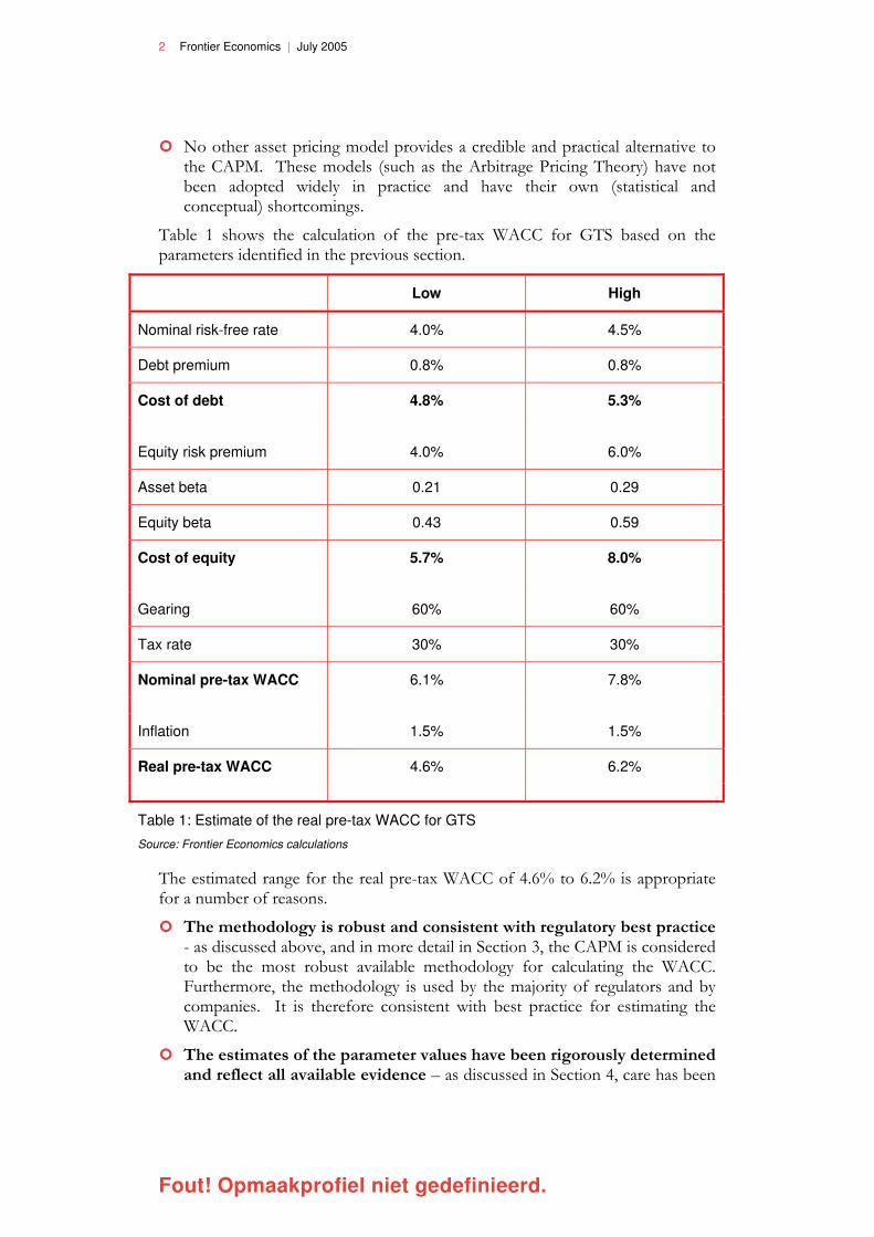
Table 1 shows the calculation of the pre-tax WACC for GTS based on the parameters identified in the previous section.
Low High
Nominal risk-free rate 4.0% 4.5%
Debt premium 0.8% 0.8%
Cost of debt 4.8% 5.3%
Equity risk premium 4.0% 6.0%
Asset beta 0.21 0.29
Equity beta 0.43 0.59
Cost of equity 5.7% 8.0%
Gearing 60% 60%
Tax rate 30% 30%
Nominal pre-tax WACC 6.1% 7.8%
Inflation 1.5% 1.5%
Real pre-tax WACC 4.6% 6.2%
Table 1: Estimate of the real pre-tax WACC for GTS
Source: Frontier Economics calculations
The estimated range for the real pre-tax WACC of 4.6% to 6.2% is appropriate for a number of reasons.
… The methodology is robust and consistent with regulatory best practice - as discussed above, and in more detail in Section 3, the CAPM is considered to be the most robust available methodology for calculating the WACC. Furthermore, the methodology is used by the majority of regulators and by companies. It is therefore consistent with best practice for estimating the WACC.
… The estimates of the parameter values have been rigorously determined and reflect all available evidence – as discussed in Section 4, care has been

3 Frontier Economics | July 2005
Fout! Opmaakprofiel niet gedefinieerd.
taken to ensure that the estimates for each of the parameter values in the WACC formula are consistent with available financial evidence and are consistent with both financial theory and regulatory precedence:
• the value of the nominal risk-free rate is consistent with the average yield on 10-year government debt in the Netherlands over a horizon of up to five years;
• the value of the debt premium is based on an assessment of comparator data for similar companies with an investment grade credit rating;
• the estimate of the equity risk premium is consistent with international evidence on the ERP, survey evidence and evidence from models of ERP expectations;
• the asset beta value is based on an in-depth analysis of comparator data for similar companies – with a range of methodologies for estimating betas assessed – and incorporates a Bayesian adjustment and conversion from equity betas using the standard Modigliani-Miller formula;
• the equity beta is directly converted from the asset beta estimate using the assumed gearing level and the level is consistent with the low risk regulatory regime that DTe expects to apply to GTS;
• the gearing level is consistent with the levels assumed by other regulators and with the gearing levels of similar companies;
• the tax rate is equal to the corporation tax rate that GTS is currently expected to face during the regulatory period; and
• the inflation rate is consistent with the medium term inflation forecast of the CPB.


5 Frontier Economics | July 2005
Fout! Opmaakprofiel niet gedefinieerd.
1 Introduction
This report provides an estimate of the appropriate cost of capital range to apply to GTS, the Dutch gas transportation network, for the next four year regulatory period (2006 to 2009). The report assesses the appropriate methodologies for deriving the cost of capital and estimates the key parameters in the calculation. The estimates are based on up-to-date financial market data and information on comparator firms.
The report is structured as follows.
… Section 2 summarises the regulatory regime that DTe expects to apply to GTS for the period 2006 to 2009.
… Section 3 assesses the main methodological issues involved in estimating the cost of capital.
… Section 4 details the estimation of the key parameters in the cost of capital calculation.
… Section 5 provides the calculation of the overall weighted average cost of capital for GTS.


7 Frontier Economics | July 2005
Fout! Opmaakprofiel niet gedefinieerd.
2 The regulatory regime for GTS
2.1 INTRODUCTION
The regulatory regime that will be applied by DTe to GTS in the period 2006 to 2009 is a relevant factor in determining the appropriate cost of capital. The regulatory regime has an affect on the level of risk faced by the regulated business and this feeds through into the cost of finance. An assessment of the regulatory regime is also useful in identifying appropriate comparator businesses used in the estimation of the cost of capital parameters, in particular the appropriate value for Beta. We describe the regulatory regime that is proposed for GTS here but note that the description is preliminary as the final details have not been finalised by DTe at this stage.
2.2 DESCRIPTION OF GTS
GTS is the national gas transportation company in the Netherlands. As of January 1st 2005, it is 100% owned by the State and the regulated network business is entirely separate from Gasunie’s other activities.
The regulated business includes gas transportation, quality conversion (50% in transport tariffs and 50% in quality conversion tariffs) and balancing services. While these activities have separate tariffs the regulatory control of the transportation activities applies to the revenues from all of them. Other GTS activities that are not included in the transportation regulatory control are flexibility services and responsibilities relating to GTS’s role as supplier of last resort and as the guarantor of security of supply in the event of extreme cold weather. These responsibilities are regulated separately by DTe.
2.3 DESCRIPTION OF THE REGULATORY REGIME
DTe is currently finalising the methodology that will be used to regulate GTS’s transportation tariffs from 2006 and, hence, this description should be treated as preliminary. The general framework is expected to be a cost plus regime, where allowed revenues for the regulatory period will reflect estimated actual costs in 2005. Estimated costs will be determined as operating expenditure, plus depreciation plus the return on the regulatory asset base (cost of capital times the regulatory asset base). Any surplus profits above actual costs will be removed through the use of an annual, nominal, X-factor. It has yet to be decided whether the control will be placed on revenues or on a tariff basket. The form of the control will affect risk to some extent, through the impact of volume growth on revenue volatility.
It is expected that annual required investments will be consistent with historical actual levels in the future. Furthermore, DTe is currently considering a proposal from GTS that new investments should only be undertaken if a sufficient number of market participants want to engage in a longer term contract with GTS. If implemented, such an approach may reduce long-term investment risks.
8 Frontier Economics | July 2005
Fout! Opmaakprofiel niet gedefinieerd.
It is also expected that, as with the regional networks, all operating expenditure will be treated as controllable and there will be no pass-through mechanism for any specific expenditure items.
Finally, DTe anticipates that the real WACC will be adjusted at the end of the period (i.e. at the review for the next price control) for differences between actual and forecast inflation, and for differences between actual and expected statutory tax rates. Such an approach would lower GTS’s exposure to inflation and tax risks.
A four year control will be applied in the first instance, allowing for the company and other stakeholders to adapt to the new regime. In time this may be extended to a maximum of five years.
In future regulatory periods it is expected that a system similar to that used for TenneT will be applied. In particular, revenues will be related to efficient costs rather than actual costs – where efficient costs will be determined on the basis of an international benchmarking exercise. It is expected that the benchmarking analysis will get underway during the second regulatory period.
In the short-term however the regime is expected to be based on actual costs (i.e. benchmarking will not affect the control set for the first and second periods) and as such is expected to be a low-powered incentive regime and a reasonably low risk regime.

9 Frontier Economics | July 2005
Fout! Opmaakprofiel niet gedefinieerd.
3 Methodology for calculating the cost of capital
3.1 INTRODUCTION
In this section we evaluate the appropriate methodology available for calculating the cost of capital. The evaluation is based on a wide range of evidence, including:
• decisions by other regulators;
• corporate finance theory; and
• the practical application of finance theory by corporations and finance practitioners.
It is recommended that the cost of capital for GTS is estimated using a weighted average cost of capital (WACC), with the cost of equity calculated using the Capital Asset Pricing Model (CAPM). This approach will base the estimate of the cost of capital on a measure of the opportunity cost of funds. The main parameters in the calculation will therefore be estimated from financial market data and from information on comparator companies with similar characteristics to GTS.
There are a number of reasons why the CAPM is considered the preferred methodology.
… The WACC reflects the two main types of finance used to fund investment: debt and equity.
… The CAPM approach to estimating the cost of equity is well established, solidly grounded in finance theory and straightforward to apply in practice.
… The WACC-CAPM methodology is the most common choice of regulators and private companies.
… Basing the estimate of the cost of capital on financial market data for comparator companies, rather than data on the company’s current cost of finance, has a number of advantages2. First, it should ensure that the cost of capital is set at an efficient level that reflects the underlying market cost of raising finance. Second, the use of external benchmarks should provide greater consistency in the estimates of the cost of capital over time.
… In practice the application of the CAPM approach requires rigorous estimation of the main parameters. In particular, there can be uncertainty regarding the appropriate values for the equity risk premium and the Beta value. This issue is best dealt with through careful choice of the methodology for estimating each of the WACC parameters (see Section 4). It is also
2 These advantages are in addition to the practical reality that market data is not available for GTS as it is a publicly owned company.
10 Frontier Economics | July 2005
Fout! Opmaakprofiel niet gedefinieerd.
important to note that empirical studies have shown that the CAPM methodology does not explain all of the difference in equity returns between companies. Our preferred methodology reflects these factors in three ways:
• first, recognising the uncertainty in the estimates through identifying an appropriate range for some of the parameters and therefore a range for the overall WACC;
• second, by cross-checking, where possible, the results of the CAPM approach against other evidence on the cost of capital; and
• third, by allowing the parameters to be estimated in a conservative way or by taking these factors into account when choosing appropriate parameter values.
… Nevertheless, there is no other asset pricing model that provides a credible and practical alternative to the CAPM. These models (such as the Arbitrage Pricing Theory) have not been adopted widely in practice and have their own (statistical and conceptual) shortcomings.
3.2 WACC FORMULA
When assessing the required capital costs for GTS, a key issue for DTe is to estimate what that opportunity cost of capital is. This should take into account the two principal sources of investment capital – debt and equity.
Consequently, the formula for the (post-tax) weighted average cost of capital is a weighted average of the two:
WACC = g x rd + (1-g) x re
Where:
rd is the cost of debt
re is the cost of equity
g is the proportion of finance that is debt i.e. g equals (debt/[debt + equity]).
The formula for the pre-tax WACC is
WACCpre-tax = g x rd + [(1-g) x re]/(1-T)
Where T is the corporate tax rate.
The WACC value to be applied to GTS will be a pre-tax real cost of capital. As the WACC is applied to a real value for the regulatory asset base, a real WACC is considered appropriate. Similarly, a pre-tax WACC is appropriate as it is expected that tax will not be included as a separate cost element elsewhere in the calculation of GTS’s total costs. Section 4 details the estimation of all the parameters in the WACC calculation.

11 Frontier Economics | July 2005
Fout! Opmaakprofiel niet gedefinieerd.
3.3 METHODOLOGIES FOR WACC DETERMINATION
The methodological basis for the determination of the WACC is rooted in modern finance theory, and the asset pricing models that have been developed as that theory has evolved.
The choice of appropriate methodology should take account of the following factors:
• the theoretical foundations of the methodology;
• ease of practical application;
• regulatory precedent; and
• DTe’s objective of maintaining a transparent regulatory regime.
The choice of methodology is not itself influenced by the characteristics of GTS per se, although the approach to evaluating each of the parameters of the WACC formula will take account of company characteristics and the nature of the regulatory regime. In other words, the methodology is chosen on the basis of ‘best practice’ principles rather than sector- or company-specific issues.
3.3.1 CAPM
Methodology
The most well-known, and most widely-used, asset pricing model is the CAPM. The CAPM relies on the assumption of a rational investor, who creates an optimal portfolio from different assets taken in certain proportions, so that the resulting combination offers the best possible trade-off between risk and return. Although the appetite for risk is different for each investor, the CAPM makes a general assumption that all investors are risk-averse: in other words, an investor will take on more risk only if compensated with a higher return.
The CAPM makes some other important simplifying assumptions, which allow the cost of equity for a company to be determined using a simple formula. The most important of these assumptions states that all existing information is freely and instantly available to all investors, and they all make the same conclusions based on this information in regard to the expected returns and risks of securities. In other words, all investors are assumed to have the same market perceptions.
A key implication of this assumption, and a well known result of the CAPM, is that all investors will have a portfolio that includes all available risky assets and the proportion of risky assets held will be the same for all investors. Specifically, each investor will hold a riskless asset and a portfolio of risky assets. The proportion invested in the riskless asset will depend, among other factors, on the risk aversion of the investor. However, once the amount to be invested in the portfolio of risky assets is determined, the investor will choose to hold all risky
12 Frontier Economics | July 2005
Fout! Opmaakprofiel niet gedefinieerd.
assets in his portfolio and all investors will buy the same risky assets in the same proportions. This optimal portfolio of risky assets is called the market portfolio.
The CAPM shows3 that the appropriate cost of equity is calculated as follows:
re = rf + ˚ x (rm - rf)
Where:
rf is the risk-free rate;
˚ (Beta) is the measure of relative (or non-diversifiable) risk of the company or industry; and
rm is the expected return on the market. The difference between the market return and the risk-free rate is known as the equity risk premium (ERP)4.
Non-diversifiable, or systematic risk, measured by ˚, is part of the total risk of the company that is related to the market: when the return on the market moves up or down, the return on the company’s equity will move by more than the
market return (if ˚ is greater than 1 in absolute terms) or less than the market
return (if ˚ is less than 1 in absolute terms).
Each company also has unique, or company-specific, risk that is not related to the overall market risk. However, in a sufficiently large portfolio this company-specific risk is close to zero: as some securities go down as a result of an unexpected bad news, others go up as a result of an unexpected good news, and on average any such fluctuations cancel out. As a result, unique risk does not enter the formula for calculating a company’s equity risk premium. Investors get rewarded only for bearing the systematic part of the company risk, because they can and are expected to diversify away the unique risk.
Usage by regulators and companies
CAPM’s clear theoretical foundations and simplicity make it by far the most widely used tool for practical cost of capital estimation. For example, according to the recent CEPA study for DTe5, in 12 out of the 13 recent regulatory cases for which information is available, the regulators used CAPM to estimate the cost of equity. In one case (US), a regulator used the Dividend Growth Model (DGM). In three cases where the CAPM was used as the primary method, it was also supplemented by other approaches: DGM (in two cases) and a range of direct market evidence (in one case).
3 For a detailed derivation see, for example, Sharpe, Alexander and Bailey, Investments, Prentice Hall: New Jersey, 6th edition, 1999.
4 This is sometimes referred to in the literature as the Market Risk Premium (MRP).
5 Cambridge Economic Policy Associates Ltd, An International Comparison of the Regulated Cost of Capital, February 2005.

13 Frontier Economics | July 2005
Fout! Opmaakprofiel niet gedefinieerd.
International surveys of Chief Financial Officers (CFOs) of private companies also show that the CAPM is the most widely used tool for estimating the cost of equity. In the US, over 70% of respondents reported using the CAPM (Figure 1). In Europe, the share of respondents who use CAPM was around 50%, while the second and third most popular methods were the use of average historical returns and the use of some version of a multi-factor CAPM6.
Figure 1: Methods used to estimate the cost of equity - survey of 400 US CFOs
Source: Graham and Harvey, The theory and practice of corporate finance: evidence from the field, Journal of Financial Economics, May 2001
Assessment of the CAPM model
The CAPM approach has a number of important strengths that explains its popularity.
… The model is derived from clear theoretical foundations. The concept that equity investors will hold a portfolio of assets and will be concerned with the impact of an individual investment on the portfolio as a whole is a very powerful one.
… The CAPM formulation is transparent and easy to implement. The difference in required return between different activities is captured in a single parameter – the Beta. In other asset pricing models differences in the riskiness of activities may be reflected in a number of different parameters.
6 Brounen, Dirk, de Jong, Abe, and Koedijk, Kees, Corporate Finance in Europe – Confronting Theory with Practice, Working Paper, Erasmus Research Institute of Management (ERIM), Erasmus Universiteit Rotterdam, Jan. 2004.
Method used to estimate cost of equity - % always or
almost always
0%
10%
20%
30%
40%
50%
60%
70%
80%
CAPM Historicreturns on
equity
CAPM withextra riskfactors
DGM What investorstell us
Regulatorydecisions

14 Frontier Economics | July 2005
Fout! Opmaakprofiel niet gedefinieerd.
… The results are relatively easy to interpret. This is because, under the CAPM, the Beta can be considered to be independent of the performance of the company under consideration. Other models are driven by factors, such as the market / book ratio, which will depend on the performance of the company. In these cases it is more difficult to interpret the evidence in terms of setting a forward-looking cost of capital.
… The CAPM approach is well-established. In particular, it has been consistently used by regulators and corporations as the principal methodology for estimating the cost of equity.
There are a number of weaknesses with the CAPM framework, though these weaknesses are often present with alternative models as well.
… One limitation of the CAPM is the assumption that the cost of equity depends only on the degree of non-diversifiable risk in a given stock. Clearly, other factors may play a role as well, and there is a body of evidence suggesting that investors care about more factors than just the non-diversifiable risk. There is substantial ongoing research trying to incorporate such other factors into applied models. Some of the well-known advances in this area are the multi-factor extensions of the CAPM, which assume that the cost of equity depends on several factors rather than just one7. However, all such models have a number of statistical problems associated with them, they are still in the development phase, and no single methodology has been commonly accepted as a practical tool. The models are therefore not considered to be credible alternatives to the CAPM.
… Recent research suggests that a carefully specified “conditional” CAPM – i.e., one in which the parameters vary over time – usually performs better than a non-linear model. But this methodology is also only at the development stage8.
… An issue with the practical application of the CAPM is uncertainty over forward-looking estimates, which have to be proxied by historical data. It is appropriate to take account of this uncertainty when deciding how to value the parameters – as discussed in Section 4 – rather than simply choosing to not use CAPM because of this potential shortcoming. This uncertainty will apply equally to other asset pricing models.
One particular issue is that GTS is publicly owned with, on the face of it, non-diversified shareholders. This raises the question as to whether the CAPM is still an appropriate approach in this case. In practice this issue should not invalidate the use of CAPM. The ownership structure of GTS means that it is not possible to observe the cost of equity using market data for GTS. However this can be overcome by using market data on comparator companies.
7 A famous example is the Fama and French multi-factor model, where the two additional factors are company size and book-to-market ratio. Another group of alternative models is based on the Arbitrage Price Theory (APT), which is discussed below.
8 Wright, Stephen, Robin Mason and David Miles, A Study into Certain Aspects of the Cost of Capital for Regulated Utilities in the U.K. On behalf of Smithers & Co Ltd, 2003.

15 Frontier Economics | July 2005
Fout! Opmaakprofiel niet gedefinieerd.
The second issue is whether the ownership structure of GTS should be taken into account in estimating the appropriate cost of capital. There are two main reasons why the ownership structure should not affect the assessment of the cost of capital.
… First, ownership by the public sector does not necessarily imply that the investor is not diversified. A government or municipality shareholder will be involved in / exposed to many other sectors of the economy. As a result, a public sector shareholder may have a comparable degree of diversification to a private sector shareholder.
… Second, to the extent that a diversified investor has the lowest cost of capital for a particular activity, a diversified investor will set the efficient cost of finance. Regulators will want to take account of efficient costs (financing and other) in setting prices to ensure that prices are set at the right level – in terms of encouraging efficient consumption and investment decisions. In this regard, there are a number of examples where regulators have applied the CAPM approach to utilities owned by the government or by local municipalities9.
3.3.2 Other asset pricing models
The theoretical finance literature contains numerous alternative asset pricing models for estimating the cost of equity. These include arbitrage pricing theory (APT) and developments of the CAPM (including consumption-CAPM and multi-factor models). To date, corporations or regulators have not adopted these models to any degree. These models may have performed better in predictive tests than the standard CAPM but they lack the conceptual coherence of the CAPM framework. We therefore think it is inappropriate to use these alternative models to estimate the cost of capital for GTS.
Arbitrage Pricing Theory
One of these alternative approaches is the Arbitrage Pricing Theory (APT). While the CAPM starts with an explicit model of investor behaviour, the APT rests on a more primitive assumption: that there should be no arbitrage opportunities in an economy. In addition, the APT assumes that the payoff of a risky asset is generated by a certain number of factors, all of which influence the total payoff in a linear way.
The APT uses these two assumptions to derive a prediction about expected rates of return in risky assets. When the number of factors is just one, and that factor is the market portfolio, the APT prediction reduces to the CAPM equation.
The main difficulty with the APT lies in its empirical application. The APT itself does not identify which are relevant factors or how many factors there will be.
9 In addition to DTe’s decisions for TenneT and the regional networks, other examples of regulators using the CAPM for publicly owned companies include CER’s regulation of the gas transmission company in Ireland, the CAA’s regulation of Manchester Airport and E-Control’s regulation of the gas transportation companies in Austria..

16 Frontier Economics | July 2005
Fout! Opmaakprofiel niet gedefinieerd.
As a result there has been a lengthy academic debate regarding the identification of the appropriate factors. This partly explains why the APT has failed to gain popularity with regulators or corporations as a practical method for assessing the cost of capital.
Extensions of CAPM
To take account of the possibility that asset returns are influenced by more than one factor, a number of straightforward multi-factor extensions of the basic CAPM theory have been developed, such as the consumption CAPM (CCAPM) and the intertemporal CAPM (ICAPM). In the CCAPM, the additional factor influencing the cost of equity is assumed to be the aggregate consumption (or anything correlated with it). In the ICAPM, it is assumed that there exists a limited number of “state variables” (e.g., technology, employment, income, the weather) that are correlated with assets’ rates of return.
An example of a multi-factor model developed from an empirical analysis is the three-factor model developed by Fama and French which includes market size and book-to-market ratio as additional explanatory variables. The book-to-marker ratio may have been a factor in explaining historic US equity returns, however, it has not performed as well empirically for other markets. Furthermore, it does not provide any information for a regulator setting the rate of return for a utility.
Although plausible conceptually, multi-factor models have failed to establish themselves, which explains why they have not gained any significant popularity for practical cost of capital estimation compared to the CAPM.
3.3.3 Dividend Growth Model
The most commonly used alternative approach to estimating the cost of equity is the Dividend Growth Model (DGM)10. The DGM is based on the premise (the dividend discount model) that the value of a company’s equity is the net present value of the future stream of dividends per share.
This concept for valuing equity can be converted into a model of the cost of equity by assuming that the future growth rate of dividends is a constant. Under this assumption, and by rearranging the formula, the DGM is derived:
re(nominal) = dividend yield per share + nominal expected dividend growth rate
The advantage of the DGM (like CAPM) is that it is simple to understand and to implement. On the downside, the dividend per share growth rate is usually based on analyst expectations, and there is large uncertainty about this parameter. As a result, the out-turn cost of equity estimate that the model delivers is highly sensitive to this assumed growth in dividends paid.
10 The DGM is more widely used by regulators in the US. For example, this model was used in 6 out of 8 US energy decisions cited in the report International comparison of WACC decisions, NECG, September 2003.

17 Frontier Economics | July 2005
Fout! Opmaakprofiel niet gedefinieerd.
Dividend forecasts are often available for a period of up to five years but assumptions need to be made regarding investor’s expectations for dividend growth beyond that point. Alternative scenarios for dividend growth can produce a wide range for the estimated cost of equity.
One option that is often employed is to use the DGM to estimate the cost of equity for the market as a whole, as opposed to a particular equity. The advantage of this is that there is less uncertainty regarding the future growth rate of dividends for the market than there is for dividend growth for an individual company. The estimate of the cost of equity can then be used to estimate the equity risk premium in the CAPM model. This approach has been used in a number of studies.
Our view is that the DGM is not an appropriate approach for estimating the cost of equity for GTS due to the uncertainty surrounding future dividend growth. However, it is a useful model for cross-checking the view of the overall cost of equity for the market and we have benchmarked our findings using this approach (see Section 4.4.1).
3.3.4 Other evidence on expected investment returns
A further source of information is evidence from market investors. For the cost of equity, additional evidence could come in the form of data from market transactions (flotations or equity issues) or from surveys of investor expectations. If such evidence is available it can serve as a useful crosscheck to the core analysis.
There are a number of advantages and disadvantages to evidence of this type. The main advantages are that:
• the information reflects the direct views of the financial community or is based on data from recent financial transactions – as a result it should measure the actual costs of raising finance;
• the evidence is up-to-date, based on recent transactions or current survey evidence; and
• the information is, in some cases, transparent - which reduces the scope for disagreement between the regulator and the regulated companies.
However, the disadvantages of this evidence are that:
• the evidence from surveys may be biased, reflecting the vested interests of the participants;
• evidence from market transactions may be limited / infrequent – the evidence may also relate to all activities undertaken by the floated company rather than the specific regulated activities of interest; and
• interpreting some of the evidence may require analysis and assumptions –for example, the cost of equity could be estimated but only by making assumptions about future cashflows.

18 Frontier Economics | July 2005
Fout! Opmaakprofiel niet gedefinieerd.
In 2000 the UK Competition Commission considered the relevance of survey evidence in establishing the appropriate ERP. The Commission was cautious about attaching too much weight to this evidence:
“The survey and other evidence discussed above leads to quite a wide range of figures. This evidence may be subject to biases which are difficult to quantify and assess: fund managers may have the incentive to quote lower figures to make their achievements look better but, on the other hand, if they know the use made of the evidence, they have the incentive to quote higher figures since they benefit directly from a higher cost of capital for regulated companies. Probably for this latter reason, the evidence tends not to be derived from rigorously structured surveys.”11
While it would not be appropriate to rely solely on survey information, evidence such as this could form part of the evidence base. In the case of regulated energy companies in the Netherlands, the absence of quoted companies indicates that investors’ survey are unlikely to feature in the estimation of the cost of capital.
3.3.5 Summary on alternative approaches to the cost of equity
Alternative asset pricing models have been developed to address the conceptual and empirical weaknesses with the CAPM framework. None of these models have established themselves as a credible alternative to the CAPM and, hence, the CAPM remains the principal method for estimating the cost of equity. Nevertheless, the information provided by other models – notably the DGM - and other evidence on required equity returns can provide useful benchmarks to cross-check the results of the CAPM calculation.
11 Competition Commission, Sutton and East Surrey Water plc, September 2000, para 8.28.

19 Frontier Economics | July 2005
Fout! Opmaakprofiel niet gedefinieerd.
4 Parameters of the WACC calculation
4.1 INTRODUCTION
This section of the report estimates the parameters of the WACC calculation for GTS – principally using the CAPM approach. The section considers the preferred methods for estimating these parameters as well as calculating the appropriate values for GTS.
4.2 FORMULA FOR THE WACC
As discussed earlier, it is appropriate to use a real pre-tax WACC when setting the revenue cap for GTS.
The formula for the real (post-tax) weighted average cost of capital (WACC) is a weighted average of the cost of equity and the cost of debt:
WACCpost-tax = g x rd + (1-g) x re
Where:
rd is the real cost of debt
re is the real cost of equity
g is the proportion of finance that is debt i.e. g equals (debt/[debt + equity]).
The formula for the real pre-tax WACC is
WACCpre-tax = g x rd + [(1-g) x re]/(1-T)
Where T is the corporate tax rate.12
4.3 COST OF DEBT
The cost of debt is typically expressed as the sum of the risk-free rate and debt premium. This aids comparisons across companies, countries and time. The risk-free rate is also a key parameter in the cost of equity calculation.
4.3.1 Estimating the nominal risk-free rate
The risk-free rate depends on market conditions in the economy and is not therefore influenced by any company specific factors. As a result, although the appropriate value for the risk-free rate may vary over time the calculation will not vary from industry to industry in the Netherlands.
12 The third definition of the WACC is post-tax net of tax shield on debt. The definition of this is:
WACCpost-tax = [(g x rd)x(1-T)] + (1-g) x re

20 Frontier Economics | July 2005
Fout! Opmaakprofiel niet gedefinieerd.
It is possible to estimate the risk-free rate of return from market data on interest rates and government bond yields. For mature and well-developed economies the yield on government debt is seen as a good proxy for the true risk-free rate13.
The main issues to consider in developing an estimate of the risk-free rate are:
• the appropriate maturity of debt; and
• whether to use current rates or long-term averages.
Maturity of debt
Interest rates will typically rise with the maturity of the debt. This is illustrated in Figure 2, which shows the yields on Netherlands Government loans between 1994 and 2003. It shows that the interest rate rises with the maturity of the debt (this is known as the term structure of interest rates).
Figure 2: Yields on government loans
Source: DNB, Central Bank of Netherlands
Over this period for the Netherlands, each additional year of maturity adds 10 basis points (0.1%) to the interest rate.
In deciding the appropriate maturity to use in estimating the risk-free rate, there are a number of factors to take into account.
13 The probability of default on this debt is extremely low. As a result the yield provides a reasonable estimate of the concept underlying the risk-free rate – the return that investors require to defer consumption from one period to the next.
0.0
1.0
2.0
3.0
4.0
5.0
6.0
7.0
8.0
9.0
Jan-
94
Jul-9
4
Jan-
95
Jul-9
5
Jan-
96
Jul-9
6
Jan-
97
Jul-9
7
Jan-
98
Jul-9
8
Jan-
99
Jul-9
9
Jan-
00
Jul-0
0
Jan-
01
Jul-0
1
Jan-
02
Jul-0
2
Jan-
03
Jul-0
3
%
3 - 5 years 5 - 8 years
10 years

21 Frontier Economics | July 2005
Fout! Opmaakprofiel niet gedefinieerd.
… Short-term interest rates are a better proxy for the true risk-free rate. Part of the explanation for the term structure of interest rates is that long-term government debt is more risky than short-term government debt. Although the risk of default on long-term government debt is still very low, it will be higher for long-term debt than short-term debt and this will be reflected in the interest rate. Furthermore, longer-term debt will also be exposed to greater inflation risk (this is discussed further below). As a result, the short-term interest rate will tend to be a better approximation of the true risk-free rate.
… Consistency with the equity risk premium estimate. The ERP is calculated as the return on equities in excess of the return on government debt (see section below). The choice of maturity used to estimate the risk-free rate should be consistent with the maturity used to calculate the ERP.
… Short-term interest rates are more volatile. One advantage of using longer-term interest rates is that short-term interest rates are typically more volatile than longer-term interest rates. Short-term rates respond more to changes in government policy and to changes in inflation expectations. For a regulator that is looking to estimate a risk-free rate that will be appropriate for a number of years (for example, price control period of 3 to 5 years) there is an advantage in using a more stable measure of interest rates.
… Medium-term maturities are more consistent with corporate debt financing patterns. A further factor in favour of focusing on longer-term interest rates is that it should be more representative of the financing behaviour of companies. Companies will typically have a debt portfolio with a mix of maturities, but it would not be unusual for a utility company to have an average debt maturity of between 5 and 10 years.
In forming a view of the appropriate risk-free rate we have considered evidence on yields with maturity of 5 years and 10 years. The evidence in the CEPA report14 shows that European regulators typically use a 10-year maturity for assessing the risk-free rate.
Time period for assessing data
The majority of regulators base the assessment of the risk-free rate upon current market data. Typically estimates are based on the trends over a recent period rather than market rates on a given day. The period over which interest rates are assessed may vary from two or three months to a number of years. The reasons for taking an average over a reasonable period are:
• market interest rates may be relatively volatile over short-periods of time;
• to the extent that short-term changes in interest rates reflect underlying changes in investors’ expectations these changes may not be reflected in the available data on the other components of the cost of capital (ERP,
14 Cambridge Economic Policy Associates Ltd, An International Comparison of the Regulated Cost of Capital, February 2005.

22 Frontier Economics | July 2005
Fout! Opmaakprofiel niet gedefinieerd.
Beta and debt premium) – reflecting these changes only in the risk-free rate may not be appropriate; and
• in a regulatory process, there is an advantage in building in a degree of certainty and stability in the calculations during the course of consultations and draft price controls.
A period around two years provides, in most cases, a sensible balance across these factors. Data from the Central Bank of the Netherlands indicates that the average yield on 10-year government debt over this period has been 4.0%.
Time period (to June 2005)
Yield on 10 year maturity – average
over period
6 months 3.5%
1 year 3.7%
2 year 4.0%
3 year 4.1%
5 year 4.5%
Table 2: Yield on Netherlands Government debt
Source: Central Bank of Netherlands
Table 2 shows average yield over periods from six months to five years, and reveals that the government debt yield is currently below the five year average. Given the current low level of yields, it would be prudent to take account of the data over a longer period in assessing the appropriate forward-looking risk-free rate. Over the past five years the average yield has been 4.5%. The average yield over a two year period and a five year period provides a sensible range for the nominal risk-free rate – 4.0% to 4.5%.
Summary on the nominal risk-free rate
The risk-free rate is used in the estimation of the cost of equity and the cost of debt. Care needs to be taken to ensure that the appropriate debt maturity, time period and inflation adjustment (see below) are used to estimate the risk-free rate.
A range of 4.0% to 4.5% for the nominal risk-free is appropriate.
4.3.2 Estimating the debt premium
The second element of the cost of debt is the debt premium – the additional return expected by debt investors to invest in corporate debt compared to government debt.
Companies have a number of options, including:
• banks loans;
• syndicated loans;
• finance leases;

23 Frontier Economics | July 2005
Fout! Opmaakprofiel niet gedefinieerd.
• commercial paper; and
• corporate bonds.
Public domain data is typically only available for quoted corporate bonds15 and these are the primary source of data used to estimate the debt premium. The debt premium is therefore measured as the redemption yield on corporate debt minus the risk-free rate. The government bond used to estimate the risk-free rate should be of the same maturity as the corporate bond16.
Our approach to estimating the appropriate debt premium for GTS is to analyse data on corporate bond premium for a range of comparator companies that are similar to GTS. In general the use of comparator data is sensible because it provides a larger sample of data and allows an assessment of the debt premium under different credit ratings and levels of gearing. In the case of GTS the absence of quoted data on the company’s debt further underlies the importance of comparator data.
Choosing comparators
The process of identifying comparators is more straightforward in the case of the debt premium than is the case with Beta (see below). There are two reasons for this:
• the range of factors that determine the debt premium is relatively small; and
• more importantly, the combined impact of these factors is captured in a single measure – the credit rating.
Companies that issue quoted debt will seek a credit rating from one or more of the established credit rating agencies (e.g. Standard & Poors, Moodys). The credit rating provides a composite and forward-looking measure of the risk of default of the debt. The rating agency’s assessment will take into account factors such as:
• level of gearing;
• volatility of cash-flows;
• industry characteristics; and
• form of regulation.
15 A regulator could ask companies to provide information on bank loans and other sources of debt finance. However, even then a key advantage of quoted corporate debt is that the yield on the debt will be updated to reflect current investor expectations.
16 In other words, the debt premium on a 20 year corporate bond should be estimated with reference to the yield on a 20 year government bond; a 10 year corporate bond compared to a 10 year government bond; and so on.

24 Frontier Economics | July 2005
Fout! Opmaakprofiel niet gedefinieerd.
For a group of similar industries there will be a strong correlation between the credit rating and the debt premium. As a result, the possible set of comparators can include all companies with quoted debt that operate within similar industries.
Figure 3: Debt premium (basis points) on US utility bonds
Source: Bondsonline
Figure 3 shows an example of how the debt premium increases as the credit rating declines. Debt with a rating of BBB- or higher is considered to be investment grade. The data shows that there is a significant increase in the debt premium once the quality of debt moves below investment grade.
Figure 4 shows how the debt premium has fluctuated over time, based on data for European corporate bonds. The fluctuations in debt premium are more pronounced for the lower credit rating, with the premium on BBB showing greater volatility than the premium for AA or A rated bonds.
Figure 4: Debt premium on European corporate bonds
Source: Ecowin
0.0%
0.5%
1.0%
1.5%
2.0%
2.5%
3.0%
Jan-
99
May
-99
Sep-9
9
Jan-
00
May
-00
Sep-0
0
Jan-
01
May
-01
Sep-0
1
Jan-
02
May
-02
Sep-0
2
Jan-
03
May
-03
Sep-0
3
Jan-
04
May
-04
Sep-0
4
BBB A
AA
Rating 10 year maturity
AAA 15
AA+ 18
AA 29
AA- 43
A+ 58
A 60
A- 62
BBB+ 78
BBB 103
BBB- 115
BB+ 275

25 Frontier Economics | July 2005
Fout! Opmaakprofiel niet gedefinieerd.
Gearing will be an important determinant of credit rating. As gearing increases we would expect the credit rating to decline and the debt premium to increase. If the comparator data were based on companies with lower gearing and better credit ratings than that proposed for the WACC calculation for GTS then appropriate adjustments would need to be made. We discuss the level of gearing for GTS further below.
Evidence on the debt premium
The sample of comparators chosen to estimate the debt premium are shown in Table 3. The comparators are different to those used to estimate GTS’s Beta as data availability varies depending on whether we are looking for similar companies with quoted debt (as here) or similar companies with quoted shares (as for the Beta). In particular, not all companies that have quoted debt have quoted shares, and vice versa. Furthermore, the factors used to identify appropriate comparators are fewer and more generic in the case of the debt premium calculation and, hence, the need to take account of a wider range of factors when estimating the equity beta changed the set of appropriate comparators.
Company Maturity of bond – as at April 2005
Market gearing Credit rating – as at April 2005
Red Electrica (Spain) 8 years 49% AA-
Acea (Italy) 9 years 43% A+
Essent (Netherlands) 8 years N/a A+
Eneco (Netherlands) 5 years N/a A+
NGT (UK) 12 years 51% A
Scottish Power (UK) 12 years 36% A-
United Utilities (UK) 13 years 49% A-
Envestra (Canada) 10 years 72% BBB
Union Gas (Canada) 10 years N/a BBB
Table 3: Corporate bond sample
Source: Bloomberg
Table 3 also shows the maturity of debt and the current credit rating and market gearing. The comparators have been chosen to satisfy the following characteristics:
• companies that focus on energy networks;
• debt with a maturity of around 10 years; and
• credit ratings focussed around a ‘single A’ rating.

26 Frontier Economics | July 2005
Fout! Opmaakprofiel niet gedefinieerd.
A ‘single A’ rating represents an appropriate benchmark for default risk of GTS under the proposed gearing assumption of 60%. We consider the reasonableness of this gearing assumption below.
Figure 5 shows the debt premium for the sample of corporate bonds over the past two years. Since the beginning of 2004 the premium has varied between 40 basis points and 100 basis points – with, not surprisingly, a higher premium for the bonds with a lower credit rating.
Figure 5: Corporate bond spreads
Source: Bloomberg
We would propose a debt premium for GTS of 0.8% (80 basis points). This lies towards the top of the range identified in the analysis (i.e. the values since the beginning of 2004). The upper end of the range is considered appropriate for three reasons.
… First, the current levels of debt premium are relatively low by historic standards.
… Second, the debt premium results in the Figure above do not make any allowance for transaction costs associated with issuing debt. These costs will be relatively small when spread over the life of the debt. Using a value from towards the top of the identified range will make adequate allowance for such costs.
… Third, the data in Figure 4 above shows that the debt premium on A rated corporate bonds has averaged 0.75% over the past five years.
20
40
60
80
100
120
140
May
-03
Aug-0
3
Nov
-03
Feb-0
4
May
-04
Aug-0
4
Nov
-04
Feb-0
5
May
-05
Sp
rea
d,
po
ints
(1
00
pts
= 1
%)
Red Electrica AA- Acea A+ Eneco A+
Essent A+ NGT A Scottish Power A-
United Ut. A- Envestra BBB Union Gas BBB

27 Frontier Economics | July 2005
Fout! Opmaakprofiel niet gedefinieerd.
4.4 COST OF EQUITY
The principal methodology for estimating the cost of equity is the CAPM formulation. To re-cap the CAPM formula for the cost of equity is:
re = rf + ˚ x (rm - rf)
Where:
rf is the risk-free rate;
˚ is the equity Beta (the measure of non-diversifiable risk of the company); and
(rm - rf) is the equity risk premium (ERP)
The risk-free rate has been addressed in the previous section. The remainder of this section considers the estimation of the ERP and the Beta.
4.4.1 Equity risk premium
The nominal ERP is additional return, above the nominal risk-free rate, that investors expect for holding the portfolio of risky assets. Evidence on the ERP is available from a number of sources:
• data on historic ERP from a number of countries;
• models of ERP expectations; and
• survey evidence on ERP expectations.
In addition, it is sensible to benchmark the estimate of the overall cost of equity for the market (i.e. the risk-free rate plus the ERP, given that the market Beta is equal to one by definition) against other sources of information on the overall cost of equity (e.g. estimates derived from the Dividend Growth Model). For a given risk-free rate, this provides a test of the reasonableness and consistency of the ERP estimate.
International evidence on the historic ERP
There is a wealth of data available on the returns on equity relative to the returns on relatively risk-free assets such as Government bonds. Data on financial market returns are available for a range of countries and in many cases the dataset extends back over 100 years. These datasets are typically used as the starting point for the estimation of the ERP.
Arithmetic and geometric mean estimates from historic data
In estimating the cost of capital using the CAPM we are interested in the expected annual return on equities relative to bonds. In terms of historic data, the arithmetic mean is analogous to the expected annual return. Nevertheless, the issue of whether the historic ERP should be estimated using the arithmetic

28 Frontier Economics | July 2005
Fout! Opmaakprofiel niet gedefinieerd.
mean or the geometric mean17 has been the subject of much debate18. The main points in the argument are as follows:
• the arithmetic mean will be higher than the geometric mean (unless the returns are constant over time in which case the arithmetic and the geometric mean will be the same);
• if returns are uncorrelated over time then the arithmetic mean will be the appropriate basis for predicting future returns and therefore the correct benchmark for estimating the ERP; and
• however, there is evidence of some degree of mean reversion in returns over the medium-term19; in this case the observed arithmetic mean (measured over a short period e.g. annual data) may overstate the forward-looking ERP.
The Smithers report for the UK regulators concludes that it has no strong preference for either approach but cautions that one should be aware of the potentially significant differences between the two. The authors of the report note that there are plenty of influential academic economists expressing views in favour of using each method20.
In summary, there is concern that historic estimates based on annual arithmetic means will overstate the forward-looking ERP. As a result, it is sensible to take account of both arithmetic and geometric means in forming a view of the appropriate ERP.
Dimson, Marsh and Staunton
One of the most comprehensive analyses of historic ERP data is a dataset created by Dimson, Marsh and Staunton. This analysis covered 16 countries over the period 1900 to 2002.
Figure 6 shows the historic ERP based on an arithmetic mean calculation and a geometric mean calculation. It shows the results for the “world” index (the total for the 16 countries in the sample) and for the Netherlands. The ERP for this “world” index over the 103-year period was 3.8% as a geometric mean and 4.9%
17 The arithmetic mean is the simple average of the individual period (in this case annual) returns. The geometric mean of a sample of N periods is the Nth root of the compound return.
18 The Smithers report has a useful summary of the literature (p23 – p27).
19 This is illustrated by the evidence, from the Dimson, Marsh and Staunton analysis, that the 10 year arithmetic mean is consistently lower than the average annual arithmetic mean.
20 For example, Campbell and his various co-authors tend to prefer the geometric average, while Fama and French have, in different papers, applied the arithmetic average. Copeland at el. (2001) find, based on a review of several academic studies, that there appears to be significant long-term negative autocorrelation in historical stock returns, and so they are not independent. Based on this result, the authors believe that the true market risk premium lies between the arithmetic and geometric averages. Dimson, Marsh and Staunton (2002), in a paper that extends and updates their previous study of global evidence on the equity risk premium, argue that in the future volatility of stock market returns will be lower than it has been over the last century. They conclude that historical estimates of the risk premium based on the arithmetic average should be adjusted downward to take account of this change.

29 Frontier Economics | July 2005
Fout! Opmaakprofiel niet gedefinieerd.
as an annual arithmetic mean. The ERP for the Netherlands was 3.8% (geometric) and 5.9% (arithmetic).
Figure 6: International evidence on the ERP: 1900 to 2000
Source: Dimson, Marsh and Staunton, 2002, Global Investment Returns Yearbook (ABN AMRO/London Business School, 2003)
Other studies
The Dimson, Marsh and Staunton dataset is the most comprehensive in terms of the number of countries covered, but there are other studies of historical equity and bond returns.
… Ibbotson Associates publish an annual report – Stocks, Bonds, Bills and Inflation Yearbook – with data on US capital market returns. This dataset shows that, over the period 1926 to 2001, the realized arithmetic equity premium in the US was 7.0%.
… A study by Siegel21, analysed US data over a longer period (1802 to 1998) and concluded that the average premium of equities over bonds (on an arithmetic basis) was 4.7%.
21 Siegel J, The shrinking equity premium, Journal of Portfolio Management 26(1), 1999.
3.8% 3.8%
4.9%
5.9%
0%
1%
2%
3%
4%
5%
6%
7%
Geometric mean Arithmetic mean
World Netherlands

30 Frontier Economics | July 2005
Fout! Opmaakprofiel niet gedefinieerd.
Relevance of historical data
In assessing the relevance of the historical data there a number of factors that need to be considered.
… First, there is significant variation in equity returns and the confidence intervals around estimates based on dataset going back even 100 years are relatively wide.
… Second, the confidence intervals around the estimates can be reduced by taking even longer periods (e.g. the Siegel analysis). However, the narrower confidence interval has to be offset against the question as to whether data from the 19th century represents a good basis for estimating forward-looking equity returns.
There is also the question as to whether the forward-looking ERP for the Netherlands should be based primarily on evidence from the Netherlands or from international equity markets. Dimson, Marsh and Staunton consider that any variation across countries in historical returns does not imply that future expected returns will vary in a similar way across countries. The historic equity returns for an individual country will reflect the specific circumstances and relative economic performance of the country over that time period. They argue that on a forward-looking basis investors should not expect these differences to continue. As a result, in assessing future returns it is appropriate to consider the evidence from a range of countries (i.e. it is appropriate to use the ERP for the “world” index).
In the case of the Netherlands, the historic data on returns for the Netherlands equity market are similar for the average returns achieved by other major economies over the same period. This provides additional reassurance that these average returns of the “world” index provide a useful foundation for projecting future returns in the Netherlands.
The international evidence on historic ERP provides a range of values from around 4% to 7%. Our assessment indicates that a narrower range of 4.0% to 6.0% is appropriate. In reaching this view we have taken account of all the historic evidence but we have placed greater weight on the Dimson, Marsh and Staunton evidence for the world equity indices and Siegel’s very long-term analysis of the US data, and less weight on the Ibbotson evidence for the USA (which lies above this range). The reasons to place less weight on the evidence from the Ibbotson study are:
• the Ibbotson study has a shorter time period than the Sigel analysis and therefore there is a greater confidence interval surrounding the results;
• the US economy has performed strongly (relative to other economies) over the period covered by the Ibbotson study and therefore may overstate the forward-looking premium for world indices; and
• the Dimson, Marsh and Staunton analysis, by looking at returns for 16 economies, provides the largest evidence base for assessing forward-looking returns.
31 Frontier Economics | July 2005
Fout! Opmaakprofiel niet gedefinieerd.
Nevertheless, the uncertainty around the historical evidence on equity returns means that it is important to look at other sources of the evidence on the forward-looking ERP.
Other evidence on the ERP
There are a number of other sources of evidence on the ERP that can be used to supplement the historic data. The most important of these are: models that use additional variables to adjust the historic returns data; and survey evidence on investors’ expectations.
Models of adjusted historic returns or forward-looking estimates
Academic studies have modelled investors ex ante expectations of equity returns based on time series data of equity returns and other macro-economic variables. Examples of these studies include the following22.
… The Fama and French model (2001)23. The approach in this paper infers the desired equity return based on a formulation of the Dividend Growth Model (where the expected equity return is equal to the current dividend yield plus the expected dividend growth rate). Applying this approach to the US produces an estimate of the ERP of 3.6% (covering the period 1872 to 1999).
… Ibbotson and Chen (2001)24 apply a similar approach to Fama and French, using historical data on earnings growth and GDP per capita to proxy dividend growth. This analysis obtains estimates of the ERP for the USA of 5.9% and 6.2%.
… Cornell (1999)25 applied a version of the dividend growth model which based the assessment of future dividend growth on investment analysts’ projections for the first five years followed by a transition to the long-term nominal growth rate of the economy. Applying this approach to 1996 data he estimated a forward-looking ERP of 4.5%.
… Dimson, Marsh and Staunton (2003) assess the appropriate forward-looking risk premium based on adjustments to the historic evidence. The adjustments reflect views on equity market volatility going forward and long-term changes in capital market conditions. They conclude that the prospective arithmetic risk premium would be around 5%.
These studies generate a wide range of estimates for the ERP, though there are two main themes emerging from this evidence:
• first, these studies tend to produce estimates of the ERP below that suggested by the historic data; and
22 See The Market Equity Risk Premium, New Zealand Treasury, May 2005 for a summary of this evidence (http://www.treasury.govt.nz/release/super/tp-tmerp-may2005.pdf).
23 Fama, Eugene F. and French, Kenneth R., The Equity Premium (April 2001). EFMA 2001 Lugano Meetings; CRSP Working Paper No. 522.
24 Ibbotson and Chen, The supply of stock market returns, Ibbotson Associates, 2001.
25 Cornell B, The equity risk premium: The long-run future of the stock market, New York NY Wiley, 1999.

32 Frontier Economics | July 2005
Fout! Opmaakprofiel niet gedefinieerd.
• second, many of these studies are still consistent with a range of the ERP of 4% to 6%.
Survey evidence of ERP expectations
Various surveys of ERP expectations have been undertaken. These surveys have covered financial economists, company finance officers and investment analysts. A summary of this evidence is provided below in Table 4. ERP expectations from financial economists and company finance officers tend to be in line with the observed historic data while the expectations from investment analysts and fund managers tend to be lower. In general the majority of the survey evidence suggests that a range of 5-6% is appropriate for the ERP, although the evidence from banks and fund managers points to a lower value.
Evidence Description Value for ERP
Welch, 2000 Survey of over 100 financial economists - mainly US
6%
Welch, 2001 Update of survey of financial economists
5%
OXERA March 2000 survey of ERP used by UK companies
5%
Bruner et al (1998) US survey of corporations and financial analysts
Corporate users favour range 5% - 6%
UK financial institutions Views from investment banks and fund managers since 1997
Most estimates lie in range 2 - 4%
Table 4: Expectations for ERP
Sources:
Bruner R, Eades K, Harris R and Higgins R (1998), ‘Best practices in estimating the cost of capital: survey and synthesis’, Financial Practice and Education, Spring / Summer
The OXERA (2000) report and the evidence from UK financial institutions were cited by the UK Competition Commission in the report Vodafone, O2, Orange and T-Mobile: Reports on references under section 13 of the Telecommunications Act 1984 on the charges made by Vodafone, O2, Orange and T-Mobile for terminating calls from fixed and mobile networks, (2003, p190).
Welch, I., 2000, ‘Views of financial economists on the equity premium and other issues’, Journal of Business 73 (October): 501-37
Welch I (2001), The equity premium consensus forecast revisited, working paper, Yale School of Management
Our analysis indicates a range for the nominal ERP of 4% to 6%. The lower end of the range is consistent with the upper bound of the range suggested by survey evidence from UK financial institutions and the estimates of US ERP from academic models of ERP expectations. The upper end of the range is consistent with the international evidence on the arithmetic and geometric mean and other survey evidence on the ERP.
Using a value for the real risk-free rate of around 2.5% to 3.0% (see below) this gives an overall figure for the real cost of equity for the market of between 6.5% and 9.0%.

33 Frontier Economics | July 2005
Fout! Opmaakprofiel niet gedefinieerd.
This range for the real cost of equity for the market can be benchmarked against two types of evidence:
• evidence on historic equity returns in the market; and
• the return on equity implicit in current market earnings yield.
If the range for the real cost of equity of the market is reasonable relative to these benchmarks, then the ERP estimate can also be assumed to be reasonable (for a given real risk-free rate).
The Dimson, Marsh and Staunton dataset shows that the average return on equity for the period 1900 to 2000 was 5.8% in geometric terms and 7.2% in arithmetic terms. These values lie towards the bottom of our identified range for the cost of equity of the overall market.
A common approach to assessing the total expected return on equities is to use the current earnings yield on the market as a proxy estimate for the expected return on equity26.
Table 5 shows the estimate of the cost of equity using this method for the equity markets of the Netherlands, UK and the USA. The calculation is based on the average earnings yield on the markets over the past year.
This approach suggests that the cost of equity for the market as a whole is 4.9% for the USA, 7.1% for the Netherlands and 6.2% for the UK. These are at or below the overall cost of equity for the market resulting from our analysis.
Market Earnings yield
Netherlands – AEX 7.1%
UK – FT-allshare 6.2%
USA – S&P 500 4.9%
Table 5: Expected return on equity based on earnings yield
Source: national stock markets
This evidence suggests that the current market expectations of the ERP are at the bottom of (or even below) the range of 4% to 6%.
26 The earnings yield may understate the expected return on equity to the extent that firms can generate earnings growth from existing assets (i.e. through productivity improvement).

34 Frontier Economics | July 2005
Fout! Opmaakprofiel niet gedefinieerd.
Summary on the equity risk premium
Historic data across a range of countries is consistent with a nominal ERP of 4.0% to 7.0%. The arithmetic mean of historic data, which defines the top of this range, may overstate the forward-looking ERP.
Models of ERP expectations and survey data are a useful supplement to historic data. Taken together this evidences supports a range for the expected nominal ERP of 4% to 6%.
4.4.2 Beta
The previous sections outlined the CAPM formula for the cost of equity:
re = rf + ˚ x (rm - rf)
In this formula, parameter ˚ is the equity Beta, the measure of non-diversifiable risk of the company’s equity. The asset Beta is the related concept, which measures the non-diversifiable risk of all assets of the company (including those financed by debt).
GTS is a publicly owned company that is not quoted, so direct estimation of the equity Beta is not possible. As a result, an appropriate value for the Beta is calculated based on the Betas of a set of comparable quoted companies. This involves two main issues:
• the choice of the set of comparators; and
• the choice of estimation method.
These issues are discussed in turn in the following sections.
Choice of comparators
The choice of comparators must begin with the understanding that all companies and regulatory regimes are inherently different at least in some respects, and to find an exact match may be very difficult, if at all possible. Instead, the choice of comparator companies should be made on the basis of factors that would be expected to affect Beta.
… Network operations should be significant: gas transportation should comprise a substantial, ideally dominant, part of companies’ activities.
… All company operations should be similar in terms of their risk characteristics. This includes the following aspects:
• diversification to other industries with markedly different risk profiles (e.g., financial investment industry, residential construction) should be minimised;
• to the extent that a company is involved in non-energy operations, those should preferably fall within the utilities sector;

35 Frontier Economics | July 2005
Fout! Opmaakprofiel niet gedefinieerd.
• within the energy sector, diversification to other products (oil, propane etc) and other stages of the supply chain (upstream production, downstream energy services) should be minimised where possible.
… Quoted companies should be large enough to ensure that there is active trading and sufficient price variation for their stock.
… Regulatory regime should be comparable to the one in Netherlands. There is evidence that the form of regulation will have an impact on the risk and Beta. Other things being equal, the set of international comparators should preferably be selected from countries and industries with regulatory regimes similar to that proposed for GTS. We excluded countries for which information about the nature of their regulatory regime is not available. The companies in the sample are regulated under mix of regimes; price cap, rate of return and other cost of service regimes. This choice is comparable to the regime to be applied to GTS – a four year cost-plus regime.
The Annexe to this paper describes in more detail the process followed for identifying appropriate quoted comparators for GTS. A sample of nine companies have been chosen, all of which are primarily involved with gas transportation, and these are outlined in Figure 7.
Figure 7: Comparator sample for GTS Beta
Methodology for estimating Betas
Once the set of comparator companies has been selected, a number of decisions need to be made regarding the estimation methodology itself. These decisions are as follows.
… Choice of data frequency and sample period. Our preferred approach is to estimate Betas using returns with daily or weekly frequency. This approach is expected to provide the most precise Beta estimate (because of the larger sample), particularly as there is no difference in the degree of correlation of market returns when daily, monthly and annual data is used. We looked at periods from one to five years, and have chosen the period of two years for the daily data and five years for the weekly estimates. This period allows us to focus on the recent risk profiles of the comparator companies, and at the
Company name Country
Australian Pipeline Trust (APT) Australia
Fluxys Belgium
Terasen Inc (formerly B.C. Gas Inc) Canada
TransCanada (TCPL) Canada
Snam Rete Gas Italy
Enagas Spain
Kinder Morgan Energy LP USA
Northern Border Partners, L.P. USA
TC Pipelines Limited Partnership USA

36 Frontier Economics | July 2005
Fout! Opmaakprofiel niet gedefinieerd.
same time provides robust estimates (sample size of around 500 for the daily estimates and 250 for the weekly estimates).
… Choice of market index. We have analysed Beta estimates against national equity indices and a world equity index. We used the national indices for the final estimates to reflect any concern that national stock markets are not yet fully integrated.
… Method of correcting raw Beta estimates. We have applied a Bayesian adjustment to the raw Beta estimates, the Vasicek method. This method treats estimates for different comparators differently, applying a smaller adjustment to those estimates that were more robust to begin with (based on their statistical properties).
… Method of converting from equity to asset Beta. Equity Betas have been converted into asset Betas using the Modigliani-Miller formula and assuming a zero debt Beta. This approach takes account of corporation taxes, and we apply the debt premium later in the final WACC formula.
… Choice of the range of Beta values. We ranked the Beta estimates for all comparators from the smallest to the largest, and took the 25th percentile to represent the low end of the Beta range, and the 75th percentile to represent the high end of the Beta range27. This approach allows us to take into account variation in comparator Betas, while not focusing exclusively on the extreme minimum and maximum values.
Each decision is discussed in more detail below.
Choice of frequency and sample period
Unlike many other financial or macro variables that are available at the most at monthly frequency, stock market data is usually available at daily frequency. This offers the possibility of using, for example, daily, weekly or monthly data for Beta estimation, but also opens the problem of choice: which frequency is “better” or “more correct” to use?
Under certain assumptions, the highest frequency data available (i.e., daily in most cases) is superior to other frequencies because it provides the highest precision of Beta estimates. These assumptions are:
• stock returns are uncorrelated, in other words, the return today does not depend on the return yesterday, and is driven instead only by market fundamentals; and
• the link between the stock return and the market return is the same for all frequencies.
27 The 25th percentile of a group of numbers is the number which is higher than approximately 25% of all numbers in the group, but lower than the remaining 75% of numbers. The 75th percentile is the number which is higher than approximately 75% of all numbers in the group, but lower than the remaining 25% of numbers.

37 Frontier Economics | July 2005
Fout! Opmaakprofiel niet gedefinieerd.
Using data of lower frequency (for example, monthly) will still produce an unbiased estimate of Beta, but the standard error of this estimate will be much larger, making it less precise28.
This potential advantage of the daily data depends crucially on whether both assumptions stated above are correct.
… Correlated stock market returns - if the stock market returns exhibit high correlation at daily frequencies but less so on weekly or monthly frequencies, the choice would depend on which factor creates larger imprecision: low frequency of data or high correlation. Ultimately, this can be addressed through empirical analysis.
… Link between stock return and market return is not the same for all frequencies: for rarely traded stocks more than a day may pass until some information that has affected the market would affect that particular stock as well. Using daily data with no changes to the estimation procedure in such a situation could bias the estimate of Beta downward.
Having analysed the Beta estimates for our comparator sample under different frequencies, we are satisfied that it is justified to use daily estimates as a possible basis for the estimation. In particular, there is no concern regarding the extent to which stock market returns are correlated for different time periods as we find that, in our sample of data, daily company returns are better correlated with stock market returns than is the case with higher frequencies of data (e.g. monthly). This indicates that there are no statistical difficulties with daily estimates for the companies in our sample.
To counter the fact that Beta estimates using weekly or monthly data are less precise than daily estimates, they are typically estimated using longer time periods (e.g. 2 to 5 years). In contrast daily estimates can be obtained from shorter time periods (e.g. from a sample of one year’s data). As a result, the rationale for using daily data is stronger when the time period for estimation is relatively short. This could be due to:
• limited data availability; or
• concern that there have been structural changes in the industry during the past five years that could have affected the Beta estimates.
Neither of these factors is a particular concern with our sample of comparator companies. In the light of these factors, we have chosen to estimate Betas using two frequency / sample combinations.
• daily estimates over a two year sample; and
• weekly estimates over a five year sample.
28 One other advantage in using daily data is that no decision has to be taken about the day on which to measure returns. With weekly or monthly data, estimated betas can be sensitive to the point in the week or month when returns are measured.

38 Frontier Economics | July 2005
Fout! Opmaakprofiel niet gedefinieerd.
This choice allows us to focus on the risk profiles of the comparator companies on a short-term and medium-term perspective, and at the same time provides robust estimates (sample size of around 500 for the daily estimates over two years and 250 for the weekly estimates over five years). It also allows us to confirm that the Beta estimates are not unduly sensitive to the choice of frequency or time period.
Choice of market
When estimating the Beta, DTe can use a national index or an international index. In deciding which index to use the following factors should be considered.
… How integrated are individual country equity markets with international financial markets? If equity returns for a company are driven primarily by the views and expectations of domestic investors then it may be misleading to estimate a Beta based on an international equity index.
… The use of an international equity index, however, is a simple and sensible method for dealing with companies that have significant international diversification in their activities or their investor base.
In our estimation of the beta for GTS we compare estimates based on both national and international indices. The evidence shows that estimates based on the world index are typically somewhat lower than estimates based on a national index. Given the potential concern that national stock-markets are not completely integrated, our preferred approach is to focus on the estimates based on the national index.
Bayesian adjustment
The weighted average Beta of all companies in the market is one by definition (as the Beta of the market portfolio). When extreme values of Beta (i.e. substantially different from one) are observed, then this may reflect a large standard error of the estimate, or some other factor, rather than reflecting the true degree of relative risk.
This provides the rationale for the common practice of adjusting estimated Betas towards unity using some Bayesian adjustment methodology. The two widely used methods are Bayesian-Vasicek adjustment and Blume adjustment.
The Blume adjustment (1971) simply multiplies the estimated raw value of Beta by 0.667, and adds 0.333 to the product. This constant weighting method moves all estimates of Beta towards a value of 1.0 regardless of the robustness of the raw estimate.
The Bayesian adjustment proposed by Vasicek (1973) takes a weighted average between the overall market mean (1.0) and the equity’s historical Beta. The weights are a function of the quality of the estimated regression for determining the raw Beta. As a result, as the variance of the errors increases, the quality of the historical Beta decreases, and more weight is given to the market mean. If the opposite is true, then more weight is placed on the regression raw estimate.

39 Frontier Economics | July 2005
Fout! Opmaakprofiel niet gedefinieerd.
Our preference is to apply an adjustment to the Beta estimates and to use the Vasicek approach. There are two main reasons for this preference.
… First, some Beta adjustment is appropriate even when it is possible to obtain statistically robust Beta estimates (for example, when daily data estimates are feasible). This reflects a view that forward looking Beta values will have a tendency to revert towards a mean value of one. This is consistent with the evidence that the CAPM formulation is a relatively poor predictor of ex post equity returns.
… Second, the Vasicek adjustment is preferred on the basis that the degree of adjustment will depend on the statistical reliability of the underlying Beta estimate rather than being fixed adjustment (as is the case with Blume). The more robust the estimate - the smaller the adjustment towards a value of one.
For example, as shown in Table 6, the estimate of Beta for Fluxys had a high standard error and the adjustment resulted in the ‘raw’ estimate being increased from 0.14 to 0.25. However, for the majority of companies in the sample the standard error of the original estimate was low and, hence, the size of the adjustment made was small.
Method for converting from equity to asset Beta
The equity Beta depends on asset Beta and gearing. When using comparator data, it is appropriate to use comparison asset betas and convert these to an estimate for the equity beta using a company’s own gearing level. It is therefore necessary to adjust the estimated equity betas by each comparator company’s gearing level to obtain an appropriate estimate of the asset beta for GTS.
Two commonly used approaches for converting the equity beta to an asset beta are Miller and Modigliani-Miller.
Assuming debt Beta is zero29, the Modigliani-Miller formula is:
E
C
Agg
g βτβ ⋅−⋅+−−=
)1()1(
)1(,
where
Aβ is the asset Beta;
Eβ is the equity Beta;
g is the gearing level; and
Cτ is the corporate tax rate.
The Miller approach is a simplified version of the Modigliani Miller formula, which assumes that there are no corporate taxes:
EA g ββ ⋅−= )1(
29 This is a commonly applied and generally accepted assumption.

40 Frontier Economics | July 2005
Fout! Opmaakprofiel niet gedefinieerd.
At typical levels of gearing both approaches produce broadly similar results. The important points to keep in mind are:
… Consistency may be the most important issue. Either formula can be used, as long as the same approach is applied to all related conversions. This is a straightforward point, but it may become non-trivial if estimates for comparators come from different sources using different methodologies.
… The transformation is particularly relevant if comparators have different levels of gearing. If gearing across the companies is similar, the results after conversion will also be similar to the starting values.
The gearing levels of the comparators in our sample are broadly similar to the gearing assumption applied to GTS (see below). In this case the results are not sensitive to the choice of adjustment method. We have applied the Modigliani-Miller method.
Beta estimates
The Beta estimates for the comparator firms are provided in Table 6. The Betas have been calculated in two ways:
• using daily data and national indices over a two-year period; and
• using weekly data and national indices over a five year period.
In both cases the equity betas have been adjusted, to give the asset betas, using the Modigliani-Miller formula. Estimates with and without the Vasicek adjustment are provided, although as noted above the adjusted values are considered preferable.
Both of the approaches can be justified in terms of the characteristics of the data and the sample size. By considering both we are taking account of more recent evidence (the daily two year estimates) as well as the medium term evidence.
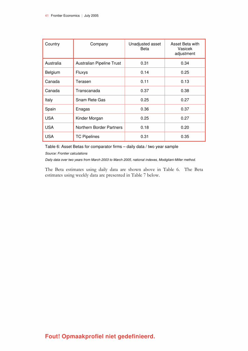
41 Frontier Economics | July 2005
Fout! Opmaakprofiel niet gedefinieerd.
Country Company Unadjusted asset Beta
Asset Beta with Vasicek
adjustment
Australia Australian Pipeline Trust 0.31 0.34
Belgium Fluxys 0.14 0.25
Canada Terasen 0.11 0.13
Canada Transcanada 0.37 0.38
Italy Snam Rete Gas 0.25 0.27
Spain Enagas 0.36 0.37
USA Kinder Morgan 0.25 0.27
USA Northern Border Partners 0.18 0.20
USA TC Pipelines 0.31 0.35
Table 6: Asset Betas for comparator firms – daily data / two year sample
Source: Frontier calculations
Daily data over two years from March 2003 to March 2005, national indexes, Modigliani-Miller method.
The Beta estimates using daily data are shown above in Table 6. The Beta estimates using weekly data are presented in Table 7 below.

42 Frontier Economics | July 2005
Fout! Opmaakprofiel niet gedefinieerd.
Country Company Unadjusted asset Beta
Asset Beta with Vasicek
adjustment
Australia Australian Pipeline Trust 0.15 0.21
Belgium Fluxys 0.14 0.28
Canada Terasen 0.09 0.11
Canada Transcanada 0.03 0.06
Italy Snam Rete Gas 0.16 0.19
Spain Enagas 0.22 0.27
USA Kinder Morgan 0.36 0.40
USA Northern Border Partners 0.16 0.19
USA TC Pipelines 0.14 0.20
Table 7: Asset Betas for comparator firms – weekly data / five year sample
Source: Frontier calculations
Weekly data over five years from March 2000 to March 2005, national indexes, Modigliani-Miller method.
The choice of the appropriate range for the Beta estimate used for GTS is based on an assessment of the average, the 25th percentile and the 75th percentile over the sample of comparator firms (as described in more detail above). The analysis is based on the comparator asset Beta values after the Vasicek adjustment has been applied30. These results are shown in Table 8.
The average Beta from the daily and the weekly estimates establishes an appropriate range of the Beta for GTS.
Asset Beta Daily 2 year Week 5 year
25th percentile 0.25 0.19
Mean 0.29 0.21
75th percentile 0.35 0.27
Table 8: Asset Beta range for GTS
Source: Frontier calculations
30 For example, if the unadjusted comparator asset betas were used the range for GTS’s asset beta would 0.18 to 0.31 based on the daily estimates, and 0.14 to 0.16 based on the weekly estimates.
43 Frontier Economics | July 2005
Fout! Opmaakprofiel niet gedefinieerd.
Summary on the Beta
The asset Beta has been estimated based on a sample of quoted companies whose primary activity is gas transportation. The final Beta estimates have been obtained using two approaches: daily data over the last two years and weekly data over the past five years.
For the WACC calculation for GTS we would propose a range for the asset Beta of 0.21 to 0.29 – based on the average of the daily and the average of the weekly estimates.
4.5 GEARING, TAX AND INFLATION
The previous sections have described the issues involved in estimating the cost of equity and the cost of debt. The remainder of this section outlines the issues raised by the remaining parameters: gearing, tax and inflation.
4.5.1 Gearing
Gearing is the measure of the proportion of the finance in the business that is provided by debt investors. For a company with published accounts a measure of gearing can be easily obtained from the accounting data (net debt as a % of shareholders’ funds plus net debt). However, the appropriate measure of gearing for estimating the WACC is the market value of debt as a % of the market value of the company.
Utility regulators typically calculate the WACC based on a ‘notional’ level of gearing rather than the actual gearing levels for the companies31. This approach has a number of advantages:
• the regulator can identify a range of gearing that is consistent with efficient financing cost – a gearing range that balances the tax advantages of debt with the cost of default risk;
• simplicity – it is not necessary for the regulator to collect and analyse detailed information on each company’s capital structure; and
• this approach ensures a consistent treatment across companies when the regulator is setting the WACC for a number of companies within the same industry.
We propose that the WACC for GTS is calculated based on a gearing level of 60%. It should be emphasised that this is an assumed gearing level and DTe is not suggesting that GTS’s actual gearing level need necessarily coincide with this assumption. Indeed it is a matter for the company to determine its own efficient gearing level.
The 60% assumption is considered reasonable for a number of reasons.
31 See CEPA report, An international comparison of the regulated cost of capital, February 2005.

44 Frontier Economics | July 2005
Fout! Opmaakprofiel niet gedefinieerd.
… Consistency with other regulatory decisions - The CEPA study undertaken for DTe shows that a gearing assumption of 60% is consistent with the decisions of other utility regulators.
… Consistency with actual gearing levels in comparator companies - Table 3 provides details of the gearing level of the comparator companies used to estimate the debt premium. This suggests that gearing for similar companies with investment grade credit ratings can vary (from around 40% to around 70%) but a gearing of 60% is consistent with the financing choices of these companies.
… Consistency with investment grade credit rating - Given the relatively low risk regulatory regime (for example, the cost-plus nature of the regime) and the expected low level of business risk that GTS faces, a gearing level of 60% should enable GTS to maintain a solid investment grade rating. As a result the gearing assumption is consistent with the identified value for the debt premium.
4.5.2 Taxation
In setting price controls a regulator has a number of options for the treatment of taxation in the cost of capital. A regulator has two separate choices to make:
• first, whether to include the impact of corporation tax within the estimate of the rate of return or whether to treat it as a separate cost item;
• second, whether the allowance for corporation tax should be based on the standard corporation tax rates or a projection of the amount of tax that the company will actually pay (known as the effective tax rate).
The first choice has clear implications for the appropriate definition of the WACC to be used to set the rate of return:
• if tax is included in the rate of return then a pre-tax WACC should be used to set the rate of return; and
• if tax is excluded from the rate of return, and treated as a separate item in the revenue calculation, then a post-tax WACC should be used to set the rate of the return.
DTe is not expected to treat tax as a separate cost item when assessing the revenue cap for GTS for the period 2006 to 2009. A pre-tax WACC is therefore appropriate. The CEPA report for DTe also shows that the majority of regulators adopt an approach of setting a pre-tax rate of return based on standard corporation tax rates. This is the approach adopted for setting a WACC for GTS.
The standard corporation tax rate in the Netherlands is currently 35% but it has been announced that the rate will be reduced to 30% by the end of the price control period. In calculating the WACC we have assumed a value of 30%.

45 Frontier Economics | July 2005
Fout! Opmaakprofiel niet gedefinieerd.
4.5.3 Inflation and the real WACC
The earlier discussion on the risk-free rate related to the nominal risk-free rate. This evidence will feed into the calculation of a nominal WACC for GTS. To convert this to a calculation of the real WACC to be used in setting the price control it is necessary to adjust the nominal WACC by an appropriate projection of the inflation rate32. This raises a number of practical issues.
… Adjusting nominal rates for inflation forecasts. The inflation rate applied to the nominal WACC should be consistent with the inflation expectations that underpin the data on the nominal risk-free rate. This could be based on current inflation rates and / or published inflation forecasts.
… Use of index-linked debt yields. The real risk-free rate that is implied by the inflation rate assumption can be benchmarked to data on the yields on index-linked debt. For example, the French government has issued index-linked bonds that are based on Euro-zone inflation and this could be a relevant source of data to estimate the real risk-free rate for the Netherlands.
Table 9 shows the implied real risk-free rate based on the range for the nominal risk-free rate identified above. The inflation rate of 1.5% used in the Table corresponds to the medium term forecast by the CPB.
Low High
Nominal risk-free rate 4.0% 4.5%
Inflation rate 1.5% 1.5%
Real risk-free rate 2.5% 3.0%
Table 9: Implied real risk-free rate
Source: Netherlands Central Bank, Frontier calculations
32 The formula for converting from nominal to real is: real = [(1+nominal)/(1+inflation)-1]. When inflation and interest rates are low this is closely approximated by: real = nominal – inflation.

46 Frontier Economics | July 2005
Fout! Opmaakprofiel niet gedefinieerd.
5 WACC calculation for GTS
Table 10 shows the calculation of the pre-tax WACC for GTS based on the parameters identified in the previous section. The range for the real pre-tax WACC is 4.6% to 6.2%.
Low High
Nominal risk-free rate 4.0% 4.5%
Debt premium 0.8% 0.8%
Cost of debt 4.8% 5.3%
Equity risk premium 4.0% 6.0%
Asset beta 0.21 0.29
Equity beta 0.43 0.59
Cost of equity 5.7% 8.0%
Gearing 60% 60%
Tax rate 30% 30%
Nominal pre-tax WACC 6.1% 7.8%
Inflation 1.5% 1.5%
Real pre-tax WACC 4.6% 6.2%
Table 10: Estimate of the real pre-tax WACC for GTS
Source: Frontier Economics calculations
The estimated range of 4.6% to 6.2% is appropriate for a number of reasons.
… The methodology is robust and consistent with regulatory best practice - as discussed in Section 3 the CAPM is considered to be the most robust available methodology for calculating the WACC. Furthermore, the methodology is used by the majority of regulators and by companies. It is therefore consistent with best practice for estimating the WACC.
… The estimates of the parameter values have been rigorously determined and are considered reasonable – as discussed in Section 4, care has been taken to ensure that the estimates for each of the parameter values in the WACC formula are consistent with available financial evidence and are

47 Frontier Economics | July 2005
Fout! Opmaakprofiel niet gedefinieerd.
consistent with both financial theory and regulatory precedence. In particular:
• the value of the nominal risk-free rate is consistent with the average yield on 10-year government debt in the Netherlands over a horizon of upto five years;
• the value of the debt premium is based on a rigorous assessment of comparator data for similar companies with an investment grade credit rating;
• the estimate of the equity risk premium is consistent with international evidence on the ERP, survey evidence and evidence from models of ERP expectations;
• the asset beta value is based on an in-depth analysis of comparator data for similar companies – with a range of methodologies for estimating betas assessed – and incorporates a Bayesian adjustment and conversion from equity betas using the standard Modigliani-Miller formula;
• the equity beta is directly converted from the asset beta estimate using the assumed gearing level and the level is consistent with the low risk regulatory regime that DTe expects to apply to GTS;
• the gearing level is consistent with the levels assumed by other regulators and with the gearing levels of similar companies;
• the tax rate is equal to the corporation tax rate that GTS is currently expected to face during the regulatory period; and
• the inflation rate is consistent with the medium term inflation forecast of the CPB.


49 Frontier Economics | July 2005
Fout! Opmaakprofiel niet gedefinieerd.
Annexe 1: Selection of comparators for Beta calculation
INTRODUCTION
This annexe describes the procedure that Frontier followed to create a shortlist of international comparators for GTS. The list of comparators includes 9 companies from 6 countries.
PROCEDURE TO IDENTIFY COMPARATORS
Frontier identified the list of comparators following a two-stage process:
• first, we created an inclusive list of quoted companies with gas transportation operations, and
• second, we chose companies that appeared to be most suitable based on the summary information available on them.
The following sections describe the sources we used to identify the quoted companies, and the criteria we applied to choose the set of comparators.
IDENTIFYING THE QUOTED COMPANIES
To create a list of quoted companies with gas transportation operations in the developed countries, Frontier relied on the following sources:
• input from Frontier country energy experts;
• Frontier report for DTe “Regulation of European gas transmission system operators” (December 2004);
• other comparative studies, such as the NECG report “International comparison of WACC decisions” (September 2003); and
• proprietary financial databases to which Frontier is a subscriber (Thomson Financial), supplemented by information from company websites and latest annual reports.
CHOOSING COMPARATORS
Frontier applied the following general principles to choose the set of comparators among the quoted companies.
… Network operations should be significant: gas transportation should comprise a substantial, ideally dominant, part of companies’ activities.
… All company operations should be similar in terms of their risk characteristics. This includes the following aspects:

50 Frontier Economics | July 2005
Fout! Opmaakprofiel niet gedefinieerd.
• diversification to other industries with markedly different risk profiles (e.g., financial investment industry, residential construction) should be minimised;
• to the extent that a company is involved in non-energy operations, those should preferably fall within the utilities sector;
• within the energy sector, diversification to other products (oil, propane etc) and other stages of the supply chain (upstream production, downstream energy services) should be minimised where possible.
… Quoted companies should be large enough to ensure that there is active trading and sufficient price variation for their stock.
… Regulatory regime should be comparable to the one in Netherlands. In particular, we excluded countries for which information about the nature of their regulatory regime is not available.
LIST OF COMPARATORS FOR GTS
The list of comparator companies for GTS, and the relevant characteristics of these companies33, is shown in the Figure below.
33 Company size is indicated by the value of turnover and the value of assets. Exposure to capital cost risk is indicated by the ratio of capital expenditure (CAPEX) to turnover.

51 Frontier Economics | July 2005
Fout! Opmaakprofiel niet gedefinieerd.
Country Company Gas transport share1 Other activities Regulation Turnover, mln EUR
Assets, mln EUR
Australia Australian Pipeline Trust 95% Trade & supply Price cap, 5 yrs
145 845
Belgium Fluxys 100% Cost of service, 1 yr 385 1.836
Canada Terasen 50% Distribution, trade Rate of return 1.221 3.102
Canada TransCanada 75% Production Rate of return 3.187 13.809
Italy Snam Rete Gas 95% Trade & supply Ex-ante cost-plus, 1 yr
1.758 9.813
Spain Enagas 100% Ex-ante cost-plus, 1 yr
1.570 3.093
USA Kinder Morgan Energy 100% Rate of return
4.978 6.868
USA Northern Border Partners 80% Production Rate of return
418 1.932
USA TC Pipelines 100% Rate of return n/a n/a
Table 11: Comparator characteristics
Source: Frontier calculations based on annual reports, financial statements, company websites.
1May include storage, LNG terminals and pipelines of other products. Share based on income data, or on asset data if income data not available (in all cases where both measures
were available, the difference did not exceed 5%). Numbers rounded to 5% increments to reflect data limitations.


Frontier Economics Limited in Europe is a member of the Frontier Economics network, which consists of separate companies based in Europe (London & Cologne) and Australia (Melbourne & Sydney). The companies are independently owned, and legal commitments entered into by any one company do not impose any obligations on other companies in the network. All views expressed in this document are the views of Frontier Economics Limited.


THE FRONTIER ECONOMICS NETWORK
LONDON | COLOGNE | MELBOURNE | SYDNEY
Frontier Economics Ltd 71 High Holborn London WC1V 6DA
Tel. +44 (0)20 7031 7000 Fax. +44 (0)20 7031 7001 www.frontier-economics.com


