Running Head: DE Gap in Risky and Ambiguous Gambles 1

In Press: Journal of Behavioral Decision Making

The Description-Experience Gap in Risky and Ambiguous Gambles

Varun Dutt1, 4, Horacio Arló-Costa2, Jeffrey Helzner3, and Cleotilde Gonzalez4

1 School of Computing and Electrical Engineering, School of Humanities and Social Sciences,

Indian Institute of Technology, Mandi, India

2 Department of Philosophy, Carnegie Mellon University, USA

3 Department of Philosophy, Columbia University, USA

4 Dynamic Decision Making Laboratory, Department of Social and Decision Sciences, Carnegie

Mellon University, USA

Word Count: 9,548 words

Author Note

This research was supported by a Defense Threat Reduction Agency (grant number:

HDTRA1-09-1-0053) and by the National Science Foundation (grant number: 1154012) awards

to Cleotilde Gonzalez. The authors are thankful to Hau-yu Wong, Dynamic Decision Making

Laboratory, Carnegie Mellon University for providing comments on the manuscript. This

manuscript is dedicated to the memory of Professor Horacio Arló-Costa, our collaborator and

friend to whom we owe many of the reported ideas. Correspondence concerning this article

should be addressed to Prof. Varun Dutt, School of Computing and Electrical Engineering,

School of Humanities and Social Sciences, Indian Institute of Technology, Mandi, PWD Rest

House 2nd Floor, Mandi - 175 001, H.P., India. Email: varun@iitmandi.ac.in

Running Head: DE Gap in Risky and Ambiguous Gambles 2

Abstract

Recent research in decision making reported a description-experience (DE) gap: opposite risky

choices when decisions are made from descriptions (gambles in which probability distributions

and outcomes are explicitly stated) and when decisions are made from experience (the

knowledge of the gambles is obtained by sampling outcomes from unknown probability

distributions before making a choice). The DE gap has been reported in gambles commonly

involving a risky option (outcomes drawn from a fixed probability distribution) and a safe option

(probability of the outcome is 1); or, in gambles involving two risky options. Here, we extend the

study of the DE gap to gambles in which people choose between a risky option and an

ambiguous option (with two nested probability distributions, where the event-generation

mechanism is more opaque than that in the risky option). We report empirical evidence and show

a DE gap in gambles involving risky and ambiguous options. Participants choices are influenced

by the information format and by the ambiguous option: participants are ambiguity-seeking in

experience and ambiguity-averse in description in problems involving both gains and losses. In

order to find reasons for our results, we investigate participants’ sampling behavior and this

analysis indicates choices according to a cognitive model of experiential decisions (Instance-

Based Learning). In experience, participants have small sample-sizes and participants choose

options where high outcomes are experienced more frequently than expected. We discuss the

implications of our results for the psychology of decision making in complex environments.

Keywords: risk, ambiguity, Instance-Based Learning Theory, decisions from experience,

ambiguity aversion, complex environments.

Running Head: DE Gap in Risky and Ambiguous Gambles 3

The Description-Experience Gap in Conditions Involving Risk and Ambiguity

Benjamin Franklin famously stated that the only things certain in life are death and taxes.

In many decisions we make, we face different options with varying degrees of ambiguity. While

we might be able to attach specific probabilities to different outcomes in certain problems (e.g.,

the probability of getting a “3” when throwing a fair die; Hertwig, in press), we may encounter

certain events where assessing a precise probability value is not possible (e.g., when predicting

the precise probability of a future global-warming catastrophe; Dutt & Gonzalez, 2012). The

economist Frank Knight (1921) made an initial conceptual distinction between decisions under

risk (“measurable probabilities”) and decisions under ambiguity (“unmeasurable probabilities”)

(pg. 20). Therefore, risk refers to decisions where the decision maker knows with certainty the

mathematical probabilities of possible outcomes for choice options; in contrast, ambiguity refers

to decisions where the likelihoods (probabilities) of different outcomes are vague and cannot be

expressed with any mathematical precision (Knight, 1921; Luce & Raiffa, 1957; Rakow &

Newell, 2010).

For risky decisions, an increasing body of research indicates that choices between options

depend on how information about probabilities and outcomes is learned. Researchers have made

use of a “sampling paradigm” in decisions made from “experience” where people first sample as

many outcomes as they wish from an option with defined probability distributions (that are

unknown to participants), and then decide from which option to make a single draw for real

(Hertwig, Barron, Weber & Erev, 2004; Hertwig & Erev, 2009). In contrast, when decisions are

made from “description,” the information about the possible outcomes from an option and their

probability distribution are given to the participants and they make a selection between different

options (Hertwig et al., 2004). In both experience and description, people are asked to either

Running Head: DE Gap in Risky and Ambiguous Gambles 4

choose between two risky options (each with a single probability distribution), or to choose

between a risky option and a safe option (where probability = 1). For descriptive decisions,

people behave as if rare (low probability) outcomes receive more impact than they deserve

according to their objective probability; whereas, for experiential decisions, people behave as if

rare outcomes receive less impact than they deserve (Gonzalez & Dutt, 2011; Hertwig, Barron,

Weber, & Erev, 2004; Hertwig & Erev, 2009; Weber, Shafir, & Blais, 2004). This phenomenon

has been called the description-experience (DE) gap in decisions under risk, and it seems to hold

for problems involving both gains and losses.1

Like risk, decisions under ambiguity could also be presented to participants in either a

descriptive or an experiential form. However, the probabilities of outcomes in the ambiguous

option cannot be expressed with any mathematical precision (Rakow & Newell, 2010), and the

question is how to distinguish ambiguity from risk? One possibility proposed by Arló-Costa and

colleagues (Arló-Costa and Helzner, 2009; Arló-Costa, Dutt, Gonzalez, and Helzner, 2011) is to

distinguish ambiguity from risk in terms of the number of random variables that determine the

outcomes, i.e., the number of probability distributions needed to determine the outcome of a

choice.

2

1 In decisions under risk, the DE gap is defined as participants’ risky choices in experience minus their

risky choices in description (Hertwig et al., 2004).

Typically, in decisions under risk, the outcome of a choice is determined by a single

random variable (one probability distribution) (Hertwig & Erev, 2009). However, one way of

making the same risky option ambiguous might be to break this single random variable (one

2 A random variable conceptually does not have a single, fixed value (even if unknown); rather, it can take

on a set of possible different values, each with an associated probability. In this paper, the risky option has a single

random variable; however, the ambiguous option has two random variables.

Running Head: DE Gap in Risky and Ambiguous Gambles 5

probability distribution) into equivalent two nested random variables (two probability

distributions), such that the working of both these events now determines the resulting outcome.

We refer to conditions in which the outcome of a choice is determined by two or more

probability distributions as ambiguous, to distinguish it from risky conditions (one probability

distribution) but also to acknowledge that this event-generation mechanism is not really an

ambiguous one in the Ellsberg sense (see discussion below), but instead simply more opaque

than the one probability distribution risky mechanism.

The idea of two or more nested probability distributions in decisions under ambiguity is

common in many natural decision making situations (Gonzalez, Vanyukov & Martin, 2005;

Gonzalez, Lerch & Lebiere, 2003). For example, when we want to collect information about a

product, we first select a source (e.g., a store; the first random variable), and then get samples

from this source (answers to questions; the second random variable). Similarly, when deciding

between several garments (each placed in a separate rack in a store), we might first select a rack

(first random variable) and then decide to get samples from the chosen rack (the second random

variable). Up to now, research has paid little attention to the description – experience gap (DE

gap) in gambles where the options differ in the number of random variables.

In this paper, we set two explicit goals. First, we determine the degree of people’s

aversion to ambiguity when people are presented simultaneously with the same option as either

risky (one random variable) or ambiguous (more than one random variables) in a descriptive

form. Second, we contrast this descriptive situation with a similar situation now presented in the

sampling paradigm to determine people’s attitude to ambiguity in decisions from experience.

Thus, we test whether the additional complexity in the ambiguous option results in ambiguity-

aversion in decisions from description; and, more importantly, whether this additional

Running Head: DE Gap in Risky and Ambiguous Gambles 6

complexity can lead to ambiguity-seeking in decisions from experience. In other words, is there a

DE gap when people are asked to choose between a risky option and an ambiguous option,

where the options differ on the number of random variables?

Decisions under Risky and Ambiguous Conditions

In contrast to a risky option, in an ambiguous option all possible values of probability

(between 0 and 1) could be assumed to be equally likely, with the midpoint of the range of

possible likelihoods (e.g., .5) as the best estimate (Weber & Johnson, 2008). However, Ellsberg

(1961) showed that when presented with described risky and ambiguous options, people have a

clear preference for the former rather than the latter – a behavior that Ellsberg called ambiguity

aversion. Ambiguity aversion has been observed in both laboratory experiments and in real-

world health, environmental, and negotiation contexts (Camerer & Weber, 1992; Curley &

Yates, 1989; Hogarth & Kunreuther, 1989; Wakker, 2010). For example, Camerer and Weber

(1992) provided a thorough review of the literature on decisions under ambiguity and showed

that ambiguity aversion is a very stable phenomenon observed in a large number of described

problems.

Although ambiguity aversion prevails robustly for described gains, the case is less clear

for described losses (Wakker, 2010). For losses, some researchers found ambiguity aversion

behavior (Keren & Gerritsen, 1999), some found mixed evidence (Cohen, Jaffray, & Said, 1987;

Dobbs, 1991; Hogarth & Kunreuther, 1989; Mangelsdorff & Weber, 1994; Viscusi & Chesson,

1999), and a number of researchers found ambiguity seeking behavior (Abdellaoui, Vossman, &

Webber, 2005; Chakravarty & Roy, 2009; Davidovich & Yassour, 2009; Di Mauro &

Maffioletti, 2002; Du & Budescu, 2005; Einhorn & Hogarth, 1986; Ho, Keller, & Keltyka,

2002).

Running Head: DE Gap in Risky and Ambiguous Gambles 7

Ambiguity aversion is a well-known phenomenon in decisions from description.

However, very little is currently known about ambiguity aversion in situations involving

experiential decisions. In fact, although the study of the DE gap has been prominent for risky

decisions, the existence of a similar gap for a choice between risky and ambiguous decisions, has

yet to be investigated. Such research that shows a DE gap becomes important because some

researchers have described experiential decisions under risk to be similar to decisions involving

ambiguity (Fox & Hadar, 2006; Hadar & Fox, 2009). According to Hadar and Fox (2009),

decisions from experience apply to any situation in which there is ambiguity and learning

through trial-and-error feedback (i.e., sampling of outcomes). However, Hadar and Fox (2009)

do not say anything about what it means to have an experiential counterpart to a given

description in decisions under ambiguity, an assumption that is crucial to the equivalence of

descriptive and experiential decisions and to the study of the D-E gap in decisions under

ambiguity.

Arló-Costa and Helzner (2009) and Arló-Costa, Dutt, Gonzalez, and Helzner (2011) have

defined decisions from description and experience so that one could create equivalent

experiential and descriptive counterparts for problems involving ambiguity. According to Arló-

Costa et al. (2011), in risky options people are presented with a specification of a chance

mechanism; whereas in ambiguous options people are not presented with such a specification,

rather they are allowed to observe the behavior of the chance mechanism. In this sense, while

classical descriptions under ambiguity (e.g., the Ellsberg’s problem) have no experiential

counterparts since the relevant ambiguities in such cases are epistemic, one can specify random

variables (probability distributions) that, at least psychologically, approximate the descriptions of

ambiguities and have an experiential counterpart. Having this experiential counterpart to the

Running Head: DE Gap in Risky and Ambiguous Gambles 8

description in decisions under ambiguity enables us to extend the study of the DE gap in

decisions under risk to decisions under ambiguity. Thus, a possibility is to make participants

perceive an option as risky or ambiguous by the number of random variables that generate the

outcomes: one random variable in decisions under risk and two or more nested random variables

in decisions under ambiguity. The difference created between risky and ambiguous options based

upon the number of random variables could be a sufficient condition to test the DE gap in

decisions under ambiguity. However, one does need to note that our differentiation between

risky and ambiguous options that is based upon number of random variables is different from the

distinction made in the classic Ellsberg sense between risky and ambiguous options.

Given this difference, a goal of this paper is to determine choice when people are

presented simultaneously with described risky and ambiguous options that differ in terms of the

number of random variables. Second, we develop an experiential paradigm to extend the study of

the DE gap in risky decisions to ambiguous decisions. The main questions we ask are the

following: Is there a DE gap in ambiguous conditions? If so, what could be the reasons for this

gap? We answer the first question by reporting an experiment where human participants make

choices between risky and ambiguous options in descriptive and (approximate) experiential

counterparts of the Ellsberg’s problem. In order to probe the reasons for our experimental

findings, we first analyze participants’ trial-and-error learning (sampling) in experience. This

analysis qualitatively compares experiential decisions in the ambiguous conditions to

experiential decisions under risk. In past research, risky choices from experience has been

explained based upon the cognitive processes proposed by the Instance-based Learning Theory

(IBLT), a theory of decisions from experience in dynamic tasks (Gonzalez, Lerch, & Lebiere,

2003) and a simple computational model derived from the theory for binary-choice tasks

Running Head: DE Gap in Risky and Ambiguous Gambles 9

(Gonzalez & Dutt, 2011). The IBL model presents a process in which decisions are made from

stored and retrieved experiences (called instances), based upon small samples and recently and

frequently experienced outcomes. We expect that these cognitive processes would apply to both

risky and ambiguous conditions from experience. Thus, we generate our hypotheses from the

cognitive processes implemented in the IBL model as well as the literature in decisions from

experience. We close this paper by drawing insights from this research effort to the psychology

of complex decisions and decisions under ambiguity and on how these situations compare with

decisions under risk.

Representing Experience in Decisions under Ambiguity

Consider the classical Ellsberg’s two-color problem (Ellsberg, 1961):

Urn A contains exactly 100 balls. 50 of these balls are solid black and the remaining 50

are solid white.

Urn B contains exactly 100 balls. Each of these balls is either solid black or solid white,

although the ratio of black balls to white balls is unknown.

Consider now the following questions: How much would you be willing to pay for a ticket

that pays $25 ($0) if the next random selection from Urn A results in black (white) ball? Repeat

then the same question for Urn B.

Urn B is ambiguous as the ratio of black to white balls in unknown, while urn A is not. It

is a well-known result that a majority of participants prefer urn A to urn B and also decide to

make greater payments for urn A than urn B (Ellsberg, 1961; Tversky & Fox, 1995). Tversky

and Fox (1995) explained participants’ ambiguity aversion in the Ellsberg’s problems with the

comparative ignorance hypothesis. Their hypothesis was that people are only ambiguity-averse

when their attention is specifically brought to the ambiguity by comparing an ambiguous option

Running Head: DE Gap in Risky and Ambiguous Gambles 10

(urn B) to an unambiguous option (urn A). For instance, people are willing to pay more on

choosing a correct colored ball from an urn containing equal proportions of black and white balls

than an urn with unknown proportions of balls when evaluating both of these urns at the same

time. When evaluating them separately, however, people are willing to pay approximately the

same amount on either urn. However, Arló-Costa and Helzner (2005, 2007) have recently shown

that people seem to behave as ambiguity-averse even in non-comparative cases when urn A and

B are not presented simultaneously. One reason for ambiguity aversion in the non-comparative

cases could be that people form implicit assumptions to deal with the ambiguity resulting from

the unknown information about urn B; and these assumptions might lead them to behave as

ambiguity-averse (Guney & Newell, 2011).

In Ellsberg’s problem, it is next to impossible to have an experiential counterpart for urn

B because the probabilistic information is ambiguous. That is because the ratio of black to white

balls is unknown and so one cannot simulate the process as an experience. Rakow and Newell

(2010) have provided a continuum of types of ambiguity/probability, the degrees of uncertainty.

According to these researchers, anchored at one end are risky decisions of perfect regularity

where probabilities can be determined precisely, with the other extreme being ambiguous

decision situations where only an estimate of the probability could be used to determine one’s

belief. From the decision maker’s perspective, these decision extremes differ according to how

easily the outcomes’ probability distributions can be calculated. Considering these degrees of

uncertainty, urn A is of the former risky decision type (with a precise definition of the

probability), while urn B is of the latter ambiguous decision type (with an imprecise definition of

the probability). According to Rakow and Newell (2010), risky decisions from experience

generally tend to occupy a middle ground between the extremes in the degrees of uncertainty.

Running Head: DE Gap in Risky and Ambiguous Gambles 11

Thus, the probability of the outcomes is not precisely known in risky decisions from experience,

but it could be empirically determined by observation (sampling) of outcomes. If we want to

evaluate the DE gap in Ellsberg’s problem, then we need to develop an experiential middle

ground between urns A and B for the ambiguous information in urn B to be performed

experientially. One way of doing so is to convert the single random variable (i.e., a probability

distribution) that determines the probability in the risky option into two random variables (i.e.,

two probability distributions) that are likely to be perceived as the ambiguous option. Although

this setup is different from the classical Ellsberg’s problem, Arló-Costa and Helzner (2005,

2007) have used this idea to propose the following descriptive chance setup:

B*: First, select an integer between 0 and 100 at random, and let n be the result of this

selection. Second, make a random selection from an urn consisting of exactly 100 balls, where n

of these balls are solid black and 100 - n are solid white.

In B*, the first selection between 0 and 100 (i.e., the first random variable) is like picking

an urn with a certain distribution of black and white balls. Once the first selection is made, the

second selection (i.e., the second random variable) is the act of playing the urn that was picked in

the first selection. In a number of experiments, Arló-Costa and Helzner (2005, 2007) and Arló-

Costa et al. (2011) have shown that participants’ payments for B* are in between those for urns

A and B. For example, Arló-Costa et al. (2011) report that payments for urn A (=$7.04) were

greater than those for B* (=$6.36), and those for B* were greater than those for urn B (=$4.93).

Thus, people prefer an option (A), which depends on one risky random variable, over an option

(B*), which depends on two risky random variables. Also, people prefer an option (B*), which

depends on two risky random variables, over an option (B), where the specification of random

variables is ambiguous. Chow and Sarin (2002) and Yates and Zukowski (1976) reported similar

Running Head: DE Gap in Risky and Ambiguous Gambles 12

results using B*. These results show that people consider B* to be of intermediate ambiguity

between the ambiguous urn B and the unambiguous urn A, and that one reason for these findings

could be the inability to reduce the compound lottery B* (containing two random variables) to

the simple lottery A (Halevy, 2007). This line of reasoning might be plausible because B* is

mathematically equivalent to A.3

More importantly, the perception of B* as being more ambiguous than A is very useful as

it allows us to treat B* as an operational approximation of urn B in experience. Again, the

interest of this move is that B* is easily implementable in experience, while it is notoriously

difficult to find an experiential counterpart of urn B. The way we do in this paper is by making

option B more ambiguous in option B* by introducing two random variables that determine the

outcomes.

Also, The pattern of preference between A, B*, and B suggests

that part to the indication for ambiguity-aversion can be related to a tendency to prefer simpler

options, which have fewer or well-defined random variables.

Experiment: The DE Gap in Decisions under Risk and Ambiguity

In this section, we report an experiment that tests for the DE gap by utilizing the

formulations of urn A and B* in description and experience.

Hypotheses

Our goal was to compare the difference in people’s ambiguity- seeking/aversive

predisposition for outcomes presented as a written description or as an experience (i.e., the DE

3 The line of reasoning is roughly as follows: The random selection in the first stage of B* entails that, for each integer i, where 0 ≤ i ≤ 100, there is a probability of that the urn sampled in the second stage consists of i black balls and 100 - i white balls. Moreover, according to this line of reasoning the random selection in the second stage entails that if i is selected in the first stage, then the probability of selecting a black ball in the second stage is

. This line of reasoning then continues by combining the first and second stage probabilities to conclude that the

probability of getting a black ball on any trial of B* = , exactly as in the case of urn A.

Running Head: DE Gap in Risky and Ambiguous Gambles 13

gap for ambiguity) in problems involving risky and ambiguous options. Given the overwhelming

evidence of the existence of the DE gap in decisions under risk (e.g., Hertwig et al., 2004;

Hertwig & Erev, 2009) where decision makers make decisions based upon recency and

frequency of experienced outcomes (explained by IBLT) and the arguments above that risk and

ambiguity are a part of a continuum of degrees of uncertainty (Rakow & Newell, 2010), we

expect a similar DE gap in decisions under ambiguity. More specifically, as people are shown to

be ambiguity-averse in description in a large number of studies in decisions under ambiguity

(Camerer & Weber, 1992; Curley & Yates, 1989; Hogarth & Kunreuther, 1989; Wakker, 2010),

we expect them to be less ambiguity-averse in experience. This expectation is based upon the

assumption that decision makers can distinguish between one or more than one random variables

that determine the outcomes in risky and ambiguous options in experience, respectively. Here,

according to the IBL model's predictions (Gonzalez & Dutt, 2011), participants are likely to

choose an option (risky or ambiguous) where participants encounter a high (maximizing)

outcome more recently and frequently (based upon the IBLT assumptions of recency and

frequency). Thus, if participants more frequently and recently encounter higher payoffs during

their sampling in the ambiguous option, then they are likely to choose the ambiguous option

during their final choice in experience. Therefore, we expect:

H1: A greater proportion of participants will be ambiguity-seeking in experience

compared with description.

Furthermore, the DE gap in decisions under risk has been reported for both gains and

losses (Hertwig et al., 2004; Hertwig & Erev, 2009). Whether one considers gains or losses, the

nature of the gap is driven by underweighting rare outcomes in experience and overweighting

rare outcomes in description. Moreover, in decisions under ambiguity, people have been found to

Running Head: DE Gap in Risky and Ambiguous Gambles 14

be ambiguity-averse for gains and there currently exists mixed evidence for losses (Wakker,

2010). Thus, in decisions under ambiguity, we expected people to be ambiguity-averse in

description and less ambiguity-averse in experience for both gains and losses. Therefore, we

expect:

H2: A greater proportion of participants will be ambiguity-seeking in experience

compared with description irrespective of gains and losses.

Method

Participants. One hundred and fifty-three participants were randomly assigned to one of

two conditions, description (N=61) and experience (N=92).4

4 Both the description and experience conditions contained a large number of participants (> 50). The data

in the two conditions was collected at the same time, where participants could only participate once in the study. The

difference in number of participants between the two conditions was due to participants signing-up but not turning-

up for the study on a particular day. The difference in the number of participants between the two conditions does

not create a problem because in our results we found that the distributions different preference strengths were similar

across the two conditions.

Seventy-six participants were male

and the rest were female. The mean age was 26 years (S.D. = 8), and ages ranged from 18 to 63

years. All participants received a base payment of $5 for participating in the experiment which

lasted for less than 20 minutes. In addition, participants could earn performance bonuses based

upon the outcomes they received in the gain and loss problems. Participants could win $25 or $0

in the gain problem and they could lose $25 or $0 in the loss problem. The final earnings across

the two problems were added up into a total, and the total was scaled in the ratio 10:1 to pay

participants their performance bonuses. For example, total earnings of $25 across the two

problems (i.e., $25 in the gain problem and $0 in the loss problem) would give a participant

Running Head: DE Gap in Risky and Ambiguous Gambles 15

$2.50 as performance bonus in addition to their $5 base pay. Thus, in the worst case, a

participant would get $2.50 from the study (i.e., $5 base payment + $0 in the gain problem -

$2.50 in the loss problem).

Experimental design. We operationalized the definition of urn A and B* by employing

the following descriptions for gain and loss problems in terms of fair chance setups (or random

variables).

A: A fair chance setup with possible outcomes {1, 2, … , 99, 100} has been constructed. If

the outcome on the next run of this setup is less than or equal to 50, then you win (lose) $25.

Otherwise, you get $0. (risky option)

B*: Two fair chance setups, I and II, have been constructed. Setup I has possible

outcomes {0, 2, … , 99, 100}. Setup II has possible outcomes {1, 2, … , 99, 100}. The game is

played by first running setup I and then running setup II. If the outcome of the run of setup II is

less than or equal to the outcome from the run of setup I, then you win (lose) $25. Otherwise, you

get $0. (ambiguous option)

A is the risky option and B* is the ambiguous option based upon the specification of one

or two random variables, respectively (hereafter, A will be referred to as risky and B* as

ambiguous option). Both risky and ambiguous options are either framed as a win in one problem

(gain problem), or as a loss in the other problem (loss problem). We use the above two

descriptions of the risky and ambiguous options as part of the description condition in the

experiment. In the experience condition, the text for the risky and ambiguous options is replaced

by button options that can be sampled repeatedly before making a final choice as is done in the

traditional sampling paradigm (see Hertwig and Erev (2009) for example). The proportion of

ambiguous (B*) choices indicated the degree of ambiguity-seeking across description and

Running Head: DE Gap in Risky and Ambiguous Gambles 16

experience, and this proportion served as the main dependent variable for the purposes of

statistical analysis.

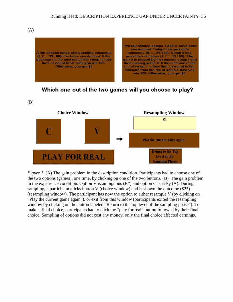
Description condition. Each participant assigned to this condition was presented with

two problems in a random order. One of the problems was a gain problem (win $25 or $0), while

the other was a loss problem (lose $25 or $0). In each problem, participants faced a computer

window with two large buttons (representing the two games or options) that were labeled with

text descriptions for the risky (A) and ambiguous (B*) options above. Figure 1A provides an

example of the setup that participants faced in the gain problem in the description condition. The

assignment of descriptions to buttons on the left or right side of the window was randomized for

each participant in both problems. Centered just below the two buttons, participants were asked

the following question: Which one out of the two games will you choose to play? Participants

made their final choice for one of the two games by clicking on one of the two buttons. After

participants gave their final choice in a problem, they were asked to choose one of these button

options in a following window:

Left Button: You were indifferent between the two alternatives (L)

Middle Button: You had a strict preference for one of the alternatives (M)

Right Button: Neither (L) nor (M) reflected my attitudes

These three button options were presented immediately after participants made their final

choice in each of the two problems. As can be seen, the middle button represents a strict

preference for the option (risky or ambiguous) that the participant chose as her final choice. The

left or right buttons show either indifference between the options (risky or ambiguous), or a

preference that was in-between a strict preference and an indifference between these options,

respectively. As the difference between the risky and ambiguous options is based upon the

Running Head: DE Gap in Risky and Ambiguous Gambles 17

number of random variables or probability distributions (one in the risky option and two in the

ambiguous option), we kept the three preference strengths to account for any perceived

difference between the ambiguous and risky options after a choice was made in the description

condition.5

Experience condition. Each participant assigned to this condition was presented with

two problems in a random order. One of the problems was a gain problem (outcomes $25 or $0)

while the other was a loss problem (outcomes -$25 or $0). In each problem, participants faced

two large buttons containing the labels “C” and “V.” These labels were randomly assigned to the

left or right button for each participant in both problems. Figure 1B provides an example of the

setup that participants faced in the gain problem in the experience condition. Unbeknownst to

participants, option C corresponded to option A (risky) in description and option V corresponded

to option B* (ambiguous) in description. In the experience condition, before the start of

experiment, through instructions, participants were told that clicking the risky option activates a

fixed game; whereas, clicking the ambiguous option results in the selection of a possibly new

game each time that it is pressed (and after clicking the ambiguous option they will be offered

the option of activating the game that was selected). Participants could sample either of the two

options one at a time by clicking on them as many times they wanted to as well as in any order

they wanted to. Sampling these two options did not cost any money to participants; only the final

choice made after sampling was consequential. Clicking the risky option triggered a random

selection of a number m from the set {1, 2, ... , 99, 100} with replacement. If m was less than or

equal to 50, then the participant was told that he got $25 (-$25); otherwise, he was told that he

5 As shown above, the two options A and B* were mathematically identical. Thus, the three preference

strengths accounted for any perceived deviation from the mathematical similarity between A and B*.

Running Head: DE Gap in Risky and Ambiguous Gambles 18

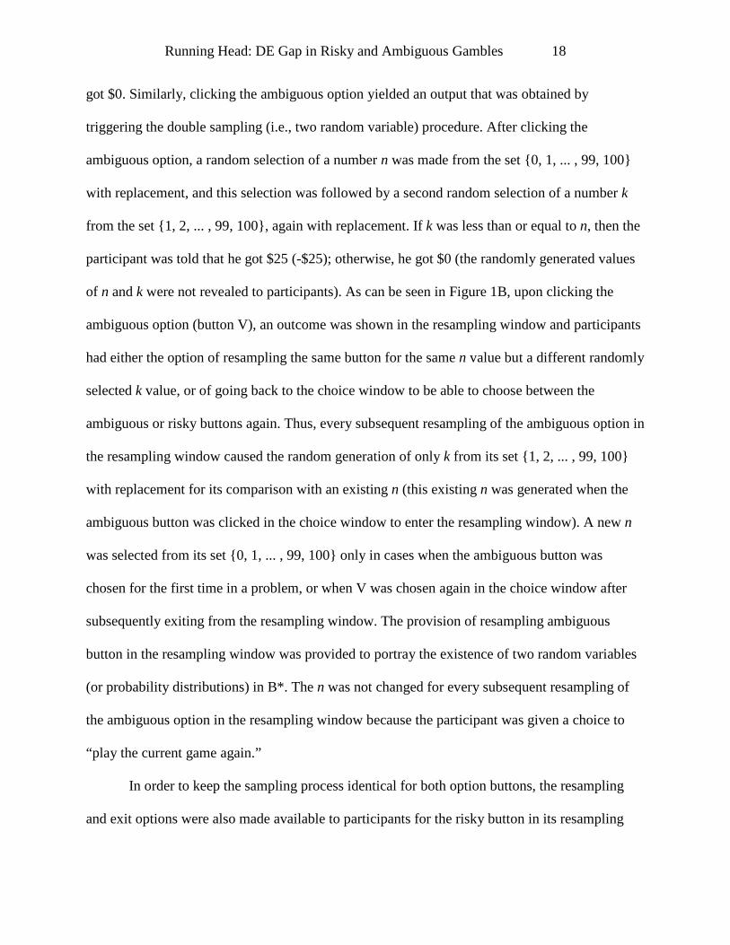
got $0. Similarly, clicking the ambiguous option yielded an output that was obtained by

triggering the double sampling (i.e., two random variable) procedure. After clicking the

ambiguous option, a random selection of a number n was made from the set {0, 1, ... , 99, 100}

with replacement, and this selection was followed by a second random selection of a number k

from the set {1, 2, ... , 99, 100}, again with replacement. If k was less than or equal to n, then the

participant was told that he got $25 (-$25); otherwise, he got $0 (the randomly generated values

of n and k were not revealed to participants). As can be seen in Figure 1B, upon clicking the

ambiguous option (button V), an outcome was shown in the resampling window and participants

had either the option of resampling the same button for the same n value but a different randomly

selected k value, or of going back to the choice window to be able to choose between the

ambiguous or risky buttons again. Thus, every subsequent resampling of the ambiguous option in

the resampling window caused the random generation of only k from its set {1, 2, ... , 99, 100}

with replacement for its comparison with an existing n (this existing n was generated when the

ambiguous button was clicked in the choice window to enter the resampling window). A new n

was selected from its set {0, 1, ... , 99, 100} only in cases when the ambiguous button was

chosen for the first time in a problem, or when V was chosen again in the choice window after

subsequently exiting from the resampling window. The provision of resampling ambiguous

button in the resampling window was provided to portray the existence of two random variables

(or probability distributions) in B*. The n was not changed for every subsequent resampling of

the ambiguous option in the resampling window because the participant was given a choice to

“play the current game again.”

In order to keep the sampling process identical for both option buttons, the resampling

and exit options were also made available to participants for the risky button in its resampling

Running Head: DE Gap in Risky and Ambiguous Gambles 19

window. In the case of the risky button, every subsequent resampling of this button without

choosing to exit from the resampling window caused a new m to be randomly generated from its

set {1, 2, ... , 99, 100} with replacement and then this m was compared with 50 to generate an

outcome (the randomly generated value of m was not revealed to participants). Therefore, the

process of generating m in the risky option was the same whether this option was chosen for the

first time in a problem, whether this option was sampled again after exiting from the resampling

window, or whether this option was resampled without exiting from the resampling window.

Once participants were satisfied with their sampling, they gave their final choice for one

of the two option buttons by clicking on the “Play for Real” button followed their choice. As

shown in Figure 1B, the “Play for Real” button was located in the choice window, so if a

participant was in the resampling window, then she needed to exit from that window to be able to

make a final choice. Like in the description condition, they were asked to choose one of the

button options among strict preference, indifference preference, and in-between preference in a

following window after submitting their final choice in each problem. Just like in description, for

a problem, we treat the proportion of ambiguous button choices as a measure of ambiguity-

seeking behavior. Although participants were told about the differences between the risky and

ambiguous options through instructions before starting their experiment, they might not perceive

any difference between these two options based upon their sampling (as the actual sampling

process and the generation of random numbers was kept hidden from participants under both

options in experience). Thus, keeping the three preference strengths allows us to account for any

differences that our participants might perceive between the two options in the experience

condition.

----------------------------------INSERT FIGURE 1A, B ABOUT HERE------------------------------

Running Head: DE Gap in Risky and Ambiguous Gambles 20

Procedure

Participants were randomly assigned to one of the two conditions, experience or

description. Within each condition they were given two problems, gain and loss, in a random

order. Participants read the instructions about the task and how they would be paid. Questions

were answered at the time they read these instructions, but none were answered while

participants performed the problems. In the experience condition, participants did not know

about the random numbers being generated behind the two buttons and they only saw the

resulting outcomes $25, $0 or -$25, depending upon the problem they were playing. Participants

were shown their final choices’ outcomes in each problem only after they finished playing both

problems. Participants’ earnings were scaled, they were handed their base and performance

payments, and thanked for their participation.

Results

Table 1 shows the proportion of ambiguity-seeking choices for the different preference

strengths in the experience and description conditions for both loss and gain problems,

respectively. In experience, there were 43 participants who expressed a strict preference for one

of the two options (47%); 33 participants who expressed indifferences between the two options

(36%); and, 16 participants who expressed strength of preferences in-between a strict preference

and an indifference (17%). In the description condition, there were 29 participants who

expressed a strict preference for one of the two options (48%); 21 participants who expressed

indifferences between the two options (34%); and, 11 participants who expressed strength of

preferences in-between a strict preference and an indifference (18%). Thus, across the

description and experience conditions, the proportion of participants expressing the different

Running Head: DE Gap in Risky and Ambiguous Gambles 21

preference strengths was similar. This result shows that participants perceived the two options,

risky and ambiguous, similarly across the experience and description conditions.

Furthermore, as shown in the table, there exists a DE gap for strict preferences in both the

gain and loss problems. The nature of the gap and its valence in both gain and loss problems is

according to expectations stated in H1 and H2: A greater proportion of choices are ambiguity-

seeking in experience compared with in description, and this effect is similar in gain and loss

problems. Furthermore, there is an absence of a gap among people who did not have a strict

preference for their final choice (i.e., those with indifference or in-between preferences). Thus,

people who did not perceive differences between options based upon their sampling exhibited

similar preferences across the description and experience conditions. Overall, these results are in

agreement with our expectation of a DE gap existing in decisions under ambiguity.

----------------------------------INSERT TABLE 1 ABOUT HERE------------------------------

Sampling behavior. Given that the DE gap under ambiguity is similar to a gap under

risk, we expect that the psychological mechanisms under risk would also be relevant for

decisions under ambiguity. Based upon predictions from the IBL model and decisions from

experience literature, we expected reliance on small samples, frequency, and recency to be the

driving psychological mechanisms of the behavior in the experience condition of our experiment

(Gonzalez & Dutt, 2011; Hertwig & Erev, 2009). Here, we systematically investigate these

psychological mechanisms by analyzing the sampling behavior from participants in the

experience condition.

Sample size. In experiential decisions under risk, the leading cognitive explanation of the

DE gap has been a “reliance on small samples” (Hertwig & Erev, 2009). Across a number of

studies, participants have sampled options relatively few times (median number of samples often

Running Head: DE Gap in Risky and Ambiguous Gambles 22

vary between 11 and 19) (Hau et al., 2008; Hertwig & Erev, 2009). In our experiment, the

median number of samples was 20 in the loss problem and 26 in the gain problem. These

numbers of samples are larger than those found in decisions under risk experiments. This finding

might be due to the dynamics of the probabilities that participants encountered with our

experimental paradigm. In our experiment, based upon the first random variable in the

ambiguous option, participants may encounter problems of different probabilities across their

sampling; some may involve rare outcomes and frequent outcomes in one single sampling of the

ambiguous button. That is unlike decisions under risk, where the probability of the risky option

remains fixed across samples and one expects to observe outcomes consistently with this fixed

probability. It is possible that given the consistency of the probabilities in decisions under risk,

people might be satisfied with their samples sooner.

Frequency and Recency of Experienced Outcomes. Gonzalez and Dutt (2011), Hertwig

et al. (2004), and Weber (2006) documented that participants’ final choices (i.e., post sampling)

were a function of the recency and frequency of experienced outcomes during sampling in

experiential decisions under risk. The reliance on recency and frequency of experienced

outcomes follows directly from IBLT (Gonzalez et al., 2003).

In order to understand the role of frequency of experienced outcomes in our dataset, we

analyzed the proportion of ambiguity-seeking final choices among participants who encountered

the non-zero outcome ($25 or -$25) more or less frequently than expected during sampling of the

ambiguous option (the latter being determined by the probabilities in the problems encountered

during sampling). Table 2 (A) shows this frequency analysis for different problems and

preference strengths. In the gain problem, the proportion of ambiguity-seeking choices was

higher for those who saw $25 as or more frequently than expected compared with those who saw

Running Head: DE Gap in Risky and Ambiguous Gambles 23

$25 less frequently than expected for both indifference and strict preferences. A similar but

reversed pattern for the loss problem was found: The proportion of ambiguity-seeking

preferences was lower for those that saw -$25 as or more frequently than expected compared

with those who saw -$25 less frequently than expected (88%) for both indifferent and strict

preferences. In the case of in-between preferences, this pattern was weaker in both the gain and

loss problems (in fact there are very few data points to conclude either way). These findings

taken together reveal that frequency of experienced outcomes did influence participants’ final

choices in both problems.

We also analyzed participants’ sampling for the role of recency in their final choices

using the method suggested in Hertwig et al. (2004). For this analysis, we split the sequence of

draws (samples) from each option into two halves for each problem and each participant giving

different preference strengths. Then, we computed the options’ average payoffs obtained for the

first and second halves of the samples, predicted each person’s choice on the basis of the average

payoffs (the option with the higher average payoff was predicted to be chosen), and analyzed

how many of the actual final choices coincided with the predicted choices. If recency plays a role

in decisions from ambiguity (as suggested by IBLT), then the second half of samples should

predict a greater proportion of actual choices compared with the first half of samples. Table 2 (B)

shows the analysis of recency for different problems and preference strengths. Overall, the

proportion of actual choices correctly predicted by the first or second sample halves show small

effects of recency: The second half of samples explained 50% of actual choices; whereas the first

half of samples explained 48% of the same choices. The effects of recency were particularly

stronger in gain problems for strict and in-between preferences and for in-between preferences in

loss problems. However, recency did not play a role for strict preferences in the loss problem,

Running Head: DE Gap in Risky and Ambiguous Gambles 24

and for indifference preferences in the loss and gain problems. Overall, these results show a lack

of systematic pattern for recency’s role across problems and preference strengths. In fact, like in

our experiment, the role of recency in explaining final choices has not been consistently found.

Unlike Gonzalez and Dutt (2011), Hertwig et al. (2004), and Weber (2006); Hau et al. (2008)

and Rakow, Demes, and Newell (2008) found its impact on final choices to be quite limited.

Even Gonzalez and Dutt (2011), who used different datasets for their analyses, found that the

recency’s role was not consistent across all datasets.

----------------------------------INSERT TABLE 2 A, B ABOUT HERE------------------------------

General Discussion

We found a DE gap for decisions under ambiguity. When people are simultaneously

presented with risky and ambiguous options people are ambiguity-averse in description (as has

been classically documented in ambiguity literature by Ellsberg, 1961 and others), while they are

ambiguity-seeking in experience. The DE gap appears for people who express a strict preference

for their final choice and it is weaker for those that express an indifference preference or an in-

between preference. This latter finding is reasonable considering the fact that people who exhibit

a strict preference are likely those that are able to distinguish between the two options, risky and

ambiguous, based upon their sampling of outcomes (in experience) or based upon the descriptive

ambiguity of the random variables in description. From an IBL perspective, the DE gap for

participants expressing a strict preference is revealed in the effects of frequency for these

participants. When these participants see $25 in the ambiguous option as or more frequently than

expected, a greater proportion choose it at final choice compared to those that see it less

frequently than expected. However, when these participants see -$25 in the ambiguous option as

or more frequently than expected, a smaller proportion choose it at final choice compared to

Running Head: DE Gap in Risky and Ambiguous Gambles 25

those that see it less frequently than expected. In addition, the DE gap for participants with a

strict preference is also exhibited by the role of recency in the gain problem: A greater proportion

of final choices seem to agree with the second sample half compared to the first sample half.

However, similar recency effects were weaker for the loss problem. We can only speculate, but

perhaps, the negative (-$25) outcome is more salient when it occurs in the first half of samples

compared to when it occurs in the second half of samples. This saliency of early negative

outcomes is consistent with hyperbolic discounting literature (Thaler, 1981), where early losses

are more impacting and painful compared to delayed losses.

Furthermore, although decisions under risk and ambiguity seem similar and both these

decisions involve similar cognitive processes as suggest by IBLT, there are important differences

between the ambiguous experiential decisions (as in our experiment) and those under risk. In

experiential decisions under ambiguity, the frequency of the ambiguous option’s outcomes

changes stochastically across samples (due to the two random variables involved). Therefore, the

experienced frequency of outcomes for the ambiguous option is essentially unknown to the

participants, and the likelihood of different outcomes cannot be expressed with any mathematical

precision across samples. However, in experiential decisions under risk, the frequency of

observed outcomes for an option remains the same and can be expressed with mathematical

precision. Perhaps, it is due to these differences between risk and ambiguity that we find some

peculiarities in human sampling behavior in our experiment. For example, although the observed

median sample size in our experiment was small; this median sample size was larger than that of

decisions under risk (Hertwig et al. 2004).

Despite these differences, we also found overlaps between our results and those known

for experiential decisions under risk. For example, the influence of recency on participants’

Running Head: DE Gap in Risky and Ambiguous Gambles 26

choices in decisions under risk has been somewhat inconsistent and our results for decisions

under ambiguity seem to agree with this inconsistency: Recency had little role to play in our

results as the first and second half of samples seem to explain the final choices equally well in

both gain and loss problems. Given that recency is an integral part of IBLT and its role is

inconsistent, it seems that frequency is a stronger driving mechanism compared to recency to

explain final choices based upon sampling.

Our results on the consistency of the DE gap in experiential decisions under ambiguity

support similar findings in experiential decisions under risk (e.g., Hertwig et al., 2004; Hertwig

& Erev, 2009). For decisions under ambiguity, people are ambiguity-averse only when decisions

are made from description, and they become ambiguity-seeking when decisions are made from

experience. One plausible reason for this finding could be that, in experience, participants are

unable to perceive the complexity of two random variables in the ambiguous option during their

sampling and this causes them to prefer the ambiguous option. However, in description,

participants get to read the description of the extra random variable and the complexity of the

random process makes them move away from the ambiguous option. In fact, an extra random

variable in the ambiguous option compared to the risky option is sufficient to observe a gap

between choices in description and experience. This observation is the main contribution of our

experiment.

In addition, as shown in our results, participants choose the option that gives them the

high payoff more frequently than expected in the experience condition. This observation would

suggest that a second factor for the DE gap observed in our study is sampling error (Hau et al.,

2010; Ungemach et al., 2009). Thus, in the near future, we plan to do an additional study where

one reduces or eliminate sampling error either via increased sample sizes (e.g., Hau et al., 2010)

Running Head: DE Gap in Risky and Ambiguous Gambles 27

or via a constrained-sampling technique (Ungemach et al., 2009). In general, future research is

likely to benefit by drawing upon the documented similarities and differences for experiential

decisions under risk and under ambiguity, and in further investigating the reasons for the

presence of a DE gap in decisions under ambiguity due to ambiguity differences created in other

possible ways.

Running Head: DE Gap in Risky and Ambiguous Gambles 28

References

Abdellaoui, M., Vossmann, F., & Weber, M. (2005). Choice-based elicitation and

decomposition of decision weights for gains and losses under uncertainty. Management

Science, 51, 1384–1399. doi: 10.1287/mnsc.1050.0388

Arló-Costa, H., Dutt, V., Gonzalez, C., & Helzner, J. (2011). The description/experience gap in

the case of uncertainty. In F. Coolen, G. de Cooman, T. Fetz, & M. Oberguggenberger

(Eds.), Proceedings of the Seventh International Symposium on Imprecise Probability:

Theories and Applications (pp. 31-39). Innsbruck, Austria: SIPTA.

Arló-Costa, H., & Helzner, J. (2005). Comparative ignorance and the Ellsberg phenomenon. In

F. Cozman, R. Nau, & T. Seidenfeld (Eds.), Proceedings of the Fourth International

Symposium on Imprecise Probabilities and Their Applications. Pittsburgh, PA: SIPTA.

Arló-Costa, H., & Helzner, J. (2007). On the explanatory value of indeterminate probabilities. In

G. De Cooman, J. Vejnarova, & M. Zaffalon (Eds.), Proceedings of the Fifth

International Symposium on Imprecise Probabilities and Their Applications (pp. 117-

125). Prague, Czech Republic: SIPTA.

Arló-Costa, H., & Helzner, J. (2009). Iterated random selection as intermediate between risk and

uncertainty. In T. Augustin, F. P. A. Coolen, S. Moral, & M. C. M. Troaes (Eds.),

Proceedings of the Sixth International Symposium on Imprecise Probabilities and Their

Applications (pp. 1-9). Durham, UK: SIPTA.

Camerer, C., & Weber, M. (1992). Recent developments in modeling preferences: Uncertainty

and ambiguity. Journal of Risk and Uncertainty, 5(4), 325 -370. doi:

10.1007/BF00122575

Running Head: DE Gap in Risky and Ambiguous Gambles 29

Chakravarty, S. & Roy, J. (2009). Recursive expected utility and the separation of attitudes

towards risk and ambiguity: An experimental study. Theory and Decision, 66(3), 199–

228. doi: 10.1007/s11238-008-9112-4

Chow, C. & Sarin, R. (2002). Known, unknown and unknowable uncertainties. Theory and

Decision, 52(2), 127-138. doi: 10.1023/A:1015544715608

Cohen, M., Jaffray, J. Y., & Said, T. (1987). Experimental comparisons of individual behavior

under risk and under uncertainty for gains and for losses. Organizational Behavior and

Human Decision Processes, 39(1), 1–22. doi: 10.1016/0749-5978(87)90043-4

Curley, S. P., & Yates, J. F. (1989). An empirical evaluation of descriptive models of ambiguity

reactions in choice situations. Journal of Mathematical Psychology, 33(4), 397–427. doi:

10.1016/0022-2496(89)90019-9

Davidovich, L. & Yassour, Y. (2009). Ambiguity preference. Emek Hefer, Israel: Ruppin

Academic Center.

Di Mauro, C., & Maffioletti, A. (1996). An experimental investigation of the impact of

ambiguity on the valuation of self-insurance and self-protection. Journal of Risk and

Uncertainty, 13(1), 53–71. doi: 10.1007/BF00055338

Dobbs, I. M. (1991). A Bayesian approach to decision-making under ambiguity. Economica,

58(232), 417–440. doi: 10.2307/2554690

Du, N., & Budescu, D. (2005). The effects of imprecise probabilities and outcomes in

evaluating investment options. Management Science, 51(12), 1791-1803.

Dutt, V., & Gonzalez, C. (2012). Why do we want to delay actions on climate change? Effects of

probability and timing of climate consequences. Journal of Behavioral Decision Making,

25(2), 154–164. doi: 10.1002/bdm.721

Running Head: DE Gap in Risky and Ambiguous Gambles 30

Einhorn, H. J., & Hogarth, R. M. (1986). Decision making under ambiguity. Journal of

Business, 59(4), S225–S250.

Ellsberg, D. (1961). Risk, ambiguity, and the savage axioms. Quarterly Journal of Economics

75(4), 643-669. doi: 10.2307/1884324

Fox, C. R., & Hadar, L. (2006). "Decisions from experience" = sampling error + prospect theory:

Reconsidering Hertwig, Barron, Weber & Erev (2004). Judgment and Decision Making,

1(2), 159-161.

Gonzalez, C., & Dutt, V. (2011). Instance-Based Learning: Integrating sampling and repeated

decisions from experience. Psychological Review, 118(4), 523-551. doi:

10.1037/a0024558

Gonzalez, C., Lerch, F. J., & Lebiere, C. (2003). Instance-based learning in real-time dynamic

decision making. Cognitive Science, 27(4), 591-635. doi: 10.1016/S0364-0213(03)00031-

4

Guney, S., & Newell, B. R. (2011). The Ellsberg ‘problem’ and implicit assumptions under

ambiguity. In L. Carlson, C. Hoelscher, & T. F. Shipley (Eds.), Proceedings of the 33rd

Annual Meeting of the Cognitive Science Society (pp. 2323-2328). Austin, TX: Cognitive

Science Society.

Hadar, L., & Fox, C. R. (2009). Information asymmetry in decision from description versus

decision from experience. Judgment and Decision Making, 4(4), 317–325.

Halevy, Y. (2007). Ellsberg revisited: An experimental study. Econometrica, 75(2), 503-536.

doi: 10.1111/j.1468-0262.2006.00755.x

Running Head: DE Gap in Risky and Ambiguous Gambles 31

Hau, R., Pleskac, T. J., Kiefer, J., & Hertwig, R. (2008). The description-experience gap in risky

choice: The role of sample size and experienced probabilities. Journal of Behavioral

Decision Making, 21(5), 493-518. doi: 10.1002/bdm.598

Hau, R., Pleskac, T. J., & Hertwig, R. (2010). Decisions From Experience and Statistical

Probabilities: Why They Trigger Different Choices Than a Priori Probabilities. Journal of

Behavioral Decision Making, 23(1), 48-68. doi: 10.1002/bdm.665

Hertwig, R. (in press). The psychology and rationality of decisions from experience. Synthese.

doi: 10.1007/s11229-011-0024-4

Hertwig, R., Barron, G., Weber, E. U., & Erev, I. (2004). Decisions from experience and the

effect of rare events in risky choice. Psychological Science, 15(8), 534-539. doi:

10.1111/j.0956-7976.2004.00715.x

Hertwig, R., & Erev, I. (2009). The description-experience gap in risky choice. Trends in

Cognitive Sciences, 13(12), 517-523. doi: 10.1016/j.tics.2009.09.004

Ho, J. L. Y., Keller, L. R., & Keltyka, P. (2002). Effects of outcome and probabilistic ambiguity

on managerial choices. Journal of Risk and Uncertainty, 24(1), 47–74. doi:

10.1023/A:1013277310399

Hogarth, R. M., & Kunreuther, H. (1989). Risk, ambiguity, and insurance. Journal of Risk and

Uncertainty, 2(1), 5-35. doi: 10.1007/BF00055709

Keren, G. B., & Gerritsen, L. E. M. (1999). On the robustness and possible accounts of

ambiguity aversion. Acta Psychologica, 103(1-2), 149–172. doi: 10.1016/S0001-

6918(99)00034-7

Knight, F. H. (1921). Risk, uncertainty and profit. Boston: Houghton Mifflin.

Running Head: DE Gap in Risky and Ambiguous Gambles 32

Luce, R. D. & Raiffa, H. (1957). Games and decisions: Introduction and critical survey. Dover,

NY: Wiley.

Mangelsdorff, L., & Weber, M. (1994). Testing choquet expected utility. Journal of

Economic Behavior and Organization, 25(3), 437–457. doi: 10.1016/0167-

2681(94)90109-0

Rakow, T., Demes, K., & Newell, B. (2008). Biased samples not mode of presentation:

Reexamining the apparent underweighting of rare events in experience-based choice.

Organizational Behavior and Human Decision Processes, 106(2), 168–179. doi:

10.1016/j.obhdp.2008.02.001

Rakow, T., & Newell, B. R. (2010). Degrees of uncertainty: An overview and framework for

future research on experience-based choice. Journal of Behavioral Decision Making,

23(1), 1-14. doi: 10.1002/bdm.681

Thaler, R. H. (1981). Some Empirical Evidence on Dynamic Inconsistency. Economic Letters,

8(3), 201–207. doi:10.1016/0165-1765(81)90067-7

Tversky, A., & Fox, C. R. (1995). Weighing risk and uncertainty. Psychological Review, 102(2),

269-283. doi: 10.1037/0033-295X.102.2.269

Ungemach, C., Chater, N., & Stewart, N. (2009). Are Probabilities Overweighted or

Underweighted When Rare Outcomes Are Experienced (Rarely)? Psychological Science,

20(4), 473-479. doi: 10.1111/j.1467-9280.2009.02319.x

Viscusi, W. K., & Chesson, H. (1999). Hopes and fears: The conflicting effects of risk

ambiguity. Theory and Decision, 47(2), 157-184. doi: 10.1023/A:1005173013606

Wakker, P. P. (2010). Prospect theory for risk and ambiguity. Cambridge, UK: Cambridge

University Press.

Running Head: DE Gap in Risky and Ambiguous Gambles 33

Weber, E. U. (2006). Experience based and description based perceptions of long term risk: Why

global-warming does not scare us (yet). Climatic Change, 77(1-2), 103–120. doi:

10.1007/s10584-006-9060-3

Weber, E. U., Shafir, S., & Blais, A.-R. (2004). Predicting risk sensitivity in humans and lower

animals: Risk as variance or coefficient of variation. Psychological Review, 111(2), 430–

445. doi: 10.1037/0033-295X.111.2.430

Weber, E. U., & Johnson, E. J. (2008). Decisions under uncertainty: Psychological, economic,

and neuroeconomic explanations of risk preference. In P. Glimcher, C. Camerer, E. Fehr,

& R. Poldrack (Eds.), Neuroeconomics: Decision making and the brain (pp. 127-144).

New York: Elsevier.

Yates, J. F., & Zukowski, L.G. (1976). Characterization of ambiguity in decision making.

Behavioral Science, 21(1), 19-25. doi: 10.1002/bs.3830210104

Running Head: DE Gap in Risky and Ambiguous Gambles 34

Table 1 Proportion of ambiguity-seeking choices for different preference strengths in the experience and description conditions for the loss and gain problems.

Gain Problem Preference Strength1 Experience Description Description – Experience Gap

Indifferent 42% (14/33) 48% (10/21) -06% (Z=-0.371, ns, r = -0.04) Strict 65% (28/43) 38% (11/29) +27% (Z=-2.255, p < .05, r2 = -0.27)

In-between 44% (07/16) 55% (06/11) -11% (Z=-0.541, ns, r = -0.10) Loss Problem

Preference Strength Experience Description Description – Experience Gap Indifferent 63% (22/35) 53% (08/15) +10% (Z=-0.624, ns, r = -0.09)

Strict 66% (27/41) 41% (14/34) +25% (Z=-2.123, p < .05, r = -0.25) In-between 44% (07/16) 58% (07/12) -14% (Z=-0.750, ns, r = -0.14)

Note. The bolded text indicates results that are significant at p < .05. 1 Preference strengths account for any perceived difference between the ambiguous and risky options after a choice is made for one of them. 2The r is the effect size.

Running Head: DESCRIPTION EXPERIENCE GAP UNDER UNCERTAINTY 35

Table 2 (A) The proportion of ambiguity-seeking final choices based upon the frequency of observing $25 or -$25 in the ambiguous option during sampling for different problems and preference strengths.

Gain Problem Preference Strength Proportion of ambiguous option final choices

Observed $25 on ambiguous option as or more frequently than

expected during sampling

Observed $25 on ambiguous option always

less frequently than expected during sampling

Indifferent 52% (13/25) 0% (0/6) Strict 81% (22/27) 45% (5/11)

In-between 50% (4/8) 60% (3/5) Loss Problem

Preference Strength Proportion of ambiguous option final choices

Observed -$25 on ambiguous option as or more frequently than

expected during sampling

Observed -$25 on ambiguous option always

less frequently than expected during sampling

Indifferent 60% (18/30) 100% (3/3) Strict 59% (19/32) 88% (7/8)

In-between 50% (6/12) 33% (1/3) Table 2 (B) The proportion of actual choices correctly predicted based upon first or second half of sampling for different problems and preference strengths.

Gain Problem Preference Strength Proportion of actual choices correctly predicted

by first-half samples by second-half samples Indifferent 59% (19/32) 44% (14/32)

Strict 31% (12/39) 51% (20/39) In-between 33% (4/12) 42% (5/12)

Loss Problem Preference Strength Proportion of actual choices correctly predicted

Sampling first half Sampling second half Indifferent 52% (17/33) 48% (16/33)

Strict 55% (22/40) 48% (19/40) In-between 53% (8/15) 80% (12/15)

Overall

(across different preference strengths and

problems)

48% (82/171) 50% (86/171)

Running Head: DESCRIPTION EXPERIENCE GAP UNDER UNCERTAINTY 36

(A)

(B)

Choice Window Resampling Window

Figure 1. (A) The gain problem in the description condition. Participants had to choose one of the two options (games), one time, by clicking on one of the two buttons. (B). The gain problem in the experience condition. Option V is ambiguous (B*) and option C is risky (A). During sampling, a participant clicks button V (choice window) and is shown the outcome ($25) (resampling window). The participant has now the option to either resample V (by clicking on “Play the current game again”), or exit from this window (participants exited the resampling window by clicking on the button labeled “Return to the top level of the sampling phase”). To make a final choice, participants had to click the “play for real” button followed by their final choice. Sampling of options did not cost any money, only the final choice affected earnings.