The DeterminantsofBrazil's RecentRapid Declinein Fertility

NeE COpyRY USE ON-LV

REPORT 0.23

COMMITTEE ONPOPULAnON AND DEMOGRAPHY

The DeterminantsofBrazil's RecentRapid Declinein Fertility

Thomas W. MerrickFlza Berquo

Report No. 23

Panel on Fertility DeterminantsCommittee on Population and DemographyCommission on Behavioral and

Social Sciences and EducationNational Research Council

NAS-NAE

OCT ~ 1 1983

LIBRARYNA TIONAL ACADEMY PRESSWashington, D.C. 1983

8" ~ - 0 J:)25

C· J

HOTICE: The project that is the sUbject of this reportwas approved by the Governing Board of the HationalResearch Council, whose members are drawn from thecouncils of the Hational Academy of Sciences, theHational Academy of Engineering, and the Institute ofMedicine. The members of the committee responsible forthe report were chosen for their special competences andwith regard for appropriate balance.

This report has been reviewed by a group other thanthe authors according to procedures approved by a ReportReview Committee consisting of members of the HationalAcademy of Sciences, the Hational Academy of Engineering,and the Institute of Medicine.

The Hational Research Council was established by theHational Academy of Sciences in 1916 to associate thebroad community of science and technology with theAcademy's purposes of furthering knowledge and ofadvising the federal government. The Council operates inaccordance with general policies determined by theAcademy under the authority of its congressional charterof 1863, which establishes the Academy as a private,nonprofit, self-governing membership corporation. TheCouncil has become the principal operating agency of bOththe Hational Academy of Sciences and the Hational Academyof Engineering in the conduct of their services to thegovernment, the pUblic, and the scientific andengineering communities. It is administered jointly bybOth Academies and the Institute of Medicine. TheHational Academy of Engineering and the Institute ofMedicine were established in 1964 and 1970, respectively,under the charter of the Hational Academy of Sciences.

Available from

HATIOIIAL ACADBMY PRESS2101 COnstitution Avenue, H.W.Washington, D.C. 20418

Printed in the United States of America

PANEL ON FERTILITY DETERMINANTS

W. PARKER MAULDIN (Chair), The Rockefeller Foundation,New York

ELZA BERQUO, Centro Brasileiro de Analise e planejamento,Sao Paulo, Brazil

WILLIAM BRASS, Centre for population Studies, LondonSchool of Hygiene and Tropical Medicine

DAVID R. BRILLINGER, Department of Statistics, Universityof California, Berkeley

V.C. CHIDAMBARAM, World Fertility Survey, LondonJULIE DAVANZO, Rand Corporation, Santa MonicaRICHARD A. EASTERLIN, Department of Economics, University

of Southern California, Los AngelesJAMES T. FAWCETT, East-West Population Institute,

East-West Center, HonoluluRONALD FREEDMAN, Population Studies Center, University of

MichiganDAVID GOLDBERG, PopUlation Studies Center, University of

MichiganRONALD GRAY, School of Hygiene and Public Health, The

Johns Hopkins University, BaltimorePAULA E. HOLLERBACH, Center for Policy Studies, The

PopUlation Council, New YorkRONALD LEE, Graduate Group in Demography, University of

California, BerkeleyROBERT A. LEVINE, Graduate School of Education, Harvard

UniversitySUSAN C.M. SCRIMSHAW, School of Public Health, university

of California, Los AngelesROBERT WILLIS, Department of Economics, State University

of New York, Stony Brook

ROBERT J. LAPHAM, StUdy Director

iii

CCMtITTBE ON POPULATION AND DEMOGRAPHY

ANSLEY J. COIUoE (Chair), Office of population Research,Princeton University

WILLIAM BRASS, Centre for Population Studies, LondonSchool of Hygiene and Tropical Medicine

LEE-JAY CHO, East-West population Institute, East-WestCenter, Honolulu

RONALD FREEDMAN, Population Studies Center, university ofMichigan

NATHAN KBYl"ITZ, Department of Sociology, HarvardUniversity

LESLIE KISH, Institute for Social Research, university ofMichigan

W. PARKER MAULDIN, Population Division, The RockefellerFoundation, New York

JANE MENKEN, Office of Population Research, PrincetonUniversity

SAMUEL PRESTON, Population Studies Center, university ofPennsylvania

WILLIAM SELTZER, Statistical Office, United NationsCONRAD TABUBER, Kennedy Institute, Center for Population

Research, Georgetown UniversityETIENNE VAN DE HALLE, Population Studies Center,

University of Pennsylvania

ROBERT J. LAPHAM, Study Director

NOTE: Members of the Committee and its panels andworking groups participated in this project in theirindividual capacities, the listing of theirorganizational affiliation is for identification purposesonly, and the views and designations used in this reportare not necessarily those of the organizations mentioned.

iv

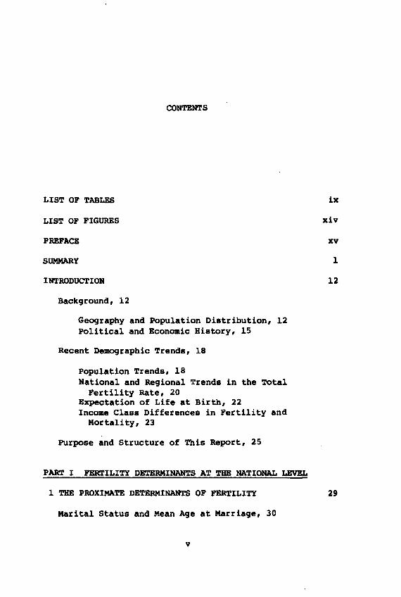
CONTENTS

LIST OF TABLES

LIST OF FIGURES

PREFACE

SUMMARY

INTRODUCTION

Background, 12

Geography and Population Distribution, 12Political and Economic History, lS

Recent Demographic Trends, 18

Population Trends, 18National and Regional Trends in the Total

Fertility Rate, 20Expectation of Life at Birth, 22Income Class Differences in Fertility and

Mortality, 23

Purpose and Structure of This Report, 2S

PART I FERTILITY DETERMINANTS AT THE NATIONAL LEVEL

1 THE PROXIMATE DETERMINANTS OF FERTILITY

Marital Status and Mean Age at Marriage, 30

v

ix

xiv

xv

1

12

29

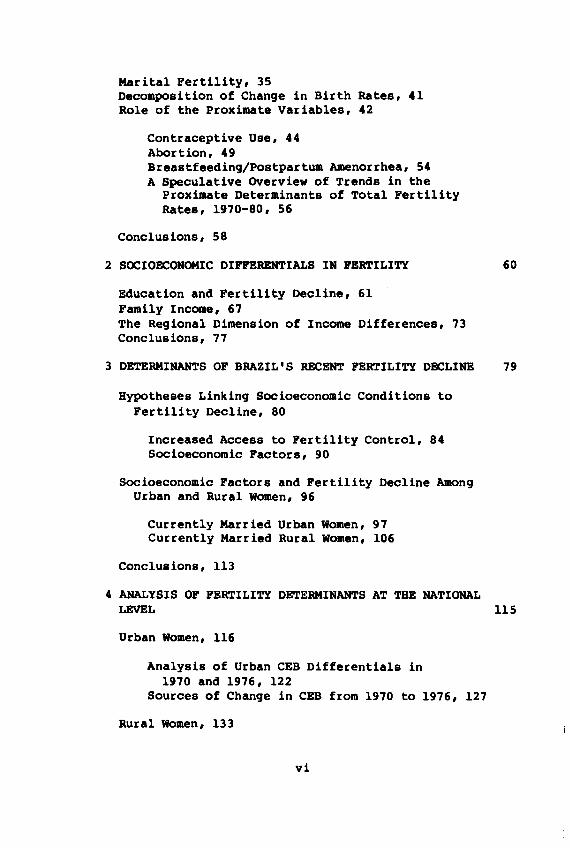
Marital Fertility, 35Decomposition of Change in Birth Rates, 41Role of the Proximate Variables, 42

Contraceptive Use, 44Abortion, 49Breastfeeding/Postpartum Amenorrhea, 54A Speculative Overview of Trends in the

Proximate Determinants of Total FertilityRates, 1970-80, 56

Conclusions, 58

2 SOCIOECONOMIC DIFFERENTIALS IN FERTILITY

Education and Fertility Decline, 61Family Income, 67The Regional Dimension of Income Differences, 73Conclusions, 77

60

3 DETERMINANTS OF BRAZIL'S RECENT FERTILITY DECLINE 79

Hypotheses Linking Socioeconomic Conditions toFertility Decline, 80

Increased Access to Fertility Control, 84Socioeconomic Factors, 90

Socioeconomic Factors and Fertility Decline AmongUrban and Rural Women, 96

Currently Married Urban Women, 97Currently Married Rural Women, 106

Conclusions, 113

4 ANALYSIS OF FERTILITY DETERMINANTS AT THE NATIONALLEVEL 115

Urban Women, 116

Analysis of Urban CEB Differentials in1970 and 1976, 122

Sources of Change in CEB from 1970 to 1976, 127

Rural Women, 133

vi

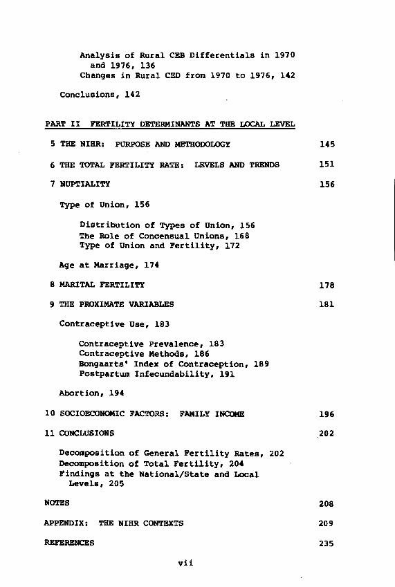
Analysis of Rural CEB Differentials in 1970and 1976, 136

Changes in Rural CED from 1970 to 1976, 142

Conclusions, 142

PART II FERTILITY DETERMINANTS AT THE LOCAL LEVEL

5 THE NIHR: PURPOSE AND METHODOLOGY 145

6 THE TOTAL FERTILITY RATE: LEVELS AND TRENDS 151

7 NUPTIALITY

Type of Union, 156

Distribution of TyPes of Union, 156The Role of Concensual Unions, 168TyPe of Union and Fertility, 172

Age at Marriage, 174

8 MARITAL FERTILITY

9 THE PROXIMATE VARIABLES

Contraceptive Use, 183

Contraceptive Prevalence, 183Contraceptive Methods, 186Bongaarts' Index of Contraception, 189Postpartum Infecundability, 191

Abortion, 194

10 SOCIOECONOMIC FACTORS: FAMILY INCOME

156

178

181

196

11 CONCLUSIONS .202

Decomposition of General Fertility Rates, 202Decomposition of Total Fertility, 204Findings at the National/State and Local

Levels, 205

NOTES 208

APPENDIX: THE NIHR CONTEXTS

REFERENCES

vii

209

235

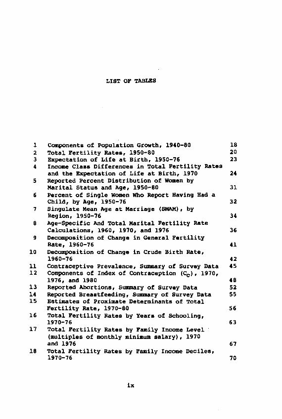
LIST OF TABLES

1 Components of Population Growth, 1940-80 182 Total Fertility Rates, 1950-80 203 Expectation of Life at Birth, 1950-76 234 Income Class Differences in Total Fertility Rates

and the EXPectation of Life at Birth, 1970 245 Reported Percent Distribution of Women by

Marital Status and Age, 1950-80 316 Percent of Single Women Who Report Having Had a

Child, by Age, 1950-76 327 Singulate Mean Age at Marriage (SHAM), by

Region, 1950-76 348 Age-Specific And Total Marital Fertility Rate

Calculations, 1960, 1970, and 1976 369 Decomposition of Change in General Fertility

Rate, 1960-76 4110 Decomposition of Change in Crude Birth Rate,

1960-76 4211 Contraceptive Prevalence, Summary of Survey Data 4512 Components of Index of Contraception (Cc )' 1970,

1976, and 1980 4813 Reported Abortions, Summary of Survey Data 5214 Reported Breastfeeding, Summary of Survey Data 5515 Estimates of Proximate Determinants of Total

Fertility Rate, 1970-805616 Total Fertility Rates by Years of Schooling,

1970-76 6317 Total Fertility Rates by Family Income Level

(multiples of monthly minimum salary), 1970and 1976 67

18 Total Fertility Rates by Family Income Deciles,1970-76 70

ix

19 Percent Distribution of All Women Aged 15-49 byIncome Deciles, Years in School, and Rural-UrbanResidence, 1970 and 1976 72

20 Unadjusted Total Fertility Rate by PNAD Regionand Income Decile, 1970 and 1976 74

21 Percent Distribution of Women Aged 15-49 by PNADRegion and Income Deciles, 1970 and 1976 75

22 Percent Distribution of Married Women Aged 15-44,by Contraceptive Use Status and Household Income 88

23 Contraceptive Prevalence Survey Data on Percentof currently Married WOmen Aged 15-44 UsingContraceptives, by Education 90

24 Source of Family Planning Supplies and Services,Currently Married Women Aged 15-44, CPS Data byState 91

25 Percent of Women Reported as Having No Schooling,by Age, 1960-80 93

26 Percent Distribution of All Women Aged 20-44 byAge and Years of Schooling, 1970 and 1976 94

27 Percent of Women Reported as Working, by Age andYears of Schooling, 1970 and 1976 95

28 Mean and Standard Error (S)a of Number ofChildren Ever Born, Currently Married UrbanWomen, by Age and Educational Attainment, 1970and 1976 97

29 Percent Working and Percent Migrants AmongCurrently Married, Urban Women, 1970 and 1976 99

30 Distribution of Currently Married Women Aged20-44 by OCcupation, Work Status, and Educa-tional Attainment, 1970 and 1976 101

31 Percent of Currently Married, Urban Women Livingin Households Reporting Ownership of a Tele-vision, by Age and Education, 1970 and 1976 102

32 Average Number of Children Ever Born for Cur-rently Married, Urban Women, by Age, Education,and Current Employment Status, 1970 and 1976 103

33 Average Number of Children Ever Born for Migrantand Nonmigrant Women, by Age and EducationalAttainment, 1970 and 1976 104

34 Mean Number of Children Ever Born for CurrentlyMarried, Rural Women by Region, EducationalAttainment, and Age, 1970 and 1976 108

35 Percent of Currently Married, Rural Women inProletarian Households, Percent Working, andPercent Migrant, by Age and Region, 1970 and1976 109

x

36 Mean Number of Children Ever Born for CurrentlyMarried, Rural Women Aged 20-44, by Region andProletarian Status, 1970 and 1976 111

37 Mean Number of Children Ever Born for CurrentlyMarried, Rural Women Aged 20-44, by Region andWOrk Status, 1970 and 1976 112

38 Variable Labels and Definitions, Urban Women 11839 Means (standard deviations) of Variables Used in

Analysis of Differences in Average Parity forUrban Women, 1970 and 1976 121

40 Regression Analysis, Average Number of ChildrenEver Born (CEB), Married Urban Women, 1970 124

41 Regression Analysis, Average Number of ChildrenEver Born (CEB), Married Urban Women, 1976 125

42 Changes in Contribution of Independent Variablesto Levels of CEB, 1970 and 1976 129

43 Regression Analysis and Test for Interactions,Merged 1970 and 1976 Data Files 130

44 Decomposition of Changes in Average Parity from1970 to 1976 Using Regression Coefficient forMerged Data 131

45 Percent of Women with GAP Greater than OneStandard Deviation from Mean, 1970 and 1976 133

46 Variable Labels and Definitions, Rural Women 13747 Means (standard deviations) of Variables Used in

Analysis of Differences in Average Parity forRural Women, 1970 and 1976 138

48 Regression Analysis, Average Number of ChildrenEver Born (CEB), Married Rural Women, 1970 140

49 Regression Analysis, Average Number of ChildrenEver Born (CES), Married Rural Women, 1976 141

50 Nine Contexts Defined in Terms of Modes of Produc­tion and Type of Involvement in the DevelopmentProcess 148

51 Total Fertility Rates, Nine Contexts, 1965,1970, and 1975 153

52 Mean Parity 1/2 (P25-29 + P30-34), 1965, 1970,and 1975 155

53 Percent Distribution of Ever-Married Women, byType of Marital Union, Nine Contexts, 1960,1970, and 1975 158

54 Percent Distribution of Ever-Married Women, byType of Marital Union, 1960, 1970, and 1978 160

55 Distribution of Unions According to Order andType 161

xi

56 Distribution of Ever-Married Women by Type ofFirst Union, for Three Marriage Cohorts:A (until 1960), B (1961-70), and C (1971-76),and for Nine Contexts 163

57 Distribution of Ever-Married Women by Type ofFirst Union, for Three Marriage Cohorts: A(until 1960), B (1961-70), and C (1971-76), andfor Pive Urban and Pour Rural Contexts 164

58 Distribution of Ever-Married women According toType of Pirst Union, for Three Marriage COhorts:A (until 1960), B (1961-70), and C (1971-76),Nine COntexts 166

59 ' Distribution of COnsensual Unions by DifferentTypes, Nine COntexts 170

60 Distribution of COnsensual Unions, by Type forThree Marriage COhorts, Recife 172

61 Mean Number of Children Ever Born Alive byEver-Married Women, by Type of Marital Union,Nine Contexts, 1975 173

62 Mean Number of Children Ever Born, for CurrentlyMarried Women (first marriage), by Type of Unionand Three Marriage COhorts, Nine COntexts 174

63 Estimates for Nuptiality Parameters UsingCoale's Method, Nine Contexts 175

64 Mean Age at Marriage (Bajnal method), NineCOntexts 176

65 Total Marital Pertility Rates, Nine COntexts,1970 and 1975 179

66 Values for the Pertility COntrol Measure (m)Estimated by Coale's Method, 1970 and 1975 180

67 Currently Married Women Aged 15-49 CurrentlyUsing COntraception, by Types of Methods, NineCOntexts 182

68 Currently Married Women Aged 15-49 CurrentlyUsing COntraception, Nine Contexts 184

69 Age Distribution of Currently Married,Sterilized Women Aged 15-49, Nine Contexts 187

70 Estimates (in percent) for Use Efficiency ofCOntraceptives (e), for Currently Married Women,Nine Contexts 190

71 Index of COntraception, Nine COntexts 19172 Percent of Breastfed Children at 4 Months of

Age, by Various Studies 19273 Values of wiw and Ci, Nine COntexts 19474 Total Abortion Rates (TAR) and Bongaarts'

Abortion Rate (Ca ), Nine Contexts 195

xii

75 Percent Distribution of Women Aged 15 and Over,by Per Capita Monthly Income (in fractions ofone minimum wage), Pive Urban Contexts, at Timeof Survey 197

76 Average Number of Children Born to Ever-MarriedWomen Aged 15 and Over, by Per Capita MonthlyIncome (in fractions of one minimum wage), PiveUrban Contexts 199

77 Changes in General Fertility Rates Due to AgeStructure, Marital Status, and MaritalFertility, Nine Contexts, 1970-75 203

78 Proximate Determinants of Total Fertility,Nine Contexts, 1975 206

A.1 Dynamics of the Population of Parnaiba(municipality) , 1940-70 214

A.2 DYnamics of the Population of Cachoeiro doItapemirim (municipality), 1940-70 217

A.3 Dynamics of the Population of Sao Jose dosCampos (municipality), 1940-70 221

A.4 Dynamics of the Population of Sertaozinho(municipality), 1940-70 228

A.5 Dynamics of the Population of Santa Cruz doSul (municipality), 1940-70 231

A.6 Dynamics of the Population of Recife(municipality), 1940-70 234

xiii

\

1

23

4

56

7

8

9

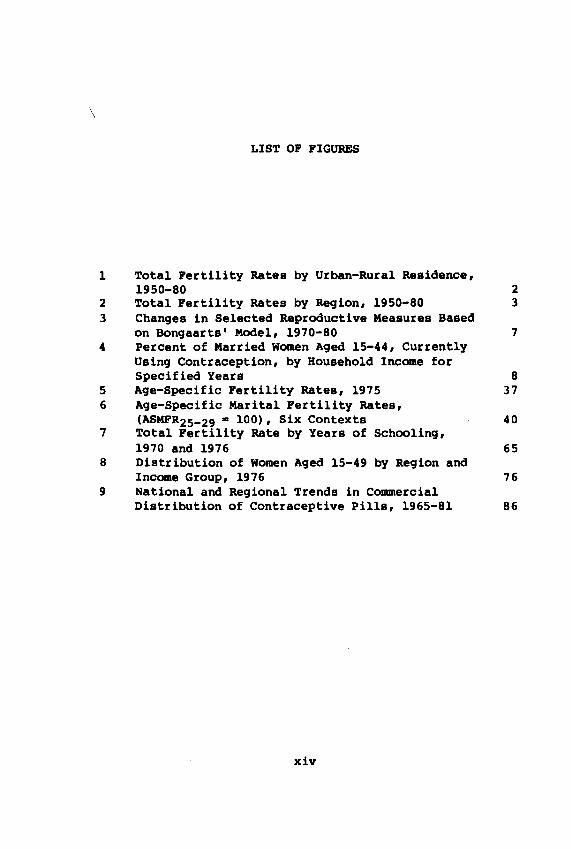
LIST OF FIGURES

Total Fertility Rates by Urban-Rural Residence,1950-80Total Fertility Rates by Region, 1950-80Changes in Selected Reproductive Measures Basedon Bongaarts' Model, 1970-80Percent of Married Women Aged 15-44, CurrentlyUsing Contraception, by Household Income forSpecified YearsAge-Specific Fertility Rates, 1975Age-Specific Marital Fertility Rates,(ASMPR25-29· 100), Six ContextsTotal Fertility Rate by Years of Schooling,1970 and 1976Distribution of Women Aged 15-49 by Region andIncome Group, 1976National and Regional Trends in CommercialDistribution of Contraceptive Pills, 1965-81

xiv

23

7

837

40

65

76

86

PREFACE

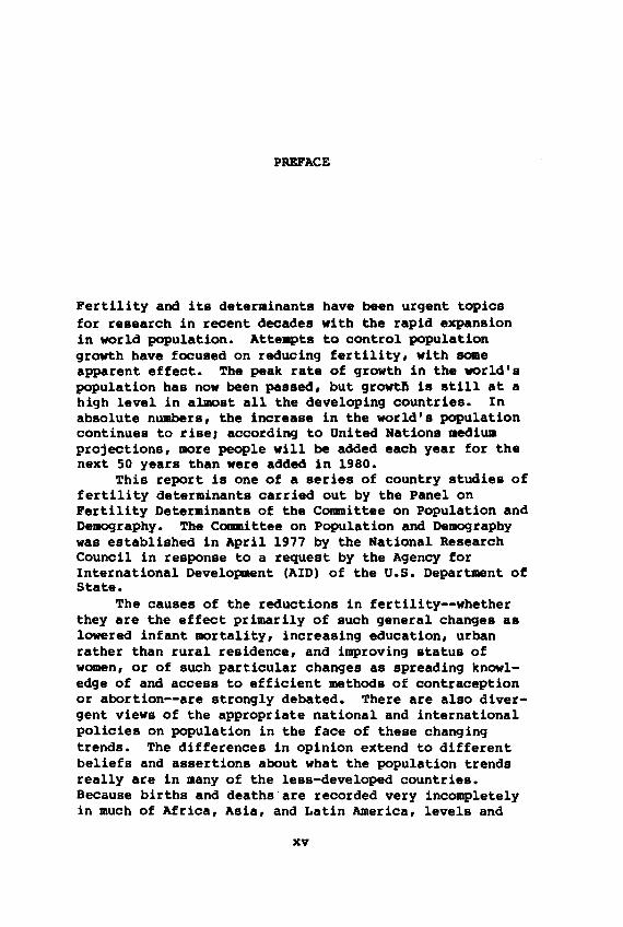
Fertility and its deterainants have been urgent topicsfor research in recent decades with the rapid expansionin world population. Atte~ts to control populationgrowth have focused on reducing fertility, with soaeapparent effect. The peak rate of growth in the world'spopulation has now been passed, but growt~ is still at ahigh level in almost all the developing countries. Inabsolute numbers, the increase in the world's populationcontinues to riseJ according to United Nations mediumprojections, more people will be added each year for thenext 50 years than were added in 1980.

This report is one of a series of country studies offertility determinants carried out by the panel onFertility Determinants of the Committee on Population andDemography. The Committee on Population and Demographywas established in April 1977 by the National ResearchCouncil in response to a request by the Agency forInternational Development (AID) of the U.S. Department ofState.

The causes of the reductions in fertility--whetherthey are the effect primarily of such general changes aslowered infant mortality, increasing education, urbanrather than rural residence, and improving status ofwomen, or of such particular changes as spreading knowl­edge of and access to efficient methods of contraceptionor abortion--are strongly debated. There are also diver­gent views of the appropriate national and internationalpolicies on population in the face of these changingtrends. The differences in opinion extend to differentbeliefs and assertions about what the population trendsreally are in many of the less-developed countries.Because births and deaths'are recorded very incompletelyin much of Africa, Asia, and Latin America, levels and

xv

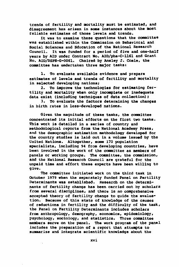
trends of fertility and mortality must be estimated, anddisagreement has arisen in some instances about the MOstreliable estimates of those levels and trends.

It was to examine these questions that the committeewas established within the commission on Behavioral andSocial Sciences and Education of the National ResearchCouncil. It was funded for a period of five and one-halfyears by AID under Contract No. AID/pha-C-ll61 and GrantNo. AID/DSPB-G-0061. Chaired by Ansley J. Coale, thecommittee has Uftdertaken three major tasksl

1. To evaluate available evidence and prepareestimates of levels and trends of fertility and mortalityin selected developing nations,

2. To improve the technologies for estimating fer­tility and mortality when only incomplete or inadequatedata exist (including technique. of data collection) ,

3. To evaluate the factors determining the changesin birth rates in less-developed nations.

Given the magnitude of these tasks, the committeeconcentrated its initial efforts on the first two tasks.This work is detailed in a series of country andmethodological reports from the National Academy Press,and the demographic estimation methodology developed forthe country studies is laid out in a volume issued by theUnited Nations. Altogether, some 170 populationspecialists, including 94 from developing countries, havebeen involved in the work of the committee as members ofpanels or working groups. The committee, the commission,and the National Research Council are grateful for theunpaid time and effort these experts have been willing togive.

The committee initiated work on the third task inOCtober 1979 when the separately funded Panel on FertilityDeterminants was established. Research on the determi­nants of fertility change has been carried out by scholarsfrom several disciplines, and there is no comprehensiveaccepted theory of fertility change to guide the evalua­tion. Because of this state of knowledge of the causesof reductions in fertility and the difficulty of the task,the Panel on Fertility Determinants includes scholarsfrom anthropology, demography, economics, epidemiology,psychology, sociology, and statistics. Three committeemembers serve on the panel. The work program of the panelincludes the preparation of a report that atte~ts tosummarize and integrate scientific knowledge about the

xvi

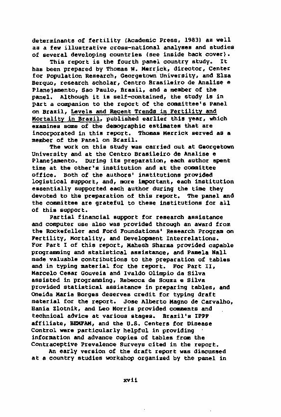
determinants of fertility (Academic Press, 1983) as wellas a few illustrative cross-national analyses and studiesof several developing countries (see inside back cover).

This report is the fourth panel country study. Ithas been prepared by Thomas w. Merr~ck, director, Centerfor popUlation Research, Georgetown University, and ElzaBerquo, research scholar, Centro Brasileiro de Analise ePlanejamento, Sao Paulo, Brazil, and a member of thepanel. Although it is self-contained, the study is inpart a companion to the report of the committee's panelon Brazil, Levels and Recent Trends in Fertility andMortality in Brazil, pUblished earlier this year, whichexamines some of the demographic estimates that areincorporated in this report. Thomas Merrick served as amember of the Panel on Brazil.

The work on this stUdy was carried out at GeorgetownUniversity and at the Centro Brasileiro de Analise ePlanejamento. During its preparation, each author spenttime at the other's institution and at the committeeoffice. Both of the authors' institutions providedlogistical support, and, more important, each institutionessentially supported each author during the time theydevoted to the preparation of this report. The panel andthe committee are grateful to these institutions for allof this support.

Partial financial support for research assistanceand computer use also was provided through an award fromthe Rockefeller and Ford Foundations' Research Program onFertility, Mortality, and Development Interrelations.For Part I of this report, Mahesh Sharma provided capableprogramming and statistical assistance, and Pamela Hallmade valuable contributions to the preparation of tablesand in typing material for the report. For Part II,Marcelo Cesar Gouveia and Ivaldo Olimpio da Silvaassisted in programming, Rebecca de Souza e Silvaprovided statistical assistance in preparing tables, andoneida Maria Borges deserves credit for typing draftmaterial for the report. Jose Alberto Magno de Carvalho,Bania Zlotnik, and Leo Morris provided comments andtechnical advice at various stages. Brazil's IPPFaffiliate, BEMFAM, and the U.S. Centers for DiseaseControl were particularly helpful in providinginformation and advance copies of tables from theContraceptive Prevalence Surveys cited in the report.

An early version of the draft report was discussedat a country studies workshop organized by the panel in

xvii

January 1982 with financial assistance from theRockefeller Foundation. Finally, panel and committeereviewers provided advice and suggestions.

Several members of the panel and committee staffassisted in the preparation of this report. On theproduction side appreciation is expressed to ElaineMcGarraugh of the panel staff for handling the productionediting details, to Solveig Padilla and Irene Martinezfor helping type the text and tables, and to Rona Brierefor editing t~ report.

w. PARKER MAULDIN, ChairPanel on Fertility Determinants

xviii

SUMMARY

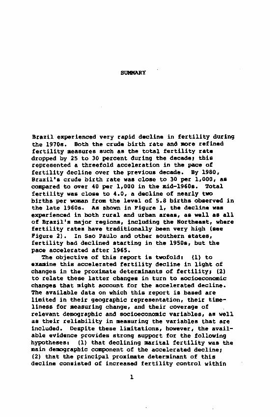
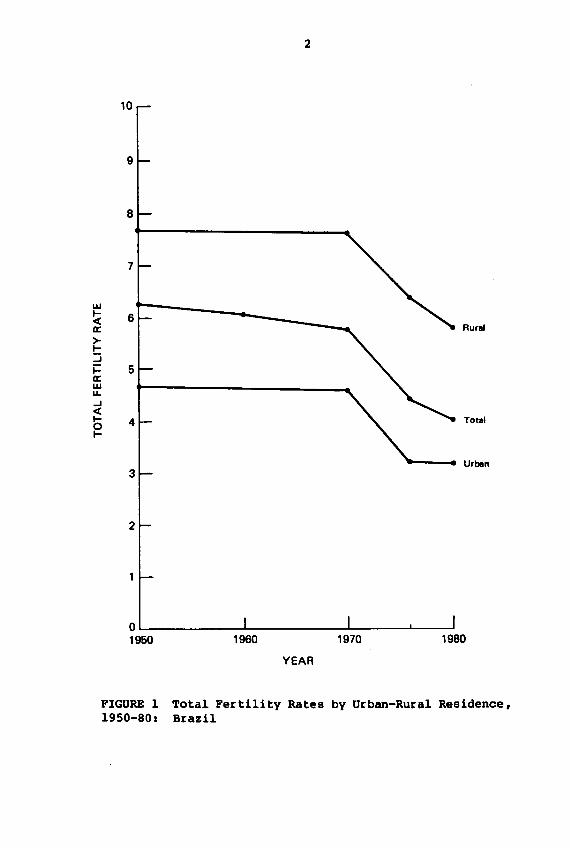
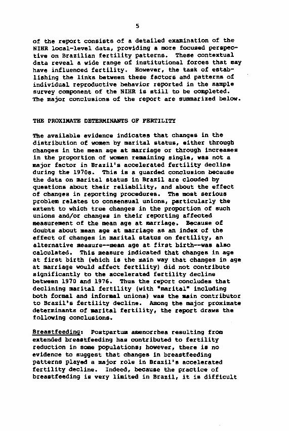
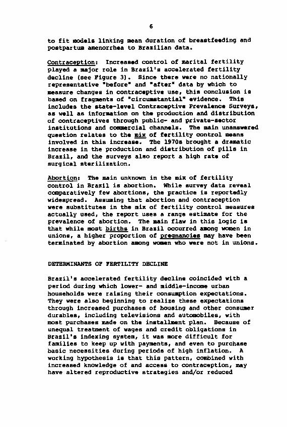
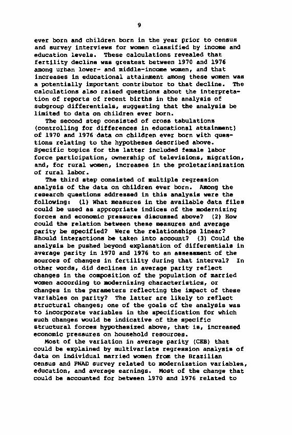
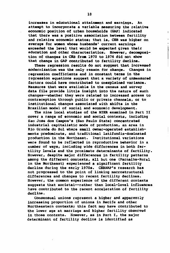
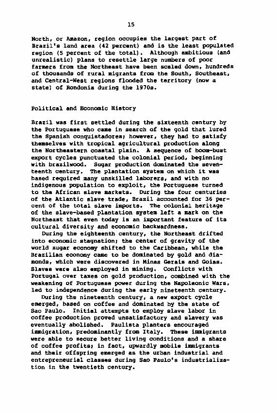
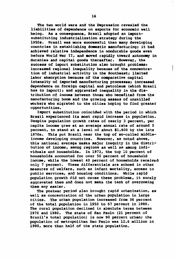
Brazil experienced very rapid decline in fertility duringthe 1970s. Both the crude birth rate and more refinedfertility measures such as the total fertility rat.dropped by 25 to 30 percent during the decade, thisrepresented a threefold acceleration in the pace offertility decline over the previous decade. By 1980,Brazills crude birth rate was close to 30 per 1,000, ascompared to over 40 per 1,000 in the mid-1960s. Totalfertility was close to 4.0, a decline of nearly twobirths per woman from the level of 5.8 births observed inthe late 1960s. As shown in Figure 1, the decline wasexperienced in both rural and urban areas, as well as allof Brazills major regions, including the Northeast, wherefertility rates have traditionally been very high (seeFigure 2). In Sao Paulo and other southern states,fertility had declined starting in the 1950s, but thepace accelerated after 1965.

The objective of this report is twofold: (1) toexamine this accelerated fertility decline in light ofchanges in the proximate determinants of fertility, (2)to relate these latter changes in turn to socioeconomicchanges that might account for the accelerated decline.The available data on which this report is based arelimited in their geographic representation, their time­liness for measuring change, and their coverage ofrelevant demographic and socioeconomic variables, as wellas their reliability in measuring the variables that areincluded. Despite these limitations, however, the avail­able evidence provides strong support for the followinghypotheses: (1) that declining marital fertility was themain demographic component of the accelerated decline,(2) that the principal proximate determinant of thisdecline consisted of increased fertility control within

1

2

10

9

8

7

wI- 6«II: Rurel

>!::..J

i= 5II:WLL..J«I- 4 Totel0I-

Urben3

2

198019701960

O'--- ---'- .l..-__----J'---_---'

1950

YEAR

FIGURE 1 Total Fertility Rates by Urban-Rural Residence,1950-80: Brazil

3

9

8

10

7

wl- e«a: North-

~ Eastern

...JStlI...

~ 5a:wlL. Milllll...J Gerail'« 4 EtplrltoI-

~SIInto

SouthernStlI'"

3 SIlo Paulo

Rio deJaneiro

2

198019701960

0'-- -'- --'- --'-_----'

1950

YEAR

FIGURE 2 Total Fertility Rates by Region, 1950-80:Brazil

4

marriage (contraception, sterilization, and abortion) ,though it was not possible to specify precisely what the·mix· of these determinants was or how it may havechanged, (3) that the decline in marital fertility can beattributed mainly to the spread of fertility control tolower-income regions and groups that had not participatedin previous fertility declines, and (4) that these groupsexperienced socioeconoaic changes (for exaaple, increasededucational attai~nt, increased ownership of such con­sumer durable goods as televisions, and increased femalelabor force participation) that were conducive to -.allerfamily nor...

This report is baaed mainly on three sources of infor­mation. The first consists·of national-level data col­lected by the Brazilian census bureau (Pundacao InstitutoBrasileiro de Geografia e Bstatistica--FIBGE), includingthe 1970 population census and a 1976 national s.-plesurvey (Pesquisa Nacional por ~stra de Domicilios-­PNAD). Both included retrospective questions on fer­tility as well as on socioeconoaic characteristics. Thesecond source is the state-level Contraceptive PrevalenceSurveys (CPS) conducted during the late 1970s by BrazillsInternational Planned Parenthood affiliate, BBMFAM (Soc­iedade Civil de Bem-Bstar Familiar), with the assistanceof the u.S. Center for Disease Control. Finally, a sourceat the local level is the CBBRAP National Investigationof Buaan Reproduction (NIBR), which consists of in-depthcontextual studies of nine caaaunities representing dif­ferent types of socioeconoaic structure in Brazil, aswell as -.all s.-ple surveys of the reproductive lifehistories of women in those settings. When possible,other sources are used to provide supplemental informa­tion.

The report is presented in two parts. The first usesthe national- and state-level data to examine severalhypotheses about how socioeconoaic changes may haveinfluenced the reproductive behavior of different groupsin Brazil during the early 1970s. Tabular and mUltipleregression analyses of these data provide strong supportfor the argument that increased educational attai~nt ofwomen contributed to the modernization of reproductivebehavior, though the data do not provide enough informa­tion to specify precisely how this occurred. Nor do theypermit as full a testing as one would desire of hypothesesabout the way in which institutional forces and structuralfactors arising from class differences and economic pres­sures influenced reproductive patterns. The second part

5

of the report consists of a detailed examination of theNIHR local-level data, providing a more focused perspec­tive on Brazilian fertility patterns. These contextualdata reveal a wide range of institutional forces that mayhave influenced fertility. However, the task of estab­lishing the links between these factors and patterns ofindividual reproductive behavior reported in the samplesurvey component of the NIHR is still to be completed.The major conclusions of the report are summarized below.

THE PROXIMATE DETERMINANTS OF FERTILITY

The available evidence indicates that changes in thedistribution of women by marital status, either throughchanges in the mean age at marriage or through increasesin the proportion of women remaining single, was not amajor factor in Brazil's accelerated fertility declineduring the 1970s. This is a guarded conclusion becausethe data on marital status in Brazil are clouded byquestions about their reliability, and about the effectof changes in reporting procedures. The JIOst seriousproblem relates to consensual unions, particularly theextent to which true changes in the proportion of suchunions and/or changes in their reporting affectedmeasurement of the mean age at marriage. Because ofdoubts about mean age at marriage as an index of theeffect of changes in marital status on fertility, analternative measure--mean age at first birth--was alsocalculated. This measure indicated that changes in ageat first birth (which is the main way that changes in ageat marriage would affect fertility) did not contributesignificantly to the accelerated fertility declinebetween 1970 and 1976. Thus the report concludes thatdeclining marital fertility (with -marital- includingboth formal and informal unions) was the main contributorto Brazil's fertility decline. Among the major proximatedeterminants of marital fertility, the report draws thefollowing conclusions.

Breastfeeding: Postpartum amenorrhea resulting fromextended breastfeeding has contributed to fertilityreduction in some populations, however, there is noevidence to suggest that changes in breastfeedingpatterns played a major role in Brazil's acceleratedfertility decline. Indeed, because the practice ofbreastfeeding is very limited in Brazil, it is difficult

6

to fit models linking mean duration of breastfeeding andpostpartum amenorrhea to Brazilian data.

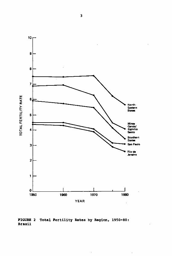
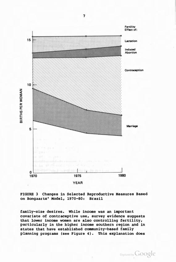
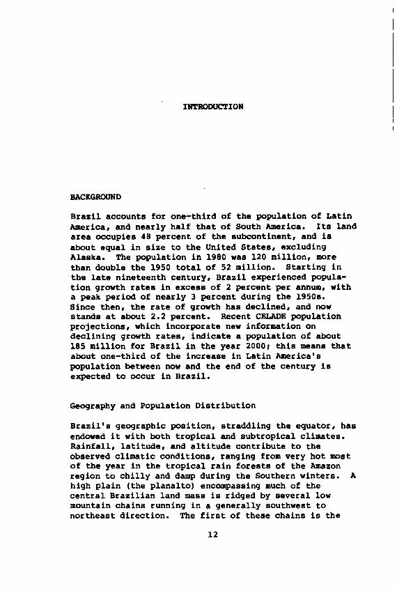
Contraceptions Increased control of marital fertilityplayed a major role in Brazil's accelerated fertilitydecline (see Figure 3). Since there were no nationallyrepresentative -before- and -after- data by which tomeasure changes in contraceptive use, this conclusion isbased on fragments of -circuastantial- evidence. Thisincludes the .tate-level Contraceptive Prevalence Surveys,as well as information on the production and distributionof contraceptives through public- and private-sectorinstitutions and commercial channels. The main unansweredquestion relates to the ~ of fertility control meansinvolved in this increase. The 1970s brought a draaaticincrease in the production and distribution of pills inBrazil, and the surveys also report a high rate ofsurgical sterilization.

Abortions The main unknown in the mix of fertilitycontrol in Brazil is abortion. While survey data revealcomparatively few abortions, the practice is reportedlywidespread. Assuming that abortion and contraceptionwere substitutes in the mix of fertility control measuresactually used, the report uses a range estimate for theprevalence of abortion. The main flaw in this logic isthat while most births in Brazil occurred among women inunions, a higher proportion of pregnancies may have beenterminated by abortion among women who were not in unions.

DETEBMINANTS OF FERTILITY DECLINE

Brazil's accelerated fertility decline coincided with aperiod during which lower- and middle-income urbanhouseholds were raising their consumption expectations.They were also beginning to realize these expectationsthrough increased purchases of housing and other consumerdurables, including televisions and automobiles, withmost purchases made on the installment plan. Because ofunequal treatment of wages and credit obligations inBrazil's indexing system, it was more difficult forfamilies to keep up with paYments, and even to purchasebasic necessities during periods of high inflation. Aworking hypothesis is that this pattern, combined withincreased knowledge of and access to contraception, mayhave altered reproductive strategies and/or reduced

7

FertilitYEffect of:

z<{:!:o:ita::wQ..(J)

:I:~a::iii

15

10

5

Lactation

InducedAbortion

Contraception

Marriage

19801975

YEAR

OL...- ...l--_L- --'-'

1970

FIGURE 3 Changes in Selected Reproductive Measures Basedon Bongaarts' Model, 1970-80: Brazil

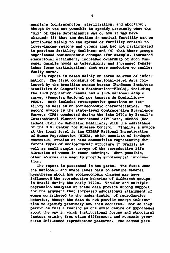
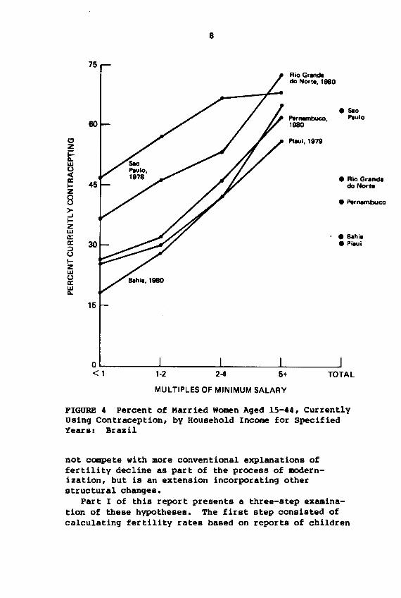
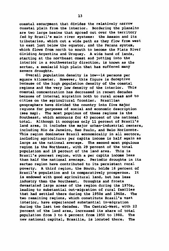
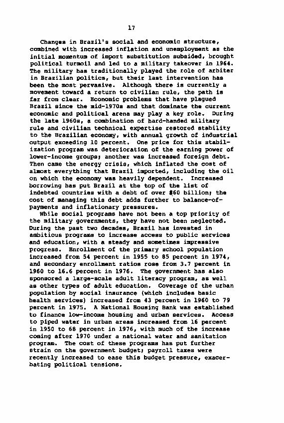
family-size desires. While income was an importantcovariate of contraceptive use, survey evidence suggeststhat lower income women are also controlling fertility,particularly in the higher income southern region and instates that have established community-based familyplanning programs (see Figure 4). This explanation does

D,qll,ZE j byCoogIe

8

75Rio Grendedo Norte, 1980

• saoPernembuco, "-ulo1980

C) P....l.1979Z

t"w(,Jc(

• Rio Grandea:~ do NoruZ

8 • "-rnambuco>-..J~ZWII: • Bah18II: • Pi8Ui::J(,J

~zw(,JII:W~

15

TOTAL5+2-41-2

O'------'-- L- ----lL...- ---J

<1

MULTIPLES OF MINIMUM SALARY

FIGURE 4 Percent of Married Women Aged 15-44, CurrentlyUsing Contraception, by Household Income for SpecifiedYears: Brazil

not compete with more conventional explanations offertility decline as part of the process of modern­ization, but is an extension incorporating otherstructural changes.

Part I of this report presents a three-step examina­tion of these hypotheses. The first step consisted ofcalculating fertility rates based on reports of children

9

ever born and children born in the year prior to censusand survey interviews for women classified by income andeducation levels. These calculations revealed thatfertility decline was greatest between 1970 and 1976among urban lower- and middle-income women, and thatincreases in educational attainment among these women wasa potentially important contributor to.that decline. Thecalculations also raised questions about the interpreta­tion of reports of recent births in the analysis ofsubgroup differentials, suggesting that the analysis belimited to data on children ever born.

The second step consisted of cross tabulations(controlling for differences in educational attainment)of 1970 and 1976 data on children ever born with ques­tions relating to the hypotheses described above.Specific topics for the latter included female laborforce participation, ownership of televisions, migration,and, for rural women, increases in the proletarianizationof rural labor.

The third step consisted of multiple regressionanalysis of the data on children ever born. Among theresearch questions addressed in this analysis were thefollowing I (1) What measures in the available data filescould be used as appropriate indices of the modernizingforces and economic pressures discussed above? (2) Howcould the relation between these measures and averageparity be specified? Were the relationships linear?Should interactions be taken into account? (3) Could theanalysis be pushed beyond explanation of differentials inaverage parity in 1970 and 1976 to an assessment of thesources of changes in fertility during that interval? Inother words, did declines in average parity reflectchanges in the composition of the population of marriedwomen according to modernizing characteristics, orchanges in the parameters reflecting the impact of thesevariables on parity? The latter are likely to reflectstructural changes, one of the goals of the analysis wasto incorporate variables in the specification for whichsuch changes would be indicative of the specificstructural forces hypothesized above, th~ is, increasedeconomic pressures on household resources.

Most of the variation in average parity (CEB) thatcould be explained by multivariate regression analysis ofdata on individual married women from the Braziliancensus and PNAD survey related to modernization variables,education, and average earnings. Most of the change thatcould be accounted for between 1970 and 1976 related to

10

increaaes in educational attai~nt and earnings. Anattempt to incorporate a variable measuring the relativeeconomic position of urban households (GAP) indicatedthat there was a positive association between fertilityand relative econoaic status, that is, CEB was higher onaverage for women whose husbands' current earningsexceeded the level that would be expected given theireducation and other characteristics. However, decomposi­tion of changes in CBB froa 1970 to 1976 did not showthat change in GAP contributed to fertility decline.

These regression results do not suggest that increaaedmodernization was the only reason for change. Changes inregression coefficients and in constant terms in theregression equations suggest that a variety of unmeasuredfactors could have contributed to unexplained variance.Measures that were available in the census and surveydata file provide little insight into the nature of suchchanges--whether they were related to increased access tocontraception through public or private channels, or toinstitutional changes associated with shifts in theBrazilian model of social and economic development.

The nine local studies of the NIBR examined in Part IIcover a range of economic and social contexts, includingSao Jose dos Campos's (Sao Paulo State) concentratedindustrial capitalistic mode of production, an area inRio Grande do Sul where small owner-operated establish­ments predominate, and traditional latifundia-dominatedproduction in the Northeast. Institutional variationswere found to be reflected in reproductive behavior in anumber of ways, inclUding wide differences in both fer­tility levels and the proximate determinants of fertility.However, despite major differences in fertility patternsamong the different contexts, all but one (Parnaiba-Ruralin the Northeast) experienced a significant fertilitydecline during the early 1970s. CEBRAP's research hasnot progressed to the point of linking macrostructuraldifferences and changes to recent fertility declines.However, the cammon experience of the different contextssuggests that societal--rather than ~ocal-level influenceshave contributed to the recent acceleration of fertilitydecline.

Consensual unions represent a higher and apparentlyincreasing proportion of unions in Recife and otherNortheastern contexts, this fact may have contributed tothe lower age at marriage and higher fertility observedin those contexts. However, as in Part I, the majordeterminant of fertility decline is identified as

11

declining marital fertility. Again as in Part I, themain proximate determinant of this decline in maritalfertility was found to be increased use of contraception,particularly the more effective methods. This can inturn be related at the local level to shifts in familyincome: as in Part I, it is concluded that there is apositive association between higher family income anddecreased family size.

INTRODUCTION

BACKGROUND

Brazil accounts for one-third of the population of LatinAmerica, and nearly half that of South America. Its landarea occupies 48 percent of the subcontinent, and isabout equal in size to the United States, excludingAlaska. The population in 1980 was 120 million, morethan double the 1950 total of 52 million. Starting inthe late nineteenth century, Brazil experienced popula­tion growth rates in excess of 2 percent per annum, witha peak period of nearly 3 percent during the 1950s.Since then, the rate of growth has declined, and nowstands at about 2.2 percent. Recent CELADE populationprojections, which incorporate new information ondeclining growth rates, indicate a population of about185 million for Brazil in the year 2000, this means thatabout one-third of the increase in Latin America'spopulation between now and the end of the century isexpected to occur in Brazil.

Geography and Population Distribution

Brazil's geographic position, straddling the equator, hasendowed it with both tropical and subtropical climates.Rainfall, latitude, and altitude contribute to theobserved climatic conditions, ranging from very hot mostof the year in the tropical rain forests of the Amazonregion to chilly and damp during the SOuthern winters. Ahigh plain (the planalto) encompassing much of thecentral Brazilian land mass is ridged by several lowmountain chains running in a generally southwest tonortheast direction. The first of these chains is the

12

13

coastal escarpment that. divides the relatively narrowcoastal plain from the interior. Bordering the planaltoare two large basins that spread out over the territoryfed by Brazil's main river systems: the Amazon and itstributaries, which cut a wide path as they flow from westto east just below the equator, and the Parana system,which flows from north to south to become the Plata Riverdividing Argentina and Uruguay. A wide band of lands,starting at the northeast coast and jutting into theinterior in a southwesterly direction, is known as thesertao, a semiarid high plain that has suffered manysevere droughts.

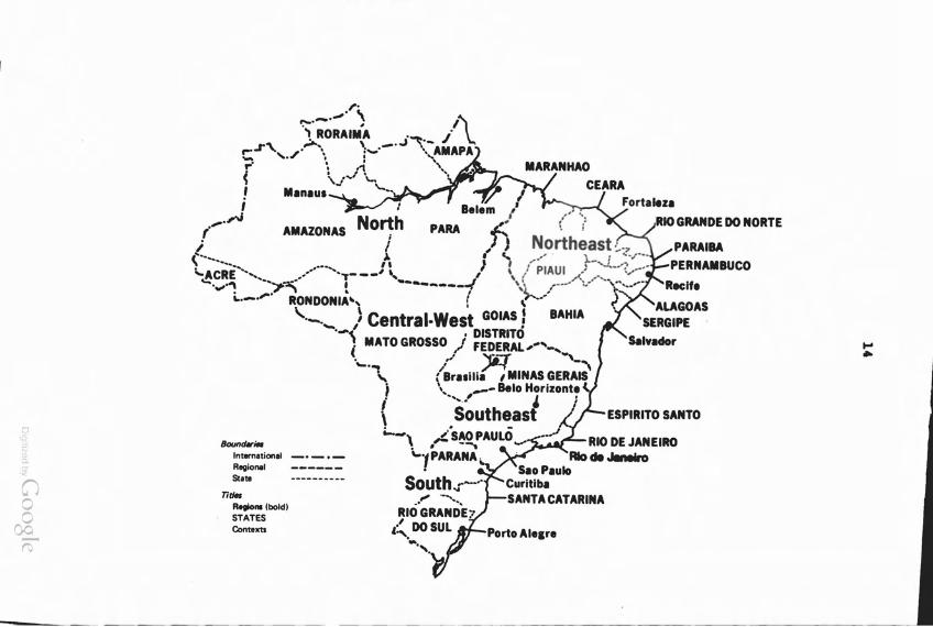
Overall population density is low--14 persons persquare kilometer. However, this figure is deceptivebecause of the high population density of the coastalregions and the very low density of the interior. Thiscoastal concentration has decreased in recent decadesbecause of internal migration both to rural areas and tocities on the agricultural frontier. Braziliangeographers have divided the country into five majorregions for purposes of social and economic description(see map). The most populous of these regions is theSoutheast, which accounts for 43 percent of the nationaltotal. Although it occupies only 11 percent of Brazil'sland area, it includes the major urban-industrial centers,including Rio de Janeiro, Sao Paulo, and Belo Horizonte.This region dominates Brazil economically in all sectors,including agriculture, per capita income is half again aslarge as the national average. The second most populousregion is the Northeast, with 29 percent of the totalpopulation and 18 percent of the land area. This isBrazil's poorest region, with a per capita income lessthan half the national average. Periodic droughts in itssertao region have contributed to its persistent ruralpoverty. A third region, the South, holds 16 percent ofBrazil's population and is comparatively prosperous. Itis endowed with good agricultural land, but has lessindustry than the Southeast. Droughts and frostsdevastated large areas of the region during the 1970s,leading to substantial out-migration of rural familiesthat had settled there during the 1950s and 1960s. Thetwo remaining regions, which constitute Brazil's vastinterior, have experienced substantial in-migrationduring the last two decades. The Central-West, with 22percent of the land area, increased its share of totalpopulation from 3 to 6 percent from 1950 to 1980. Thenew national capital, Brasilia, is located there. The

....~

PARAIBA

PERNAMBUCO

Recife

ESPIRITO SANTO

MARANHAO

CEARA,Fort.lez.

RIO DE JANEIRO• • .......-0

SuP.uloCuritlb.SANTA CATARINA

AMAZONAS

n,.Regions (bold)STATESContexts

1Joumkr_InternltionalRogionolState

,."",' ..

.....-. \ '\'" RORAIM'A '. i..... ,... \ _ . ..J",-,.."" I'" :...... '" AMAPA..... ,...... I •

r- ~ ~

( \J"J \ .I M.n.u.-.... ..........,; -

_.;oJ

";( ............_,'".!CRE ...... .....__."\ ~~ · --------r V ,-

~.-..... RONDONIA', i .)-.....\. \ , ...__ I Central-West GOlAS1 BAHIA

._{ , DISTRITO( MATO GROSSO) FEDERAL,.....- ...

...... ..~. "JL{ ""'-""\... \ Br..m. , MINAS GERAIS

; '. _- &elo Horizontei -.......' ~:

\ Southeasti-._, ,,"SAO PAULO.' -~'-'1 PARANA.

South.r-··,.. -...~. ...

RIOGRANDE7

l~. DOSUL-.,.

9~

,

~

CJo

C'2-rv

15

North, or Amazon, region occupies the largest part ofBrazil's land area (42 percent) and is the least populatedregion (5 percent of the total). Although ambitious (andunrealistic) plans to resettle large numbers of poorfarmers from the Northeast have been scaled down, hundreds

. of thousands of rural migrants from the South, Southeast,and Central-West regions flooded the territory (now astate) of Rondonia during the 1970s.

Political and Economic History

Brazil was first settled during the sixteenth century bythe Portuguese who came in search of the gold that luredthe Spanish conquistadores, however, they had to satisfythemselves with tropical agricultural production alongthe Northeastern coastal plain. A sequence of ~bustexport cycles punctuated the colonial period, beginningwith brazilwood. Sugar production dominated the seven­teenth century. The plantation system on which it wasbased required many unskilled laborers, and with noindigenous population to exploit, the Portuguese turnedto the African slave markets. During the four centuriesof the Atlantic slave trade, Brazil accounted for 36 per­cent of the total slave imports. The colonial heritageof the slave-based plantation system left a mark on theNortheast that even today is an important feature of itscultural diversity and economic backwardness.

During the eighteenth century, the Northeast driftedinto economic stagnation, the center of gravity of theworld sugar economy shifted to the Caribbean, while theBrazilian economy came to be dominated by gold and dia­monds, which were discovered in Minas Gerais and Goias.Slaves were also employed in mining. Conflicts withPortugal over taxes on gold production, combined with theweakening of Portuguese power during the Napoleonic Wars,led to independence during the early nineteenth century.

During the nineteenth century, a new export cycleemerged, based on coffee and dominated by the state ofSao Paulo. Initial attempts to employ slave labor incoffee production proved unsatisfactory and slavery waseventually abolished. Paulista planters encouragedimmigration, predominantly from Italy. These immigrantswere able to secure better living conditions and a shareof coffee profits, in fact, upwardly mobile immigrantsand their offspring emerged as the urban industrial andentrepreneurial classes during Sao Paulo's industrializa­tion in the twentieth century.

16

The two world wars and the Depression revealed theliabilities of dependence on exports for economic wellbeing. As a consequence, Brazil adopted an import­substituting industrialization strategy during the1950s. Brazil was more successful than .any developingcountries in establishing da.estic aanufacturing, it hadachieved relative independence in nondurable goods evenbefore World War II, and .aved rapidly toward auto~ indurables and capital goods thereafter. However, thesuccess of import sUbstitution also brought probleasaincreased regional inequality because of the concentra­tion of industrial activity in the SOutheast, limitedlabor absorption because of the comparative capitalintensity of imported manufacturing processes, increaseddependence on foreign capital and petrolea (which Brazilhas to import), and aggravated inequality in the dis­tribution of income between those who benefited from themanufacturing boom and the growing masses of unskilledworkers who migrated to the cities hoping to find greateropportunities.

Import substitution coincided with the period in whichBrazil experienced its most rapid increase in population.Despite population growth rates of nearly 3 percent, percapita income grew at an average annual rate of around 5percent, to stand at a level of about $1,600 by the late1970s. This put Brazil near the top of so-called middle­income developing countries. However, as noted above,this national average masks major inequity in the distri­bution of income, among regions as well as among indi­viduals and households. In 1972, the top 10 percent ofhouseholds accounted for over 50 percent of householdincome, while the lowest 40 percent of households receivedonly 7 percent. These differentials are echoed in othermeasures of welfare, such as infant mortality, access topublic services, and housing conditions. While rapidpopulation growth did not cause these problems, it surelyaggravated them and does not make the task of overcomingthem any easier.

The postwar period also brought rapid urbanization, aswell as concentration of the urban population in largecities. The urban population increased from 36 percentof the total population in 1950 to 67 percent in 1980.The rural population declined in absolute terms between1970 and 1980. The state of Sao Paulo (21 percent ofBrazil's total population) is now 90 percent urban, thepopulation of metropolitan Sao Paulo was 12.6 million in1980, more than half of the state population.

17

Changes in Brazil's social and economic structure,combined with increased inflation and unemployment as theinitial momentum of import substitution subsided, broughtpolitical turmoil and led to a military takeover in 1964.The military has traditionally played the role of arbiterin Brazilian politics, but their last intervention hasbeen the most pervasive. Although there is currently amovement toward a return to civilian rule, the path isfar from clear. Economic problems that have plaguedBrazil since the mid-1970s and that dominate the currenteconomic and political arena may playa key role. Duringthe late 1960s, a combination of hard-handed militaryrule and civilian technical expertise restored stabilityto the Brazilian economy, with annual growth of industrialoutput exceeding 10 percent. One price for this stabil­ization program was deterioration of the earning power oflower-income groups, another was increased foreign debt.Then came the energy crisis, which inflated the cost ofalmost everything that Brazil imported, including the oilon which the economy was heavily dependent. Increasedborrowing has put Brazil at the top of the list ofindebted countries with a debt of over $60 billion, thecost of managing this debt adds further to balance-of­payments and inflationary pressures.

While social programs have not been a top priority ofthe military governments, they have not been neglected.During the past two decades, Brazil has invested inambitious programs to increase access to pUblic servicesand education, with a steady and sometimes impressiveprogress. Enrollment of the primary school populationincreased from 54 percent in 1955 to 85 percent in 1974,and secondary enrollment ratios rose from 3.7 percent in1960 to 16.6 percent in 1976. The government has alsosponsored a large-scale adult literacy program, as wellas other types of adult education. Coverage of the urbanpopulation by social insurance (which includes basichealth services) increased from 43 percent in 1960 to 79percent in 1975. A National Housing Bank was establishedto finance low-income housing and urban services. Accessto piPed water in urban areas increased from 16 percentin 1950 to 68 percent in 1976, with much of the increasecoming after 1970 under a national water and sanitationprogram. The cost of these programs has put furtherstrain on the government budget, payroll taxes wererecently increased to ease this budget pressure, exacer­bating political tensions.

18

RECENT DEMOGRAPHIC TRENDS

Population Trends

At the beginning of the nineteenth century, the Brazilianpopulation numbered about three and one-third million,two million were either slaves or former slaves who hadbeen manumitted. By 1900, the population was nearly 18million, with recent European immigrants representing anincreasingly important group. Cultural and ethnic diver­sity, an important dimension of the Brazilian socialstructure, has proved difficult to measure in standardstatistics. Complex patterns of interracial marriage andself-declaration of race in four categories (white, black,yellow, and mixed) in Brazilian censuses led to suchskepticism about the validity of the data that the ques­tion was abandoned in 1970. Though the question wasreintroduced in 1980, there is a major void in data onthe ethnic aspects of Brazil's recent demographic history.

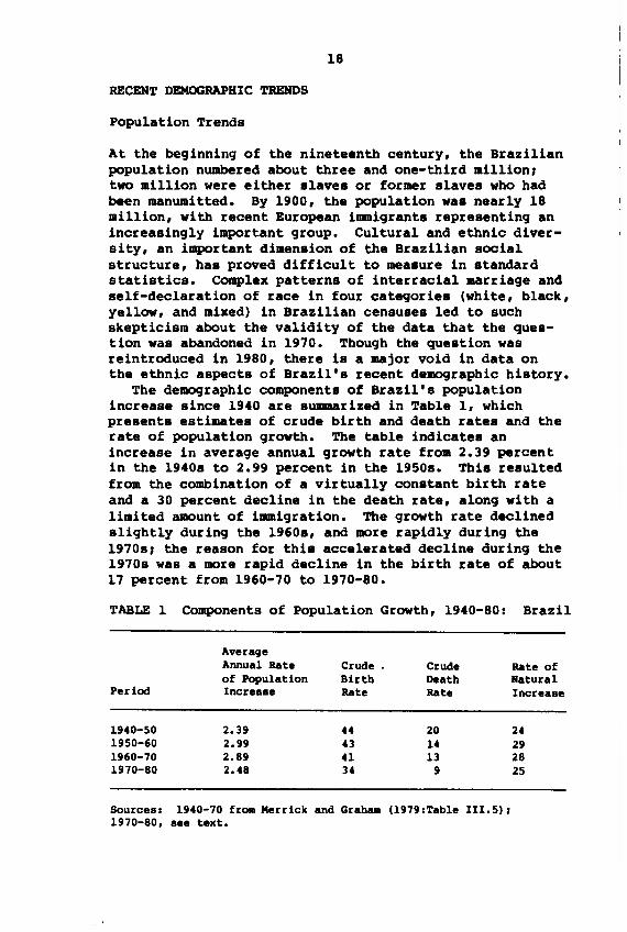
The demographic components of Brazil's populationincrease since 1940 are summarized in Table 1, whichpresents estimates of crude birth and death rates and therate of population growth. The table indicates anincrease in average annual growth rate from 2.39 percentin the 1940s to 2.99 percent in the 1950s. This resultedfrom the combination of a virtually constant birth rateand a 30 percent decline in the death rate, along with alimited amount of immigration. The growth rate declinedslightly during the 1960s, and more rapidly during the1970s, the reason for this accelerated decline during the1970s was a more rapid decline in the birth rate of about17 percent from 1960-70 to 1970-80.

TABLE 1 Components of Population Growth, 1940-80: Brazil

Averll9eAnnual Rate Crude. Crude Rate ofof Population Birth Death Natural

Period Increase Rate Rate Increase

1940-50 2.39 44 20 241950-60 2.99 43 14 291960-70 2.89 41 13 281970-80 2.48 34 9 25

Sources: 1940-70 from Merrick and Graham (1979:Tab1e III.5)J1970-80, see text.

19

As with other features of Brazilian economic and socialhistory, these national-level data mask important regionaldifferentials. The pace of change in both mortality andfertility has varied substantially between the moreurbanized Southeast and the rest of Brazil, most strik­ingly in comparison with the Northeast. Both the leveland timing of such regional differentials can be clari­fied by more refined measures of fertility and mortality,the total fertility rate, and the expectation of life atbirth.

The main sources of nationa1- and regional-level dataon fertility and mortality rates in Brazil are thedecennial censuses and the national sample survey program(Pesquisa Naciona1 por Amostra de Domicilios--PNAD).Though Brazil started to collect vital statistics at thenational level in 1914, coverage is still not adequate topermit assessment of national levels and trends (Altmannand Ferreira, 1919). However, starting with the 1940census, Brazil began reporting the number of childrenever born and the number of children surviving by age ofmother. A question on the number of births in the yearprior to the interview was added in the 1910 census, andwas continued in sample surveys taken in 1912 through1915. In 1916, this question was modified to specify thedate of the last live birth, a procedure that was alsoused in the 1980 census (see Leite, 1981:Tab1e 1).Brazilian demographers, and more recently the Panel onBrazil of the Committee on Population and Demography,National Academy of Sciences, have derived estimates offertility and mortality from these data using indirectestimating techniques. The panel based its estimates onthe census data for 1940-10 and the PNAD survey datathereafter. As the present report was being written,preliminary tabulations of the 1980 census became avail­able. These tabulations are based on an approximatelyone-percent sample of questionnaires processed in advanceof the definitive tabulations, which are scheduled toappear on a state-by-state basis. Where possible, esti­mates based on these preliminary results are introduced.The Panel's fertility and mortality estiwates for 1950-16are reported in Tables 2 and 3, and detailed discussionof data sources and measurement techniques is presentedin their report (National Academy of Sciences, 1919).

20

National and Regional Trends in the Total Fertility Rate

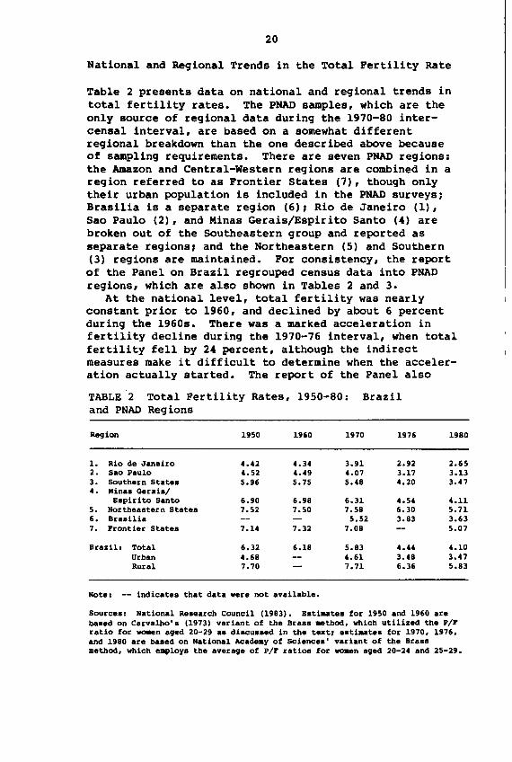
Table 2 presents data on national and regional trends intotal fertility rates. The PNAO samples, which are theonly source of regional data during the 1970-80 inter­censal interval, are based on a somewhat differentregional breakdown than the one described above becauseof sampling requirements. There are seven PNAO regions:the Amazon and Central-Western regions are combined in aregion referred to as Frontier States (7), though onlytheir urban population is included in the PNAD surveysJBrasilia is a separate region (6), Rio de Janeiro (1),Sao Paulo (2), and Minas Gerais/Espirito Santo (4) arebroken out of the Southeastern group and reported asseparate regions, and the Northeastern (5) and Southern(3) regions are maintained. For consistency, the reportof the Panel on Brazil regrouped census data into PNADregions, which are also shown in Tables 2 and 3.

At the national level, total fertility was nearlyconstant prior to 1960, and declined by about 6 percentduring the 1960s. There was a marked acceleration infertility decline during the 1970-76 interval, when totalfertility fell by 24 percent, although the indirectmeasures make it difficult to determine when the acceler­ation actually started. The report of the Panel also

TABLE 2 Total Fertility Rates, 1950-80: Braziland PNAD Regions

RlI9 i on 1950 1960 1970 1976 1980

1- Rio de Janeiro 4.42 4.34 3.91 2.92 2.652. Sao Paulo 4.52 4.49 4.07 3.17 3.133. SOuthern Statea 5.96 5.75 5.48 4.20 3.474. Minas Gerais/

Bapirito Santo 6.90 6.98 6.31 4.54 4.115. Northeastern States 7.52 7.50 7.58 6.30 5.7l6. Brasilia 5.52 3.83 3.637. Frontier States 7.14 7.32 7.08 5.07

Brazil: Total 6.32 6.18 5.83 4.44 4.10Urban 4.68 4.61 3.48 3.47Rural 7.70 7.71 6.36 5.83

Note: -- indicates that data were not available.

Sources: National Research Council (1983). Bstiaates for 1950 and 1960 arebased on Carvalho's (1973) variant of the Brass ..thod, which utilized the P/Fratio for ~n aged 20-29 as diacussed in the text, estiaates for 1970, 1976,and 1980 are based on National Academy of SCiences' variant of the Brassmethod, which employs the average of P/F ratios for wa.en aged 20-24 and 25-29.

21

provides estimates of total fertility based on the own­children method which suggest that total fertility in1969-70 was lower than 5.8. In all likelihood, thedecline in the national total fertility rate acceleratedin the late 1960s.

This national trend once again masks major regionaldifferentials. The transition to lower fertility wasalready well underway in Rio de Janeiro and Sao Pauloduring the 1950s, with total fertility nearly 2 childrenper woman lower than the national average by 1970. Amore gradual decline was underway in the southern statesand in Minas Gerais/Espirito Santo. In contrast, fertil­ity in the Northeast and in the Frontier states was high,possibly increasing, before 1970. Regional differentialsincreased during the 1950-70 period, but declines in theSoutheast were not great enough to have a significantimpact on the national trend. In the rural-urban break­down, there was little change from 1950 to 1970 ineither, this suggests that the limited national declineresulted in large part from the increased weight of theurban population in the total.

The 1970-76 period brought accelerated declines in allregions. In the Southern and Southeastern regions, ratesfell by 22-28 percent, with the greatest decline occurringin region (4) (Minas Gerais/Espirito Santo). While thedecline in the Northeast was less--17 percent--it signaledan important increase in the spread of accelerated fer­tility decline. At the same time, the Northeast-Southeastdifferential increased. Since rates of decline in theSoutheastern states have reached comparatively low levels,continuation of the national trend will depend to a largeextent on the pace at which Northeastern states catch up.

Estimates based on preliminary tabulations of the 1980census indicate that the trend observed for the 1970-76period continued during 1976-80, though at a slower pace.The 1980 total fertility rate for Brazil, 4.11, is 7.7percent less than the 4.44 recorded in 1976 and 29.7percent less than the 1970 rate of 5.83. Total fertilityin the Southern region declined most (17.7 percent)during 1976-80, making this the region with the largestoverall decline (36.7 percent) over the decade. Region(4) (Minas Gerais/Espirito Santo) ranked second in1976-80, with 9.5 percent, and also second for thedecade, with 34.9 percent. It is significant that theNortheast, which ranked last during the 1970-76 interval,was third in 1976-80 with a 9.4 percent decline, sincethis suggests that the spread of fertility decline to the

22

Northeast has continued and even accelerated. For thedecade, this put the Northeast just ahead of Sao Paulo,which had a very small decline (1.3 percent) during1976-80 and ranked last for the decade with 23.1 percent.Both Rio de Janeiro and the Frontier states were within apoint or two of the national average, suggesting thatomission of rural areas of the Frontier from the 1976results probably did not bias the rate reported forBrazil at that date.

A surprising feature of the 1980 results is that theyindicate that fertility decline during the 1976-80 periodwas limited to rural areas, total fertility for urbanareas was practically unchanged over that interval. Thisraises a number of questions, to which the limited datapublished in the preliminary tabulations provide very fewanswers. One of these questions relates to the reliabil­ity of the sample frame on which the 1976 survey wasbased. It may be that the -Brazil- sampled in the 1976survey underrepresented groups that experienced slowerfertility decline, leading to an overstatement of thedecline from 1970 to 1976 and an understatement of thedecline from 1976 to 1980. If this was not the case,there is an even more interesting question of why urbanfertility decline accelerated (to 24.5 percent) duringthe early 1970s and dropped to zero at the end of thedecade. Was there a baby -boomlet- during the late1970s? Clearly, we need a thoroughgoing assessment ofthe representativeness of the PNAD surveys, as well as acomparison of the advanced tabulations against thedefinitive 1980 census results. Although both of thesetasks run well beyond the scope of this report, they havemajor implications for the present analysis of trends inthe 1970s, which relies heavily on data from the 1976survey.

Expectation of Life at Birth

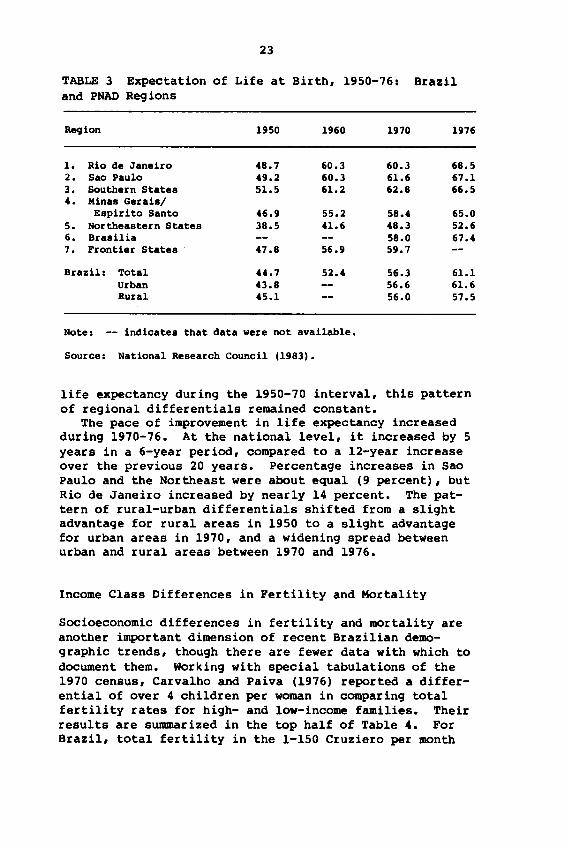
Table 3 presents estimates of national and regionaltrends in the expectation of life at birth. In contrastwith total fertility, there is a substantial increase (26percent) in life expectancy at the national level. Thereare also important regional differentials, with the North­east lagging behind the rest of the country by about 10years of life expectancy, using the ratio of Sao Paulo tothe Northeast as an index, the relative difference wasabout 27 percent. While all regions experienced increased

23

TABLE 3 Expectation of Life at Birth, 1950-76: Braziland PNAD Regions

Region 1950 1960 1970 1976

1. Rio de Janeiro 48.7 60.3 60.3 68.52. Sao Paulo 49.2 60.3 61.6 67.13. Southern States 51.5 61.2 62.8 66.54. Minas Gerais/

Espirito Santo 46.9 55.2 58.4 65.05. Northeastern States 38.5 41.6 48.3 52.66. Brasilia 58.0 67.47. Frontier States 47.8 56.9 59.7

Brazil: Total 44.7 52.4 56.3 61.1Urban 43.8 56.6 61.6Rural 45.1 56.0 57.5

Note: -- indicates that data were not available.

Source: National Research Council (1983).

life expectancy during the 1950-70 interval, this patternof regional differentials remained constant.

The pace of improvement in life expectancy increasedduring 1970-76. At the national level, it increased by 5years in a 6-year period, compared to a l2-year increaseover the previous 20 years. Percentage increases in SaoPaulo and the Northeast were about equal (9 percent), butRio de Janeiro increased by nearly 14 percent. The pat­tern of rural-urban differentials shifted from a slightadvantage for rural areas in 1950 to a slight advantagefor urban areas in 1970, and a widening spread betweenurban and rural areas between 1970 and 1976.

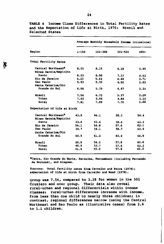
Income Class Differences in Fertility and Mortality

Socioeconomic differences in fertility and mortality areanother important dimension of recent Brazilian demo­graphic trends, though there are fewer data with which todocument them. Working with special tabulations of the1970 census, Carvalho and Paiva (1976) reported a differ­ential of over 4 children per woman in comparing totalfertility rates for high- and low-income families. Theirresults are summarized in the top half of Table 4. ForBrazil, total fertility in the 1-150 Cruziero per month

24

TABLE 4 Income Class Differences in Total Fertility Ratesand the Expectation of Life at Birth, 1970: Brazil andSelected States

AVeJ:llge Monthly Bou..hold Inco.e (cruzeiros)

Region 1-150 151-300 301-500 500+

J Total Fertility Rates

Central Northeasta 8.55 8.15 6.28 3.95Minas Gerais/Espirito

Santo 8.03 8.50 7.27 4.62Rio de Janeiro 6.23 5.43 4.40 2.71Sao Paulo 5.93 5.35 4.50 2.93Santa Catarina/Rio

Grande do SuI 6.08 5.79 4.97 3.25

Brazil 7.54 6.72 5.37 3.28Urban 7.03 5.95 4.84 3.10Rural 7.81 7.99 7.70 5.86

Bxpectation of Life at Birth

Central Northeasta 43.8 46.1 50.3 54.4Minas Gerais/Espirito

Santo 53.8 55.4 58.6 62.3Rio de Janeiro 54.1 54.8 57.6 62.1Sao Paulo 54.7 56.1 58.7 63.9Santa Catarina/Rio

Grande do SuI 60.5 61.2 63.4 66.9

Brazil 49.9 54.5 57.6 62.0Urban 46.0 53.7 57.6 62.2Rural 51.4 55.9 57.6 60.0

&Ceara, Rio Grande do Norte, Parnaiba, Pernaabuco (including Fernandode Noronha), and Alagoas.

Sources: Total fertility rates from Carvalho and Paiva (1976),expectation of life at birth from Carvalho and Wood (1978).

group was 7.54, compared to 3.28 for women in the 501Cruziero and over group. Their data also revealrural-urban and regional differentials within incomeclasses: rural-urban differences increase with income,from less than one child to nearly three children, incontrast, regional differences narrow (using the CentralNortheast and Sao Paulo as illustrative cases) from 2.6to 1.1 children.

25

Equally dramatic mortality differentials were found.Using the same tabulations, Carvalho and Wood (1978)noted a striking 20-year differential between the lifeexpectancy of low-income families in the Central North­east and that of high-income families in Sao Paulo, andan even greater difference when the Northeast was com­pared to the Southern states of Santa Catarina and RioGrande do Sul. Their results, summarized in the bottomhalf of Table 4, also suggest that for low-income house­holds, life expectancy was higher in rural than in urbanareas. However, caution is required in interpreting thisdifference since the income figures do not include incomein kind, which was higher in rural areas, thus the truelevel of living among these groups may have been under­stated. In contrast to the fertility differentials,regional differentials in mortality were maintained atabout 10 years as income increased, while rural-urbandifferences narrowed. Both sets of differentials high­light the importance of underlying socioeconomic variablesin the regional differentials observed during the 1950-70period, attention to changes in these variables willtherefore be important in explaining the acceleration inBrazil's fertility decline after 1970.

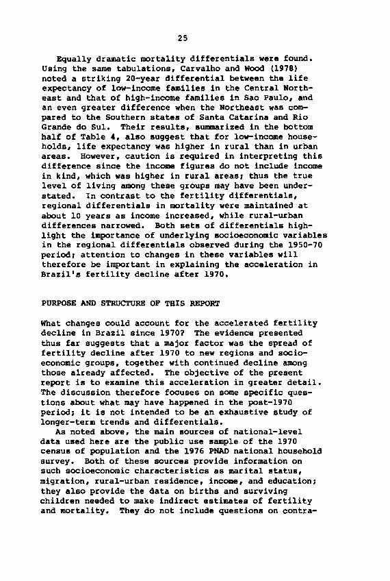
PURPOSE AND STRUCTURE OF THIS REPORT

What changes could account for the accelerated fertilitydecline in Brazil since 19701 The evidence presentedthus far suggests that a major factor was the spread offertility decline after 1970 to new regions and socio­economic groups, together with continued decline amongthose already affected. The objective of the presentreport is to examine this acceleration in greater detail.The discussion therefore focuses on some specific ques­tions about what may have happened in the post-1970period, it is not intended to be an exhaustive stUdy oflonger-term trends and differentials.

As noted above, the main sources of national-leveldata used here are the public use sample of the 1970census of popUlation and the 1976 PNAD national householdsurvey. Both of these sources provide information onsuch socioeconomic characteristics as marital status,migration, rural-urban residence, income, and education,they also provide the data on births and survivingchildren needed to make indirect estimates of fertilityand mortality. They do not include questions on contra-

26

ception and other proximate variables, nor are othernational-level survey data on these variables available.State-level data are found in reports of the Contracep­tive Prevalence Surveys (CPS) conducted by Brazil'sInternational Planned Parenthood Federation (IPPF)affiliate, Sociedade Civil Bem-Estar Familiar no Brasil(BEMFAM), with the cooperation of the u.S. Center forDisease Control, six such surveys were available when thereport was prepared (Sao Paulo, Piaui, Rio Grande doNorte, Pernambuco, Paraiba, and Bahia). Local case studydata on the proximate variables were assembled for theCentro Brasileiro de Analise e Planejament (CEBRAP)National Investigation on Human Reproduction (NIHR),which is examined in detail in Part II.

This study is organized as follows. Following thesummary, Part I concentrates primarily on national-leveldata. Chapter 1 uses national census and survey data onfertility and nuptiality, together with CPS state-leveldata on contraception, abortion, and breastfeeding, todecompose recent fertility declines into the proximatedeterminants of fertility, this analysis is based on thestandardization approach to decomposition of changes atthe national level. In Chapter 2, national data are usedto identify the level and amount of change in socio­economic fertility differentials from 1970 to 1976. Chap­ter 3 examines hypotheses about links between changes inthe proximate determinants and socioeconomic conditionsin Brazil during the early 1970s, as well as national­level empirical evidence relating to these hypotheses.Chapter 4 uses multivariate regression analysis toclarify links between changing socioeconomic conditionsand changes in average parity, with reference to theanalytical questions raised in the previous chapter.

Although Part I makes some reference to relevantlocal-level NIHR findings, its primary focus, as notedabove, is at the national level. Part II of this reportfocuses specifically on the NIHR to provide a more con­centrated analysis of Brazilian fertility. Chapter 5describes the purpose and methodology of the NIHR.Chapter 6 summarizes fertility levels and trends for thecontexts studied, which are described in detail in theAppendix. Chapter 7 presents a discussion of localtrends in nuptiality, including variations in union typeand age at marriage. Chapter 8 examines data related todeclining marital fertility, while Chapters 9 and 10analyze the role of the proximate determinants andsocioeconomic variables, specifically family income,

27

respectively, in that decline. Finally, Chapter 11presents some conclusions about Brazil's acceleratedfertility decline based on the NIHR data. It is hopedthat together, the broader and more focused persPeCtivesoffered in this report will provide a balancedunderstanding of Brazil's recent fertility trends.

PART I FERTILITY DETERMINANTS AT THE NATIONAL LEVEL

CHAPTER 1

THE PROXIMATE DETERMINANTS OF FERTILITY

The objective of this chapter is to analyze Brazil'saccelerated fertility decline in demographic terms.Demographic theory indicates that two sets of variablesare important: one is population composition, particu­larly age structure and marriage patterns, both of whichmediate the relation between individual reproductivebehavior and birth rates observed in a populationJ theother is comprised of the Davis-Blake (1956) -intermedi­ate variables,- such as frequency of intercourse,fertility control, breastfeeding, and abortion, whichdirectly affect reproductive outcome. This chapter usesa standardization approach to identify compositionaleffects, and Bongaarts' (1980) method for decomposingnatural fertility into its proximate determinants toidentify intermediate variables.

This chapter is based on the available data for Brazil,which are fragmentary in both regional and time coverage.The approach is therefore essential detective work, piec­ing together clues from a variety of sources in an attemptto draw a picture at the national level. Changes in mar­riage patterns and age structure are always prime suspectsin declining birth ratesJ therefore, the discussion beginsby assessing changes in the distribution of women by mar­ital status and in mean age at marriage, and then appliesstandardization techniques to check whether these changesand those in age structure played a major role in Brazil'sfertility decline. The available evidence suggests thatthey did not. This suggests in turn that the primaryfactor in the decline was one of the intermediate vari­ables affecting marital fertility. The Bongaarts frame­work is then used to explore this possibility. There arethree potential factors responsible--breastfeeding,contraception, and abortion. Among these, the limited

29

30

degree to which the first is practiced in Brazil issufficient to eliminate it as a primary influence. Theevidence implicating the second is stronger, thoughadmittedly fragmentary. Finally, although the evidenceis clearly circumstantial, it is strong enough toimplicate abortion as an imPOrtant, though necessarilyindeterminate, influence on Brazil's fertility decline.

MARITAL STATUS AND MEAN AGE AT MARRIAGE

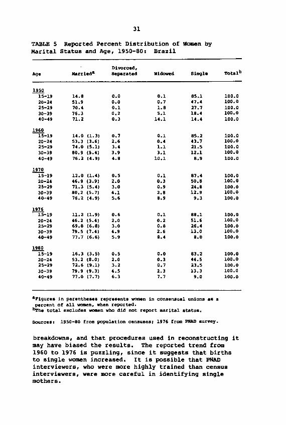
As noted above, the reporting of marital status inBrazilian data is problematic. The reported percentagedistribution of Brazilian women aged 15-49 by maritalstatus in the 1950, 1960, and 1970 censuses and in the1976 PNAD survey are presented in Table 57 preliminaryresults of the 1980 census are also reported. Fourmarital status categories are shown--married, divorcedand separated, widowed, and single. Each of thesecategories presents its own set of problems.

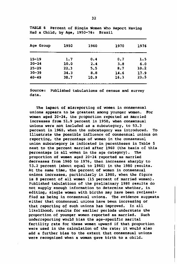
First, in the married category, there is a problem inthe reporting of women in consensual unions. Accordingto Henriques (1980), women in consensual unions accountfor an important share of Brazilian births, though Brazilhas a lower proportion of such births than a number ofother Latin American countries. However, althoughBrazilian data include women in consensual unions as asubcategory of married women, there is strong evidencethat a number of those who report themselves as singlemay in fact be in consensual unions (Silva, 1979:14).This is suggested by data in Table 6, which shows thepercent of women in the single category who reportedhaving had a birth from age 15-19 to 40-49 in thecensuses and PNAD survey.

Brazilian census authorities have attempted to improveon the reporting of consensual unions by broadening thenumber of categories of marital status to include thetype of union. In 1950, when there was no subcategoryfor consensual unions, nearly four out of ten singlewomen reported a birth by the end of their reproductiveyears, suggesting that most of these unions were groupedin the single category (Altmann and Wong, 1981a:356).This contrasts with 1960, when the consensual unioncategory was introduced and the proportion of singlewomen reporting a birth dropped to 11 percent. It shouldbe recalled that tabulation of the 1960 census wasdelayed until the late 1970s because of administrative

31

TABLE 5 Reported Percent Distribution of Women byMarital Status and Age, 1950-80: Brazil

Divorced,Tota1bAge Marrieda separated Widowed Single

.!lli.15-19 14.8 0.0 0.1 85.1 100.020-24 51.9 0.0 0.7 47.4 100.025-29 70.4 0.1 1.8 27.7 100.030-39 76.3 0.2 5.1 18.4 100.040-49 71.2 0.3 14.1 14.4 100.0

1960-r5"-19 14.0 (1.3) 0.7 0.1 85.2 100.0

20-24 53.3 (3.6) 2.6 0.4 43.7 100.025-29 74.0 (5.1) 3.4 1.1 21.5 100.030-39 80.9 (5.4) 3.9 3.1 12.1 100.040-49 76.2 (4.9) 4.8 10.1 8.9 100.0

197015-19 12.0 (1.4) 0.5 0.1 87.4 100.020-24 46.9 (3.9) 2.0 0.3 50.8 100.025-29 71.3 (5.4) 3.0 0.9 24.8 100.030-39 80.2 (5.7) 4.1 2.8 12.9 100.040-49 76.2 (4.9) 5.6 8.9 9.3 100.0

1976~-19 11.2 (1.9) 0.6 0.1 88.1 100.0

20-24 46.2 (5.4) 2.0 0.2 51.6 100.025-29 69.8 (6.8) 3.0 0.8 26.4 100.030-39 79.5 (7.4) 4.9 2.6 13.0 100.040-49 77.7 (6.6) 5.9 8.4 8.0 100.0

198015-19 16.3 (3.5) 0.5 0.0 83.2 100.020-24 53.2 (8.0) 2.0 0.3 44.5 100.025-29 72.6 (9.1) 3.2 0.7 23.5 100.030-39 79.9 (9.3) 4.5 2.3 13.3 100.040-49 77.0 (7.7) 6.3 7.7 9.0 100.0

aFigures in parentheses represents women in consensual unions as apercent of all women, when reported.

orhe total excludes women who did not report marital status.

Sources I 1950-80 from population censuses/ 1976 from PHAD survey.

breakdowns, and that procedures used in reconstructing itmay have biased the results. The reported trend from1960 to 1976 is puzzling, since it suggests that birthsto single women increased. It is possible that PNADinterviewers, who were more highly trained than censusinterviewers, were more careful in identifying singlemothers.

32

TABLE 6 Percent of Single Women Who Report HavingHad a Child, by Age, 1950-76: Brazil

Age Group 1950 1960 1970 1976

15-19 1.7 0.4 0.7 1.520-24 10.0 2.4 3.8 6.025-29 22.3 5.5 8.7 10.230-39 34.3 8.8 14.6 17.940-49 38.7 10.9 16.3 23.5

Source: Published tabulations of census and surveydata.

The impact of misreporting of women in consensualunions appears to be greatest among younger women. Forwomen aged 20-24, the proportion reported as marriedincreases from 51.9 percent in 1950, when consensualunions were not included as a subcategory, to 53.3percent in 1960, when the subcategory was introduced. Toillustrate the possible influence of consensual unions onreporting, the percentage of women in the consensualunion SUbcategory is indicated in parentheses in Table 5next to the percent married after 1960 (the basis of thispercentage is all women in the age category). Theproportion of women aged 20-24 reported as marrieddecreases from 1960 to 1976, then increases sharply to53.2 percent (about equal to 1960) in the 1980 results.At the same time, the percent of women in consensualunions increases, particularly in 1980, when the figureis 8 percent of all women (15 percent of married women).Published tabulations of the preliminary 1980 results donot supply enough information to determine whether, inediting, single women with births may have been reclassi­fied as being in consensual unions. The evidence suggestseither that consensual unions have been increasing orthat reporting of such unions has improved. In alllikelihood, results for earlier periods understate theproportion of younger women reported as married. Suchunder reporting would bias the age-specific maritalfertility rate for these women upward if that proportionwere used in the calculation of the rate, it would alsoadd a further bias to the extent that consensual unionswere recognized when a woman gave birth to a child.

33

Although the impact of the under reporting of consensualunions is reduced by grouping all single women with birthsin the married category, it is not eliminated. One isstill left with the problem of women in informal unionswho have no children, but should be included in thedenominator when fertility rates are calculated. Thisomission could bias calculation of rates for youngerwomen, particularly when the beginning of an informalunion is not clearly demarcated and the birth of a childleads to recognition (or admission) of the union.Including in the married category only those -single­women who had births will lead to overstatement ofmarital fertility rates. One way to compensate for thisis to assume that the proportion of single women -atrisk- is equal to that of married women, that is, if 50percent of married women aged 20-24 report a birth, thenassume that the single women aged 20-24 reporting a birthrepresent 50 percent of the single women at risk. Thisat-risk group can then be added to the married category.This procedure will be employed later in calculating thedenominators for marital fertility rates. The issue oftype of union and its relationship to fertility at thelocal level is explored in detail in Part II of thisreport.

A second problem of consistency in the Brazilian dataon marital status relates to the reporting of separatedand divorced women. Because Brazil legalized divorceonly in 1977, its effects cannot be observed directlyeven in the 1976 survey. However, reporting of foreigndivorces, legal separations, and a special Brazilianlegal substitute for pre-1977 divorces (desquites) wasincreasing in the years prior to actual legalization.The contrast is sharpest between 1950, when practicallyno divorces and separations were reported, and the otherdata points. Because divorce was not legally recognized,it was fairly common practice for women who had entered asecond union after separation to be declared as separatedrather than married, leading to further underreporting ofthe proportion of women in unions.

Such problems with the reliability of marital statusdata suggest that considerable caution is required in thecalculation and interpretation of measures incorporatingthose data. This applies not only to the proportion ofwomen in unions, but also to measures of the average ageat marriage and marital fertility rates. Table 7 sum­marizes the results of calculations of the singu1ate meanage at marriage (SMAM), which is based on the proportion

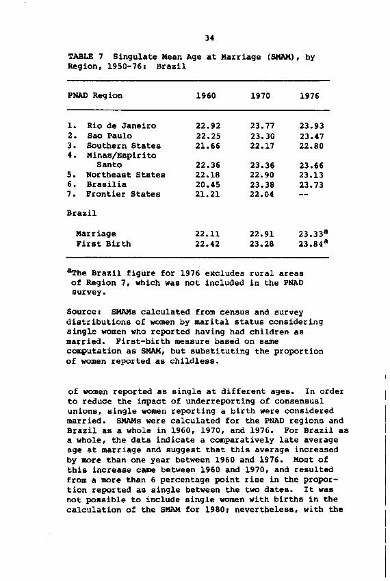
34

TABLE 7 Singulate Mean Age at Marriage (SMAM), byRegion, 1950-76: Brazil

PNAD Region

1. Rio de Janeiro2. Sao Paulo3. SOuthern States4. Minas/Espirito

Santo5. Northeast States6. Brasilia7. Frontier States

Brazil

1960 1970 1976

22.92 23.77 23.9322.25 23.30 23.4721.66 22.17 22.80

22.36 23.36 23.6622.18 22.90 23.1320.45 23.38 23.7321.21 22.04

MarriageFirst Birth

22.1122.42

22.9123.28

~he Brazil figure for 1976 excludes rural areasof Region 7, which was not included in the PNADsurvey.

Source: SHAMs calculated from census and surveydistributions of women by marital status consideringsingle women who reported having had children asmarried. First-birth measure based on samecomputation as SMAM, but SUbstituting the proportionof women reported as childless.

of women reported as single at different ages. In orderto reduce the impact of underreporting of consensualunions, single women reporting a birth were consideredmarried. SMAMs were calculated for the PNAD regions andBrazil as a whole in 1960, 1970, and 1976. For Brazil asa whole, the data indicate a comparatively late averageage at marriage and suggest that this average increasedby more than one year between 1960 and 1976. Most ofthis increase came between 1960 and 1970, and resultedfrom a more than 6 percentage point rise in the propor­tion reported as single between the two dates. It wasnot possible to include single women with births in thecalculation of the SHAM for 1980, nevertheless, with the

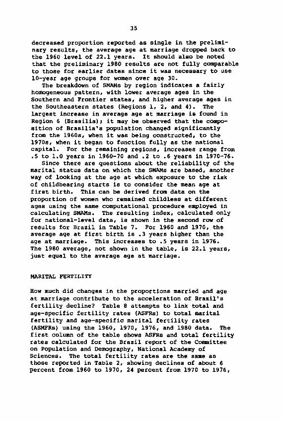
35

decreased proportion reported as single in the prelimi­nary results, the average age at marriage dropped back tothe 1960 level of 22.1 years. It should also be notedthat the preliminary 1980 results are not fully comparableto those for earlier dates since it was necessary to use10-year age groups for women over age 30.

The breakdown of SMAMs by region indicates a fairlyhomogeneous pattern, with lower average ages in theSouthern and Frontier states, and higher average ages inthe Southeastern states (Regions 1, 2, and 4). Thelargest increase in average age at marriage is found inRegion 6 (Brasilia), it may be observed that the compo­sition of Brasilia's population changed significantlyfrom the 1960s, when it was being constructed, to the1970s, when it began to function fUlly as the nationalcapital. For the remaining regions, increases range from.5 to 1.0 years in 1960-70 and .2 to .6 years in 1970-76.

Since there are questions about the reliability of themarital status data on which the SMAMs are based, anotherway of looking at the age at which exposure to the riskof childbearing starts is to consider the mean age atfirst birth. This can be derived from data on theproportion of women who remained childless at differentages using the same computational procedure employed incalculating SHAMs. The resulting index, calculated onlyfor national-level data, is shown in the second row ofresults for Brazil in Table 7. For 1960 and 1970, theaverage age at first birth is .3 years higher than theage at marriage. This increases to .5 years in 1976.The 1980 average, not shown in the table, is 22.1 years,just equal to the average age at marriage.

MARITAL FERTILITY

How much did changes in the proportions married and ageat marriage contribute to the acceleration of Brazil'sfertility decline? Table 8 attempts to link total andage-specific fertility rates (ASFRs) to total maritalfertility and age-specific marital fertility rates(ASMFRs) using the 1960, 1970, 1976, and 1980 data. Thefirst column of the table shows ASFRs and total fertilityrates calculated for the Brazil report of the Committeeon Population and Demography, National Academy ofSciences. The total fertility rates are the same asthose reported in Table 2, showing declines of about 6percent from 1960 to 1970, 24 percent from 1970 to 1976,

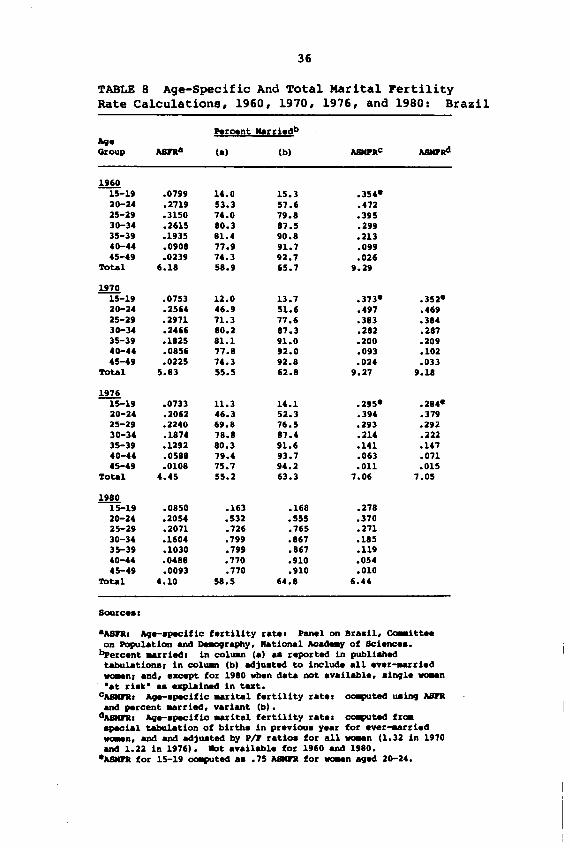
36

TABLE 8 Age-Specific And Total Marital FertilityRate Calculations, 1960, 1970, 1976, and 1980: Brazil

Percent MarriedbAgeGroup A8fta (a) (b) ASIIFRc ABIlI'ad

1960-U-19 .0799 14.0 15.3 .354e

20-24 .2719 53.3 57.6 .47225-29 .3150 74.0 79.8 .39530-34 .2615 80.3 87.5 .29935-39 .1935 81.4 90.8 .21340-44 .0908 77.9 91.7 .09945-49 .0239 74.3 92.7 .026

Total 6.18 58.9 65.7 9.29

197015-19 .0753 12.0 13.7 .373e .352e20-24 .2564 46.9 51.6 .497 .46925-29 .2971 71.3 77.6 .383 .38430-34 .2466 80.2 87.3 .282 .28735-39 .1825 81.1 91.0 .200 .20940-44 .0856 77.8 92.0 .093 .10245-49 .0225 74.3 92.8 .024 .033

Total 5.83 55.5 62.8 9.27 9.18

1976--u-19 .0733 11.3 14.1 .295e .284e

20-24 .2062 46.3 52.3 .394 .37925-29 .2240 69.8 76.5 .293 .29230-34 .1874 78.8 87.4 .214 .22235-39 .1292 80.3 91.6 .141 .14740-44 .0588 79.4 93.7 .063 .07145-49 .0108 75.7 94.2 .011 .015

Total 4.45 55.2 63.3 7.06 7.05

ill!15-19 .0850 .163 .168 .27820-24 .2054 .532 .555 .37025-29 .2071 .726 .765 .27130-34 .1604 .799 .867 .18535-39 .1030 .799 .867 .11940-44 .0488 .770 .910 .05445-49 .0093 .770 .910 .010

Total 4.10 58.5 64.8 6.44

Sourcee.

aUD. A9_epeeific fertility rate. Panel on Braail, ee-itt..on Population and oe.ography, Rational Acade.)' of SCiencee.

bpercent _uie,h in coluan (a) ae reported in publiehedtabulations, in coluan (b) adjueted to include all ever-aarried_n, and, except for 1980 vben data not available, single _n"at riek" ae explained in text.

cASIIFR. A9_epeeific _rital fertility rate. CCII(lUted ueing A8ftand percent _uied, variant (b).

dASIIFR. A9_epeeific ~ital fertility rate. CCII(lUted frcaepeeial tabulation of birthe in previoue year for ever-aarried_n, and and adjuated by PIP ratios for all _n (1.32 in 1970and 1.22 in 1976). lOt available for 1960 and 1980.

eASIIFR for 15-19 CCII(lUted ae .75 ASIIFR for _n aged 20-24.

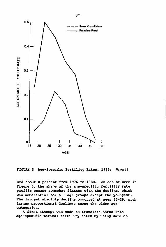
37

0.5_ _ _ santa Cruz-Urban

_ Parnaiba-Rural

0.4

wl-e(a:>-I- 0.3...J

i=a:wLL

ULL

u0.2 I'w

Q.. I ,(I)

wI '

C)e( I \

I \0.1 I \

/ \/ \

/ \....................

015 20 25 30 35 40 45 50

AGE

FIGURE 5 Age-Specific Fertility Rates, 1975: Brazil

and about 8 percent from 1976 to 1980. As can be seen inFigure 5, the shape of the age-specific fertility rateprofile became somewhat flatter with the decline, whichwas substantial for all age groups except the youngest.The largest absolute decline occurred at ages 25-29, withlarger proportional declines among the older agecategories.

A first attempt was made to translate ASFRs intoage-specific marital fertility rates by using data on

38

marital status from published reports, as shown in column(a) under -percent married- in Table 8. Because of theunderreporting of women in consensual unions, ASMFRsappear to be biased upward, particularly for women intheir twenties. In 1970, for example, the ASMPR for the20-24 group would be .547, this would mean that thefertility of Brazilian women exceeded that of the Hutter­ites, one of the populations on whose experience standardnatural fertility schedules are based. To reduce thisbias, the proportion -married- was adjusted to includeall ever-married women, single women who reported abirth, and a prorated number of single women -at risk­based on the proportion of married women reporting abirth, as shown in column (b) under -percent married- inthe table. This adjustment raised the percent married byabout 7 percentage points for each observation, althoughthis did not reduce the decline of about 5 percentagepoints in the proportion married among women 20-24 between1960 and 1970, it did narrow the differences between1970, 1976, and 1980. The increase in the proportionmarried among women in older age categories arises fromthe addition of widowed, separated, and divorced women.

Even with these adjustments, the ASMPRs and totalmarital fertility rates for 1960 and 1970 are quitehigh--nearly 9.3 for both dates. By 1976, total maritalfertility falls to 7.06, a decline of 24 percent, with afurther decline of 9 percent to 6.44 in 1980. Whiletotal marital fertility shows little change between 1960and 1970, the rate for women aged 20-24 increases. Thisoccurs because the decline in the ASFR for that group isless than the decline in the proportion married, evenafter adjustment. The rate for women aged 15-19 issimilarly affected since it was calculated as .75 of therate of those aged 20-24. Because these rates are sohigh, total marital fertility is very sensitive to suchdifferences, which are as likely to be the result ofdifferences in reporting (or editing, as suggested above)as they are to be real. Thus considerable caution isrequired in interpreting the 1960-70 period.

Access to pUblic use sample files for the 1970 and1976 data made it possible to tabulate the observednumber of births by marital status in the year prior tointerviews, this provided a check on the rates calculatedfrom ASFRs. Observed births were adjusted by the P/Fratios used in adjusting ASFRs for that date. Theresulting ASMPRs and total marital fertility rates areshown in the last column of Table 8. These rates are not

39

exactly comparable to those calculated directly fromASFRs since the adjustment of observed births used inderiving ASFRs also included a factor to account for theone-half-year difference between women's reported age andtheir age when births actually occurred. Because it isinappropriate to apply this factor when the denominatoris limited to ever-married women, the age profiles ofASMFRs differ with the two approaches. The main differ­ence is that rates based on the tabulations are lower forwomen under 25 and higher for women over 30. Total mar­ital fertility is slightly lower in 1970 and virtuallythe same in 1976 in the tabulated results. Comparison ofthe two sets of rates suggests that the decline in mar­ital fertility probably was close to 24 percent over the1970-76 period, however, there is a need to be cautiousabout both the level and age profile of marital fertilityrates.

The age category most seriously affected is 20-24.Two factors could account for an overstatement of theage-specific marital fertility rate for this group. Oneis the underreporting of married women discussed above.The other is that the adjustment factors derived usingthe Brass technique may be too high for this group.Estimates of ASMFRs using model marital fertilityschedules suggest that this may in fact be the case (seeBerquo and Leite, 1979, Altmann and Wong, 1981a, Leite,1981). One way to visualize the extent of possible biasis to compare observed ASMPRs to model schedules, asshown in Figure 6. Both of the 1970 ASMFR schedules fromTable 8 are plotted against these model schedules. Themodels are based on a total marital fertility rate of9.25, with the Coale-Trussel index of fertility controlset at three levels: 0.0, the natural fertility level,and 0.3 and 0.5, indicating moderate fertility control.The model schedule with the index set at 0.5 provides avery close approximation to both of the observed 1970ASMFR schedules for ages 25-29 to 40-44. The observedrates for age 20-24 exceed the model schedule, though thesecond schedule (estimated from births reported for-married- women, broadly defined) is closer than the ratecalculated from dividing ASFRs by the proportion married.The comparison suggests that the 1970 base for calcu­lating declines between 1970 and 1976 among the youngerage groups may be too high, resulting in an exaggerationof declines for women in these age categories.

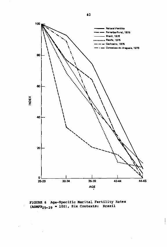
40

xwoz

80

80

40

20

- N8tur81 F8rtllitv

-- P8rlllllb8-Rur81.1976

-- Brull. 1976

•••••••• Recif.,1976

--- c.ehoeiro, 1976

- • - Col1C8ia10 do Ar8QU818, 1976

44-454D-4435-39

AGE,

30-34

Ol.....-- -'- ....L... .l.- .J

25-29

PIGURE 6 Age-Specific Marital Pertility Rates(ASMPR25-29 • 100), Six contexts: Brazil

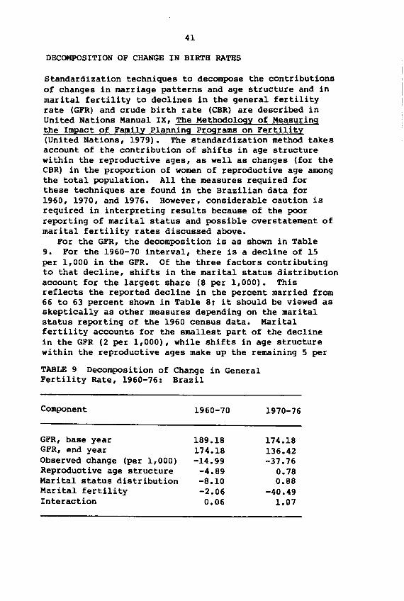
41

DECOMPOSITION OF CHANGE IN BIRTH RATES

Standardization techniques to decompose the contributionsof changes in marriage patterns and age structure and inmarital fertility to declines in the general fertilityrate (GFR) and crude birth rate (CBR) are described inUnited Nations Manual IX, The MethodologY of Measuringthe Impact of Family Planning Programs on Fertility(United Nations, 1979). The standardization method takesaccount of the contribution of shifts in age structurewithin the reproductive ages, as well as changes (for theCBR) in the proportion of women of reproductive age amongthe total population. All the measures required forthese techniques are found in the Brazilian data for1960, 1970, and 1976. However, considerable caution isrequired in interpreting results because of the poorreporting of marital status and possible overstatement ofmarital fertility rates discussed above.

For the GFR, the decomposition is as shown in Table9. For the 1960-70 interval, there is a decline of 15per 1,000 in the GFR. Of the three factors contributingto that decline, shifts in the marital status distributionaccount for the largest share (8 per 1,000). Thisreflects the reported decline in the percent married from66 to 63 percent shown in Table 8; it should be viewed asskeptically as other measures depending on the maritalstatus reporting of the 1960 census data. Maritalfertility accounts for the smallest part of the declinein the GFR (2 per 1,000), while shifts in age structurewithin the reproductive ages make up the remaining 5 per

TABLE 9 Decomposition of Change in GeneralFertility Rate, 1960-76: Brazil

Component

GFR, base yearGFR, end yearObserved change (per 1,000)Reproductive age structureMarital status distributionMarital fertilityInteraction

1960-70

189.18174.18-14.99

-4.89-8.10-2.060.06

1970-76

174.18136.42-37.76

0.780.88

-40.491.07

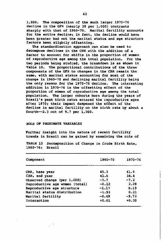
42

1,000. The composition of the much larger 1970-76decline in the GFR (nearly 38 per 1,000) contrastssharply with that of 1960-70. Marital fertility accountsfor the entire declineJ in fact, the decline would havebeen greater had not the marital status and age structurefactors been slightly offsetting.

The standardization approach can also be used todecompose declines in the CBR with the addition of afactor to account for shifts in the proportion of womenof reproductive age among the total population. For thetwo periods being studied, the breakdown is as shown inTable 10. The proportional contributions of the threecomponents of the GFR to changes in the CBR remain thesame, with marital status accounting for most of thechange in 1960-70 and declining marital fertility beingthe only reason for the 1970-76 decline. The interestingaddition in 1970-76 is the offsetting effect of theproportion of women of reproductive age among the totalpopulation. The larger cohorts born during the years ofBrazil's peak birth rates entered the reproductive agesafter 1970J their impact dampened the effect of thedecline in marital fertility on the birth rate by about afourth--2.3 out of 9.7 per 1,000.

ROLE OF PROXIMATE VARIABLES

Further insight into the nature of recent fertilitytrends in Brazil can be gained by examining the role of

TABLE 101960-76:

Decomposition of Change in Crude Birth Rate,Brazil

Component

CBR, base yearCBR, end yearObserved change (per 1,000)Reproductive age women (total)Reproductive age structureMarital status distributionMarital fertilityInteracticm

1960-70

45.341.6-3.7-0.12-1.17-1.93-0.49+0.01

1970-76

41.634.4-7.2

2.280.190.21

-9.72+0.30

43

the proximate variables identified in the Davis-Blake(1956) framework, and more recently in Bongaarts' (1980)

method for decomposing the difference between naturalfertility and observed total fertility rates into fourproximate determinants. Bongaarts' technique involvesthe computation of four indices: (1) em • the index ofthe proportion married, which equals one if all women ofreproductive age are married, zero if none are, (2)Cc • the index of noncontraception, which equals one inthe absence of contraception and zero if all women use100 percent effective contraception, (3) Ca • the indexof abortion, which equals one in the absence of inducedabortion and zero if all pregnancies are aborted, and (4)Ci = the index of postpartum infecundability, whichequals one in the absence of lactation and postpartumabstinence and zero if the duration of infecundability isinfinite. Observed total fertility is linked to naturalfertility (the number of births a women would have duringher reproductive lifetime if none of the inhibitingfactors were operative) by multiplying the number ofbirths that would occur in a natural-fertility regime byeach of the indices in succession: TFR· 15.3 x Cm xCa x Cc x Ci' where 15.3 represents an estimate ofthe total fecundity rate. It should be noted that theuse of a single value to estimate the fecundability levelof a population, set at 15.3 children per woman, has beenquestioned in light of the heterogeneity of populationsin relation to a number of factors, such as state ofhealth, duration of cohabitation, and so on. Thus, othervalues have been proposed for use in estimating thisparameter for specific population subgroups (seeLesthaeghe et al., 1981 and Gaisie, 1981). In thisreport, however, 15.3 will be used.

Data requirements for calculating the four indices aregeared to national-level fertility surveys, such as theWorld Fertility Survey, which inClude questions on breast­feeding and abortion as well as current contraceptive use.Census and survey data do provide enough information forcalculation of the marriage index, which is the ratio ofthe total fertility rate to the total marital fertilityrate, and which remained constant at a level of .63 from1970 to 1976. In the absence of any nationally repre­sentative Brazilian data on the three remaining variables,the best that can be done is to piece together a national-guesstimate- from the fragments of subnational surveydata that are available.

44

The two main sources of survey data for the 1970s arethe local-level CEBRAP National Investigation on HumanReproduction (NIBR) and the state-level ContraceptivePrevalence Surveys (CPS), mentioned in Chapter 1. TheNIBR interviews were conducted during 1975 in the statesof Sao Paulo, Espirito Santo, Rio Grande do SuI,Pernambuco, Piaui, and Para (Berquo, 1976). The firstCPS was conducted in Sao Paulo in 1978, followed by Piauiin 1979, and Pernambuco, Rio Grande do Norte, Paraiba,and Bahia in 1980 (Rodrigues et al., 1981a). Additionalsurvey work was being conducted in Southern Brazil in1981. Prior to these inquiries, the data were limited toa handful of surveys in specific localities: Rio deJaneiro was included in the comparative study of fertilityand family planning in nine Latin American cities con­ducted by CELADE in 1963 (CELADE, 1972), and CEBRAPinterviewed women in the municipality of Sao Paulo in1965 (Berquo et al., 1977a)J two other surveys includeMartine's 1969 interviews of poor women who were usingthe services of a maternity clinic in Rio de Janeiro(Martine, 1975) and Etges' survey of women in PortoAlegre and two other localities in Rio Grande do SuI in1973 (Etges, 1975). The subsections that follow assembleinformation on current contraceptive use, abortion, andbreastfeeding from these surveys in a form that willpermit calculation of the Bongaarts' indices.

Contraceptive Use

The index of noncontraception requires information on thepercent of fecund married women of reproductive age cur­rently using contraception, as well as a breakdown ofmethods by type to measure contraceptive effectiveness(Bongaarts, 1980). The available national-level Braziliandata are summarized in Table llJ as noted in Chapter 9,these data are paralleled by local-level NIBR data. The1965 Sao Paulo survey is reported (Nakamura et al., 1979)to indicate that 66 percent of eligible women were usingcontraception, a higher proportion than was reported forRio de Janeiro (38 percent) a year earlier. However, itis not apparent from reports on the Sao Paulo survey(Berquo et al., 1977a) whether the figure refers tocurrent or ever useJ if it is the latter, then 66 percentprobably overstates current use. Both surveys indicatethat methods other than the pill and sterilization werepredominant. Martine's 1969 data on poor women in Rio

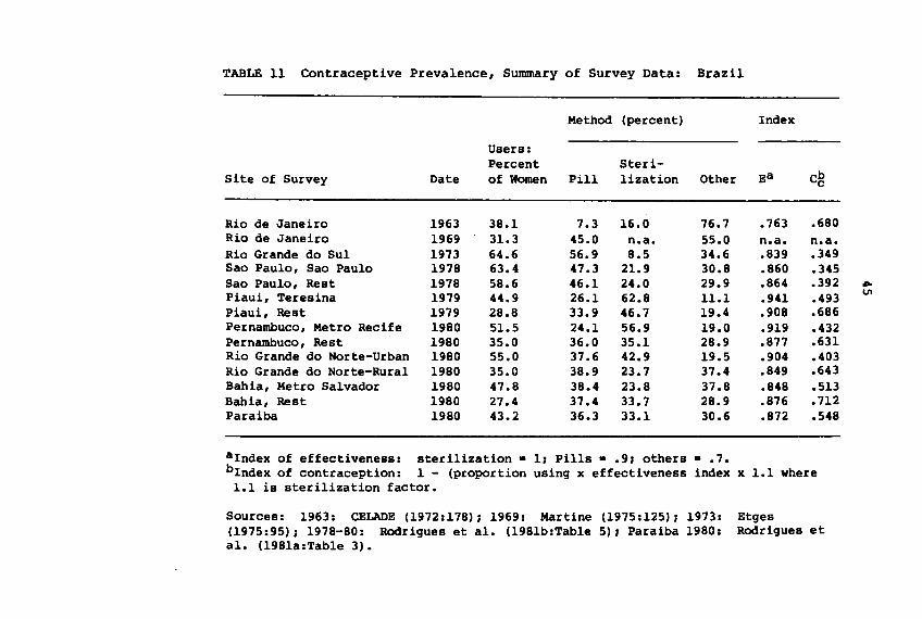
TABLE 11 Contraceptive Prevalence, Summary of Survey Data: Brazil

Method (percent) Index

Site of Survey Date

Users:Percentof Women Pill

Steri-lization Other Ea Cbc

Rio de JaneiroRio de JaneiroRio Grande do SulSao Paulo, Sao PauloSao Paulo, RestPiaui, TeresinaPiaui, RestPernambuco, Metro RecifePernambuco, RestRio Grande do Norte-UrbanRio Grande do Norte-RuralBahia, Metro SalvadorBahia, RestParaiba

19631969197319781978197919791980198019801980198019801980

38.131.364.663.458.644.928.851.535.055.035.047.827.443.2

7.345.056.947.346.126.133.924.136.037.638.938.437.436.3

16.0n.a.8.5

21.924.062.846.756.935.142.923.723.833.733.1

76.755.034.630.829.911.119.419.028.919.537.437.828.930.6

.763n.a..839.860.864.941.908.919.877.904.849.848.876.872

.680n.a .• 349.345.392.493.686.432.631.403.643.513.712.548

..VI

aIndex of effectiveness: sterilization. IJ Pills • .9J others· .7.bIndex of contraception: 1 - (proportion using x effectiveness index x 1.1 where1.1 is sterilization factor.

Sources: 1963: CELADE (1972:178)J 1969: Martine (1975:125)J 1973:(1975:95)J 1978-80: Rodrigues et al. (1981b:Table 5)J Paraiba 1980:al. (1981a:Table 3).

EtgesRodr igues e t

46

indicate a sharp rise in pill use in the late 1960s,however, his survey is not comparable with the otherssince it did not include women who had been sterilized.The data on Rio Grande do Sul also show increased use ofthe pill, as well as a contraceptive use rate of nearly65 percent.

The 1978 Sao Paulo CPS indicated that 63 percent ofcurrently married women aged 15-44 were using contracep­tives in the city of Sao Paulo, a figure slightly lowerthan that cited in the survey taken a decade earlier.Even if current use really was 66 percent in 1965, the1978 survey indicates an important increase in effectivecontraception because of a shift to more effectivemethods, with the pill and sterilization accounting fornearly two-thirds of users in 1978 comPared to less thanone-fifth in 1965. The 1978 survey also indicated thatcontraceptive use was nearly as high in the rest of SaoPaulo, including rural areas, as it was in the capitalcity. The second CPS survey, conducted in 1979, shiftedfro. Brazil's most developed to its least developedstate, Piaui. Current users accounted for 45 percent ofwomen in the capital city of Teresina and 29 percent inthe rest of the state, which is predominantly rural. Themost noteworthy feature of the Piaui data is the verymajor role played by sterilization, which represented 63percent of all fertility control, the figure for the restof the state was 47 percent. The 1980 Pernambuco and RioGrande do Norte surveys tell a similar story: over 50percent of women in Recife were currently using a method,with sterilization accounting for 57 percent of thetotal, in urban Rio Grande do Norte, sterilization andthe pill were used in equal proportions. Finally, itshould be noted that prevalence rates in general werehigher in the rural areas of these states than in Piauiand Bahia, a reflection of the impact of community-basedfamily planning programs organized by BEMFAM in coopera­tion with state governments (Rodrigues et al., 1981a).

The last two columns of figures in Table 11 provideestimates of the index of noncontraception (Cc ) foreach of the surveys for which the needed information wasavailable. Computations were based on Bongaarts' formula:Cc ~ 1 - (S x E x U), where ·S· is a correction factorfor sterility, ·E· is a measure of average contraceptiveeffectiveness based on the share of each method in thetotal, and ·U· is the proportion of married women cur­rently using a method. The sterility correction factorwas set at 1.1, Bongaarts' recommendation for less

47

developed areas. Values of U were taken from the columnshowing the percent of current users. The value of E wasdetermined from the three columns showing percent of totaluse for pills, sterilization, and other methods, witheffectiveness ratings of 1.0, 0.9, and 0.7, respectively.Index values for the late 1970s range from about .35 forSao Paulo to .70 for Bahia state, eXClusive of Salvador.

The information in Table 11 falls far short of what isrequired to compute values of the index of noncontracep­tion for Brazil during the 1970s. Most of the informa­tion relates to the later years of the decade, and only afraction of the total population is represented. At best,these data are a rough guide to the extent of regionaldifferentials, and serve as a basis for guesses at whatthe trends may have been. For illustrative purposes,they have been used to calculate national-level estimatesof the index for three dates (1970, 1976, and 1980). Thefirst step in making such calculations was to determinevalues for S, E, and U for the three dates, as shown inTable 12. National-level estimates of these measureswere derived as follows. The sterilization index wasassumed not to vary by region, and was set at 1.1 in1970, then raised to 1.125 as the prevalence of steril­ization increased. Values of U and E were assigned toeach of six subdivisions of the Brazilian population,which was broken down by region (Northeast, South andSoutheast, and North and Central-West) and by rural-urbanresidence. Those assignments were based on speculationabout levels of these measures that would be consistentwith the fragmentary trends suggested by the survey data.

For 1970, effectiveness was assumed to vary from .75in the rural North and Northeastern regions to .85 in theurban Southeast. It was assumed that E converged on .90for urban areas and on .85 for rural areas in 1980 ascontraceptive use spread. The user rate was assumed torange from .05 for the rural North and Northeast to .55in the urban Southeast in 1970, and was increased to .35and .60 for the 1980 assumptions. It should be stressedagain that these are merely illustrative figuresJ theyare based on speculation about possible regional patternsof contraceptive use and effectiveness derived from thefragmentary evidence presented in Table 11. Actualnumbers on which to base such an assessment simply do notexist. These illustrative figures will be incorporatedbelow in the calculation of overall national-levelestimates of the proximate determinants of fertility oncesimilar speculative estimates of the prevalence ofabortion and breastfeeding have been described.

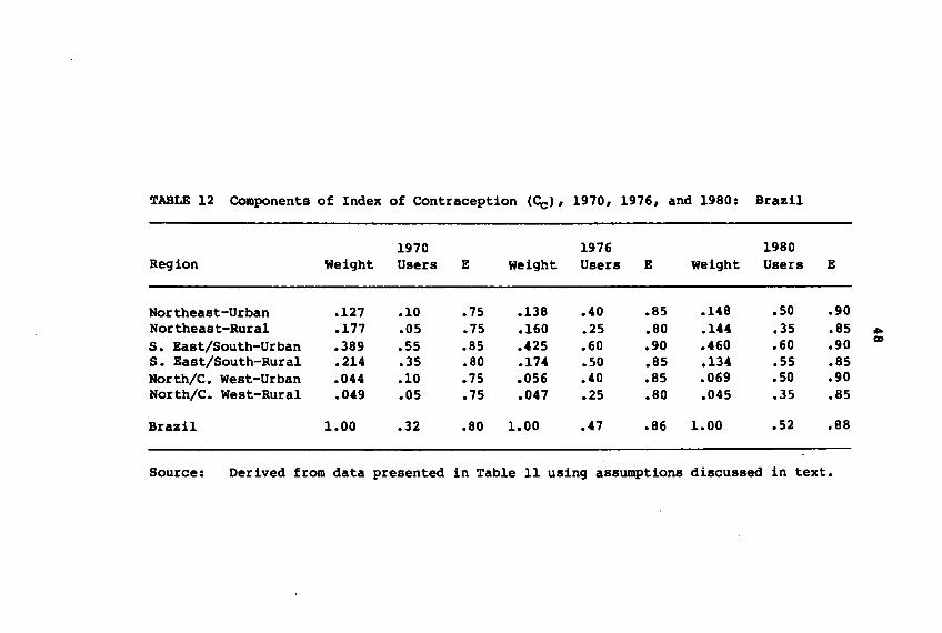
TABLE 12 Components of Index of COntraception <ce), 1970, 1976, and 1980: Brazil

1970 1976 1980Region Weight Users E weight Users E weight Users E

Northeast-Urban .127 .10 .75 .138 .40 .85 .148 .50 .90Northeast-Rural .177 .05 .75 .160 .25 .80 .144 .35 .85 ..S. East/South-Urban .389 .55 .85 .425 .60 .90 .460 .60 .90 Cll)

S. East/South-Rural .214 .35 .80 .174 .50 .85 .134 .55 .85North/C. West-Urban .044 .10 .75 .056 .40 .85 .069 .50 .90North/C. West-Rural .049 .05 .75 .047 .25 .80 .045 .35 .85

Brazil 1.00 .32 .80 1.00 .47 .86 1.00 .52 .88

Source: Derived from data presented in Table 11 using assumptions discussed in text.

49

Abortion

Abortion is illegal in Brazil, and the Brazilian penalcode carries a sanction of several years of imprisonmentat hard labor for both abortionists and women who practiceit (Milanesi, 1970:12-13). However, the code is rarelyinvoked, except as a legal ploy in such efforts as theattempt to block the importation and use of the IUD as an-abortifacient.- Abortion is believed to be widespread,rates of mortality and hospitalization resulting fromabortion-related infections are high, though not welldocumented.

There are no reliable statistical data on abortions atthe national level in Brazil, though there are reportedestimates (based on some rather implausible extrapola­tions from the experience of hospitals in a few local­ities). According to these estimates, the annual numberof abortions runs as high as three million per year,which would mean eight abortions for every ten livebirths (Rodrigues et al., 1975, Carvalho et al., 1981).The hard evidence that does exist suggests that poor,urban, and noncontracepting women are more likely toresort to induced abortion, and that only a fraction ofthese women identify themselves when the question isasked in survey interviews. Martine (1975) suggests thatanother reason for low observed abortion rates is thehigh mortality rate among women having abortions who, asa consequence, would not be accounted for. Questions onabortion have been asked in a number of fertility surveysconducted in Brazil since the early 1960s, including theNIHR and CPS, these provide a basis for calculation ofthe abortion index.

The way the incidence of abortion is reported variesby survey. Por purposes of calculating Bongaarts' indexof the effect of abortion on fertility, the ideal wouldbe the total induced abortion rate, this is analogous tothe total fertility rate and indicates the number ofabortions a woman would have during her reproductivelifetime if current rates prevailed. Either annualage-specific abortion rates or the total number ofabortions for women who have completed their reproductivelife cycle could be used to calculate such a rate. How­ever, samples are rarely large enough to give reliableestimates by the first method, and in only a few of theBrazilian studies are rates broken down by age. Varia­bility in measures affects both the numerators anddenominators of rates. In some cases, numerators refer

50

to induced abortion, in others to all abortions (spontane­ous and induced)J some numerators indicate the number ofabortions, others the number of women ever having had anabortion. Denominators include the number of women ofreproductive age (usually restricted to women in unions)and/or the total number of pregnancies reported by theseWaDen.

Table 13 summarizes available statistical informationon abortion in Brazil. Hutchinson's data on Rio deJaneiro in 1963 indicate that 9 percent of married womenof reproductive age had experienced an abortion, while a1965 CBBRAP study of Sao Paulo reveals that 18 percent ofpregnancies ended in abortions, about one-third of whichwere induced. Martine's data on poor women in Rio deJaneiro in 1969 suggest a sUbstantially higher incidenceof abortion among low-incaDe groups. Etges' study ofthree aunicipalities in Rio Grande do Sul in 1973 shows ahigher rate of induced abortions as a percent of allpregnancies in Porto Alegre than in two smaller municipal­ities that he sa.pled. Questions on abortion have beenincluded in all six of the CPSs for which tabulations areavailable. WaDen were asked how many abortions (spontane­ous and induced) they had experienced, and whether theirlast abortion was spontaneous or induced. The proportionof induced abortions in the 1978 Sao Paulo survey wasmuch lower (closer to one-ninth) than the one-third figureof the 1965 Sao Paulo surveYJ this suggests (1) thatinduced abortion is underreported in the CPS data, and/or(2) that a higher level of contraceptive use in 1978 mayhave resulted in a substitution of contraception forabortion (Nakamura et al., 1979117). The proportion ofWaDen reporting having had an induced abortion was higherin urban areas of Sao Paulo. In other CPSs, the propor­tion of~ reporting that they had ever had an abortionwas higher in rural areas, but the proportion of ~­nancies ending in abortion was higher in urban areas.CPS abortion data have been tabulated by women's ageJthis peraitted a rough approximation of the total abortionrate, which was calculated as the proportion of thedifference between the total pregnancy rate and the totalfertility rate that could be attributed to inducedabortion. This difference averaged .57 per woman in theNortheast, where the total fertility rate was 6.3 perwoman. If the reported 10-15 percent share of inducedabortion were accepted, the total abortion rate would bea very low .06 to .08 per womanJ if all reported termina­tions of pregnancy were attributed to induced abortion,

51

then the total induced abortion rate would be .57 perwoman.

Berquo (1980) has calculated total abortion rates forthe nine localities included in the NIHR survey. Theserange from .068 abortions per woman in Santa Cruz-Urbanin the state of Rio Grande do Sul to .735 in Parnaiba­Rural in the state of Piaui. There is no consistentrural-urban pattern, though there is a suggestion thatabortion rates are higher in larger cities and in poorerregions. It is also possible to speculate on totalabortion rates using CPS data on the proportion ofpregnancies ending in abortion. In Salvador, Bahia, forexample, assuming that one-third of reported abortionsare induced and the total fertility rate is about 4, thetotal induced abortion rate would be about .2 per woman:for Bahia-Rural, with a total fertility rate of 7, thetotal abortion rate is about the same. For Recife,calculation based on a total fertility rate of 4 yieldsan abortion rate of .25 per woman, about half of the rateindicated in the NIHR data: this is again consistent withthe interpretation that (1) the CPSs underreport abortionmore than does the NIHR survey, and/or (2) increasedcontraceptive use is being substituted for abortion.

The Bongaarts index for measuring the effect ofabortion on the fertility rate is defined by theexpression

Ca

= --=T;.;;F;.;;R~ _TFR + 0.4 (l+u) TAR

where ·u· is the parameter already estimated when calcu­lating the contraception rate. Ca becomes zero if allpregnancies are aborted, and is equal to 1 if all aresuccessful. In applying this index to recent Brazilianfertility trends, one can at best speculate on orders ofmagnitude suggested by these survey results for the totalinduced abortion rate. There are several qualificationsto be noted here. First, it is very likely that thesurvey data presented above greatly understate the abor­tion rate. Second, in addition to showing the prevalenceof abortion, variation in Bongaarts' abortion index alsoreflects the level of fertility and of contraceptive use(to the extent that both, in turn, are related to thepotential number of pregnancies to be aborted). Thusabortion, contraception, and fertility must be balancedin any calculations. Finally, uncertainty about thelevel of the abortion rate also relates to the impact of

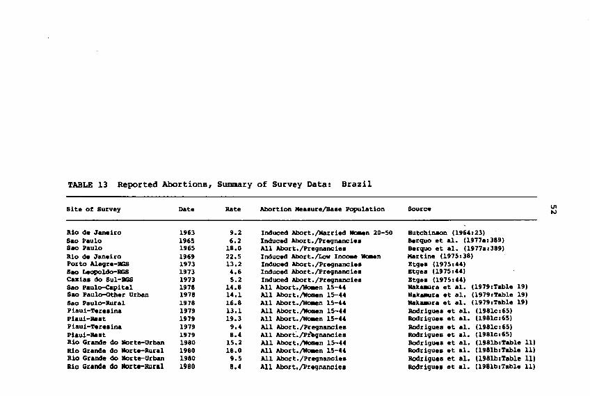
TABLE 13 Reported Abortions, Summary of Survey Data: Brazil

Site of Survey Date Rate Abortion Mea.ure/Ba.e Population Source VIN

Rio de Janeiro 1963 9.2 Induced Abort./Married wo.en 20-50 Butchinaon (196~:23)

Sao Paulo 1965 6.2 Induced Abort./Pregnancie. Berquo et a1. (1977a:389)Sao Paulo 1965 18.0 All Abort./Preqnancie. Berquo et a1. (1977a:389)Rio de Janeiro 1969 22.5 Induced Abort./Low IIlCOIMI wo.en Martine (1975:38)Porto Alegre-RGS 1973 13.2 Induced Abort./Pregnancie. Btqes (1975:44)Sao Leopoldo-RGS 1973 ~.6 Induced Abort./pregnancie. Btqes (1975:44)Casias do Su1-RGS 1973 5.2 Induced Abort./Pregnancie. Btqes (1975:44)Sao pau1o-Capita1 1978 14.8 All Abort.;wo.en 15-~~ Haka.ura et a1. (1979:Tab1e 19)Sao Pau10-0ther Urban 1978 14.1 All Abort.lNomen 15-~~ Hak..-ra et a1. (1979:Tab1e 19)Sao Paulo-Rural 1978 16.8 All Abort.;wo.en 15-~~ Haka.ura et a1. (1979:Tab1e 19)Piaui-Teredna 1979 13.1 All Abort.lNomen 15-~~ Rodrique. et a1. (1981c:65)Piaui-a.st 1979 19.3 All Abort.;wo.en 15-~~ Rodrique. et a1. (1981c:65)Piaui-Tere.ina 1979 9.~ All Abort./Pregnancie. Rodriques et a1. (1981c:65)Piaui-a..t 1979 8.~ All Abort"./pr"eqnancies Rodriques et a1. (1981c:65)Rio Grande do Morte-Urban 1980 15.2 All Abort.lNomen 15-~~ Rodrique. et a1. (1981b:Tab1e 11)Rio Grande do Morte-Rura1 1980 18.0 All Abort.;wo.en 15-~~ Rodriques et a1. (1981b:Tab1e 11)Rio Grande do Morte-Urban 1980 9.5 All Abort./Pregnancies Rodriques et al. (1981blTable 111Rio Grande do Morte-Rural 1980 8.4 All Abort./Pregnancies Rodrique. et a1. (1981b:Tab1e 11)

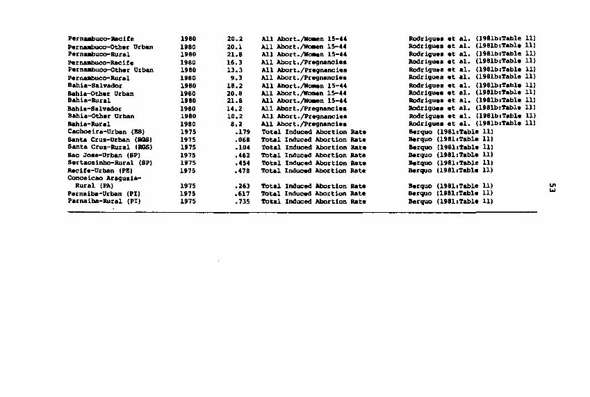
Pernaabuco-Recife 1980 20.2 All Abort.lNO-en l5-~~ Rodrique. et ale (198lblTable 11)PerlllUlbuco-Other Orban 1lI80 20.1 All Abort.;wo.en l5-~~ Rodrique. et ale (198lblTable 11)Pernambuco-Rural 1980 21.8 All Abort.lNomen l5-~~ Rodrigue. et ale (198lblTable 11)Pernaabuco-Recife 1980 16.3 All Abort./pregnaneie. Rodrique. et ale (198lblTable 11)PerlllUlbuco-other Orban 1980 13.3 All Abort./Pregnaneie. Rodrigue. et ale (198lblTable 11)Pernaabuco-Rural 1lI80 9.3 All Abort./Pregnancie. Rodrigue. et ale (198lblTable 11)Bahia-Salvador 1980 18.2 All Abort.lNomen l5-~~ Rodrigue. et ale (198lblTable 11)Bahia-other Urban 1980 20.8 All Abort.lNomen l5-~~ Rodrigue. et ale (198lblTable 11)Bahia-Rural 1lI80 21.8 All Abort.lNO-en l5-~~ Rodrigue. et ale (198lblTable 11)Bahia-Salvador 1980 14.2 All Abort./Pregnancie. Rodrique. et ale (198lblTable 11)Bahia-other Orban 1lI80 10.2 All Abort./Pregnaneie. Rodrique. et ale (198lblTable 11)Bahia-Rural 1980 8.2 All Abort./pregnancie. Rodrigue. et ale (198lblTable 11)Cachoeira-Orban (BS) 1975 .179 Total Induced Abortion Rate Berquo (198llTable 11)Santa Cruz-Orban (RGS) 1975 .068 Total Induced Abortion Rate Berquo (198llTable 11)Santa Cruz-Rural (RGS) 1975 .10~ Total Induced Abortion Rate Berquo (198llTable 11)Sao Jo.e-Orban (SP) 1975 .462 Total Induced Abortion Rate Berquo (198llTable 11)Sertaozinbo-Rural (SP) 1975 .~5~ Total Induced Abortion Rate Berquo (198llTable 11)Recife-Urban (PS) 1975 .478 Total Induced Abortion Rate Berquo (198llTable 11)Coneeicao Araguaia-

Rural (PA) 1975 .263 Total Induced Abortion Rate Berquo (198llTable 11) U'I

Parnaiba-Urban (PI) 1975 .617 Total Induced Abortion Rate Berquo (198llTable 11) w

Parnaiba-Rural (PI) 1975 .735 Total Induced Abortion Rate Berquo (198llTable 11)

54

nonmarriage. It is one thing to assume that most birthsaccrue to women in unionsJ it is quite another to assumethat all pregnancies, particularly those that are aborted,are within unions. In all likelihood, a significantfraction of abortions may be experienced by women who arenot in unions. To the extent that these abortions areunderstated, the estimate of nonmarriage may be over­stated.

For illustrative purposes, a range for the totalabortion rate of 0.5 to 1.5 per women may be assumed.With an estimated 1976 total fertility rate of 4.4,yielding about 3.75 aillion births in Brazil, a rangeestimate of between 500,000 and 1,250,000 annual inducedabortions is implied. While these figures fall well belowthe 3 aillion annual abortions derived by extrapolationfrom newspaper and other reports, they seea more plaus­ible than the very low abortion rates yielded by surveydata.

Breastfeedinq/Postpartum Amenorrhea

Statistical data on breastfeeding and postpartum amenor­rhea in Brazil are also quite deficient. Questions onbreastfeeding were included only in more recentinquiries--the NIHR and CPS. However, the data are moreconsistent for the purpose of calculating Bongaarts'index of the effect of postpartum infecundibility onfertility than was the case with abortion. Mean or medianmonths of breastfeeding are provided in reports on theNIHR and CPS by Anderson et ale (1981) and Berquo (1980),as shown in Table 14. Calculation of the Bongaarts indexrequires a transformation of mean or median months ofbreastfeeding to months of postpartum amenorrhea, whichis the -i- in the formula for the indexl Ca· 20/18.5+ i. Anderson calculated i for Bahia, Pernambuco, RioGrande do Norte, and Paraiba using the Lesthaege-Pagemodel schedules, and a formula based on this schedule wasused to transform the remaining observations.

While not representative of the entire Brazilianpopulation, the data in Table 14 do span a broad enoughspectrum of experience, from poorer Northeastern areas tothe industrialized Southeast and the more developed ruralareas of the South, to permit speculation about a plau­sible national-level index. The index values in thetable, as well as the breastfeeding data on which theyare based, show that the practice of breastfeeding is

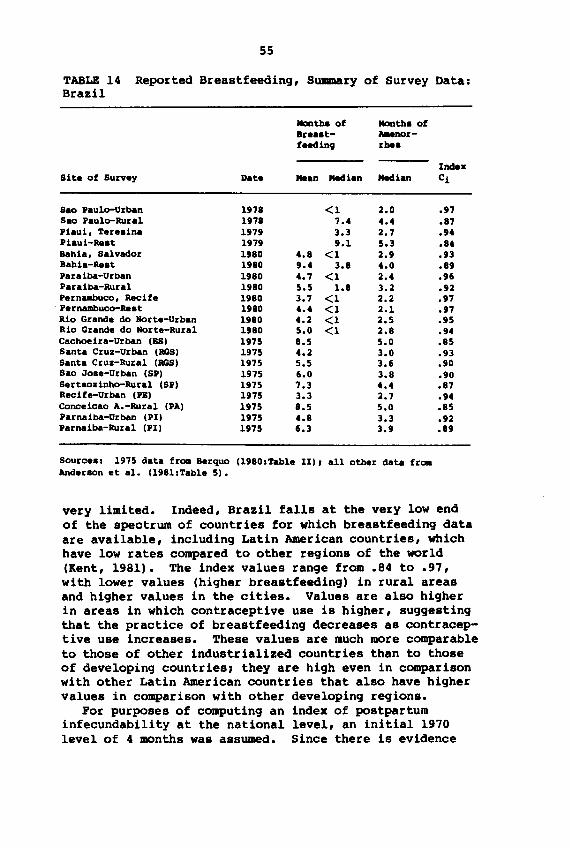
55

TABLE 14 Reported Breastfeeding, Summary of Survey Data:Brazil

IIClntha of Months ofBreast- AMnor-fHdillCJ rbea

IndexSite of Survey Date Mean Median Median Ci

Sao Paulo-Urban 1978 <1 2.0 .97Sao Paulo-Rural 1978 7.4 4.4 .87Piaui, Teresina 1979 3.3 2.7 .94Piaui-Rest 1979 9.1 5.3 .84Bahia, Salvador 1980 4.8 <1 2.9 .93Bahia-Rest 1980 9.4 3.8 4.0 .89Paraiba-Urban 1980 4.7 <1 2.4 .96Paraiba-Rural 1980 5.5 1.8 3.2 .92Pernambuco, Recife 1980 3.7 <1 2.2 .97Pernambuco-Rest 1980 4.4 <1 2.1 .97Rio Grande do Norte-Urban 1980 4.2 <1 2.5 .95Rio Grande do Norte-Rural 1980 5.0 <1 2.8 .94Cachoeira-Urban (BS) 1975 8.5 5.0 .85Santa Cruz-Urban (aGS) 1975 4.2 3.0 .93Santa Cruz-Rural (aGS) 1975 5.5 3.6 .90Sao Jose-Urban (SP) 1975 6.0 3.8 .90Sertaozinho-Rural (SP) 1975 7.3 4.4 .87Recife-Urban (PE) 1975 3.3 2.7 .94Coneeicao A.-Rural (PA) 1975 8.5 5.0 .85Parnaiba-Urban (PI) 1975 4.8 3.3 .92Parnaiba-Rural (PI) 1975 6.3 3.9 .89

Sources: 1975 data froa Berquo (1980:Table II), all other data froaAnderson et ale (198l:Table 5).

very limited. Indeed, Brazil falls at the very low endof the spectrum of countries for which breastfeeding dataare available, including Latin American countries, whichhave low rates compared to other regions of the world(Kent, 1981). The index values range from .84 to .97,with lower values (higher breastfeeding) in rural areasand higher values in the cities. Values are also higherin areas in which contraceptive use is higher, suggestingthat the practice of breastfeeding decreases as contracep­tive use increases. These values are much more comparableto those of other industrialized countries than to thoseof developing countriesJ they are high even in comparisonwith other Latin American countries that also have highervalues in comparison with other developing regions.

For purposes of computing an index of postpartuminfecundability at the national level, an initial 1970level of 4 months was assumed. Since there is evidence

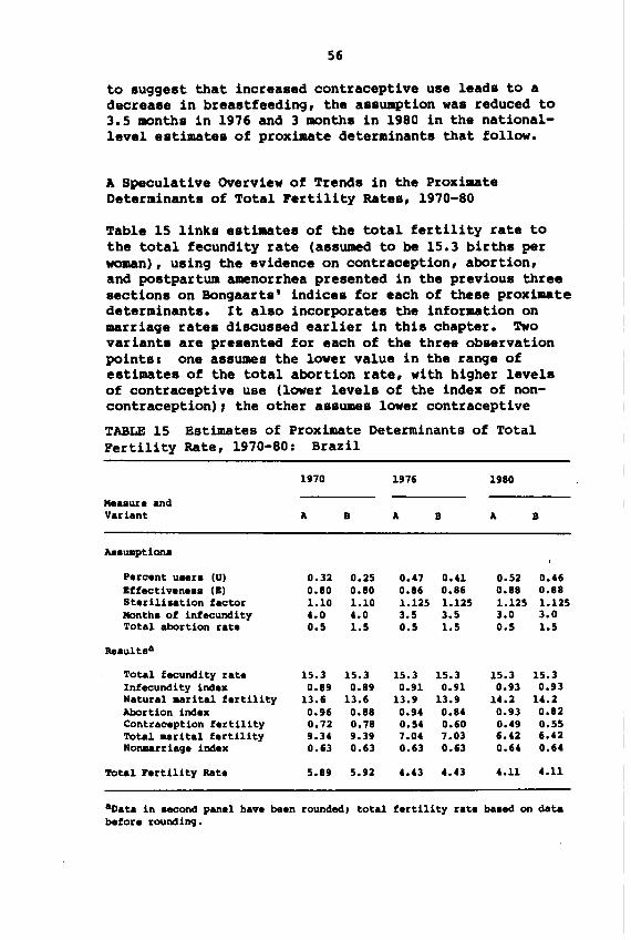
56

to suggest that increased contraceptive use leads to adecrease in breastfeeding, the assumption was reduced to3.5 months in 1976 and 3 months in 1980 in the national­level estimates of proximate determinants that follow.

A Speculative OVerview of Trends in the ProximateDeterminants of Total Pertility Rates, 1970-80

Table 15 links estimates of the total fertility rate tothe total f.cundity rate (assumed to be 15.3 births perwoman), using the evidence on contraception, abortion,and postpartum amenorrhea presented in the previous threesections on Bongaarts' indices for each of these proximatedeterminants. It also incorporates the information onmarriage rates discussed earlier in this chapter. Twovariants are presented for each of the three observationpoints I one assumes the lower value in the range ofestimates of the total abortion rate, with higher levelsof contraceptive use (lower levels of the index of non­contraception), the other assumes lower contraceptive

TABLE 15 Estimates of Proximate Determinants of TotalFertility Rate, 1970-80: Brazil

Meaaure andVariant

1970

A B

1976

A B

1980

A B

Percent uaera (U)Bffectiveneaa (B)Sterilisation factorMontha of infecundityTotal abortion rate

Reaultsa

Total fecundity rateInfecundity indexNatural aerital fertilityAbortion indexContraception fertilityTotal aerital fertilityNonaarriage index

Total Fertility Rate

0.32 0.25 0.47 O.U 0.52 0.460.80 0.80 0.86 0.86 0.88 0.881.10 1.10 1.125 1.125 1.125 1.1254.0 4.0 3.5 3.5 3.0 3.00.5 1.5 0.5 1.5 0.5 1.5

15.3 15.3 15.3 15.3 15.3 15.30.89 0.89 0.91 0.91 0.93 0.93

13.6 13.6 13.9 13.9 U.2 U.20.96 0.88 0.94 0.84 0.93 0.820.72 0.78 0.54 0.60 0.49 0.559.34 9.39 7.04 7.03 6.402 6.420.63 0.63 0.63 0.63 0.64 0.64

5.89 5.92 4.43 4.43 4.11 4.11

aData in aecond panel have been rounded, total fertility rate baaed on databefon rounding.

57

use, and the higher estimate of the total abortion rate.This is only one of several tradeoffs that a range ofvalues in the abortion rate implies. Higher abortionrates could also imply less effective contraception, aswell as a lower impact of nonmarriage to the extent thatabortions are used to terminate the pregnancies of womenoutside of unions.

The underlying assumptions are summarized in the firstpanel of the table. The contraceptive use and effective­ness rates in variant -A- are based on Table 12. Thereduction in the contraceptive use rate in variant -B- isproportional to the increase in the abortion index impliedby the higher total abortion rate. Both variants assumethat there is a decline in postpartum infecundity of about0.5 months from 1970 to 1976 that relates to increasedcontraceptive use, with a similar decline for 1976 to1980. No change is assumed between 1970 and 1976 in theindex of nonmarriage, which is consistent with theobserved trend for that period, while a small increase isshown for 1980.

In variant -A-, the main factor accounting for thedecline in the total fertility rate from its level ofaround 5.9 in 1970 to 4.4 in 1976 is the decrease inCcJ this reflects increased contraceptive use, as wellas increased effectiveness deriving from a higher propor­tion of more effective methods (the pill and steriliza­tion) among those used. To the extent that variant -A­understates the abortion rate, this conclusion should bemodified by assuming a smaller increase in contraceptiveuse, less improvement in contraceptive effectiveness, ora lower level of nonmarriage. Variant -B- illustratesthe first of these possibilities.

Extrapolating to 1980, the table suggests that thepace of the decline in total fertility could be slower inthe last half of the decade. This is partly a result ofusing levels of Cc in 1976 large enough to account forthe 1970-76 decline, combined with Cc values for 1980that are consistent with the survey results reported inTable 11. Variant -B- suggests an even slower decline inCc ' assuming that abortions played a greater role inthe decline in total fertility than is implied in variant-A.- It is worth noting that special tabulations of the1977 and 1978 PNAD survey data in fact suggest a slowingof the pace of the decline of total fertility (Leite,1981). An alternative hypothesis is that flaws in thedesign of the 1976 survey produced an overstatement ofthe decline, a point that will prove difficult to test

58

until data for making alternative estt.&tes of fertilityduring the decade become available (i.e., 1980 censusdata, for which the own-children aethad could be applied).

CONCLUSI~S

The 1970s brought a significant acceleration in thedecline of fertility in Brazils the crude birth ratefell from 41 per 1,000 in the late 1960s to 34 per 1,000in the late 1970s, the total fertility rate, a morerefined measure of fertility, declined from around 5.8births per 1,000 wo.en around 1970 to around 4.4 birthsby 1976. Of the three de-agraphic factors that couldaccount for a decline in the birth rate (proportionsmarried, age structure, and marital fertility), decliningmarital fertility was clearly responsible for the change.

Assessment of the effect of nuptiality on fertility iscomplicated by the questionable reliability of reportedmarital status in the available census and survey data.A number of factors suggest that the proportion of youngerwomen (up to age 25) reported as married has been under­stated. Doubts about the proportions married remain evenafter adjustments to include single women reporting birthsand separated women who might have entered into a secondunion and did not report it because divorce was notlegally recognized. The whole question of pregnanciesto women not in unions and the termination of such preg­nancies remains a major area of doubt in examining theproximate determinants of Brazills fertility decline.Calculations of the singulate mean age at marriage (SMAM)from census and survey data indicate a rise of about 0.8years in the mean age at marriage between 1960 and 1970,and about half that from 1970 to 1976. An alternativemeasure of the age at which wo.en begin being exposed tothe risk of childbearing, the singulate aean age at firstbirth, reveals a similar trend. Even after adjustment ofthe marital status data to account for possible under­reporting of the proportions married among women in theirearly twenties, there is little evidence of change between1970 and 1976, this suggests that changes in maritalstatus had only a limited effect on fertility declineduring that interval. Because of the demographic echo ofincreased births in the 1950. and 1960s, the age structureof the Brazilian population had a slightly positive impacton birth rates.

59

Thus, on the basis of an admittedly speculative recon­struction of -what could have happened- when Brazil'saccelerated fertility decline is decomposed into demo­graphic components and into the proximate determinants offertility, it can be concluded that a decline in maritalfertility was the primary factor responsible. Thisdecline in marital fertility can in turn be ·traced to anincreased use of effective contraception, combined withan indeterminate abortion component both within andoutside of marriage. Though national-level data on theproximate variables are lacking, survey data can be usedto construct a national-level index of noncontraception,which declined from .72-.78 in 1970 to .54-.60 in 1976and .49-.55 in 1980, suggesting that increased contracep­tion played a major role in the decline. Survey data alsoindicate a very low prevalence of breastfeeding, andsuggest a moderate attenuation of the fertility-reducingeffect of postpartum amenorrhea as contraceptionincreased. The major unknown variable is abortion. Themore one accepts the fragments of evidence that abortionis widespread in Brazil, particularly among low-incomegroups, the more one must adjust the importance attachedto increased contraception and no change in marriagerates.

Finally, it should be emphasized that doubts remainabout the reliability of data on marital status, particu­larly since a significant number of pregnancies amongwomen not in unions may be terminated by abortion, andinformal unions may be formalized only after a live birth.Census and survey data on the proportion of women inunions may therefore reflect after-the-fact social adjust­ment processes more than the exact demographic accountingneeded to decompose the proximate determinants offertility.

CHAPTER 2

SOCIOECONOMIC DIPPBREHTIALS IN FERTILITY

The evidence presented in Chapter 1 indicated that fer­tility had already declined prior to 1970 in moredeveloped regions such as the Southeast, particularlyamong higher-income groups, but not among lower-incomegroups and regions. It also suggested that the overallaccelerated decline after 1970 probably resulted from thespread of lower fertility to those latter groups. Theobjective of the present chapter is to identify thesegroups more precisely. This should make it possible tofocus an explanation of the post-1970 accelerated declinemore sharply on particular groups, and on specific socio­economic changes that may have affected their reproductivebehavior.

Evidence presented in this chapter is based on datafrom the public use sample of the 1970 census and the1976 PHAD national sample survey, both of which includequestions on average parity and on births in the yearprior to the interview. Responses were tabulated byhousehold income, education of women, rural-urban resi­dence, and region. Indirect estimating techniques wereused to derive total fertility rates for women in differ­ent education and income categories. Considerable cautionis required in interpreting the results since most of theassumptions on which the techniques are based are violatedin such an exercise. This problem is complicated by thefact that the severity of these viOlations can varybetween categories of income and education into which thepopulation has been grouped. For example, the assumptionof constant fertility would be violated to a greaterextent among higher income and education groups if theyhad been experiencing more rapid fertility decline thanlower income and education groups--the situation inBrazil in 1970. Moreover, once the population has been

60

61

divided into education and income classes, these cannotbe considered -closed- populations, another requirementfor valid application of the techniques. Sampling erroris a further problem when such divisions are made, par­ticularly for reported births in the year prior to theinterview. These biases can be reduced but not eliminatedby using fewer categories of each variable to increasesample size. In the study of fertility differences byincome category cited in Chapter 1, Carvalho and Paiva(1976) reported that such a procedure reduced the impactof interclass mobility on their estimates. This problemmay be less serious for breakdowns of the population byeducation than by income since most women, except thesmall proportion with university education, would havecompleted their education by the time they reached theirlate teens.

EDUCATION AND FERTILITY DECLINE

To examine the relation between fertility and education,women were divided into three broad education categories,with education defined according to years of schoolingcompleted: women with no schooling, those with 1-4 yearsof schooling, and those with 5 or more years. This break­down sacrifices some specificity among higher educationalgroups for a reduction in sampling error and in the mobil­ity bias mentioned above. In preliminary tabulations,the effect of education on fertility varied by rural­urban residence, suggesting that rural and urban womenshould be separated in the discussion of educational dif­ferences. To reduce the sampling error that resultedfrom having so few rural women with more than 4 years ofschooling, only two rural education classes were created:-none- and -any education.-

Computations of total fertility rates for women indifferent education groups are based on the adapted Brassmethodology described in Indirect Techniques for Demo­graphic Estimation {United Nations, 1983)J in this method,reference period error in the reporting of births duringthe year prior to the census or survey is corrected usinga factor derived from comparisons between reported parityat different ages and the parity that would accrue ifcurrent fertility were cumulated (PIP ratios). Althoughreference period error would be expected in the 1970data, which are based on a question about births in thelast year, that error should have been minimal in the

62

1976 survey, whicb recorded the date of the last birth.Estiaates prepared for the Panel on Brazil indicated anaverage PIP of 1.32 for Brazil in 1970 and 1.22 in 1976,tbis falls to 1.07 in estiaates of total fertility basedon advanced tabulations of tbe 1980 census. The 1976 PIPratios suggest tbat reference period error was stillpresent, one reason for this is that the survey was con­ducted over several weeks, and the year interval identi­fied in the tabulations aay bave excluded recent births.The Panel on Brazil elected to e~loy tbe PIP ratioadjustment in 1976, a. discu••ed further in its report.

Tbese proble.., a. well as tbe others mentioned above(interclass .ability, intercla.s differentials in recentfertility decline, and saapling error), bave undoubtedlyaffected the results reported in Table 16, whicb pre.entsestiaates of total fertility for women grouped accordingto educational attainment and rural-urban residence. Theresults are arranged in separate panels for 1970 and 1976.Tbe first row in eacb panel sbows unadjusted rates basedon reported births in tbe previous year, tbe second rowgives the average PiP ratio for women aged 20-24 and25-29. Tbe unadjusted data suggest a strong negativecorrelation between years of scbooling and total fertil­ity. Tbe question arises of wbether reference perioderror was higher among less-educated women. In 1970, thePIP ratio was 1.37 for urban women with no education andabout .10 lower for urban women with 8OI8e education. Itis doubtful that enough women in their twenties shiftedfrom the -none- class to the 1-4 group for interclassshifts to have accounted for this. On the other hand, itis possible that the PIP ratio for the 5+ group aay beexaggerated since these women had been experiencing morerapid fertility decline prior to 1970.

Although the 1976 results suggest that fertilitydecline has indeed spread to lower education groups,problems arising from PIP ratios make it very difficultto determine how much. Interclass shifting of women mayhave had a greater effect since PIP ratios dropped from1.27 in the -none- group to 1.07 in the 5+ group at thesame time that the percent of women in the -none- groupdeclined from 13.6 in 1970 to 9.5 in 1976, the 5+ cate­gory increased from 22.1 to 30.7 percent. The 1976results could also reflect higher reference period erroramong less-educated women. That survey's enumeratorswere better trained and supervised than those of thecensus, a point which suggests that reference perioderror, if present in 1976, could be related to the

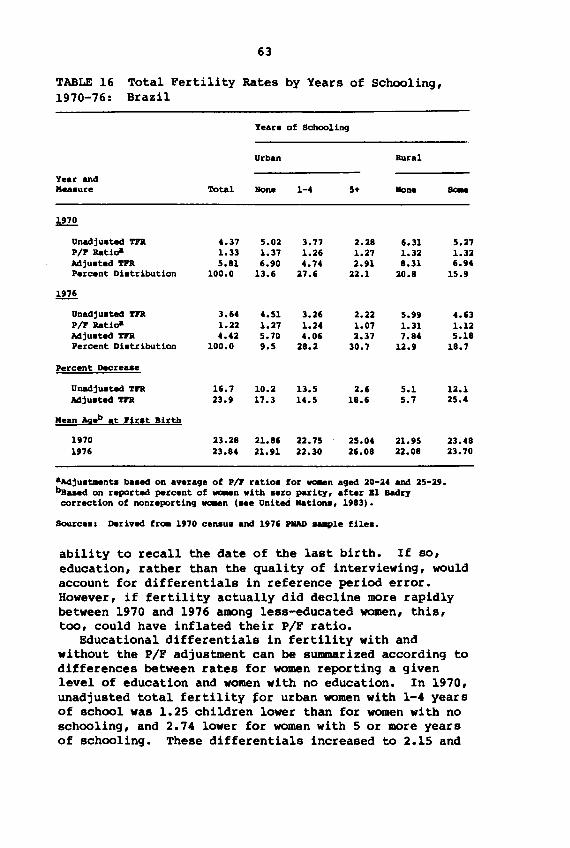
63

TABLE 16 Total Fertility Rates by Years of Schooling,1970-76: Brazil

Yeara of Schooling

Urban Rural

Year andMeaaure Total 1ione 1-4 5+ Ilone 110M

.ill.!!.

Unadjuated Tn 4.37 5.02 3.77 2.28 6.31 5.27P/F RaUaa 1.33 1.37 1.26 1.27 1.32 1.32Mjuated Tn 5.81 6.90 4.74 2.91 8.31 6.94Percent Diatribution 100.0 13.6 27.6 22.1 20.S 15.9

.!!1!Unadjuated Tn 3.64 4.51 3.U 2.22 5.99 4.63P/F RaUaa 1.22 1.27 1.24 1.07 1.31 1.12Mjuated Tn 4.42 5.70 4.06 2.37 7.84 5.1SPercent Diatribution 100.0 9.5 2S.2 30.7 12.9 18.7

Percent Deereaae

Unadjuated Tn 16.7 10.2 13.5 2.6 5.1 12.1Mjuated Tn 23.9 17.3 14.5 18.6 5.7 25.4

Mean Agab It Firat Birth

1970 23.28 21.S6 22.75 25.04 21.95 23.481976 23.84 21.91 22.30 U.08 22.08 23.70

aAdjuataenta baaed on average of P/'I ratioa for .c.en aged 20-24 and 25-29.bs...d on reported percent of .c.en with .ero parity, aftar 81 Badrycorrection of nonreporting.c.en taee United Rationa, 19S3).

Sourcea, Derived fro- 1970 cenaua and 1976 PRAD a.-ple filea.

ability to recall the date of the last birth. If so,education, rather than the quality of interviewing, wouldaccount for differentials in reference period error.However, if fertility actually did decline more rapidlybetween 1970 and 1976 among less-educated women, this,too, could have inflated their P/F ratio.

Educational differentials in fertility with andwithout the P/F adjustment can be summarized according todifferences between rates for women reporting a givenlevel of education and women with no education. In 1970,unadjusted total fertility tor urban women with 1-4 yearsof school was 1.25 children lower than for women with noschooling, and 2.74 lower for women with 5 or more yearsof schooling. These differentials increased to 2.15 and

64

3.99 children, respectively, when rates were adjustedusing observed PIP ratios. The differential betweenrural women with no education and some education was onechild when unadjusted data were used, and 1.37 childrenwith the adjustment, though rural PIP ratio. are equal,the adjustment process increases the differential betweenthe two groups because of the larger base rate for womenwith no education. In 1976, the differential betweenunadju.ted fertility rates for urban women with no educa­tion and those with 1-4 year. of schooling was again 1.25children, but decrea.ed to 2.29 children for the 5+ group.With the adjustment, the differentials were 1.64 childrenand 3.33 children, respectively. Bither way, educationaldifferentials in fertility appear to narrow among urbanwomen (when the.e differentials are expressed in numbersof children). Por rural wo.en, the opposite is true,since the 1976 differential was 1.36 with unadjusted dataand 2.66 after the adjustment (see Pigure 7).

The pattern of differentials in fertility declinebetween 1970 and 1976 is highly sensitive to PIP adjust­ments. Por urban women, the category that appears leastaffected is the 1-4 group, whose decline was about 14percent, however, its PIP ratios could have been biasedupward both by fertility decline and by population shifts.Por wo.en with no education, the decline increases from10 percent in the unadjusted rates to 17 percent afteradjustment. Por wo.en with 5+ years of schooling, thedecline increases from 3 percent to nearly 19 percent,the PIP ratio drops from 1.27 in 1970 to 1.07 in 1976 forthat group. Although the results for rural women with noeducation are not affected by the adjustment, it causesthe decline for rural wo.en with some education to double.

It is difficult to draw firm conclusions about educa­tional differentials in fertility decline from theseresults. Por urban women, unadjusted data suggest thatdeclines were greatest for wo.en with 1-4 years of school.Adjusted results suggest that declines were greater amongwomen with 5 or more years of schooling. Since there isreason to suspect that the 1970 PIP ratio for Women inthe 5+ group was biased upward by declining fertility,the 1970-76 decrease indicated by the adjusted data isprobably exaggerated. A conclusion, tentative at best,is that urban fertility decline was probably more rapidamong women with less education, leading to a narrowingof educational differentials among urban women, for ruralwomen, those with no education experienced the leastdecline, leading to a widening in these differentials.

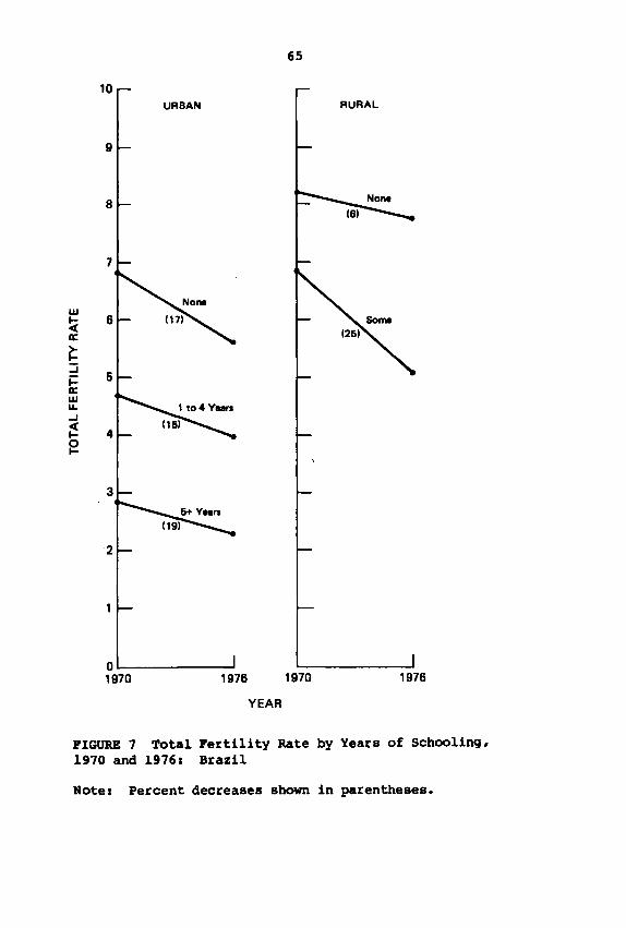
65

10URBAN

9

RURAL

8

7

w~ 6a:

~::i~a:wu....J

~~

1976

2

OL-.. ...J

1970

YEAR

1970 1976

PIGURE 7 Total Pertility Rate by Years of Schooling.1970 and 1976: Brazil

Note: Percent decreases shown in parentheses.

66

It is also i~rtant to observe that the total per­centage fertility decline between 1970 and 1976 exceededthe decline in all but one education/residence category(the adjusted rates for rural women with soge education).This is because the percentage diatribution of womena.ang education/residence categories changed between 1970and 1976. The percentage of women in the urban -none­claas declined from 13.6 percent to 9.5 percent, whilethe rural -none- dropped from 20.8 percent to 12.9percent. The shares of the urban 5+ claas increased fro.22.1 percent to 30.7 percent, while the rural -aa.e­group rose from 15.9 to 18.7 percent. The urban 1-4group was .are stable in percentage ter.., though it isi~rtant to recognize that thia stability ..aks con­siderable ahifting into and out of the group aa aconaequence of changes in the ahares of adjacent groups.Becauae of theae changes in compoaition, the averagedecline for all classes combined exceeda percentagedeclines within classes.

Insights into the relationship between education andfertility that can be extracted from tabulations ofquestions on children ever born and children born in thelast year are not limited to ea-putation of total fer­tility rates. Tabulations of first births from thesedata make it possible to measure educational differencesin the singulate mean age at first birth using the tech­nique described earlier. Theae averages are shown in thelast panel of Table 16. In 1970, there is a differenceof less than one year between urban women in the -none­category and those with 1-4 years of schooling. A muchlarger difference, 2.3 years, separates the 1-4 and 5+groups. There is a differential of about 1.5 yearsbetween rural women with no schooling and those with someschooling.

The main change in 1976 is that the average age atfirst birth for urban women in the 5+ group increases to26.1 years, while the average for women in the 1-4 groupdrops slightly, increasing the difference between thesegroups to nearly 4 years. Since the reliability of thesemeasurements could have been affected by the shifting ofwomen from one education group to the next, by decliningfertility, and by s8apling error, caution is required ininterpreting them. However, it is probably safe to saythat these differences in age at first birth are one ofthe main features of educational differentials in Brazil­ian fertility. This could be the result of later mar­riage, labor force participation, and other aspects of

67

the changing roles associated with increased education.Educational differences in the singulate .ean age atmarriage measure were not computed because of previouslymentioned doubts about the reliability of the reportingof IIarital status.

FAMILY INCC»IE

Published results of the 1976 PNAD survey included tabu­lations of fertility questions according to householdincome categories (in multiples of the .anthly salary atthe time of the survey). Berquo (1980) has ca.paredestimates of total fertility based on these tabulationsto estimates of fertility by minimum salary groups in1970 census data, with results as shown in Table 17.These estillates suggest that the greatest decline intotal fertility between 1970 and 1976 occurred a.ang thelowest-income groups. This suggests important changes inthe pattern of income-related fertility differentials inBrazil because declines prior to 1970 clearly had beenconcentrated in higher-income groups. These changes havestirred considerable interest in the question of why rapidfertility decline spread to low-income women. Before thisquestion is explored in detail in subsequent chapters, theremainder of the present chapter describes more precisely

TABLE 17 Total Fertility Rates by Family IncomeLevel (multiples of monthly minimum salary), 1970and 1976: Brazil

Total Fertility RateMonthly Incane:MUltiples of theMinimum Salary

<1<1 to <2< 2 to <5>5

1970

7.666.204.352.60

1976

6.115.944.072.54

PercentDecline

20.24.26.42.3

Source: Berquo (1980), using 1970 census and 1976PNAD survey data.

68

changes in the relationship between incoae and fertilityin Brazil.

There are several ways in which the rates reported inTable 17 are ambiguous or might have been distorted. Onerelates to the effect of changes in the composition ofwomen by income class. Again, in no group, including thelowest-income, does the decline exceed the 24 percentaverage for all groups combined, suggesting that changingcomposition haa been at work. The effects of changingcomposition by income class are acre complicated than thechanges in education deacribed above. There is an addedproblem of definition: the aeaning of miniaua salarycategoriea as indices of poverty or wealth changed overthe period from 1970 to 1976 because of deterioration inthe purchasing power of the minimum salarYJ thus fer­tility changes observed for a particular minimua salaryclass could reflect the movement of women into or out ofthe class, or changes in the way that the claas reflectsincome distribution. In 1970, 39 percent of familiesreported income levels of one minimum salary or less, and21 percent had two or more. By 1976, the share offamilies with less than one minimum salary had fallen to21 percent, while those with two or more had increased to54 percent. The extent to which these shifts representinterclass mobility rather than changes in the meaning ofminimum salary classes is ambiguous. Bither could explainwhy the largest fertility declines seem limited to thelowest minimum salary group. Nearly half of the women inthe one-two class in 1976 belonged to the less than oneclass in 1970, Which means that they could well haveexperienced a decline from 7.66 to 5.94 (22 percent), afigure that is closer to the national average.

Another ambiguity relates to the extent to which thesechanges in composition, as well as interclass differen­tials in prior fertility decline and s.-pling error, mayhave distorted P/F ratios used to adjust total fertilityrates reported in Table 17. If the tabulations by educa­tional level are a valid indication, there could be majorproblems.

A third ambiguity, also suggested by the educationresults, arises from the possible masking of quite dif­ferent rural and urban patterns in income group averagesthat combine rural and urban women.

Access to the raw data files for both the 1970 censussample and the 1976 PNAD survey make it possible toexperiment with alternative tabulations by income classaimed at reducing, or at least clarifying, these distor-

69

tions. To avoid the definitional problem arising fromcategorizing income groups according to minimum salary,families were regrouped into family income deciles (withfamilies in mUltifamily households considered as separateunits). In doing this, a choice had to be made betweentotal family income and family income per capita. Neithermeasure was entirely satisfactory& for a given level ofincome, grouping by total income understated the relativeprosperity of smaller households, whereas grouping byincome per capita led to a clustering of higher-fertilitywomen in the lower-income category. When total fertilityrates for women categorized as low-income by both defini­tions were compared to results for women with no educa­tion, the rate for the low per capita category was higher,enough so that the grouping by total family income wasselected.

In tabulating questions on fertility for differentfamily income deciles, decile categories were grouped toreduce sampling error and the impact of interclassmobility. The following groups were adopted: in urbanareas, deciles 1-3 were labeled -low,- deciles 4-6-middle,- and deciles 7-10 -high-r in rural areas, thetop two groups were combined because of sampling errorarising from the limited number of cases in the 7-10category. Interclass mobility is reduced but noteliminated by this grouping since the deciles refer tothe distribution of all families, and the composition ofgroups could change as a result of changes in thedistribution of women by place of residence or income.

Total fertility rates calculated from responses tofertility questions tabulated for groups of family incomedeciles are presented in Table 18. The format of thetable is similar to that of Table 16, which describedfertility differences by educational level: unadjustedrates in the first row, followed by observed P/F ratios,adjusted rates, and the percentage distribution of womenin 1970 and 1976. The table also shows percentagedecreases in rates from 1970 to 1976 and singulate meanages at first birth for both dates.

In the unadjusted rates for 1970, total fertility forthe urban low group was actually .4 children less thanfor the middle group. The reason that this did not showup in Table 16 is that in 1970, the majority of low-incomewomen resided in rural areas, which weighs heavily in theoverall low-income average. Unadjusted total fertilityfor urban women in the high-income class was over 2 chil­dren lower than for those in the middle class, and in

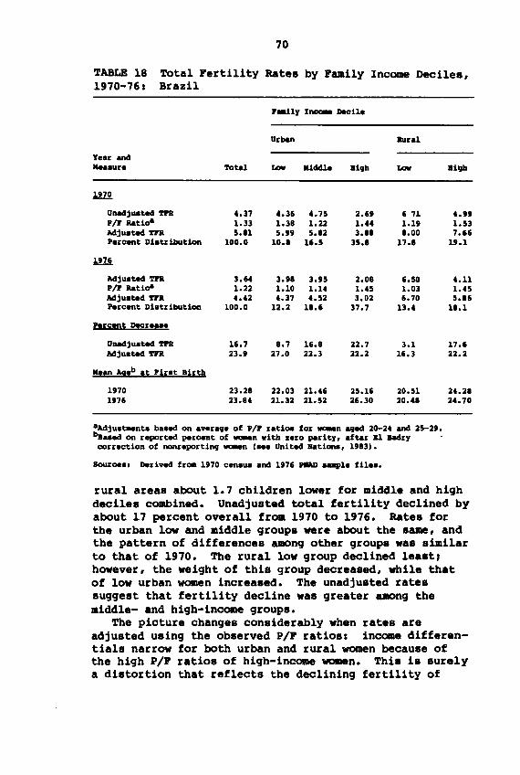
TABLE 181970-761

70

~tal Pertility Rates by Pamily Income Deciles,Brazil

F.-J.1y l~ Deeil.

Urbul lbara1

lear and.....ur. '1'ota1 Low Midd1. Bigb Low BiiJh

1m.

Qnadjuata4 T1"R 4.37 4.36 4.75 2.61 6 71 4.11P!F Ratidl 1.33 1.38 1.22 1.44 1.19 1.53lIdju.ta4 T1"R 5.11 5.99 5.12 3.11 1.00 7.66P.rc.nt Di.tribution 100.0 10.1 U.5 35.1 17.1 19.1

U76

Adju.ta4 T1"R 3.64 3. !II 3.95 2.08 6.50 4.11P!F Rati08 1.22 1.10 1.14 1.45 1.03 1.45lIdju.tad T1"R 4.42 4.37 4.52 3.02 6.70 5.16P.rcent Di.tribution 100.0 12.2 11.6 37.7 13.4 11.1

Perc.nt Deer....

Unadju.ta4 T1"R 16.7 8.7 16.8 22.7 3.1 17.6lIdju.ta4 T1"R 23.9 27.0 22.3 22.2 16.3 22.2

Mean !gab at Firat Birth

1970 23.28 22.03 21.46 25.16 20.51 24.21U76 23.84 21.32 21.52 26.30 20.41 24.70

aAdju.t:Mnt. baud on average of P!F ratioa for _n aged 20-24 and 25-29.baaaed on reported percent of wc.an with aero parity, aftar n Badry .correction of nonreporting ..-en <_ United ..tiona, UUI.

Source. I Derived frOlB 1!170 cenau. and U76 PMD ....,1. fil•••

rural areas about 1.7 children lower for middle and highdeciles combined. Unadjusted total fertility declined byabout 17 percent overall from 1970 to 1976. Rates forthe urban low and middle groups were about the same, andthe pattern of differences among other groups was similarto that of 1970. The rural low group declined lea.t,however, the weight of this group decreased, while thatof low urban women increased. The unadjusted ratessuggest that fertility decline was greater among themiddle- and high-income groups.

The picture changes considerably when rates areadjusted using the observed PIP ratiosl income differen­tials narrow for both urban and rural women because ofthe high PIP ratios of high-income women. This is surelya distortion that reflects the declining fertility of

71

women in this group. Because 1976 P/F ratios were lowerfor all women except those in the urban high-income group,the adjusted rates suggest more rapid declines than dothe unadjusted rates. The pattern of fertility declineby income class also changes, with the adjusted ratesindicating that decline to have been greatest among low­income urban women and least among low-income rural women.Though the P/F ratio of high-income women is probablydistorted, there is little change in it from 1970 to 1976,thus the percentage decline for the group is unaffected.

The insights provided by these results about incomeclass differentials in the level and percentage declineof fertility between 1970 and 1976 are thus clouded bydistortions in the P/F ratios. However, they do suggesta need to modify the conclusion reported earlier thatfertility decline was concentrated in the lowest-incomegroup and that little or no decline occurred at higherlevels. Moreover, the results indicate that if fertilitydecline was greater among low-income women, it was amonglow-income urban women, in fact, they suggest that therate of decline was lowest among low-income rural women.Otherwise, the evidence reported here indicates thatfertility decline was more evenly spread across incomeclasses. If this is so, education may have played a moreimportant role than income in differentials in the rateof decline between 1970 and 1976. There may also be aninteraction between education and income, that is, fer­tility change may be related to a woman's level of educa­tion, but the nature of this relation may vary by incomeclass.

The last bit of information about income class differ­entials in fertility relates to the measure of mean ageat first birth. The patterns here are similar to thoseobserved in the educational breakdowns, with a differ­ential of about 3 years separating high-income women fromother groups in 1970 and an increase in this differentialto about 4 years for urban women in 1976. This againraises the question of what socioeconomic forces led toincreases in age at first birth for these women and notfor women in lower income and education groups, it alsoraises the question of how differences by income andeducation relate to each other.

A partial answer to the last question is provided byan examination of joint percentage distributions of womenby educational attainment and family income level, asshown in Table 19. The base for the percentages is thetotal number of women aged 15-49, thus each cell in the

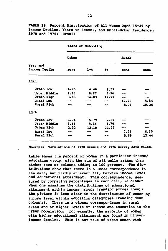
72

TABLE 19 Percent Distribution of All Women Aged 15-49 byIncome Deciles, Years in School, and Rural-Urban Residence,1910 and 1916: Brazil

Years of SChooling

Year andIncc.e Decile

Urban LowUrban MiddleUrban 8ighRural LowRural 8igh

Urban LowUrban MiddleUrban 8ighRural LowRural 8igh

Urban

Hone

4.784.933.83

3.743.462.32

1-4

4.468.27

14.83

5.799.34

13.10

5+

1.523.26

17.29

2.625.79

22.27

Rural

Hone

12.208.73

7.215.69

5.5410.36

6.2012.44

Sources: Tabulations of 1970 census and 1976 survey data files.

table shows the percent of women in a particular income/education group, with the sum of all cells rather thaneither rows or columns adding to 100 percent. The dis­tributions show that there is a loose correspondence inthe data, but hardly an exact fit, between income leveland educational attainment. This correspondence, mea­sured by comparing percentages in each cell, is closerwhen one examines the distributions of educationalattainment within income groups (reading across rows) J

the picture is less clear in the distribution of women byincome level within education categories (reading downcolumns). There is a closer correspondence in ruralareas and at higher levels of income and education in theurban population: for example, the majority of womenwith higher educational attainment are found in higher­income deciles. This is not true of urban women with

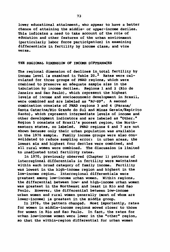
73

lower educational attainment, who appear to have a betterchance of attaining the middle- or upper-income deciles.This indicates a need to take account of the role ofeducation and other features of the urban environment(particularly labor force participation) in examiningdifferentials in fertility by income class, and viceversa.

THE REGIONAL DIMENSION OF INCOME DIFFERENCES

The regional dimension of declines in total fertility byincome level is examined in Table 20. 1 Rates were cal­culated for three groups of PNAD regions, which werecOmbined to preserve an adequate sample size in thetabulation by income deciles. Regions 1 and 2 (Rio deJaneiro and Sao Paulo), which represent the highestlevels of income and socioeconomic development in Brazil,were combined and are labeled as ·RJ-Sp·. A secondcombination consists of PNAD regions 3 and 4 (Parana/Santa Catarina/Rio Grande do Sul and Minas Gerais/BspiritoSanto), which represent intermediate levels of income andother development indicators and are labeled as ·Other.·Region 5 consists of Brazil's poorest region, the North­eastern states, so labeled. PNAD regions 6 and 7 are notshown because only their urban population was availablein the 1976 sample. Family income groups were also con­solidated to reduce sampling error: in urban areas, thelowest six and highest four deciles were combined, andall rural women were combined. The discussion is limitedto unadjusted total fertility rates.

In 1970, previously observed (Chapter 1) patterns ofinterregional differentials in fertility were maintainedwithin each broad category of family income. Fertilitywas lowest in the high-income region and highest in thelow-income region. Interregional differentials weregreatest among low-income urban women. Within regions,the differential between low- and high-income urban womenwas greatest in the Northeast and least in Rio and SaoPaulo. However, the differential between low-incomeurban women and rural women generally (most of whom arelower-income) is greatest in the middle group.

In 1976, the pattern changed. Most importantly, ratesfor women in middle-income regions moved closer to thosefor women in Rio and Sao Paulo. In fact, the rates forurban low-income women were lower in the ·other· region,so that the within-region differential for urban women

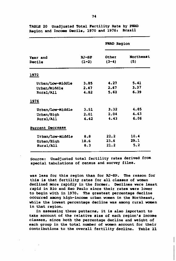
74

TABLE 20 Unadjusted Total Fertility Rate by PNADRegion and Income Decile, 1970 and 1976: Brazil

PNAD Region

Year and RJ-SP Other NortheastDecile (1-2) (3-4) (5)

1970

Urban/Low-Middle 3.85 4.27 5.41Urban/Middle 2.47 2.67 3.37Rural/All 4.82 5.62 6.39

1976

Urban/Low-Middle 3.51 3.32 4.85Urban/High 2.01 2.04 4.43Rural/All 4.42 4.43 6.06

Percent Decrease

Urban/Low-Middle 8.8 22.2 10.4Urban/High 18.6 23.6 29.1Rural/All 8.3 21.2 5.2

Source: Unadjusted total fertility rates derived fromspecial tabulations of census and survey files.

was less for this region than for RJ-SP. The reason forthis is that fertility rates for all classes of womendeclined more rapidly in the former. Declines were leastrapid in Rio and Sao Paulo since their rates were lowerto begin with in 1970. The greatest percentage declineoccurred among high-income urban women in the Northeast,while the lowest percentage decline was among rural womenin that region.

In assessing these patterns, it is also important totake account of the relative size of each region's incomeclasses, since both the percentage decline and weight ofeach group in the total number of women account for theircontributions to the overall fertility decline. Table 21

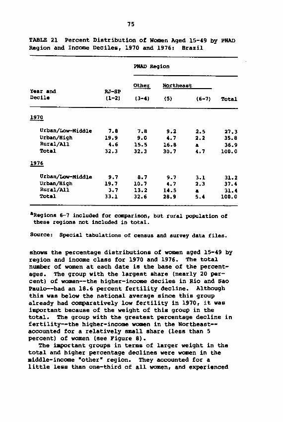
75

TABLE 21 Percent Distribution of Women Aged 15-49 by PNADRegion and Income Deciles, 1970 and 1976: Brazil

PNAD Region

~ NortheastYear and RJ-SPDecile (1-2) (3-4) (5) (6-7) Total

ill..Q.

Urban/Low-Middle 7.8 7.8 9.2 2.5 27.3Urban/8igh 19.9 9.0 4.7 2.2 35.8Rural/All 4.6 15.5 16.8 a 36.9Total 32.3 32.3 30.7 4.7 100.0

ill!

Urban/Low-Middle 9.7 8.7 9.7 3.1 31.2Urban/Bigh 19.7 10.7 4.7 2.3 37.4Rural/All 3.7 13.2 14.5 a 31.4Total 33.1 32.6 28.9 5.4 100.0

aRegions 6-7 included for comparison, but rural population ofthese regions not included in total.

Source: Special tabulations of census and survey data files.

shows the percentage distributions of women aged 15-49 byregion and income class for 1970 and 1976. The totalnumber of women at each date is the base of the percent­ages. The group with the largest share (nearly 20 per­cent) of women--the higher-income deciles in Rio and SaoPaulo--had an 18.6 percent fertility decline. Althoughthis was below the national average since this groupalready had comparatively low fertility in 1970, it wasimportant because of the weight of this group in thetotal. The group with the greatest percentage decline infertility--the higher-income women in the Northeast-­accounted for a relatively small share (less than 5percent) of women (see Figure 8).

The important groups in terms of larger weight in thetotal and higher percentage declines were women in themiddle-income ·other· region. They accounted for alittle less than one-third of all women, and experienced

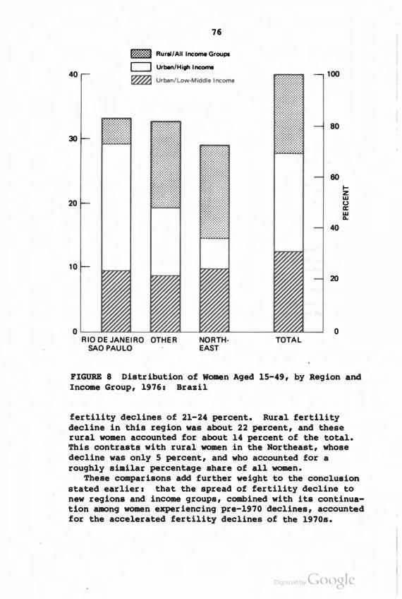
40

30

20

76

1:;:::::::::::1 Rur./AII Income GrouPi

CJ Urt.n/High IIlCOIN

~ Urban/Low-Middle Income100

80

60

40

I­ZW<.JII:W11.

10

oRIO DE JANEIRO OTHER

SAO PAULONORTH·EAST

TOTAL

20

o

FIGURE 8 Distribution of Women Aged 15-49, by Region andIncome Group, 1976. Brazil

fertility declines of 21-24 percent. Rural fertilitydecline in this region was about 22 percent, and theserural women accounted for about 14 percent of the total.This contrasts with rural women in the Northeast, whosedecline was only 5 percent, and who accounted for aroughly similar percentage share of all women.

These comparisons add further weight to the conclusionstated earlier. that the spread of fertility decline tonew regions and income groups, combined with its continua­tion among women experiencing pre-1970 declines, accountedfor the accelerated fertility declines of the 1970s.

D,qll,ZE j by CoogIe

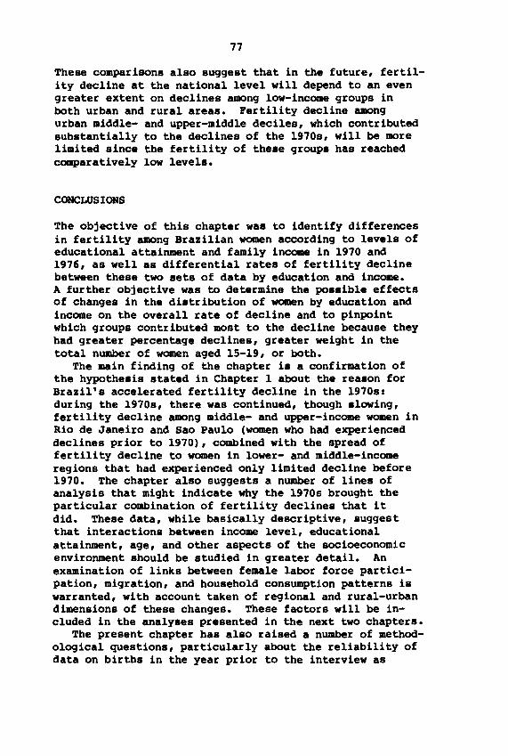
77

These comparisons also suggest that in the future, fertil­ity decline at the national level will depend to an evengreater extent on declines among low-income groups inboth urban and rural areas. Fertility decline amongurban middle- and upper-middle deciles, which contributedsUbstantially to the declines of the 1970s, will be morelimited since the fertility of these groups has reachedcomparatively low levels.

CONCLUSIONS

The objective of this chapter was to identify differencesin fertility among Brazilian women according to levels ofeducational attainment and family income in 1970 and1976, as well as differential rates of fertility declinebetween these two sets of data by education and income.A further objective was to determine the possible effectsof changes in the distribution of women by education andincome on the overall rate of decline and to pinpointwhich groups contributed most to the decline because theyhad greater percentage declines, greater weight in thetotal number of women aged 15-19, or both.

The main finding of the chapter is a confirmation ofthe hypothesis stated in Chapter 1 about the reason forBrazil's accelerated fertility decline in the 1970s1during the 1970s, there was continued, though slowing,fertility decline among middle- and upper-income women inRio de Janeiro and Sao Paulo (women who had experienceddeclines prior to 1970), combined with the spread offertility decline to women in lower- and middle-incomeregions that had experienced only limited decline before1970. The chapter also suggests a number of lines ofanalysis that might indicate why the 1970s brought theparticular combination of fertility declines that itdid. These data, while basically descriptive, suggestthat interactions between income level, educationalattainment, age, and other aspects of the socioeconomicenvironment should be studied in greater detail. Anexamination of links between female labor force partici­pation, migration, and household consumption patterns iswarranted, with account taken of regional and rural-urbandimensions of these changes. These factors will be in­cluded in the analyses presented in the next two chapters.

The present chapter has also raised a number of method­ological questions, particularly about the reliability ofdata on births in the year prior to the interview as

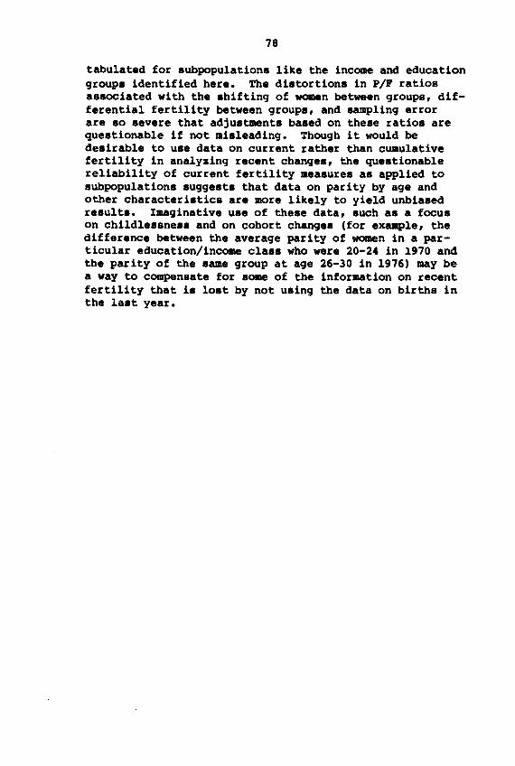
78

tabulated for subpopulations like the income and educationgroups identified here. The distortions in P/F ratiosassociated with the shifting of women between groups, dif­ferential fertility between groups, and sampling errorare so severe that adjustments based on these ratios arequestionable if not misleading. Though it would bedesirable to use data on current rather than cuaulativefertility in analyzing recent changes, the questionablereliability of current fertility measures as applied tosubpopulations suggests that data on parity by age andother characteristics are more likely to yield unbiasedresults. Imaginative use of these data, such as a focuson childlessness and on cohort changes (for example, thedifference between the average parity of women in a par­ticular education/income class who were 20-24 in 1970 andthe parity of the same group at age 26-30 in 1976) may bea way to compensate for some of the information on recentfertility that is lost by not using the data on births inthe last year.

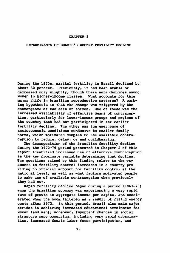
CHAPTER 3

DETERMINANTS OF BRAZIL'S RECENT FERTILITY DECLINE

During the 1970s, marital fertility in Brazil declined byabout 30 percent. Previously, it had been stable ordecreased only slightly, though there were declines amongwomen in higher-income classes. What accounts for thismajor shift in Brazilian reproductive patterns? A work­ing hypothesis is that the change was triggered by theconvergence of two sets of forces. One of these was theincreased availability of effective means of contracep­tion, particularly for lower-income groups and regions ofthe country that had not participated in the earlierfertility decline. The other was the emergence ofsocioeconomic conditions conducive to smaller familynorms, which motivated couples to use available contra­ception to reduce, delay, or end childbearing.

The decomposition of the Brazilian fertility declineduring the 1970-76 period presented in Chapter 2 of thisreport identified increased use of effective contraceptionas the key proximate variable determining that decline.The questions raised by this finding relate to the wayaccess to fertility control increased in a country pro­viding no official support for fertility control at thenational level, as well as what factors motivated peopleto make use of available contraception when previouslythey had not.

Rapid fertility decline began during a period (1967-73)when the Brazilian economy was experiencing a very rapidrate of growth in aggregate income per capita, and accel­erated when the boom faltered as a result of rising energycosts after 1973. In this period, Brazil also made majorstrides in achieving increased educational attainment forwomen (and men)J moreover, important changes in socialstructure were occurring, including very rapid urbaniza­tion, increased female labor force participation, and

79

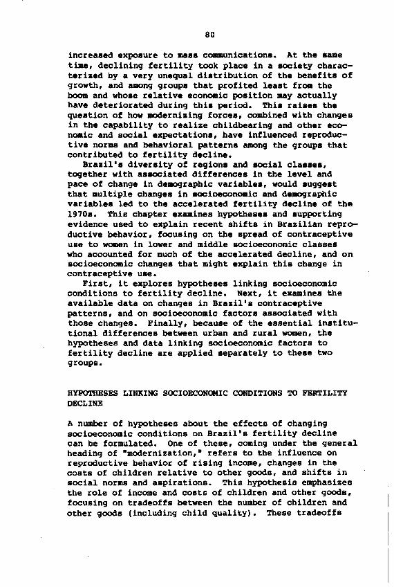
80

increa••d .xpo.ure to ma•• communication.. At the .ametime, declining fertility took plac. in a soci.ty charac­t.riz.d by a very unequal di.tribution of the ben.fit. ofgrowth, and among group. that profited l.a.t fra- theboom and who.e r.lativ••conomic po.ition may actuallyhave d.teriorated during this period. Thi. raise. thequ••tion of how .cd.rnizing forc•• , combin.d with changesin the capability to r.alize childbearing and oth.r eco­na-ic and social .xpectation., have influ.nced r.produc­tiv. norms and behavioral patt.rn. among the group. thatcontributed to fertility d.clin••

Brazil'. div.r.ity of region. and social cla•••• ,tog.th.r with a.8OCiat.d diff.r.nc•• in the l.v.l andpace of chang. in d.~raphic variabl•• , would .ugg••tthat multiple chang•• in aocioeconomic and d.~raphic

variabl•• led to the acc.lerat.d f.rtility d.clin. of the1970.. This chapter .xamines hypothes•• and .upportingevidence used to explain recent shifts in Brazilian repro­ductiv. behavior, focusing on the spr.ad of contraceptiveuse to women in lower and middle socioeconomic classeswho accounted for much of the acc.lerated decline, and onsocioeconomic change. that might .xplain this change incontraceptive u.e.

First, it explores hypothe.e. linking socioeconomicconditions to f.rtility deCline. N.xt, it examine. theavailable data on changes in Brazil's contrac.ptivepatterns, and on socioeconomic factor. associated withthose changes. Finally, becau.e of the .ssential in.titu­tional differences between urban and rural women, thehypotheses and data linking socioeconomic factors tofertility decline are applied .eparately to the.e twogroups.

HYPOTHESES LINKING SOCIOECONOMIC CONDITIONS TO FERTILITYDECLINE

A number of hypotheses about the effects of changingsocioeconomic conditions on Brazil's fertility declinecan be formulated. One of these, coming under the generalheading of -modernization,- refers to the influence onreproductive behavior of rising income, changes in thecosts of children relative to other goods, and shifts insocial norms and aspirations. This hypothesis emphasizesthe role of income and costs of children and other goods,focusing on tradeoffs between the number of children andother goods (including child quality). These tradeoffs

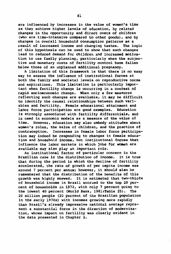
81

are influenced by increases in the value of women's timeas they achieve higher levels of education, by relatedchanges in the opportunity and direct costs of children(who are time-intensive compared to other goods), and bychanges in overall household consumption patterns as aresult of increased income and changing tastes. The logicof this hypothesis can be used to show that such changeslead to reduced demand for children and increased motiva­tion to use family planning, particularly when the sUbjec­tive and monetary costs of fertility control have fallenbelow those of an unplanned additional pregnancy.

A limitation of this framework is that there is no easyway to assess the influence of institutional forces atboth the family and societal levels on reproductive normsand aspirations. This limitation is particularly impor­tant when fertility change is occurring in a context ofrapid socioeconomic change. When only a few measuresreflecting such changes are available, it may be difficultto identify the causal relationships between such vari­ables and fertility. Female educational attainment andlabor force participation are good examples. Educationis strongly associated with fertility differentials, andis used in economic models as a measure of the value oftime. However, education may also embody attitudes aboutwomen's roles, the value of children, and the practice ofcontraception. Increases in female labor force participa­tion may indeed be responding to changes in female educa­tion and household income, but institutional forces thatinfluence the labor markets in which jobs for women areavailable may also play an important role.

An institutional factor of particular concern in theBrazilian case is the distribution of income. It is truethat during the period in which the decline of fertilityaccelerated, the rate of growth of per capita income wasaround 7 percent per annum; however, it should also beremembered that the distribution of the benefits of thisgrowth was highly skewed. It is estimated that two-thirdsof household income in Brazil accrued to the top 20 per­cent of households in 1972, with only 7 percent going tothe lowest 40 percent (World Bank, 1981:Table 25). The20 million people (20 percent of the Brazilian populationin the early 1970s) with incomes growing more rapidlythan Brazil's already impressive national average repre­sent a substantial force in the direction of moderniza­tion, whose impact on fertility was clearly evident inthe data presented in Chapter 2.

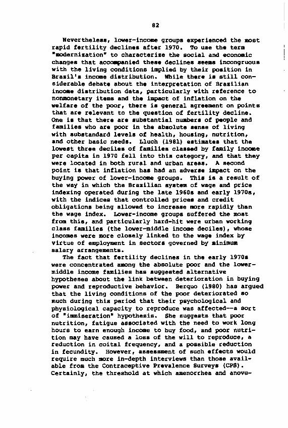
82

Nevertheless, lower-income groups experienced the mostrapid fertility declines after 1970. To use the term-modernization- to characterize the social and econoaicchanges that acca.panied these declines see.. incongruouswith the living conditions implied by their position inBrazil's income distribution. While there is still con­siderable debate about the interpretation of Brazilianincoae distribution data, particularly with reference tononmonetary items and the impact of inflation on thewelfare of the poor, there is general agreement on pointsthat are relevant to the question of fertility decline.One is that there are substantial nuabers of people andfamilies who are poor in the absolute sense of livingwith substandard levels of health, housing, nutrition,and other basic needs. Lluch (1981) estimates that thelowest three deciles of families classed by family incoaeper capita in 1970 fell into this category, and that theywere located in both rural and urban areas. A secondpoint is that inflation has had an adverse impact on thebuying power of lower-income groups. This is a result ofthe way in which the Brazilian system of wage and priceindexing operated during the late 1960s and early 1970s,with the indices that controlled prices and creditobligations being allowed to increase more rapidly thanthe wage index. Lower-income groups suffered the mostfrom this, and particularly hard-hit were urban workingclass families (the lower-middle income deciles), whoseincomes were more closely linked to the wage index byvirtue of employment in sectors governed by minimuasalary arrangements.

The fact that fertility declines in the early 1970swere concentrated among the absolute poor and the lower­middle income families has suggested alternativehypotheses about the link between deterioration in buyingpower and reproductive behavior. Berquo (1980) has arguedthat the living conditions of the poor deteriorated somuch during this period that their psychological andphysiological capacity to reproduce was affected--a SOrtof -immiseration- hypothesis. She suggests that poornutrition, fatigue associated with the need to work longhours to earn enough incoae to bUy food, and poor nutri­tion may have caused a loss of the will to reproduce, areduction in coital frequency, and a possible reductionin fecundity. However, assessment of such effects wouldrequire much more in-depth interviews than those avail­able from the Contraceptive Prevalence Surveys (CPS).Certainly, the threshold at which amenorrhea and anovu-

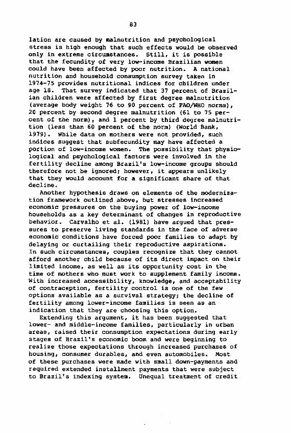
83

lation are caused by malnutrition and psychologicalstress is high enough that such effects would be observedonly in extreme circumstances. Still, it is possiblethat the fecundity of very low-income Brazilian womencould have been affected by poor nutrition. A nationalnutrition and household consumption survey taken in1974-75 provides nutritional indices for children underage 18. That survey indicated that 37 percent of Brazil­ian children were affected by first degree malnutrition(average body weight 76 to 90 percent of FAO/WHO norms),20 percent by second degree malnutrition (61 to 75 per­cent of the norm), and 1 percent by third degree malnutri­tion (less than 60 percent of the norm) (World Bank,1979). While data on mothers were not provided, suchindices suggest that sUbfecundity may have affected aportion of low-income women. The possibility that physio­logical and psychological factors were involved in thefertility decline among Brazil's low-income groups shouldtherefore not be ignored 1 however, it appears unlikelythat they would account for a significant share of thatdecline.

Another hypothesis draws on elements of the moderniza­tion framework outlined above, but stresses increasedeconomic pressures on the buying power of low-incomehouseholds as a key determinant of changes in reproductivebehavior. Carvalho et al. (1981) have argued that pres­sures to preserve living standards in the face of adverseeconomic conditions have forced poor families to adapt bydelaying or curtailing their reproductive aspirations.In such circumstances, couples recognize that they cannotafford another child because of its direct impact on theirlimited income, as well as its opportunity cost in thetime of mothers who must work to supplement family income.With increased accessibility, knowledge, and acceptabilityof contraception, fertility control is one of the fewoptions available as a survival strategy; the decline offertility among lower-income families is seen as anindication that they are choosing this option.

Extending this argument, it has been suggested thatlower- and middle-income families, particularly in urbanareas, raised their consumption expectations during earlystages of Brazil's economic boom and were beginning torealize those expectations through increased purchases ofhousing, consumer durables, and even automobiles. Mostof these purchases were made with small down-payments andrequired extended installment payments that were SUbjectto Brazil's indexing system. Unequal treatment of credit

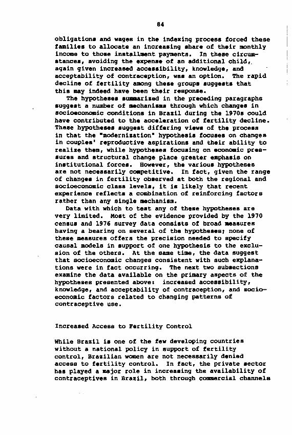
84

obligation. and wag.s in the ind.xing proc.s. forced thesefamili.. to allocat. an incr.a.ing .har. of th.ir monthlyincome to tho.e in.tallment payments. In th••e circum­.tance., avoiding the .XPen•• of an additional child,.again giv.n incr.ased acc•••ibility, knowledg., andacceptability of contrac.ption, was an option. The rapiddecline of f.rtility among th••• group••ugg••t. thatthis uy ind.ed have be.n th.ir r.spon.e.

Th. hypoth•••••~rized in the preceding paragraphs.ugg••t a number of ..chani... through which chang.. in.ocioeconomic condition. in Brazil during the 1910. couldhave contribut.d to the acc.leration of f.rtility decline.The.e hypoth•••••ugg••t diff.ring vi.w. of the proce.sin that the -mod.rnization- hypoth••i. focu.e. on changesin coupl•• ' r.productiv. aspiration. and th.ir ability torealize th.m, while hypoth••e. focu.ing on economic pres­.ur.s and .tructural chang. plac. gr.at.r .mpha.is onin.titutional force.. How.ver, the various hypothes.sare not nec•••arily competitiv.. In fact, given the rang.of chang•• in fertility ob.erved at both the regional andsocioeconomic class level., it i. lik.ly that recentexperience reflect. a combination of reinforcing factorsrather than any single ..chani.m.

Data with which to te.t any of th.se hypotheses arevery limited. Mo.t of the evidence provided by the 1910cen.u. and 1916 survey data consi.ts of broad ..a.ureshaving a bearing on several of the hypothe••sJ none ofthese measures offers the precision needed to sPecifycausal models in .upport of one hypoth.sis to the exclu­sion of the others. At the same time, the data suggestthat socioeconomic changes consistent with such explana­tions were in fact occurring. The next two sub.ectionsexamine the data available on the primary aspects of thehypotheses presented above: incr.ased acce••ibility,knowledge, and acceptability of contraception, and socio­economic factors related to changing patterns ofcontraceptive use.

Increa.ed Access to F.rtility Control

While Brazil i. one of the few developing countrieswithout a national policy in support of fertilitycontrol, Brazilian women are not necessarily d.niedaccess to f.rtility control. In fact, the private .ectorhas played a major role in increa.ing the availability ofcontraceptiv.s in Brazil, both through commercial channels

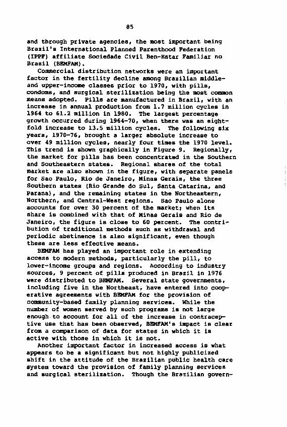
85

and through private agencies, the most important beingBrazil's International Planned Parenthood Federation(IPPF) affiliate Sociedade Civil Ben-Estar Familiar noBrasil (BEMFAM).

Commercial distribution networks were an importantfactor in the fertility decline among Brazilian middle­and upper-income classes prior to 1910, with pills,condoms, and surgical sterilization being the most commonmeans adopted. pills are manufactured in Brazil, with anincrease in annual production from 1.1 million cycles in1964 to 61.2 million in 1980. The largest percentagegrowth occurred during 1964-10, when there was an eight­fold increase to 13.5 million cycles. The following sixyears, 1910-16, brought a larger absolute increase toover 49 million cycles, nearly four times the 1910 level.This trend is shown graphically in Figure 9. Regionally,the market for pills has been concentrated in the Southernand Southeastern states. Regional shares of the totalmarket are also shown in the figure, with separate panelsfor Sao Paulo, Rio de Janeiro, Minas Gerais, the threeSouthern states (Rio Grande do Sul, Santa Catarina, andParana), and the remaining states in the Northeastern,Northern, and Central-West regions. Sao Paulo aloneaccounts for over 30 percent of the marketJ when itsshare is combined with that of Minas Gerais and Rio deJaneiro, the figure is close to 60 percent. The contri­bution of traditional methods such as withdrawal andperiodic abstinence is also significant, even thoughthese are less effective means.

BEMFAM has played an important role in extendingaccess to modern methods, particularly the pill, tolower-income groups and regions. According to industrysources, 9 percent of pills produced in Brazil in 1916were distributed to BEMFAM. Several state governments,including five in the Northeast, have entered into coop­erative agreements with BEMFAM for the provision ofcommunity-based family planning services. While thenumber of women served by such programs is not largeenough. to account for all of the increase in contracep­tive use that has been observed, BEMFAM's impact is clearfrom a comparison of data for states in which it isactive with those in which it is not.

Another important factor in increased access is whatappears to be a significant but not highly publicizedshift in the attitude of the Brazilian public health caresystem toward the provision of family planning servicesand surgical sterilization. Though the Bra~ilian govern-

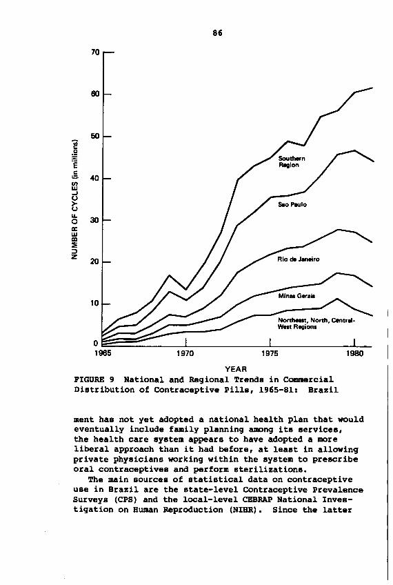
86

70

198019751970

Norm.-t, North, C8ntrel·West Regions

o~:::::::L==-~-===----l.-1965

60

10

50!.2Os

a 40(I)W...J(.)

>-(.)

u.300

a:w!Xl~::::>z

20

YEARFIGURE 9 National and Regional Trends in commercialDistribution of Contraceptive Pills, 1965-81: Brazil

ment has not yet adopted a national health plan that wouldeventually include family planning among its services,the health care system appears to have adopted a moreliberal approach than it had before, at least in allowingprivate physicians working within the system to prescribeoral contraceptives and perform sterilizations.

The main sources of statistical data on contraceptiveuse in Brazil are the state-level Contraceptive PrevalenceSurveys (CPS) and the local-level CEBRAP National Inves­tigation on Human Reproduction (NIHR). Since the latter

87

is discussed in detail in Part II, the present chapterfocuses on the CPS results. It should be noted thatbecause none of these surveys was conducted prior to1976, they provide an ex post view of the impact ofincreased access to family planning on fertility decline.Table 22 presents the percentage distributions in five ofthese surveys of married women aged 15-44 by householdincome level and contraceptive use status. The first rowof figures for each survey shows that the percentage of~omen currently using contraception increased with house­hold income, which is broken down in mUltiples of theaverage monthly minimum salary. The contraceptive usedifferential between women in upper- and lower-incomegroups was least in Sao Paulo, Brazil's most urbanizedand industrialized state, and greatest in Bahia, locatedin the lower Northeast. The remaining states shown inthe table are also located in the Northeast. Throughcooperative arrangements with state governments, BEMFAMhas operated community-based family planning programs(CBPs) in Rio Grande do Norte since 1973, followed byprograms in Pernambuco and two other Northeastern statesin 1976, and in Piaui in 1979.

Survey results for Rio Grande do Norte, the state inwhich the CBPs had been operating longest, indicate thatthe differential between higher- and lower-income womenwas less than that in Piaui and Bahia, states in whichsuch programs did not exist prior to the survey. As forcontraceptive methods, a higher proportion of women inupper-income groups had been sterilized, particularly inthe NortheastJ pills were more important relative to othermethods among lower-income women. This is especiallyevident in Rio Grande do Norte, where pill users accountedfor 43 percent of women currently contracepting in thelow-income group, and 25 percent of high-income contra­ceptors. Sterilization, in contrast, accounted for 22percent of low-income current users and 47 percent ofhigh-income users. Other methods, mainly rhythm andwithdrawal, were also important among low-income currentusersJ these methods, along with condoms, were importantas well among low-income women in the state of Sao Paulo.

When educational attainment is substituted for incomeas the measure of socioeconomic differences in contra­ceptive use, the results are virtually identical, atleast for the four states with available tabulations onwhich to base a comparison. Table 23 shows the percentageof currently married women aged 15-44 using contraceptionfor four education categories, ranging from none to some

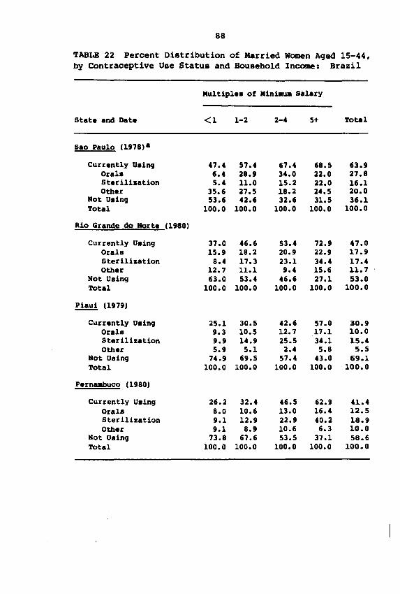
88

TABLE 22 Percent Distribution of Married women Aged 15-44,by Contraceptive Use Status and Household Income: Brazil

Multiple. of Mint.ua Salary

State and Date <1 1-2 2-4 5+ Total

Sao Paulo (1978)a

Currently O.ing 47.4 57.4 67.4 68.5 63.9Orab 6.4 28.9 34.0 22.0 27.8Stuilhation 5.4 11.0 15.2 22.0 16.1Other 35.6 27.5 18.2 24.5 20.0

Not Uaing 53.6 42.6 32.6 31.5 36.1Total 100.0 100.0 100.0 100.0 100.0

Rio Grande do Norte (1980)

Currently U.ing 37.0 46.6 53.4 72.9 47.0Orals 15.9 18.2 20.9 22.9 17.9Sterilhation 8.4 17.3 23.1 34.4 17.4Other 12.7 11.1 9.4 15.6 11.7

Not Osing 63.0 53.4 46.6 27.1 53.0Total 100.0 100.0 100.0 100.0 100.0

Piaui (1979)

Currently Oaing 25.1 30.5 42.6 57.0 30.9Orals 9.3 10.5 12.7 17.1 10.0Sterilization 9.9 14.9 25.5 34.1 15.4Other 5.9 5.1 2.4 5.8 5.5

Not Using 74.9 69.5 57.4 43.0 69.1Total 100.0 100.0 100.0 100.0 100.0

Pernaabuco (1980)

Currently O.ing 26.2 32.4 46.5 62.9 41.4Orals 8.0 10.6 13.0 16.4 12.5Sterilization 9.1 12.9 22.9 40.2 18.9Other 9.1 8.9 10.6 6.3 10.0

Not Using 73.8 67.6 53.5 37.1 58.6Total 100.0 100.0 100.0 100.0 100.0

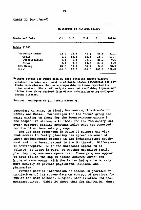
89

TABLE 22 (continued)

MUltiples of Minimum Salary

State and Date <1 1-2 2-4 5+ Total

Bahia (1980)

Currently Using 18.7 28.4 42.8 65.9 31.1Orals 6.9 13.5 15.3 15.7 11.7Sterilization 7.1 7.4 13.2 26.3 9.6Other 5.7 7.5 14.3 23.8 9.8

Not Using 81.3 71.6 57.2 34.1 68.9Total 100.0 100.0 100.0 100.0 100.0

aSource breaks Sao Paulo data by more detailed income classes.Weighted averages were used to collapse income categories for SaoPaulo into classes that were comparable to those reported forother states. Since cell weights were not available, figures maydiffer from those derived from direct tabulation using collapsedincome classes.

Source: Rodrigues et ale (198la:Table 7).

secondary or more, in Piaui, Pernambuco, Rio Grande doNorte, and Bahia. Percentages for the -none- group arequite similar to those for the lowest-income groups inthe respective states, with those for the -secondary andover- category falling somewhat below what was observedfor the 5+ minimum salary group.

The CPS data presented in Table 22 support the viewthat access to family planning has spread to women oflower socioeconomic classes in the industrialized South­east and to a lesser extent in the Northeast. Differencesin contraceptive use in the Northeast appear to berelated, at least in part, to whether organized familyplanning programs were operative. These programs appearto have filled the gap in access between lower- andhigher-income women, with the latter being able to relymore heavily on private physicians, clinics, andpharmacies.

Further partial information on access is provided bytabulations of CPS survey data on sources of services fortwo of the main methods, surgical sterilization and oralcontraceptives. Table 24 shows that for Sao Paulo, where

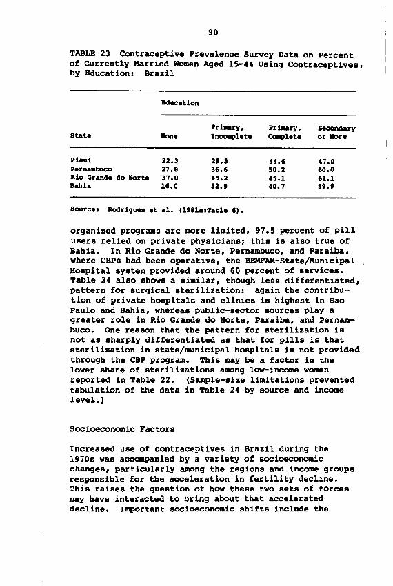
90

TABLE 23 Contraceptive Prevalence Survey Data on Percentof Currently Married women Aged 15-44 Using Contraceptives,by Education: Brazil

Bducation

State

PiauiPerlUUlbucoRio Grande do NorteBahia

None

22.327.837.016.0

Priaary,IncClllP1ete

2'.336.645.232.'

Priaary,CoIIplete

44.650.245.140.7

Sec:ondaryor More

47.060.061.15'.'

Source I Rodrigue. et a1. (l'81alTable 6).

organized programs are more limited, 97.5 percent of pillusers relied on private physiciansr this is also true ofBahia. In Rio Grande do Norte, Pernambuco, and Paraiba,where CBPs had been operative, the BEMFAM-State/MunicipalHospital system provided around 60 percent of services.Table 24 also shows a similar, though less differentiated,pattern for surgical sterilization: again the contribu­tion of private hospitals and clinics is highest in SaoPaulo and Bahia, whereas pUblic-sector sources play agreater role in Rio Grande do Norte, Paraiba, and Pernam­buco. One reason that the pattern for sterilization isnot as sharply differentiated as that for pills is thatsterilization in state/municipal hospitals is not providedthrough the CBP program. This may be a factor in thelower share of sterilizations among low-income womenreported in Table 22. (Sample-size limitations preventedtabulation of the data in Table 24 by source and incomelevel. )

Socioeconomic Factors

Increased use of contraceptives in Brazil during the1970s was accompanied by a variety of socioeconomicchanges, particularly among the regions and income groupsresponsible for the acceleration in fertility decline.This raises the question of how these two sets of forcesmay have interacted to bring about that accelerateddecline. Important socioeconomic shifts include the

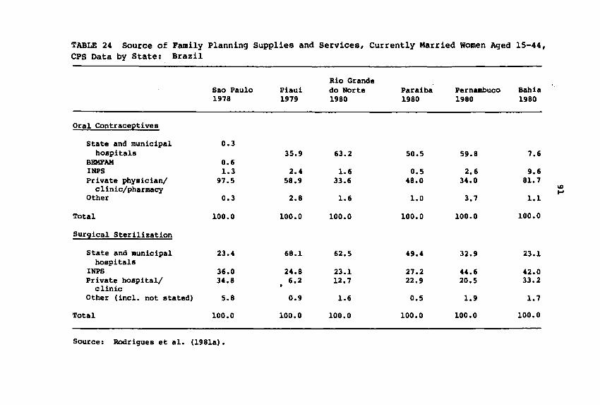
TABLE 24 Source of Family Planning Supplies and Services, Currently Married Women Aged 15-44,CPS Data by State: Brazil

Rio GrandeSao Paulo Piaui do Norte Paraiba Pernambuco Bahia1978 1979 1980 1980 1980 1980

Oral Contraceptives

State and municipal 0.3hospitals 35.9 63.2 50.5 59.8 7.6

BEMFAM 0.6INPS 1.3 2.4 1.6 0.5 2.6 9.6Private physician/ 97.5 58.9 33.6 48.0 34.0 81.7

clinic/pharmacy ID....Other 0.3 2.8 1.6 1.0 3.7 1.1

Total 100.0 100.0 100.0 100.0 100.0 100.0

Surjical Sterilization

State and municipal 23.4 68.1 62.5 49.4 32.9 23.1hospitals

INPS 36.0 24.8 23.1 27.2 44.6 42.0Private hospital/ 34.8 6.2 12.7 22.9 20.5 33.2

clinicOther (incl. not stated) 5.8 0.9 1.6 0.5 1.9 1.7

Total 100.0 100.0 100.0 100.0 100.0 100.0

Source: Rodrigues et al. (1981a).

92

changing status of women, as reflected in their educa­tional attainment and labor force participation, as wellas changes in household incoae and consumption patterns,such as the diffusion of cons~r durables like televisionreceivers, refrigerators, and gas stoves among lower­incoae group.. The.e change. could have reduced thedesire to have .are children and increased .ativation tou.e the mean. of fertility control that were becoaing.are available.

Data pre.ented in Chapter 2 on differences in thelevel and percentage of fertility decline by year. ofschooling revealed .ignificant increa.es in the educa­tional attainment of women during the 1910.. The dataalso revealed a clo.e, though not exact, corre.pondencebetween the di.tribution of woaen by educational attain­ment and household incoae decile. (Table 19). In examin­ing socioeconomic changes, the present chapter does notrepeat that breakdown by income deciles. Moreover, sucha breakdown is not used in the pre.ent discussion of therelation.hip between education and labor force participa­tion. To do so would introduce a circularity arisingfrom the contribution of woaen'. earnings to the incomeof their households I it would create the mi.leadingimpression that the proportion of women who work ishigher among household. in higher-income deciles, when infact one of the reason. that such hou.eholds fall intothose higher deciles is because the.e women work. Therelevant income variable is hou.ehold income withoutthese women's contributions. At this point, the discus­sion focuses on changes in educational attainment andtheir relationship to difference. in labor force par­ticipation.

Table 25 suggests that increases in female educationalattainment were greater in the 1910s than in the 1960s.The table shows the proportion reporting no schoolingamong women aged 20-49 by five-year age groups, in 1960,1910, 1916, and 1980. For women in their twenties, theproportion with no schooling was around 40 percent in1960, declining to about 33 percent in 1910, and to below20 percent by 1916. Increased female school enrollmentduring the 1960s accounts for part of this increaseddecline in the proportion with no schooling. Anotherfactor is various types of adult education programs,including adult literacy classes and special coursesleading to certification of equivalency at various gradelevels. Many employers in the formal sector require suchcertification, even for semiskilled labor, and these

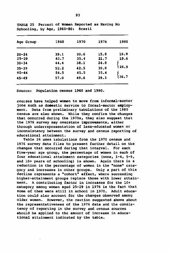
93

TABLE 25 Percent of Women Reported as Having NoSchooling, by Age, 1960-80: Brazil

Age Group 1960 1970 1976 1980

20-24 39.1 30.6 15.8 16.925-29 42.7 35.4 21.7 19.630-34 44.4 38.1 24.8

{ 26.935-39 52.2 42.5 30.840-44 54.5 45.5 35.4

{36.745-49 57.0 49.8 39.3

Source: Population census 1960 and 1980.

courses have helped women to move from informal-sectorjobs such as domestic service to formal-sector employ­ment. Data from preliminary tabulations of the 1980census are also shown. While they confirm the changesthat occurred during the 1970s, they also suggest thatthe 1976 survey may overstate improvements, eitherthrough under representation of less-educated women orinconsistency between the survey and census reporting ofeducational attainment.

Table 26 uses tabulations from the 1970 census and1976 survey data files to present further detail on thechanges that occurred during that interval. For eachfive-year age group, the percentage of women in each offour educational attainment categories (none, 1-4, 5-9,and 10+ years of schooling) is shown. Again there is areduction in the percentage of women in the -none- cate­gory and increases in other groups. Only a part of thisdecline represents a -cohort- effect, where succeedinghigher-attainment groups replace those with lower attain­ment. A contributing factor in increases for the 10+category among women aged 25-29 in 1976 is the fact thatsome of them were still in school in 1970. Adult educa­tion could also account for the changes observed amongolder women. However, the caution suggested above aboutthe representativeness of the 1976 data and the consis­tency of reporting in the survey and census sourcesshould be applied to the amount of increase in educa­tional attainment indicated by the table.

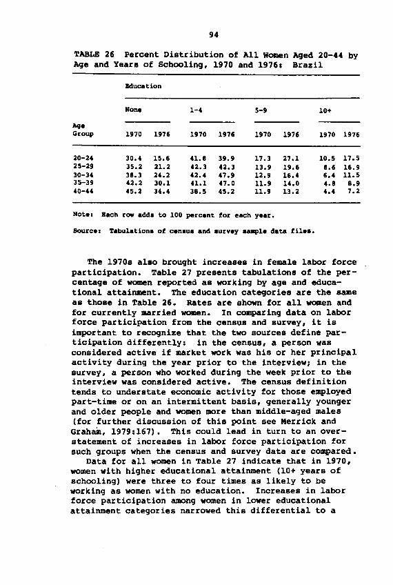
94

TABLE 26 Percent Distribution of All Women Aged 20-44 byAge and Years of Schooling, 1910 and 1916: Brazil

Bducation

None 1-4 5-9 10+

AAjeGroup 1970 1976 1970 1976 1970 1976 1970 1976

20-24 30.4 15.6 41.8 39.9 17.3 27.1 10.5 17.525-29 35.2 21.2 42.3 42.3 13.9 19.6 8.6 16.930-34 38.3 24.2 42.4 47.9 12.9 16.4 6.4 11.535-39 42.2 30.1 41.1 47.0 11.9 14.0 4.8 8.940-44 45.2 34.4 38.5 45.2 11.9 13.2 4.4 7.2

Note I Each row add. to 100 percent for each year.

Source I Tabulation. of cen.u. and .urvey • .-p1e data file••

The 1910s also brought increases in female labor forceparticipation. Table 21 presents tabulations of the per­centage of women reported as working by age and educa­tional attainment. The education categories are the sameas those in Table 26. Rates are shown for all women andfor currently married women. In comparing data on laborforce participation from the census and survey, it isimportant to recognize that the two sources define par­ticipation differently: in the census, a person wasconsidered active if market work was his or her principalactivity during the year prior to the interview7 in thesurvey, a person who worked during the week prior to theinterview was considered active. The census definitiontends to understate economic activity for those employedpart-time or on an intermittent basis, generally youngerand older people and women more than middle-aged males(for further discussion of this point see Merrick and

Graham, 1919:161). This could lead in turn to an over-statement of increases in labor force participation forsuch groups when the census and survey data are compared.

Data for all women in Table 21 indicate that in 1910,women with higher educational attainment (10+ years ofschooling) were three to four times as likely to beworking as women with no education. Increases in laborforce participation among women in lower educationalattainment categories narrowed this differential to a

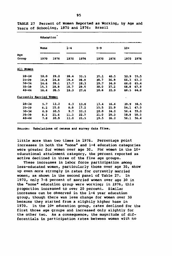
95

TABLE 27 Percent of Women Reported as Working, by Age andYears of Schooling, 1970 and 1976: Brazil

Education

None 1-4 5-9 10+

AgeGroup 1970 1976 1970 1976 1970 1976 1970 1976

All Women

20-24 18.0 29.2 26.4 35.5 35.1 40.5 52.9 55.525-29 14.8 24.8 19.4 28.9 30.7 36.9 66.3 63.330-34 14.6 28.1 17.7 28.3 29.7 34.9 66.0 65.435-39 15.3 28.9 18.7 29.5 30.0 37.2 66.8 67.840-44 16.4 28.5 18.3 27.6 28.6 33.9 66.5 64.8

Currently Married Women

20-24 5.7 12.2 6.3 13.0 13.4 16.6 39.9 38.525-29 6.2 15.0 8.0 17.2 15.5 21.9 54.1 47.530-34 6.9 20.5 9.7 20.2 18.0 24.0 56.4 55.035-39 8.2 21.6 11.3 22.7 21.0 29.3 58.9 59.540-44 7.8 20.9 11.0 21.5 19.5 26.2 56.1 56.4

Source: Tabulations of census and .urvey data file••

little more than two times in 1976. Percentage pointincreases in both the -none- and 1-4 education categorieswere greater for women over age 30. For women in the 10+educational attainment category, the percent reported asactive declined in three of the five age groups.

These increases in labor force participation amongless-educated women, particularly those over age 30, showup even more strongly in rates for currently marriedwomen, as shown in the second panel of Table 27. In1970, only 7-8 percent of married women over age 30 inthe -none- education group were working~ in 1976, thisproportion increased to over 20 percent. Similarincreases can be observed in the 1-4 year educationgroup, though there was less change for women over 30because they started from a slightly higher base in1970. In the 10+ education group, rates declined for thefirst three age groups and increased only slightly forthe other two. As a consequence, the magnitude of dif­ferentials in participation rates between women with no

96

education and those with 10+ years of schooling decreasedfrom 7 or 8 to 1-2 or 3-1.

Increased educational attainment, higher labor forceparticipation among more-educated women, and the narrow­ing of differentials in participation between .cre- andless-educated women between 1970 and 1976 combined todouble the proportion (from 15 percent to 30 percent) ofwomen who were working during the six-year period understudy. Although caution i. required because of possibleupward bia. in the 1976 data resulting fro. definitionaldifference••entioned above, the data suggest that impor­tant changes in women's roles were occurring. Increasesin labor force participation, as.ociated with increasesin the proportion of women with higher levels of educa­tion, suggest an improvement in these women's statusr onthe other hand, these trend. among women in the lowereducation classes may mean that more women were workingout of economic neces.ity.

SOCIOECONCIUC FACTORS AND FERTILITY DECLUIE AMONG URBANAND RURAL WCllEN

While the hypotheses about relationships between socio­economic factors (modernization, increased econo.icpressures on families) and fertility decline in Braziloutlined above are broadly applicable to both urban andrural woaen, differences in institutional factors suggestthat these groups be examined separately. For example,increased ownership of televisions, while not exclusivelyan urban phenomenon, is much more pronounced in urbanareas. Likewise, the influence of land availability andincreased proletarianization of farm labor is probablymore direct in rural areas. While indirect effects couldreach urban areas via migration, they are much more diffi­cult to capture with the census and PNAD survey datafiles. Based on separate samples for urban and ruralwomen extracted from these files, the next two subsectionspresent a more detailed examination of the characteristicsof currently married urban and rural women, and how thesecharacteristics relate to differentials in average parity_The focus in both SUbsections is restricted to currentlymarried women because the analysis of proximate determi­nants of fertility presented in Chapter 1 identifieddeclining marital fertility as the main component of therecent decline in Brazilian birth rates.

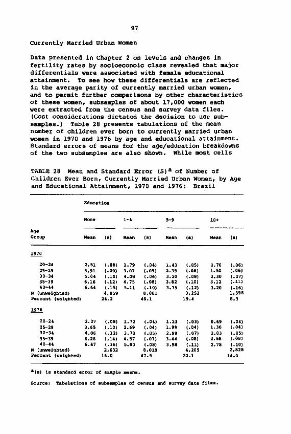
97

Currently Married Urban Women

Data presented in Chapter 2 on levels and changes infertility rates by socioeconoic class revealed that majordifferentials were associated with female educationalattainment. To see how these differentials are reflectedin the average parity of currently married urban women,and to permit further comparisons by other characteristicsof these women, sUbsamples of about 17,000 women eachwere extracted from the census and survey data files.(Cost considerations dictated the decision to use sub­samples.) Table 28 presents tabulations of the meannumber of children ever born to currently married urbanwomen in 1970 and 1976 by age and educational attainment.Standard errors of means for the age/education breakdownsof the two subsamples are also shown. While most cells

TABLE 28 Mean and Standard Error (S)a of Number ofChildren Ever Born, Currently Married Urban Women, by Ageand Educational Attainment, 1970 and 1976: Brazil

Education

AgeGroup

None

Mean (B)

1-4

Mean (B)

5-9

Mean (a)

10+

Mean (a)

1970

20-2425-2930-3435-3940-44

N (unweighted)Percent (weighted)

20-2425-2930-3435-3940-44

N (unveighted)Percent (weighted)

2.513.915.046.166.64

2.073.654.866.266.47

(.08)(.09)(.10)(.12)(.15)4,059

24.2

(.08)(.10)(.12)(.14)(.16)2,632

16.0

1.793.074.084.755.11

1.722.693.704.575.00

(.04)(.05)(.06)(.08)(.10)8,081

48.1

(.04)(.04)(.05)(.07)(.08)8,019

47.9

1.432.393.203.823.75

1.231.992.993.443.58

(.05)(.06)(.08)(.10)(.12)3,252

19.4

(.03)(.04)(.07)(.08)(.11)4,205

22.1

0.701.502.303.123.20

0.691.302.032.682.78

(.06)(.06)(.07)(.11)(.16)1,3968.3

(.04)(.04)(.05)(.08)(.10)2,828

14.0

alB) iB Btandard error of Ba.ple ..anB.

Source, TabulationB of aubBampleB of cenBua and aurvey data fi1eB.

98

are large enough at this level to minimize aampling error,further breakdowns could be affected, particularly when asmall percentage of women fall into a given category.Further tests of the significance of educational andother differences in the number of children ever born arepresented in the next chapter uaing mUltiple regression.

The basic pattern of educational differences in theaean number of children ever born is similar in 1970 and19761 comparing women in the age 40-44 category, themean number of children ever born in 1970 drops from 6.6children for women with no education to 3.2 children forthose with 10+ years of schoolingJ in 1976, the figuresare 6.5 children for women with no education and 2.8 forthose with 10+ years of schooling. The earlier averageage at marriage of women with no education is a majorfactor in differences among younger women, who had 2.5births in 1970 compared to 0.7 for the 10+ group, and 2.1compared to the 10+ group's 0.7 in 1976. The values forolder women with 10+ years of school are a problem in thatthe average of 2.8 for women aged 40-44 in 1976 is~than the 3.1 reported for those aged 35-39 in 1970.Sampling error is the most likely culprit, since the .95confidence intervals of the standard errors of the twomeans intersect. Shifts of women from the 5-9 class in1970 to the 10+ class in 1976 could not account for thissince they would bias the 1976 figure upward rather thandownward.

How do other characteristics such as work status andmigrant status affect fertility differentials? Thegeneralizations in the previous section about increasesin educational attainment and labor force participationhold for currently married urban women. From 1970 to1976, the proportion of urban women reporting no educationdeclined from 24.2 percent to 16.0 percent, while that ofwomen with 10+ years of schooling increased from 8.3 to14.0 percent. Patterns of labor force participation bylevel of educational attainment are similar to those shownin Table 27, though the differences between educationcategories are less. The top panel of Table 29 presentsparticipation rates for urban women. Part of the largedifferential between more- and less-educated women inTable 27 resulted from the lower educational attainmentand labor force participation of rural women. For urbanwomen, the order of magnitude of differences between thetop and bottom education categories was four to five,narrowing to a range of three to four in 1976. Largerproportional increases among less-educated women over age

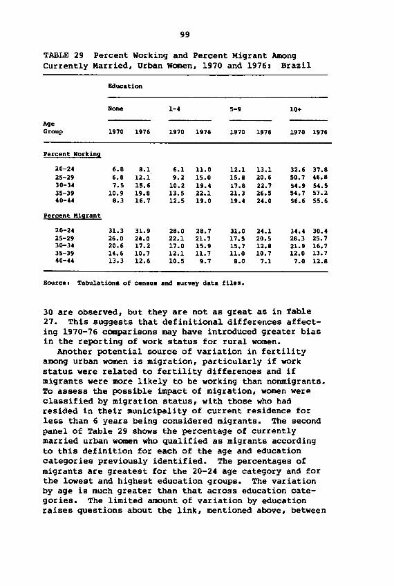
99

TABLE 29 Percent working and Percent Migrant AmongCurrently Married, Urban Women, 1970 and 1976: Brazil

Education

None 1-4 5-9 10+

AgeGroup 1970 1976 1970 1976 1970 1976 1970 1976

Percent Working

20-24 6.8 8.1 6.1 11.0 12.1 13.1 32.6 37.825-29 6.8 12.1 9.2 15.0 15.8 20.6 50.7 46.830-34 7.5 15.6 10.2 19.4 17.8 22.7 54.9 54.535-39 10.9 19.8 13.5 22.1 21.3 26.5 54.7 57.240-44 8.3 16.7 12.5 19.0 19.4 24.0 56.6 55.6

Percent Migrant

20-24 31.3 31.9 28.0 28.7 31.0 24.1 34.4 30.425-29 26.0 24.0 22.1 21.7 17.5 20.5 28.3 25.730-34 20.6 17.2 17.0 15.9 15.7 12.8 21.9 16.735-39 14.6 10.7 12.1 11.7 11.0 10.7 12.0 13.740-44 13.3 12.6 10.5 9.7 8.0 7.1 7.0 12.8

Source. Tabulations of census and survey data files.

30 are observed, but they are not as great as in Table27. This suggests that definitional differences affect­ing 1970-76 comparisons may have introduced greater biasin the reporting of work status for rural women.

Another potential source of variation in fertilityamong urban women is migration, particularly if workstatus were related to fertility differences and ifmigrants were more likely to be working than nonmigrants.To assess the possible impact of migration, women wereclassified by migration status, with those who hadresided in their municipality of current residence forless than 6 years being considered migrants. The secondpanel of Table 29 shows the percentage of currentlymarried urban women who qualified as migrants accordingto this definition for each of the age and educationcategories previously identified. The percentages ofmigrants are greatest for the 20-24 age category and forthe lowest and highest education groups. The variationby age is much greater than that across education cate­gories. The limited amount of variation by educationraises questions about the link, mentioned above, between

100

migrant statu., work .tatu., and fertility. Tabulations(not shown) of the percentage of currently married womenreported as working by age and migration status revealedno differences between migrants and nonmigrants. Thissuggests that motive. for migration other than work--.astprobably marriage--account for the variation in the pro­portion of migrant. shown in the table.

Returning to the question of increases in female laborforce participation and educational attainment, the ques­tion of whether these increases indicate changes inwomen's socioeconomic status can be further clarified byexamining the kind. of jobs involved in the increasedproportions reporting employment. For this purpose, theoccupations of employed women were grouped into four broadstatus categories: (1) high-status service occupations,including managerial, technical, and professional posi­tions, as well as higher-status jobs in the commercialand financial sectors, (2) low-status .ervice occupations,including domestic and personal services, as well as low­status commercial jobs, counter attendants, waitresses,and clerks, (3) occupations in manufacturing, and (4)others, consisting of nonmanagerial public-sector jobs,any primary-sector jobs held by urban women, and poorlydefined occupations.

Table 30 presents the percentage distributions ofcurrently married urban women according to these statuscategories and their educational attainment. The statusdistributions also include the proportion of women notworking (columns sum to 100 percent), indicating whichstatus categories absorbed employment increases in eacheducational group between 1970 and 1976. Education canbe seen to determine the kinds of jobs women hold: ofthe 8.2 percent of women in the -none- education categorywho were working in 1970, 6.8 percentage points (83 per­cent of workers) were in the low-status service and othercategories, of the 50.8 percent working among women inthe 10+ education category, 49.3 percentage points (97percent of workers) were in the high-status servicecategories. Increases in labor force participation amongless-educated women consisted mainly of more jobs in thesame category as their 1970 employment. The participationrate of women with no education increased by 6.8 percent­age points between 1970 and 1976, with low-status serviceand other occupations accounting for 90 percent of jobsheld by this group. Lower status-jobs also accounted formost of the increases in employment in the middle twoeducation classes, though manufacturing also contributed

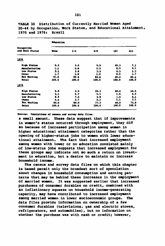
101

TABLE 30 Distribution of Currently Married women Aged20-44 by OCcupation, WOrk Status, and Educational Attainment,1970 and 1976: Brazil

OocupIltiOllaD4 Work Statu 1-4 5-, 10+ All

.1gb Statu~ectw:1Dg

Law StatuOtbeEIlot WorklDg~tal

Ugh Statullanuf~w:1Dg

Law Statu.otIo.E!lot WorklDg~tal

0.3 2.0 ,., 41.3 7.11.1 2.1 2.2 0.3 2.15.1 3.1 3.2 0.3 3.71.7 1.1 1.' 0.' 1.7

11.1 II.' 12.1 41.2 15.4100.0 100.0 100.0 100.0 100.0

0.1 2.5 10.3 41.4 10.52.3 5.7 5.3 1.0 4.41.5 7.2 4.1 1.' '.14.4 3.7 2.3 1.1 3.1

14.0 10.' 77.3 46.' 75.'100.0 100.0 100.0 100.0 100.0

SouECltI. 'rabuletiODe of _. aD4 !IlU'NY data f11•••

a sllllll a~unt. These data suggest that if illprovuaentsin wc.en I s status occurred through ellplopaent, they didso because of increased participation .-eng wa.en inhigher educational attainaent categories rather than theopening of higher-status jobs to wc.en with lower educa­tional attainment. The fact that increased ellplo~nt

a~ng wc.en with lower or no education consisted aainlyof low-status jobs suggests that increased ellplo~nt forthese groups lilly indicate not so .uch a return on invest­_nt in education, but a desire to lIllintain or increasehousehold incc.e.

The census and survey data files on which this chapteris based per.it only the broadest sort of speculationabout changes in household consuaption and earning pat­terns that lilly be behind these increases in the ellplo~nt

of IIllrried wc.en. It was suggested earlier that increasedpurchases of consu.er durables on credit, combined withan inflationary squeeze on household inco.e-generatingcapacity, lilly have contributed to increased ellplo~nt

a~ng IIllrried wc.en in lower soc:ioeconaaic groups. Thedata files provide inforJllltion on ownership of a fewconsu.er durables (televisions, gas and electric stoves,refrigerators, and auta.obiles), but no information onwhether the purchase was with cash or credit, however,

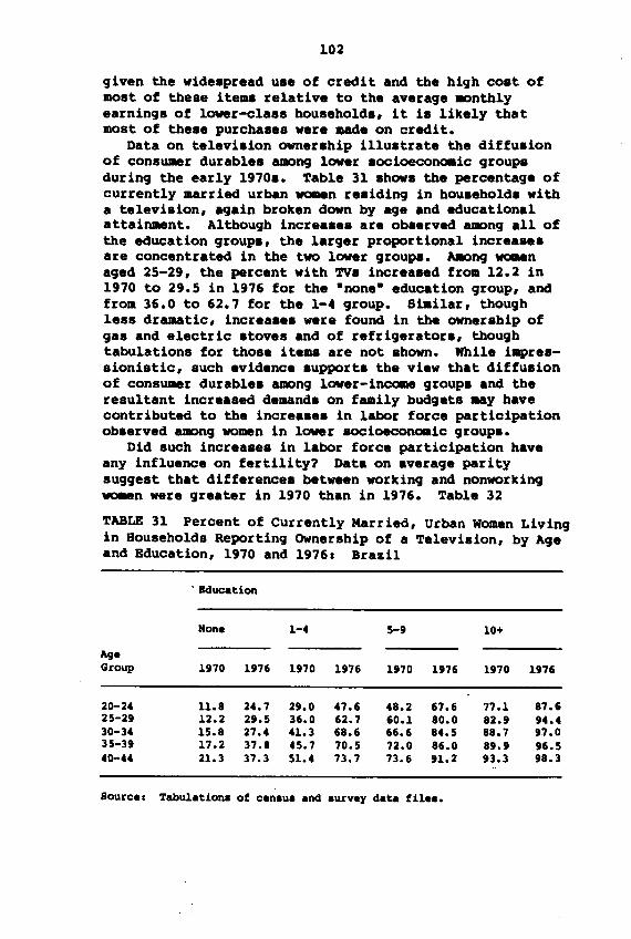
102

given the wide.pread u.e of credit and the high co.t ofmost of these items relative to the av.rag• .anthlyearnings of lower-class hous.hold., it i. lik.ly thatmost of th••• purcha••s w.r. aad. on credit.

Data on t.l.vi.ion own.r.hip illu.trat. the diffu.ionof consumer durabl•• among low.r .ocioeconaaic group.during the early 1970.. Tabl. 31 .how. the perc.ntag. ofcurrently married urban women r ••iding in hou••hold. witha t.levision, .g.in brok.n down by age .nd education.lattainment. Although incre•••• are ob••rved among .11 ofthe education group., the l.rger proportional incr.a...are conc.ntr.t.d in the two low.r group.. A.ang womenag.d 25-29, the perc.nt with TV. incr.a••d from 12.2 in1970 to 29.5 in 1976 for the -non.- .duc.tion group, andfrom 36.0 to 62.7 for the 1-4 group. at-ilar, thoughl.ss dramatic, incr.a.e. w.re found in the owner.hip ofgas and electric .tov.s .nd of r.frig.rator., thoughtabulations for those items are not .hown. Whil. illpr••­sionistic, such .vid.nc••upport. the vi.w th.t diffu.ionof consumer durabl.. among low.r-income group. .nd theresultant incr••sed d.mand. on family budg.ts ..y h.vecontribut.d to the incre•••• in labor fore. participationob.erved among women in lower aocioeconaaic group••

Did such incr.a.e. in l.bor fore. participation h.v.any influ.nc. on fertility? Dat. on .v.rage paritysuggest th.t diff.rence. betwe.n working and nonworking~n were gr••ter in 1970 th.n in 1976. Tabl. 32

TABLE 31 Percent of Curr.ntly Marri.d, Urban Nom.n Livingin Households Reporting Own.rship of a T.levision, by Ag.and Bducation, 1970 and 19761 Brazil

. Bducation

None 1-4 5-11 10+

AgeGroup l!I70 l!I76 l!I70 l!I76 1!170 11176 11170 l!I76

20-24 11.8 24.7 211.0 47.6 48.2 67.6 77.1 87.625-211 12.2 211.5 36.0 62.7 60.1 80.0 82.11 114.430-34 15.8 27.4 41.3 68.6 66.6 84.5 88.7 !I7.035-311 17.2 37.8 45.7 70.5 72.0 86.0 811.11 116.540-44 21.3 37.3 51.4 73.7 73.6 1Il.2 113.3 118.3

Source. Tabulation. of cen.u. and .urvey data file••

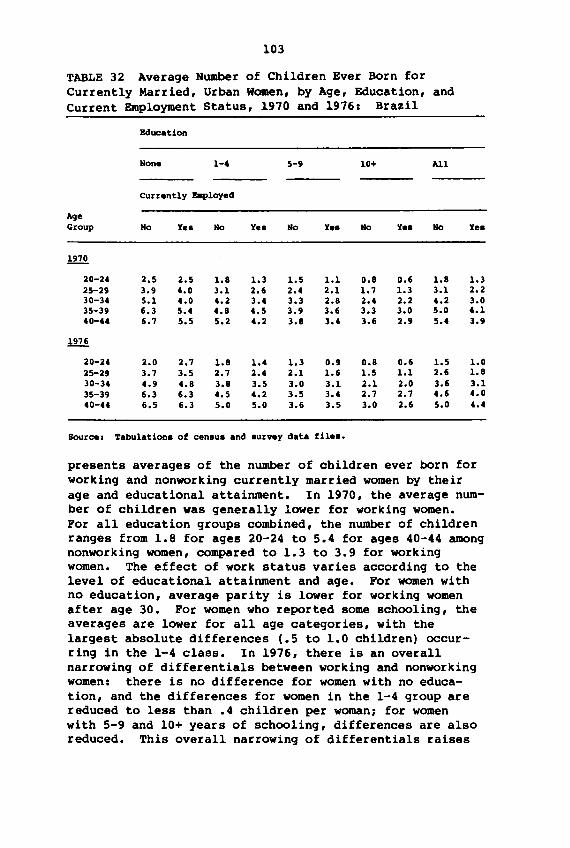
103

TABLE 32 Average Number of Children Ever Born forCurrently Married, Urban Women, by Age, Education, andCurrent Employment Status, 1970 and 1976: Brazil

Education

lIone 1-4 5-9 10+ All

Currently Bap10yed

AgeGroup No Yes No Yes No No Yes Yes

.!ru!.

20-2425-2930-3435-3940-44

1976

20-2425-2930-3435-3940-44

2.5 2.5 1.8 1.3 1.5 1.1 0.8 0.6 1.8 1.33.9 4.0 3.1 2.6 2.4 2.1 1.7 1.3 3.1 2.25.1 4.0 4.2 3.4 3.3 2.8 2.4 2.2 4.2 3.06.3 5.4 4.8 4.5 3.9 3.6 3.3 3.0 5.0 4.16.7 5.5 5.2 4.2 3.8 3.4 3.6 2.9 5.4 3.9

2.0 2.7 1.8 1.4 1.3 0.9 0.8 0.6 1.5 1.03.7 3.5 2.7 2.4 2.1 1.6 1.5 1.1 2.6 1.84.9 4.8 3.8 3.5 3.0 3.1 2.1 2.0 3.6 3.16.3 6.3 4.5 4.2 3.5 3.4 2.7 2.7 4.6 4.06.5 6.3 5.0 5.0 3.6 3.5 3.0 2.6 5.0 4.4

Source. Tabulations of census and survey data files.

presents averages of the number of children ever born forworking and nonworking currently married women by theirage and educational attainment. In 1970, the average num­ber of children was generally lower for working women.For all education groups combined, the number of childrenranges from 1.8 for ages 20-24 to 5.4 for ages 40-44 amongnonworking women, compared to 1.3 to 3.9 for workingwomen. The effect of work status varies according to thelevel of educational attainment and age. For women withno education, average parity is lower for working womenafter age 30. For women who reported some schooling, theaverages are lower for all age categories, with thelargest absolute differences (.5 to 1.0 children) occur­ring in the 1-4 class. In 1976, there is an overallnarrowing of differentials between working and nonworkingwomen: there is no difference for women with no educa­tion, and the differences for women in the 1-4 group arereduced to less than .4 children per woman~ for womenwith 5-9 and 10+ years of schooling, differences are alsoreduced. This overall narrowing of differentials raises

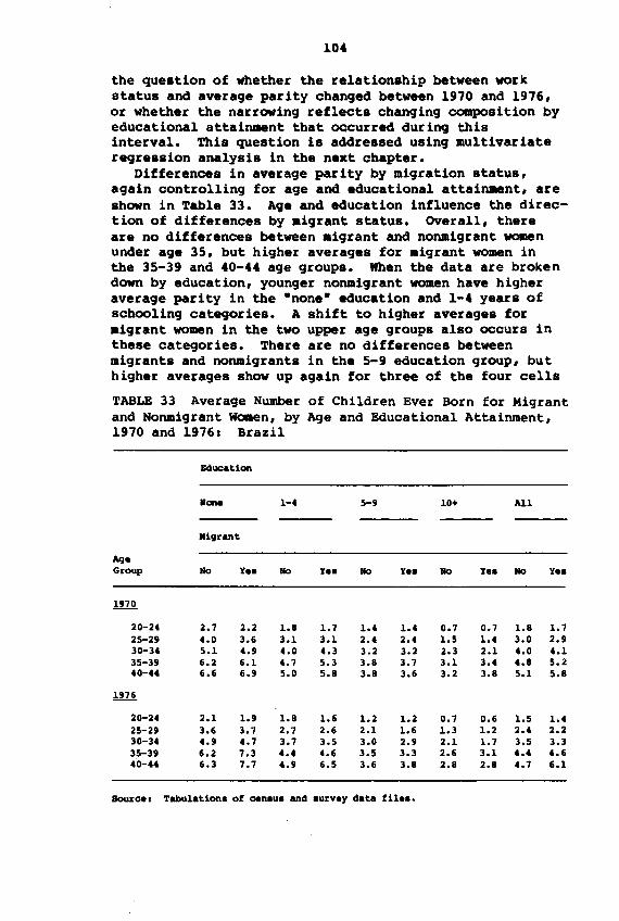
104

the question of whether the relationship between workstatus and average parity changed between 1970 and 1976,or whether the narrowing reflects changing composition byeducational attainment that occurred during thisinterval. This question is addressed using multivariateregression analysis in the next chapter.

Differences in average parity by migration status,again controlling for age and educational attainment, areshown in Table 33. Age and education influence the direc­tion of differences by aigrant status. Overall, thereare no differences between aigrant and nonmigrant womenunder age 35, but higher averages for aigrant women inthe 35-39 and 40-44 age groups. When the data are brokendown by education, younger nonmigrant women have higheraverage parity in the -none- education and 1-4 years ofschooling categories. A shift to higher averages foraigrant women in the two upper age groups also occurs inthese categories. There are no differences betweenmigrants and nonmigrants in the 5-9 education group, buthigher averages show up again for three of the four cells

TABLE 33 Average Number of Children Ever Born for Migrantand Nonmigrant WODen, by Age and Educational Attainment,1970 and 1976: Brazil

Education

Mone 1-4 5-9 10+ All

Migrant

Ag.Group Ilo Y.a Ilo Y.a Ilo Y.a Ilo Yea Ilo Y.a

1970

20-24 2.7 2.2 1.8 1.7 1.4 1.4 0.7 0.7 1.8 1.725-29 4.0 3.6 3.1 3.1 2.4 2.4 1.5 1.4 3.0 2.930-34 5.1 4.9 4.0 4.3 3.2 3.2 2.3 2.1 4.0 4.135-39 6.2 6.1 4.7 5.3 3.8 3.7 3.1 3.4 4.8 5.240-44 6.6 6.9 5.0 5.8 3.8 3.6 3.2 3.8 5.1 5.8

1976

20-24 2.1 1.9 1.8 1.6 1.2 1.2 0.7 0.6 1.5 1.425-29 3.6 3.7 2.7 2.6 2.1 1.6 1.3 1.2 2.4 2.230-34 4.9 4.7 3.7 3.5 3.0 2.9 2.1 1.7 3.5 3.335-39 6.2 7.3 4.4 4.6 3.5 3.3 2.6 3.1 4.4 4.640-44 6.3 7.7 4.9 6.5 3.6 3.8 2.8 2.8 4.7 6.1

Source a Tabulationa of a.naua and aurv.y data fi1.a.

105

containing older migrant women in the 10+ education cate­gory. The higher average parity among older migrant womenprobably reflects the fact that these women made recentmoves as members of a family unit, whereas a large shareof the moves of recent younger migrants may have beenassociated with or occurred before marriagei this couldexplain why nonmigrants with lower educational attainmenthad higher average parity.

The data on links between selected measures of thesocioeconomic status of currently married urban women anddifferentials in their average parity raise several issuesfor further analysis. After controlling for age, thegreatest differentials in average parity are those asso­ciated with educational attainment, with significantlylower levels of average parity being observed among womenwith higher levels of education. Since there were impor­tant shifts of women to higher education categoriesbetween 1970 and 1976, increased education stands out asa key factor among the socioeconomic variables associatedwith fertility declines during that interval. However,the question remains of whether the impact of educationwas mainly a change in the distribution of women byeducational attainment, or whether and how education mayhave interacted with other variables, perhaps with changesin its relationship to fertility differentials resultingfrom changes in those variables. For example, averageparity was lower among working than nonworking women, butthe nature of this relationship was conditioned by educa­tion. Work status itself was closely associated witheducational attainment, with a greater proportion ofworking women among those with higher education. However,increases in the percentage of women working between 1970and 1976 were greatest for those in lower educationalcategories. One effect of this was a narrowing of thedifferential in average parity between working and non­working women between 1970 and 1976. This suggests thatsomething beyond changes in educational composition mayhave been at work, perhaps along the lines of the argumentsuggested earlier about increased work to maintain house­hold income or to finance increased consumption of con­sumer durables. Though the census and survey files pro­vide little supporting evidence for this idea, the dataon increased ownership of televisions among less-educatedwomen support such a view. Although the links betweenmigrant status and differences in average parity are lessclear, those that do appear were conditioned by educationand age.

106

Currently Married Rural Women

For currently married rural women, differences in averageparity may reflect not only variation in individual andhousehold characteristics, but also institutional factorssuch as availability of and access to land, land tenure,and differences in modes of agricultural production.Again, Brazil's regional diversity is important. Tradi­tionally, high rural fertility in Brazil suggests thatchildren have been an important asset to rural familiesJresearch on subsistence farmers in the Northeast hasrevealed that even very young children contribute tohousehold production (Almeida, 1977).

A number of hypotheses have been suggested about theeffects of recent socioeconomic changes in Brazil on ruralfertility differences. One is that increased scarcity ofland in more settled areas has reduced the value of chil­dren as farm laborers and made it more difficult for chil­dren to acquire a farm through inheritance. Researchbased on data from the 1970 population and agriculturalcensuses indicated that fertility was lower in moresettled regions of Southeastern Brazil and higher on theagricultural frontier. However, the link between fer­tility and land availability was also conditioned byinstitutional factors, particularly Brazil's unequaldistribution of land (Merrick, 1978)J rural fertility inNortheastern Brazil was much less responsive to landscarcity as a consequence (Merrick, 1981).

Paiva (1982) has argued that the proletarianization ofrural labor (the shift of farm labor out of smallholderstatus into wage labor as a result of the consolidationof land into larger holdings) has contributed to Brazil'srecent fertility decline. He suggests that the effectsof proletarianization in Brazil differ from the Europeanexperience described by Tilly (1978) and others, wherefertility increased because the formation of new farmfamilies was linked to having a plot of land.

These hypotheses will be discussed further in Chapter4. The remainder of the present chapter explores differ­ences in the average parity of currently married ruralwomen in Brazil, using cross-tabulations that control forage and other socioeconomic variables. Subsamples forrural women were extracted from the 1970 census and 1976survey data files. Since the 1976 survey did not includerural areas in the Northern and Central-Western regionsof Brazil, the data on rural women are restricted to theNortheastern, Southeastern, and Southern states. Regional

107

breakdowns follow the grouping adopted in Chapter 2, withthe first consisting of the Northeast, the second includ­ing the states of Rio de Janeiro and Sao Paulo (labeledRJ-SP), and the remaining states (Minas Gerais, EspiritoSanto, Parana, Santa Catarina, and Rio Grande do Sul)constituting a third group labeled ·other.· In Chapter2, unadjusted total fertility rates for rural areas ofthese three groups of states showed that while fertilitywas lowest in Rio and Sao Paulo in 1970, fertility declinebetween 1970 and 1976 was most rapid in the ·other· group,which fell between RJ-SP and the Northeast in level ofsocioeconomic development.

The same pattern appears when average parity is brokendown by region, with controls for age and education.Table 34 presents data on the mean number of childrenever born for currently married rural women in the threeregional groups, with women grouped according to whetherthey had no education or reported any years of schoolingcompleted. Average parity in 1970 was uniformly higherin the Northeast, with no apparent difference betweenthose with none and those with some education. In 1970,the latter category accounted for only 26 percent ofwomen in the region, this proportion increased to 39percent in 1976, at which time differences by educationalattainment also became observable. For example, therewas only 0.1 difference for women aged 25-29 in 1970, buta .8 difference in 1976. In the other two regions, halfof the women reported having some education in 1970, withthe proportion rising to 65 percent in RJ-SP and 67 per­cent in the ·other· group in 1976. In 1970, averageparity was lower for rural women with some education inboth regions, and this differential widened in 1976: forwomen aged 25-29, the differential was .4 in 1970 for the·other· group, increasing to 1.0 in 1976, for RJ-SP, itincreased from .8 to 1.0. This indicates a more rapidfertility decline in the former region, which is con­sistent with the findings reported in Chapter 2.

To what extent does variation in other socioeconomiccharacteristics of rural women relate to differences inaverage parity? Table 35 presents the percentages ofcurrently married rural women according to three charac­teristics, two of these (work status and migration status)were also examined for urban women, while the third (pro­letarianization) was defined to explore the hypothesisthat shifts of the rural population into wage labor con­tributed to recent fertility declines. To measure prole­tarianization, women were grouped according to whether

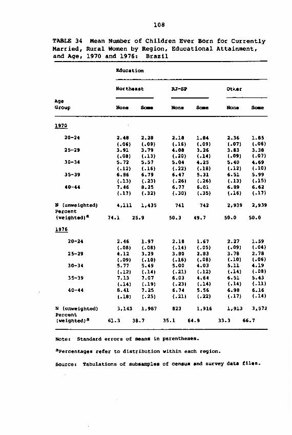
108

TABLE 34 Mean Number of Children Ever Born for CurrentlyMarried, Rural Women by Region, Educational Attainment,and Age, 1970 and 1976: Brazil

Education

Northeast RJ-SP Ot•.er

AgeGroup None SolIe None SOBle None SOlIe

ill.2.20-24 2.48 2.28 2.18 1.84 2.36 1.85

(.06) (.011) (.16) ( .0111 ( .07) (.06)25-211 3. !Il 3.711 4.08 3.26 3.83 3.38

(.081 (.13) (.20) (.141 ( .011) ( .07)30-34 5.72 5.57 5.04 4.25 5.40 4.611

(.12) (.161 ( .22) ( .18) (.12) (.10135-311 6.86 6.711 6.47 5.31 6.51 5.1111

(.13) (.23) (.261 ( .26) (.13) ( .15140-44 7.46 8.25 6.77 6.01 6.811 6.62

(.171 ( .32) (.30) (.35) ( .16) (.17)

N (unweighted) 4,111 1,435 741 742 2,11311 2,11311Percent(weightedl a 74.1 25.11 50.3 411.7 50.0 50.0

11176

20-24 2.46 1.117 2.18 1.67 2.27 1.511(.081 (.08) (.141 ( .05) (.0111 (.04)

25-211 4.12 3.211 3.80 2.83 3.78 2.78(.0111 (.10) (.16) (.08) (.10) (.06)

30-34 5.77 5.411 5.00 4.03 5.11 4.111(.121 (.141 (.21) (.12) (.14) (.081

35-311 7.13 7.07 6.03 4.64 6.51 5.43(.14) ( .l!I) ( .231 (.14) (.14) (.11)

40-44 8.41 7.25 6.74 5.56 6.118 6.16(.181 (.25) (.211 (.22) (.17) (.14)

N (unweighted) 3,143 1,1187 823 1,!Il6 1,!Il3 3,572Percent(weighted) a 61.3 38.7 35.1 64.11 33.3 66.7

Note I Standard errors of means in parentheses.

apercentages refer to distribution within each region.

Source I Tabulations of subsamp1es of census and survey data files.

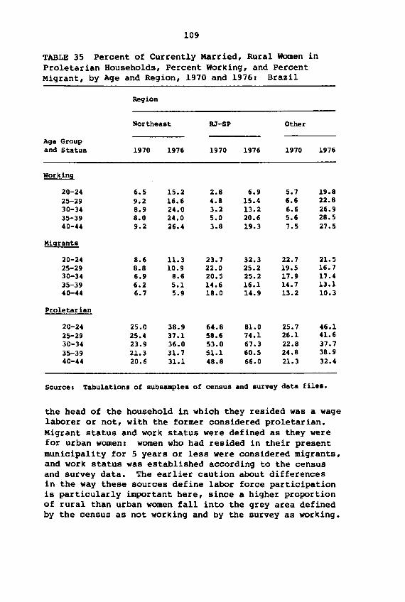
109

TABLE 35 Percent of Currently Married, Rural Women inProletarian Households, Percent Working, and PercentMigrant, by Age and Region, 1970 and 1976: Brazil

Region

Northeast RJ-SP Other

Age Groupand Status 1970 1976 1970 1976 1970 1976

Working

20-24 6.5 15.2 2.8 6.9 5.7 19.825-29 9.2 16.6 4.8 15.4 6.6 22.830-34 8.9 24.0 3.2 13.2 6.6 26.935-39 8.0 24.0 5.0 20.6 5.6 28.540-44 9.2 26.4 3.8 19.3 7.5 27.5

Migrants

20-24 8.6 11.3 23.7 32.3 22.7 21.525-29 8.8 10.9 22.0 25.2 19.5 16.730-34 6.9 8.6 20.5 25.2 17.9 17.435-39 6.2 5.1 14.6 16.1 14.7 13.140-44 6.7 5.9 18.0 14.9 13.2 10.3

Proletarian

20-24 25.0 38.9 64.8 81.0 25.7 46.125-29 25.4 37.1 58.6 74.1 26.1 41.630-34 23.9 36.0 53.0 67.3 22.8 37.735-39 21.3 31.7 51.1 60.5 24.8 38.940-44 20.6 31.1 48.8 66.0 21.3 32.4

SOurce I Tabulations of subsamp1e. of census and survey data file••

the head of the household in which they resided was a wagelaborer or not, with the former considered proletarian.Migrant status and work status were defined as they werefor urban women: women who had resided in their presentmunicipality for 5 years or less were considered migrants,and work status was established according to the censusand survey data. The earlier caution about differencesin the way these sources define labor force participationis particularly important here, since a higher proportionof rural than urban women fall into the grey area definedby the census as not working and by the survey as working.

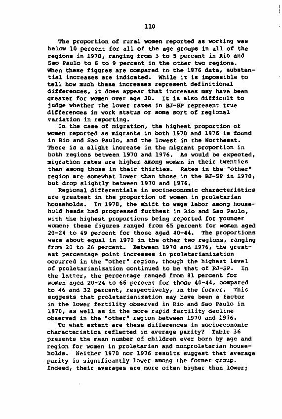
110

The proportion of rural women reported as working wasbelow 10 percent for all of the age groups in all of theregions in 1970, ranging from 3 to 5 percent in Rio andSao Paulo to 6 to 9 percent in the other two regions.When these figures are compared to the 1976 data, substan­tial increases are indicated. While it is impossible totell how much these increases represent definitionaldifferences, it does appear that increases may have beengreater for women over age 30. It is also difficult tojudge whether the lower rates in RJ-SP represent truedifferences in work status or some sort of regionalvariation in reporting.

In the case of migration, the highest proportion ofwomen reported as migrants in both 1970 and 1976 is foundin Rio and Sao Paulo, and the lowest in the Northeast.There is a slight increase in the migrant proportion inboth regions between 1970 and 1976. As would be expected,migration rates are higher among women in their twentiesthan among those in their thirties. Rates in the ·other·region are somewhat lower than those in the RJ-SP in 1970,but drop slightly between 1970 and 1976.

Regional differentials in socioeconomic characteristicsare greatest in the proportion of women in proletarianhouseholds. In 1970, the shift to wage labor among house­hold heads had progressed furthest in Rio and Sao Paulo,with the highest proportions being reported for youngerwomenJ these figures ranged from 65 percent for women aged20-24 to 49 percent for those aged 40-44. The proportionswere about equal in 1970 in the other two regions, rangingfrom 20 to 26 percent. Between 1970 and 1976, the great­est percentage point increases in proletarianizationoccurred in the ·other· region, though the highest levelof proletarianization continued to be that of RJ-SP. Inthe latter, the percentage ranged from 81 percent forwomen aged 20-24 to 66 percent for those 40-44, comparedto 46 and 32 percent, respectively, in the former. Thissuggests that proletarianization may have been a factorin the lower fertility observed in Rio and Sao Paulo in1970, as well as in the more rapid fertility declineobserved in the ·other· region between 1970 and 1976.

To what extent are these differences in socioeconomiccharacteristics reflected in average parity? Table 36presents the mean number of children ever born by age andregion for women in proletarian and nonpro1etarian house­holds. Neither 1970 nor 1976 results suggest that averageparity is significantly lower among the former group.Indeed, their averages are more often higher than 10werJ

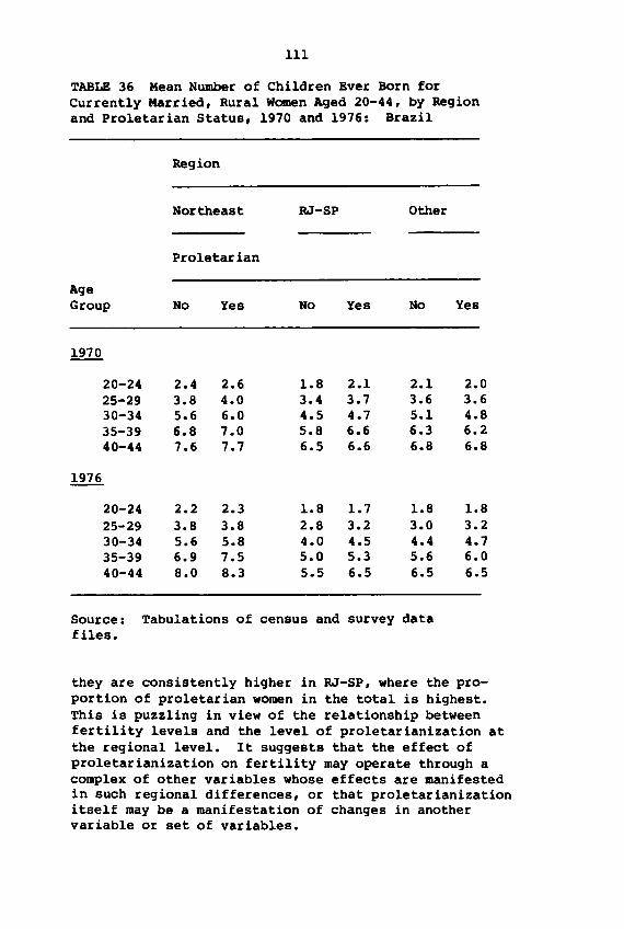
111

TABLE 36 Mean Number of Children Ever Born forCurrently Married, Rural Women Aged 20-44, by Regionand Proletarian Status, 1970 and 1976: Brazil

Region

Northeast RJ-SP Other

Proletarian

AgeGroup No Yes No Yes No Yes

1970

20-24 2.4 2.6 1.8 2.1 2.1 2.025-29 3.8 4.0 3.4 3.7 3.6 3.630-34 5.6 6.0 4.5 4.7 5.1 4.835-39 6.8 7.0 5.8 6.6 6.3 6.240-44 7.6 7.7 6.5 6.6 6.8 6.8

1976

20-24 2.2 2.3 1.8 1.7 1.8 1.825-29 3.8 3.8 2.8 3.2 3.0 3.230-34 5.6 5.8 4.0 4.5 4.4 4.735-39 6.9 7.5 5.0 5.3 5.6 6.040-44 8.0 8.3 5.5 6.5 6.5 6.5

Source: Tabulations of census and survey datafiles.

they are consistently higher in RJ-SP, where the pro­portion of proletarian women in the total is highest.This is puzzling in view of the relationship betweenfertility levels and the level of proletarianization atthe regional level. It suggests that the effect ofproletarianization on fertility may operate through acomplex of other variables whose effects are manifestedin such regional differences, or that proletarianizationitself may be a manifestation of changes in anothervariable or set of variables.

112

One such important variable may be work status. Table37 presents average parity for working and nonworkingwomen by age and region. The table suggests that averageparity was slightly lower for working women in theNortheast and ·other· regions in 1970, but not in Rio deJaneiro and Sao Paulo, there were so few working women inthe latter two states in 1970 that none of the averagesfor that group were significantly different from those ofnonworking women. In 1976, the pattern of differencesbetween working and nonworking women was even less clear:there were still no differences in RJ-SP, while working

TABLE 37 Mean Number of Children Ever Born for CurrentlyMarried, Rural Women Aged 20-44, by Region and WorkStatus, 1970 and 1976: Brazil

Region

Northeast RJ-SP Other

WorkingAgeGroup No Yes No Yes No Yes

1970

20-2425-2930-3435-3940-44

20-2425-2930-3435-3940-44

2.4 2.5 2.0 1.6 2.1 1.93.9 3.4 3.6 4.1 3.6 3.35.7 5.5 4.7 3.0 5.1 4.36.9 6.1 6.0 5.1 6.3 5.57.6 7.4 6.5 7.9 6.9 5.8

2.3 2.0 1.8 1.9 1.8 1.73.9 3.3 3.1 2.8 3.2 2.95.6 5.9 4.3 4.6 4.4 4.67.2 6.8 5.2 5.1 6.0 5.38.2 7.8 6.2 6.1 6.6 6.4

Source: Tabulations of census and survey data files.

113

women showed slightly lower averages for all but the age30-34 group in the other two regions. The lack of anydifference in the RJ-SP group and the reduction in the·other· group between 1970 and 1976 suggest that theeffect of work status on fertility differences is reducedas proletarianization increases. Another potentialcovariate is .igrationJ however, tabulations of averageparity by .igration status revealed no significantdifferences, and the results are not presented here.

This leads us back to education, which was the onlysocioeconomic characteristic of rural women for which aconsistent and statistically significant pattern of dif­ferences in average parity was observed. It is teaptingto conclude that education accounts for aost of the dif­ferentials, as well as the changes in rural fertilityobserved between 1970 and 1976. A proble. with the secondpoint is that levels of educational attainment increasedalmost equally during that period in the RJ-SP and ·other­regions, yet fertility decline was more rapid in thelatter. Either the evidence is only circuastantial thatrelative increases in proletarianization in that regionwere also greater, or there aay have been interactionbetween the education and proletarianization variables,and others as well. Since further presentation of datain tabular form would be an awkward way to address thisissue, that task is undertaken in the next chapter usingmultiple regressions.

CONCLUSIONS

The purpose of this chapter was to examine evidence onthe spread of contraceptive use to women in lower andmiddle socioeconomic classes who accounted for much ofthe acceleration in the decline of Brazilian maritalfertility in the early 1970s, focusing on changes in thesocioeconomic characteristics of these women that couldhave increased their aotivation to control fertility.Because there are no nationally representative data oncontraceptive use or socioeconomic characteristics, dataon contraceptive use from recent state-level surveys werepieced together, while changes in socioeconomic variablesand their relation to differences in average parity wereexamined based on 1970 census and 1976 PNAD survey datafiles.

Analysis of the proxiaate determinants of fertility inChapter 1 identified increased use of contraception (or

114

contraception combined with abortion) as a key factor inBrazil's accelerated fertility decline in the 1970s.Baseline data that would permit measurement of the extentto which this increase represepted the spread of fertilitycontrol among lower- and middle-income groups are lacking,however, data from contraceptive surveys taken later inthe decade show significant percentages of contraceptiveuse among these groups. This, along with evidence inChapter 2 showing that these groups experienced the mostrapid fertility decline during the decade, sUpPOrts theconclusion that their use of fertility control had indeedincreased. While Contraceptive Prevalence Surveys showthat differences in contraceptive use between higher andlower income and education groups remained, the percentageof use among the latter was far from negligible. Surveydata also show that organized family planning programscontributed to a reduction in socioeconomic class differ­entials in contraceptive use in a number of Northeasternstates.

This occurred during a period when significant changesin socioeconoaic conditions affecting the status of womenwere taking place in Brazil. The proportion of womenreporting no education was reduced, and there were signif­icant increases in the proportion reporting higher levelsof educational attainment in both urban and rural areas.Increased proportions of married women were also reportedas working, though it is difficult to determine to whatextent this reflects differences in the way census andsurvey data defined labor force participation. Increasedownership of consumer durables was observed among womenin urban households, while rural households were becomingincreasingly reliant on wage labor, or proletarianized.

Such changes are consistent with a number of hypothesesabout the reasons for increased motivation to controlfertility. Increases in educational attainment representa powerfUl modernizing force, and the relationship betweendifferences in average parity and education noted in thischapter is clearly very strong. However, this relation­ship was complicated by significant collateral changesrelating to increased economic pressures on low-incomeurban households and increases in rural proletarianiza­tion. The multivariate regression analysis in the nextchapter permits further examination of hypotheses linkingdifferences in average parity to these variables, as wellas a decomposition of changes in average parity from 1970to 1976 as they relate to changes in population composi­tion and in the impact of the different variables onfertility.

CHAPTER 4

ANALYSIS OF FERTILITY DETERMINANTS AT THE NATIONAL LEVEL

This chapter uses multivariate regression analysis toexplain how changes in average parity among married womenin Brazil relate to their changing socioeconomic charac­teristics during the accelerated fertility decline of theearly 1970s. In so doing, it attempts to provide a moresystematic assessment of the hyPOtheses presented in thelast two chapters, supported by tabular evidence, aboutsocioeconomic differences in fertility decline in Braziland the forces behind those differences.

The decision to focus on variability in the averageparity of married women was based on several considera­tions. First, fertility was measured according to averageparity rather than the last birth reported because of thequestionable reliability and comparability of the latterin studying changes over time among different socioeco­nomic groups. Second, analysis of the proximate deter­minants of the decline in the total fertility rate between1970 and 1976 indicated fertility control by married womento be the major factor involvedJ this conclusion was alsosupported by evidence on the diffusion of contraceptionamong new regions and income groups. Third, acceleratedfertility decline coincided with a number of importantsocioeconomic changes that could have had an impact on themotivation to control fertility, including increases infemale educational attainment and possible aggravation ofinflationary pressures on the economic resources of low­and middle-income households. The last two points sug­gested a working hyPOthesis about the acceleration offertility decline: that it was triggered by the conver­gence of two sets of forces--increased availability ofeffective means of contraception and the emergence ofsocioeconomic conditions conducive to smaller familynorms.

115

116

Because there is a lack of nationally representativedata combining information on contraceptive use and socio­economic characteristics, the analysis in this chapter islimited to the second set of forces. The principal ques­tion addressed is the extent to which the effects onreproductive behavior of such modernizing forces asincreased household income and female educational attain­ment (as measured by average parity) combined with otherfactors affecting household behavior, particularly thosereflecting such major structural dimensions of the Brazil­ian economy as inflation and income distribution. Differ­ential patterns of change among rural and urban areas sug­gested a division of the chapter into separate sectionsfor these groups, though work on the latter was even morerestricted by data limitations.

URBAN WOMEN

As noted earlier, the acceleration of fertility declinein Brazil coincided with a period during which lower- andmiddle-income urban households were raising their consump­tion expectations and beginning to realize them throughincreased purchases of housing and other consumer dur­ables, including televisions and automobiles, with mostpurchases made on the installment plan. Unequal treatmentof wages and credit obligations in Brazil's indexing sys­tem made it more difficult for families to keep up withpayments, and even to purchase basic necessities duringperiods of high inflation. As was suggested earlier,this, combined with increased knowledge of and access tocontraception, may have reduced family-size desires. Thisexplanation does not compete with a modernization frame­work, but extends it to incorporate other structuralchanges.

Among the research questions that need to be addressedare the following: (1) What measures in the availabledata files can be used as appropriate indices of the mod­ernizing forces and economic pressures discussed above?(2) How should the relationship between these measures andaverage parity be specified? Are the relationships lin­ear? Should interactions be taken into account? (3) Canthe analysis be pushed beyond explanation of differentialsin average parity in 1970 and 1976 to an assessment of thesOurces of change in fertility during that interval? Inother words, do declines in average parity reflect changesin the composition of the population of married women

117

according to modernizing characteristics, or is it more acase of changes in the parameters that reflect the impactof these variables on parity? The latter are likely toreflect structural changes, and one of the tasks here willbe to incorporate in the specification variables for whichsuch changes would be indicative of the specific struc­tural forces hypothesized above, that is, increased eco­nomic pressures on household resources.

It is important to recognize that questions in censusesand large-scale surveys do not provide a great deal ofconceptual precision for the measurement of modernizationand its influence on fertility. Most of the measures inthis chapter have appeared in the presentation of tabularevidence in earlier chapters, these include income andeducation, as well as age. A new variable that attemptsto measure households' relative economic positions hasalso been added.

Table 38 lists the variables that have been selectedfor the analysis of data on urban women. Variable labelsand a summary of variable definitions are shown. Averageparity (CEB) , the dependent variable, is listed first.In accounting for variation in this variable, the amountof exposure to the risk of conception needs to be con­trolled. This risk is associated with marital durationand maternal age. Data on age at marriage are providedonly in the 1976 data file, maternal age is a less satis­factory substitute, particularly at earlier ages whenthere is greater variability because the marriage isrecent. To maintain comparability between 1970 and 1976,regressions were run using maternal age (AGE) as a controlfor exposure to risk. Women were first separated intothree broad age categories, with AGE used as a controlvariable for each: (1) 20-24, (2) 25-34, and (3) 35-44.To test the sensitivity of results to marital duration(MOUR) , the 1976 data were then run using the AGE controlvariable.

The next two variables on the list relate to moderni­zation. It has become fairly standard practice in analy­tical approaches influenced by household economic theoryto use women's average educational attainment (MED) andtheir own and their husband's earnings (HINC) as variablesin analyzing differences in average parity (see Schultz,1976). Women's earnings and educational attainmentreflect the opportunity costs of childrearing vis-a-visother uses of their time, while the earnings of husbandsand wives measure their available resources for child­rearing and other activities. Theoretically, the effect

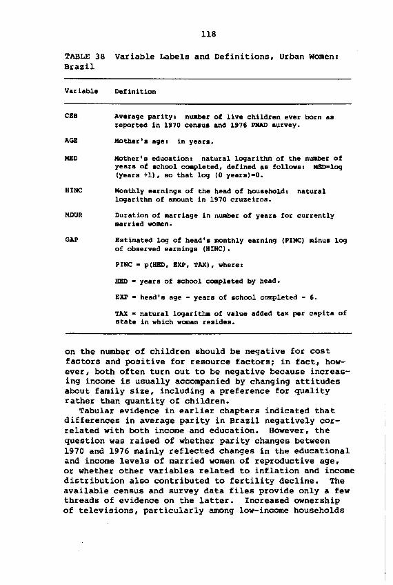
118

TABLE 38 Variable Labels and Definitions, Urban Women:Brazil

Variable Definition

CBB Average paritYI nuaber of live children ever born asreported in 1970 census and 1976 PNAD survey.

A~

MED

Mother's agel in years.

Mother's educationl natural logarithm of the number ofyears of school cc.pleted, defined as follows I MBD-log(years +1), so that log (0 years)-O.

HINC Monthly earnings of the head of household I naturallogarithm of amount in 1970 cruzeiros.

MDUR Duration of marriage in nuaber of years for currentlymarried women.

GAP Estimated log of head's monthly earning (PINe) minus logof observed earnings (HINe).

PINC - p(BED, EXP, TAX), where I

BED - years of school cc.pleted by head.

EXP - head's age - years of school completed - 6.

TAX - natural logarithm of value added tax per capita ofstate in which woman resides.

on the number of children should be negative for costfactors and positive for resource factors~ in fact, how­ever, both often turn out to be negative because increas­ing income is usually accompanied by changing attitudesabout family size, inclUding a preference for qualityrather than quantity of children.

Tabular evidence in earlier chapters indicated thatdifferences in average parity in Brazil negatively cor­related with both income and education. However, thequestion was raised of whether parity changes between1970 and 1976 mainly reflected changes in the educationaland income levels of married women of reproductive age,or whether other variables related to inflation and incomedistribution also contributed to fertility decline. Theavailable census and survey data files provide only a fewthreads of evidence on the latter. Increased ownershipof televisions, particularly among low-income households

119

likely to have purchased them on credit, suggests thatsuch factors could have been operative, increased femalelabor force participation suggests that economic pressuresmight have contributed to the delay or termination ofchildbearing.

However, exploratory attempts to incorporate televisionownership and female labor force participation in thespecification of the relationship between female educa­tional attainment, husband's earnings, and average parityyielded unsatisfactory results. The problem was in iden­tifying the endogenous effects of the employment and earn­ings of women in reproductive ages on their fertility,vis-a-vis the exogenous influence of those women's educa­tion and their husbands' earnings. The data files did notprovide other exogenous variables that could be used toestimate fully identified parameters for female employmentand earnings. Consequently, the analysis was limited toestimation of reduced-form coefficients, that is, onlyexogenous variables were included on the right-hand sideof the regression equation.

In view of this, and to permit continued pursuit of aspecification that would capture the effect of the rela­tive economic position of a woman's household (as well aspossible changes in that position) on her fertility, anapproach based on the concept of relative income wasadopted. A household's income is relative in that it maybe greater or less than the income stream that would beexpected on the basis of that househOld's human capitalendowments. A gap between observed and expected income,if it existed, would indicate whether a household was moreor less vulnerable to outside economic pressures such asinflation. The approach is consistent with Leibenstein's(1974) point about the relationship between income andfertility: that while the overall relationship may benegative, it may be positive within specific referencegroups, with higher fertility among higher-income house­holds within a particular group.

This approach was operationalized by first estimatingthe expected earnings of husbands using standard earningsequations, and then determining what each husband's earn­ings would be given his partiCUlar characteristics. Theestimates were based on husband's earnings rather thanhousehold income for simplicity's sake (estimates couldthen be based on the characteristics of one individualwithout consideration of household size and structure aswell as other income sources). Some of the limitationsof this approach are offset by the fact that the analysis

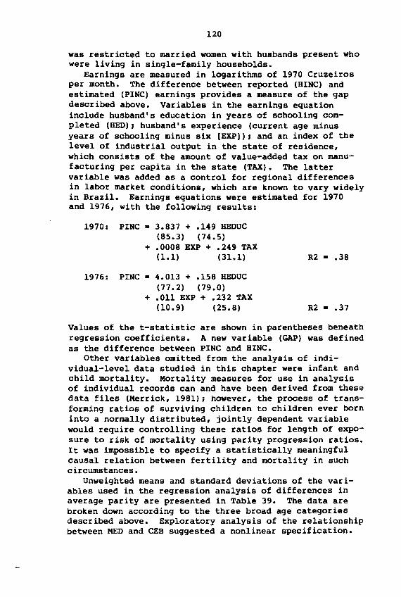
120

was restricted to married women with husbands present whowere living in single-family households.

Earnings are measured in logarithms of 1970 Cruzeirosper month. The difference between reported (HINC) andestimated (PINC) earnings provides a measure of the gapdescribed above. Variables in the earnings equationinclude husband's education in years of schooling com­pleted (HED), husband's experience (current age minusyears of schooling minus six [EXP), and an index of thelevel of industrial output in the state of residence,which consists of the amount of value-added tax on manu­facturing per capita in the state (TAX). The lattervariable was added as a control for regional differencesin labor market conditions, which are known to vary widelyin Brazil. Earnings equations were estimated for 1970and 1976, with the following results:

1970: PINC. 3.837 + .149 HEDUC(85.3) (74.5)

+ .0008 EXP + .249 TAX(1.1) (31.1)

1976: PINC· 4.013 + .158 HEDUC(77.2) (79.0)

+ .011 EXP + .232 TAX(10.9) (25.8)

R2 • .38

R2 • .37

Values of the t-statistic are shown in parentheses beneathregression coefficients. A new variable (GAP) was definedas the difference between PINC and HINC.

Other variables omitted from the analysis of indi­vidual-level data studied in this chapter were infant andchild mortality. Mortality measures for use in analysisof individual records can and have been derived from thesedata files (Merrick, 1981), however, the process of trans­forming ratios of surviving children to children ever borninto a normally distributed, jointly dependent variablewould require controlling these ratios for length of expo­sure to risk of mortality using parity progression ratios.It was impossible to specify a statistically meaningfulcausal relation between fertility and mortality in suchcircumstances.

Unweighted means and standard deviations of the vari­ables used in the regression analysis of differences inaverage parity are presented in Table 39. The data arebroken down according to the three broad age categoriesdescribed above. Exploratory analysis of the relationshipbetween MED and CEB suggested a nonlinear specification.

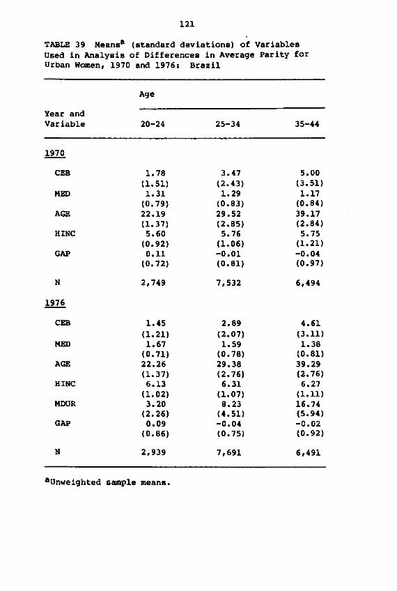
121

TABLE 39 Meansa (standard deviations) of VariablesUsed in Analysis of Differences in Average Parity forUrban Women, 1970 and 1976: Brazil

Age

Year andVariable 20-24 25-34 35-44

1970

CEB 1.78 3.47 5.00(1.51) (2.43) (3.51)

MED 1.31 1.29 1.17(0.79) (0.83) (0.84)

AGE 22.19 29.52 39.17(1.37) (2.85) (2.84)

HINC 5.60 5.76 5.75(0.92) (1.06) (1.21)

GAP 0.11 -0.01 -0.04(0.72) (0.81) (0.97)

N 2,749 7,532 6,494

1976

CEB 1.45 2.89 4.61(1.21) (2.07) (3.11)

MED 1.67 1.59 1.38(0.71) (0.78) (0.81)

AGE 22.26 29.38 39.29(1.37) (2.76) (2.76)

HINC 6.13 6.31 6.27(1.02) (l.07) (1.11)

MDUR 3.20 8.23 16.74(2.26) (4.51) (5.94)

GAP 0.09 -0.04 -0.02(0.86) (0.75) (0.92)

N 2,939 7,691 6,491

aUnweighted sample means.

122

Consequently, NED was defined as the logarithm of awoman's years of schooling completed plus one, so thatthe logarithm of zero years of schooling would equalzero. As indicated above, RINe is also measured inlogarithms.

Since GAP is the residual of the estimated value ofRINe, it has a zero mean for the total study population,but varies slightly from zero in specific age categories.Current earnings of husbands of younger women averagedslightly higher than their estimated earnings, while theaverage GAP for older women fell slightly below zero. Itshould also be noted that there are significant negativecorrelations f.7 to .8) between RINe and GAP, this indi­cates a tendency for current earnings to be lower thanexpected earning among husbands with lower earninglevels, and for current earnings to exceed expected earn­ings by larger amounts among husbands with higher earn­ings. A check of outliers in the earnings equationsindicated that these high zero order correlations were astatistical artifact produced by cases at extremes of theincome distribution: overestimation of earnings whenhusbands reported zero earnings and underestimation whenthey reported very high earnings. These correlationsdisappeared when extreme cases were omitted, however, itwas decided not to exclude such cases from the analysisof fertility differentials because the impact of the dif­ferential between RINe and PINe was of interest over theentire range of the income distribution.

The data in Table 39 on average marital duration fMDUR)in 1976 suggest that analysis of fertility differentialsamong younger women is likely to be quite sensitive todifferences in exposure to the risk of conception becauseof the selectivity within that age group toward women whomarried early. The average age at marriage for women aged20-24 in 1976 was 19.1 years, compared to 21.1 years forwomen aged 25-29. Relative variation in MOOR is alsogreater among younger women: the coefficient of variationfor that group was 71 percent compared to 55 percent for25-34 and 35 percent for 35-44. Caution is suggested ininterpreting results for the youngest age category whenMOOR cannot be controlled.

Analysis of Urban CEB Differentials in 1970 and 1976

Results of ordinary least squares regression analysis ofdifferences in CEB for women grouped by broad age cate-

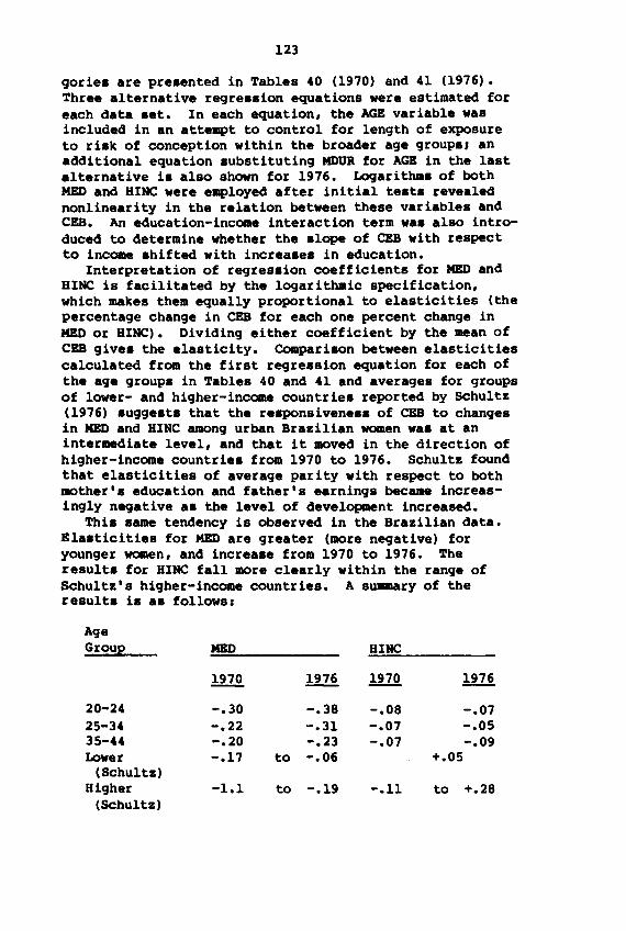
123

goriea are preaented in Tables 40 (1970) and 41 (1976).Three alternative regreaaion equations were estimated foreach data aet. In each equation, the AGE variable wasincluded in an attempt to control for length of exposureto riak of conception within the broader age groupa, anadditional equation aubstituting MOOR for AGE in the lastalternative ia also shown for 1976. Logarithaa of bothNED and HIMe were employed after initial teata revealednonlinearity in the relation between these variables andCBB. An education-income interaction term waa also intro­duced to determine whether the alope of CEB with respectto income ahifted with increaaea in education.

Interpretation of regresaion coefficients for NED andHINC is facilitated by the logarithaic specification,which makes them equally proportional to elasticities (thepercentage change in CEB for each one percent change inNED or HIMe). Dividing either coefficient by the mean ofCBB givea the elasticity. Compariaon between elasticitiescalculated from the first regreasion equation for each ofthe age groupa in Tables 40 and 41 and averages for groupsof lower- and higher-income countriea reported by Schultz(1976) auggeata that the reaponsiveneaa of CEB to changesin NED and HINC among urban Brazilian women waa at anintermediate level, and that it moved in the direction ofhigher-income countriea from 1970 to 1976. Schultz foundthat elasticities of average parity with respect to bothmother'a education and father's earnings became increas­ingly negative aa the level of development increased.

Thia a&me tendency is observed in the Brazilian data.Elaaticities for NED are greater (more negative) foryounger women, and increaae from 1970 to 1976. Theresulta for HIMe fall more clearly within the range ofSChultz's higher-income countries. A summary of theresulta ia aa follows:

NED HINC

ll1Q. !ill ll1Q. !ill

-.30 -.38 -.08 -.07-.22 -.31 -.07 -.05-.20 -.23 -.07 -.09-.17 to -.06 +.05

-1.1 to -.19 -.11 to +.28

20-2425-3435-44Lower

(SChultz)Higher

(SChultz)

AgeGroup

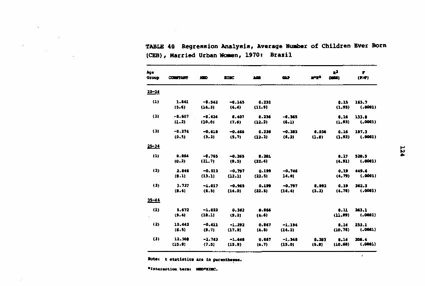
TABLE 40 Recjression Analysis, Average Hu.ber of Children Ever Born

(CBS), Married Urban WOIMn, 1910, Brazil

Alga .a rGroup ~ JIll) UK IGIII au .... e-I (F.>I'I

lJ!::U

(11 1.ln -0.542 -I.U5 o.au 0.15 113.7(5.61 (U.31 (t.tl (11.'1 (l.151 (.00011

(2) -0.107 -O;Ut 0.t07 0.236 -1.315 0.11 133.1(l.al (l0.0) (7.61 (12.al (6.11 (1.'31 (.00011

(3) -o.an -I.UI -I.til o.aH -1.313 1.031 0.11 107.3(0.51 (3.a) (5.71 (la.al (6.al (l.I) (l.U) (.00011

35-3t~

'"(1) 0.0" -1.765 -1.215 1.201 0.17 520.5 •(o.a) (U.71 ('.51 (aa.tl (t.'l1 (.00011

(a) a.lu -0.513 -1.717 O.lft -I.7U 0.11 ....6(1.11 (13.11 (12.11 (U.51 U.II (t.7I1 (.00011

(3) 3.727 -1.017 -I.K5 O.lft -1.717 1.012 0.11 Ha.3(I.t) (6.51 (U.OI (u.6) (U.t) (3.31 (t.71) (.00011

35-..

(11 5.na -1.0aa O.Ha I.OM o.u 213.1(•• tl (l1.1) (•• al (t.6) (U.OII (.00011

(2) 1O...a -0.611 -l.21a o.on -l.lIt O.lt a53.1(6.5) ('.7) (17.0) (t.1) (u.a) (10.76) (.00011

(3) 12.301 -1.7U -1."1 o.on -1.311 0.203 o.U 2OI.t(l5.1) (7.51 (l5.I) (t.71 (15.01 (5.1) (10.111 (.00011

1Iote. t atatiatica ara in parentbe~.

aInte~action te~. 1IID"JII.c•

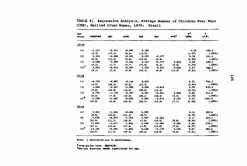
TABLE 41 Regression Analysis, Average Number of Children Ever Born(CBB) , Married Urban Women, 1976: Brazil

Age .2 PGroup COItSTAIlT IIBD BIRe llGB GAP N-Be (1IiIB) (P>P)

--~

(1) -1.137 -0.552 -0.097 0.184 0.16 186.4(3.3) (17.3) (4.4) (12.2) (1.27) (.0001)

(2) 0.334 -0.400 -0.381 0.187 -0.377 0.18 161.5(0.9) (11.0) (9.6) (12.6) (8.6) (1.24) (.0001)

(3) -0.098 -0.288 -0.341 0.187 -0.372 0.019 0.18 129.3

(4)b(0.2) (1.7) (4.7) (12.6) (8.3) (0.6) (1.24) (.0001)3.043 -0.414 -0.387 0.322 -0.241 0.045 0.47 50,.8

(9.1) (3.0) (6.6) (42.3). (6.6) (11.9) (0.81) (.0001)

25-34 ....-- N

-0.754 0.203 0.23 758.2U1(1) -0.887 -0.143

(3.0) (28.2) (6.5) (27.3) (3.40) (.0001)(2) 1.659 -0.657 -0.5'9 0.206 -0.615 0.25 635.9

(5.6) (18.8) (15.6) (28.0) (14.4) (3.31) (.0001)(3) 2.729 -1.178 -0.787 0.207 -0.651 0.088 0.25 512.0

(6.4) (7.8) (12.0) (28.1) (14.9) (3.5) (3.30) (.0001)(4)b 6.538 -1.300 -0.822 0.244 -0.519 0.154 0.43 1441.2

(20.0) (9.9) (14.4) (59.3) (13.6) (7.1) (2.52) (.0001)

~

(1) 5.403 -1.040 -0.422 0.085 0.14 360.6(9.8) (19.6) (11.5) (6.5) (8.70) (.0001)

(2) 9.659 -0.678 -1.253 0.097 -1.082 0.17 323.3(15.6) (11.7) (18.4) (7.6) (14.4) (8.8) (8.45) ( .0001)

(3) 13.004 -2.437 -1.842 0.099 -1.263 0.295 0.18 278.1(17.1) (10.2) (17.8) (7.8) (16.0) (7.5) (8.37) (.0001)

(4)b 14.164 -2.546 -1.882 0.168 -1.179 0.330 0.27 483.2(25.0) (11.3) (19.4) (30.2) (16.0) 19.0) (7.51) ( .0001)

Hot•• t .teti.tic••r. in per.nth.....

-Interaction t.ra. IIBD-BIRe.~ritel duretion (HDOR) .ubetituted for 89••

126

At 1970 mean levels of KED and CBB, the 48 percent in­crease in the average number of years of schoolingachieved by women in the 25-34 age group (recalling thatMED • log [years of school + 1) would account for an 11percent decline in CBB. While these results suggest thatBrazilian experience during the early 1970s was consistentwith patterns observed among lower-middle income coun­tries, the elasticities of CEB with respect to father'searnings appear to lean more toward the negative valuescharacteristic of higher-income countries than do thosefor MED.

One reason for this could be the earnings gap hypothe­sis discussed above: that the effects of earnings on CEBcan be positive within a given reference group even if theoverall relation between CEB and HINC is negative. Thesecond set of regression equations, which incorporates theGAP variable, confirms this. The regression coefficientfor GAP is negative, implying that the more husband'sestimated earnings (PINC) exceed actual earnings (HINC),the lower is the average observed CEB. In a society likeBrazil in which income differentials are associated witha variety of sociocultural factors that could influencereproductive behavior, it makes sense to look for theeffect of income on fertility within rather than betweenspecific reference groups.

Similar considerations raise the question of whetheran interaction with sociocultural factors associated withdifferences in educational attainment affects the regres­sion results for KED and HINC. The third set of regres­sion equations includes an interaction term. This termis statistically significant in both 1970 and 1976 forwomen in the 25-34 and 35-44 age groups because of thelarge sample sizel addition of the variable affects onlythe third digit of R-square. The term's positive signindicates that with increases in MED, the negative impactof HINC on CEB is attenuated, as is the effect of MED asHINC increases. This is what one would expect given thevariety of sociocultural influences described earlier.

As noted above, the variable AGE was included in allthree variants of the regression equations as a controlfor differences in the risk of exposure to conceptionwithin each of the broader age groups. Marital durationis a better measure of such risk, but was not included inthe 1970 census. However, it was incorporated in the 1976survey, and equation (4) in Table 41 substitutes MOUR forAGE to provide some measure of the effect of using AGE asthe measure of exposure to risk. As one would expect, AGE

127

appears to be least satisfactory for younger women, forwhom both absolute and relative variation in CEB was moresensitive to MOUR than AGE. It is interesting to notethat while the coefficients for KED and HINC increased innegative magnitude with the addition of MOUR, the impactof GAP was reduced, this suggests that the effect on CEBof the relative status captured by GAP may be tied tomarital duration. Among younger women whose husband'searnings fall below the expected level, lower CEB couldbe the result of longer intervals between marriage andfirst birth, a point that deserves further exploration.

Concern about MOUR is warranted because of its impli­cations for interpreting changes in CEB from 1970 to 1976.The extent of this concern will depend on one's confidencein the conclusions derived earlier from census and surveydata: that average ages at marriage and first birth didnot change substantially between 1970 and 1976, and thatmost of the decline in total fertility can be attributedto a decline in marital fertility rather than to changesin the proportions married. The issue is less importantto determining how much changes in socioeconomic statuscontributed to declines in CBB than to examining how thosechanges were translated into declines via the proximatedeterminants of fertility.

Sources of Change in CEB from 1970 to 1976

Regression analyses of differences in CEB also can be usedto identify sources of change in CEB from 1970 to 1976.As noted earlier, an important question is whether suchchange resulted from a redistribution of women accordingto socioeconomic characteristics or from a shift in theparameters relating these characteristics to CBB. Oneapproach is to evaluate the regression coefficientsreported in Tables 40 and 41 using sample means, and thenexamine changes in the contribution of each variable tothe level of CEB for the two dates. With two sets ofregression results, there are three ways that one canproceed: forward using 1970 coefficients with means forboth dates, backward using 1976 coefficients with bothsets of means, or by comparing means and coefficients foreach date. Changes in the average value of CEB could bethe result of changes in educational attainment or othervariables included in the regressions, changes in regres­sion coefficients, or shifts in conditions that are notmeasured, but are reflected in the constant term. The

128

first two variants of this approach hold the coefficientsconstant, but will give different results to the extentthat coefficients have changed, by definition there is nochange in the constant term. The third variant allows forchange in the constant, but confuses changes in composi­tion with shifts in coefficients. An alternative approachis to reestimate coefficients and include bOth a dummyvariable for time to capture shifts in the constant term,and interaction terms for time and each of the variablesin the regression to measure changes in regression coef­ficients. The new estimators can then be evaluated atbOth sets of sample means to determine the contributionof changes in composition to observed changes in the levelof CED. Both of these approaches have been attempted.

Table 42 presents the first approach: the first columnrepresents changes with the 1970 regressions, the secondcolumn represents changes with the 1976 regressions, andthe third column shows the difference between the evalua­tion of 1970 regressions with 1970 means and the 1976regressions with 1976 means. The third set of regressionsin Tables 41 and 42 (with the interaction term) was usedfor the two older age categories where interactions weresignificant. The total of changes in each group of coef­ficients adds to the estimated change in CED for thatgroup, by definition, the estimated change in CEB equalsthe actual change in the last column.

In the first two variants, estimated changes exceed theactual in all cases, especially using the 1970 coeffici­ents and in the case of older women, this suggests somecombination of change in coefficients and in the constantterm. Changes in the average level of husbands' earningsappear to have had a greater impact than maternal educa­tion, more so in 1970 than in 1976, which suggests anattenuation in the importance of the earnings effect. Animportant fraction of the negative effects of KED and HINCis offset by the positive KED*HINC interaction term. Com­pared to KED and HINC, changes in the GAP variable hadlittle effect, in fact, a slight narrowing of the averageGAP contributed a slightly positive impetus to averageCBB. Shifts in age composition also raised CEB for olderwomen.

The third variant is useful mainly in illustrating howthe combined effects of changes in composition and incoefficients relate to changes when coefficients are heldconstant. For example, the effect of changes in the HINCcoefficient and the average level of HINC would have con­tributed to an increase of .562 in CEB among women aged

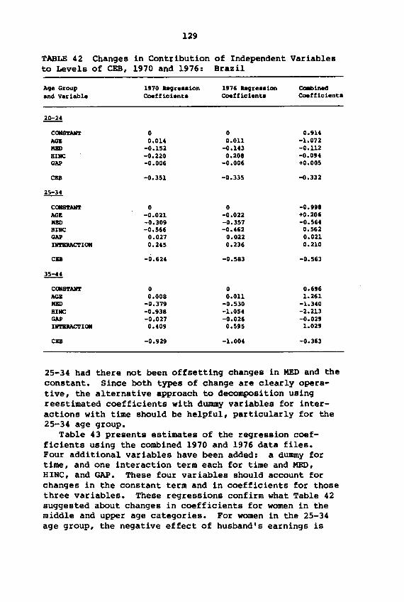
129

TABLE 42 Changes in Contribution of Independent Variablesto Levels of CED, 1970 and 1976: Brazil

Age Group 1970 -.grea81on 1976 -.gre.81on COIIbinedand Variable Coefficiente Coefficient. Coefficiente

.!!!::l!

COIISTAIft' 0 0 0.914AGE 0.014 0.011 -1.072MBD -0.152 -0.143 -0.112BIHC -0.220 0.208 -0.094GAP -0.006 -0.006 +0.005

CD -0.351 -0.335 -0.332

~

COIISTAIft' 0 0 -0.998AGE -0.021 -0.022 +0.206MBD -0.309 -0.357 -0.564BIHC -0.566 -0.462 0.562GAP 0.027 0.022 0.021UITBlIAC'l'IOII 0.245 0.236 0.210

CBB -0.624 -0.583 -0.563

~

COII8'1'AIIT 0 0 0.696AGE 0.008 0.011 1.261MBD -0.379 -0.530 -1.340BIHC -0.938 -1.054 -2.213GAP -0.027 -0.026 -0.029III'l'BRACTIOII 0.409 0.595 1.029

CBB -0.929 -1.004 -0.363

25-34 had there not been offsetting changes in KED and theconstant. Since both types of change are clearly opera­tive, the alternative approach to decomposition usingreestimated coefficients with dummy variables for inter­actions with time should be helpful, particularly for the25-34 age group.

Table 43 presents estimates of the regression coef­ficients using the combined 1970 and 1976 data files.Four additional variables have been added: a dummy fortime, and one interaction term each for time and MED,HINC, and GAP. These four variables should account forchanges in the constant term and in coefficients for thosethree variables. These regressions confirm what Table 42suggested about changes in coefficients for women in themiddle and upper age categories. For women in the 25-34age group, the negative effect of husband's earnings is

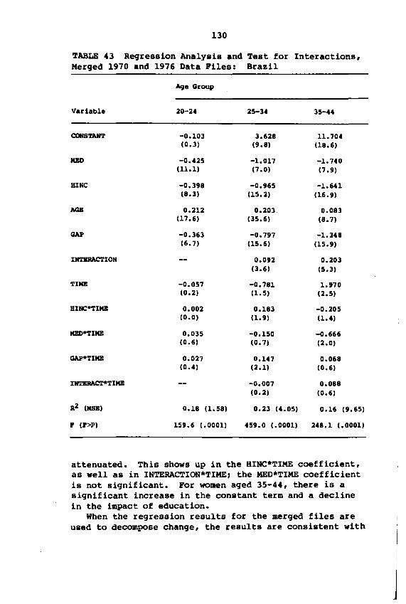
130

TABLE 43 Regression Analysis and Test for Interactions,Merged 1970 and 1976 Data Files: Brazil

Age Group

Variable 20-24 25-34 35-44

COIISTAII'1' -0.103 3.628 ll.704(0.3) (9.8) (18.6)

NED -0.425 -1.017 -1. 740(ll.l) (7.0) (7.9)

B1NC -0.398 -0.965 -1.641(8.3) (15.2) (16.9)

10GB 0.212 0.203 0.083(17.6) (35.6) (8.7)

GAP -0.363 -0.797 -1.348(6.7) (15.6) (15.9)

IIITBRACTION 0.092 0.203(3.6) (5.3)

TIME -0.057 -0.781 1.970(0.2) (1.5) (2.5)

BINC*TIMB 0.002 0.183 -0.205(0.0) (1.9) (1.4)

MBD*TIMB 0.035 -0.150 -0.666(0.6) (0.7) (2.0)

GAP*TIMB 0.027 0.147 0.068(0.4) (2.1) (0.6)

IIITBRACT*TIMB -0.007 0.088(0.2) (0.6)

R2 (MSB) 0.18 (1.58) 0.23 (4.05) 0.16 (9.65)

F (F>P) 159.6 (.0001) 459.0 (.0001) 248.1 (.0001)

attenuated. This shows up in the HINC*TlME coefficient,as well as in INTERACTION*TIMEJ the MED*TIME coefficientis not significant. For women aged 35-44, there is asignificant increase in the constant term and a declinein the impact of education.

When the regression results for the merged files areused to decompose change, the results are consistent with

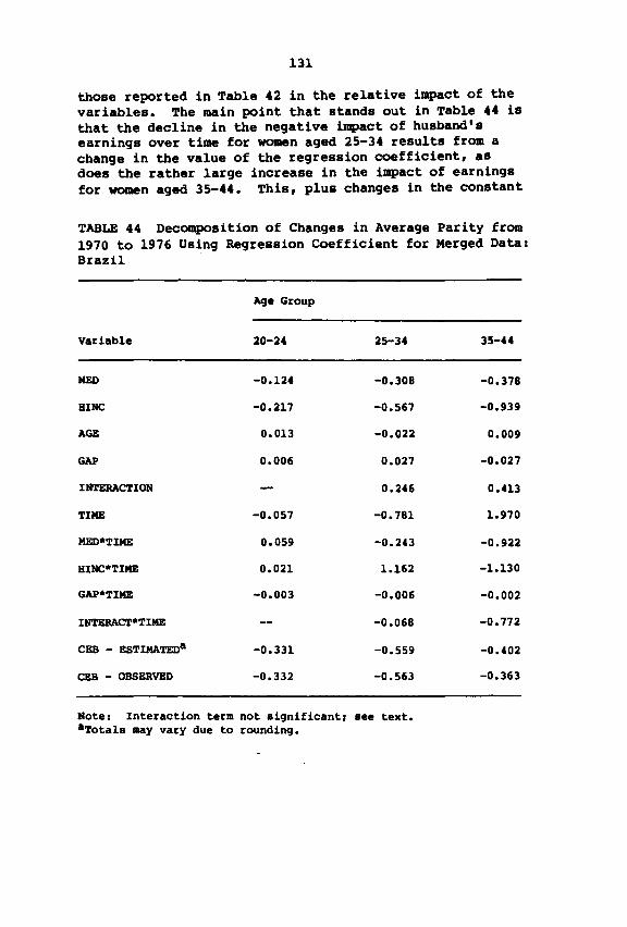
131

those reported in Table 42 in the relative impact of thevariables. The main point that stands out in Table 44 isthat the decline in the negative impact of husband'searnings over time for women aged 25-34 results from achange in the value of the regression coefficient, asdoes the rather large increase in the impact of earningsfor women aged 35-44. This, plus changes in the constant

TABLE 44 Decomposition of Changes in Average Parity from1970 to 1976 Using Regression Coefficient for Merged Data:Brazil

Age Group

Variable 20-24 25-34 35-44

NED -0.124 -0.308 -0.378

BINe -0.217 -0.567 -0.939

AGE 0.013 -0.022 0.009

GAP 0.006 0.027 -0.027

INTERACTION 0.246 0.413

TIME -0.057 -0.781 1.970

NED*TIME 0.059 -0.243 -0.922

BINe*TIME 0.021 1.162 -1.130

GAP*TIME -0.003 -0.006 -0.002

INTERACT*TIME -0.068 -0.772

eBB - BSTIMATEDa -0.331 -0.559 -0.402

CBB - OBSBRVED -0.332 -0.563 -0.363

Note I Interaction term not significantl see text.aTota1s may vary due to rounding.

132

term (as reflected in the change attributed to TIME) ,suggests that some important structural shifts accompaniedthe changes in composition by MED and HINC and contributedto declines in CBB.

What is puzzling is that these shifts do not show upin the GAP variable, Which, despite its importance inexplaining differentials in CEB, does not appear to COn­tribute much to changes in CEB between 1970 and 1976. Onereason for this could be that changes in the average levelof GAP are not the appropriate place to be looking for theeffects of changes transmitted through that variable. GAPwas introduced to measure the effect of inflationary con­ditions and changes in the distribution of earnings on theeconomic position of households. Therefore, changes inthe average level of GAP should be less relevant thanchanges in its distribution.

Table 45 examines changes in the distribution of GAPbetween 1970 and 1976 and indicates the possible impactof such changes on CEB. The table shows the percent ofwomen in each age category, broken down by deciles offamily income, residing in families whose husband's earn­ings fall more than one standard deviation from the meanlevel of GAP for that age group. The table also shows inparentheses the relative weight (as a percent of all womenin the age group) of these women in total CBB. These datasuggest that for certain groups (e.g., ages 25-34 inmiddle-income deciles) there may have been a greater dis­persion of GAP in 1976. However, the table also showsthat this increase in dispersion was probably not greatenough to have made a major difference in changes in theaverage level of CBB over the period under study. In thisconnection, it is important to note that the relativeearnings effect expressed in GAP does appear to make adifference in the explanation of differentials in CEB inboth 1970 and 1976. The point is that GAP (and the struc­tural changes it measures, perhaps quite inadequately)does not appear to account for much of the change in CEBbetween 1970 and 1976.

Thus our assessment of the components of changes in CEBfrom 1970 to 1976 indicates that increases in the educa­tional attainment of married women in Brazil and increasesin their husbands' earnings contributed significantly tothe decline of average CEB. At the same time, structuralchange is not ruled out. Clearly, the role of that changeis suggested by the significant and somewhat erraticshifts in the values of the regression coefficients forHINC, as well as changes in the constant terms in regres-

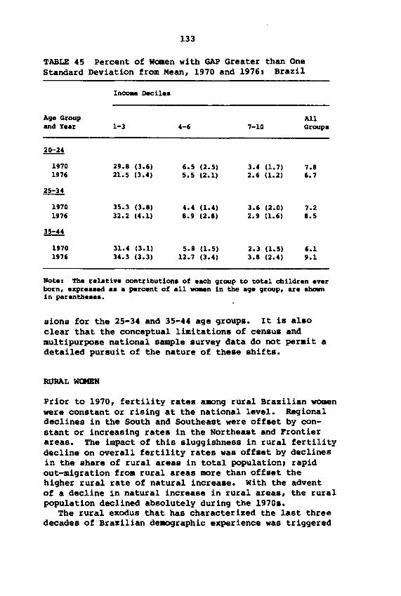
133

TABLE 45 Percent of Women with GAP Greater than OneStandard Deviation from Mean, 1970 and 1976: Brazil

InCOM Decil••

Age Group Alland Y.ar 1-3 4-6 7-10 Group.

20-24

1970 29.8 (3.6) 6.5 (2.5) 3.4 (1.7) 7.81976 21.5 (3.4) 5.5 (2.1) 2.6 (1.2) 6.7

~

1970 35.3 (3.8) 4.4 (1.4) 3.6 (2.0) 7.21976 32.2 (4.1) 8.9 (2.8) 2.9 (1.6) 8.5

ll=!!

1970 31.4 (3.1) 5.8 (1.5) 2.3 (1.5) 6.11976 34.3 (3.3) 12.7 (3.4) 3.8 (2.4) 9.1

Rot. I The r.1ativ. contribution. of .ach group to total childr.n .v.rborn, .xpr••aed a. a percent of all ~n in the ag. group, ar••bownin par.nth•••••

sions for the 25-34 and 35-44 age groupa. It is alaoclear that the conceptual limitations of cenaua andmultipurpose national sample aurvey data do not permit adetailed pursuit of the nature of theae shifts.

RURAL W<»tEN

Prior to 1970, fertility rates among rural Brazilian womenwere constant or rising at the national level. Regionaldeclines in the South and Southeast were offaet by con­stant or increasing rates in the Northeaat and Prontierareas. The impact of this sluggishness in rural fertilitydecline on overall fertility rates was offaet by declinesin the share of rural areas in total population, rapidout-migration from rural areas more than offset thehigher rural rate of natural increaae. with the adventof a decline in natural increase in rural areaa, the ruralpopulation declined absolutely during the 1970a.

The rural exodus that has characterized the last threedecades of Brazilian demographic experience was triggered

134

by a cOlllbination of aocial, economic, and politicalforces, many of them longatanding features of ruralBrazilian society. One of the most basic of these is thecOlllbination of a limited supply of good land and increas­ing population pressurer droughts and infertile soil haveplagued areas with a high concentration of rural popula­tion, particularly in the Northeaatern states. A secondforce is the unequal distribution of land, with substan­tial proportions of rural familiea being forced to eke asubsistence out of minifundia holdings of fewer than fivehectares. A third ia that there has been increased con­solidation of land holdings accompanying the commerciali­zation of Brazilian agriculturer this process has receivedadditional stimulua from the energy crisis and Brazil'sresultant need to raise foreign exchange through agricul­tural exports and increase production of alcohol as a sub­stitute for petroleum imports. This lack of opportunityin rural areas, combined with hopes of paid employment andurban amenitiea, has motivated Brazil'a rural-urbanmigration.

While migration was the primary demographic responseto adverse socioeconomic conditions among the masses ofBrazil's rural population, other demograhic processes wereaffected, inclUding fertility and family formation. Chap­ter 3 suggested several hypotheses about how such changesmight be affecting rural fertility in Brazil. All focusin one way or another on the role of children as bothimmediate productive resources and longer-term investmentsfor rural families, and on how changes in rural socioeco­nomic and institutional conditions could have affectedthis role.

One hypothesis relates to land availability. As theamount of land available to farm families in more denselysettled areas is reduced, several forces that could moti­vate not only out-migration, but also lower fertility areset in motion. Por families remaining in agriculture thatwish to transmit land to their children through inherit­ance, large numbers of children will lead to an uneco­nomical subdivision of plotsJ this can be avoided only byhaving fewer children, forcing children to start their ownfamilies later, or encouraging the children's migration.The value of children as immediate productive resourceswill also be affected to the extent that smaller plotsreduce the need for child labor.

The influence of these forces on reproductive behavioris mediated by institutional factors and by the availabil­ity of new land in other areas. Research on land avail-

135

ability and fertility in rural Brazil using data from the1970 censuses of population and agriculture found thatfertility was lower in more densely settled regions ofSoutheastern Brazil and higher in areas of new rural set­tlement in the Central-Western region (Merrick, 1974).An extension of that research to Northeastern Brazil andto the frontier settlements in the Amazon region did notreveal similar patterns (Merrick, 1981). Several reasonsfor this were suggested, Amazon settlement really did notget underway until after 1970, and the very unequal dis­tribution of access to land in the Northeast was not asconducive to the pattern observed in the SOuth, here ahigher proportion of family faras were owner-operated.

Research with 1970 data also revealed the very severelimitations of population census data for dealing withlinks between rural demographic changes and socioeconomicand institutional factors affecting those changes. Theselimitations were overcome to some extent by combining pop­ulation census data with information from the agriculturalcensus. Analysis of changes during the 1970s will haveto await the availability of detailed information from the1980 censuses of agriculture and population. Unfortu­nately, the PNAD surveys taken during the 1970s do notprovide the geographic detail required for linking themto results of the 1975 agricultural census, moreover, .thePNAD sample does not include rural areas of the Central­West and Amazon regions, so that the potential positiveeffects on fertility of frontier settlement in thoseregions during the 1970s cannot be examined.

Some features of the relationship between fertilitydecline in rural Brazil during the 1970s and socioeconomicchange in the areas included in the PNAD surveys can bestudied. One of these relates to an institutional factormediating the response to increasing economic pressures,such as scarcity of land and consolidation of land inlarger holdings, on the demographic responses of farmfamilies. This factor is rural proletarianization, or theshift from an owner-operator and farm family labor modeof production to wage labor. As noted earlier, Europeanexperience, as well as evidence from SOuthern Brazil,indicates that lower fertility is more likely to resultfrom a scarcity of land when farm families own their landand reduced fertility allows them to maintain control ofthe land. Rural proletarianization weakens this motiva­tion. As noted in Chapter 3, Paiva (1982) disagrees withthis interpretation for Brazil. He argues that prole­tarianization reduces the value of children as farm

136

laborers and provides incentivea for reduced fertility,including increased market work for both women and chil­dren. The potential value of market work would beincreased by education, and by a ahift toward qualityrather than quantity of children.

The data with which to evaluate theae two interpreta­tions of Brazilian experience are scant. Tabular evidencepreaented in Chapter 3 indicated that average parity wasindeed lower in regions with higher levels of proletarian­ization (meaaured according to the proportion of ruralhousehold heads reported as employeea), in the sametablea, however, average parity was higher rather thanlower for proletarian households within thoae regions.While one must be careful to avoid the fallacy of compo­sition, one must also be careful about biaa arising fromthe location of families when their characteristics havebeen measured in census and survey data. For rural areas,those data detect only that proportion of the proletar­ianized population remaining at the time interviews wereconducted, those who moved (either to urban areas or toother rural areaa) and who may well have had lower fer­tility would not be included.

Another aSPeCt of change in rural fertility relates tothe socioeconomic differentials observed in Chapter 2.While these differentials were not as great as thoseobserved in urban areas, the data presented in Chapters 2and 3 indicated that rural women with some education hadlower fertility than those with no education, and that theproportion of rural women with some education increasedfrom 1970 to 1976. Also, rural women with no educationas a percent of all women aged 15-49 declined from about21 percent to about 13 percent, a result of some combina­tion of increases in educational attainment among ruralwomen, out-migration, and possible underrepresentation ofless-educated rural women in the PNAD survey. Such evi­dence suggests that the role of education should, not beneglected in examining rural fertility differences.

Analysis of Rural CEB Differentials in 1970 and 1976

As indicated above, neither the 1970 census nor the 1976PNAD survey provides many meaningful measures of conceptsrelevant to the analysis of changes in rural fertility inBrazil. The multivariate analysis that follows is pre­sented primarily to illustrate how the relationshipsbetween differences in average parity and socioeconomic

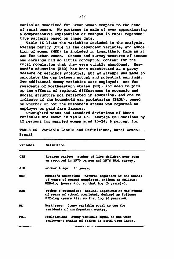
137

variables deacribed for urban W08en compare to the caaeof rural women. No pretenae ia made of even approximatinga comprehenaive explanation of changea in rural reproduc­tive patterns baaed on theae data.

Table 46 lists the variables included in the analysis.Average parity (CEB) is the dependent variable, and educa­tion of W08en (MID) is included in logarithaic form as itwas for urban W08en. Cenaua and aurvey meaaures of incomeand earninga had ao little conceptual content for therural population that they were quickly abandoned. Bua­band'a education (BED) haa been aubatituted aa a proxymeaaure of earninga potential, but no atte~t was made tocalculate the gap between actual and potential earninga.Two additional du..y variablea were e~loyedl one forreaidenta of Northeaatern statea (NB), included to pickup the effecta of regional differencea in economic andsocial atructure not reflected in education, and one toindicate if the household was proletarian (PROL), baaedon whether or not the huaband' a atatua waa reported aae~loyee or paid farm laborer.

Unweighted meana and atandard deviationa of thesevariablea are ahewn in Table 47. Average CEB declined by12 percent for married W08en aged 20-24, 6 percent for

TABLE 46 Variable Labels and Definitions, Rural WOIDenaBrazil

Variable Definition

CBB Average parity. nUllber of live children ever born.. reporteeS in 1970 cenaua and 1976 PIIAD auney.

AGE

RED

PRJL

Mother 'a age. in yeara.

Mother'a education. natural logaritlul of the nUllberof yeara of achool coapleted, defined aa followa.MBD-log (yeara +1), 80 that log (0 yeara) -0.

Pather 'a education. natural logaritlul of the nUllberof yeara of achool coapleted, defined .. followa.RIm-log (yeara +1), ao that log (0 yeara) -0.

Northe..t, d~ variable equal to one forreaidenta of northeutern atatea.

Proletar ian. d~ var iable equal to one whenellpl~nt autua of father ia rural wage labor.

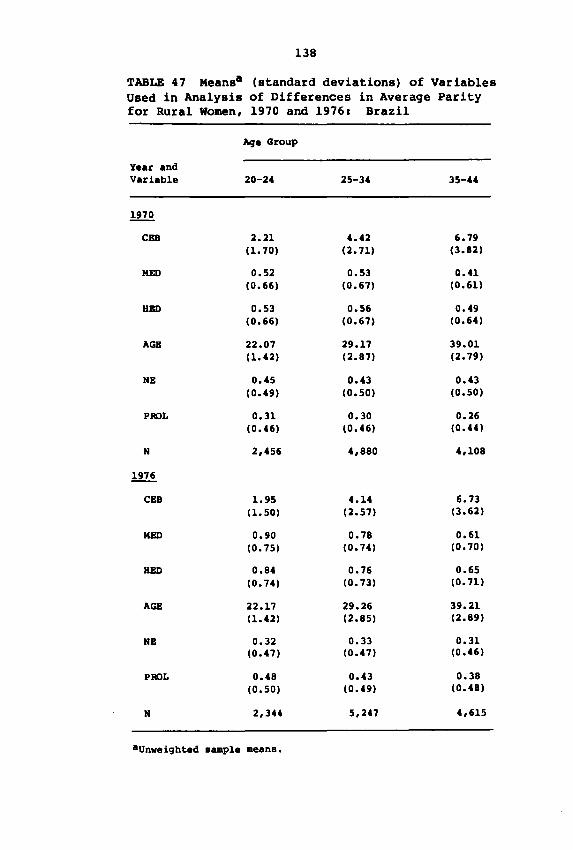
138

TABLE 47 Meansa (standard deviations) of VariablesUsed in Analysis of Differences in Average Parityfor Rural Women, 1970 and 1976: Brazil

A/Je Group

Year andVariable 20-24 25-34 35-44

1970

CBB 2.21 4.42 6.79(1.70) (2.71) (3.82)

MED 0.52 0.53 0.41(0.66) (0.67) (0.61)

HED 0.53 0.56 0.49(0.66) (0.67) (0.64)

AGE 22.07 29.17 39.01(1.42) (2.87) (2.79)

NE 0.45 0.43 0.43(0.49) (0.50) (0.50)

PROL 0.31 0.30 0.26(0.46) (0.46) (0.44)

N 2,456 4,880 4,108

ill.!

CBB 1.95 4.14 6.73(1.50) (2.57) (3.62)

MED 0.90 0.78 0.61(0.75) (0.74) (0.70)

HED 0.84 0.76 0.65(0.74) (0.73) (0.71)

AGE 22.17 29.26 39.21(1.42) (2.85) (2.89)

NE 0.32 0.33 0.31(0.47) (0.47) (0.46)

PROL 0.48 0.43 0.38(0.50) (0.49) (0.48)

N 2,344 5,247 4,615

aUnweighted sllDlp1e means.

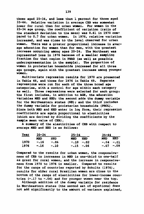
139

those aged 25-34, and leaa than 1 percent for those aged35-44. Relative variation in average CEB was aomewhatlower for rural than for urban women. For women in the25-34 age group, the coefficient of variation (ratio ofthe standard deviation to the mean) was 0.61 in 1970 com­pared to 0.7 for urban women. In 1976, relative variationincreased, and waa cloae to the level obaerved for urbanwomen. There was a greater proportional increase in aver­age education for women than for men, with the greatestincreaae occurring &DOng ages 20-24. The Northeaat waarepreaented leaa in 1976 becauae of a -.aller aaaplingfraction for that region in PNAD (aa well aa poaaibleunderrepresentation in the aample). The proportion ofwomen in proletarian houaeholda increaaed for all threeage groups, again with the greateat increaae among youngerwomen.

Multivariate regreaaion resulta for 1970 are presentedin Table 48, and those for 1976 in Table 49. Separateregreasiona were run for each of the three broad agecategoriea, with a control for age within each categoryas well. Three regreaaiona were aelected for each group:the firat includea, in addition to AGE, the educationvariablea MBD and BED, the second adds the du..y variablefor the Northeastern atates (HB), and the third includesthe dummy variable for proletarian houaeholda (PReL).Since both MBD and BED enter in log form, their regressioncoefficients are again proportional to elaaticitiea(which are derived by dividing the coefficients by thesaaple mean value of CEB).

A summary of the elasticitiea of CEB with reapect toaverage MBD and BED is as follows:

19701976

20-24MBD-.16-.16

BED-.06-.10

25-34MBD BED-.10 -.02-.15 -.06

35-44MBD BED-.04 -.01-.07 -.08

Compared to the results for urban women, the responsive­ness of CBB to increases in MBD is one-third to one-halfas great for rural women, and the increase in responsive­ness from 1970 to 1976 is smaller. Compared to resultsfor the range of countries reported by Schultz (1976),results for older rural Brazilian women are close to thebottom of the range of elasticities for lower-income coun­tries (-.17 to -.04) and for younger women near the top.

Although addition of the dummy variable for residencein Northeastern states (the second set of equations) doesnot add significantly to the amount of variance explained,

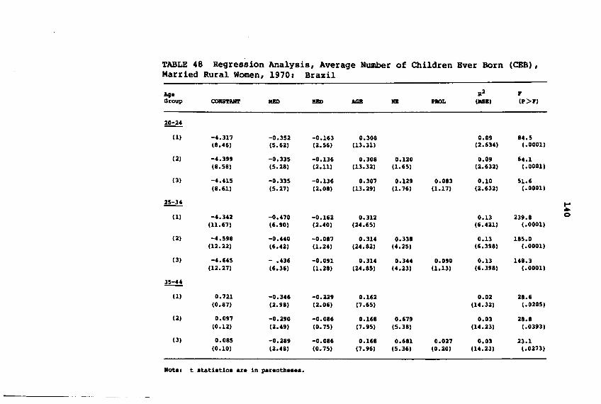
TABLE 48 Regression Analysis, Average Humber of Children Ever Born (CBS) ,Married Rural Women, 1970: Brazil

Ag. R2 PGroup COIIS'1'AIft' MBI) BED AGB lIB PIlOL (IISB) (P>P)

~

(1) -4.317 -0.352 -0.163 0.308 0.09 84.5(8.46) (5.62) (2.56) (13.31) (2.634) (.0001)

(2) -4.399 -0.335 -0.136 0.308 0.120 0.09 64.1(8.58) (5.28) (2.11) (13.32) (1.65) (2.632) (.000l)

(3) -4.415 -0.335 -0.136 0.307 0.129 0.083 0.10 51.6(8.61) (5.27) (2.08) (13.29) (1.76) (1.17) (2.632) (.0001)

~ ......(1) -4.342 -0.470 -0.162 0.312 0.13 239.8 0

(11.67) (6.90) (2.40) (24.65) (6.421) (.000l)

(2) -4.598 -0.440 -0.087 0.314 0.338 0.13 185.0(12.22) (6.42) (1.24) (24.82) (4.25) (6.398) (.000l)

(3) -4.645 - .436 -0.091 0.314 0.344 0.090 0.13 148.3(12.27) (6.36) (1.28) (24.85) (4.23) (1.13) (6.398) (.0001)

ll=!!(1) 0.721 -0.346 -0.229 0.162 0.02 28.6

(0.87) (2.98) (2.06) (7.65) (14.32) (.0205)

(2) 0.097 -0.290 -0.086 0.168 0.679 0.03 28.8(0.12) (2.49) (0.75) (7.95) (5.38) (14.23) (.0393)

(3) 0.085 -0.289 -0.086 0.168 0.681 0.027 0.03 23.1(0.10) (2.48) (0.75) (7.96) (5.36) (0.20) (14.23) (.0273)

Rote I t .tati.tic. are in par.nth•••••

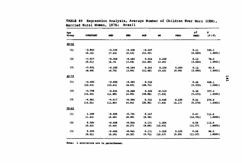
TABLE 49 Regression Analysis, Average Humber of Children Ever Born (CEB) ,

Married Rural Women, 1976: Brazil

Ag. a2 PGroup COIIS'1'AIft' IIIID DD AGII lIB .... OISB) IP>P)

~

(1) -2.803 -0.339 -0.238 -0.237 O.ll 100.316.10) 17.22) 15.03) Ill.49) 12.009) 1.000l)

(2) -3.0l7 -0.ll8 -0.194 0.242 0.235 0.12 78.516.5l) 16.78 13.94) Ill.69) 13.45) 12.000) 1.0001)

(3) -3.021 -0.320 -0.194 0.241 0.236 0.005 0.12 62.816.49) 16.78) 13.94) Ill.6I) 13.42) 10.08) (2.000) 1.0001)

~ ......(1) -4.495 -0.650 -0.362 0.322 0.20 428.1

....Ill. 55) 112.42) 16.85) 128.72) 15.325) 1.0001)

(2) -4.768 -0.621 -0.261 0.322 -0.519 0.20 337.2114.34) Ill.88) 14.95) 128.89) 17.22) 15.273) 1.0001)

(3) -4.861 -0.6l7 -0.266 0.323 0.540 0.140 0.21 270.9114.51) Ill.80) 14.91) 128.96) 17.44) 12.17) 15.270) 1.0001)

~

(1) 1.009 -0.555 -0.7ll 0.167 0.07 lll.611.43) 16.40) 18.48) (9.36) 112.251) 1.000l)

(2) 0.304 -0.468 -0.546 0.17l 1.204 0.09 112.910.43) 15.44) 16.27) (9.69) 110.43) Ill.97) 1.000l)

(3) 0.222 -0.462 -0.541 0.17l 1.219 0.105 0.09 90.510.ll) 15.36) 16.20) 19.72) 110.47) 10.99) Ill.97) 1.0001)

IIote. t .tati.tic. are in par.ntbe....

142

the regression coefficient is significant for the twoolder age groups. This indicates an interaction betweeneducation and residence rather than an additive effect.Tests for the interaction suggested that MED slopes werelower in the Northeast, though so few rural women in thatregion reported any education that it was difficult tojudge the significance of the results.

The third set of equations attempted to assess theimpact of proletarianization on average CEB. The resultswere consistent with the tabular results in Chapter 3,which suggested that CEB was slightly higher in proletar­ian rural households. When other variables were con­trolled, however, this difference was significant onlyfor women in the 25-34 age group in 1976. These resultsconfirm the point made earlier that an adequate test ofthe proletarian hypothesis will require a more precisemeasurement of the process of proletarianization thatcaptures present and previous residence and occupationalstatus, as well as a richer depiction of the institutionalforces underlying that process.

Changes in Rural CEB from 1970 to 1976

The change in average CEB from 1970 to 1976 that can beaccounted for in the regression analysis results fromincreased educational attainment. In this connection, itshould be recognized that most of the observed change isnot explained by changes in the variables included in theregressions. It is hoped that the case study datareported in Part II of this report will provide richerinsight into the nature of changes in rural fertilitythan do aggregate census and sample survey data.

CONCLUSIONS

Most of the variance in average parity that can beexplained by application of multivariate regression anal­ysis to data on individual married women from the Brazil­ian census and PNAD survey relates to modernizationvariables--education and average earnings. Most of thechange that can be accounted for between 1970 and 1976relates to increases in these two variables. The attemptto incorporate a variable measuring the relative economicposition of urban households indicated that there was apositive association between fertility and relative eco-

143

nomic status, that is, CEB was higher on average for womenwhose husbands' current earnings exceeded the level ofearnings that would be expected given their education andother characteristics. However, decomposition of changesin CBB from 1970 to 1976 did not show that a change in GAPcontributed to fertility decline.

These regressio~ results do not suggest that increasedmodernization was the only reason for the change in Bra­zilian fertility. Changes in regression coefficients andin constant terms in the regression equations suggestedthat a variety of unmeasured factors could account for theunexplained variance. Measures that were available in thecensus and survey data provided little insight into thenature of such changes, whether related to increasedaccess to contraception through public or private chan­nels, or to institutional changes associated with shiftsin the Brazilian model of socioeconomic development.

It should also be recognized that average parity is apoor measure of fertility for purposes of accounting forchange. It is a cumulative variable, and comparisons ofaverages for different groups at different dates measurethe result of a demographic process rather than the pro­cess itself. As noted above, it would have been betterto use current fertility as measured by births reportedfor the year prior to the interview, however, as reportedin Chapter 2, the performance of that measure inspiredmore confidence in its robustness for work with subgroupsof the population. Attempts to derive other measures(such as the length of the first open birth interval) fromthese data files proved equally unrewarding.

Data limitations curtailed even further the analysisof differences and the decomposition of changes in theaverage parity of rural women. The main finding for thesewomen was that increased educational attainment contri­buted most to the explanation of variance, though only alimited portion of the total variance was explained by theregressions. some doubts were raised about the hypothesisthat proletarianization contributed to fertility decline,however, caution was suggested about the validity of usingdata on rural women classed as proletarian at the time ofthe interview to test this hypothesis, rather than usingthe experience of the proletarianization process.

It was also impossible to link what the census and sur­vey data reported about the demographic characteristicsof individual rural residents and their families to eco­nomic characteristics of their farms and institutionalfeatures of their localities. For this reason, the study

144

could not explore hypotheses relating fertility declineto changes in land availability, reduced need for childlabor, and increased nonfarm economic activity for ruralwomen and children. The census and survey data files didinclude questions on school attendance that merited fur­ther study. Information on child labor was included inagricultural censuses, but not in the demographic censusesand surveys. If Brazil is ever to conduct a fertilitysurvey patterned after the World Fertility Survey, itwould focus ideally on these elements of rural socioeco­nomic structure, as well as those aspects of change inurban areas that are not covered by currently availablecensus and survey data.

PART II FERTILITY OE'l'BRMIHAHTS AT TBB LOCAL LEVEL

CHAPTER 5

TBB NID: PURPOSB AND MBTBODOLOGY

AS noted in the Introduction, the diacu••ion in this andthe following chapter. parallels Part I, but with alocal- rather than a national-level focu.. There are, ofcourse, advantages to be gained from both: the national­level analysis permits aggregate conclusions andhypotheses, however tentative, the local-level dataexamined in the following pages provides another,complementary per.pective on tho.e perceptions. Thesechapters examine the purpose and methodology of the NID,levels and trends in the total fertility rate for thenine local contexts studied, and the effects of nup­tiality, marital fertility patterns, the proxi-atedeterminants, and socioeconomic factors, specificallyincome, on fertility for the nine context.. The finalchapter shows that the national-level and the local-levelconclusions are consistent.

The NID was conducted between May 1975 and March 1977by Centro Basileiro de Analise e Planejamento (CEBRAP) inSao Paulo, under the financial auspices of the Inter­national Development Research Centre (lORe, Canada), thePopulation Council (USA), and Pinanciadora de Estudos eProjectos (PINEP, Brazil). It consists of a series oflocal case studies based on a view of population dynamicsas part of the overall structural dynamics of society,with economic determinants (manpower requirements, formsand degrees of accumulation, property patterns, etc.)having a decisive influence. However, this dominance ofsocioeconomic factors over population dynamics does notoperate in an obvious way. Therefore, rather than simplyassuming such relations, it is essential to examineanalytically and empirically how they are established.Although structures condition behavior, and behavior onlyexists through the actions of individuals (with their

145

146

aspirations, motivations, forms of personality, indi­vidually calculated interests, etc.), the mediationbetween structures and action is essential. If themediations are not taken into account, the analysis mustinevitably become static. The result is the deduction ofrigid prescriptions for action from structural patterns,or, at the opposite extreme, the dissolution of socialconditioning factors into the SUbjectivity of theindividual agents, so that the only way to understandhuman reproduction is to take a purely psychologicalapproach. The NIHR perspective takes the role of socialinstitutions--the Church, private enterprise, theeducational system, the medical system, and so on--asbeing crucial to such mediation. The way populationpractices and values are actually realized, andpopulation policies defined, depends on how population isseen in the context of these institutions, and how,within each one, interests and values concerning thefamily, number of children, procreation, and familyplanning are articulated.

The NIHR began by choosing the areas of Brazil thatwould represent as purely as possible the different formsin which the production is organized. A two-dimensionaltypology of the areas was then developed according totheir dominant forms of production and their place in theprocess of development. 2 In the former category, threemodes were distinguished, each of which might predominatein a given area, although in combination with the others:the capitalist mode, a system of small autonomous pro­ducers, and rural servitude. The capitalist form wassubdivided into monopolistic and competitive, for thesmall autonomous producers, the distinction was betweenrural and urban. The second dimension, place in the pro­cess of development, was based on the assumption thatdevelopment tends to concentrate economic activities andpopulation in certain areas, and to disperse them inothers. The former were classed as ·concentration areas,·which are invariably urban, the latter were labeled ·dis­persion areas,· which as a rule comprise extractive oragriCUltural activities, with the formation of frontiersat the edges of an overexpanding transportation system.This classification also left room for certain areas,labeled ·interstitial,· which fall between the types des­cribed above, and which tend to lose activities and popu­lation, these areas may be either urban or rural.

These two dimensions could produce a total of 15 pos­sible types. However, four of these were discarded as

147

meaningless: the monopolistic and interstitial capitalistarea, simple commodity production with an urban locationin a dispersion area, simple. commodity production with arural location in a concentration area, and rural servi­tude in a concentration area. The monopolistic capitalistarea undergoing dispersion was also discarded since it wasconsidered highly rare in its pure state in Brazil, more­over, within a given gradient, it might appear in someregions classified as competitive-capitalist in a dis­persed form. Finally, rural servitude in an interstitialform was also omitted since this combination might befound, at least partially, in regions defined as simplecommodity production with a rural location and intersti­tial form.

The next stage of analysis consisted of making thenine remaining possibilities correspond to actual regionsin Brazil. Regions were distributed both spatially and,whenever possible, according to the dual classification.The results are shown in Table 50, the contexts selectedare described in detail in the Appendix. The nine areaschosen cover seven municipalities (for the sake ofconvenience, the rural and urban categories in the sys­tem of autonomous producers are represented by the ruraland urban areas of the same municipalities, thus yieldingnine area types and only seven municipalities). Thesemunicipalities are distributed over six states: SaoPaulo, Rio Grande do Sul, Pernambuco, Espirito Santo,Para, and Piaui. The map of Brazil (see page 14) givesan idea of this geographical distribution.

For each of the nine chosen areas, two types of studywere performed: a macro-structural study covering thewhole population of the area, and following this, a surveybased on a probabilistic sample of the population in thesame area.

The aim of the macro-structural study was to acquireas complete as possible a knowledge of the dynamics of thepopulation, its socioeconomic structure, and the area'ssocial institutions from its foundation to the present.The three components of population dynamics consideredwere natality, mortality, and migration. The socioeco­nomic factors considered essential to the study's objec­tives were the area's landowning structure, product mix,and predominant types of activity, the number of personsengaged in work and the types of occupations (present andprevious), the duration and type of land occupation, pro­duction values and forms of appropriation of surplus, andproduction techniques. The study of institutions focused

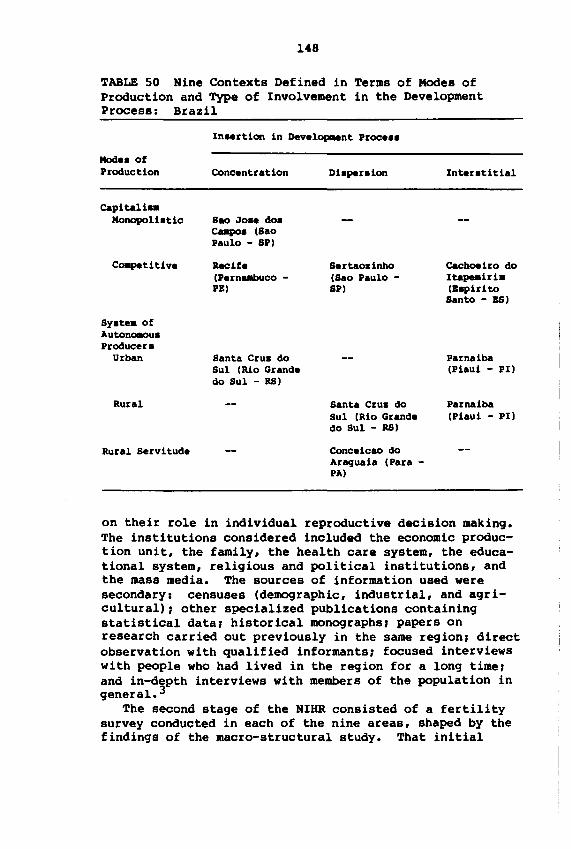
148

TABLE 50 Nine Contexts Defined in Terms of Modes ofProduction and Type of Involvement in the DevelopmentProcess: Brazil

In..rtion in Devel~nt Proce••

Mode. ofProduction

c&pitalbaMonopolbtic

Coapetitive

Sy.tea ofAutonClllOu.Producer.

Urban

Rural

Rural Servitude

Concentr.tion

SIlO Jo.. do.CuIpo. (SaoPaulo - SP)

Recife(Pernaabuco ­PB)

Santa Crus doSul (Rio Grandedo Sul - RB)

Dbpenion

Sertaodnho(Sao Paulo ­SP)

Santa Crus doSul (Rio Grandedo Sul - RB)

Conceicao doAraguaia (Para ­PAl

Intentiti81

C&choeiro doI tapeairia(BapiritoSanto - 88)

Parnaiba(Piaui - PI)

Parnaiba(Piaut - PI)

on their role in individual reproductive decision making.The institutions considered included the economic produc­tion unit, the family, the health care system, the educa­tional system, religious and political institutions, andthe mass media. The sources of information used weresecondary: censuses (demographic, industrial, and agri­cultural)J other specialized pUblications containingstatistical dataJ historical monographsJ papers onresearch carried out previously in the same regionJ directobservation with qualified informantsJ focused interviewswith people who had lived in the region for a long timeJand in-depth interviews with members of the population ingeneral. 3

The second stage of the NIHR consisted of a fertilitysurvey conducted in each of the nine areas, shaped by thefindings of the macro-structural study. That initial

149

study helped delineate the sample by revealing, forexample, the production relations prevailing in the areaJthe rural proletariat and its spatial distribution, bothin the countryside and on the urban outskirts of a munici­palitYJ the annual cycle of each region's range of majorproducts, coupled with the rainy and dry seasonsJ and theseasonality of harvests requiring harvest workers. In­depth interviews a-ong the population in general wereanother i~rtant aid in designing the survey. The sam­pling procedure proposed for the survey was three-stageequiprobabilitYI the priaary sampling unit was a censustract, the secondary unit a block, and the tertiary unita household. Whenever possible, appropriate samplingfractions were determined to ensure that each householdin a given region had the same probability of belongingto the sample.

A household was understood as a group of people linkedby kinship, affinity, or econoaic relations and livingunder the same roof. Bach was given a questionnaire con­sisting of three modules.

The first, known as the household module, containedinformation on all the meabers of the household, identify­ing them through their relation to the head of the house­hold, as well as their age, sex, marital status, level ofschooling, occupation (type of activity, position, andperiodicity), monthly earnings, and consumption. Inaddition, there was information on help given to orreceived from other members of the group not living in thehousehold, and on the division of labor within it. Inrural areas, additional questions concerned the differentarrangements for land tenure, types of harvest, number ofaniaals, agricultural implements, and the like. Duringthe interview, this information was given by any adultconsidered a qualified informant and a meaber of thehousehold group.

The second module, a life history, was designed toobtain fundamental quantitative data for a study of repro­duction strategies. Unlike most fertility studies, theNIRR was not limited t~ women between ages lS and 49 instable marital unions. Any member of the householdgroup was eligible for this module, as well as for thethird, described below. S Some clarification is requiredconcerning the inclusion of males in this survey.Although rarely carried out in practice, the need for thisinclusion has been pointed to with some frequency in theliterature since the husband's role in decision makingwithin the family, his position on the use of contracep-

150

tives, and so ~n are important determinants of reproduc­tive behavior. In the NIBR, inclusion of males isjustified not only for these reasons, but also for othersreSUlting from the theoretical approach adopted: sincethe NIBR set out to link the forms of production to modesof reproduction, the agent most closely linked with theproduction process was eSPeCially important. One indivi­dual was selected at random from each household forapplication of the life history module and referred tothereafter as the Ego. The Ego's life history was fol­lowed from birth to the present. Information was gatheredon migration, education, and occupation, as well as on thecomposition of and changes in the Ego's family group. Themodule also contained a detailed reproductive history,beginning with the menarche (for women) or earliest sexualrelation (for men) and continuing up to the menopause orandropause, respectively, with information gathered onunions, duration and result of pregnancies, use of con­traceptives, breastfeeding, surviving children, dates ofdeath of nonsurvivors, and so on. If the Ego then hadprevious or current marital unions, the life history ofthe spouse was gathered in equal detail from the beginningof the union. Information given by Ego was also used toreconstruct, in less detail, the spouse's life history atthree points prior to the union--at birth, age 10, andage 18.

Finally, the third module, also answered by the Ego,was aimed at obtaining transversal material to explain anumber of actual practices involving the relationshipbetween institutions and reproductive behavior. Theseincluded the existence of distinct plans or strategiesregarding reproduction, help given to and received fromchildren, and the like.

In conclusion, it should be emphasized that the NIHRwas not intended as a representative national sample. Itssamples are representative only in relation to the areaor municipality from which they were selected. Given thecharacteristics of the study, it would be practicallymeaningless to aggregate the nine contexts to provideestimates of national-level demographic parameters. Thusthe discussion that follows, while parallel to that ofPart I in many ways, is quite different in focus, andserves as a complement to that analysis.

CBAP'l'BR 6

THE 'l'OTAL FERTILITY BATRI LBVBLS AND TRENDS

aefore proceeding with an analy.i. of the total fertilityrate ba.ed on NIBR data, it i. worth clarifying aa-epoints with regard to the.e data. The NIBR .urvey. wereperforaed with the aia of covering 400 hou.ehold. in eacharea except Sao Jose dos Campo. and Recife, where 800households per area were included. As mentioned above,the information unit wa. any adult. However, for purposesof the following analysi., the unit will be taken as aWCllllall, and SOIIle cc:..ents should be aade in this con­nection.

Fir.t, it is worth noting that the information on awoman's reproductive history (contained in the life­history module) was given by the woman when she wa. theselected adult, or by her mate when he was selected,whether his wife was alive or not. Thus, the samples donot refer only to cohorts of women who survived until thesurvey, and it is not neces.ary to make the usual assump­tion that the fertility experience of women who did notsurvive is faithfully represented by the experience ofthose who did. With this in mind, whenever the reproduc­tive history of an adult is considered, the woman may havebeen in anyone of the following situationsl

1. alive and single2. alive and married3. alive and separated4. alive and widowed5. dead and married while alive

Situations 1, 3, and 4 could only occur if the woman wasthe informant, situation 5 could only occur if a man wasthe informant, and situation 2 could occur in either case.

Second, the fact that the investigation also includedsingle women avoided the problem of completeness involved

151

152

in leaving out all childbearing experienced by women whodeclared they were single at the time of the survey. Atthe same time, it meant that, in general, the premaritalexperience of women ever married at the time of the surveywas not eliminated.

Third, it ahould be stressed that in this investigationthere was no cut-off age for asking questions on fertilityhistory. Thus the data were not truncated, as usuallyhappens when histories are not obtained for women overage SO. This means that fertility rates could be cal­culated for almost all age groups and for a distant past,although it must be remembered that memory problems mayintroduce certain difficulties.

The total fertility rates (Table 51) were establiahedfor three different points in timea 1965, 1970, and 1975.For each of theae periods, the rates were calculated onthe basis of the total number of women alive at that time,regardless of marital status. Thus if a woman was alive,for instance, in 1965, she was not necessarily alive in1970 or after. Moreover, when the informant (Ego) was ahusband separated from his wife during the year for whichthe fertility rate was calculated, this case was elimi­nated, since there was no way of knowing that woman'ssituation with regard to the number of children betweenthe year of separation and the year of reference for cal­culating fertility. A further clarification is requiredconcerning the dates of the surveys. For seven out ofthe nine areas, the surveys were conducted in 1976 or1977, thus, the data for births in 1975 present no prob­lems as to the calendar year. However, in Sao Jose dosCampos, the survey was performed from May to December1975, and in Santa Cruz do Sul-Urban from November 1975to July 1976. A correction was thus necessary for thesetwo areas since the women in both were not exposed for thewhole year. For Sao Jose dos Campos, the number of birthsin 1975 was multiplied by the factor 1.530, and for SantaCruz do Sul-Urban by 1.045.

The first observation to be made when analyzing Table51 is that there is some consistency between these resultsand those of Table 2 from Part I of this report. Indeed,the 1970 rate for Sao Jose (4.83) was consistent with thatfor Sao Paulo State (4.07), especially given that morethan 70 percent of the latter's population was urban in1970. Similarly, for Parnaiba-Rural, Parnaiba-Urban, andRecife, located in Northeast Brazil, total fertility asreported in Table 51 varied from 8.42 to 5.45 in 1970, theTable 2 value for the Northeast (7.58) is within this

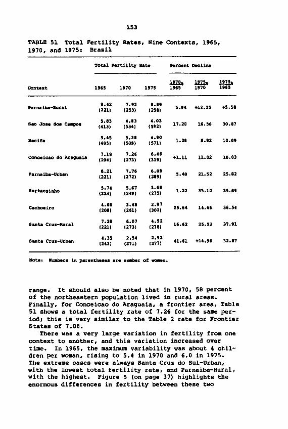
153

TABLE 51 Total Fertility Rates, Nine COntexts, 1965,1970, and 19751 Brazil

'fota1 rertility Rate Percent Decline

!m.t !12h !UhCOntext l!t65 1910 l!t75 U65 U70 U65

Parnaiba-Rural8.42 7.n 8.89

5." +12.25 +5.58(2211 (2531 (2581

SIlO Jo.. de» CuIloa 5.83 ~.83 ~.0317.20 16.56 30.87

(~131 (53~1 (5UI

Recife 5.U 5.38 ~.90 1.28 8.92 10.09(~051 (5091 (5711

Conce1cao do ArAfjuaia 7.18 7.26 6.U+1.11 11.02 10.03

(20~1 (2731 (3191

Parnaiba-Urban 8.21 7.76 6.095.U 21.52 25.82(2211 (2721 (2891

Sutaodnho 5.7~ 5.67 3.681.22 35.10 35.89

(22~1 (2~91 (2751

caeboeiro ~.68 3.48 2.9725.U U.66 36.5~(2081 (2611 (3021

Santa Crux-Rural 7.28 6.07 ~.5216.62 25.53 37.91(2211 (2731 (2781

Santa Crux-Urban~.35 2.5~ 2.U n.n +U.96 32.87(2UI (2711 (2771

Hotel .~r. 1n parentbe... are n~r of wa.en.

range. It should also be noted that in 1970, 58 percentof the northeastern population lived in rural areas.Finally, for COnceicao do Araguaia, a frontier area, Table51 shows a total fertility rate of 7.26 for the same per­iod, this is very similar to the Table 2 rate for FrontierStates of 7.08.

There was a very large variation in fertility from onecontext to another, and this variation increased overtime. In 1965, the maximum variability was about 4 chil­dren per woman, rising to 5.4 in 1970 and 6.0 in 1975.The extreme cases were always Santa Cruz do Sul-Urban,with the lowest total fertility rate, and Parnaiba-Rural,with the highest. Figure 5 (on page 37) highlights theenormous differences in fertility between these two

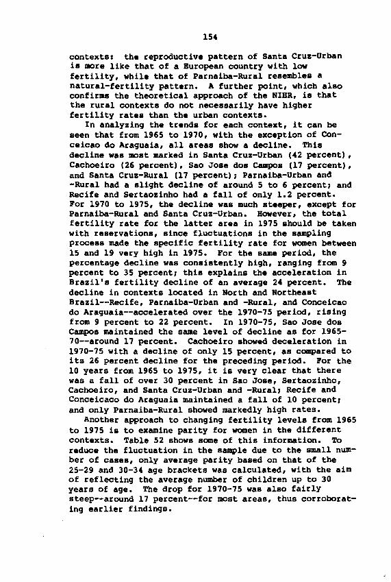
154

contexts I the reproductive pattern of Santa Cruz-Urbanis more like that of a European country with lowfertility, while that of Parnaiba-Rural resembles anatural-fertility pattern. A further point, which alsoconfirms the theoretical approach of the NIBR, is thatthe rural contexts do not necessarily have higherfertility rates than the urban contexts.

In analyzing the trends for each context, it can beseen that from 1965 to 1970, with the exception of Con­ceicao do Araguaia, all areas show a decline. Thisdecline was most marked in Santa Cruz-Urban (42 percent) ,Cachoeiro (26 percent), Sao Jose dos campos (17 percent),and Santa Cruz-Rural (17 percent)J Parnaiba-Urban and-Rural had a slight decline of around 5 to 6 percentJ andRecife and Sertaozinho had a fall of only 1.2 percent.For 1970 to 1975, the decline was much steeper, except forParnaiba-Rural and Santa Cruz-Urban. However, the totalfertility rate for the latter area in 1975 should be takenwith reservations, since fluctuations in the samplingprocess made the specific fertility rate for women between15 and 19 very high in 1975. For the same period, thepercentage decline was consistently high, ranging from 9percent to 35 percentJ this explains the acceleration inBrazil's fertility decline of an average 24 percent. Thedecline in contexts located in North and NortheastBrazil--Recife, Parnaiba-Urban and -Rural, and Conceicaodo Araguaia--accelerated over the 1970-75 period, risingfrom 9 percent to 22 percent. In 1970-75, Sao Jose dosCampos maintained the same level of decline as for 1965­70--around 17 percent. Cachoeiro showed deceleration in1970-75 with a decline of only 15 percent, as compared toits 26 percent decline for the preceding period. For the10 years from 1965 to 1975, it is very clear that therewas a fall of over 30 percent in Sao Jose, Sertaozinho,Cachoeiro, and Santa Cruz-Urban and -RuralJ Recife andConceicaco do Araguaia maintained a fall of 10 percentJand only Parnaiba-Rural showed markedly high rates.

Another approach to changing fertility levels from 1965to 1975 is to examine parity for women in the differentcontexts. Table 52 shows some of this information. Toreduce the fluctuation in the sample due to the small num­ber of cases, only average parity based on that of the25-29 and 30-34 age brackets was calculated, with the aimof reflecting the average number of children up to 30years of age. The drop for 1970-75 was also fairlysteep--around 17 percent--for most areas, thus corroborat­ing earlier findings.

155

TABLE 52 Mean Parity 1/2 (P25-29 + P30-34)' 1965, 1970,and 19751 Brazil

1970, 1975,Context 1965 1970 1975 1965 1970

Santa Crus-Orban 2.32 1.99 1.65 14.22 17.08

Santa Crus-Rural 2.92 3.16 2.80 +8.22 11.39

Cachoeiro 2.99 2.57 2.09 14.05 18.68

Sao Jose dos Caapos 3.13 3.02 2.48 3.51 17.88

Recife 3.27 3.09 2.72 5.50 11.97

Sertaodnho 3.54 3.41 2.91 1.98 16.14

Conceicao do Araguaia 3.93 4.25 4.34 +8.14 +2.12

Parnaiba-Orban 4.44 4.33 3.58 2.48 17.32

Parnaiba-Rural 4.68 4.70 4.42 +0.43 5.96

The central que.tion posed by the data reported aboveis why contexts with very different social and economicstructures show such similar rates of decline, while morestailar context••how such different rate.. The discu.­sion that follows explores this que.tion by examining therole of nuptiality and marital fertility in the fertilitydeclines observed at the local level (Chapters 7 and 8)7the role of the proximate determinants (Chapter 9)J andthe role of socioeconomic factors, SPeCificallyfamily income (Chapter 10).

CHAPTER 7

NUPTIALITY

As will be seen in the next chapter, a decline in maritalfertility was the primary determinant of the fertilitydeclines noted above. This conclusion parallels that ofthe national-level analysis in Part I. Before analyzingmarital fertility, however, it is important to examinesome other determinants related to nuptiality--the typeof union and the initial, mean, and final age at mar­riage--that can contribute to a rise or fall in fertility.

TYPE OF UNION

Distribution of Types of Union

Table 53 shows the distribution of ever-married women fromthe NIHR according to tyPe of union in three periods oftime--1960, 1970, and 1975. Before this table is anal­yzed, some points must be made about the various tyPes ofunion. During the colonial and imperial periods in Bra­zil, marriages were performed by the Catholic Church. In1890, however, civil marriage was legally instituted asthe only valid form of marriage. Since then, those whofollow some kind of religion have continued to conductreligious marriages, either exclusively or as a complementto legal marriage. Two other tyPes of union are presentin Brazilian society: consensual union and permanentunion. Both of these are also known as free unions sincethey are not limited by any tyPe of binding connection,civil or religious. Both consensual and permanent unionsare defined as stable: in the former, the couple live inthe same housei in the latter, they do not.

Comparing the nine NIHR contexts (Table 53), for afixed time period, say 1975, there is a great difference

156

157

in the types of union, ranging from the situation in whichpractically all union. were legal (Santa Cruz do Sul­Urban) to the opposite extreme, in which less than 30percent of couples legalized their unions (Parnaiba­Rural). It is also noteworthy, in the same line ofthought, that in Parnaiba-Urban and -Rural, and in Con­ceicao do Araguaia, the category Religious Only accountedfor a large number of unions, in the other contexts, freeunion was more common than religious union, even reachingone-third of all unions in Recife. This diversity a-ongcontexts found for 1975 can al.o be seen for earlier per­iods from at least 1960 onward, as the data in Table 53clearly show. Indeed, in 1960 the proportion of legalunions varied from 29.9 percent in Parnaiba-Rural to 92.5percent in Santa Cruz-Urban, between these extremes, therewere intermediate figures such as 52.0 percent inParnaiba-Urban, 63 percent in Araguaia, and 66.6 percentin Recife. What is noteworthy here, however, is that forall contexts, the main change over the 15 years analyzedconsisted of a gradual decline in religious as comparedwith free unions. In certain contexts, this decline wassmaller, as in Sao Jose and Santa Cruz-UrbanJ in othersit was greater, as in Parnaiba-Urban and -Rural, and inRecife. In Sertaozinho, the fall in the number of relig­ious union. was not sufficient to account for the increasefound for free union., but was partly due to a reductionin the relative weight of legal unionsJ the same can besaid of Conceicao do Araguaia.

This relative increase in free unions as a result of afall in either religious or legalized unions is also shownin Table 54, based on the findings of the 1960 and 1970censuses and the 1978 PNAD (National Household SampleSurvey). It should be observed that in these sources,free unions include only consensual unionsJ there is noexplicit mention of permanent unions. From this it canbe concluded that the latter have been incorporated ineither the consensual or single category. Indeed, the1970 census defined single women as follows: -those womenwho have not entered into any civil or religious, or civiland religious marriage, and do not live in a stable con­sensual union.-

The data in Table 54 also lend some validity to thefindings from the NIHR shown in Table 53 (which are depen­dent on sample fluctuations given the small number ofcases): there is a great deal of similarity between thecontexts (Table 53) within a partiCUlar region and theresults for that same region (Table 54)J in other words,

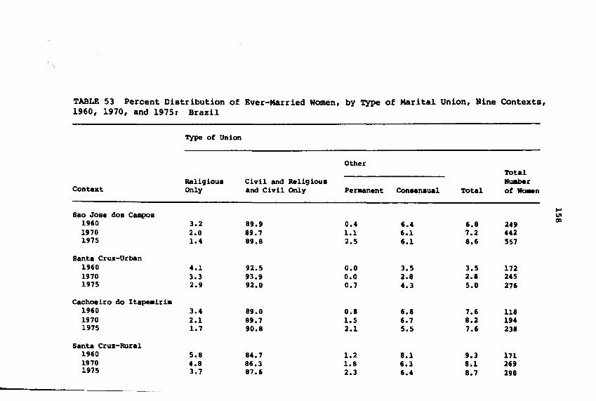
TABLE 53 Percent Distribution of Ever-Married Women, by Type of Marital Union, Nine Contexts,1960, 1970, and 1975: Brazil

Type of Union

OtherTotal

Religious Civil and Religious IIU11berContext Only and Civil Only Peraanent Consensual Total of~n

....Sao JOBe dos Campos U!

1960 3.2 89.9 0.4 6.4 6.8 249 CD

1910 2.0 89.7 1.1 6.1 7.2 4421975 1.4 89.8 2.5 6.1 8.6 557

Santa Cruz-Urban1960 4.1 92.5 0.0 3.5 3.5 1721970 3.3 n.g 0.0 2.8 2.8 2451975 2.9 92.0 0.7 4.3 5.0 276

Cachoelro do Ita~lrim

1960 3.4 89.0 0.8 6.8 7.6 1181910 2.1 89.7 1.5 6.7 8.2 1941975 1.7 90.8 2.1 5.5 7.6 238

Santa Cruz-Rural1960 5.8 84.7 1.2 8.1 9.3 1711970 4.8 86.3 1.8 6.3 8.1 2691975 3.7 87.6 2.3 6.4 8.7 298

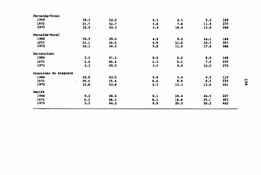
Parnaiba-Urban1960 39.2 52.0 4.1 4.1 8.2 1691970 35.7 52.7 3.8 7.6 11.4 2351975 32.8 53.3 3.4 10.4 13.8 268

Parnaiba-Rural1960 55.9 29.9 4.9 9.2 14.1 1841970 55.1 28.5 4.9 11.0 16.3 2631975 52.1 30.0 5.9 11.9 17.8 286

Sertaolinbo1960 3.0 91.1 0.0 6.0 6.0 1681970 2.2 90.4 1.3 6.1 7.4 2301975 2.2 85.5 3.0 g.O 12.0 270

Conceicao do Araguaia1960 32.8 63.0 0.8 3.4 4.2 1191970 35.0 55.4 0.4 8.9 9.3 234 ...

Ul1975 32.6 53.8 0.3 13.3 13.6 301 ID

Recife1960 9.2 66.6 6.1 18.4 24.5 2271970 6.3 68.3 8.3 16.8 25.1 3631975 5.2 64.2 g.g 20.3 30.2 462

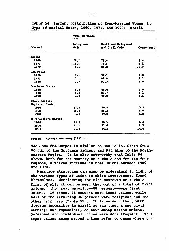
160

TABLE 54 Percent Distribution of Ever-Married Women, byType of Marital Union, 1960, 1970, and 19781 Brazil

Type of Union

..1191011. Civ11 and ..li91011.Conteat Only and Civil only Co~n.ua1

81'••111960 20.2 73.4 6.41'70 14.4 78.6 8.11978 8.1 81.2 10.7

Bao ••u101960 5.1 92.1 2.81970 3.1 92.8 4.11978 1.7 90.3 8.0

Southern State.1960 9.6 16.8 3.61'70 6.2 89.7 4.11978 3.5 90.0 6.5

Kina. Gerai./Bapil'1to Santo

1960 17.9 78.9 3.21970 10.8 85.2 4.01978 5.0 89.0 6.4

Harthe••tern State.1960 42.5 48.1 9.41970 33.1 57.6 9.31978 21.5 64.1 14.4

SOurces AIt8ann and WOII9 (U8lbl.

Sao Jose d08 Campos is similar to Sao Paulo, Santa Cruzdo Sul to the Southern Region, and Parnaiba to the North­eastern Region. It is also noteworthy that Table 54shows, both for the country as a whole and for the fourregions, a marked increase in free unions between 1960and 1978.

Marriage strategies can also be understood in light ofthe various types of union in which interviewees foundthemselves. Considering the nine contexts as a wholefirst 0; all, it can be seen that out of a total of 2,234unions, the great majority--88 percent--were firstunions. Of these, 71 percent were legal unions, whilehalf of the remaining 30 percent were religious and theother half free (Table 55). It is evident that, withdivorce impossible in Brazil at the time, a new civilmarriage was impossible, so that among second unions,permanent and consensual unions were more frequent. Thuslegal unions among second unions refer to cases where the

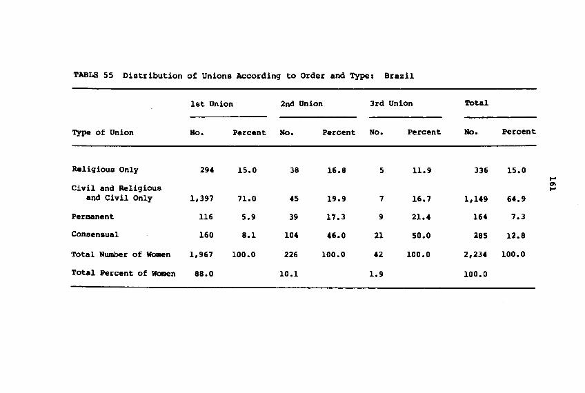
TABLE 55 Distribution of Unions According to Order and Type: Brazil

1st Union 2nd Union 3rd Union Total

Type of Union No. Percent No. Percent No. Percent No. Percent

Relig ious Only 294 15.0 38 16.8 5 11.9 336 15.0 ...Civil and Religious 01...

and Civil Only 1,397 71.0 45 19.9 7 16.7 1,149 64.9

Permanent 116 5.9 39 17.3 9 21.4 164 7.3

Consensual 160 8.1 104 46.0 21 50.0 285 12.8

Total Number of Women 1,967 100.0 226 100.0 42 100.0 2,234 100.0

Total Percent of Women 88.0 10.1 1.9 100.0

162

first legal union ended in widowhood, or the first relig­ious or free union ended in separation.

It is immediately noteworthy that at the start of theirmarried lives, 14 percent of women (or of men or of part­ners) preferred no binding connection, and 6 percent didnot even choose the bond of living together. This typeof preference is a focal point of the discussion in thepresent chapter. First, the chapter analyzes whether thiskind of behavior is more common in more recent than inolder unions. Next, it examines whether even the conven­tional rural/urban distinction differentiates this behav­ior. Finally, these issues will be elaborated by exaain­ing each context individually.

Table 56 shows the distribution of the total of 1967first unions of ever-married women according to when theunion occurred, that is, women married by 1960, between1961 and 1970, and after 1970. As can be seen, more thanhalf were older unions--before 1960--while 29.1 percenttook place between 1961 and 1970, the rest were morerecent unions. It is interesting to note that the prefer­ence for legal unions remained at the same level: about71 percent of first unions were legal, irrespective ofwhen they were initiated. Religious unions, however,gradually lost their relative position, falling from 18.4percent for older unions to 7.3 percent for those initi­ated after 1970, there was also a concomitant rise in per­manent and consensual unions, which together accountedfor 21.3 percent of more recent unions. In other words,the points made in the analysis of Tables 53 and 54 aresupported by using as a reference point whether the unionis recent or not, that is, the different marriage cohorts.

A breakdown of the total sample from the nine contextsinto urban and rural shows first that within both groupsthere is considerable similarity in the temporality offirst unions. Indeed, 52 percent and 51 percent of womenwere married before 1960 in urban and rural contexts,respectively, for both contexts 29 percent were marriedbetween 1961 and 1970. On the other hand, some veryinteresting differences can be seen in both contexts inregard to types of unions and timing. As regards thepreference for religious union as the first union, inurban contexts, this preference declined drastically overtime, from 14.0 percent to 2.6 percent, a drop of 5.4times (see Table 57), in the rural areas, the drop wasonly 1.8 times. For more recent rural marriages, religi­ous unions represented about the same proportion (13.8percent) as that for marriages that took place at least

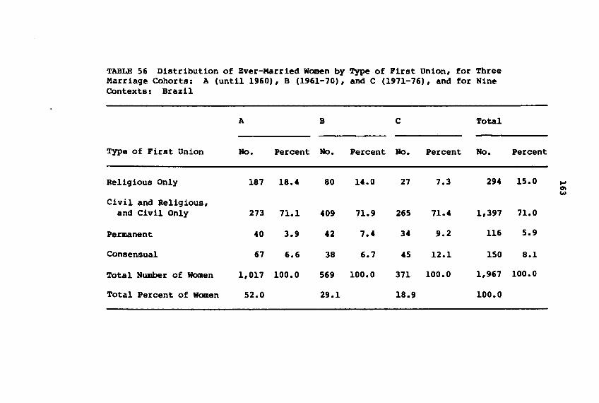
TABLE 56 Distribution of Ever-Married Women by Type of First Union, for ThreeMarriage Cohorts: A (until 1960), B (1961-70), and C (1971-76), and for NineContexts: Brazil

A B C Total

-Type of First Union No. Percent No. Percent No. Percent No. Percent

Religious Only 187 18.4 80 14.0 27 7.3 294 15.0 ....01w

Civil and Religious,and Civil Only 273 71.1 409 71.9 265 71.4 1,397 71.0

Permanent 40 3.9 42 7.4 34 9.2 116 5.9

Consensual 67 6.6 38 6.7 45 12.1 150 8.1

Total Number of WOmen 1,017 100.0 569 100.0 371 100.0 1,967 100.0

Total Percent of Women 52.0 29.1 18.9 100.0

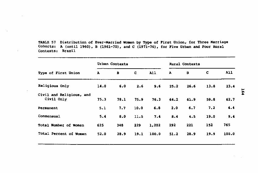
TABLE 57 Distribution of Ever-Married Women by Type of First Union, for Three MarriageCohorts: A (until 1960), B (1961-70), and C (1971-76), for Five Urban and Four RuralContexts: Brazil

Urban Contexts Rural Contexts

Type of First Union A B C All A B C All

--Religious Only 14.0 6.0 2.6 9.6 25.2 26.6 13.8 23.4 ....

0\Civil and Religious, and ..

Civil Only 75.3 78.1 75.9 76.3 64.2 61.9 59.8 62.7

Permanent 5.1 7.7 10.0 6.8 2.0 6.7 7.2 4.4

Consensual 5.4 8.0 11.5 7.4 8.4 4.5 19.0 9.4

Total Number of Women 625 348 229 1,202 292 221 152 765

Total Percent of Women 52.0 28.9 19.1 100.0 51.2 28.9 19.9 100.0

165

15 years ago in urban contexts (14.0 percent). Moreover,in the rural contexts, the preference for legal unionsalso fell in relative terms, although less drastically.At the same time, there was a moderate rise (and a steeperone than in the urban contexts) in permanent and consen­sual unions as a percentage of all first unions, thisreached 26.2 percent of initial preferences for morerecent unions.

The next step in the analysis was to investigate howthese findings operated within each context, that is, tosee how the preferences for the various types of unionamong the total first unions developed over time. To thisend, Table 58 shows the distribution of ever-married womenaccording to the type of union, for the same three marri­age cohorts. It may be noted immediately that in all con­texts, there was a progressive increase in permanent andconsensual unions, only Santa Cruz-Urban showed any sta­bilization in the proportions of permanent unions, whileonly in Cachoeiro did consensual unions show an increasein proportions, followed by a decrease.

In this comparison of contexts, it is highly interest­ing to note that in the country's poorer areas analyzedhere--Parnaiba and COnceicao do Araguaia--religiousunions represented a noteworthy alternative among unionsoccurring before 1960, indeed, they competed with legalunions in Parnaiba-Urban and overtook them in Parnaiba­Rural. A number of different reasons may explain this.First, work relations, above all in the countryside, thenoffered no protection in the form of social security forindividuals or their families, thus no documents wererequired on family structure, birth of children, and soon. Another reason, somewhat related to the first, maybe the fact that no property was owned that could bedivided for inheritance. It is also worth mentioning thepossible absence of civil registries at that time in cer­tain areas of the country, whereas churches have alwaysbeen universally present. Then, too, the continuation ofthe custom of religious marriage, which is so deep-seatedin Northeast Brazil, represented a resistance to the newrelative prominence granted the Catholic Church by theRepublic. Finally, religious marriage as a first unioncan be seen as a forerunner of legalized union.

The relative decline of religious unions in these con­texts may be due to changes in all or some of these ele­ments. One change is undeniable: access to registriesbecame easier with improved communications. Moreover, thefact that a legalized union entitled one to social secur-

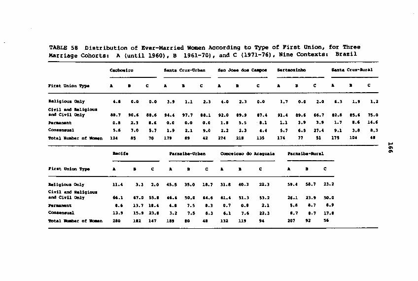
TABLE 58 Distribution of Ever-Married Women According to Type of First Union, for ThreeMarriage Cohorts: A (until 1960), B 1961-70), and C (1971-76), Nine Contexts: Brazil

Cacboeiro Sanu Crua-Urban Sao JON doa ca.po. SerUOainbo Sanu Crua-aural

---Firat Union Type A 8 C A 8 C A 8 C A 8 C A 8 C

.aUgioua Only 4.1 0.0 0.0 3.' 1.1 2.3 4.0 2.3 0.0 1.7 0.0 2.0 6.3 1.' 1.2

Ciyil and aaligiouaand Civil Only 11.7 '0.6 11.6 94.4 97.7 ".1 92.0 It., 87.4 91.4 1t.6 66.7 82.1 15.6 75.0

Pa~nant 0.1 2.3 1.6 0.0 0.0 0.0 1.1 5.5 1.1 1.1 3.' 3.' 1.7 1.6 14.6

Coneanaual 5.6 7.0 5.7 1.' 2.1 '.0 2.2 2.3 4.4 5.7 6.5 27.4 '.1 3.1 1.3

'1'otal MUllbar of --'n 124 15 70 17' It U 274 211 135 174 77 51 175 104 U ...0\

Recifa .arnaiba-Urban eonceicao do Araguaia .arnaiba-aural 0\

Firat Union Type A 8 C A 8 C A 8 C A 8 C

aaUgioua Only 11.4 3.3 2.0 45.5 35.0 11.7 31.1 40.3 22.3 59.4 58.7 23.2

Ciyil and aaligiouaand Ciyil Only 66.1 67.0 55.1 46.6 50.0 64.6 61.4 51.3 53.2 26.1 23.' SO.O

Pa~nt 1.6 13.7 11.4 4.1 7.5 1.3 0.7 0.1 2.1 5.1 1.7 I.'Conaenaual 13.' 15.' 23.1 3.2 7.5 1.3 6.1 7.6 22.3 1.7 1.7 17.1

'1'oUl ....r of --'n 210 112 147 11' 10 U 132 11' 94 207 92 56

167

ity certainly represented a stimulus. For example, inParnaiba, the Social Security Office performs a mostimportant role in the life of wage-earners (Loyola, 1978),many of whom are laid off for sickness due to nervousexhaustion. They then register with the Social SecurityOffice and, as they themselves put it, -stay on the shelf­for months or even years receiving benefits. A new supplyof labor is therefore recruited to replace those laid off.When some of these fresh workers are in turn laid offsick, some who have previously been laid off are reem­ployed, and 80 on. Thus, each family group always has thepossibility of one of its members being either laid offand receiving a portion of his or her wage from the gov­ernment, or employed and receiving the full wage.Although this situation may seem strange, it representsan attempt to overcome the problem of poverty in theregion, or to -redistribute poverty.-

At the other extreme low proportions of religiousunions are observed in most contexts, except unions initi­ated before 1960 in Recife, where this type of union stillrepresented 11 percent of the total (Table 58). In Cach­oeiro and Sao Jose dos Campos, this proportion was alreadylow, falling to zero for more recent unions.

As for legal unions, Cachoeiro practically maintaineda stable pattern (around 90 percent), Santa Cruz-Urban and-Rural, which accounted for the highest level of legalunions, saw an increase of this type of union from thefirst to the second cohort, mainly because of a drop inthe relative importance of religious unions. In these twocontexts, the decline in the relative weight of legalunions among more recent unions can be explained directlyby an increase in free unions. It should be rememberedthat Santa Cruz do Sul is made up largely of Europeanimmigrants, mostly of German origin, who developed family­based agricultural activities and later SPeCialized intobacco growing. This led the urban part of the munici­pality to develop an industrial complex based on the pro­cessing of tobacco. The prominance of legal unions canbe linked not only to cultural factors, but also to issuesof property ownership and inheritance. One possibleexplanation of any decline in the proportion of legalunions may therefore be removal of the latter stimulus bythe breaking up of these properties, already small, overthe years. In Sao Jose dos Campos, where much of theworking population is employed on a wage-earning basis bylarge and medium-sized companies, it could only beeXPeCted that legalized unions would account for a highpercentage of the total number of unions.

168

The Role of Consensual Unions

To understand Brazilian marriage strategies, it is eSsen­tial to examine the role of consensual unions more close­ly. Consensual union may be an option for living togetherwhen there is no stiaulus for legalized union, as discus­sed above. To this reason should be added the far fromnegligible cost of a civil marriage. 8 In Parnaiba, forexample, one can clearly observe the phenomenon of -mar­riage by seduction- (Loyola, 1978) as a strategy to avoidspending money on a civil, or even a religious, marriage.This represents a method used by women--above all thosefrom the poorer groups within the population--to guaranteea union in a context where the male-female ratio in the15-49 age group was only 841100 in 1960 and 1970. Oncethe girl had been -seduced,- her family summoned the-seducer- and demanded that he remain with the girl -tocorrect his error,- but without a dowry or any weddingfeasts or ceremonies, as a pseudo-punishment.

Consensual unions are also a solution to separationsfollowing lf9al or even religious unions. Indeed, upuntil 1978, dissolutions of legal unions, even whenformalized before a judge (desquite), made new civilunions impossible. The Catholic Church also does not per­mit a second religious union, since this bond is indis­soluble according to the law of God. Thus, the only wayto marry again was through a free union.

Consensual union may also result from a change invalues that sees legal bonds as unnecessary. This may beespecially important among the younger groups of the pop­ulation, as part of a general questioning of traditionalnorms and values. Women's liberation has made women bothmore economically independent and more disposed to expresstheir sexuality, again leading to a preference for freeunions.

The preference for consensual union may reflect adefinitive decision, or it may represent a preliminarystage in conjugal life prior to a legal and/or religiousunion. It is also probable that pregnancy may contributeto legalization in large Brazilian metropolises. However,the size of the cities included in the NIBR, such asRecife and Sao Jose dos Campos, together with the timecovered by the survey (which stopped at 1977), made itimpossible to support this conclusion empirically.

The issue raised here can be clarified by a brief anal­ysis of,'consensual unions for each of the nine contexts.To this end, the following classification has been devel­oped:

169

(1) consensual union as the only union(2) consensual union following a legal union(3) consensual union following a religious union(4) consensual union prior to a legal union(5) consensual union prior to a religious or permanent

union

The study was made based on the three above-mentionedmarriage cohorts, with results as shown in Table 59.

It should be noted at the start that the small numberof cases for each context, except Recife, permits a .erelyillustrative analysis of each situation. It must also beremembered that marriage strategies are a dynamic processJthus a woman living in a consensual union at a givenmoment has a certain probability of legalizing it or ofentering a religious union at any subsequent moment.

Sao Jose dos Campos is one context where the greatmajority of consensual unions represented a second orthird union following a civil marriage. It thus illus­trates situations (2) and (3). Out of the total of 42cases, 16 occurred before 1960, a further 16 between 1961and 1970, and the remaining 10 after 1970. For older con­sensual unions, 68.7 percent occurred as the only marriagesolution after a legal union. This proportion fell to56.3 percent for the following cohort, while for morerecent unions it was 60.0 percent. The 6 cases out of 42in which consensual union preceded a civil union tookplace before 1971. Of these, 3 cases involved the legal­ization of a consensual union, with 2 cases taking placeafter the birth of a childJ in the other 3 cases, thelegal union was with a different person. Situation (1)represented 9 cases, or 21.4 percent of the totalJ these9 cases were equally distributed over the three marriagecohorts.

Parnaiba-Rural illustrates a certain balance betweenthe types of consensual unions, with the greatest inci­dence for situations (4) and (5) (34.5 percent). As notedabove, religious union has always been highly valued inthis region, one of Brazil's poorest. Thus there were 6cases in which a consensual union preceded a legal unionand 13 in which it preceded a religious union. Of these6 former cases, 5 were unions legalized with the same per­son, with 3 of these occurring after the birth of chil­dren. Of the 13 cases where religious unions followedconsensual unions, 50 percent were with the same person,with the bearing of children an associated factor. InParnaiba-Rural, it is also worth noting that 21 of the 55

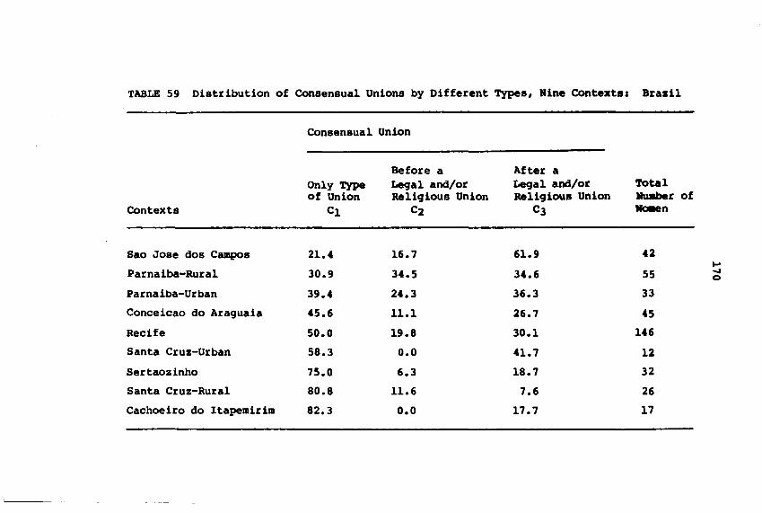
TABLE 59 Distribution of Consensual Unions by Different Types, Rine Contextsl Brasil

Consensual Union

Before a After aOnly Type Legal and/or Legal and/or Totalof Union Religious Union Religious Union Hwlber of

Contexts Cl C2 C3 woaen

Sao Jose dos Campos 21.4 16.7 61.9 U....

Parnaiba-Rural 30.9 34.5 34.6 55 ....0

Parnaiba-Urban 39.4 24.3 36.3 33

Conceicao do Araguaia 45.6 11.1 26.7 45

Recife 50.0 19.8 30.1 146

Santa Cruz-Urban 58.3 0.0 41.7 12

Sertaozinho 75.0 6.3 18.7 32

Santa Cruz-Rural 80.8 11.6 7.6 26

Cachoeiro do Itapemirim 82.3 0.0 17.7 17

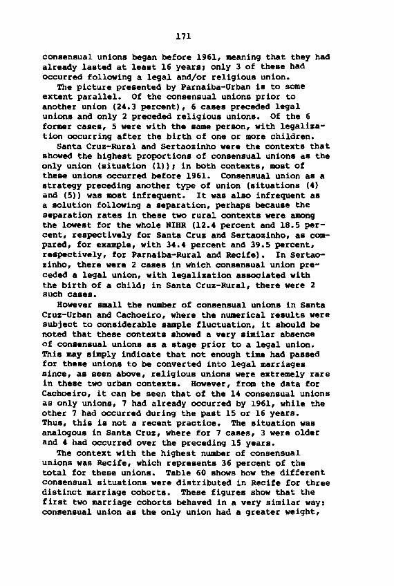
171

consensual unions began before 1961, meaning that they hadalready lasted at least 16 years, only 3 of these hadoccurred following a legal and/or religious union.

The picture presented by Parnaiba-Urban is to someextent parallel. Of the consensual unions prior toanother union (24.3 percent), 6 cases preceded legalunions and only 2 preceded religious unions. Of the 6former cases, 5 were with the same person, with legaliza­tion occurring after the birth of one or more children.

Santa Cruz-Rural and Sertaozinho were the contexts thatshowed the highest proportions of consensual unions as theonly union (situation (1», in both contexts, most ofthese unions occurred before 1961. Consensual union as astrategy preceding another type of union (situations (4)and (5» was most infrequent. It was also infrequent asa solution following a separation, perhaps because theseparation rates in these two rural contexts were amongthe lowest for the whol. NIHR (12.4 percent and 18.5 per­cent, respectively for Santa Cruz and Sertaozinho, as com­pared, for example, with 34.4 percent and 39.5 percent,respectively, for Parnaiba-Rural and Recife). In Sertao­zinho, there were 2 cases in which consensual union pre­ceded a legal union, with legalization associated withthe birth of a child, in Santa Cruz-Rural, there were 2such cases.

However small the number of consensual unions in SantaCruz-Urban and Cachoeiro, where the numerical results weresUbject to considerable sample fluctuation, it should benoted that these contexts showed a very similar absenceof consensual unions as a stage prior to a legal union.This may simply indicate that not enough time had passedfor these unions to be converted into legal marriagessince, as seen above, religious unions were extremely rarein these two urban contexts. However, from the data forCachoeiro, it can be seen that of the 14 consensual unionsas only unions, 7 had already occurred by 1961, while theother 7 had occurred during the past 15 or 16 years.Thus, this is not a recent practice. The situation wasanalogous in Santa Cruz, where for 7 cases, 3 were olderand 4 had occurred over the preceding 15 years.

The context with the highest number of consensualunions was Recife, which represents 36 percent of thetotal for these unions. Table 60 shows how the differentconsensual situations were distributed in Recife for threedistinct marriage cohorts. These figures show that thefirst two marriage cohorts behaved in a very similar waysconsensual union as the only union had a greater weight,

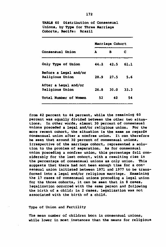
172

TABLE 60 Distribution of ConsensualUnions, by Type for Three MarriageCohorts, Recifes Brazil

Marriage Cohort

Consensual Union A B C

Only Type of Union 44.2 42.5 61.1

Before a Legal and/orReligious Union 28.9 27.5 5.6

After a Legal and/orReligious Union 26.8 30.0 33.3

Total Number of Waaen 52 40 54

from 42 percent to 44 percent, while the remaining 60percent was equally divided between the other two situa­tions. In other words, almost 30 percent of consensualunions preceded a legal and/or religious union. Por themore recent cohort, the situation is the same as regardsconsensual union after a nonfree union. It can thereforebe seen that around 30 percent of consensual unions,irrespective of the marriage cohort, represented a solu­tion to the problem of separation. As for consensualunion preceding a nonfree union, this percentage fell con­siderably for the last cohort, with a resulting rise inthe percentage of consensual unions as only union. Thissuggests that there had not been enough time for a con­sensual union initiated between 1971 and 1977 to be trans­formed into a legal and/or religious marriage. Examiningthe 17 cases of consensual unions preceding a legal unionfor the three cohorts, it can be seen that in 8 cases,legalization occurred with the same person and followingthe birth of a child, in 2 cases, legalization was notassociated with the birth of a child.

Type of Union and Pertility

The mean number of children born in consensual unions,while lower in most instances than the means for religious

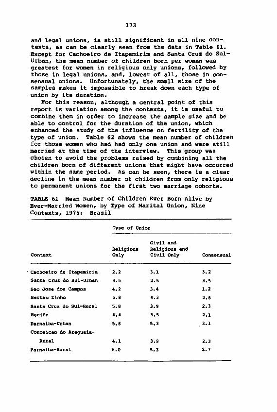
173

and legal unions, is still significant in all nine con­texts, as can be clearly seen from the data in Table 61.Except for Cachoeiro de Itapemirim and Santa Cruz do Sul­Urban, the mean number of children born per woman wasgreatest for women in religious only unions, followed bythose in legal unions, and, lowest of all, those in con­sensual unions. Unfortunately, the small size of thesamples makes it impossible to break down each type ofunion by its duration.

For this reason, although a central point of thisreport is variation among the contexts, it is useful tocombine them in order to increase the sample size and beable to control for the duration of the union, whichenhanced the study of the influence on fertility of thetype of union. Table 62 shows the mean number of childrenfor those women who had had only one union and were stillmarried at the time of the interview. This group waschosen to avoid the problems raised by combining all thechildren born of different unions that might have occurredwithin the same period. As can be seen, there is a cleardecline in the mean number of children from only religiousto permanent unions for the first two marriage cohorts.

TABLE 61 Mean Number of Children Ever Born Alive byEver-Married Women, by Type of Marital Union, NineContexts, 1975: Brazil

Type of Union

Civil andReligious Religious and

Context Only Civil Only COnsensual

. Cachoeiro de Itapemirim 2.2 3.1 3.2

Santa Cruz do Sul-Urban 3.5 2.5 3.5

Sao Jose dos C.-pos 4.2 3.4 1.2

Sertao Zinho 5.8 4.3 2.6

Santa Cruz do Sul-Rural 5.8 3.9 2.3

Recife 4.4 3.5 2.1

Parnaiba-Urban 5.6 5.3 3.1

Conceicao do Araguaia-

Rural 4.1 3.9 2.3

Parnaiba-Rural 6.0 5.3 2.7

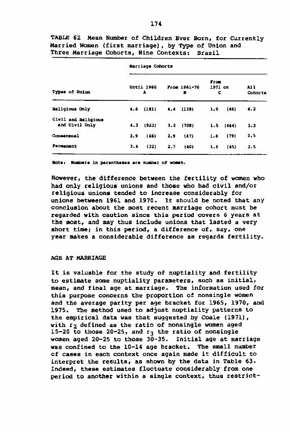
174

TABLE 62 Mean Number of Children Ever Born, for CurrentlyMarried Women (first marriage), by Type of Union andThree Marriage Cohorts, Nine Contexts: Brazil

Marriag. Cohort.

FroaUntil 1960 Froa 1961-70 1971 on All

Type. of Union A B C Cohorts

1Ie11giou. Only 4.6 (181) 4.4 (128) 1.9 (46) 4.2

Civil and 1Ie1igiou.and Civil Only 4.3 (922) 3.2 (708) 1.5 (464) 3.3

eon..n.ua1 3.9 (46) 2.9 (47) 1.6 (79) 2.5

P.~nt 3.4 (32) 2.7 (40) 1.6 (45) 2.5

Ilot.1 BWlber. in par.nth.... are nWlber of ~n.

However, the difference between the fertility of women whohad only religious unions and those who had civil and/orreligious unions tended to increase considerably forunions between 1961 and 1970. It should be noted that anyconclusion about the most recent marriage cohort must beregarded with caution since this period covers 6 years atthe most, and may thus include unions that lasted a veryshort time, in this period, a difference of, say, oneyear makes a considerable difference as regards fertility.

AGE AT MARRIAGE

It is valuable for the study of nuptiality and fertilityto estimate some nuptiality parameters, such as initial,mean, and final age at marriage. The information used forthis purpose concerns the proportion of nonsingle womenand the average parity per age bracket for 1965, 1970, and1975. The method used to adjust nuptiality patterns tothe empirical data was that suggested by Coale (1971),with r2 defined as the ratio of nonsingle women aged15-20 to those 20-25, and r3 the ratio of nonsinglewomen aged 20-25 to those 30-35. Initial age at marriagewas confined to the 10-14 age bracket. The small numberof cases in each context once again made it difficult tointerpret the results, as shown by the data in Table 63.Indeed, these estimates fluctuate considerably· from oneperiod to another within a single context; thus restrict-

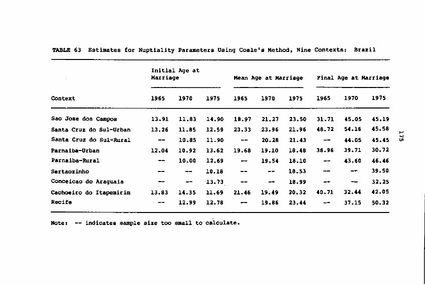
TABLE 63 Estimates for Nuptia1ity Parameters Using Coale's Method, Nine Contexts: Brazil

--Initial Age atMarriage Mean Age at Marriage Final Age at Marriage

-Context 1965 1970 1975 1965 1970 1975 1965 1970 1975

Sao Jose dos Campos 13.91 11.83 14.90 18.97 21.27 23.50 31.71 45.05 45.19

Santa Cruz do Su1-Urban 13.26 11.85 12.59 23.33 23.96 21.96 48.72 54.16 45.58I-'

Santa Cruz do Su1-Rura1-.I-- 10.85 11.90 -- 20.28 21.43 -- 44.05 45.45 UI

Parnaiba-Urban 12.04 10.92 13.62 19.68 19.10 18.48 38.96 39.71 30.72

Parnaiba-Rural -- 10.00 12.69 -- 19.54 18.10 -- 43.60 46.46

Sertaozinho -- -- 10.18 -- -- 18.53 -- -- 39.50

Conceicao do Araguaia -- -- 13.73 -- -- 18.99 -- -- 32.25

Cachoeiro do Itapemirim 13.83 14.35 11.69 21.46 19.49 20.32 40.71 32.44 42.05

Recife -- 12.99 12.78 -- 19.86 23.44 -- 37.15 50.32

Note: -- indicates sample size too small to calculate.

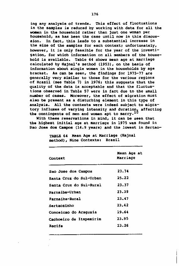
176

ing any analysis of trends. This effect of fluctuationsin the samples is reduced by working with data for all thewomen in the household rather than just one woman perhousehold, as has been the case until now in this discus­sion. In fact, this leads to a substantial increase inthe size of the samples for each context, unfortunately,however, it is only feasible for the year of the investi­gation, for which information on all members of the house­hold is available. Table 64 shows mean age at marriagecalculated by Hajnal's method (1953), on the basis ofinformation about single women in the households by agebracket. As can be seen, the findings for 1975-77 aregenerally very similar to those for the various regionsof Brazil (see Table 7) in 1976, this suggests that thequality of the data is acceptable and that the fluctua­tions observed in Table 57 were in fact due to the smallnumber of cases. Moreover, the effect of migration mustalso be present as a disturbing element in this type ofanalysis. All the contexts were indeed subject to migra­tory influxes of varying intensity and duration6 affectingthe contingents of men and women apt to marry.l

With these reservations in mind, it can be seen thatthe highest initial age at marriage in 1975 was found inSao Jose dos Campos (14.9 years) and the lowest in Sertao-

TABLE 64 Mean Age at Marriage (Hajnalmethod), Nine Contextsl Brazil

Mean Age atCOntext Marriage

Sao Jose dos Campos 23.74

Santa Cruz do Sul-Urban 25.22

Santa Cruz do Sul-Rural 23.37

Parnaiba-Urban 23.39

Parnaiba-Rural 23.47

Sertaozinho 23.42

Conceicao do Araguaia 19.64

Cachoeiro de Itapemirim 23.95

Recife 23.26

177

zinho (10.2 years). These extremes seem consistent withthe mean for Brazil in 1976, estimated by Altmann and Wong(198lb), at 13.3 years. For the Northeastern region, theage found was 12.7 years, very close to the values forRecife (12.8) and Parnaiba-Rural (12.7). For 1970-75,even taking all the above reservations into account, itcan be seen that, in general, there was a certain increasein the initial age at marriage. As regards the final llgeat marriage, an important index of nuptiality and closelyrelated to the -marriage market,- the larger urban centersand metropolises were the regions that most favored latemarriager this applies to Recife, Sao Jose dos Campos, andSanta Cruz do Sul-Urban, contexts in which final ages werehighest in 1975. With some exceptions, it can also besaid that the final age at marriage generally increasedbetween 1970 and 1976.

It should be observed, on the other hand, that thecontingent of women who remain single after a given agedepends, among other things, on the availability of men-exposed to the risk- of forming a union. In 1970, thesex ratio varied considerably in the 15-49 age bracket forall the areas studied. If the information at the levelof municipalities from the 1970 census is used, the sexratios per 1,000 women aged 15-49 were as followsl Ser­taozinho, 1,115, Sao Jose, 1,040, Santa Cruz, 970, Cacho­eiro, 960, Parnaiba, 953, Recife, 785. The proportionsof women still single in the 30-39 age bracket, as shownby the data at the household level, were, in the sameorder, as follows: 7.4 percent, 8.8 percent, 9.1 percent,12.3 percent, 12.5 percent, and 14.8 percent. In otherwords, the higher the sex ratio, the lower the proportionof still single women.

Given the reservations mentioned above, it may be con­cluded from this descriptive analysis that, despite thedifferent levels in the parameters for the various con­texts, initial age at marriage is rising, mean age atmarriage is also increasing, and final age at marriage hasalso risen. What is far less clear from these data is thetiming of the changes, which makes it difficult to drawfirm conclusions about how they affect fertility levels.In any case, as indicated in the following chapters, theprimary factor involved in Brazil's accelerated fertilitydecline is declining marital fertility, traceable tochanging patterns of contraceptive use.

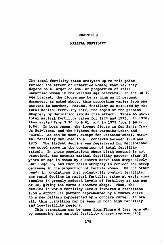
CHAPTER 8

MARITAL FERTILITY

The total fertility rates analyzed up to this pointreflect the effect of unmarried women, that is, theydepend on a larger or smaller proportion of still­unmarried women in the various age brackets. In the 30-39age bracket, the figure may be as high as 15 percent.Moreover, as noted above, this proportion varies from onecontext to another. Marital fertility as measured by thetotal marital fertility rate, the topic of the presentchapter, by definition avoids this effect. Table 65 showstotal marital fertility rates for 1970 and 1975. In 1970,they varied from 3.70 to 9.61, and in 1975 from 2.96 to9.64. In both cases, the lowest figure is for Santa Cruzdo Sul-Urban, and the highest for Parnaiba-Urban and-Rural. As can be seen, except for Parnaiba-Rural, mari­tal fertility declined in all contexts between 1970 and1975. The largest decline was registered for Sertaozinho(as noted above in the comparison of total fertilityrates). In those populations where birth control is notpracticed, the natural marital fertility pattern after 25years of age is shown by a convex curve that drops slowlyuntil age 35, and then falls abruptly to reflect the steepdecrease in the proportion of fertile women. On the otherhand, in populations that voluntarily control fertility,the rapid decline in marital fertility rates at early agesresults in greatly reduced levels of fertility at the ageof 30, giving the curve a concave shape. Thus, thedecline in world fertility levels involves a transitionfrom a structural pattern represented by a convex curveto a new pattern represented by a concave curve. In Bra­zil, this transition can be seen in both high-fertilityand low-fertility regions.

This transition can be seen from Figure 6 (see page 40)by comparing the marital fertility curves representing

178

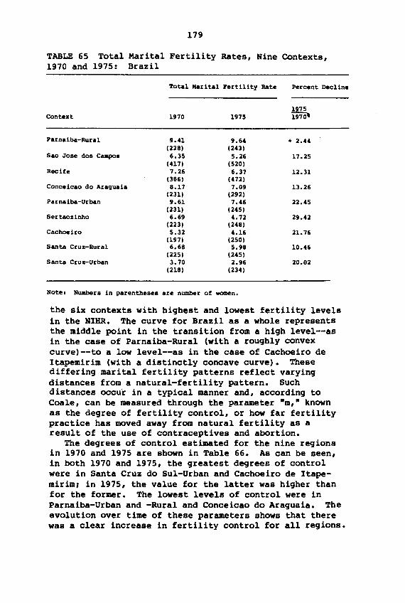
179

TABLE 65 Total Marital Fertility Rates, Nine Contexts,1970 and 1975: Brazil

Total Marital Fertility Rate Percent Decline

1975Context 1970 1975 1970'

Parnaiba-Rural 9.41 9.64 + 2.44(228) (243)

Sao Jose dos Campos 6.35 5.26 17.25(417) (520)

Recife 7.26 6.37 12.31(386) (472)

Coneeieao do Araguaia 8.17 7.09 13.26(231) (292)

Parnaiba-Urban 9.61 7.46 22.45(231) (245)

Sertaozinho 6.69 4.72 29.42(223) (248)

Caehoeiro 5.32 4.16 21.76(197) (250)

Santa Cruz-Rural 6.68 5.98 10.46(225) (245)

Santa Cruz-Urban 3.70 2.96 20.02(218) (234)

Note. Numbers in parentheses are number of women.

the six contexts with highest and lowest fertility levelsin the NIHR. The curve for Brazil as a whole representsthe middle point in the transition from a high level--asin the case of Parnaiba-Rural {with a roughly convexcurve)--to a low level--as in the case of Cachoeiro deItapemirim (with a distinctly concave curve). Thesediffering marital fertility patterns reflect varyingdistances from a natural-fertility pattern. Suchdistances occur in a typical manner and, according toCoale, can be measured through the parameter ·m,· knownas the degree of fertility control, or how far fertilitypractice has moved away from natural fertility as aresult of the use of contraceptives and abortion.

The degrees of control estimated for the nine regionsin 1970 and 1975 are shown in Table 66. As can be seen,in both 1970 and 1975, the greatest degrees of controlwere in Santa Cruz do Sul-Urban and Cachoeiro de Itape­mirim, in 1975, the value for the latter was higher thanfor the former. The lowest levels of control were inParnaiba-Urban and -Rural and Conceicao do Araguaia. Theevolution over time of these parameters shows that therewas a clear increase in fertility control for all regions.

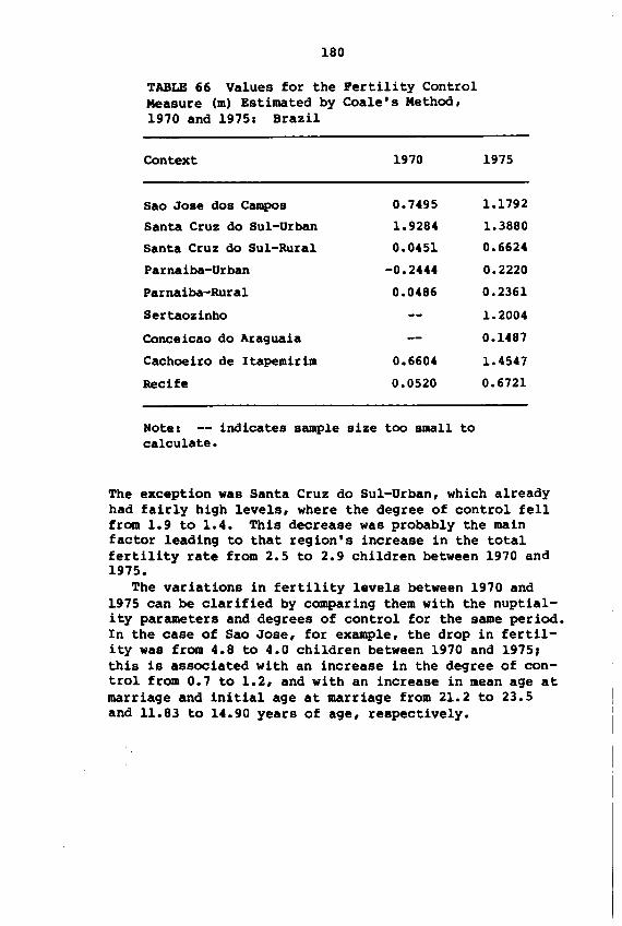
180

TABLE 66 Values for the Fertility ControlMeasure (m) Estimated by Coale's Method,1970 and 1975: Brazil

Context

Sao Jose dos Campos

Santa Cruz do Sul-Urban

Santa Cruz do Sul-Rural

Parnaiba-Urban

Parnaiba-Rural

Sertaozinho

Conceicao do Araguaia

Cachoeiro de Itapemirim

Recife

1970

0.7495

1.9284

0.0451

-0.2444

0.0486

0.6604

0.0520

1975

1.1792

1.3880

0.6624

0.2220

0.2361

1.2004

0.1487

1.4547

0.6721

Note: -- indicates sample size too small tocalculate.

The exception was Santa Cruz do Sul-Urban, which alreadyhad fairly high levels, where the degree of control fellfrom 1.9 to 1.4. This decrease was probably the mainfactor leading to that region's increase in the totalfertility rate from 2.5 to 2.9 children between 1970 and1975.

The variations in fertility levels between 1970 and1975 can be clarified by comparing them with the nuptial­ity parameters and degrees of control for the same period.In the case of Sao Jose, for example, the drop in fertil­ity was from 4.8 to 4.0 children between 1970 and 1975,this is associated with an increase in the degree of con­trol from 0.7 to 1.2, and with an increase in mean age atmarriage and initial age at marriage from 21.2 to 23.5and 11.83 to 14.90 years of age, respectively.

CHAPTER 9

THE PROXIMATE VARIABLES

The factors that directly influence fertility and togetherdetermine its level--the so-called proximate variables-­can be grouPed as follows, according to Bongaarts (1983),

a) exposure to regular sexual relationsproportion of married women

b) prevalence of deliberate control of maritalfertility

use and efficiency of contraceptivesprevalence of induced abortion

c) determinants of natural marital fertilityduration of postpartum infecundityfecundityspontaneous intrauterine mortalityprevalence of permanent sterility

However, not all these factors have the same impact indetermining discrepancies between natural fertility andthe total fertility rates observed in a given context.In fact, the proportion of married women, the use andefficiency of contraceptives, the prevalence of inducedabortion, and the duration of postpartum infecundityaccount in general for over 95 percent of those discrep­ancies, the effects of the remaining three factors aredifficult to measure in such studies as fertility surveys.Postpartum infecundity depends in turn on the length ofsexual abstention following delivery and on the durationof breastfeeding. In Latin America, prolonged abstinenceis not as common a practice as it is in some African andAsian countries. As can be seen in Table 67, in the HIHR,a limited number of women declared they abstained. On theother hand, what does still exist among some groups ofwomen of rural origin is -postpartum quarantine- or -re-

181

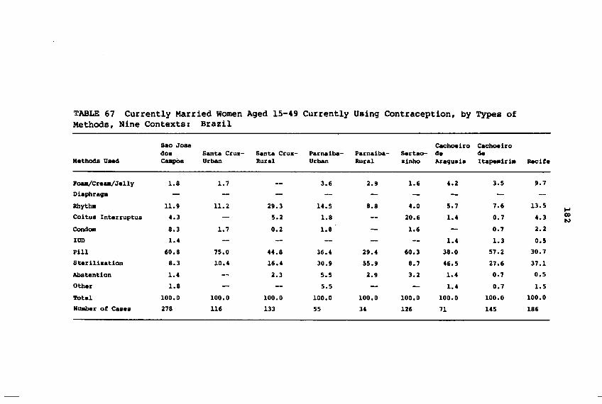
TABLE 67 Currently Married Women Aged 15-49 Currently Using Contraception, by Types ofMethods, Nine Contexts: Brazil

Sao Jose Cacboeiro Cacboeirodos Santa Cru:l- Santa Cru:l- Parnaiba- Parnaiba- Serteo- de de

Metllods OHd CaapOs Urban Rural Urban Rural :linbo Araguaia Ite~iria Recife

POlUI/Cre811/Jelly 1.8 1.7 -- 3.6 2.9 1.6 4.2 3.5 9.7

Diaphra91ll

Rhytlul 11.9 11.2 29.3 14.5 8.8 4.0 5.7 7.6 13.5~

Coitus Interruptus 4.3 - 5.2 1.8 - 20.6 1.4 0.7 4.3 CDN

Condoe 8.3 1.7 0.2 1.8 - 1.6 - 0.7 2.2

IUD 1.4 -- -- - - -- 1.4 1.3 0.5

pill 60.8 75.0 44.8 36.4 29.4 60.3 38.0 57.2 30.7

Sterilization 8.3 10.4 16.4 30.9 55.9 8.7 46.5 27.6 37.1

Abstention 1.4 -- 2.3 5.5 2.9 3.2 1.4 0.7 0.5

Other 1.8 -- -- 5.5 - - 1.4 0.7 1.5

Total 100.0 100.0 100.0 100.0 100.0 100.0 100.0 100.0 100.0

HllIIber of Cases 278 116 133 55 34 126 71 145 186

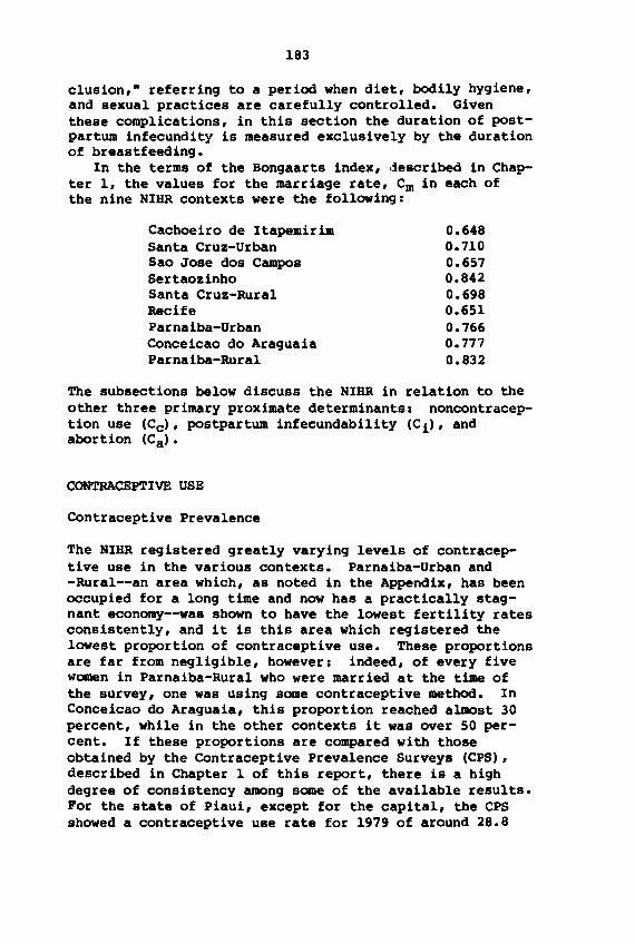
183

clusion,· referring to a period when diet, bodily hygiene,and sexual practices are carefully controlled. Giventhese complications, in this section the duration of post­partum infecundity is measured exclusively by the durationof breastfeeding.

In the terms of the Bongaarts index, described in Chap­ter 1, the values for the marriage rate, Cm in each ofthe nine NIHR contexts were the following:

Cachoeiro de ItapemirimSanta Cruz-UrbanSao Jose dos CamposSertaozinhoSanta Cruz-RuralRecifeParnaiba-UrbanConceicao do AraguaiaParnaiba-Rural

0.6480.7100.6570.8420.6980.6510.7660.7770.832

The subsections below discuss the NIHR in relation to theother three primary proximate determinants: nonoontracep­tion use (Cc)' postpartum infecundability (Ci)' andabortion (Ca).

CONTRACEPTIVE USE

Contraceptive Prevalence

The NIHR registered greatly varying levels of contracep­tive use in the various contexts. Parnaiba-Urban and-Rural--an area which, as noted in the Appendix, has beenoccupied for a long time and now has a practically stag­nant economy--was shown to have the lowest fertility ratesconsistently, and it is this area which registered thelowest proportion of contraceptive use. These proportionsare far from negligible, however: indeed, of every fivewomen in Parnaiba-Rural who were married at the time ofthe survey, one was using some contraceptive method. InConceicao do Araguaia, this proportion reached almost 30percent, while in the other contexts it was over 50 per­cent. If these proportions are compared with thoseobtained by the Contraceptive Prevalence Surveys (CPS),described in Chapter 1 of this report, there is a highdegree of consistency among some of the available results.For the state of Piaui, except for the capital, the CPSshowed a contraceptive use rate for 1979 of around 28.8

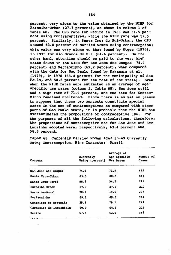
184

percent, very close to the value obtained by the NIHR forParnaiba-Urban (27.7 percent), as shown in column 1 ofTable 68. The CPS rate for Recife in 1980 was 51.5 per­cent using contraceptives, while the NIHR rate was 57.5percent. Similarly, in Santa Cruz do Sul-Urban, the CPSshowed 63.0 percent of married women using contraception;this value was very close to that found by Etges (1976),in 1975 for Rio Grande do Sul (64.6 percent). On theother hand, attention should be paid to the very highrates found in the NIHR for Sao Jose dos Campos (74.9percent) and Sertaozinho (69.2 percent), when comparedwith the data for Sao Paulo found by Nakamura et al.(1979), in 1978 (63.4 percent for the municipality of SaoPaulo, and 58.6 percent for the rest of the state). Evenwhen the NIHR rates were estimated as an average of age­specific use rates (column 2, Table 68), Sao Jose stillhad a high rate of 71.9 percent, and the rate for Sertao­zinho remained unaltered. Since there is as yet no reasonto suppose that these two contexts constitute specialcases in the use of contraceptives as compared with otherparts of Sao Paulo state, it is probable that the NIHR hasoverestimated the proportions of contraceptive use. Forthe purposes of all the following calculations, therefore,the proportions of contraceptive use for Sao Jose and Ser­taozinho adopted were, respectively, 63.4 percent and58.6 percent.

TABLE 68 Currently Married Women Aged 15-49 CurrentlyUsing Contraception, Nine Contexts: Brazil

Average ofCurrently Age-Specific Number of

Context Using (percent) Use Rates CAses

Sao Jose dos Campos 74.9 71.9 475

Santa Cruz-Urban 63.0 60.6 219

Santa Cruz-Rural 58.3 54.3 242

Parnaiba-Urban 27.7 27.7 220

Parnaiba-Rural 20.7 19.6 207

Sertaozinho 69.2 69.3 224

Conceicao do Araguaia 29.6 29.1 274

Cachoeiro do Itapeairia 69.9 64.5 229

Recife 57.5 52.0 348

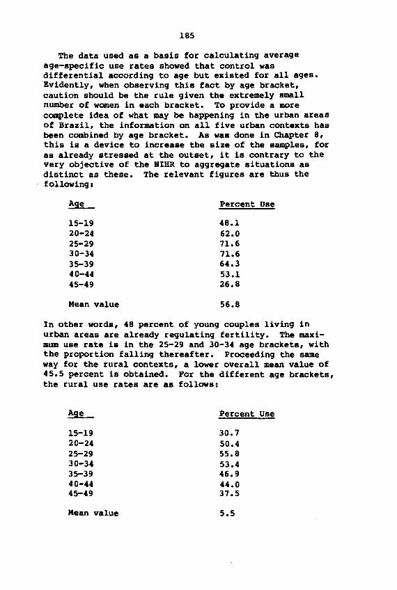
185

The data used as a basis for calculating averageage-specific use rates showed that control wasdifferential according to age but existed for all ages.Evidently, when observing this fact by age bracket,caution should be the rule given the extremely smallnumber of women in each bracket. To provide a morecomplete idea of what may be happening in the urban areasof Brazil, the information on all five urban contexts hasbeen combined by age bracket. As was done in Chapter 8,this is a device to increase the size of the samples, foras already stressed at the outset, it is contrary to thevery objective of the HIHR to aggregate situations asdistinct as these. The relevant figures are thus thefollowing:

~ Percent Use

15-19 48.120-24 62.025-29 71.630-34 71.635-39 64.340-44 53.145-49 26.8

Mean value 56.8

In other words, 48 percent of young couples living inurban areas are already regulating fertility. The maxi­mum use rate is in the 25-29 and 30-34 age brackets, withthe proportion falling thereafter. Proceeding the sameway for the rural contexts, a lower overall mean value of45.5 percent is obtained. For the different age brackets,the rural use rates are as follows:

~ Percent Use

15-19 30.720-24 50.425-29 55.830-34 53.435-39 46.940-44 44.045-49 37.5

Mean value 5.5

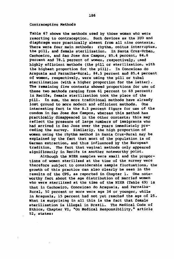
186

Contraceptive Methods

Table 67 shows the methods used by those women who wereresorting to contraception. Such devices as the IUD anddiaphragm were practically absent from all nine contexts.There were four main methodsl rhythm, coitus interruptus,the pill, and female sterilization. In Santa Cruz-Urban,Cachoeiro, and Sao Jose dos Campos, 85.4 percent, 84.8percent and 78.1 percent of women, respectively, usedhighly efficient methods (the pill or sterilization, withthe highest proportion for the pill). In Conceicao doAraguaia and Parnaiba-Rural, 84.5 percent and 85.4 percentof women, respectively, were using the pill or tubalsterilization (with a higher proportion for the latter) •The reaaining five contexts showed proportions for use ofthese two methods ranging from 61 percent to 69 percentJin Recife, female sterilization took the place of thepill. In sum, the more traditional methods have alreadylost ground to more modern and efficient methods. Oneinteresting fact is the 8.3 percent figure for use of thecondom in Sao Jose dos Campos, whereas this method haspractically disappeared in the other contextsJ this mayreflect the presence of large numbers of immigrants whohad arrived in Sao Jose over the years immediately pre­ceding the survey. Similarly, the high proportion ofwomen using the rhythm method in Santa Cruz-Rural may beexplained by the fact that most of the population is ofGerman extraction, and thus influenced by the Europeantradition. The fact that vaginal methods only appearedsignificantly in Recife is another noteworthy point.

Although the NIHR samples were small and the propor­tions"of women sterilized at the time of the survey weretherefore subject to considerable sample fluctuations, thegrowth of this practice can also clearly be seen in theresults of the CPS, as reported in Chapter 1. One note­worthy fact about the age distribution of married womenwho were sterilized at the time of the NIHR (Table 69) isthat in Cachoeiro, Conceicao do Araguaia, and Parnaiba­Rural, 50 percent or more were age 34 or younger, whilein Araguaia, 15 percent had not yet reached the age of 25.What is surprising in all this is the fact that femalesterilization is illegal in Brazil. The Medical Code ofEthics, Chapter VI, ·On Medical Responsibility,· article52, states:

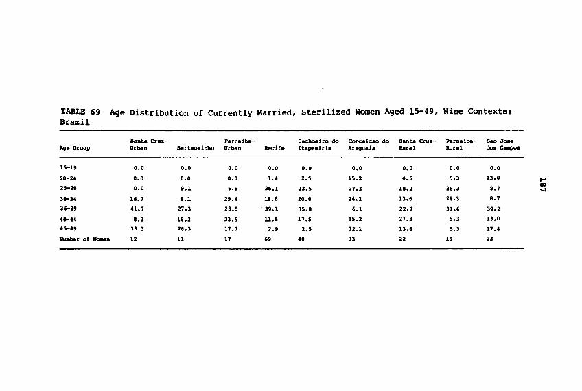
TABLE 69 Age Distribution of Currently Married, sterilized Women Aged 15-49, Nine Contexts:Brazil

Santa Cru,,- Parnalba- Cachoelro do Coneelcao do Santa Cru,,- Parnaiba- SIlO JoeeAge Group Urban Sartaodnho Urban Recife Itapeald. Ara9uala Rural Rural doe CuIpoe

15-19 0.0 0.0 0.0 0.0 0.0 0.0 0.0 0.0 0.0

20-24 0.0 0.0 0.0 1.4 2.5 15.2 4.5 5.3 13.0 ....25-29 0.0 9.1 5.9 26.1 22.5 27.3 18.2 26.3 8.7

CD-..I

30-34 16.7 9.1 29.4 18.8 20.0 24.2 13.6 26.3 8.7

35-39 41.7 27.3 23.5 39.1 35.0 6.1 22.7 31.6 39.2

40-44 8.3 18.2 23.5 11.6 17.5 15.2 27.3 5.3 13.0

45-U 33.3 26.3 17.7 2.9 2.5 12.1 13.6 5.3 17.4

llullber of we-en 12 11 17 69 40 33 22 19 23

188

Sterilization is condemned, but may be practised inexceptional cases, when there is a precise indica­tion approved by two medical doctors consulted inconference.

Aside from the few cases in which a woman's health prob­lems lead to the advisability of sterilization, the markedincrease in tubal sterilization among Brazil's femalepopulation may be the result of two factors.

The first is a consequence of the misuse of caesareansover recent years, this has been stimulated by the INAMPS(National Health and Welfare Service) through higherremuneration for this kind of operation than for normaldelivery. Official data show that from 1971 to 1980 inBrazil, the proportion of caesareans to total deliveriesrose from 14.6 percent to 29.3 percent. The rates for SaoPaulo over the same period rose from 17.5 percent to 36.0percent, and similar increases occurred in practically allthe Brazilian states.ll A study performed in RibeiraoPreto, Sao Paulo state, concerning standards of assistancefor deliveries showed that in 1972, 1973, and 1974, 18.1percent, 23.0 percent, and 24.1 percent of hospitaldeliveries, respectively, were caesareans (Boletin de laOficina Sanitaria Panamerican, 1978). Recent data onGreater Sao Paulo and Greater Recife permit a comparisonbetween the type of delivery of the latest and penultimatechildren born to mothers who gave birth over the last 8months (Berquo, 1981). The results for Greater Recifeshow that 14 percent of deliveries of the penultimatechild were caesareans, while the rate is 27 percent forthe latest child. In addition, 11 percent of thesemothers gave birth by caesarean in both cases. Forgreater Sao Paulo, 21 percent of deliveries were caesar­eans for the penultimate child and 31 percent for thelatest, while 17 percent of these mothers had given birthby caesarean in both cases. It is well known that anywoman who has already had two or three caesareans is asure candidate for sterilization. The policy adopted byINAMPS has thus increased women's chances of being ster­ilized. Nowadays, in fact, doctors receive the sameremuneration whether a delivery is normal or caesarean;nevertheless, it seems that the doctors themselves havegrown accustomed to caesarean deliveries and thus continuepersuading pregnant women to accept them, with a continu­ing effect on sterilization levels.

The second factor which may determine the markedincrease in tubal sterilization is linked to the non-

189

official family planning programs underway in Brazil. Asnoted in Chapter 3, physicians in private practive havebeen making more frequent use of public facilities to per­form sterilizations even though use is not officiallypromoted. If this were not so, given the legislationmentioned earlier, these results would not be occurringand affecting even very young women, as seen in the datashown here.

Bongaarts' Index of Contraception

In calculating the Bongaarts contraception index (Cc •1 - S x E x U), described in Chapter 1, the values for·U· are already available in the second column of Table68. Values for ·E· in any given context are calculatedby adding the products of the values in Table 63 and theweights which correspond to each of the methods inaccordance with its efficiency:

Methods

Foam/Cream JellyDiaphragmRhythmCondom100PillSterilizationAbstentionOther

Contraceptive Efficiency

0.870.880.820.910.960.981.001.000.90

Values for ·E· thus calculated are shown in Table 70. If·U·, ·E·, and ·S· are replaced in the formula for Cc bytheir respective values, the results obtained are as shownin Table 71.

As can be seen, the degree of control is greatest inCachoeiro de Itapemirim, followed by Sao Jose and SantaCruz do Sul-Urban. The lowest values of Cc are forConceicao do Araguaia and Parnaiba-Urban and -Rural. Inother words, these results confirm the findings obtainedwhen ·m· was calculated by Coale's method. The relationbetween the values for Cc and total fertility is alsovery clear: that is, the lower the value for Cc, thelower the total fertility rate.

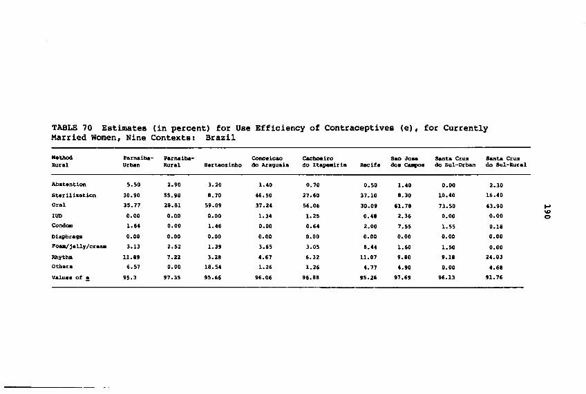
TABLE 70 Estimates (in percent) for Use Efficiency of Contraceptives (e) , for CurrentlyMarried Women, Nine Contexts: Brazil

Method Parneiba- Parnaiba- Conceicao eacboeiro sao JOM Santa Cruz Santa CruzRural Urban Rural Sertaodnho do Araguaia do Itapeairi. Recife dos caapos do Sul-Urban do Sul-Rural

Abstention 5.50 2.90 3.20 1.40 0.70 0.50 1.40 0.00 2.30

Sterilbation 30.90 55.90 S.70 46.50 27.60 37.10 S.30 10.40 16.40

Oral 35.77 2S.S1 59.09 37.24 56.06 30.09 61.7S 73.50 43.90 ~ID

IUD 0.00 0.00 0.00 1.34 1.25 o.n 2.36 0.00 0.00 0

CondOll 1.64 0.00 1.46 0.00 0.64 2.00 7.55 1.55 0.18

Diaphragll 0.00 0.00 0.00 0.00 0.00 0.00 0.00 0.00 0.00

Poaa/jel1y/cre.. 3.ll 2.52 1.39 3.65 3.05 8.U 1.60 1.50 0.00

Rhythll 11.89 7.22 3.28 4.67 6.32 11.07 9.80 9.18 24.03

Others 6.57 0.00 18.54 1.26 1.26 4.77 4.90 0.00 4.68

Values ot ~ 95.3 97.35 95.66 96.06 96.88 95.26 97.69 96.13 91.76

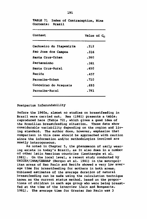
TABLE 71Contexts:

Context

191

Index of Contraception, NineBrazil

Value of Co

Cachoeiro do Itapemirim .312

Sao Jose dos Campos .316

Santa Cruz-Urban .360

Sertaozinho .381

Santa Cruz-Rural .450

Recife .457

Parnaiba-Urban .710

Conceicao do Araguaia .693

Parnaiba-Rural .791

Postpartum Infecundability

Before the 1960s, almost no studies on breastfeeding inBrazil were carried out. Rea (1981) presents a table,reproduced here (Table 72), which gives a good idea ofthe Brazilian breastfeeding situation. These data showconsiderable variability depending on the region and liv­ing standard. The author does, however, emphasize thatcomparison in this case should be approached with cautionsince the information and/or methodologies involved aremostly heterogeneous.

As noted in Chapter 5, the phenomenon of early wean­ing exists in today's Brazil, as it also does in a numberof other Latin American countries (Lesthaeghe et al.1981). On the local level, a recent study conducted byUNICEF/INAM/CEBRAP (Berquo et al. 1981) in the metropol­itan areas of Sao Paulo and Recife showed a very low aver­age time for breastfeeding for mothers in both areas.Unbiased estimates of the average duration of naturalbreastfeeding can be made using the calculation techniqueknown as the current status method, based on the propor­tions of children in each age group who were being breast­fed at the time of the interview (Jain and Bongaarts,1981). The average time for Greater Sao Paulo was 3

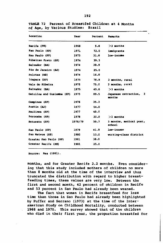
192

TABLE 72 Percent of Breastfed Children at 4 Monthsof Age, by Various Studies: Brazil

Salvador (DA) 1975

Getulina and Guaiellbe (SP) 1975

Location

Recife (PI:)

Sao Paulo (SP)

Sao Paulo (SP)

Ribeirao Preto (SP)

Salvador (DA)

Rio de Janeiro (RJ)

Pe10ta. (RS)

leapara (SP)

Vale do Ribeira

CUlpina. (SP)

AusUn (RJ)

Paulinea (SP)

Sorocaba (SP)

Botucatu (SP)

Sao Paulo (SP)

Sao Mateu. (SP)

Greater Sao Paulo (SP)

Greater Recife (PI:)

Source: Rea (1981).

Ye.r

1968

1971

1973

1974

1974

1974

1974

1975

1975

1976

1977

1977

1978

1978/79

1979

1980

1981

1981

Percent

5.8

72.0

31.6

39.3

38.9

25.0

16.0

78.8

75.0

45.0

89.5

35.3

54.0

40.0

30.0

50.7

41.9

13.0

38.0

25.0

Rellark.

>3.anth.

i..igrantB

low-incaae

3 .anth., rural

3 IROnth., rural

>3.anth.

Japane.e extraction, 3IROnth.

>3 IROnth.

3 IROnth., medical po.t,school

low-incOllle

workingooc1as. district

months, and for Greater Recife 2.2 months. Even consider­ing that this study included mothers of children no morethan 8 months old at the time of the interview and thustruncated the distribution with regard to higher breast­feeding times, these values are very low. Between thefirst and second month, 42 percent of children in Recifeand 53 percent in Sao Paulo had already been weaned.

The fact that women in Recife breastfeed for lesstime than those in Sao Paulo had already been highlightedby Puffer and Serrano (1973) at the time of the Inter­american Study on Childhood Mortality, conducted between1968 and 1970. This survey showed that of the childrenwho died in their first year, the proportion breastfed for

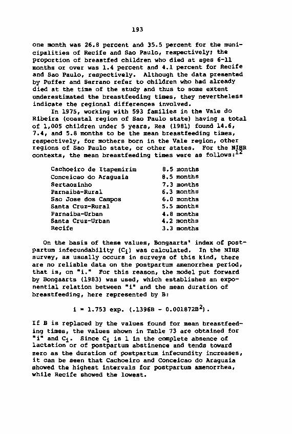
193

one month was 26.8 percent and 35.5 percent for the muni­cipalities of Recife and Sao Paulo, respectively, theproportion of breastfed children who died at ages 6-11months or over was 1.4 percent and 4.1 percent for Recifeand Sao Paulo, respectively. Although the data presentedby Puffer and Serrano refer to children who had alreadydied at the time of the study and thus to some extentunderestimated the breastfeeding times, they neverthelessindicate the regional differences involved.

In 1975, working with 593 families in the Vale doRibeira (coastal region of Sao Paulo state) having a totalof 1,005 children under 5 years, Rea (1981) found 14.6,7.4, and 5.8 months to be the mean breastfeeding times,respectively, for mothers born in the Vale region, otherregions of Sao Paulo state, or other states. For the NI~

contexts, the mean breastfeeding times were as follows: l

Cachoeiro de ItapemirimConceicao do AraguaiaSertaozinhoParnaiba-RuralSao Jose dos CamposSanta Cruz-RuralParnaiba-UrbanSanta Cruz-UrbanRecife

8.5 months8.5 months7.3 months6.3 months6.0 months5.5 months4.8 months4.2 months3.3 months

On the basis of these values, Bongaarts' index of post­partum infecundability (Ci) was calculated. In the NIHRsurvey, as usually occurs in surveys of this kind, thereare no reliable data on the postpartum amenorrhea period,that is, on -i.- For this reason, the model put forwardby Bongaarts (1983) was used, which establishes an expo­nential relation between -i- and the mean duration ofbreastfeeding, here represented by B:

i = 1.753 expo (.1396B - 0.001872B2).

If B is replaced by the values found for mean breastfeed­ing times, the values shown in Table 73 are obtained for-i- and Ci. Since Ci is 1 in the complete absence oflactation or of postpartum abstinence and tends towardzero as the duration of postpartum infecundity increases,it can be seen that Cachoeiro and Conceicao do Araguaiashowed the highest intervals for postpartum amenorrhea,while Recife showed the lowest.

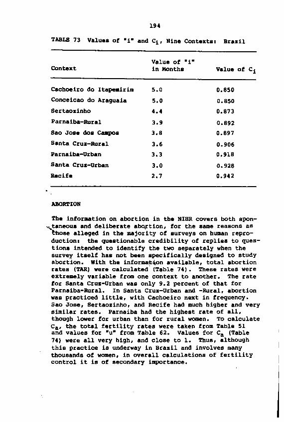
194

TABLE 73 Values of ·i· and Ci, Nine Contextsl Brazil

Value of ·i·Context in Months Value of Ci

Cachoeiro do Itapeairim 5.0 0.850

Conceicao do Araguaia 5.0 0.850

Sertaozinho 4.4 0.873

Parnaiba-Rural 3.9 0.892

Sao Jose dos C.-pos 3.8 0.897

Santa Cruz-Rural 3.6 0.906

Parnaiba-Orban 3.3 0.918

Santa Cruz-Orban 3.0 0.928

Recife 2.7 0.942

ABORTION

The inforaation on abortion in the NIHR covers both spon-~taneous and deliberate a~tion, for the same reasons as

those alleged in the majority of surveys on human repro­ductionl the questionable credibility of replies to ques­tions intended to identify the two separately when thesurvey itself has not been specifically designed to studyabortion. With the informa~n available, total abortionrates (TAR) were calculated (Toble 74). These rates wereextremely variable from one context to another. The ratefor Santa Cruz-Orban was only 9.2 percent of that forParnaiba-Rural. In Santa Cruz-Orban and -Rural, abortionwas practiced little, with Cachoeiro next in frequency.Sao Jose, Sertaozinho, and Recife had much higher and verysimilar rates. Parnaiba had the highest rate of all,though lower for urban than for rural women. To calculateCa , the total fertility rates were taken from Table 51and values for ·u· from Table 62. Values for Ca (Table74) were all very high, and close to 1. Thus, althoughthis practice is underway in Brazil and involves manythousands of women, in overall calculations of fertilitycontrol it is of secondary importance.

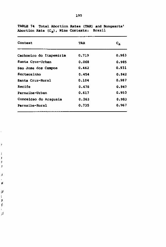
I~

lIeq\

195

TABLE 74 Total Abortion Rates (TAR) and Bongaarts 'Abortion Rate (Ca), Nine Contexts: Brazil

Context TAR Ca

Cachoeiro do Itapemirim 0.719 0.963

Santa Cruz-Urban 0.068 0.985

Sao Jose dos Campos 0.462 0.931

Sertaozinho 0.454 0.942

Santa Cruz-Rural 0.104 0.987

Recife 0.478 0.947

Parnaiba-Urban 0.617 0.953

Conceicao do Araguaia 0.263 0.983

Parnaiba-Rural 0.735 0.967

CHAPTER 10

SOCIOECON<»(IC FACTORSI FAMILY INCOME

As pointed out in Chapter S, the fertility rates observedfor each of the nine NIHR contexts varied considerably.Succeeding chapters showed that, at least at this levelof analysis, a variety of reproduction strategies havebeen adopted by the populations of the different contexts.The present chapter incorporates into the analysis thesocioeconomic variables. Among these, family incomeappears to have distinctive importance and is the focusof the discussion that follows.

The analysis below is limited to the urban contextssince it addresses only monetary income. Families havebeen classified in four categories, depending on their percapita monthly income at the time of the survey (between1975 and 1977):

(1) up to one-half the minimum wage 13(2) between one-half and one minimum wage(3) between one and two times the minimum wage(4) over twice the minimum wage

This variable has been incorporated into the analysisaccording to its equivalent at the particular moment ofthe time of interviewJ this precaution was taken since theinformation concerned was not taken from the individuallife histories, but from data included in the form dealingwith the domestic group. Although this disparity makesinterpretation of the results somewhat problematic, thepresent analysis is only preliminarYJ later research willbe able to incorporate variables from the life histories.

The distribution of families according to income (Table75) varies considerably from one context to the next. Onthe one hand, Santa Cruz, Cachoeiro, and Sao Jose dosCampos are somewhat similar, showing a degree of equili-

196

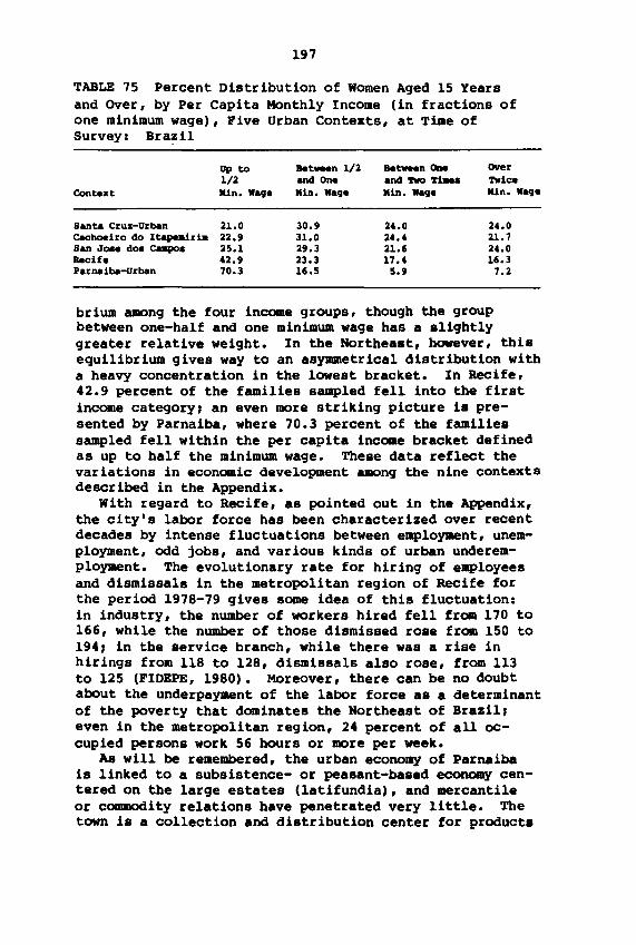
197

TABLE 75 Percent Distribution of Women Aged 15 Yearsand Over, by Per Capita Monthly Income (in fractions ofone minimum wage), Five Urban Contexts, at Tiae ofSurvey: Brazil

Up to Bet_n 1/2 Be~n One OVer1/2 and One and 'rIlo 'l'~a '1'Wic.

Context Ilin. Wag. Ilin. Wag. Ilin. Wag. Ilin. Wag.

Santa Crus-Urban 21.0 30.9 24.0 24.0Cachoeiro do ltape.iri. 22.9 31.0 24.4 21.7San Joae doa CaiIpoa 25.1 29.3 21.6 24.0Recife 42.9 23.3 17.4 16.3Parnaiba-Urban 70.3 16.5 5.9 7.2

brium among the four income groups, though the groupbetween one-half and one minimum wage has a slightlygreater relative weight. In the Northeast, however, thisequilibrium gives way to an asymmetrical distribution witha heavy concentration in the lowest bracket. In Recife,42.9 percent of the families sampled fell into the firstincome category, an even more striking picture is pre­sented by Parnaiba, where 70.3 percent of the familiessampled fell within the per capita income bracket definedas up to half the minimum wage. These data reflect thevariations in economic development among the nine contextsdescribed in the Appendix.

With regard to Recife, as pointed out in the Appendix,the city's labor force has been characterized over recentdecades by intense fluctuations between employment, unem­ployment, odd jobs, and various kinds of urban underem­ployment. The evolutionary rate for hiring of e~loyees

and dismissals in the metropolitan region of Recife forthe period 1978-79 gives some idea of this fluctuation:in industry, the number of workers hired fell from 170 to166, while the number of those dismissed rose from 150 to194, in the service branch, while there was a rise inhirings from 118 to 128, dismissals also rose, from 113to 125 (FIDEPE, 1980). Moreover, there can be no doubtabout the underpayment of the labor force as a determinantof the poverty that dominates the Northeast of Brazil,even in the metropolitan region, 24 percent of all oc­cupied persons work 56 hours or more per week.

As will be remembered, the urban economy of Parnaibais linked to a subsistence- or peasant-based economy cen­tered on the large estates (latifundia), and mercantileor commodity relations have penetrated very little. Thetown is a collection and distribution center for products

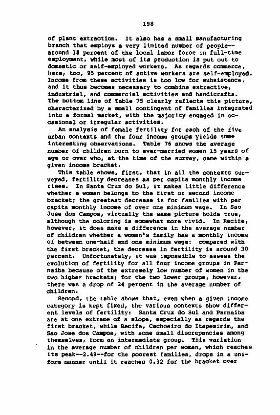
198

of plant extraction. It also has a small manufacturingbranch that employs a very limited number of people-­around 18 percent of the local labor force in full-timeemployment, while most of its production iB put out todomestic or self-employed workers. As regards commerce,here, too, 95 percent of active workerB are Belf-employed.Income from these activities is too low for SubBiBtence,and it thus becomeB necesBary to combine extractive,industrial, and commercial activities and handicrafts.The bottom line of Table 75 clearly reflectB thiB picture,characterized by a Bmall contingent of families integratedinto a formal market, with the majority engaged in oc­casional or irregular activities.

An analysis of female fertility for each of the fiveurban contexts and the four income groups yields someinteresting observations. Table 76 shows the averagenumber of children born to ever-married women 15 years ofage or over who, at the time of the survey, came within agiven income bracket.

This table shows, firBt, that in all the contexts sur­veyed, fertility decreaBes as per capita monthly incomeriBes. In Santa Cruz do Sul, it makeB little differencewhether a woman belongs to the first or second incomebracket, the greatest decrease iB for families with percapita monthly income of over one minimum wage. In SaoJose dos Campos, virtually the same picture holdB true,although the coloring is Bomewhat more vivid. In Recife,however, it does make a difference in the average numberof children whether a woman's family has a monthly incomeof between one-half and one minimum wage: compared withthe first bracket, the decreaBe in fertility iB around 30percent. Unfortunately, it was impossible to aBsess theevolution of fertility for all four income groups in Par­naiba because of the extremely low number of women in thetwo higher brackets, for the two lower groups, however,there was a drop of 24 percent in the average number ofchildren.

Second, the table Bhows that, even when a given incomecategory is kept fixed, the various contextB Bhow differ­ent levels of fertility: Santa Cruz do Sul and Parnaibaare at one extreme of a slope, especially as regards thefirst bracket, while Recife, Cachoeiro do Itapemirim, andSao Jose dos Ca.pos, with some small discrepancies amongthemselves, form an intermediate group. ThiB variationin the average number of children per woman, which reachesits peak--2.49--for the POOreBt families, dropB in a uni­form manner until it reaches 0.32 for the bracket over

TABLE 76 Average Number of Children Born to Ever-Married Women Aged lS and Over, byPer Capita Monthly Income (in fractions of one minimum wage), Pive Urban Contexts: Brazil

(2) (3) (6) Percentage Decrease(1) Between Between 1 OverUp to 1/2 1/2 and and 2 Ti_s Twice

Urban Contexts Min. Wage 1 M. W. Min. Wage M. W. (2)/11) (3)/12) (6) /(3) (6)/11)

Santa Cruz do Su1 3.37 2.96 2.29 1.76 12 23 27 50 ....IDID

Recife 6.28 3.05 3.33 1.87 30 10 U 56

Cachoeiro 6.39 3.38 2.61 2.06 21 27 16 53

Sao Jose dos Ca.pos 6.97 6.23 2.96 1.96 16 32 35 62

Parnaiba 5.86 6.69 -- -- 26

Maxia~ Difference 2.69 1.53 1.06 0.32

200

twice the mini.ua wage. If Parnaiba is eliminated fromthe comparison (since the reduction in the variation maybe influenced by the fact that Parnaiba is not representedin the two higher income brackets), the maximum differencebetween the contexts for the four brackets would then be,respectively, 1.60, 1.27, 1.04, and 0.32. In other words,the decrease in the variation between contexts as the percapita monthly income of the families rises is a persis­tent trend.

This trend may well reflect, among other things, theeffect of the population's degree of involvement in theformal labor market. Such involvement requires moreskill, reflected, for example, in a higher level ofschooling, it also exposes people to a mass of informationrelated to health, hygiene, sex, and reproduction. InSao Jose dos Campos, for example, a survey of the bigcompanies, mainly the mUltinationals, showed that socialworkers within the companies present the idea of planningto employees whose productivity is falling off, this plan­ning includes the reduction of fertility. In their studyof social institutions and reproductive behavior, Loyolaand Quinteiro (1982:43) make the following point:

• • • social institutions were observed to actbasically along ·controlist· lines, i.e., theyinduce or transmit, in an explicit or diffuse man­ner, the pattern of the small conjugal family, whosecorollary is the idea of birth control. Accordingto the viewpoint of the institutional agents, sucha reproductive pattern is associated -- again at allpoints of the survey in general -- to economic andsocial problems (poverty, cost of living, socialmarginality, etc.) and appears as a solution offeredto such problems in the short or long term.

However, as Loyola and Quintero note further (pp.43-45), this institutional role varies significantly fromone institution and from one context to another.

Thus, to give one example of a contextual variation,the most general references to social problems can,in a large town in the South undergoing intenseindustrialization and with full employment (the caseof Sao Jose dos Campos at the time of the survey) ,be translated into other, more specific referenceswhich basically concern the disorganizing effectson the social fabric of the excessively intense pace

201

of industrialization and immigrationJ in Parnaibaor Recife, they may take on the connotation of back­wardness as compared with the South, while situa­tions of unemployment and underemployment may beseen as non-residual realities which affect thepopulation as a whole through their pathologicalconsequences I abandoned minors, prostitution(Parnaiba and Recife), marginality and criainality(Recife).

Finally, it should be noted that, in addition to thebasic criteria used to select the NIHR urban contexts--theprevailing form of organization of production and thesocial division of labor--or perhaps even as a result ofthese criteria, the contexts have specific features thatmay help to explain fertility levels. Thus in 1950, SantaCruz do Sul, a region with a large population of Germanorigin, already had a fertility rate considered low byBrazilian standardsJ moreover, family size in Santa Cruzhas been highly influenced by property size, which hasfallen gradually over the last few decades because of thesuccessive sharing of inheritances among survivingchildren.

CBAPTBR 11

COHCWSIONS

DECC»IPOSITION OJ!' GENERAL FERTILITY RATES

The contribution of change. in age structure, maritalstatus, and marital fertility to declines in general fer­tility rates in 1970-75 is shown for the nine contexts inTable 77. The standardization procedure used (see UnitedNations, 1979), taking 1970 as the base year, shows thatthe three factors play specific roles in reducing fertil­ity in the different contexts and that distinct interac­tion effects are also present.

As can be seen, over the period considered, the declinein the general fertility rate varied a great deal from onecontext to another, as has already been observed withregard to total fertility rates. The largest fall, inSertaozinho, was around 67.43 per 1,000 (174.70-107.27).At the other extreme was Santa Cruz-Urban (90.41-83.75),with 6.65 per 1,000. Cachoeiro de Itapemirim, Sao Josedos Campos (154.49-140.20), Recife (174.85-162.00), andConceicao do Araguaia (236.26-225.70) showed similardeclines, which varied from 11 to 15 per 1,000, Parnaiba­Urban (227.94-185.12) and Santa Cruz-Rural (190.48-149.28)had larger declines of around 40 per 1,000. The onlyexception was Parnaiba-Rural (250.49-273.26), with agrowth of 22.27 per 1,000 between 1970 and 1975.

In all the contexts where there was a reduction in thegeneral fertility rate, except for Santa Cruz-Urban, thedecline in marital fertility was the most directlyresponsible factor. In Cachoeiro, Recife, Sao Jose, andAraguaia, the decline can be totally explained by thereduction in marital fertility, and would have been evenlarger if age structure and marital status had not con­tributed to the attenuation of this reduction. In Cacho­eiro, Recife, and Araguaia, the contribution of marital

202

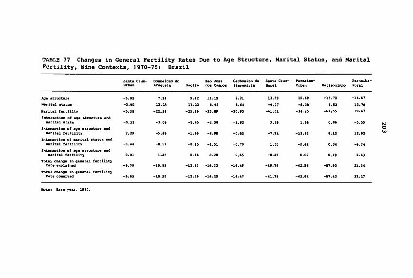
TABLE 77 Changes in General Fertility Rates Due to Age Structure, Marital Status, and MaritalFertility, Nine Contexts, 1970-75: Brazil

Banta Crul- Cone.LeBO do Sao Jo.. caeboelro de Santa Cruz- Parnalba- Parnalba-Orban Araguaia Raclf. doe CUIpoe Itapaairia "'ral Orban IIertaoo1nho "'ral

-12.86 -14.2'

Age structure

Marital atatus

IIarital fertility

Interactton of &ge structure and••rital atat.

Interaction of &ge structure andaerital f.rtility

Interaction of ..rital atatue andaerital f.rtility

Interaction of age structure andaerital f.rtility

Total chang. in g.neral f.rtilityrate explained

Total chang. in g....ral fertilityrate obeerved

IIote I sa•• ye.r, 1970.

-5.05

-2.'0

-5.36

-0.33

7.2'

-0.44

0.01

-6.79

-6.65

7.24

13.25

-22.34

-3.06

-5.&&

-0.57

1.46

-10.'8

-10.56

'.12

11.23

-25.'5

-5.45

-1."-0.15

0.46

-12.43

11.15

8.42

-25.0'

-2.58

-4.88

-1.51

0.20

-14.33

2.21

6.64

-20.85

-1.82

-0.&2

-0.70

0.65

-14.4'

-14.47

13.5'

-'.77-41.51

3.71

-7.92

1.50

-0.46

-40.79

-41.79

10."

-1.01

-34.25

1.61

-12.&3

-0.44

0.0'

-42.'4

-42.12

-13.72

1.52

-64.55

0.86

8.12

0.34

0.19

-&7.62

-&7.43

-14.&7

13.78

19.47

-5.55

12.82

-6.74

2.43

21.54

22.27

Now

204

status to an increase in the general fertility rate sur­passed that of the age Btructure of the female populationJin Sao Jose, the oppoBite waB the caBe.

It is interesting to note that in Parnaiba-Urban andSanta Crus-Rural, even though, aB already BtreBBed, themajor factor determining the decline waB the fall in mari­tal fertility, the change in the distribution of thefeaale population according to marital statuB alBo con­tributed to the decline. The age Btructure of the femalepopulation, on the other hand, Bhowed little change inthe B&ae period, thUB favoring an increase in the generalfertility rate.

In Sertaozinho, it waB not only the fall in maritalfertility, but also the change in the age structure of thepopulation that contributed to the decline in the generalfertility rate. In Santa Cruz-Urban, theBe two factorswere almost equal in contributing to the Bmall decline forthet reg ion.

Finally, the increase in the general fertility rateshown for Parnaiba-Rural waB the reBult of an increaBe inthe marital fertility rate, a more favorable diBtributionby ..rital BtatuB, and an age diBtribution which favoreda drop in fertility.

DBa»IPOSITION OF TOTAL FERTILITY

AB Been above, BongaartB' model for eBtimating the totalfertility rate iB expreBBed by the relation

TFR • 15.3 x Ci x Cc x Ca x Cm (1).

In other words, the starting total fecundity rate of 15.3iB gradually reduced by the action of the variouB inhibit­ing factors. The firBt of these is postpartum infecun­dity, Ci, which when applied to 15.3 reduces it to thetotal natural marital fertility rate:

TNMFR • 15.3 xCi.

This in turn, when reduced through the effectB of Ccand Ca , becomes the total marital fertility rate, or

TMFR • TNMFR x Cc x Ca.

Finally, the latter, when BUbjected to the effect of em,becomeB the total fertility rate, or

205

TFR • TMFR x Cm.

Table 78 shows the decomposed values for the differentcontexts studied. As can be seen, the values of Ci inCachoeiro do Itapemirim and Conceicao do Araguaia causedthe greatest reduction--around 15 percent--in the totalfecundity rate owing to the effect of lactation. InRecife, this effect was the lowest of all--only 6 percent.The prevalence of deliberate control of marital fertilitywas undeniably the main factor accounting for the reduc­tion in the natural marital fertility rate in all con­texts. In Cachoeiro and Sao Jose dos Campos, this effectreached 70 percent, followed by Santa Cruz-Urban and Ser­taozinho, where it was 65 percent. In Santa Cruz-Ruraland Recife, it accounted for 61 percent and 57 percent,respectively, of the fall in the rate in question. Therate for Parnaiba-Rural was reduced by only 24 percent.It should be stressed that in all contexts, although in adifferentiated manner, contraception was the factordirectly responsible for the difference between the totalnatural marital and total marital fertility rates. As forthe effect of the absence of marriages, it was very smallin Parniaba-Rural and Sertaozinho, varying between 16 and17 percent. In Parnaiba-Urban and Conceicao do Araguaia,this effect was about 22 percent, increasing to about 30percent for Santa Cruz. In Sao Jose dos Campos and Recife34 percent of the women were not yet married, and inCachoeiro it was 35 percent, bringing the total maritalfertility rate down from 3.91 to 2.53. In the other fivecontexts, this effect was practically uniform--between 21percent and 24 percent.

FINDINGS AT THE NATIONAL/STATE AND LOCAL LEVELS

When the findings in Parts I and II of this report arecompared, they are found to be complementary and mutuallysupportive. Both data sets clearly show an acceleratedfertility decline in Brazil during the 1970s. Both indi­cate the importance of consensual unions in Braziliannuptiality patterns, as well as the difficulties involvedin gathering data on these unions, they also point toshifts in age at marriage. However, the national- andlocal-level analyses lead to the same conclusion: thatthe primary factor responsible for Brazil's acceleratedfertility decline is declining marital fertility. Thisdecline can in turn be traced, at both levels of analysis,

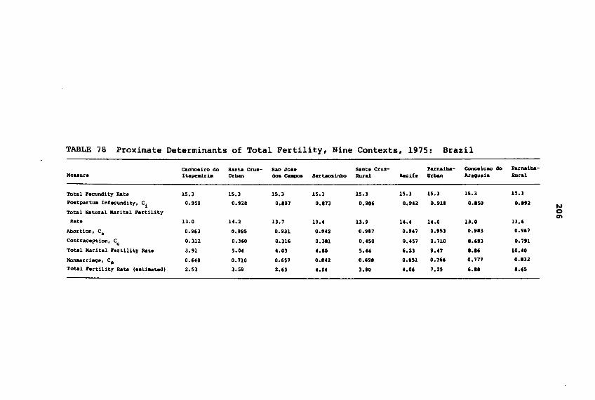
TABLE 78 Proximate Determinants of Total Fertility, Nine Contexts, 1975: Brazil

cachoeiro do Santa Crua- SAo Jo•• SAnta Ceu.- Parnaiba- Conce icAO do Parnaiba-Me••ute Ita~lr1. Urban clotI ca.pos llertaodnbo bral Recife Urban Arll9ueie Rural

Total Pecundity Rate 15.3 15.3 15.3 15.3 15.3 15.3 15.3 15.3 15.3

Poatpartua Infecundity. Ci 0.950 0.928 0.897 0.873 0.906 0.9'2 0.911 O.ISO 0.112

NTotal lIatural Marital Pertility 0

enRate 13.0 14.2 13.7 13•• 13.9 14 •• 14.0 13.0 13.6

Abortion, c. 0.963 0.985 0.931 0.9U 0.987 0.9'7 0.953 0.913 0.967

Contraception, Cc 0.312 0.360 0.316 0.311 0 ••50 0 ••57 0.710 0.613 0.711

Total Marital Pertility Rate 3.91 5.0. •• 03 •• 80 5." 6.23 9 ••7 1.16 10••0

NonaarriaCje, c. 0.U8 0.710 0.657 0.U2 0.698 0.651 0.766 0.717 0.132

Total Pertility Rate (eati_ted) 2.53 3.58 2.65 •• 0. 3.10 •• 06 7.25 6.18 1.65

207

to changing patterns of contraceptive use: increasedprevalence, coupled with the use of more effective methods(the pill and sterilization). Among the other proximatedeterminants of marital fertility, postpartum infecund­ability has relatively little impact in Brazil, where thepractice of breastfeeding is quite limited, abortion,shown in both data sets to be increasing, is neverthelessan indeterminate factor because of the usual data-gather­ing problems. Finally, both analyses point to a combina­tion of factors--changes in relative income, increasededucational attainment, and increased female labor forceparticipation--as the main socioeconomic determinant ofBrazil's changing patterns of contraceptive use: thesefactors are associated with increased desires for consumerdurables, the diffusion of information on family-sizelimitation, and therefore an increase in conscious fer­tility control.

NOTES

1 The relationship between income and fertility levelsis examined for the nine NIHR local contexts in Part IIof this report.2 Por a further discussion of the tyPOlogy used, see theAppendix. See also Lopes, (1975), Paria (1975), andSinger (1975).3 These case studies, which have already been conductedin the nine areas, can be found in the series Bstudos dePopulacao, CBBRAP, 1975-81, Sao Paulo.4 The justification for eliminating the usual age limitscan be found in Berquo (1973).5 When a member of the household group had any kind ofmarital union, previously or currently, and was under 18,he or she was also considered a candidate for sampling.6 See internal document prepared for the Project byPatarra (1976).7 Considering up to three as the maximum number ofunions, since a negligible fraction surpassed that number.8 Until November 1981, when the legal minimum wage was8,464 cruzeiros in Sao Paulo state, the cost of a civilmarriage was 1,650 cruzeiros, in Pernambuco (Northeast),these figures were 7,128 and 1,500 cruzeiros,respectively.9 Divorce was made legal in 1978, and with it came thepossibility of new legal unions.10 CBBRAP is at present conducting a study of themigrations affecting the NIHR.11 On this subject, see Brazil (1971-1980).12 These values refer to a subsample of about 100 womenfrom each context who had at least one child born alivein the last 5 years.13 Legal minimum wage limits in force at the time of thesurvey: Santa Cruz-Urban, $603.60 cruzerios, Sao Josedos Campos, $532.80 cruzerios, Cachoeiro do Itapemirim,$655.20 cruzerios, Parnaiba-Urban, $544.80 cruzerios,Recife, $602.40 cruzerios.

208

APPENDIX

TBB NID CONTEXTS

PARNAIBA*

Prom the nineteenth century onward, Parnaiba was the maincommercial entrepot for imports and exports in a primary­exporting economy (initially based on meat, and later onextractive products). Not only has it undergone the fluc­tuations and, finally, decline that are inherent in sucheconomies, but it has also in recent decades been edgedout of the main transportation and trading system by theincreasing dominance of road over river and sea transpor­tation. Beginning in the 1950s, this twofold process ledto a major change in the region's economy, which entereda phase of stagnation. Nevertheless, the municipalityretains the character of an extremely simple primary­exporting model, rooted in a peasantry that is practicallyunaffected by mercantile relations.

The 1970 data for the rural zone of Parnaiba depict alandowning structure in which the large estates, or lati­fundios, are of little commercial importance but arelinked to a broadly based peasant agriculture.

The importance of peasant activities in this munici­pality is reflected in its agrarian structure, which canbe seen in the distribution of land. In 1970, more than80 percent of establishments (those under 5 hectares)occupied less than 5 percent of the area exploited bytenants and sharecroppers. Less than 1 percent (22

*Summarized by Maria Lucia Indjaian, from a text by MariaAndrea Loyola based on papers by Lopes and Brandt (1978).

209

210

establishments with over 50 hectares) represented almosthalf the total area.

Half the value of agricultural and livestock-breedingactivities is attributable to farming and characteristic­ally commercial activities, just under one-third to animalhusbandry, and 12 percent to products of plant extraction.Cultivated areas are saall on average, with four basicproducts (rice, beans, cassava, and corn) representing 82percent of the municipality's agricultural production.The main commercial products are carnauba wax and cattle.A few establishments report some peraanent crop productionof a more commercial nature (banana, coconut, cashew, andmango), representing 8 percent of the overall value ofagricultural production. Rice is the only widespreadcommercial commodity whose production can be characterizedas peasant, its cultivation is aimed at obtaining a mone­tary supplement, and is in this way equivalent to the saleof leftovers from the grower's own consumption, seasonalemployment, or craft activities.

The most widespread labor relation in the area issharecropping. Ground rent varies depending on whetherthe land is handed over to the farmer already prepared forplanting, and whether the owner supplies the seed, it mayconsist of a half, a third, or a quarter share of produc­tion. The most common case is payment of the ground rentalone in the form of a quarter share, this kind of tenant,known as a rendeiro, often does not live on the land inquestion, which is usually let to him for 2 years. Hedepends in many ways on the landowner, who represents theonly channel for obtaining bank credit and even suppliesof foodstuffs. The sale of products grown on the landwill also depend on the landowner since they are oftensold ·on paper,· that is, as a future harvest. Althoughthis dependence aay vary in degree, it restricts thealternatives of the great majority who possess neitherland nor the conditions to acquire it. Another kind oftenant, the agregado*, usually lives on the estate and hasthe owner's permission to cultivate a small plot. Inreturn, he provides payment in the form of services, whichmayor may not be of an economic nature.

*Agregado: a term usually applied to one who lives on alarge estate_and has the owner's permission to cultivatea small plot in return for payment in the form of ser­vices (which mayor may not be economic in nature).

211

Parnaiba's urban economy is closely tied to this peas­ant economy. As in the past, the main roots of the urbaneconomy are in the ~rciali.ationof extractive pro­ducts. Of these, the most i~rtant is (and has beensince the beginning of the century) carnauba wax, prac­tically 100 percent of which is exported. In 1970, thevalue of foreign exports, consisting of carnauba wax andjaborandi, represented 90 percent of the total econoaicoutput. The babassu nut is distributed to the domestic.arket. At the present tille, while the town acts as areception center for products of plant extraction, it alsocontains a aodest aanufacturing sector. It reaains aservice center and a pole of demographic attraction. Itsmedical facilities are used by other .unicipalities 100lea away or more (BOIIle even in neighboring Maranhao andCeara), while its ~rcial establishments often servemore distant townships. Despite the weakening of itseconomy, the town continues to be the focus of ongoingrural-urban migration, and over the last decade, itsgrowth has increased. Bowever, this is probably attri­butable more to the stagnation of the rural economy thanto any dynamism in urban activities. In 1970, the urbanarea contained 60.87 percent of the popUlation, 25 percentof this population was not native to the municipality,having migrated aainly from Ceara (42.25 percent) andMaranhao (28.60 percent).

The 1970 Demographic Census showed that 35.1 percentof occupied persons worked in the secondary sector and62.4 percent in the tertiary. The 1970 Industrial Censusreported the existence of 114 industrial establishments,which absorbed 589 persons. If this number is subtractedfrom the total of 3,237 persons habitually occupied inmanufacturing activities according to the DemographicCensus, that leaves 2,648 persons involved in occasionalor irregular activities. This would seem to represent thereserve labor available to the town's industry for sea­sonal variations and turnover. The increase in the numberof persons engaged in manufacturing activities (21 per­cent) signifies a proliferation of domestic or autonomouscraft production rather than a growth of industry. Thereare only three industrial enterprises with more than 100employees (Vegetex, Morais e Cia., and Tropical de Alimen­tos). Most of those occupied in the manufacturing sector,according to demographic censuses, work in craft andrepair activities, as well.as in civil construction,which is in fact mostly repr~sented by craft activities.

212

The employment situation for ~rce is similar tothat for the industrial sector. The 1970 Commercial Cen­sus registered 1,025 wholesale and retail establishmentsemploying 1,824 persons. The Demographic Census showedthat 2,751 persons were habitually engaged in commercialactivities. This discrepancy can be explained primarilyby the seasonal nature of agriculture and extraction:trading in goods fluctuates with agricultural supply, andjob opportunities vary as a result. It is probable that,as with industry, this seasonal variation entails modifi­cations in the size of the autonomous sector, rather thana variation in demand for manpower. At present, Parnaibacan be seen as undergoing a rapid increase in the numbersof people occupied as ·autonomous· or self-employed inter­mediaries in the circulation of commodities. Of the 1,824persons registered by the Commercial census, the Demo­graphic Census classed 1,725 as being in this category.As regards local subsistence products, contrary to whatmight be expected of an economy based on small autonomousproduction, direct exchange does not predominate, but amultiple circuit based on buying and selling operations.As regards consumer products i~rted from other regions,the situation is more complex: although there are someWholesale firma, most of the large retail establishmentsseem to prefer to purchase their goods directly from lar­ger markets, and to this end have representatives in orsend buyers to Fortaleza, Rio, and Sao Paulo.

The low rates of pay common to several categories ofemployees and autonomous workers explains why they mustresort to a combination of agricultural, extractive,craft, industrial, and commercial activities to ensure theminimum earnings needed for survival. In 1970, 47.8 per­cent of those occupied in industry earned less than $100cruzerios (which then represented 80 percent of the legalminimum wage for the region). Among these workers, thatproportion was greater for employees (49.9 percent), andless for autonomous workers (47.4 percent), and those incommerce (47.2 percent). In the service sector, the cor­responding figures were 84.5 percent for employees and 74percent for autonomous workers.

The public sector is a major factor accounting foremployment levels in Parnaiba. The pace of public workshas a considerable influence on variations in job levels,while welfare and government health service agencies seemto be responsible for much of the municipality's monetary

. income. This is why a situation characterized by theexistence of large numbers of unemployed workers can con-

213

tinue, and vhy a large part of local c~rce can survive.In 1970, 6,720 of the total urban labor force of 15,052persons vere calculated to have been laid off for healthor other reasons according to the books kept at the Par­naiba branch of the IMPS (Instituto Macional de Previ­dencia Social--the governmental agency in charge of socialsecurity and the health services). Given the stagnationof the region's productive activities, it can be seen thatauch of the .cnetary circulation that enables small ca.­merce to survive in Parnaiba is injected by the IMPS, andsecondarily by the I'URlUJRAL (Rural WOrkers' Welfare Fund).The employaent situation vill be significantly alteredonly if there are even greater injections of governmentresources than those currently maintaining an active localmarket.

A summary of the main demographic indicators forParnaiba for the period 1940-70 is presented in Table A.l

CACBOEIRO DE ITAPEMIRIM*

The growth of the coffee trade vas the main factor in theoccupation of the territory now comprising the municipal­ity of Cachoeiro de Itapeairim and its surroundings, inthe south of Espirito Santo state. Settlement began in ,the early 1700s as a result of the hunt for gold in thecastelo mines and the setting up of the first sugar millsalong the banks of the River Itapemirim, however, it wasnot until the middle of the nineteenth century that: theexpansion of the coffee trade in the states of Minas andRio generated a definitive settlement of the EspiritoSanto tablelands, where Cachoeiro de Itapemirim lies.This period was also decisive in reinforcing the strategicposition occupied by Cachoeiro de Itapemirim since itsfoundation as a polarizing center for both the economicactivities and communications in the south of the state.The coffee trade brought the Leopoldina railroad as faras Cachoeiro, which thus became an entrepot for the entireregion's production on its way to the port of Rio de Jan­eiro, via Cachoeiro-Campos.

When the coffee trade began to decline, its place wastaken by livestock breeding, mostly of dairy cattle.Cachoeiro was also to be a nucleus for the dairy

*Summary by Sales (1979).

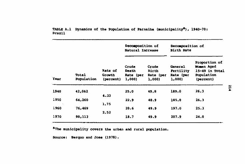
TABLE A.l Dynamics of the Population of Parnaiba (aunicipalityB), 1940-70:Brazil

Deea.position of oeco.position ofNatural Increase Birth Rate

Proportion ofCrude Crude General wo.en Aged

Rate of Death Birth Pertility 15-49 in TotalTotal Growth Rate (per Rate (per Rate (per Population

Year Population (percent) 1,000) 1,000) 1,000) (percent)

N~

1940 42,062 25.0 49.8 189.0 26.3 •4.33

1950 64,260 22.9 48.9 185.0 26.31.75

1960 76,469 20.6 49.9 197.0 25.32.52

1970 98,113 18.7 49.9 207.9 24.0

aThe municipality covers the urban and rural population.

Source: Berquo and Jose (1978).

215

production of the state's southern region, particularlyafter the founding of the cachoeiro de Itapemirim DairyCooperative in the 1940s and continuing to the present,when it absorbs the production from 18 neighboring munici­palities. The major consequence of this shift to dairycattle breeding is shown by cachoeiro's declining ruralpopulation, which from 1950 to 1970 fell from 53,701 to42,903, this represents a drop from 66.2 percent to 40.1percent of the municipality's total population. Its urbanpopulation, however, has been constantly growing: in1970, it reached 64,219, or 59.9 percent of the total,thus overtaking the rural population in relative terms.

This growth in cachoeiro's urban population is cer­tainly due mainly to the influx of aigrants attracted tothe town as the center of economic activities in theentire southern region of the state. However, this hasnot been the only result of the shift of population outof the municipality's rural areas. This migration hasvery probably reached not only cachoeiro, but also, andabove all, other rural areas in the same state or evenother states with an emerging agricultural frontier, infact, most of those who have migrated to the town ofcachoeiro have come from neighboring towns. Some datafrom field observation and secondary sources support thishypothesis. First, the main labor relation in the localcoffee plantations is the half-share sharecropping system,with a predominance of small producers. This leads theproducers naturally to look for other agricultural fron­tier regions when their own plantations undergo a crisis,prior to the decline in the coffee plantations, this hadalready been observed in the migration of small producersfrom the south to the central region of the state. Sec­ond, the municipality as a whole had a negative migratorybalance for 1960-70. Given the urbanization levelobserved for the municipality during the same decade, itis probable that this balance would have been positive ifa large proportion of those who emigrated from the coun­tryside had gone directly to the town of Cachoeiro.

The initial industrial thrust in Cachoeiro at thebeginning of the century was significant~r the laterconsolidation of urban society there, as well as for itsrecent industrial growth, still based mainly on theexploitation of the municipality's natural resources.Although no quantitative data are available for the yearsfollowing 1970, it seems undeniable that the town hasundergone its most significant growth over the last 10years because of the expansion of its dynamic industrial

216

sector and the resulting increase in cca.erce and servicesin general. The influx of immigrants to the town can beseen in the expansion of the urban site itself, which hasbegun spreading out along the banks of the River Itape­mirim toward the hills around the town. There has beenintense civil construction work over the last 10 years,above all in the building of new housing estates through­out the town's outskirts.

Industrial Census data show a degree of stabilizationin C.choeiro's industrial sector between 1940 and 1960,from then up to 1970, there was a substantial growth bothin the number of establishments and employees, and in thevalue of aanufacturing operations. Of the various kindsof industry, those which grew most over this period werethe extraction and production of nonmetallic minerals, thebasic raw aaterial in this field comes from the reservesof limestone and marble located in the municipality nearthe town of Cachoeiro. The largest and most diversifiedmarble and granite producers, however, began operationsor expanded out of already existing marble and granitecutting workshops in the late 1960s and early 1970s.Between 1970 (date of the last census) and 1979, when thefield survey was carried out, the number of firms in thissector decreased (from 80 to 4S establishments), while atthe same time the number of employees substantially in­creased (from 1,214 to 2,100). This would seem to indi­cate that during this period, the industrial sector under­went continuous vertical expansion, with the firmsinvolved growing, diversifying production, and absorbingother existing workshops.

Along with this industrial sector, made up mostly ofmedium and large factories engaged primarily in exportingtheir products, Cachoeiro also has a large number of smallfactories, most of which are engaged in supplying localconsumer needs. The great majority of industrialists arenative to the municipality, while many of its large-scaleenterprises arose as a result of individual initiative.The latter managed to expand their businesses into largefactories, such as the present-day I~apoa de Calcados(footwear), or even local empires, such as the ItapemirimGroup, whose main business is long-distance passengertransport, but whose activities also include a whole rangeof both service and industrial undertakings.

A summary of the main demographic indicators forCachoeiro de Itapermirin for the period 1940-70 ispresented in Table A.2.

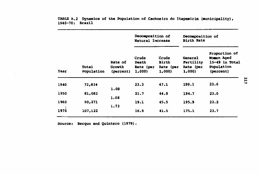
TABLE A.2 Dynamics of the Population of Cachoeiro do ItapeJllirim (aunicipal1ty),1940-10: Brazil

Decomposition of Decomposition ofNatural Increase Birth Rate

Proportion ofCrude Crude General we.en Aged

Rate of Death Birth Fertility 15-49 in TotalTotal Growth Rate (per Rate (per Rate (per Population

Year Population (percent) 1,000) 1,000) 1,000) (percent)

N....1940 12,834 23.3 41.1 199.1 23.6

...,1.08

1950 81,082 21.1 44.9 194.1 23.01.08

1960 90,211 19.1 45.5 195.9 23.2

19161.13

101,122 16.9 41.5 115.1 23.1

Source: Berquo and Quintero (1919).

218

SAO JOSE DOS CAMPOS*

Within the framework selected by the NID, Sao Jose dosCampos represents the case of modern Brazilian capitalismpowered by the forces of big oligopoly capital. Like theother towns in the Vale do Paraiba region, until the earlyyears of the present century, Sao Jose had an economybased on coffee planting. Unlike the other towns, how­ever, it did not slump when the coffee axis shifted to thewestern part af Sao Paulo state, rather it developed byreplacing coffee partly with semisubsistence activitiesand partly with livestock and dairy cattle breeding. Atthe same tiae, being a point of rail, and later road,intersection, it served as an entrepot for goods beingtransported from the large urban centers to the coastalports. It was in the 1950s, and especially in the 1960s,that Sao Jose began to take on the features of a modernBrazilian capitalist development because of the enormousindustrial boom that took place at this time. This boominvolved an industrialization process based on large-scaleenterprise, above all, it was a -modern- process in thatit was based on the expansion of oligopolies, or the so­called multinationals.

The distinctive marks of this process can be seen bothin the forms of economic organization that arose and inthe structure of local society: since industrializationwas based on the investments of large firms with headoffices outside the area, it operated through so-called-organizational policies- implemented by employees oper­ating on site (executives, managers, personnel heads,technicians, and engineers). At the same time, the pro­cess of industrialization and modernization formed theworkers into the -..sses.- This vas in fact a caricature,however, for they kept one foot in their past as migrantsand the other foot in the system of aspirations, whichsuffered drastic changes in the space of a few years.

Along with these characteristics, there arose an inter­mediary of great strength--the government and its agen­cies, and the weight of its -modernizing bureaucracy.­Government action contributed to economic growth from 1950onward, when the Centro Tecnico da Aeronautica (Air ForceTechnical Center) was set up. This was initially made upof technical and aeronautical engineering schools, but

*Summary by Maria Lucia Indjaian, based on Cardoso (1975).

219

later developed the nuclei of an aeronautics industry. Afurther contribution now being ..de by the state is theinstallation of huge facilities belonging to Petrobras(the state oil monopoly) for the construction ofrefineries.

Fra. 1960 onward, moreover, Sao Jose saw a change inthe pattern of its population dynamics. In 1960, therewere 76,997 inhabitants, a figure which rose to 148,332by 1970, of the latter, 74,395 were born outside the auni­cipality, and 94.2 percent of these were located in theurban area. Most of the aigrants in the local populationwere of Brazilian nationality, the aajority fra. thestates of Sao Paulo (48.94 percent) and Minas Gerais(37.09 percent). There were 2,651 foreigners (2 percentof the population), the same proportion as had been regis­tered for 1920, 1940, and 1950. As regards the urban orrural origins of the migrants, the available data showthat around 23,000 persons fra. the rural area werepresent in the urban area in 1970, this suggests that therural area aust have had little capacity to absorbworkers. In 1940, the rural population represented 63.5percent of the total population, falling to 11 percent in1970.

The degree of change undergone by the municipality'sproductive structure is reflected in its employment struc­ture. There has been a rapid decrease in the economicallyactive population in the primary sector, in 1940, itrepresented 60.86 percent of the labor force, and by 1973,it had been reduced to 2 percent. At the same t1Jle, therewas an increase in the secondary sector, which by 1973comprised 51 percent of the labor force, the re..ining 47percent was distributed among the commercial and servicesector (24.5 percent), public administration (11 percent),autonomous workers (11 percent), and others (0.3 percent).Meanwhile, women's participation in the labor forceincreased considerably: it grew in the tertiary sectorto 68.69 percent, where it was concentrated in individualconsumer services (39.96 percent) and others, although itlost relative importance in the primary (1.89 percent) andsecondary (29.42 percent) sectors.

These data indicate the proportionally greater increasein individual consumer services than in production ser­vices for the years after 1950 in Sao Jose. It is truethat the collective services sector also grew (education,police, health, etc.), indeed, for the latest intercensalinterval, this sector grew more than individual consumerservices. Even so, the number of domestic servants,

220

chauffeurs, snack bars, and so on greatly increased alongwith the so-called -.cdernization- caused by industrialgrowth. This shows in turn that Sao Jose is no exceptionto the occupational pattern created by the prevailingstyle of dependent capitalist society. In parallel, therewas an expansion in tertiary social areas (along with thestate bureaucracy), and social consumer services continuedto expand.

As regards wage distribution in 1970, in general, whitecollar employ... earned twice as .uch as workers, althoughthis gap was greater in some industries than in others.There was also a strong average differentiation amongwages within the various industries for both white andblue collar workers. Those industries with the highestpay for blue collar workers were chemicals and transpor­tation materials, together, those industries absorbed 37percent of occupied blue collar workers in Sao Jose, andthus forced the average wage upward. On the other hand,32 percent of blue collar workers earned less than halfthe average wage of all workers in the two industriesreferred to above, the corresponding figure for foodstuffsor metallurgy is 25 percent. Despite these wage differ­entials, however, the population's living standard did notmove beyond a -relative poverty horizon.-

As for rural economic activity, until 1960, the -abso­lute population level- remained steady, although it slowedin some periods. This activity comprised mainly cultiva­tion of rice, Irish potatoes, and sugarcane (especiallyfor fodder). There was also livestock (mainly dairy cat­tle) and poultry breeding, the latter, along with marketgardening, was intensified through use of the low-lyingland along the River Parnaiba. Dairy production and live­stock breeding were not adversely affected by the indus­trial boom, on the contrary, they even increased after1950, despite the loss of rural population. This suggeststhat resources were used to greater advantage and thatproduction was focused in large-scale agricultural enter­prises.

A summary of the main demographic indicators for SaoJose dos campos for the period 1940-70 is presented inTable A.3.

CONCElCAO DO ARAGUAIA*

Conceicao do Araguaia was founded in 1897 as a combinedcatechistic mission and hinterland settlement. Over the

*Summary by Maria Lucia Indjaian from Ianni (1978).

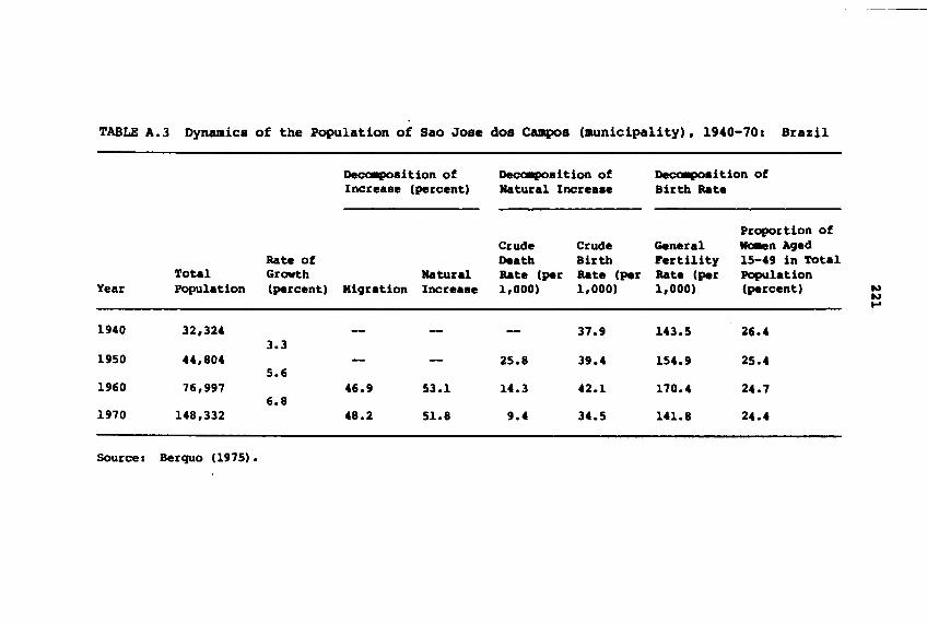
TABLE A.3 Dynamics of the Population of Sao Jose dos campos (aunicipality), 1940-70: Brazil

~.ition of ~.ition of ~ition ofIncrea.e (percent) Batura1 Increa.e Birth Rate

Proportion ofCrude Crude General wc.en Aged

Rate of Death Birth Fertility 15-49 in TotalTotal Growth Batura1 Rate (per Rate (per Rate (per Population

Year Population (percent) Migration Increa.e 1,000) 1,000) 1,000) (percent) NNI-'

1940 32,324 - -- -- 37.9 143.5 26.43.3

1950 44,804 - -- 25.8 39.4 154.9 25.45.6

1960 76,997 46.9 53.1 14.3 42.1 170.4 24.76.8

1970 148,332 48.2 51.8 9.4 34.5 141.8 24.4

Source: Berquo (1975).

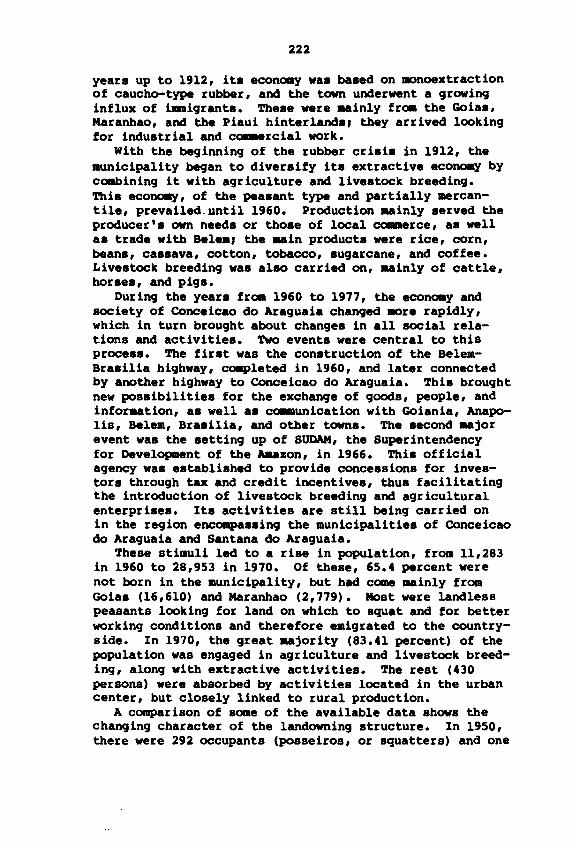
222

years up to 1912, its eco~ was based on monoextractionof caucho-type rubber, and the town underwent a growinginflux of immigrants. These were aainly from the Goias,Maranhao, and the Piaui hinterlands, they arrived lookingfor industrial and cem-ercial work.

With the beginning of the rubber crisis in 1912, theaunicipality began to diversify its extractive eco~ bycombining it with agriculture and livestock breeding.This econoay, of the peasant type and partially mercan­tile, prevailed-until 1960. Production aainly served theproducer's own needs or those of local commerce, as wellas trade with Bel••, the aain products were rice, corn,beans, cassava, cotton, tobacco, sugarcane, and coffee.Livestock breeding was also carried on, aainly of cattle,horses, and pigs.

During the years from 1960 to 1977, the eco~ andsociety of Conceicao do Araguaia changed more rapidly,which in turn brought about changes in all social rela­tions and activities. Two events were central to thisprocess. The first was the construction of the Belem­Brasilia highway, ca.pleted in 1960, and later connectedby another highway to Conceicao do Araguaia. This broughtnew possibilities for the exchange of goods, people, andinforaation, as well as ca.munication with Goiania, Anapo­lis, Belem, Brasilia, and other towns. The second aajorevent was the setting up of SUDAM, the Superintendencyfor Development of the Aaazon, in 1966. This officialagency was established to provide concessions for inves­tors through tax and credit incentives, thus facilitatingthe introduction of livestock breeding and agriculturalenterprises. Its activities are still being carried onin the region encc.passing the municipalities of Conceicaodo Araguaia and Santana do Araguaia.

These stimuli led to a rise in population, from 11,283in 1960 to 28,953 in 1970. Of these, 65.4 percent werenot born in the municipality, but had come mainly fromGoias (16,610) and Maranhao (2,779). Most were landlesspeasants looking for land on which to squat and for betterworking conditions and therefore emigrated to the country­side. In 1970, the great aajority (83.41 percent) of thepopulation was engaged in agriculture and livestock breed­ing, along with extractive activities. The rest (430persons) were absorbed by activities located in the urbancenter, but closely linked to rural production.

A comparison of some of the available data shows thechanging character of the landowning structure. In 1950,there were 292 occupants (posseiros, or squatters) and one

223

landowner (big farMr) with control of land in the 81ni­cipality. The occupant. were re.pon.ible for about 96percent of rural establi.n.ent. and occupied over 91 per­cent of the land involved. In 1970, the 2,136 occupant.accounted for over 95 percent of rUfal e.tabli.n.ent., butoccupied only 43.64 percent of the land, at the .aIIe time,there were 100 landowner., who accounted for 4.46 percentof rural e.tabli.n.ent. and occupied 56.33 percent of theland.

According to data collected by IBGB (Brazilian Geo­de.ic. and Stati.tic. In.titut.), agricultural and liv.­stock production gr.w ov.rall in th. y.ars from 1960 to1970, and the nuaber of rural e.tabli.n.ent. ro.e from 982(1960) to 2,242 (1970). The ca.po.ition of the populationengaged in agriculture and liv••tock breeding in 1972clearly .bows thi. chang.. In 1972, IHCRA (National S.t­tleMnt and Agrarian Reform In.titut.) regi.t.red 857permanent wage worker. and 7,011 temporary worker.. Ofthese, the peao, or un.killed wage laborer (lIIO.tly ofmigrant origin, a. well a. a peasant in th. proc••• ofproletarianization), was the central figure in the foraa­tion and .xpansion of th. large agricultural enterpri••••Thus, it i. above all in the country.ide that th. bour­geoi.ie and proletariat were incr.a.ingly taking .hape.On the one hand, th.re were the landowners, the faz.n­deiros, and the .ntrepren.ur. or their agent., on theother, there were the rural laborer. and cowhand.. Along­side with the.e, th.re w.re the pea.ant nuclei of ...11­holders, squatter., and colono., all in a critical pha••of reorganization or dissolution.

This pea.antry, who.e eeono.y originally con.i.ted offamily labor and was at a very low technological level,and who produced aainly for their own consumption, beganto produce for selling on the urban aarket, where thedemand for agriCUltural and extractive products was con­stantly rising. Together with this growing articulationbetween the peasant economy and the aarket, the peasantwas increa.ingly dependent on a .upply of merchandi.e(both e.sential and superfluous) generated by indu.trialcapital. This dependency developed and led to a dissolu­tion of the peasant economy. A large nuaber of the pea.­ants were transformed into di.gui.ed wage-earner, orsimply proletarianized, others, longstanding or recentsquatters, managed to have their legal situation redefinedand thus received permission to occupy or even own theland, becoming colonos. According to INCRA, in 1971, 90percent of all rural e.tabli.n.ents were in the hands of

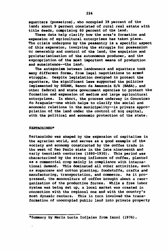
224

squatters (posseiros), who occupied 39 percent of theland, about 9 percent consisted of rural real estate withtitle deeds, cc.prising 60 percent of the land.

These data help clarify how the area's formation andexpansion of agricultural enterprises has taken place.The crisis undergone by the peaaantry is a specific aspectof this expansion, involving the struggle for possessionor ownership and control of the land, the expulsion andproletarianization of the autonomous producer, and theexpropr iation of the IIlOst iJIportant means of productionand subsistence--the land.

The antagoni.. between landowners and squatters tookany different for.., from legal negotiations to armedstruggle. Despite legislation designed to protect thesquatters, the significant laws supported the policiesimplemented by SUDAN, Banco da Allazonia S/A (BASA), andother federal and state government agencies to protect theformation and expansion of medium and large agriculturalenterprises. In short, the process underway in Conceicaodo Araguaia--one which helps to clarify the social andeconomic relations in the municipality--is private appro­priation of the land under the control of big capital,with the political and econoaic protection of the state.

SERTAOZINBO*

Sertaozinho was shaPed by the expansion of capitalism inthe agrarian world, and serves as a good example of thesociety and economy constructed by the coffee trade inthe west of Sao Paulo state in the late nineteenth andearly twentieth centuries (1880-1930). This period wascharacterized by the strong influence of coffee, plantedas a commercial crop mainly in compliance with interna­tional demand. This dominated all other activities, suchas sugarcane and cotton planting, foodstuffs, crafts andmanufacturing, transportation, and cOllllllerce. As it pro­gressed, the monoculture of coffee brought about a reor­ganization of the productive forces. While a free laborsystem was being set up, a local market was created inconnection with the regional one and with the country'smost dynamic centers. This in turn involved the trans­formation of unoccupied public land into private property

*Summary by Maria Lucia Indjaian from Ianni (1976).

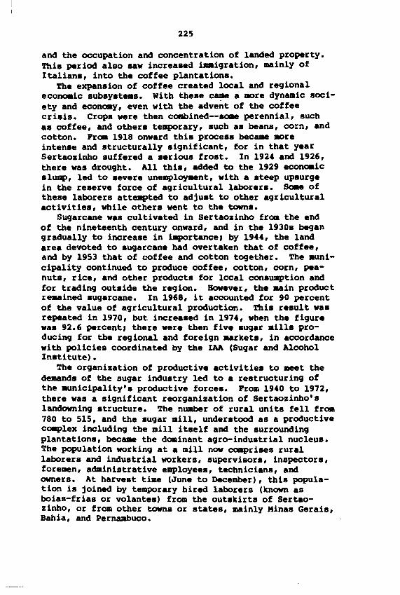
225

and the occupation and concentration of landed property.This period also sa" increased imaigration, mainly ofItalians, into the coffee plantations.

The expansion of coffee created local and regionaleconc.ic subsysteas. With these Calle a !lOre dynamic soci­ety and econoay, even with the advent of the coffeecrisis. Crops were then coabined--soge perennial, suchas coffee, and others teaporary, such as beans, corn, andcotton. PrOil 1918 on"ard this process bee.... !lOreintense and structurally significant, for in that yearSertaozinho suffered a serious frost. In 1924 and 1926,there "as drought. All this, added to the 1929 econc.icslump, led to severe unempl~nt, "ith a steep upsurgein the reserve force of agricultural laborers. SoRe ofthese laborers atteapted to adjust to other agriculturalactivities, while others went to the towns.

Sugarcane "as cultivated in Sertaozinho from the endof the nineteenth century on"ard, and in the 1930s begangradually to increase in iaportance, by 1944, the landarea devoted to sugarcane had overtaken that of coffee,and by 1953 that of coffee and cotton together. The auni­cipality continued to produce coffee, cotton, corn, pea­nuts, rice, and other products for lccal consumption andfor trading outside the region. However, the ..in productre..ined sugarcane. In 1968, it accounted for 90 percentof the value of agricultural production. This result "asrepeated in 1970, but increased in 1974, "hen the figure"as 92.6 percent, there "ere then five sugar aills pro­ducing for the regional and foreign ..rkets, in accordance"ith policies coordinated by the IAA (Sugar and AlcoholInstitute) •

The organization of productive activities to ...t thedemands of the sugar industry led to a restructuring ofthe aunicipality's productive forces. Prom 1940 to 1972,there "as a significant reorganization of Sertaozinho'slandowning structure. The nuaber of rural units fell from780 to 515, and the sugar aill, understood as a productiveca.plex including the mill itself and the surroundingplantations, beCalle the dominant agro-industrial nucleus.The population "orking at a mill now comprises rurallaborers and industrial workers, supervisors, inspectors,foremen, administrative employees, technicians, andowners. At harvest time (June to December), this popula­tion is joined by temporary hired laborers (known asboias-frias or volantes) from the outskirts of Sertao­zinho, or from other towns or states, mainly Minas Gerais,Bahia, and Pernaabuco.

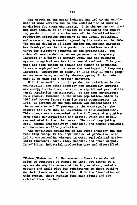
226

The growth of the sugar industry has led to the expul­sion of SODe workers and to the redefinition of workingconditions for those who remain. This change has occurrednot only because of an interest in increasing and improv­ing production, but also because of the formalization ofproduction relations according to the legal, political,and economic requirements iaposed by the state or the IAA.The social division of labor during and between harvestshas developed so that the production relations are dis­tinct for different seg-ents of the proletariat. Thecolonos* have tended to~ permanent or teaporarylaborers on a daily or monthly wage, and the colonatosystem in agriculture has thus been dissolved. This pro­cess has also tended to reduce the number of peraanentlaborers employed and increase the contingent of teaporarylaborers. According to INCRA, in 1972 only 11 rural prop­erties were being worked by sharecroppers, 21 in nuaber,only 10 of whom had a written contract.

With this modification in production relations in thecountryside, the sugar industry has indirectly impartednew energy to the town, to which a significant part of therural population has migrated. It has thus contributedto a gradual increase in the urban population, which by1960 had become larger than its rural counterparta in1940, 25 percent of the population was concentrated inthe urban area and 75 percent in the countryside, thefigures for 1970 show an inversion of this composition.This change was accc.panied by the influence of migrationfrom other aunicipalities and states, which was aainlyconcentrated in the urban area. The rural populationfell, bec... progressively urbanized, and became consumersof the urban world's production.

The continuous expansion of the sugar industry and theresulting change in the organization of production alsoled to corresponding changes in other agricultural activ­ities (soybeans, corn, rice, peanuts, and other crops).In addition, industrial production grew and diversified,

*Colono/Colonato: In Sertaozinbo, these terms do notrefer to squatters or owners of land, but rather to asystem whereby the owners of the big estates granted acottage and small plot for subsistence to those workingon their lands or at the mills. With the dissolution ofthis system, these workers lose such rights and areevicted from the land.

227

absorbing 60 percent of the .unicipality's economicallyactive population, in certain cases, this involved theprt.ary sector. Industrial establisn.ents increased innuaber from 33 in 1940 to 172 in 1973. In the same year,metallurgical and .echanical fir.., ~inly engaged inproduction and repair of aachinery and equipment for thesugar industry, emplO¥ed 50 percent of all persons occu­pied in the industrial sector. New capitalist productionpatterns became generalized through the influence of thesugar aarket, the relations of .utual dependence andantagonisa between tOwn and country, agr iculture andindustry, workers and bourgeoisie all changed as a result.

A su..ary of the aain de.agraphic indicators for Ser­taozinho for the period 1940-70 is presented in Table A.4.

SANTA CRUZ DO SOL*

The lands in the settlement of Santa Cruz do Sul wereoccupied from 1849 onward. In that year, 77-hectare plotswere distributed as an incentive to foreign i..igration,which was needed to aake up for the scarcity of manpower,especially in the field of agricultural exports, and topromote the free land system. The migratory influx toSanta Cruz do Sul steadily increased until the end of thenineteenth century and was .ostly made up of Germansettlers.

The economy of Santa Cruz was based fro. the start onfamily agricultural production for export. Its aain pro­duct was tobacco, but there were also lard, Paraguay tea,beans, and corn. Together with these activities, thisdevelopment of an export trade in agricultural productsled to an accumulation of capital, which in turn facili­tated the installation of production units along capital­ist lines. Prom 1918 on, .ost of the firms in the townwere engaged in processing agricultural products (dryingtobacco, refining lard) and preparing them for export asraw aaterials. This led to an expansion of tobacco­related activities and a decline in those related to pro­ducts sold on the hODe aarket, subsistence, or pig breed­ing, thus making the municipality's economy more and moredependent on a single product.

*Summary by Maria Lucia Indjaian, from Lima (n.d.) andOliveira (1975).

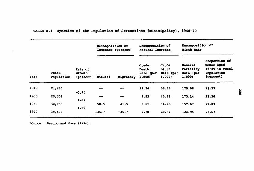
TABLE A.4 Dynamics of the Population of Sertaozinho (aunicipality), 1940-70

Decomposition of Decomposition of DecoIIpoaition ofIncrease (percent) Natural Increaae Birth Rate

Proportion ofCrude Crude General wo.en Aged

Rate of Death Birth Fertility 15-49 in TotalTotal Growth Rate (per Rate (per Rate (per Population

Year Population (percent) Natural Migratory 1,000) 1,000) 1,000) (percent)

1940 21,290 -- -- 19.34 39.88 179.08 22.27 w-0.45 w

C»1950 20,357 -- -- 9.53 40.28 173.14 23.26

4.871960 32,753 58.5 41.5 8.65 34.78 152.07 22.87

1.891970 39,496 135.7 -35.7 7.70 29.57 124.95 23.67

Source: Berquo and Jose (1976).

229

There was also a greater fragDentation of rural prop­erty, reaching a peak between 1920 and 1940. Over thisperiod, the average area of properties fell from 40 to26.93 hectares, while the number of establishments withbetween 1 and 20 hectares grew. This considerable reduc­tion in the size of properties meant that it was no longerpossible to maintain the system of dividing them up ac­cording to inheritance, thus sa.e owners' children wereforced off the land, to undergo a precess of proletarian­ization in later years when the town's industrializationwas unde r way.

The process of emigration from the rural zone, alreadyintense in the 1940s and 1950s, became .are so in laterdecades as the parceling out of property continued. Itwas also encouraged by the tobacco crisis since this pro­duct dominated the municipality's agricultural and indus­trial economy. The tobacco crisis was partly caused bythe federal government's inflationary policies from 1962onward, and partly by a failure to update production tech­niques. As a result, this aajor export l6st its aarketcompetitiveness. This in turn led to the introduction offoreign capital, which was gradually invested in the pur­chase of the existing tobacco factories.

The landowning structure of Santa Cruz do sul is char­acterized by a predominance of small agricultural estab­lishmentsz in 1970, the Agricultural Census registered8,226 establisn.ents in the aunicipality, absorbing 27,423persons. There are, however, no precise data on the num­ber of PeOple engaged in tobacco planting. The proportionof wage-earners is small (around 10 percent of the eco­nomically active population), as is the share of tenantfarmers, squatters, and occupants (around 8 percent). Themajority consists of smallholders (colonos) and membersof their families (82 percent), who are engaged in SUbsis­tence production, along with tobacco and soybean plantingand pig breeding.

These activities are carried on in the area where Ger­man settlers predominate, which is also the richest. Thenorthern part of the municipality, occupied mainly byItalians, has different features. Bere, properties arerelatively larger, the ground ia less even, and livestockbreeding thus predominates, along with Paraguay teaextraction. Wage labor is also common in this area.

Industrial activities are an extension of agriculture,eSPeCially tobacco processing and cigarette manufacturing.The 1970 Industrial Census registered 5,287 personsoccupied in industry, of whom 3,899 were in production.

230

Among these, the tobacco industry (including cigarettefactories and tobacco-processing plants) emplcyed 1,141persons as permanent workers. The processing plants aredirectly linked to the planters, they render technicalassistance, supplying fertilizers and insecticides, andfinance the construction of curing barns. Thus, theplanters are distinctly dependent on these processingfirmsl although there is no formal contract, any planterwho fails to sell his production to the firm that financedhim will stand little chance of receiving financial aidin the future.

The tobacco-processing firms employ few permanentworkers since their demand for labor increases 3-5 timesat the harvest peak (March-April). SOuza Cruz has 200permanent employees, but at harvest time this rises to1,000. No preference is shown to either sex in theemployment of harvest workers (usually it is 50 percentfor each), and workers may be either single or married.They work for the processors around 3-4 months every year.The rest of the year they are employed in civil construc­tion or do odd jobs. A few emigrate to Rio Pardo orCachoeira do Sul, where they work on the rice or wheatharvest, while some remain unemployed. The women usuallywork as domestic servants in private residences.

Of the large enterprises outside the tobacco industry,the most important are a meat packing plant and a rubbergoods factory. The remaining enterprises--mainly lumber­ing and the manufacture of furniture, perfume, and bev­erages--employ relatively few workers. In fact, there aremany small firms with few or no employees, on the basisof the census data, it can be assumed that most industrialestablishments employ on average less than 10 persons.

Along with industrial activities, Santa Cruz has smalland medium-sized commerce that serves the needs of themunicipality and its neighbors. Most of the largertradesmen are former tobacco entrepreneurs who, in thelate 1960s and early 1970s, were brought up by interna­tional groups. It is impossible to obtain a clear pictureof the occupational categories in commercial activitiesfrom the 1970 Commercial Census since it also includesinformation on industry. The 1960 census, however,clearly shows a predominance of proprietors and theirfamilies in commerce, mainly in the retail sector (39percent wage-earners), in contrast, wage-earners predomi­nated in wholesale commerce (76.7 percent). The servicesector also remained small, absorbing around 7 percent ofthe municipality's economically active population, of

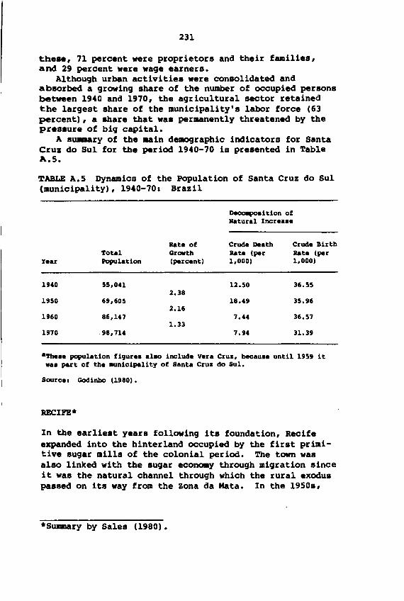
231

the.. , 71 percent were proprietors and their families,and 29 percent were wage earners.

Although urban activities were consolidated andabsorbed a growing share of the number of occupied personsbetween 1940 and 1970, the agricultural sector retainedthe largest share of the municipality's labor force (63percent), a share that was permanently threatened by thepressure of big capital.

A su.aary of the ..in d.-ographic indicators for SantaCruz do Sul for the period 1940-70 is presented in TableA.5.

TABLE A.5 Dynamics of the Population of Santa Cruz do sul(municipality), 1940-70: Brazil

DecoIIpodtion ofN.tur.1 Incr••••

Rate of Crud. De.th Crud. BirthTotal Growth Rate (per Rate (per

Ye.r Population (percent) 1,000) 1,000)

1940 55,041 12.50 36.552.38

1950 69,605 18.49 35.962.16

1960 86,147 7.44 36.571.33

1970 98,714 7.94 31.39

·The.e popu1.tion figure••1ao include Vera Crus, bec.u.e until 1959 it••• part of the aunicipa1ity of S.nt. Crus do Su1.

Source. Godinho (1980).

RECIFE*

In the earliest years following its foundation, Recifeexpanded into the hinterland occupied by the first primi­tive sugar mills of the colonial period. The town wasalso linked with the sugar econo.y through migration sinceit was the natural channel through which the rural exoduspassed on its way from the Zona da Nata. In the 1950s,

*Summary by Sales (1980).

232

when the population of the town of Recife most increased,the proportion of the migratory increase to the totalpopulation growth was nearly 50 percent. The few dataavailable point to the fact that these migrants came aboveall from the Zona da Mata, a hinterland region which inturn receives migratory currents of a temporary or perma­nent nature (the so-called coruabes from the Agresteregion) coming from regions even farther inland in thesame state.

The Zona da-Mata therefore for.. a green belt aroundRecife, as happens with other regional metropolises.However, it does not supply the town with foodstuffs--onlywith migrant population. ApParently, the structural con­ditions associated with changes in the sugar economy ledto this emigration from the sugar-producing region, mostof which empties into Recife. The urban problems gener­ated by this sizable influx of migrants can be seen aboveall in the proliferation of shanty-towns (locally knownas mocambos) in the waterlogged outskirts of the town.

The dynamics of interregional integration under thehegemony of the Center-SOuth and its process of indus­trialization resulted both in the intensification of com­merce and migration between regions and in the growth ofRecife after 1950. The integration of the Northeast intothe model of capital accumulation (whose hegemonic polewas located outside the region) led to the disorganizationof the agrarian and productive structure of the Recifehinterland and thus further encouraged migration into thetown. Recife's urban problems therefore became linked tothose of the region, which centered on the decline oflocal productive activities.

The same factors which account for migrations at themacro-structural level also account for the disorganiza­tion of certain industries. The introduction of manufac­tured goods from the Center-South was the main reason forthe closing down of certain branches of Recife's industry,in particular the textile industry. This helps to explainthe creation of SODBNE (Superintendency for Developmentof the Northeast) in 1959, with headquarters in Recife.The primary objective of this agency was to resolve theseproblems by revitalizing industry, creating jobs, anddiversifying production.

The appearance of SODBNE marked a new era in the lifeof the town of Recife, primarily because of the new dynam­ics of urban employment resulting from the industrialprojects implemented in the Northeast through tax incen­tives. In the 1960s, industry in the metropolitan area

233

received a new injection of resources. However, this infact led to an increase in manufacturing production ratherthan in the nuaber of jobs, indicating the iRPOrtance ofthe technological component in the industrialization ofthe Northeast under the auspices of SUDBNE. The effectof the reorganization of industry in the area on the laborforce can be seen in a drop in employment in the secondarysector in municipalities that traditionally housed a majorportion of the state's textile industry (Paulista andMoreno).

The greatest growth was in the tertiary sector, espe­cially in those branches where urban underemployment hadbeen heaviest. If the various census data are combinedwith the findings of anthropological investigations car­ried out in Greater Recife, the most salient recent fea­ture of the occupational structure in Recife's .etropoli­tan area that emerges is intense fluctuation in the laborforce between employment, unemployment, odd jobs, andvarious kinds of underemployment. Attention must also bepaid to the increasing importance of the so-called infor­mal sector in the economy as a whole, particularly duringthe post-SUDBHE period, one example would be small com­mercial establisn.ents, whose initial capital oftendepends on the small trader's position in the regularlabor market.

The conflicts between the intense population growth,the poor living conditions in the marshland shantytowns,and the rising value of urban land after 1960 led to a newkind of migratory movement--intrametropolitan aigration.This movement led to considerable population increases inthe 1960s in the municipalities of Olinda, Jaboatao, andSao Lourenco da Mata, which underwent a process of urbanexpansion as if they were outlying districts of Recifeitself.

A summary of the main demographic indicators forRecife for the period 1940-70 is presented in Table A.6.

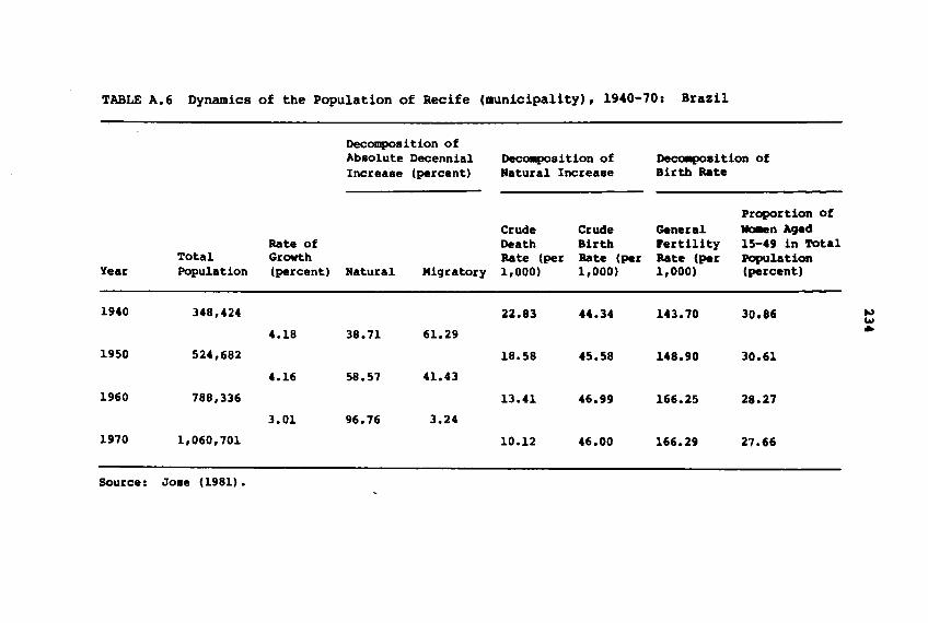
TABLE A.6 Dynamics of the Population of Recife (municipality), 1940-70: Brazil

Decomposition ofAbsolute Decennial ~sition of Deee-position ofIncrease (percent) Natural Increase Birth Rate

Proportion ofCrude Crude General wa.en Aged

Rate of Death Birth Fertility 15-49 in 'l'OtalTotal Growth Rate (per Rate (per Rate (per Population

Year Population (percent) Natural Migratory 1,000) 1,000) 1,000) (percent)

1940 348,424 22.83 44.34 143.70 30.86 ww

4.18 38.71 61.29 ..1950 524,682 18.58 45.58 148.90 30.61

4.16 58.57 41.43

1960 788,336 13.41 46.99 166.25 28.27

3.01 96.76 3.24

1970 1,060,701 10.12 46.00 166.29 27.66

Source: JOBe (1981).

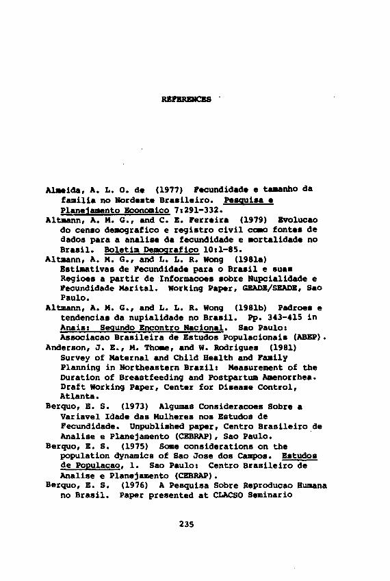
RBI'BRBIICBS .

AlMida, A. L. O. d. (1977) Pecundidad. e taaanho dafamilia no Nord.st. Brasileiro. Pesguisa.Planejamento Bconoaico 71291-332.

Altaann, A. M. G., and C. B. Perr.ira (1979) Bvolucaodo censo demoqrafico e registro civil ca.o font.s dedados para a anali•• da fecundidade e JIOrtalidad. noBrasil. Boleti. De!ografico 1011-85.

Altmann, A. M. G., and L. L. R. wong (1981a)Bstt.4tivas de Pecundidad. para 0 Brasil e suasRegioes a partir de ·Informacoes sobre Hupcialidade ePecundidade Marital. Working Paper, GBADB/SBADB, SaoPaulo.

Altmann, A. M. G., and L. L. R. Wong (1981b) Padroes etendencias da nupialidade no Brasil. pp. 343-415 inAnaisl Segundo Bncontro Hacional. Sao PaulolAssociacao Brasileira de Bstudos Populacionais (ABBP).

Anderson, J. B., M. ThOlle, andW. Rodrigues (1981)Survey of Maternal and Child Health and PamilyPlanning in Northeastern Brazill Measurement of theDuration of Breastfeeding and Postpartum Amenorrhea.Draft Working Paper, Center for Disease Control,Atlanta.

Berquo, B. S. (1973) Algumas Consideracoes Sobre aVariavel Idade das Mulheres nos Bstudos deFecundidade. Unpublished paper, Centro Brasileiro.deAnalise e Planejamento (CBBRAP), Sao Paulo.

Berquo, B. S. (1975) Some considerations on thepopulation dynamics of Sao Jose dos campos. Bstudosde Populacao, 1. Sao Paulol Centro Brasileiro deAnalise e Planejamento (CBBRAP).

Berquo, B. S. (1976) A Pesquisa Sobre Reproducao Humanano Brasil. Paper presented at CLACSO Seminario

235

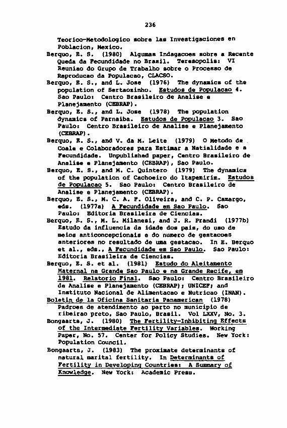
236

Teorico-Metodologico sobre las Investigaciones enPoblacion, Mexico.

Berquo, B. S. (1980) Algumas Indagacoes sobre a RecenteQueda da Fecundidade no Brasil. Teresopolis: VIReuniao do Grupo de Trabalho sobre 0 Processo deReproducao da Populacao, CLACSO.

Berquo, B. S., and L. Jose (1976) The dynamics of thepopulation of Sertaozinho. Bstudos de Papulacao 4.Sao Paulo: Centro Brasileiro de Analise ePlanejamento (CBBRAP).

Berquo, B. S., and L. Jose (1978) The populationdynamics of Parnaiba. Bstudos de Populacao 3. SaoPaulo: Centro Brasileiro de Analise e Planejamento(CBBRAP) •

Berquo, B. S., and V. da M. Leite (1979) 0 Metodo decoale e Colaboradores para Bsttmar a Natialidade e aFecundidade. Unpublished paper, Centro Brasileiro deAnalise e Planejamento (CEBRAP), Sao Paulo.

Berquo, B. S., and M. C. Quintero (1979) The dynamicsof the population of Cachoeiro do Itapemirim. Bstudosde Populacao 5. Sao Paulo: Centro Brasileiro deAnalise e Planejamento (CBBRAP).

Berquo, B. S., M. C. A. F. Oliveira, and C. P. Camargo,eds. (1977a) A Fecundidade em Sao Paulo. SaoPaulo: Editoria Brasileira de Ciencias.

Berquo, E. S., M. L. Milanesi, and J. R. Prandi (1977b)Estudo da influencia da idade dos pais, do uso demeios anticoncepcionais e do numero de gestacoesanteriores no resultado de uma gestacao. In E. Berquoet al., eds., A Fecundidade em Sao Paulo. Sao Paulo:Editoria Brasileira de Ciencias.

Berquo, E. S. et ale (1981) Estudo do AleitamentoMaternal na Grande Sao Paulo e na Grande Recife, em1981. Relatorio Final. Sao Paulo: Centro Brasileirode Analise e Planejamento (CEBRAP)J UNICEFJ andInstituto Nacional de Alimentacao e Nutricao (INAN).

Boletin de la Oficina Sanitaria Panamerican (1978)Padroes de atendimento ao parto no municipio deribeirao preto, Sao Paulo, Brasil. Vol LXXV, No.3.

Bongaarts, J. (1980) The Fertility-Inhibiting Effectsof the Intermediate Fertility Variables. WOrkingPaper, No. 57. Center for Policy Studies. New York:Population Council.

Bongaarts, J. (1983) The proximate determinants ofnatural marital fertility. In Determinants ofFertility in Developing Countries: A Summary ofKnowledge. New York: Academic Press.

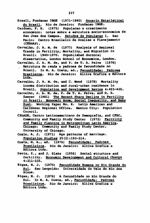
237

Brazil, Fundacao 18GB (1971-1980) Anuario Estatisticaldo Brasil. Rio de Janeiro: Fundacao 18GB.

Cardoso, F. H. (1975) Populacao e crescimentoeconomicol notas sobre a estrutura socio-economica deSao Jose dos Campos. Estudos de PoPulacao 1. SaoPaulo: Centro Brasileiro de Analise e Planejamento(CEBBAP) •

Carvalho, J. A. M. de (1973) Analysis of RegionalTrends in Fertility, Mortality, and Migration inBrazil: 1940-1970. Unpublished doctoraldissertation, London SChool of Economics, London.

Carvalho, J. A. M. de, and P. de T. A. Paiva (1976)Estrutura de renda e padroes de fecundidade noBrasil. In M. A. Costa, ed., Fecundidade: PadroesBrasileros. Rio de Janeiro: Altiva Grafica e EditoraLtda.

Carvalho, J. A. M. de, and C. WOOd (1978) Mortalityincome distribution and rural-urban residence inBrazil. Population and Develop!!nt Review 4:405-420.

Carvalho, J. A. M. de, P. de T. A. Paiva, and D. R.Sawyer (1981) The Recent Sharp Decline in Fertilityin Brazil: Economic soo., Social Inequality, and BabyBust. Working Paper No.8. Latin American andCaribbean Re9ional Office. Mexico City: populationCouncil.

CELADE, Centro Latinoamericano de Demografia, and CFSC,community and Family Study Center (1972) Fertilityand Family Planning in Metropolitan Latin America.Chicago: community and Family Study Center,University of Chicago.

Coale, A. J. (1971) Age patterns of marriage.Population Studies 25(2):193-214.

Costa, M. A., ed. (1976) Fecundidade: PadroesBrasileiros. Rio de Janeiro: Altiva Grafica eEditora Ltda.

Davis, K., and J. Blake (1956) Social structure andfertility. Economic Development and Cultural Change4:211-235.

Etges, N. J. (1975) Fecundidade Humana no Rio Grande.doSul. Sao Leopoldo: Universidade do Vale do Rio dosSinos.

Etges, N. J. (1976) A fecundidade no Rio Grande' doSul. In M. A. Costa, ed., Fecundidade: PadroesBrasileiros. Rio de Janeiro: Altiva Grafica eEditora Ltda.

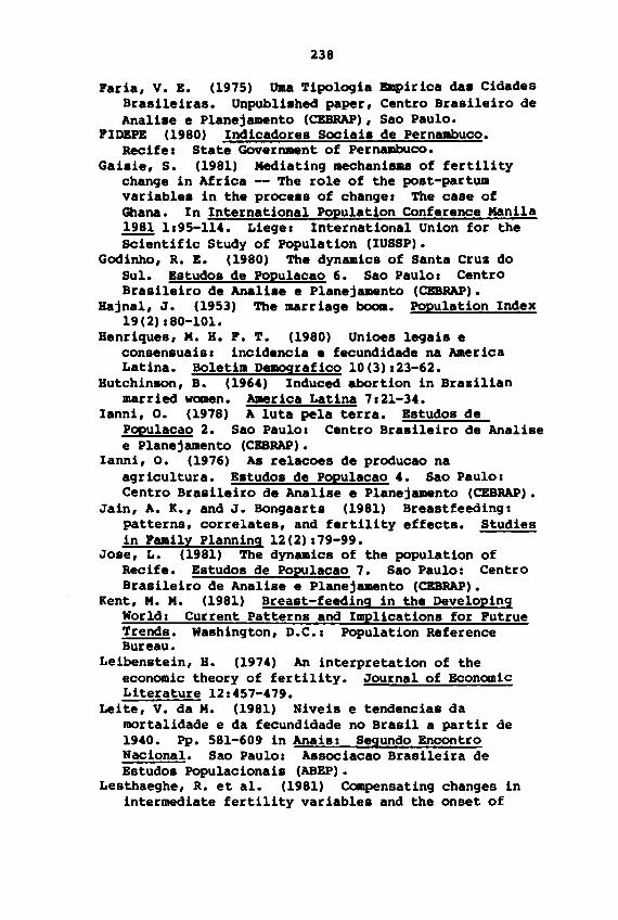
238

Faria, V. B. (1975) oaa Tipologia Bmpirica das CidadesBrasileiras. Unpublished paper, Centro Brasileiro deAnalise e Planejamento (CBBRAP), Sao Paulo.

FIDBPB (1980) Indicadores Sociais de Pernaabuco.Recife: State Gover~nt of Pernambuco.

Gaisie, S. (1981) Mediating mechani... of fertilitychange in Africa -- The role of the post-par twavariables in the process of change: The case ofGhana. In International Population Conference Manila1981 1:95-114. Liege: International Union for theSCientific Study of Population (IUSSP).

Godinho, R. B. (1980) The dynamics of Santa Cruz doSul. Bstudos de Populacao 6. Sao Paulo: CentroBrasileiro de Analise e Planejamento (CBBRAP).

Hajnal, J. (1953) The marriage boca. Population Index19(2) :80-101-

Henriques, M. H. F. T. (1980) Unioes legais econsensuais: incidencia e fecundidade na AmericaLatina. Boletim De!ografico 10(3):23-62.

Hutchinson, B. (1964) Induced abortion in Brazilianmarried wClIIIen. America Latina 7:21-34.

Ianni, o. (1978) A luta pela terra. Bstudos dePapulacao 2. Sao Paulo: Centro Brasileiro de Analisee Planejamento (CBBRAP).

Ianni, o. (1976) As relacoes de producao naagricultura. Estudos de Populacao 4. Sao Paulo:Centro Brasileiro de Analise e Planejamento (CEBRAP).

Jain, A. K., and J. Bongaarts (1981) Breastfeeding:patterns, correlates, and fertility effects. Studiesin Family Planning 12(2):79-99.

Jose, L. (1981) The dynamics of the population ofRecife. Estudos de PORUlacao 7. Sao Paulo: CentroBrasileiro de Analise e Planejamento (CEBRAP).

Kent, M. M. (1981) Breast-feeding in the DevelopingWorld: Current Patterns and Implications for FutrueTrends. Washington, D.C.: Population ReferenceBureau.

Leibenstein, H. (1974) An interpretation of theeconomic theory of fertility. Journal of EconomicLiterature 12:457-479.

Leite, V. da M. (1981) Niveis e tendencias damortalidade e da fecundidade no Brasil a partir de1940. pp. 581-609 in Anais: Segundo EncontroNacional. Sao Paulo: Associacao Brasileira deEstudos Populacionais (ABEP).

Lesthaeghe, R. et ale (1981) compensating changes inintermediate fertility variables and the onset of

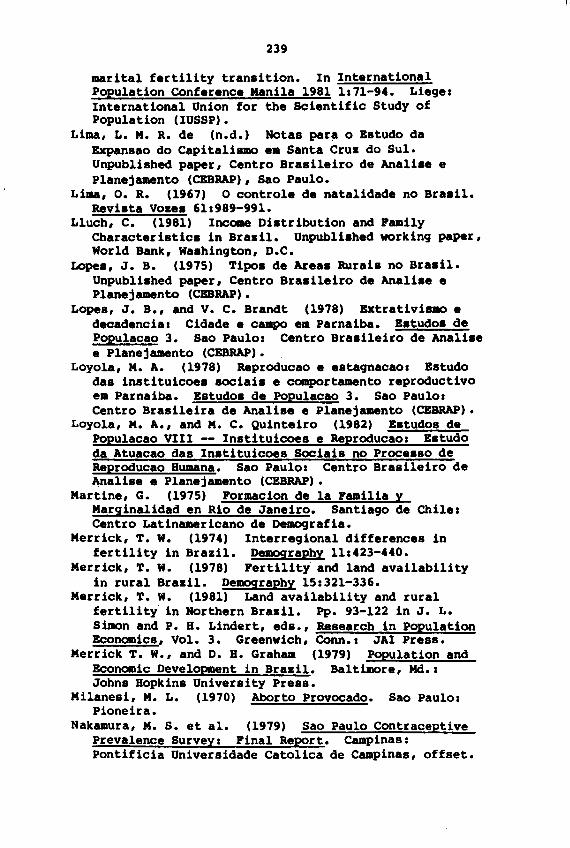
239

marital fertility transition. In InternationalPopulation Conference Manila 1981 1:71-94. Liege:International Union for the SCientific Study ofPopulation (IUSSP).

Lima, L. M. R. de (n.d.) Notas par~ 0 Estudo daExpansao do Capitalismo e. Santa Cruz do Sul.Unpublished paper, Centro Brasileiro de Analise ePlanejamento (CBBRAP), Sao Paulo.

Lima, O. R. (1967) 0 controle de natalidade no Brasil.Revista Vozes 61:989-991.

Lluch, C. (1981) Income Distribution and FamilyCharacteristics in Brazil. Unpublished working paper,World Bank, Washington, D.C.

Lopes, J. B. (1975) Tipos de Areas Rurais no Brasil.Unpublished paper, Centro Brasileiro de Analise ePlanejamento (CEBRAP).

Lopes, J. B., and V. C. Brandt (1978) ExtrativiUlO edecadencia: Cidade e campo e. Parnaiba. Estudos dePopulacao 3. Sao Paulo: Centro Brasileiro de Analisee Planejamento (CEBRAP).

Loyola, M. A. (1978) Reproducao e estagnacao: Estudodas instituicoes sociais e comportamento reproductivoe. Parnaiba. Estudos de Populacao 3. Sao Paulo:Centro Brasileira de Analise e Planejamento (CEBRAP).

Loyola, M. A., and M. C. Quinteiro (1982) Estudos dePopulacao VIII -- Instituicoes e Reproducao: Estudoda Atuacao das Instituicoes Sociais no Processo deReproducao Humana. Sao Paulo: Centro Brasileiro deAnalise e Planejamento (CEBRAP).

Martine, G. (1975) Formacion de la Familia yMarginalidad en Rio de Janeiro. Santiago de Chile:Centro Latinamericano de Demografia.

Merrick, T. W. (1974) Interregional differences infertility in Brazil. DemographY 11:423-440.

Merrick, T. W. (1978) Fertility and land availabilityin rural Brazil. Demography 15:321-336.

Merrick, T. W. (1981) Land availability and ruralfertility in Northern Brazil. pp. 93-122 in J. L.Simon and P. H. Lindert, eds., Research in PopulationEconomics, Vol. 3. Greenwich, Conn.: JAI Press.

Merrick T. W., and D. H. Graham (1979) Population andEconomic Development in Brazil. Baltimore, Md.:Johns Hopkins University Press.

Milanesi, M. L. (1970) Aborto Provocado. Sao Paulo:Pioneira.

Nakamura, M. S. et al. (1979) Sao Paulo ContraceptivePrevalence Survey: Final Report. Campinas:Pontificia Universidade Catolica de Campinas, offset.

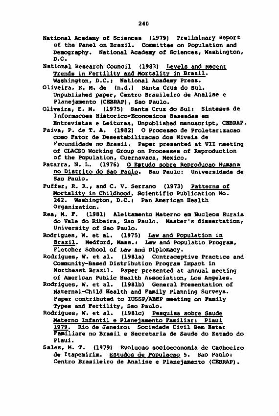
240

National Academy of SCiences (1979) Preliminary Reportof the Panel on Brazil. committee on Population andDemography. National Academy of SCiences, Washington,D.C.

National Research COUncil (1983) Levels and RecentTrends in Fertility and Mortality in Brazil.Washington, D.C.: National Academy Press.

Oliveira, E. M. de (n.d.) Santa Cruz do Sul.Unpublished paper, Centro Brasileiro de Analise ePlanejamento (CBBRAP), Sao Paulo.

Oliveira, E. M. (1975) Santa Cruz do Sul: Sinteses deInformacoe. Hi.torico-Bconomico. Baseadas emEntrevistas e Leituras, Unpublished manuscript, CBBRAP.

Paiva, P. de T. A. (1982) 0 Processo de Proletarizacaocomo Fator de Desestabilizacao dos Niveis deFecundidade no Brasil. Paper presented at VII meetingof CLACSO Working Group on Processes of Reproductionof the Population, Cuernavaca, Mexico.

Patarra, N. L. (1976) 0 E.tudo sobre Reproducao Humanano Distrito do Sao Paulo. Sao Paulo: Universidade deSao Paulo.

Puffer, R. R., and C. V. Serrano (1973) Patterns ofMortality in Childhood. SCientific Publication No.262. Washington, D.C.: Pan American HealthOrganization.

Rea, M. F. (1981) Aleitamento Materno em Nucleos Ruraisdo Vale do Ribeira, Sao Paulo. Master's dissertation,University of Sao Paulo.

Rodrigues, W. et ale (1975) Law and Population inBrazil. Medford, Mass.: Law and Populatio Program,Fletcher School of Law and Diplomacy.

Rodrigues, W. et ale (1981a) COntraceptive Practice andCOmmunity-Based Distribution Program Impact inNortheast Brazil. Paper presented at annual meetingof American Public Health Association, Los Angeles.

Rodrigues, W. et ale (1981b) General Presentation ofMaternal-Child Health and Family Planning Surveys.Paper contributed to IUSSP/ABEP J1eeting on FamilyTypes and Fertility, Sao Paulo.

Rodrigues, W. et ale (1981c) Pe.quisa sobre SaudeMaterno Infantil e Planeiamento Familiar: Piaui1979. Rio de Janeiro: Sociedade Civil Bem EstariiiIliare no Brasil e Secretaria de Saude do Estado doPiaui.

Sales, M. T. (1979) Evolucao socioeconomia de Cachoeirode Itapemirim. Estudos de Pooulacao 5. Sao Paulo:Centro Brasileiro de Analise e Planejamento (CEBRAP).

241

Sales, M. T. (1980) 0 Recife Se Mudou. E.tudo dePopulacao 6. Sao Paulol Centro Brasileiro de Anali.ee Planejamento (CEBRAP).

Schultz, T. P. (1976) Determinants of fertilitYI a.icro-economic model of choice. pp. 89-124 in A. J.Coale, ed., Bconoaic Factors in POpulation Growth.New Yorkl John Wiley' Sons.

Silva, N. do v. (1979) Papdroes de nupcialiadade noBra.ill 1940-1970. Boleti. Demografico 915-25.

Singer, P. (1975) Notas .Obre a Tipologia. Unpubli.hedpaper, centro Bra.ileiro de Anali.e e Planejamento,(CEBRAP), Sao Paulo.

Tilly, C. T. (1978) The historical study of vitalprocesses. pp. 13-56 in C. T. Tilly, ed., HistoricalStudies of Changing Fertility. Prineetonl PrincetonUniversity Press.

United Nations (1979) The Methodology of Meaauring theImpact of Family Planning Programmes on Fertility,Manual IX. New Yorkl United Nation••

United Nations (1983) Indirect Technique. forDemographic Estimation, Manual X. New Yorkl UnitedNations.

World Bank (1979) Brazill HUJIlan Resource. SpecialReport. Washington, D.C.l World Bank.

World Bank (1981) World DeveloPlllent Report 1981. NewYorkl Oxford University Pres••

Reports and Workshop Proceedings of theCommittee on Population and Demography

Report No.5

Report No.1

Report No.6

Report No. 23

Report No. 24Report No. 25

Report No. 18

Report No. 13

Report No. 14Report No. 15

Report No. 17

Report No. 16

Estimation ofRecent Trends in Fertility and Mortality in theRepublic ofKorea (1980)Fertility and Mortality Changes in Thailand, 1950-1975 (1980)Fertility and Mortality Changes in Honduras, 1950-1974 (1980)Age Misreporting and Age-Selective Underenumeration:Sources, Patterns, and Consequences for DemographicAnalysis (981)Estimation ofRecent Trends in Fertility and Mortality inBangladesh (981)Collecting Data for the Estimation ofFertility and Mortality(981)Data Collection: A Statement for Administrators (1981)Trends in Fertility and Mortality in Turkey, 1935-1975 (1982)The Estimation ofRecent Trends in Fertility and Mortalityin Egypt (1982)Indirect Techniques for Demographic Estimation (1981)·Computer Programs/or Demographic Estimation: A User'sGuide (981)

Research on the Population of China: Proceedings ofa Workshop (1981)Report No. 12 Levels and Recent Trends in Fertility and Mortality in

Colombia (1982)Fertility in Thailand: Trends, Differentials, and ProximateDeterminants (1982)The Determinants ofFertility in the Republic ofKorea (1982)Determinants ofFertility in Developing Countries: A SummaryofKnowledge (1983)··Determinants ofFertility in Developing Countries: AnOverview and Research Agenda (1982)··Socioeconomic Determinants ofFertility Behavior inDeveloping Nations: Theory and Initial Results (1~2)An Exploratory Study ofthe 'Synthesis Framework' ofFertilityDetermination With World Fertility Survey Data (1982)*··Statistics in Fertility Research: Value and Limitations (1983)Fertility Decline in Indonesia: Analysis and Interpretation (1983)Levels and Recent Trends in Fertility and Mortality in Brazil (1983)Comparative Analysis ofFertility, Breastfeeding, andContraception (1983)The Determinants ofBrazil's Recent RapidDecline in Fertility (1983)Vital Rates in India, 1961-1981 (198])Influences on Childbearing Intentions Acrossthe Fertility Career: Demographic andSocioeconomic Factors and the Value ofChildren (198])····

-Being published as manual X in the series of manuals of demographicanalysis of the Population Division, Department of InternationalEconomic and Social Affairs. United Nations (1983).

"Umited edition; being published by Academic Press. Inc. as part ofDeterminants of Fertility in Developing Countries: A Summary ofKnowledge. c 1983 Academic Press. Inc.

Report No. 19Report No. 20Report No. 21Report No. 22

Report No.7Report No.8Report No.9

Report No. 10Report No. 11

....Published by the East-West Population Institute. No. 6O-F (1983)

Report No.2Report No.3Report No.4

···Published by World Fertility Survey. Scientific Reports, No. 40(November 1982)

LNATIONAl. ACADEMIES LIBRARY

111111111111111111111111111 I1111II00077n NatiOllal Academy Pn5s

The NatiorW Academy Prna wa. created by the National Academy ofSciencn to publiah the reports iuued by the Academy and by theNational Academy of EnsinHring, the lnatitute of Medicine, and theNational Raearch COlIRCil, all operating under the charter granted tothe National Academy of Sciencn by the Congreaa of the United Slam.