The Discontinuous Galerkin Finite Element Method and its Application to Global Wave Propagation

INTERNATIONAL JOURNAL FOR NUMERICAL METHODS IN ENGINEERINGInt. J. Numer. Meth. Engng 2003; 57:1775–1800 (DOI: 10.1002/nme.741)

A discontinuous Galerkin �nite element method for dynamicand wave propagation problems in non-linear solids

and saturated porous media

Xikui Li1;∗;†, Dongmei Yao1 and R. W. Lewis2

1The State Key Laboratory for Structural Analysis of Industrial Equipment; Dalian University of Technology;Dalian 116024; China

2Department of Mechanical Engineering; University of Wales Swansea; Swansea SA2 8PP; U.K.

SUMMARY

A time-discontinuous Galerkin �nite element method (DGFEM) for dynamics and wave propagationin non-linear solids and saturated porous media is presented. The main distinct characteristic of theproposed DGFEM is that the speci�c P3–P1 interpolation approximation, which uses piecewise cubic(Hermite’s polynomial) and linear interpolations for both displacements and velocities, in the timedomain is particularly proposed. Consequently, continuity of the displacement vector at each discretetime instant is exactly ensured, whereas discontinuity of the velocity vector at the discrete time levelsstill remains. The computational cost is then obviously saved, particularly in the materially non-linearproblems, as compared with that required for the existing DGFEM. Both the implicit and explicitalgorithms are developed to solve the derived formulations for linear and materially non-linear problems.Numerical results illustrate good performance of the present method in eliminating spurious numericaloscillations and in providing much more accurate solutions over the traditional Galerkin �nite elementmethod using the Newmark algorithm in the time domain. Copyright ? 2003 John Wiley & Sons, Ltd.

KEY WORDS: discontinuous Galerkin �nite element method; dynamics; wave propagation; elasto-plasticity; solids; saturated porous media

1. INTRODUCTION

The discontinuous Galerkin �nite element method (DGFEM) has been attracting more at-tention and studies to solve time-dependent problems such as structural dynamics and wavepropagation problems [1–9]. The essential features of the method can be summarized by the

∗Correspondence to: Xikui Li, The State Key Laboratory for Structural Analysis of Industrial Equipment, DalianUniversity of Technology, Dalian 116024, China.

†E-mail: [email protected]

Contract=grant sponsor: National Science Foundation of China; contract=grant numbers: 19832010, 50278012,10272027Contract=grant sponsor: National Key Basic Research and Development Program (973 Program); contract=grantnumber: 2002CB412709

Received 2 May 2002Revised 9 September 2002

Copyright ? 2003 John Wiley & Sons, Ltd. Accepted 10 September 2002

1776 X. LI, D. YAO AND R. W. LEWIS

following three aspects. The �nite element discretizations are used in both space and timesimultaneously. The assumed nodal primary unknown vector and its derivative with respect totime for the semi-discrete �eld equation are independently interpolated by piecewise polyno-mial functions in the time domain. In addition, both of them are permitted to be discontinuousat the discrete time levels.The traditional (continuous) Galerkin �nite element method (CGFEM) to solve time-

dependent problems is mainly characterized by its semi-discrete procedure. The �eld equationis discretized using �nite elements in the spatial domain and the semi-discrete �eld equa-tion in turn is discretized using �nite di�erence methods in the time domain such as theNewmark method. CGFEM usually provides successful results for the time dependent prob-lems in which the low frequency response dominates. However, it generally fails to properlycapture discontinuities or sharp gradients of the solution due to propagating impulsive wavesin space. It is indicated that CGFEM is incapable of �ltering out the e�ects of spurioushigh modes and controlling spurious numerical oscillation. In contrast with CGFEM, DGFEMpossesses the possibility to �lter the spurious oscillations and provides much more accuratesolutions than does CGFEM using the Newmark method as the same time step size is used.Even though, on the other hand, existing DGFEM formulations typically lead to a systemof coupled equations four times larger than that generated by CGFEM using the Newmarkmethod. It is indicated that [5] DGFEM is three-order accurate and may use a larger time stepsize than CGFEM as its implicit algorithm is adopted, in addition, we may use its explicitalgorithm to avoid directly solving the system of coupled simultaneous equations. Hence, thetotal computational cost of DGFEM may still be comparable with that of CGFEM.It is remarked that CGFEM is only required to determine the nodal primary unknown

vector at the end of each incremental time step whereas existing DGFEM is required todetermine the nodal primary unknown vectors at both the beginning and the end for eachincremental time step. For the materially non-linear dynamic problems in elasto-plastic solidsor poro-elastoplastic media this disadvantage of DGFEM will result in dramatic incrementsof computational e�orts due to enforcing the yield criterion at each local integration pointand satisfying non-linear global system of semi-discrete governing equations at the two timeinstants simultaneously. In the present work a new version of DGFEM formulations is de-veloped on the basis of the proposed weak form of semi-discrete dynamic equations in timedomain. The primary unknown vector (displacement vector) and its derivative with respect totime (velocity vector) are taken as independent variables. The P3–P1 interpolation scheme,which uses piecewise cubic (Hermite’s polynomial) and linear interpolations in time domainfor both displacements and velocities, are particularly proposed. Even though both of thedisplacement vector and the velocity vector are still permitted to be discontinuous at thediscrete time levels as same as those assumed in existing DGFEM, the speci�c P3–P1 inter-polation scheme results in continuity of the displacement vector being automatically ensuredat each discrete time instant. Meantime discontinuity of the velocity vector at discrete timelevels still remains. Consequently, the iterations to enforce non-linear constitutive relationsat local integration points, the reformation of elasto-plastic tangent sti�ness matrices and therecalculation for the internal force vectors are only required at the end of each incrementaltime step. This is the main distinct characteristic, which makes the new proposed DG for-mulations have the advantage over existing DG time-space elements in saving computationalcost, particularly to the materially nonlinear dynamic problems. Following the developed newversion of DG formulations, both the implicit and explicit algorithms to solve the proposed

Copyright ? 2003 John Wiley & Sons, Ltd. Int. J. Numer. Meth. Engng 2003; 57:1775–1800

DISCONTINUOUS GALERKIN FINITE ELEMENT METHOD 1777

DG formulations are presented. The algorithms are applied to the dynamic and the wavepropagation analyses in nonlinear solids and saturated porous media subjected to impulseloads.For high motion phenomena, which are typical of wave propagation behaviour of soils, all

acceleration terms in the equations of motion of saturated porous media cannot be neglected.As the porous �uid is compressible the equations of motion for the solid skeleton and thepore �uid can be written as [10]

�′′ij; j + (�− n)Q[(�− n)uk; k + nUk; k]; i + n2k−1w; ij(Uj − uj)− (1− n)�s �ui =0 (1)

nQ[(�− n)uk; k + nUk; k]; i − n2k−1w; ij(Uj − uj)− n�f �Ui =0 (2)

in which

1Q=

nKf+

�− nKs

(3)

n is the porosity, � is the Biot parameter, Kf and Ks are the bulk moduli of the �uid and thesolid materials, �s and �f are the densities of the solid and �uid phases, kw; ij is the Darcypermeability coe�cient, uj; Uj are the displacement of the solid skeleton and real (intrinsic)displacement of the pore �uid in the j′ co-ordinate axis respectively, �′′

ij is the generalized Biote�ective stress tensor [10]. The linearized form of the semi-discretized systems (discretizationin spatial domain) of the motion equations (1) and (2) can be written as

M �d(t) +Cd(t) +Kd(t)= f e(t); t ∈ I =(0; T ) (4)

where M is the mass matrix, C is the viscous damping matrix, K is the sti�ness matrix, f e

is the vector of applied forces, d; d; �d are the displacement, velocity and acceleration vectors,respectively. I is the time domain. Equation (4) can be expanded and particularly expressedas [10] [

Ms 0

0 Mf

] ��u��U

+

[C11 −C12−CT12 C22

] �u�U

+

[K11 K12

KT12 K22

][�u

�U

]=

[fu

fU

](5)

where

Ms =∫�N u

K(1− n)�s�ijN uL d�; Mf =

∫�N U

K n�f�ijN UL d�

C11 =∫�N u

k n2�ijk−1w N u

L d�; C12 =∫�N u

k n2�ijk−1w N U

L d�

C22 =∫�N U

k n2�ijk−1w N UL d�; K11 =Kt +K∗

11

Kt =∫�N u

K; kDikjlN uL; l d�; K∗

11 =∫�N u

K; i(�− n)2QN uL; j d�

K12 =∫�N u

K; in(�− n)QN UL; j d�; K22 =

∫�N U

K; in2QNU

L; j d�

(6)



�u; �U are the nodal displacements of the solid skeleton and the nodal intrinsic displacementsof the pore �uid, respectively, Dijkl is a fourth order tensor de�ning a constitutive law for thesolid skeleton. N u

K; j, NUK; j are the spatial derivatives of the shape functions of the K th node

with respect to the j co-ordinate axis for the spatial �nite element discretization.It is noted that Equation (5) will be degenerated into the semi-discretized equation for solid

dynamics provided that u≡U, Q=0, n=0, N uk =N U

k are assumed. Hence, the DGFEM for-mulations derived in the present work can also be used to analyse the elasto-plastic dynamicsand the wave propagation in solids.

2. A NEW VERSION OF FORMULATIONS FOR TIMEDISCONTINUOUS FINITE ELEMENT METHOD

Let I =(0; T ) be a partition of the time domain, having the form: 0¡t1¡ · · ·¡tn¡tn+1¡ · · ·¡tN =T . DGFEM permits discontinuities of functions at discretized time levels. For a typicaltime instant tn, the temporal jump of the function w(tn)=wn can be expressed as

[[wn]]=w(t+n )− w(t−n ) (7)

where

w(t±n )= lim�→0±

w(tn + �) (8)

Denote In=(t−n ; t−n+1) a typical incremental time step with the step size �t= tn+1 − tn. Theprimary unknown vector (the global nodal displacement vector) of the semi-discretized equa-tion (4) at time t ∈ [tn; tn+1] in the current time step In is interpolated by using the third order(Hermite) time shape functions as

d(t)= d+n N1(t) + d−n+1N2(t) + v

+n M1(t) + v−n+1M2(t) (9a)

where d+n ; d−n+1; v

+n ; v−n+1 stand for the global nodal displacement and velocity vectors at times

t+n ; t−n+1, respectively. For clarity Equation (9a) is rewritten with the omission of the super-

scripts of the vectors d+n ; d−n+1; v

+n ; v−n+1 and the time variable t in the equation as

d= dnN1 + dn+1N2 + vnM1 + vn+1M2 (9b)

It is assumed for the current time step that the global nodal displacement and velocity vectorsd−n ; v−n at time t−n have been determined at the end of the previous time step. The Hermiteinterpolation functions used in Equation (9b) are given as

N1 =N1(t)= �21(�1 + 3�2); N2 =N2(t)= �22(�2 + 3�1) (10)

M1 =M1(t)= �21�2�t; M2 =M2(t)=− �1�22�t (11)

in which

�1 =tn+1 − t�t

; �2 =t − tn�t

(12)



The temporal derivative of the primary unknown vector, i.e. the velocity vector v(t), atarbitrary time t ∈ [tn; tn+1] is interpolated as an independent variable by linear time shapefunctions as

v(t)= v+n �1(t) + v−n+1�2(t) (13a)

or simply expressed as

v= vn�1 + vn+1�2 (13b)

As the vectors of the nodal displacements d and velocities v vary independently in the fol-lowing variational equation in the time domain In=(t−n ; t−n+1), Equation (4) is re-expressedas

Mv+Cv+Kd= f e (14)

with the constraint condition

d − v=0 (15)

The weak forms of the semi-discretized equation (14) and the constraint condition (15),together along with the discontinuity conditions of d and v on a typical time sub-domain Incan be expressed by∫

In�vT(Mv+Cv+Kd − f e) dt +

∫In�dTK(d − v) dt + �dTnK[[dn]] + �vTnM[[vn]]= 0 (16)

Substituting Equations (9) and (13) into Equation (16), we obtain the following matrix equa-tion from independent variations of �dn; �dn+1; �vn; �vn+1

12K

12K −�t

4K −�t

4K

−12K

12K −�t

4K −�t

4K

�t4K

�t4K

12M+

�t3C

12M+

�t6C−�t2

12K

�t4K

�t4K −1

2M+

�t6C+

�t2

12K

12M+

�t3C

dn

dn+1

vn

vn+1

=

Kd−n

0

Fe1 +Mv−n

Fe2

(17)

in which

Fe1 =∫In�1f e(t) dt; Fe2 =

∫In�2f e(t) dt (18)

It is assumed that the nodal external force vector of the system varies within the incrementaltime step In ∈ (tn; tn+1) in the linear form, i.e.

f e(t)= f e(tn)�1 + f e(tn+1)�2 = f en�1 + fen+1�2 (19)



where f e(tn); f e(tn+1) are the nodal external force vectors at times tn; tn+1. Substitution ofexpression (19) into expression (18) gives

Fe1 =�t3f en +

�t6f en+1; Fe2 =

�t6f en +

�t3f en+1 (20)

Equation (17) can be recast as follows:

K 0 0 0

0 K −�t2K −�t

2K

0 0 M+�t6C− �t2

12K −�t

6C− �t2

12K

0 0�t2C+

�t2

3K M+

�t2C+

�t2

6K

dn

dn+1

vn

vn+1

=

Kd−n

Kd−n

Fe1 − Fe2 +Mv−nFe1 + F

e2 +Mv

−n −�tKd−n

(21)

This is the basic matrix equation of the time discontinuous Galerkin �nite element method de-rived in the present paper. The solutions for nodal displacement vectors dn; dn+1 are uncoupledfrom those for nodal velocity vectors vn; vn+1. Equation (21) can be further written as

dn= d−n (i:e: d+n = d−n ) (22a)

M+

�t6C− �t2

12K −�t

6C− �t2

12K

�t2C+

�t2

3K M+

�t2C+

�t2

6K

{vn

vn+1

}=

Fe1 − Fe2 +Mv−nFe1 + F

e2 +Mv

−n −�tKd−n

(22b)

dn+1 = d−n +12 �t(vn + vn+1) (22c)

It is remarked that continuity of the nodal displacement vector dn at any time level tn in thetime domain I =(0; T ) is automatically ensured in the present DGFEM formulation. It is onlythe nodal velocity vectors at discretized time levels that remain discontinuous. Obviously, thisis a signi�cant advantage, particularly for materially non-linear problems, over the existingDGFEM formulations, in which both nodal displacements and velocities at both ends of atypical time step, i.e. at times tn and tn+1, are discontinuous. We will stress this advantagelater when we apply the present DGFEM formulation to elasto-plastic problems in solids andporous media.



3. SOLUTION PROCEDURES FOR ELASTO-PLASTIC DYNAMIC AND WAVEPROPAGATION PROBLEMS

To deal with non-linear dynamic problems Equation (14) is re-written as

Mv(t) + f i(t)= f e(t) t ∈ I =(0; T ) (23)

For the linear case, the nodal internal force vector is degraded into its linear form

f i(t)=Cv(t) +Kd(t) (24)

in which the nodal internal force vector is composed of the two parts, i.e. the viscous dampingforces and the sti�ness resisting forces. For the elasto-plastic case, in consideration of thede�nitions to both the sti�ness matrix and the nodal displacement vector given in Equation (6),the non-linear internal force f iu(t) resisting the elasto-plastic deformation of the solid skeletoncan be separated from the linear parts of f i(t):

f i(t)=Cv(t) +KQd(t) +

{f iu(t)

0

}(25)

in which

KQ =

K∗

11 K12

KT12 K22

(26)

f iu(t) =Ne∑j=1f iu; j(t)=

Ne∑j=1

∫�j

BT�′′(t) d�j (27)

Ne is the total number of elements, f iu; j(t) is the nodal internal force vector of the j-th element,B and �′′(t) are the strain–displacement matrix and the generalized e�ective stress vector forthe solid skeleton, respectively.The weak form of DGFEM within a typical time step In for the elastoplastic dynamic

problem can be written as∫In�vT(Mv+ f i − f e) dt +

∫In�f in(d − v) dt + �dTnK(tn)[[dn]] + �vTnM[[vn]]= 0 (28)

where

�f in=K(tn)�d (29)

De�ning

F i1 =∫In�1f i(t) dt; F i2 =

∫In�2f i(t) dt (30)



Figure 1. A uniform elastic or elasto-plastic column with one end �xed, subjected to a rectangularimpulse load applied to the other end: (a) the structure diagram; and (b) the load history.

and assuming that the nodal internal forces vary within the incremental time step In ∈ (tn; tn+1)in the third order (Hermite) form as

f iu(t)=fiu(tn)N1+f

iu(tn+1)N2+f

iu(tn)M1+f iu(tn+1)M2=f iu; nN1+f

iu; n+1N2+f

iu; nM1+f

iu; n+1M2

(31)

in which f i(tn); f i(tn+1) are the nodal internal force vectors at times tn; tn+1, and f i(tn); f i(tn+1)are their derivatives with respect to time, we obtain by substituting Equations (25), (27), (31)into Equation (30) that

F i1 =�t6C(2vn + vn+1) +KQ

(720�tdn +

320�tdn+1 +

�t2

20vn − �t2

30vn+1

)+

F i1u

0

(32)

F i2 =�t6C(vn + 2vn+1) +KQ

(320�tdn +

720�tdn+1 +

�t2

30vn − �t2

20vn+1

)+

F i2u

0

(33)

where

F i1u=∫In�1f iu(t) dt; F i2u=

∫In�2f iu(t) dt (34)



0 10 20 30 40 50 60-1500

-1000

-500

0

500

stre

ss(k

pa)

x_coordinate(m)

DG_DCVD DG_DDVD Analytical

0 10 20 30 40 50 60

-1500

-1000

-500

0

500

stre

ss(k

pa)

x_coordinate(m)

DG_DCVD DG_DDVD Analytical

(a)

(b)

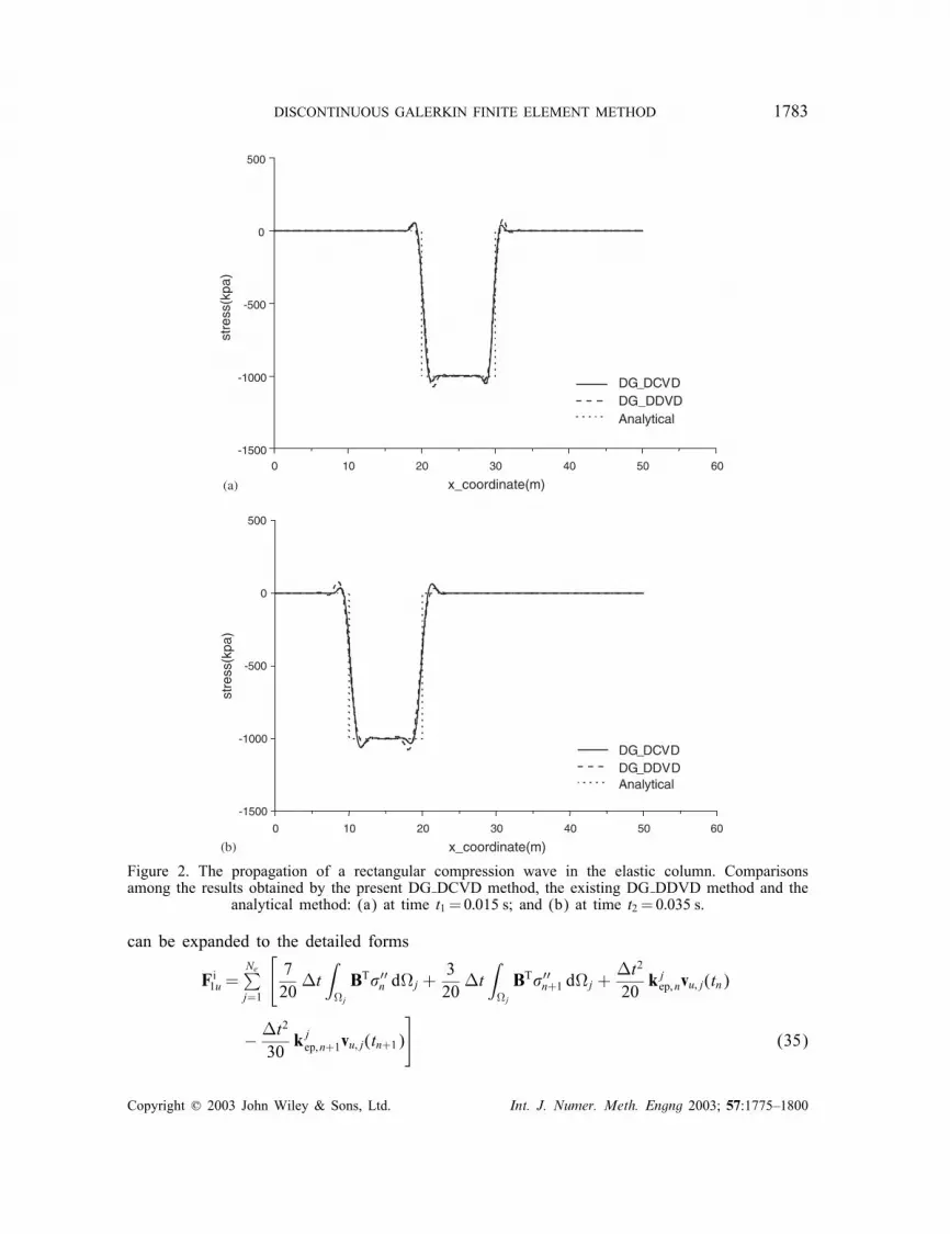
Figure 2. The propagation of a rectangular compression wave in the elastic column. Comparisonsamong the results obtained by the present DG DCVD method, the existing DG DDVD method and the

analytical method: (a) at time t1 = 0:015 s; and (b) at time t2 = 0:035 s.

can be expanded to the detailed forms

F i1u =Ne∑j=1

[720�t

∫�j

BT�′′n d�j +

320�t

∫�j

BT�′′n+1 d�j +

�t2

20kjep; nvu; j(tn)

− �t2

30kjep; n+1vu; j(tn+1)

](35)



F i2u =Ne∑j=1

[320�t

∫�j

BT�′′n d�j +

720�t

∫�j

BT�′′n+1 d�j +

�t2

30kjep; nvu; j(tn)

− �t2

20kjep; n+1vu; j(tn+1)

](36)

where kjep; n, k

jep; n+1 are the consistent tangent elastoplastic sti�ness matrices of the jth el-

ement at tn; tn+1, which are computed by the Gauss–Legendre quadrature process as soonas the consistent tangent elastoplastic modulus matrix [11] at each integration point of theelement is determined. Substituting Equations (9), (13), (25), (30) and (31) into Equa-tion (28), we obtain the following equation system from independent variations of�dn; �dn+1; �vn; �vn+1

K[12(dn + dn+1)− �t

4(vn + vn+1)− d−n

]= 0 (37a)

K[12(−dn + dn+1)− �t

4(vn + vn+1)

]= 0 (37b)

12M(vn + vn+1) + Fi1 − Fe1 +K

[�t10(−dn + dn+1)− �t2

20(vn + vn+1)

]−Mv−n = 0 (37c)

12M(−vn + vn+1) + Fi2 − Fe2 +K

[�t10(dn − dn+1) + �t2

20(vn + vn+1)

]= 0 (37d)

It is noted that the subscript of the matrix K in Equation (37) is omitted to express the equa-tion clearly, i.e. K=K(tn)=Kn. The DG �nite element formulations for the elasto-plasticdynamics can be given by using Equation (37) as follows:

dn = d−n (38a)

dn+1 = d−n +12 �t(vn + vn+1) (38b)

Mvn +�t6C(vn − vn+1) +KQ

[�t5(dn − dn+1) + �t2

60(vn + vn+1)

]+

{F i1u − F i2u

0

}

− (Fe1 − Fe2)−Mv−n = 0 (38c)

Mvn+1 +�t2C(vn + vn+1) +KQ

[�t2(dn + dn+1) +

�t2

12(vn − vn+1)

]+

{F i1u + F

i2u

0

}

−(Fe1 + Fe2)−Mv−n = 0 (38d)



0 10 20 30 40 50 60

-1500

-1000

-500

0

500

stre

ss(k

pa)

x_coordinate(m)

CG_Newmark Analytical

0 10 20 30 40 50 60

-1500

-1000

-500

0

500

stre

ss(k

pa)

x_coordinate(m)

CG_Newmark Analytical

(a)

(b)

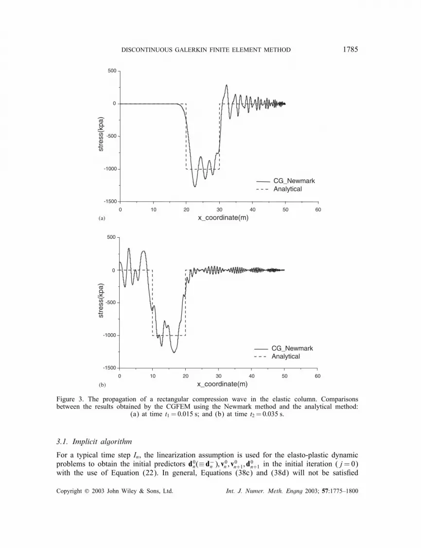
Figure 3. The propagation of a rectangular compression wave in the elastic column. Comparisonsbetween the results obtained by the CGFEM using the Newmark method and the analytical method:

(a) at time t1 = 0:015 s; and (b) at time t2 = 0:035 s.

3.1. Implicit algorithm

For a typical time step In, the linearization assumption is used for the elasto-plastic dynamicproblems to obtain the initial predictors d0n(≡ d−n ); v0n ; v0n+1; d0n+1 in the initial iteration ( j=0)with the use of Equation (22). In general, Equations (38c) and (38d) will not be satis�ed



within a tolerable error with the initial predictors. The residual vectors Rj1 and R

j2 for Equations

(38c) and (38d) in the jth iteration can be expressed as

Rj1 =Mv

jn +

�t6C(v j

n − v jn+1) +KQ

[�t5(dn − dj

n+1) +�t2

60(v j

n + vjn+1)

]+

{F i; j1u − F i; j

2u

0

}

− (Fe1 − Fe2)−Mv−n (�= 0) (39)

Rj2 =Mv

jn+1 +

�t2C(v j

n + vjn+1) +KQ

[�t2(dn + d

jn+1) +

�t2

12(v j

n − v jn+1)

]+

{F i; j1u + F

i; j2u

0

}

− (Fe1 + Fe2)−Mv−n (�= 0) (40)

With the use of the Newton–Raphson process, it is given thatM+

�t6C− �t2

12Kt

Q −�t6C− �t2

12Kt

Q

�t2C+

�t2

3Kt

Q M+�t2C+

�t2

6Kt

Q

{�v j

n

�v jn+1

}=

{−Rj1

−Rj2

}(41)

where

KtQ=

[K∗11 +K

tep K12

KT12 K22

]; Kt

ep =Ne∑l=1klep (42)

KtQ is the global tangent sti�ness matrix at the current time step, k

lep is the tangent elasto-

plastic sti�ness matrix of the lth element.An iterative computation algorithm for a typical time step In can be given as follows:

(1) dn= d−n .(2) j=0, compute predictors v0n ; v0n+1; d

0n+1 by using Equation (22).

(3) Loop for jth iteration:

(a) Computations for elastoplastic constitutive relations and nodal internal forces.Loop for each integration point in each spatial �nite element Compute �′′(dj

n+1)according to the elastoplastic constitutive model and the nodal internal force vectorf i; ju; n+1 =

∫� B

T�′′(djn+1) d�.

Compute F i; j1 ;F i; j2 by using Equations (32)–(36).Endloop

(b) Compute the residual vectors Rj1;R

j2 according to formulae (39), (40).

(c) Check for convergence of the jth iterationif ‖Rj

1‖6RTOL and ‖Rj2‖6RTOL, terminate the iteration loop.

(d) Proceed the next iteration in the loop and calculate �v jn ;�v

jn+1 by using Equa-

tion (41).



0 10 20 30 40 50 60-1500

-1000

-500

0

500

stre

ss(k

pa)

x_coordinate(m)

t=0.015s,DG_DCVD t=0.024s,DG_DCVD

0 10 20 30 40 50 60-1500

-1000

-500

0

500

stre

ss(k

pa)

x_coordinate(m)

t=0.015s,CG_Newmark t=0.024s,CG_Newmark

(a)

(b)

Figure 4. The propagation of the compression wave in the elasto-plastic column: (a) the numerical resultsby the DG DCVD method using �t=2× 10−4 s; and (b) the numerical results by the CGFEM with

the Newmark method using �t=1× 10−4 s.

(e) Update the predictors and compute the jth correctors, j⇐ j + 1

v jn = v

j−1n +�v j

n ; v jn+1 = v

j−1n+1 +�v

jn+1; dj

n+1 = d−n +

12 �t(v j

n + vjn+1) (43)

go to (a).



0 10 20 30 40 50

-4000

-3000

-2000

-1000

0

1000

2000

stre

ss, p

ress

ure(

kpa)

x coordinate(m)

DG_DCVD, stress DG_DCVD, pressure DG_DDVD, stress DG_DDVD, pressure Analytical, stress Analytical, pressure

0 10 20 30 40 50 60

-4000

-3000

-2000

-1000

0

1000

2000

stre

ss, p

ress

ure(

kpa)

x coordinate(m)

CG_Newmark, stress CG_Newmark, pressure Analytical, stress Analytical, pressure

60

(a)

(b)

0 10 20 30 40 50 60

-4000

-3000

-2000

-1000

0

1000

2000

stre

ss, p

ress

ure(

kpa)

x coordinate(m)

DG_DCVD, stress DG_DCVD, pressure DG_DDVD, stress DG_DDVD, pressure Analytical, stress Analytical, pressure

0 10 20 30 40 50 60

-4000

-3000

-2000

-1000

0

1000

2000

stre

ss, p

ress

ure(

kpa)

x coordinate(m)

CG_Newmark, stress CG_Newmark, pressure Analytical, stress Analytical, pressure

(c)

(d)

Figure 5. The propagation of rectangular compression waves in the saturated poro-elastic column inundrained conditions. Comparisons of the e�ective stress and the pore pressure wave shapes amongthe present DG DCVD method, the existing DG DDVD method, the CGFEM using the Newmarkmethod and the analytical method (AM): (a) comparisons among DG DCVD, DG DDVD and AM att=0:06s; (b) comparisons between CGFEM and AM at t=0:06s; (c) comparisons among DG DCVD,DG DDVD and AM at t=0:14 s; and (d) comparisons between CGFEM and AM at t=0:14 s.

It is worth noticing that in contrast with the existing DG �nite element formulations, in whichdn �= d−n , the characteristic dn ≡ d−n of the present DG �nite element formulation enables tosave half of the computational cost in the most time-consuming computation sub-step (a)as f iu; n=

∫� B

T�′′(d−n ) d� has been determined in the last time step. This is the prominentadvantage of the proposed version of DGFEM over the existing DG formulations.

3.2. Explicit algorithm

An explicit solution algorithm can be derived from Equations (38c), (38d), (20), (32)–(34)and given by

Mvn =Mv−n − �t

6C(vn − vn+1)−KQ

[�t5(dn − dn+1) + �t2

60(vn + vn+1)

]

−{F i1u − F i2u

0

}+�t6(f en − f en+1) (44)



0 10 20 30 40 50 60-4000

-3000

-2000

-1000

0

1000

2000

stre

ss, p

ress

ure(

kpa)

x coordinate(m)

DG_DCVD, stress DG_DCVD, pressure DG_DDVD, stress DG_DDVD, pressure

0 10 20 30 40 50 60-4000

-3000

-2000

-1000

0

1000

2000

stre

ss, p

ress

ure(

kpa)

x coordinate(m)

CG_Newmark, stress CG_Newmark, pressure

0 10 20 30 40 50 60

-4000

-3000

-2000

-1000

0

1000

2000

stre

ss, p

ress

ure(

kpa)

x coordinate(m)

DG_DCVD, stress DG_DCVD, pressure DG_DDVD, stress DG_DDVD, pressure

0 10 20 30 40 50 60

-4000

-3000

-2000

-1000

0

1000

2000

stre

ss, p

ress

ure(

kpa)

x coordinate(m)

CG_Newmark, stress CG_Newmark, pressure

(a)

(b)

(c)

(d)

Figure 6. The propagation of compression waves in the saturated poro-elasto-plastic column in drainedcondition. Comparisons of the e�ective stress and the pore pressure wave shapes among the presentDG DCVD method, the existing DG DDVD method, the CGFEM using the Newmark method: (a)comparisons between DG DCVD and DG DDVD at t=0:06s; (b) CGFEM at t=0:06s; (c) comparisons

between DG DCVD and DG DDVD at t=0:14 s; and (d) CGFEM at t=0:14 s.

Mvn+1 =Mv−n − �t

2C(vn + vn+1)−KQ

[�t2(dn + dn+1) +

�t2

12(vn − vn+1)

]

−{F i1u + F

i2u

0

}+�t2(f en + f

en+1) (45)

dn= d−n ; dn+1 = d−n +12 �t(vn + vn+1) (46)

As an explicit solution algorithm, the mass matrix M in Equations (44), (45) is lumped. Asit is noted that F i1u;F

i2u in Equations (35), (36) depend on the unknown vectors vn, vn+1; dn+1,

the iterative process for the explicit algorithm described by Equations (44)–(46) is required.

4. NUMERICAL RESULTS

In this section four example are presented to demonstrate the performance of applicability ofthe proposed discontinuous Galerkin �nite element formulations in modelling dynamic and



0 10 20 30 40 50 60

0.00

0.01

0.02

0.03

0.04

0.05

0.06

0.07

effe

citv

e pl

astic

str

ain

x coordinate(m)

DG_DCVD DG_DDVD CG_Newmark

0 10 20 30 40 50 60

0.00

0.01

0.02

0.03

0.04

0.05

0.06

0.07

effe

ctiv

e pl

astic

str

ain

x coordinate(m)

DG_DCVD DG_DDVD CG_Newmark

0.00 0.002 0.004 0.006 0.008 0.010 0.012 0.014 0.016

0.00

0.01

0.02

0.03

0.04

0.05

0.06

0.07

0.08

effe

ctiv

e pl

astic

str

ain

time(s)

CG_Newmark DG_DCVD

(a) (b)

(c)

Figure 7. The e�ective plastic strains in the saturated poro-elasto-plastic column in drained conditions:(a) the distribution along the saturated elasto-plastic column at time t=0:06s; (b) the distribution alongthe saturated elasto-plastic column at time t=0:14 s; and (c) the variation of e�ective plastic strain

occurring at the free end of the column with respect to time.

wave propagation problems in linear=non-linear solids and saturated porous media subjectedto impulse loads. The characteristics of the problems lie in the high frequency responsedominating the problems and the propagation of discontinuities or sharp gradients of thesolution. Since there are no analytical solutions available to this type of 2D problems, we �rstconsider a one dimensional stress wave propagation problem in solids, for which the analyticalsolution in elasticity exists. The example is taken from Li and Wiberg [6] but consideringboth elastic and elastoplastic wave propagation in a column with A=1:0m2 cross-section andL=50m length. The column with one end �xed and one end loaded by an axial force impulseF is analysed as a plane strain problem depicted in Figure 1. The material properties of thecolumn are chosen with Young’s modulus E=1:0× 107 kPa, Poisson’s ratio �=0 and massdensity �=2500 kg=m3. The speed of the elastic compression wave along the column axis isgiven by c=

√E=�=2× 103 m=s. The force impulse F varies with time and is expressed by

F(t)=

{1:0× 103 kN (t ∈ [0; 0:005 s])

0 (t¿0:005 s)(47)



Figure 8. Schematic statement of the two-dimensional stress wave problem in saturated poro-elasticmedia: a square panel in the plane strain subjected to an impulse inclined compression load at top left

corner: (a) geometry, �nite element mesh and the applied load; and (b) the load history.

The column is discretized in 500 uniform 4-noded linear elements of 0:1 m size along thecolumn axis. The analytical solution of the present example is a rectangular stress wavetravelling along the column axis with compression stress �= − 1× 103 kPa and the lengthof 10 m. Since the compression wave with moving discontinuous compression stress travelsalong the column axis, the present example is a typical benchmark test to the solution schemesin solving the wave propagation problems. Figure 2 gives the resulting wave propagationsolutions at two time levels of t1 = 0:015 s, t2 = 0:035 s for the example using the presentDGFEM (DG DCVD, i.e. displacements continuous velocities discontinuous) with the timestep size �t=2× 10−4 s. It is noted that the results given in Figure 2(b) is the wave formre�ected from the �xed end of the column. The results obtained by the analytical solution andthe existing DGFEM (DG DDVD, i.e. displacements discontinuous velocities discontinuous)



Figure 9. The pore pressure distributions in the square panel of saturated poro-elastic media at t=0:025s:(a) the present DG DCVD method; and (b) the CGFEM using the Newmark method.

[7] are also given in Figure 2. It is observed that the accuracy of the results obtained by usingthe present DGFEM is almost as same as that given by the DG DDVD. As compared withthe analytical solution, similar extent of the Gibbs phenomenon appears in the results givenby both the present DG DCVD and the existing DG DDVD. Figure 3 illustrates the resultsfor the same example at the same two time levels given by the CGFEM (i.e. the traditionalsemi-discrete �nite element solutions using the Newmark algorithm) using the same time stepsize. It is obvious that serious numerical oscillations appear in the results shown in Figure 3,which are clearly unacceptable. Through comparisons of the results obtained by the presentDGFEM and the CGFEM to the analytical solution the good performance of the presentDGFEM over the CGFEM in the simulation of wave propagation is obviously demonstrated.Figure 4 illustrates the numerical results in the simulation of elastoplastic compression wave

traveling along the column for the same example. The plastic yield behaviour of the materialis assumed to obey the von-Mises criterion. The evolution of the yield stress is assumedto follow the linear strain hardening rule, i.e. the current yield stress �y =�y0 + hp �� p, inwhich �y0; hp; �� p are the initial yield stress, the strain hardening parameter and the equivalentplastic strain, respectively. In the present example �y0 = 900 kPa, hp = 1155 kPa are used



Figure 10. The sphere stress distributions in the square panel of saturated poro-elastic media att=0:025 s: (a) the present DG DCVD method; and (b) the CGFEM using the Newmark method.

as material parameters. The resulting compression waves given by the proposed DG DCVDmethod using the time step size �t=2× 10−4s are illustrated in Figure 4(a), while Figure 4(b)gives the results given by the CG Newmark method using �t=1× 10−4 s. The numericalresults also illustrate much better performance of the proposed DG DCVD method than thatof traditional CG Newmak method in �ltering out the e�ects of spurious high modes andcontrolling spurious numerical oscillation in the elasto-plastic case.As the second example we consider a column of saturated porous medium with the same

geometry and �nite element mesh used for the solid column in the �rst example. At the �xedend of the column ux=Ux= uy=Uy=0 is speci�ed, which implies the undrained boundarycondition enforced. The column loaded at its free end by the axial force impulse F with theforce history given in Equation (48) is analysed as the plane strain problem

F(t)=

{4:0× 103 kN (t ∈ [0; 0:04 s])

0 (t¿0:04 s)(48)

The material property data E=1:0× 105 kPa, �s = 2500 kg=m3, Ks = 1:385× 105 kPa, �=0:3for the solid phase and kw=1× 10−6 m=s, �f = 1000 kg=m

3, Kf = 2:0× 104 kPa for the �uid



Figure 11. The shear stress distributions in the square panel of saturated poro-elastic media at t=0:025s:(a) the present DG DCVD method; and (b) the CGFEM using the Newmark method.

phase are used. The porosity is n=0:2. As the elasto-plastic response of the saturated columnis considered plastic yield behaviour of the material is assumed to obey the Drucker–Pragercriterion. The linear strain hardening rule c= c0 + hcp ��

p for the cohesion is used to govern theevolution of the elasto-plastic behaviour. Here c0; hcp; ��

p are initial cohesion, strain hardeningparameter and the equivalent plastic strain [12] de�ned for pressure dependent elasto-plasticmaterials, respectively. In the present example c0 = 10 kPa, hcp = 1 kPa, the internal frictionalangle =15◦ and the plastic potential angle =5◦ are used to account for the non-associatedplasticity. First we consider the elastic case. The speed of the compression wave is given byc=

√(�+ 2G +Q)=�∼=3:0× 102 m=s, in which � is Lame parameter and G is the shear

modulus, � is de�ned as the density of the solid–�uid mixture, namely �= n�f + (1 − n)�s.The displacements for both the solid and the �uid phases in the y-axis for all nodes areassumed �xed, i.e. uy =Uy = 0, which implies that there are neither lateral deformation norlateral drainage for the column. To consider the undrained condition, the displacements forboth the solid and the �uid phases in the x-axis are assumed bound for all nodes, i.e. ux=Ux.The analytical solutions of the present elastic case are two rectangular waves travelling alongthe column axis with the length of 12 m and the amplitudes of �′′

x =− 2719:48 kPa for the



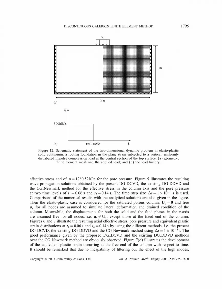
Figure 12. Schematic statement of the two-dimensional dynamic problem in elasto-plasticsolid continuum: a footing foundation in the plane strain subjected to a vertical, uniformlydistributed impulse compression load at the central section of the top surface: (a) geometry,

�nite element mesh and the applied load; and (b) the load history.

e�ective stress and of p=1280:52 kPa for the pore pressure. Figure 5 illustrates the resultingwave propagation solutions obtained by the present DG DCVD, the existing DG DDVD andthe CG Newmark method for the e�ective stress in the column axis and the pore pressureat two time levels of t1 = 0:06 s and t2 = 0:14 s. The time step size �t=1× 10−3 s is used.Comparisons of the numerical results with the analytical solutions are also given in the �gure.Then the elasto-plastic case is considered for the saturated porous column. Uy = 0 and freeuy for all nodes are assumed to simulate lateral deformation and drained condition of thecolumn. Meanwhile, the displacements for both the solid and the �uid phases in the x-axisare assumed free for all nodes, i.e. ux �=Ux, except those at the �xed end of the column.Figures 6 and 7 illustrate the resulting axial e�ective stress, pore pressure and equivalent plasticstrain distributions at t1 = 0:06 s and t2 = 0:14 s by using the di�erent methods, i.e. the presentDG DCVD, the existing DG DDVD and the CG Newmark method using �t=1× 10−3 s. Thegood performance given by the proposed DG DCVD and the existing DG DDVD methodsover the CG Newmark method are obviously observed. Figure 7(c) illustrates the developmentof the equivalent plastic strain occurring at the free end of the column with respect to time.It should be remarked that due to incapability of �ltering out the e�ect of the high modes,



Figure 13. The sphere stress distributions in the footing foundation at t=0:03 s: (a) the presentDG DCVD method; and (b) the CGFEM using the Newmark method.

the spurious numerical oscillation occurring at the free end after the wave tail passes in thenumerical solution by the CG Newmark method results in a spurious further development ofequivalent plastic strain. Hence, the extent of plastic yielding predicted by the CG Newmarkmethod is wrongly much over estimated.The objectives of the third and the forth examples are to show the applicability of the

proposed DGFEM to the elastic and the elasto-plastic wave propagation problems in solidsand saturated porous media in 2D case. As the third example, we consider the elastic wavepropagation in two-dimensional saturated porous medium. A square domain is subjected toan impulse inclined compression load at top left corner A depicted in Figure 8(a). Theexample is analysed as a plane strain problem. Geometry, boundary conditions and the�nite element mesh with 50× 50 elements are also given in the �gure. The loading



Figure 14. The e�ective stress distributions in the footing foundation at t=0:03 s: (a) the presentDG DCVD method; and (b) the CGFEM using the Newmark method.

history of the impulse load P is illustrated in Figure 8(b). The material is assumed elas-tic with E=1:0× 105 kPa, �s = 2000 kg=m3, �=0:3, Ks = 6:146× 105 kPa for the solid phaseand �f = 1000 kg=m

3, kw=1× 10−6 m=s, Kf = 2:0× 104 kPa for the �uid phase are used.The porosity is n=0:322. Figures 9–11 illustrate numerical results for the pore �uid pres-sure, the mean stress and the shear stress distributions within the domain at time t=0:025 sobtained by the proposed DG DCVD method and the CG Newmark method using the timestep �t=1× 10−3 s. It is noted that the displacements of both the solid and the �uid phasesat the left and the top boundaries of the square domain are free. Along with the P-wavepropagation within the domain, there are the S-wave propagation within the domain andRayleigh wave travelling along the free boundaries. The intersections of the P-wave with the



Figure 15. The equivalent plastic strain distributions in the footing foundation at t=0:03 s: (a) thepresent DG DCVD method; and (b) the CGFEM using the Newmark method.

free boundaries form propagating point disturbances with the P-wave speed, which generatethe Head wave on the S-wave front travelling behind the P-wave propagation. The interac-tions among P-wave, S-wave and Rayleigh wave propagation make the wave form within thedomain rather complicated. Nevertheless, the silent nature at the neighbourhood of point A,where the impulse load is applied, in the present example should be recovered with travellingwaves going ahead due to the characteristic of impulse load. Figures 9–11 demonstrate thegood performance of the proposed DG DCVD method in reproducing the silent nature at thezone near the place, where the impulse load is applied, as the resulting travelling waves goahead, while the CG Newmark method fails to do so.The fourth example concerns a footing foundation, which is 10 m deep, 20 m wide and

of in�nite length in the horizontal direction, subjected to a vertical impulse load as depictedin Figure 12. An uniformly distributed pressure load is applied to the central 2:8 m section



with the loading history shown in the �gure. The example is modeled as a transient planestrain problem of elasto-plastic solid continuum. The mesh with 50× 50 elements along withboundary conditions is illustrated in the �gure in which, by symmetry, only one half and10 m wide is taken and discretized. The material property data used are E=1:0× 105 kPa,�s = 2000 kg=m

3, �=0:3. The Drucker–Prager criterion is used to describe the elasto-plasticresponse in the problem. In the present example, c0 = 10kPa, hcp = 10kPa, =25

◦ and =5◦

are assumed. Figures 13–15 illustrate resulting spherical stress, e�ective (equivalent to sec-ond deviatoric stress invariant) stress and equivalent plastic strain distributions at t=0:03 sby using the present DG DCVD and the CG Newmark method with �t=5× 10−4 s. AgainFigure 15 demonstrates the over-estimation of equivalent plastic strains obtained by using theCG Newmark method as compared with that given by the present DG DCVD method dueto the e�ect of spurious numerical oscillation occurring in the solutions resulted from theCG Newmark method.

5. CONCLUSIONS AND DISCUSSIONS

(1) The traditional Galerkin �nite element method characterized by the semi-discrete pro-cedure in spatial domain combined with �nite di�erence methods such as the Newmarkmethod in time domain fails to capture discontinuities or sharp gradients of the solutionfor the dynamic problems subjected to impulse loads. In addition, it is also incapableof �ltering out the e�ects of spurious high modes and controlling spurious numericaloscillation.

(2) The essential features of discontinuous Galerkin �nite element methods are to use �niteelement discretizations in both space and time simultaneously and to permit assumedunknown vector and its derivative with respect to time to be discontinuous at thediscrete time levels. It can e�ectively capture the discontinuities at the wave front and�lter out the e�ects of spurious high modes and control spurious numerical oscillation.

(3) As compared with the existing DG �nite element formulations, the main distinct char-acteristic of the proposed DG �nite element formulations is that the speci�c P3–P1interpolation approximation, which uses piecewise cubic and linear interpolations forboth displacements and velocities in time domain respectively. Consequently, continu-ity of the displacement vector at each discrete time instant is automatically ensured,whereas discontinuity of the velocity vector at the discrete time levels still remains.The computational cost is then obviously saved, particularly in the materially non-linearproblems.

(4) One of the contributions of the present paper is to extend DGFEM to dynamic andwave propagation problems subjected to impulse loads in saturated poro-elastic andporo-elasto-plastic media.

ACKNOWLEDGEMENTS

The authors are pleased to acknowledge the support of this work by the National Science Foundationof China through contract=grant numbers 19832010, 50278012, 10272027 and the National Key BasicResearch and Development Program (973 Program) through contract grant number: 2002CB412709.



REFERENCES

1. Hughes TJR, Hulbert GM. Space-time �nite element methods for elastodynamics: formulations and errorestimates. Computer Methods in Applied Mechanics and Engineering 1988; 66:339–363.

2. Hulbert GM, Hughes TJR. Space-time �nite element methods for second-order hyperbolic equations. ComputerMethods in Applied Mechanics and Engineering 1990; 84:327–348.

3. Hulbert GM. Time �nite element methods for structural dynamics. International Journal for Numerical Methodsin Engineering 1992; 33:307–331.

4. Johnson C. Discontinuous Galerkin �nite element methods for second order hyperbolic problems. ComputerMethods in Applied Mechanics and Engineering 1993; 107:117–129.

5. Li XD, Wiberg NE. Structural dynamic analysis by a time-discontinuous Galerkin �nite element method.International Journal for Numerical Methods in Engineering 1996; 39:2131–2152.

6. Li XD, Wiberg NE. Implementation and adaptivity of a space-time �nite element method for structural dynamics.Computer Methods in Applied Mechanics and Engineering 1998; 156:211–229.

7. Wiberg NE, Li XD. Adaptive �nite element procedures for linear and non-linear dynamics. International Journalfor Numerical Methods in Engineering 1999; 46:1781–1802.

8. Durate A, Carmo E, Rochinha F. Consistent discontinuous �nite elements in elastodynamics. Computer Methodsin Applied Mechanics and Engineering 2000; 190:193–223.

9. Freund J. The space-continuous–discontinuous Galerkin method. Computer Methods in Applied Mechanics andEngineering 2001; 190:3461–3473.

10. Zienkiewicz OC, Shiomi T. Dynamic behaviour of saturated porous media: the generalized Biot formulation andits numerical solution. International Journal for Numerical and Analytical Methods in Geomechanics 1984;8:71–96.

11. Cris�eld MA. Non-linear Finite Element Analysis of Solids and Structures, vol.1: Essential. Wiley: Chichester,1991.

12. Duxbury PG, Li Xikui. Development of elasto-plastic material models in a natural coordinate system. ComputerMethods in Applied Mechanics and Engineering 1996; 135:283–306.


Documents

The Discontinuous Galerkin Finite Element Method and its Application to Global Wave Propagation