The Dynamics of Conditioning and Extinction

Peter R. Killeen, Federico Sanabria, and Igor DolgovArizona State University

Pigeons responded to intermittently reinforced classical conditioning trials with erratic bouts of respond-ing to the conditioned stimulus. Responding depended on whether the prior trial contained a peck, food,or both. A linear persistence–learning model moved pigeons into and out of a response state, and aWeibull distribution for number of within-trial responses governed in-state pecking. Variations of trialand intertrial durations caused correlated changes in rate and probability of responding and in modelparameters. A novel prediction—in the protracted absence of food, response rates can plateau abovezero—was validated. The model predicted smooth acquisition functions when instantiated with theprobability of food but a more accurate jagged learning curve when instantiated with trial-to-trial recordsof reinforcement. The Skinnerian parameter was dominant only when food could be accelerated ordelayed by pecking. These experiments provide a framework for trial-by-trial accounts of conditioningand extinction that increases the information available from the data, permitting such accounts tocomment more definitively on complex contemporary models of momentum and conditioning.

Keywords: autoshaping, behavioral momentum, classical conditioning, dynamic analyses, instrumentalconditioning

Estes’s stimulus sampling theory provided the first approxima-tion to a general quantitative theory of learning; by adding ahypothetical attentional mechanism to conditioning, it carried anal-ysis one step beyond extant linear learning models into the realmof theory (Atkinson & Estes, 1962; Bower, 1994; Estes, 1950,1962; Healy, Kosslyn, & Shiffrin, 1992). Rescorla and Wagner(1972) added the important nuance that the asymptotic level ofconditioning might be partitioned among stimuli that are associ-ated with reinforcers as a function of their reliability as predictorsof reinforcement; that refinement has had tremendous and wide-spread impact (Siegel & Allan, 1996). The attempt to couch thetheory in ways that account for increasing amounts of the variancein behavior has been one of the main engines driving modernlearning theory. Models have been the agents of progress, thego-betweens that reshaped both our theoretical inferences aboutthe conditioning processes and our modes of data analysis. In thistheoretical– empirical dialogue, the Rescorla–Wagner (R-W)model has been a paragon.

Despite the elegant mathematical form of their arguments, thepredictions of recent learning models are almost always qualita-tive—a particular constellation of cues is predicted to block orenhance conditioning more than others because of their differentialassociability or their history of association, and those effects aremeasured by differences in speed of acquisition or extinction or asa response rate in test trials. Individual differences, and the brevity

of learning and extinction processes, make convergence on mean-ingful parametric values difficult: There are nothing like the basicconstants of physics and chemistry to be found in psychology. Tothis is the added difficulty of a general analytic solution of theR-W model (Danks, 2003; Yamaguchi, 2006). As Bitterman(2006) astutely noted, the residue of these difficulties leaves pre-dictions that are at best ordinal and dependent on simplifyingassumptions concerning the map from reinforcers to associationsand from associations to responses:

The only thing we have now that begins to approximate a generaltheory of conditioning was introduced more than 30 years ago byRescorla and Wagner (1972). . . . . An especially attractive feature ofthe theory is its statement in equational form, the old linear equationof Bush and Mosteller (1951) in a different and now familiar notation,which opens the door to quantitative prediction. That door, unfortu-nately, remains unentered. Without values for the several parametersof the equation, associative strength cannot be computed, whichmeans that predictions from the theory can be no more than ordinal,and even then those predictions are made on the naıve assumption ofa one-to-one relation between associative strength and performance.(p. 367)

To pass through the doorway that these pioneers have openedrequires techniques for estimating parameters in which we canhave some confidence, and to achieve that requires a database ofmore than a few score learning and testing trials. But most regnantparadigms get only a few conditioning sessions out of an organism(see, e.g., Mackintosh, 1974), whereupon the subject is no longernaive. To reduce error variance, therefore, data must be averagedover many animals. This is inefficient in terms of data utilizationand also confounds the variability of learning parameters as afunction of conditions with the variability of performance acrosssubjects (Loftus & Masson, 1994). The pooled data may not yieldparameters representative of individual animals; when functionsare nonlinear, as are most learning models, the average of param-

Peter R. Killeen, Federico Sanabria, and Igor Dolgov, Department ofPsychology, Arizona State University.

This work was supported by National Institute of Mental Health GrantR01MH066860 and some of the workers by National Science FoundationIBN 0236821.

Correspondence concerning this article should be addressed to Peter R.Killeen, Department of Psychology, Arizona State University, Box871104, Tempe, AZ 85287-1104. E-mail: killeen@asu.edu

Journal of Experimental Psychology: © 2009 American Psychological AssociationAnimal Behavior Processes2009, Vol. 35, No. 4, 447–472

0097-7403/09/$12.00 DOI: 10.1037/a0015626

447

eters of individual animals may deviate from the parameters ofpooled data (Estes, 1956; Killeen, 2001). Averaging the output oflarge-N studies is therefore an expensive and nonoptimal way tonarrow the confidence intervals on parameters (Ashby & O’Brien,2008).

Most learning is not, in any case, the learning of novel responsesto novel stimuli. It is refining, retuning, reinstating, or remember-ing sequences of action that may have had a checkered history ofassociation with reinforcement. In this article, we make a virtue ofthe necessity of working with non-naıve animals, to explore waysto compile adequate data for convergence on parameters, andprediction of data on an instance-by-instance basis. Our strategywas to use voluminous data sets to choose among learning pro-cesses that permit both Pavlovian and Skinnerian associations. Ourtactic was to develop and deploy general versions of the linearlearning equation—an error-correction equation, in modern par-lance—to characterize repeated acquisition, extinction, and reac-quisition of conditioned responding.

Perhaps the most important problem with the traditional para-digm is its ecological validity: Conditioning and extinction actingin isolation may occur at different rates than when occurring inmelange (Rescorla, 2000a, 2000b). This limits the generalizabilityof acquisition–extinction analyses to newly acquired associations.A seldom-explored alternative approach consists of setting upreinforcement contingencies that engender continual sequences ofacquisition and extinction. This would allow the estimation ofwithin-subject learning parameters on the basis of large data sets,thus increasing the efficiency of data use and disentanglingbetween-subjects variability in parameter estimates from variabil-ity in performance. Against the possibility that animals will juststop learning at some point in extended probabilistic training,Colwill and Rescorla (1988; Colwill & Triola, 2002) have shownthat if anything, associations increase throughout such training.

One of Skinner’s many innovations was to examine the effectsof mixtures of extinction and conditioning in a systematic manner.He originally studied fixed-interval schedules under the rubric“periodic reconditioning” (Skinner, 1938). But, absent computersto aggregate the masses of data his operant techniques generated,he studied the temporal patterns drawn by cumulative recorders(Skinner, 1976). Cumulative records are artful and sometimeselegant, but difficult to translate into that common currency ofscience, numbers (Killeen, 1985). With a few notable exceptions(e.g., Davison & Baum, 2000; Shull, 1991; Shull, Gaynor, &Grimes, 2001), subsequent generations of operant conditionerstended to aggregate data and report summary statistics, eventhough computers had made a plethora of analyses possible. Lim-ited implementations of conditional reconditioning have begun toprovide critical insights on learning (e.g., Davison & Baum, 2006).

Recent contributions to the study of continual reconditioning arefound in Reboreda and Kacelnik (1993), Killeen (2003), and Shulland Grimes (2006). The first two studies exploited the naturaltendency of animals to approach signs of impending reinforce-ment, known as sign tracking (Hearst & Jenkins, 1974; Janssen,Farley, & Hearst, 1995). Sign tracking has been extensively stud-ied as Pavlovian conditioned behavior (Hearst, 1975; Locurto,Terrace, & Gibbon, 1981; Vogel, Castro, & Saavedra, 2006). It isfrequently elicited in birds using a positive automaintenance pro-cedure (e.g., Perkins, Beavers, Hancock, Hemmendinger, & Ricci,1975), in which the illumination of a response key is followed by

food, regardless of the bird’s behavior. Reboreda and Kacelnik andKilleen recorded pecks to the illuminated key as indicators of anacquired key–food association. In both studies, a negative contin-gency between key pecking and food, known as negative auto-maintenance (Williams & Williams, 1969), was imposed. In neg-ative automaintenance, an omission contingency is superimposedsuch that key pecks cancel forthcoming food deliveries, whereasabsent key pecks, food follows key illuminations. Key–food pair-ing elicits key pecking (conditioning), which, in turn, eliminatesthe key–food pairings, reducing key pecking (extinction), whichreestablishes key–food pairings (conditioning), and so on. Thisgenerates alternating epochs of responding and nonresponding, inwhich responding eventually moves off key or lever (Myerson,1974; Sanabria, Sitomer, & Killeen, 2006) and, to a naive recorder,“extinguishes.” Presenting food whether or not the animal re-sponds provides a more enduring, but no less stochastic, record ofconditioning (Perkins et al., 1975). The data look similar to thoseshown in Figure 1; a self-similar random walk ranging fromepochs of nonresponding to epochs of responding with high prob-abilities. Such data are paragons of what we wish to understand:How does one make scientific sense of such an unstable dynamicprocess? A simple average rate certainly will not do. Killeen(2003) showed that data like these had fractal properties, withHurst exponents in the “pink noise” range. However, other thanalerting us to control over multiple time scales, this throws no newlight on the data in terms of psychological processes.

To generate a database in which pecking is being continuallyconditioned and extinguished, we instituted probabilistic classicalconditioning, with the unconditioned stimulus (US) generally pre-sented independently of responding. Using this paradigm, weexamined the effect of duration of intertrial interval (ITI; Experi-ment 1), duration of conditioned stimulus (CS; Experiment 2), andpeck–US contingency (Experiment 3) on the dynamics of key peckconditioning and extinction.

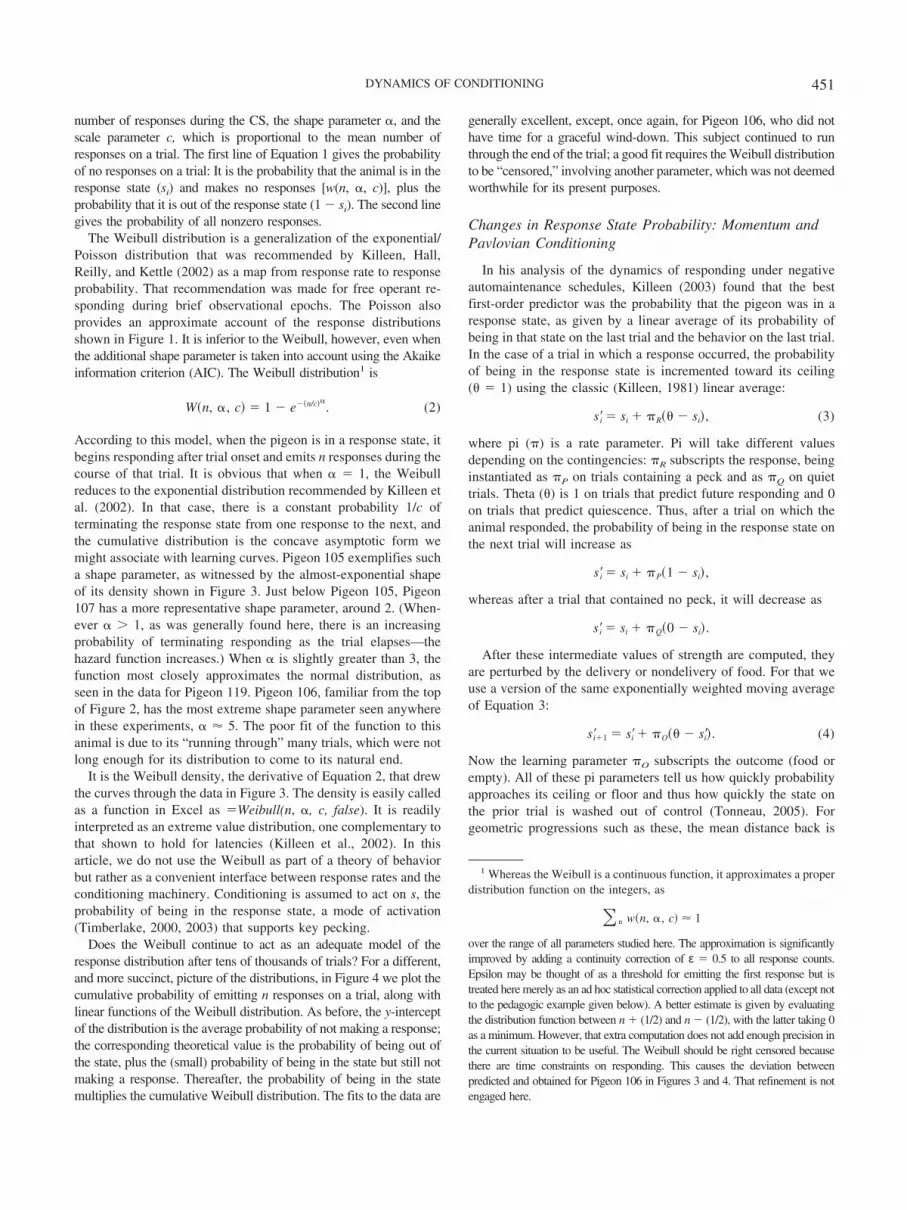
Figure 1. Moving averages of the number of responses per 5-s trial over25 trials from 1 representative subject and condition (Pigeon 98, firstcondition, 40-s intertrial interval).

448 KILLEEN, SANABRIA, AND DOLGOV

Experiment 1: Effects of ITI Duration and US Probability

Method

Subjects

Six experienced adult homing pigeons (Columba livia) werehoused in a room with a 12-hr light–dark cycle, with lights on at6:00 a.m. They had free access to water and grit in their homecages. Running weights were maintained just above their 80% adlibitum weight; a pigeon was excluded from a session if its weightexceeded its running weight by more than 7%. When required,supplementary feeding of Ace-Hi pigeon pellets (Star Milling Co.,Perris, CA) was given at the end of each day, no fewer than 12 hrbefore experimental sessions were conducted. Supplementaryfeeding amounts were based equally on current deviation and on amoving average of supplements over the past 15 sessions.

Apparatus

Experimental sessions were conducted in three MED Associates(St. Albans, VT) test chambers (305 mm long � 241 mm wide �292 mm high), enclosed in sound- and light-attenuating boxesequipped with a ventilating fan. The sidewalls and ceiling of theexperimental chambers were clear plastic. The floor consisted ofthin metal bars above a catch pan. A plastic, translucent responsekey 25 mm in diameter was located 70 mm from the ceiling,centered horizontally on the front of the chamber. The key couldbe illuminated by green, white, or red light emitted from diodesbehind the keys. A square opening 77 mm across was located 20mm above the floor on the front panel and could provide access tomilo grain when the food hopper (part H14-10R, CoulbourneInstruments, Allentown, PA) was activated. A house light wasmounted 12 mm from the ceiling on the back wall. The ventilationfan on the rear wall of the enclosing chamber provided maskingnoise of 60 dB. Experimental events were arranged and recordedvia a Med-PC interface connected to a PC computer controlled byMed-PC IV software.

Procedure

Each session started with the illumination of the house light,which remained on for the duration of the session. Sessions startedwith a 40-s ITI, followed by a 5-s trial, for a total cycle durationof 45 s. During the ITI, only the house light was lit; during the trial,the center response key was illuminated white. After completing acycle, the keylight was turned off for 2.5 s, during which foodcould be delivered. Two and a half seconds after the end of a cycle,a new cycle started, or the session ended and the house light wasturned off. Food was always provided at the end of the first trial ofevery session. Pecking the center key during a trial had no pro-grammed effect.

Initially, food was accessible for 2.5 s with reinforcement p �.1 at the end of every trial after the first, regardless of the pigeon’sbehavior. In subsequent conditions, the ITI was changed from 40 sto 20 s and then to 80 s for 3 pigeons; for the other 3 pigeons, theITI was changed to 80 s first and then to 20 s. ITIs for all pigeonswere then returned to 40 s. Each session lasted for 200 cycles whenthe ITI was 20 s, 100 cycles when the ITI was 40 s, and 50 cycleswhen the ITI was 80 s. In the last condition, the probability of

reinforcement was reduced to .05 at the 40-s ITI. One pigeon (113)had ceased responding by the end of the .1 series and was not runin the .05 condition. Table 1 arrays these conditions and thenumber of sessions at each.

Results

The first dozen trials of each condition were discarded, and theresponses in the remaining trials, averaging 2,500 per condition,are presented in the top panel of Figure 2 as mean number ofresponses per 5-s trial. The high-rate subject at the top of the graphis Pigeon 106 (cf. Figure 3 below). There appears to be a slightdecrease in average response rates as the ITI increased and a largerdecrease when the probability of food decreased from .1 to .05.Rates in the second exposure to the 40-s condition were lower thanthe first. These changes are echoed in the lower panel, which givesthe relative frequency of at least one response on a trial. Theinterposition of other ITIs between the first and second exposure tothe 40-s ITI caused a slight decrease in rate and probability ofresponding in 5 of the 6 birds, although the spread in rates in thetop panel and the error bars in the bottom indicate that that trendwould not achieve significance.

These data seem inconsistent with the many studies that haveshown faster acquisition of the key-peck response at longer ITIs. Butthese data were probabilistically maintained responses over the courseof many sessions. Only one other report, that of Perkins et al. (1975),constitutes a relatively close prequel to this one. These authors main-tained responding on schedules of noncontingent partial reinforce-ment after CSs associated with different delays, probabilities, andITIs. They used five different key colors associated with differentconditions within each study. Those that come closest to those of thepresent experiment are shown as open symbols in Figure 2. Thecircles represent the average response rate of 4 pigeons on 4-s trials(converted to this 5-s base) receiving reinforcement on one of six(�16.7%) of the trials, at ITIs of 30 s (first circle) and 120 s (secondcircle). These data also indicate a slight decrease in rates with increas-ing ITIs. Perkins et al. also reported a condition with 8-s trials and60-s ITIs involving probabilistic reinforcement. The first square inFigure 2 shows the average rate (per 5 s) of 4 pigeons at a probabilityof 3 of 27 (�11.1%); the second square, at a probability of 1 of 27(�3.7%). Their subjects, like ours (and like a few other studiesreported by these authors) showed a decrease in responding with adecrease in probability of reinforcement.

Any inferences one may wish to draw concerning these data arechastened by a glance at the intersubject variability of Figure 2 and of

Table 1Conditions of Experiment 1

Order ITI (seconds) pa Sessions

1 40 .1 20–212 20, 80 .1 21–233 80, 20 .1 20–224 40 .1 21–235 40 .05 24–29

Note. Half the subjects experienced the extreme intertrial intervals (ITIs)in the order 20 s, 80 s, and half experienced them in the other order.a p is the probability of the trial ending with food.

449DYNAMICS OF CONDITIONING

Perkins et al.’s (1975) data. The effect size is small given thatvariability, and in fact some authors such as Gibbon, Baldock,Locurto, Gold, and Terrace (1977) have reported no effect of ITI onresponse rate in sustained automaintenance conditions; others (e.g.,Terrace, Gibbon, Farrell, & Baldock, 1975) have reported someeffect. Representing intertrial variability visually is no simpler thancharacterizing intersubject variability; Figure 1 gives an approxima-tion for 1 subject (Pigeon 98) under the first 40-s ITI condition, withdata averaged in running windows of 25 trials. There is an early risein rates to around six responses per trial, then slow drift down over thefirst 1,000 trials, with rates stabilizing thereafter at around four re-sponses per trial. There may be within-session warm-up and cool-down effects not obvious in this figure. We may proceed with similardisplays and characterizations of them for each of the subjects in eachof the conditions—all different. Or we may average performance overthe whole of the experimental condition, as we did to generate thevanilla Figure 2. Or we may average data over the last 5 or 10 sessions

as is the traditional modus operandi for such data. But such averagesreduce a performance yielding thousands of bits of data to a reportconveying only a few bits of information. As is apparent from the(smoothed) trace of Figure 1, the averages do not tell the whole story.How do we pick a path between the oversimplification of Figure 2and the overwhelming complexity of figures such as Figure 1? Andhow do we tell a story of psychological processes rather than ofprocedural results? Models help, assayed next.

Analysis: The Models

Response Output Model

The goal of this research is to develop a procedure that can providea more informative characterization of the dynamics of conditioning.To do this, we begin analysis with the simplest and oldest of learningmodels, a linear learning model of associative strength. These analy-ses have been in play for more than half a century (Bower, 1994;Burke & Estes, 1956; Bush & Mosteller, 1951; Couvillon & Bitter-man, 1985; Levine & Burke, 1972), with the R-W model a modernavatar (Miller, Barnet, & Grahame, 1995; Wasserman & Miller,1997). Because associative strengths are asymptotically bounded bythe unit interval, it is seductive to think that they can be directlymapped to probabilities of responding or to probabilities of being in aconditioned state. Probabilities can be estimated by taking the numberof trials containing at least one response within some epoch, say, 25trials, and dividing that by the number of trials in that epoch (cf.Figure 1). There are three problems with this approach:

1. Twenty-five trials is an arbitrary epoch that may or maynot coincide with a meaningful theoretical–behavioralwindow.

2. Information about the contingencies that were operativewithin that epoch are lost, along with the blurring ofresponses to them.

3. Parsing trials into those with and without a responsediscards information. Response probability makes no dis-tinction between trials containing 1 response and trialscontaining 10 responses, even though they may conveydifferent information about response strength.

4. As Bitterman (2006) noted, associative strengths are notnecessarily isomorphic with probability (Rescorla, 2001).

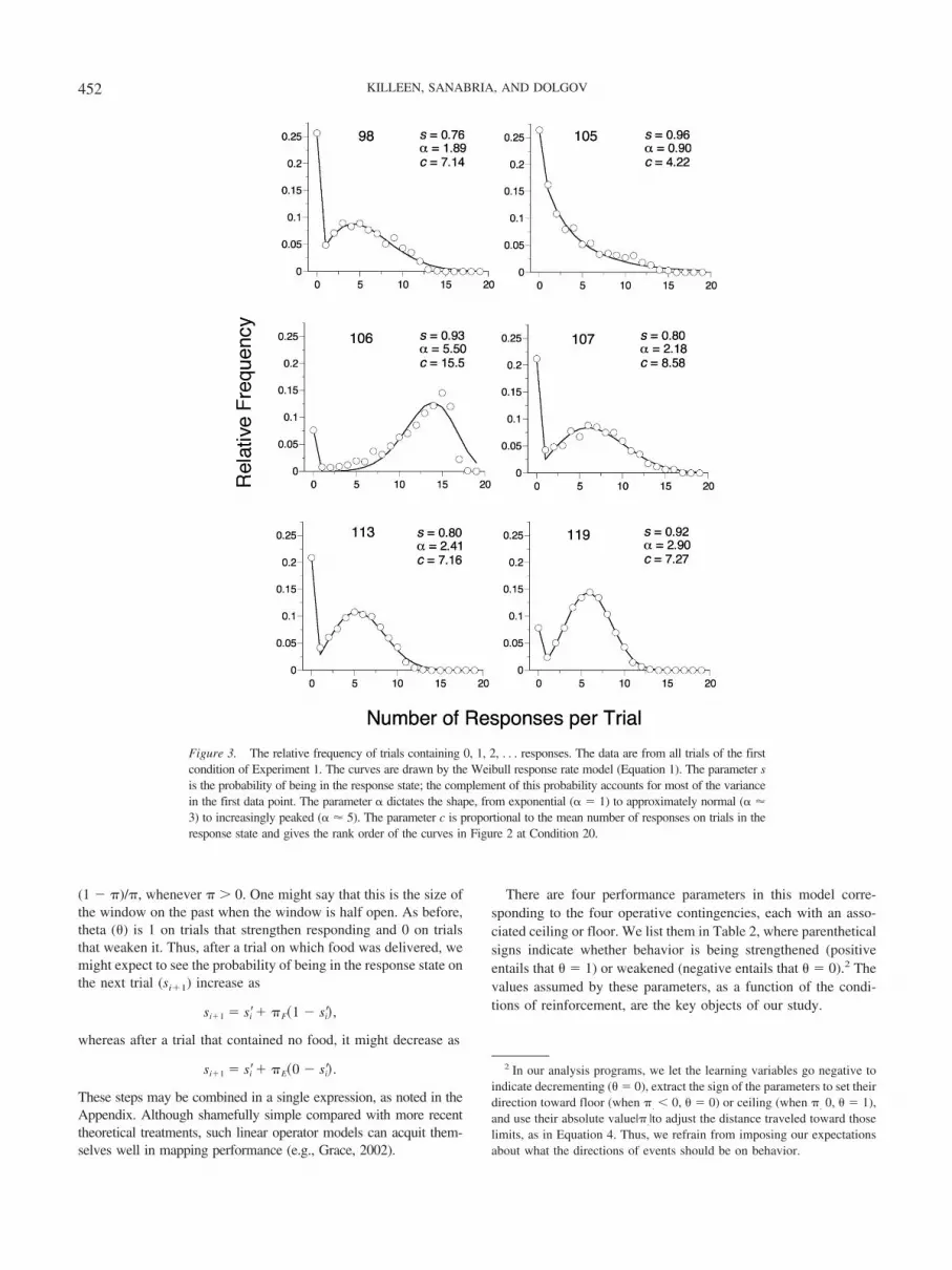
The map between response rates and inferred strength must be thefirst problem attacked. The place to start is by looking at, and char-acterizing, the distribution of responses during a CS. Figure 3 displaysthe relative frequency of 0, 1, 2, . . ., 20 responses during a trial in thefirst condition of Experiment 1 for each of its participants.

The curves through the distributions are linear functions ofWeibull densities:

p�n � 0� � si � w�n, �, c� � 1 � si,

p�n � 0� � si � w�n, �, c�. (1)

The variable si is the probability that the pigeon is in the responsestate on the ith trial. For the data in Figure 3, this is averaged over alltrials. The w function is the Weibull density with index n for the actual

Figure 2. Data from Experiment 1. Top: average number of responses pertrial (dots) for each subject, ranging from Pigeon 106 (top curve) to Pigeon105 (bottom in Condition 20). Open symbols represent data from Perkinset al. (1975). Bottom: Average probability of making at least one responseon a trial averaged over pigeons; bars give standard errors. Unbroken linesin both panels are from the Momentum/Pavlovian model, described later inthe text.

450 KILLEEN, SANABRIA, AND DOLGOV

number of responses during the CS, the shape parameter �, and thescale parameter c, which is proportional to the mean number ofresponses on a trial. The first line of Equation 1 gives the probabilityof no responses on a trial: It is the probability that the animal is in theresponse state (si) and makes no responses [w(n, �, c)], plus theprobability that it is out of the response state (1 � si). The second linegives the probability of all nonzero responses.

The Weibull distribution is a generalization of the exponential/Poisson distribution that was recommended by Killeen, Hall,Reilly, and Kettle (2002) as a map from response rate to responseprobability. That recommendation was made for free operant re-sponding during brief observational epochs. The Poisson alsoprovides an approximate account of the response distributionsshown in Figure 1. It is inferior to the Weibull, however, even whenthe additional shape parameter is taken into account using the Akaikeinformation criterion (AIC). The Weibull distribution1 is

W�n, �, c� � 1 � e��n/c��. (2)

According to this model, when the pigeon is in a response state, itbegins responding after trial onset and emits n responses during thecourse of that trial. It is obvious that when � � 1, the Weibullreduces to the exponential distribution recommended by Killeen etal. (2002). In that case, there is a constant probability 1/c ofterminating the response state from one response to the next, andthe cumulative distribution is the concave asymptotic form wemight associate with learning curves. Pigeon 105 exemplifies sucha shape parameter, as witnessed by the almost-exponential shapeof its density shown in Figure 3. Just below Pigeon 105, Pigeon107 has a more representative shape parameter, around 2. (When-ever � � 1, as was generally found here, there is an increasingprobability of terminating responding as the trial elapses—thehazard function increases.) When � is slightly greater than 3, thefunction most closely approximates the normal distribution, asseen in the data for Pigeon 119. Pigeon 106, familiar from the topof Figure 2, has the most extreme shape parameter seen anywherein these experiments, � 5. The poor fit of the function to thisanimal is due to its “running through” many trials, which were notlong enough for its distribution to come to its natural end.

It is the Weibull density, the derivative of Equation 2, that drewthe curves through the data in Figure 3. The density is easily calledas a function in Excel as �Weibull(n, �, c, false). It is readilyinterpreted as an extreme value distribution, one complementary tothat shown to hold for latencies (Killeen et al., 2002). In thisarticle, we do not use the Weibull as part of a theory of behaviorbut rather as a convenient interface between response rates and theconditioning machinery. Conditioning is assumed to act on s, theprobability of being in the response state, a mode of activation(Timberlake, 2000, 2003) that supports key pecking.

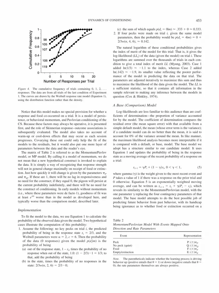
Does the Weibull continue to act as an adequate model of theresponse distribution after tens of thousands of trials? For a different,and more succinct, picture of the distributions, in Figure 4 we plot thecumulative probability of emitting n responses on a trial, along withlinear functions of the Weibull distribution. As before, the y-interceptof the distribution is the average probability of not making a response;the corresponding theoretical value is the probability of being out ofthe state, plus the (small) probability of being in the state but still notmaking a response. Thereafter, the probability of being in the statemultiplies the cumulative Weibull distribution. The fits to the data are

generally excellent, except, once again, for Pigeon 106, who did nothave time for a graceful wind-down. This subject continued to runthrough the end of the trial; a good fit requires the Weibull distributionto be “censored,” involving another parameter, which was not deemedworthwhile for its present purposes.

Changes in Response State Probability: Momentum andPavlovian Conditioning

In his analysis of the dynamics of responding under negativeautomaintenance schedules, Killeen (2003) found that the bestfirst-order predictor was the probability that the pigeon was in aresponse state, as given by a linear average of its probability ofbeing in that state on the last trial and the behavior on the last trial.In the case of a trial in which a response occurred, the probabilityof being in the response state is incremented toward its ceiling( � 1) using the classic (Killeen, 1981) linear average:

s�i � si � �R� � si�, (3)

where pi (�) is a rate parameter. Pi will take different valuesdepending on the contingencies: �R subscripts the response, beinginstantiated as �P on trials containing a peck and as �Q on quiettrials. Theta () is 1 on trials that predict future responding and 0on trials that predict quiescence. Thus, after a trial on which theanimal responded, the probability of being in the response state onthe next trial will increase as

s�i � si � �P�1 � si�,

whereas after a trial that contained no peck, it will decrease as

s�i � si � �Q�0 � si�.

After these intermediate values of strength are computed, theyare perturbed by the delivery or nondelivery of food. For that weuse a version of the same exponentially weighted moving averageof Equation 3:

s�i 1 � s�i � �O� � s�i�. (4)

Now the learning parameter �O subscripts the outcome (food orempty). All of these pi parameters tell us how quickly probabilityapproaches its ceiling or floor and thus how quickly the state onthe prior trial is washed out of control (Tonneau, 2005). Forgeometric progressions such as these, the mean distance back is

1 Whereas the Weibull is a continuous function, it approximates a properdistribution function on the integers, as

�n w�n, �, c� � 1

over the range of all parameters studied here. The approximation is significantlyimproved by adding a continuity correction of ε � 0.5 to all response counts.Epsilon may be thought of as a threshold for emitting the first response but istreated here merely as an ad hoc statistical correction applied to all data (except notto the pedagogic example given below). A better estimate is given by evaluatingthe distribution function between n (1/2) and n � (1/2), with the latter taking 0as a minimum. However, that extra computation does not add enough precision inthe current situation to be useful. The Weibull should be right censored becausethere are time constraints on responding. This causes the deviation betweenpredicted and obtained for Pigeon 106 in Figures 3 and 4. That refinement is notengaged here.

451DYNAMICS OF CONDITIONING

(1 � �)/�, whenever � � 0. One might say that this is the size ofthe window on the past when the window is half open. As before,theta () is 1 on trials that strengthen responding and 0 on trialsthat weaken it. Thus, after a trial on which food was delivered, wemight expect to see the probability of being in the response state onthe next trial (si 1) increase as

si 1 � s�i � �F�1 � s�i�,

whereas after a trial that contained no food, it might decrease as

si 1 � s�i � �E�0 � s�i�.

These steps may be combined in a single expression, as noted in theAppendix. Although shamefully simple compared with more recenttheoretical treatments, such linear operator models can acquit them-selves well in mapping performance (e.g., Grace, 2002).

There are four performance parameters in this model corre-sponding to the four operative contingencies, each with an asso-ciated ceiling or floor. We list them in Table 2, where parentheticalsigns indicate whether behavior is being strengthened (positiveentails that � 1) or weakened (negative entails that � 0).2 Thevalues assumed by these parameters, as a function of the condi-tions of reinforcement, are the key objects of our study.

2 In our analysis programs, we let the learning variables go negative toindicate decrementing ( � 0), extract the sign of the parameters to set theirdirection toward floor (when �. � 0, � 0) or ceiling (when �. 0, � 1),and use their absolute value|�.|to adjust the distance traveled toward thoselimits, as in Equation 4. Thus, we refrain from imposing our expectationsabout what the directions of events should be on behavior.

Figure 3. The relative frequency of trials containing 0, 1, 2, . . . responses. The data are from all trials of the firstcondition of Experiment 1. The curves are drawn by the Weibull response rate model (Equation 1). The parameter sis the probability of being in the response state; the complement of this probability accounts for most of the variancein the first data point. The parameter � dictates the shape, from exponential (� � 1) to approximately normal (� 3) to increasingly peaked (� 5). The parameter c is proportional to the mean number of responses on trials in theresponse state and gives the rank order of the curves in Figure 2 at Condition 20.

452 KILLEEN, SANABRIA, AND DOLGOV

Notice that this model makes no special provision for whether aresponse and food co-occurred on a trial. It is a model of persis-tence, or behavioral momentum, and Pavlovian conditioning of theCS. Because these factors may always be operative, it is presentedfirst, and the role of Skinnerian response–outcome associations issubsequently evaluated. The model also takes no account ofwarm-up or cool-down effects that may occur as each sessionprogresses. Covarying these out could only help the fit of themodels to the residuals, but it would also put one more layer ofparameters between the data and the reader’s eye.

The matrix of Table 2 is referred to as the Momentum/Pavlovmodel, or MP model. By calling it a model of momentum, we donot mean that a new hypothetical construct is invoked to explainthe data. It is simply a way of recognizing that response strengthwill not in general change maximally on receipt of food or extinc-tion. Just how quickly it will change is given by the parameters �P

and �Q. If these are 1, there will be no lag in responsiveness andno need for the construct; if they equal 0, the pigeon will persist atthe current probability indefinitely, and there will be no need forthe construct of conditioning. In early models without momentum(i.e., where these parameters were de facto 1), goodness of fit wasat least e10 worse than in the model as developed here, andtypically worse than the comparison model, described later.

Implementation

To fit the model to the data, we use Equation 1 to calculate theprobability of the observed data given the model. Two hypotheticalcases illustrate the computation of this probability:1. Assume the following: no key pecks on trial i, the predicted

probability of being in the response state si � 2/3, and theWeibull parameters were � � 2, c � 6. Then the probabilityof the data (0 responses) given the model p(di|m) is theprobability of being(a) out of the response state, 1 – si, times the probability of no

response when out of the state, 1.0: (1 � 2/3) � 1 � 1/3; tothat, add the probability of being

(b) in the state, times the probability of no responses in thestate: 2/3w(n, 2, 6) � 2/3 � 0;

(c) the sum of which equals p(di � 0|m) .333 0 0.333.2. If four pecks were made on trial i, given the same model

parameters, then the probability would be p(di � 4|m) � 0 2/3w(n, 4, 6), 0.142.

The natural logarithm of these conditional probabilities givesthe index of merit of the model for this trial: That is, it gives thelog-likelihood (LLi) of the data (given the model) on trial i. Theselogarithms are summed over the thousands of trials in each con-dition to give a total index of merit LL (Myung, 2003). Case 1added ln(1/3) �1.1 to the index, whereas Case 2 addedln(.142) �1.9, its smaller value reflecting the poorer perfor-mance of the model in predicting the data on that trial. Theparameters are adjusted iteratively to maximize this sum and thusto maximize the likelihood of the data given the model. The LL isa sufficient statistic, so that it contains all information in thesample relevant to making any inference between the models inquestion (Cox & Hinkley, 1974).

A Base (Comparison) Model

Log-likelihoods are less familiar to this audience than are coef-ficients of determination—the proportion of variance accountedfor by the model. The coefficient of determination compares theresidual error (the mean square error) with that available from asimple default model, the mean (whose error term is the variance);if a candidate model can do no better than the mean, it is said toaccount for 0% of the variance around the mean. In like manner,the maximum likelihood analysis becomes more interpretable if itis compared with a default, or base, model. The base model weadopt has a structure similar to our candidate model: It usesEquation 1 and updates the probability of being in the responsestate as a moving average of the recent probability of a response ona trial:

si 1 � �Pi � �1 � ��si, 0 � � � 1, (5)

where gamma (�) is the weight given to the most recent event andP takes a value of 1 if there was a response on the prior trial and0 otherwise. Equation 5 is an exponentially weighted movingaverage, and can be written as si 1 � si �(Pi � si), whichreveals its similarity to the Momentum/Pavlovian model, with theone parameter � replacing the four contingency parameters of thatmodel. The base model attempts to do the best possible job ofpredicting future behavior from past behavior, with its handicapbeing ignorance as to whether food or extinction occurred on a

Figure 4. The cumulative frequency of trials containing 0, 1, 2, . . .responses. The data are from all trials of the last condition of Experiment1. The curves are drawn by the Weibull response rate model (Equation 1),using the distribution function rather than the density.

Table 2Momentum/Pavlovian Model With Events Mapped OntoDirection and Rate Parameters

Event Representation

Peck P: (�)�P

No peck (quiet) Q: (�)�Q

Food F: (�)�F

Empty/extinction E: (�)�E

Note. The parentheticals indicate whether the learning process is drivingbehavior up (positive entails that � 1) or down (negative entails that �0); the rate parameters themselves are always positive.

453DYNAMICS OF CONDITIONING

trial. It is a model of perseveration, or momentum, pure andsimple. It invokes three explicit parameters: �, �, and c. Otherdetails are covered in the Appendix.

An Index of Merit for the Models

The log-likelihood does not take into account the number of freeparameters used in the model. Therefore, we use a transformationof the log-likelihood that takes model parsimony into account. TheAIC (Burnham & Anderson, 2002) corrects the log-likelihood ofthe model for the number of free parameters in the model toprovide an unbiased estimate of the information-theoretic distancebetween model and data:

AIC � 2�nP � LL�, (6)

where nP is the number of free parameters and LL is the totallog-likelihood of the data given the model. (We do not require thesecondary correction for small sample size, AICC).

We compare the models under analysis with the simple perse-veration model, the base model, characterized by Equations 1 and5. This comparison is done by subtraction of their AICs. Thesmaller the AIC, the better the adjusted fit to the data. There arenP � 3 parameters in the base model (hereinafter base), and 6parameters (8 in later versions) in the candidate model (hereinaftermodel), so the relative AIC is

Merit � Relative AIC � AIC�Base� � AIC�Model �

� 2�3 � LLB� � 2�6 � LLM�

� 2�LLM � LLB� � 6. (7)

Because logarithms of probabilities are negative, the actuallog-likelihoods are negative. However, our index of merit subtractsthe model AIC from the base AIC so that it is generally positiveand is larger because the model under purview is better than thebase model. The relative AIC is a linear function of the log-likelihood ratio of model to base (LLR � log[(likelihood ofmodel)/(likelihood of base)]). Because of the additional free pa-rameters of the model, it must account for e3 as much variance asthe base model just to break even. An index of merit of 4 for amodel means that under that model, the data are e4—approximately50 times—as probable as under the base model, after taking intoaccount the difference in number of free parameters. A net merit of4 is our criterion for claiming strong support for one model overanother. If the prior probabilities of the model under considerationand the base (or other comparison) model are deemed equal,Bayes’s theorem tells us that when the index of merit is greaterthan 4 (after handicapping for excess parameters), then the poste-rior odds of the candidate model compared with the comparison isat least 50/1.

The base model is nested in the Pavlovian/Momentum model:Setting �Q � ��P � �, and �F � �E � 0 reduces it to the basemodel. For summary data, we also display the Bayesian informa-tion criterion (BIC; Schwarz, 1978), which sets a higher standardfor the admission of free parameters in large data sets such as ours:BIC �2LL kln(n). We now apply this modeling frameworkto the results of the first experiment.

The index of merit is relative to the default base model, just asthe proportion of variance accounted for in quotidian use is relative

to a default model (the mean). If the default model is very bad, thecandidate model looks very good by comparison. If, for instance,we had used the mean response rate or probability over all sessionsin a condition as the default model, the candidate would be on theorder of e400 better in most of the experiments. A tougher testwould be to contrast the present linear operator model with themore sophisticated models in the literature, but that is not, perreviewers’ advice, included here.

Applying the Models

The AIC advantage of the Pavlovian model over the base modelaveraged 43 AIC points for the first four conditions, in which only2 of the 24 Subject � Condition comparisons did not exceed ourcriterion for strong evidence (improvement over the base model by4 points). For the last, p � .05, condition, the average meritjumped to 183 points. Figure 5 shows that the Weibull responserate parameters were little affected by the varied conditions. Theaverage value of c, 8.2, corresponded to a mean of 7.3 responsesper trial on trials on which a response was made (the mean isprimarily a function of c, but also of �). The average value of theshape parameter � was 2.4: The modal response distributionlooked like that of Pigeon 113 in Figure 3. The values of theseWeibull parameters were always essentially identical for the baseand MP models and were therefore shared by them.

The values of gamma (�), the perseveration constant in the basemodel, averaged .038 in the first four conditions and increased to.100 in the p � .05 condition. This indicates that there was agreater amount of character—more local variance—in this lastcondition for the moving average to take advantage of, a featurethat was also exploited by the MP model. There was no change inthe rate of responding—given that the pigeon is in a responsestate—as indicated by the constancy of c. All of the decrease seenin Figure 2 was the result of changes in the probability of enteringa response state, as given by the model and seen in the model’spredictions, traced by the lines in the bottom panel of Figure 2.

The weighted average parameters of the MP model are shown inthe bottom panel of Figure 5 (the values for each subject wereweighted by the variance accounted for by the model for thatsubject). Just as autoshaping is fastest with longer ITIs, the impactof the �F and �P parameters increases markedly with ITI. Theincrease in �F indicates that at long ITIs, the delivery of food,independent of pigeons’ behavior, increases the probability of aresponse on the next trial. It increases 11% of its distance toward1.0 in the 20-s ITI condition, up to 28% in the 80-s ITI condition.Also notice that �F is everywhere of greater absolute magnitudethan �E, a finding consistent with that of Rescorla (2002a, 2002b).

The increase in �P indicates that pecking acquires more behav-ioral momentum as the ITI is increased. The parameter �Q remainsaround �7% over conditions (although a drop from �5% to�10% in the first and second replication of the 40-s conditionsaccounts for the decrease in probability of responding in thesecond exposure). A trial without a response decreases the prob-ability of a response on the next by 7%. The parameter �E hoversat zero for the short and intermediate ITIs: Extinction trials add nonew information about the pigeons’ state on the next trial and donot change behavior from the status quo ante. Under these condi-tions, extinction does not discourage responding. The law ofdisuse, rather than extinction, is operative: If a pigeon does not

454 KILLEEN, SANABRIA, AND DOLGOV

respond, momentum in not responding (measured by �Q) carriesresponse probability lower and lower. At the longest ITI and in thep � .05 condition, extinction trials decrease the probability ofbeing in a response state on the next trial by 4% and 10%,respectively. When reinforcement is scarce, both food and extinc-tion matter more, as indicated by increased values of �F and �E,but the somewhat surprising effect on �E is modest compared withthe former. The importance of food when it is scarce is substan-tial—with �F increasing more than 30% in the p � .05 condition.The fall toward extinction of responding, driven by �Q and �E, isarrested only by delivery of food, a strong tonic to responding(�F), or an increasingly improbable peck, which, as reflected in�P, is associated with substantially enhanced response probabili-ties on the next trial.

We may see how close the simulations look to the real perfor-mance, such as that shown in Figure 1. We did this by replacingthe pigeon with a random number generator, using the averageparameters from the first condition, shown in Figure 5. The prob-ability of the generator’s entering a response state was adjustedusing the MP model, and when in the response state, it emittedresponses according to a Weibull distribution with the parametersshown in the top of Figure 5. Figure 6 plots the resulting data ina fashion similar to that shown in Figure 1 (a running averageof 25 trials). Comparison of the three panels cautions howdifferent a profile can result from a system operating accordingto the same fixed parameters once a random element enters.Analyses are wanted that can deal with such vagaries withoutrecourse to averaging over a dozen pigeons. By analysis on atrial-by-trial basis, the present models attempt to take a step inthat direction.

These graphs have a similar character to those generated by thepigeons (although they lack the change in levels shown by Pigeon 98in Figure 1, a change not clearly shown by most of the other subjects).The challenge is how to measure “similar” in a fashion other thanimpressionistically. Killeen (2003) showed that responding had afractal structure, and given the self-similar aspect of these curves, thatis likely to be the case here. However, the indices yielded by fractalanalysis throw little new light on the psychological processes. TheAIC values returned by the model provide another guide for thosecomfortable with likelihood analyses; they tell us how good thecandidate model is relative to a plausible contender.

The variance accounted for in the probability of responding willlook pathetic to those used to fitting averaged data: It averagesaround 10% in Experiment 1 and around 15% in the remainingexperiments. But even when the probability of a response on thenext trial is known exactly, there is probabilistic variance associatewith Bernoulli processes such as these, in particular, a variance ofp(1� p). The parameters were not selected to maximize varianceaccounted for, and in aggregates of data much of the samplingerror that is inevitable in single-trial predictions is averaged out.When the average rate over the next 10 trials, rather than the singlenext trial, is the prediction, the variance accounted for by thematrix models doubles. At the same time, the ability to speak to thetrial-by-trial adjustment of the parameters is blunted. Other anal-yses, educing predictions from the model and testing them againstthe data, follow.

Hazard Functions

That �Q and �E are negative in the p � .05 condition makes astrong prediction about sojourns away from the key: When apigeon does not respond on a trial, there is a greater likelihood thatit will not respond on the next, and yet greater on the next, and soon. Only free food (or the unlikely peck despite the odds) saves it.The probability of food is 5%, but the cumulative probability iscontinually increasing, reaching 50% after 15 trials since the firstnonresponse. The probability of returning to the key should de-crease at first, flatten, and then eventually increase. A simple testof this prediction is possible: Plot the probability of returning tothe key after various numbers of quiet trials. In making these plots,each point has to be corrected for the number of opportunities leftfor the next quiet trial. Such plots of marginal probabilities arecalled hazard functions. If there is a constant probability of return-

Figure 5. The average parameters of the base and Momentum/Pavlovianmodels for Experiment 1. The first four conditions are identified by theirintertrial interval (ITI), with the first and second exposure to the 40-s ITInoted parenthetically. The same Weibull parameters, c and �, were used forboth models. In the last condition, the probability of hopper activation ona trial was reduced from .1 to .05, with ITI � 40. The error bars delimit thestandard error of the mean. F � food; P � response; E � no food; Q � noresponse.

455DYNAMICS OF CONDITIONING

ing to the key, as would be the case if returns were at random, thehazard function would be flat. The earlier analysis predicts hazardfunctions that decrease under the pressure of the negative param-eters and eventually increase as the cumulative probability of thearrival of food increases.

Figure 7 shows the functions for individual pigeons (truncatedwhen the residual response probabilities fell to 1%). They show thepredicted form. The filled squares show the averaged results ofrunning three “statrats” in the program, with parameters takenfrom the .05 condition of Figure 5. If the model controls behaviorthe way it is claimed, the output of the statrats should resemble thatof the pigeons. There is indeed a family resemblance, although thestatrats’ hazard function was more elevated than the average of thepigeons, indicating a greater eagerness to return to the operandumthan was the case for the birds. Note also that the predicted

decrease—first 8% of the distance to 0 from �Q and then another11% from �E—predicts a decrease to 82% of the initial value afterthe first quiet—that is, from about 0.45 to 0.37 for the statrats andfrom about .28 to about .23 for the average pigeon. These are rightin line with the functions of Figure 7. The eventual flattening andslow rise in the functions is due to the cumulative effects of �F.

Is Momentum Necessary?

In the parameters �P and �Q, the MP model invokes a trait ofpersistence or momentum, which may appear supererogatory tosome readers. However, the base model, the linear average of therecent probability of responding, actually proves a strong con-tender to the MP model. It embodies the adage “The best predictorof what you will do tomorrow is what you did today.” It is thesimplest model of persistence, or momentum. We may contrast itwith a MP-minus-M model: That is, adjust the probability ofresponding on the next trial as a function of food or extinction onthe current trial, while holding the momentum parameters at zero.Even though the base model has one fewer parameter, it easilytrumps the MP-minus-M model. For example, for Pigeon 98, themedian advantage of the MP model over the base model was 14AIC points in the .1 condition and 58 points in the .05 condition.But without the momentum aspect, the MP-minus-M model tum-bles to a median of 106 points below the base model in the .1conditions and 540 points below it in the .05 condition. Howeverone characterizes the action of the �P and �Q parameters, theirpresence in the model is absolutely necessary. This analysis carriesthe within-session measurement of resistance to change reportedby Tonneau, Rıos, and Cabrera (2006) to the next level of contactwith data.

Operant Conditioning

What is the role of response–reinforcer pairing in controllingthis performance? The first analysis of these data (unreported here)consisted of a model involving all interaction terms, and thosealone: PF, PE, QF, and QE. Although this interaction model wassubstantially better than the base model (18 AIC units over all

Figure 6. Moving averages of the number of responses per 5-s trial over 25 trials from three representative“statrats,” characterized by the average parameters of real pigeons in the first condition, 40-s ITI. The onlydifference among these three panels is the random number seed for Trial 1. Compare with Figure 1.

Figure 7. The marginal probability of ending a run of quiet trials. Theunfilled symbols are for individual pigeons, and the filled circles representstheir average performance. The hazard function represented by filledsquares comes from simulations of the model.

456 KILLEEN, SANABRIA, AND DOLGOV

conditions, 73 in the p � .05 condition), it was always trumped bythe MP model (51 AIC units over all conditions, 183 in the p � .05condition).

In search of evidence of Skinnerian conditioning, we askedwhether there was a correlation between the number of responseson a trial and the probability of responding on the next trial. Anysimple correlation could be just due to persistence; however, ifresponse–reinforcer contiguity is a factor in strengthening re-sponding, then that correlation should be larger for trials that endwith food (rF) than for trials that end without food (rE). Whenmany responses occur on a reinforced trial, (a) there are moreresponses in close contiguity with the reinforcer and (b) the last ofthem is likely to be closer in time to the reinforcer than the case oftrials with only a few responses. Therefore, there should be apositive correlation between number of responses on trials endingwith food and number of responses on the next trial. It is differentfor trials that end without food: When many responses occur on anonreinforced trial, there are many more instances of the responsesubject to extinction; this should not only undermine a positivecorrelation, it could drive it negative. We can therefore test forSkinnerian conditioning by correlating the number of responses onF and E trials that had at least one response (the predictors) withthe presence or absence of a response on the next trial (thecriterion). If contiguity of multiple responses with food strengthensbehavior more than contiguity of one response to food, the corre-lation with subsequent responding should be larger when the trialwas followed by food than when it was not. That is, we wouldexpect rF � rE. We restrict the analysis to trials with at least oneresponse so that the correlation is not simply driven by the infor-mation that the pigeon is in a response state, which we know from�P has good predictive value.

We analyzed the data for all subjects from all conditions andfound no evidence for value added by multiple response–reinforcercontiguity. For no pigeon was the average correlation betweenpredictor and criterion greater when the predictor was followed byfood than when it was not. The averages over all subjects andconditions were rF � 0.035 and rE � 0.081. With an average n of150 for rF and of 1,470 for rE for each of the 29 pairs ofcorrelations, the conclusion is unavoidable: Reinforcement ontrials with multiple responses did not increase the probability of aresponse on the next trial any more than did extinction on trialswith multiple responses.

Perhaps fitting a delay-of-reinforcement model from each re-sponse to an eventual reinforcer would show evidence of operantconditioning? This was our first model of these data, not reportedhere. We found no value added by the extra parameter (the slopeof the delay-of-reinforcement gradient).

Convinced that there must be some way to adduce evidence of(adventitious) operant conditioning, we turned to the next analysis.It remains possible that reinforcement increases the probability ofstaying in the response state on the next trial: Possibly the com-mitment to a behavioral module (Timberlake, 1994), rather thanthe details of actions within the module, is what gets strengthenedby reinforcement. To test this hypothesis, we added conditioningfactors, �PF and �PE, to the model. If response–reinforcer conti-guity added strengthening–prediction beyond that afforded by theindependent actions of persistence and of food delivery, one orboth of these parameters should take values above zero and shouldadd significantly to predictive accuracy when it does. We measure

accuracy with the AIC score; any increase (after handicapping forthe added parameter) lends credibility, and increases by at least 4constitute strong evidence.

The average value of �PF across the 29 cases was 0.064: Thatis, the probability of a response on the next trial increased by 6%beyond that predicted by momentum and mere delivery of food(independent of the presence or absence of a peck). For 2 birds,107 and 119, there was no advantage, and �PF remained close tozero, as often negative as positive. Of the 19 remaining Pigeon �Condition cases, 11 showed an AIC advantage for the addedparameter, 5 of them meeting our criterion for strong evidence. Ofthe 4 birds that showed evidence of Skinnerian conditioning, theaverage value of �PF was 8%, which may be compared with 16%for �P and 14% for �F. Examining the data on a condition-by-condition basis, all 4 of these pigeons showed evidence of Skin-nerian conditioning in the 20-s ITI condition (3 of them, strongevidence), and in all cases but one �PF was larger than either �P

or �F. Across all 6 pigeons, the advantage of adding the contiguityparameter was 2.6 AIC points at the 20-s ITI 20, 0.8 at the 40-sITI, and �1.5 at the 80-s ITI. (The negative value indicates that thecost of the extra parameter in Equation 7 is not repaid by increasedpredictive ability.) In the p � .05 condition, the total advantageconferred by the �PF parameter increased to 6.4. (When theSkinnerian parameter comes into play, there is typically a read-justment of the other parameters that had been tasked with pickingup the slack.) The Skinnerian extinction parameter �PE was almostnever called into play and exerted negligible improvement in thepredictions. Parameter values for each pigeon are listed in Table 3;indices of merit, in Table 4.

These results indicate that Skinnerian conditioning was stron-gest where Pavlovian conditioning was weakest—whether thatweakness was the result of a small ITI-to-trial ratio (20-s ITI) or toa less reliable CS ( p � .05). This is consistent with the findings ofWoodruff, Conner, Gamzu, and Williams (1977). We retain �PF

and �PE in subsequent analyses, in which we call the full modelthe Momentum/Pavlovian/Skinnerian (MPS) model.

Implications for Acquisition and Extinction

On the basis of Equation 4 and the parameters shown in Fig-ure 5, we may predict the courses of acquisition and extinction insimilar contexts—it is given by Equation A5 in the Appendix. Forthe parameters in Figure 5, the MPS model predicts faster acqui-sition at longer ITIs—the trial spacing effect, along with an in-creasing dependence on the original starting strength (derived fromhopper training) as trial spacing decreases. Pretraining plays acritical role in determining the speed of acquisition (Davol, Stein-hauer, & Lee, 2002; Downing & Neuringer, 2003); the currentanalysis suggests that this is in part because of elevation of theinitial probability of a response, s0, possibly through generalizationof hopper stimuli and key stimuli (Sperling, Perkins, & Duncan,1977; Steinhauer, 1982). Conditioning of the context proceedsrapidly, however, so that more than a few pretraining trials in thesame context will slow the speed of subsequent key conditioning(Balsam & Schwartz, 2004).

The predicted number of trials to criterion show an approximatepower-law relation between trials to acquisition and the ITI (Gib-bon et al., 1977). Those researchers, along with Terrace, Gibbon,Farrell, and Baldock (1975), found that both acquisition and re-

457DYNAMICS OF CONDITIONING

sponse probability in steady-state performance after acquisitioncovaried with the ratio of trial duration to ITI. Gibbon, Farrell,Locurto, Duncan, and Terrace (1980) found the permutation thatpartial reinforcement during acquisition had no effect on trials toacquisition, when those were measured as reinforced trials toacquisition. This is consistent with the acquisition equations in theAppendix. Despite these tantalizing similarities, however, the ob-vious difference in the parameters for the p � .1 and p � .05conditions seen in Figure 5 undermines confidence in extrapola-tions to typical acquisition, where p � 1.0.

It is possible to test the predictions for extinction within thecontext of the present experiments, where parameter change is notso central an issue, for there were long stretches (especially in thep � .05 condition) without food. The relevant equation, trans-planted from the Appendix (Equation A6), is

si 1 � si�1 � �E��1 � �P�Q�1 � si��, (8)

where the strength si 1 gives the probability of entering a responsestate on that trial. All parameters are positive, with asymptotes of0 or 1 used as appropriate to the signs shown in Figure 5. Neither�F nor �PF appear because there are no food trials in a series ofextinction trials, and �PE is typically small and its work can beadequately handled by �E. The probability of responding on a trialdecreases with �E as expected (note the element ��E si)—substantially when si is large, not much at all when si is small. Onlythe difference in the two momentum parameters, �P � �Q, affectsthe prediction; for parsimony, we collapse those into a singleparameter representing their difference, �P�Q � �P � �Q. Equa-tion 8 makes an apparently counterfactual prediction.

A Surprising Prediction

Inspection of Figure 5 shows that �P�Q is generally positive.Because it multiplies the probability of not responding (Equation 8contains the element �P�Q[1 � si]), on average �P�Q increasesthe probability of responding on each trial and does so more as si

gets small. Depending on the specific value of the parameters, thisrestorative force may be sufficient to forestall extinction. To showthis more clearly, we solve Equation 8 for its fixed point, or steadystate, which occurs when si 1 � si:

s� � 1 ��E

�P�Q�1 � �E�, (9)

where 0 � �P�Q(1 � �E) � �E; this is the level at whichresponding is predicted to stabilize after a long string of extinctiontrials.

If response probability fluctuates below the level of si, the nextresponse (if and when it occurs, which it does with probability si)will drive probability up, and if it fluctuates above this level, thenext trial will drive it down. For responding to extinguish, it isnecessary that the force of extinction be greater than the restoringforce:

�E ��P�Q

1 � �P�Q. (9)

This is automatically satisfied whenever momentum in quies-cence, �Q, is greater than momentum in pecking �P—whenever�P�Q is negative. That is especially likely to be the case in rich

Table 3Parameter Values of the Base and Momentum/Pavlovian/SkinnerianModels for the Data of Experiment 1

Bird no. Parameter 20 401 402 80 .05

98 � .02 .03 .05 .02 .08c 8.78 6.93 5.31 7.77 5.90� 3.00 2.08 1.55 2.30 1.76P .00 .02 .04 �.01 .27Q �.02 �.03 �.05 �.01 �.19F .00 .05 .03 .22 .00E .00 .00 .00 .00 .01PF .20 .00 .13 .00 .00PE .00 .00 .00 .00 �.08

105 � .05 .04 .11 .10 .12c 5.69 5.12 7.18 7.49 5.74� 1.56 1.31 2.13 2.33 1.62P .04 .05 .19 .61 .32Q �.04 �.04 �.24 �.15 .02F .03 .00 .56 .33 .34E .00 .00 .03 �.10 �.30PF .14 .04 .34 .00 .00PE .00 .02 �.04 .00 .28

106 � .05 .02 .07 .02 .12c 12.71 13.88 13.29 14.35 12.40� 3.54 4.49 3.55 4.25 2.36P .05 .10 .18 .17 .30Q �.06 �.07 �.14 �.07 �.16F .00 .00 .27 .27 .54E .01 .03 .00 �.02 �.03PF .19 .43 .16 .10 .00PE .00 �.01 �.01 .00 �.01

107 � .02 .05 .05 .01 .04c 8.56 8.20 7.47 8.69 8.00� 2.57 2.20 2.11 2.22 2.00P .06 .00 .04 .00 .06Q �.03 �.04 �.06 �.01 �.05F .29 .27 .12 .30 .30E �.02 .00 .00 �.01 .00PF .00 .00 .00 .00 .00PE .00 .00 .00 .00 �.04

113 � .02 .05 .04 .03c 6.90 5.45 4.79 6.45� 2.51 2.22 1.76 2.46P .02 .06 .06 .68Q �.02 �.06 �.04 .12F .00 .14 .00 �.06E .00 �.01 .00 �.16PF .05 .00 .00 .00PE .00 .00 �.01 .00

119 � .01 .01 .03 .02 .06c 8.12 7.17 6.41 7.78 6.76� 3.17 2.92 2.49 2.30 2.44P .21 .28 .04 �.01 .48Q �.05 �.07 �.04 �.01 �.17F .90 .65 .31 .23 .50E �.02 �.03 .00 .00 .00PF �.02 .00 �.01 .00 .00PE .09 .17 .00 .00 �.04

Note. � � the rate constant for the comparison base model; c � theWeibull rate constant; � � the Weibull shape constant; the remainingletters indicate the rate constants brought into play on trials with (P) orwithout (Q) a response; with (F) or without (E) food; and the Skinnerianinteraction terms PF and PE.

458 KILLEEN, SANABRIA, AND DOLGOV

contexts where quiescence on the target key may be associatedwith foraging in another patch or responding on a concurrentschedule. For the parameters in Figure 5 under p � .05, however,this is never the case; indeed, the more general inequality ofEquation 10 is never satisfied. Therefore Equations 8 and 9 makethe egregious prediction that the probability of responding will fall(with a speed dictated by �E) to a nonzero equilibrium dictated byEquation 9. We may directly test this derivation by plotting thecourse of extinction within the context of dynamic reconditioningof these experiments. The best data come from the p � .05condition, which contained long strings of nonreinforced respond-ing. The courses of extinction, along with the locus of Equation 8,are shown in Figure 8.

Do Equations 8–10 condemn the birds to an endless Sisypheanrepetition of unreinforced responding? If not, what then savesthem? Those equations are continuous approximations of a finiteprocess. Because the right-hand side of Equation 8 is multiplied bysi, if that probability ever does get close enough to 0 through alow-probability series of quiescent trials, it may never recover. Itis also likely that after hundreds of extinction trials, the governingparameters would change, as they did across the conditions of thisexperiment, releasing the pigeons to seek more profitable employ-ment. The maximum number of consecutive trials without food inthis condition averaged around 120. Surely over unreinforcedstrings of length 95 through 120, the probability of respondingwould be decreasing toward zero. Such was the case for 2 pigeons,98 and 107, whose response probability decreased significantly(using a binomial test) to around 5% (the drift for 107 is alreadyvisible in Figure 8). The predicted fixed points and obtainedprobabilities for another 2, 105 and 119, were invariant, .203.19and .773.78, respectively; Pigeon 106 showed a decrease in

probability, .613.54, that was not significant by the binomial test.The substantial momentum shown in Figure 8, and extended insome cases by the binomial analysis, resonates with the data ofKilleen (2003; cf. Sanabria, Sitomer, & Killeen, 2006), wheresome pigeons persisted in responding over many thousands oftrials of negative automaintenance.

The validation of this unlikely prediction should, by someaccounts of how science works, lend credence to the model. But itcertainly could also be viewed as a fault of the model, in that itpredicts the flatlines of Figure 8, when few pigeons, except per-haps those subjected to learned helplessness training, will persist inunreinforced responding indefinitely. On that basis we could rejectthe MPS model because it does not specify when the pigeons willabandon a response mode (as reflected in changes in the persis-tence parameters). Conversely, the data of Figure 8 indict modelsthat do not predict the plateaus that are clearly manifest there. Onthat same basis, we could therefore reject all of the remainingmodels. But perhaps the most profitable path is to reject Popper infavor of MPS, which permits tracking of parameters over anindefinite number of trials, to see when, under extended dashing ofexpectations, those begin to change.

Equation 8 contains the element si(1 � si): The product of theprobability of a response and its complement enters the predictionof response probability on the next trial. This element is the coreof the “logistic map.” Depending on the coefficient of this term,the pattern of behavior it governs is complex and may becomechaotic. This, along with the multiple timescales associated withthe rate parameters, is the origin of the chaos that Killeen (2003)found in the signatures of pigeons responding over many trials ofautomaintenance and the factor that gives the displays in Figures 1and 6 their self-similar character.

Table 4Indices of Merit for the Model Comparison of Experiment 1

Bird no. Metrica 20 401 402 80 .05

98 CD 0.03 0.06 0.17 0.06 0.19�IC 9 �1 32 29 115BIC �17 �18 15 20 97

105 CD 0.07 0.02 0.17 0.13 0.16�IC 57 72 162 105 375BIC 38 55 134 91 352

106 CD 0.17 0.03 0.18 0.05 0.19�IC 47 40 69 5 217BIC 22 17 46 �14 193

107 CD 0.04 0.09 0.14 0.05 0.11�IC 101 40 13 18 88BIC 82 34 2 8 70

113 CD 0.04 0.07 0.30 0.03�IC 12 27 38 24BIC �7 10 19 9

119 CD 0.02 0.01 0.02 0.07 0.07�IC 57 40 8 29 87BIC 25 17 �14 19 69

Group CD 0.06 0.05 0.16 0.06 0.14�IC 47 36 54 35 176BIC 24 19 34 22 156

Note. Italics indicate averages over the group.a The metrics of goodness of fit for the models are the coefficient of determination (CD), the Akaike informationcriterion (AIC), and the Bayesian information criterion (BIC). Values of the last two greater than 4 constitutestrong evidence for the Momentum/Pavlovian/Skinnerian model.

459DYNAMICS OF CONDITIONING

Experiment 2: Trial Duration

The trial-spacing effect depends on the duration of both the ITIand the trial; arrangements that keep that ratio constant often yieldabout the same speed of acquisition of responding. Therefore, totest the generalizability of both the response rate model and theMPS model, we systematically varied trial duration in this exper-iment.

Method

Subjects and Apparatus

Six experienced adult homing pigeons, housed in similar con-ditions as in Experiment 1, served. Pigeons 105, 106, 107, 113, and119, who had participated in Experiment 1, were joined by 108,who replaced 98. The apparatus remained the same.

Procedure

Seven sessions of extinction were conducted before beginning thisexperiment. In extinction, stimulus conditions were similar to those ofExperiment 1, but the ITI was 35 s and trial duration was 10 s; no foodwas delivered ( p � 0). In experimental conditions, food was deliv-ered with p � .05, the ITI remained 35 s, and trial duration varied,starting at 10 s for 13 sessions. Then half the subjects went tothe 5-s CS condition, and half went to the 20-s CS condition.Finally, the 10-s CS was recovered. All sessions lasted 150trials; Table 5 reports the number of sessions per condition.

Results

In the last session of extinction, the typical pigeon pecked on 3% ofthe trials. This is a lower percentage than shown in Figure 8 becauseit follows six sessions of extinction. Extinction happens. On movingto the first experimental condition, this proportion increased to anaverage of 75%. The average response rates and probabilities ofresponding are shown in Figure 9. Both rates and probabilities de-creased as CS duration increased. Also shown are average rates from4 pigeons studied by Perkins et al. (1975) for CS durations of 4, 8, 16,and 32 s for pigeons maintained on probabilistic ( p � 1/6) Pavlovianconditioning schedules, with an ITI of 30 s. (The average rate at 32 swas 0.2 responses per second). The higher rates for Perkins et al.’ssubjects are probably due to their higher rates of reinforcement (1/6trials compared with our 1/20). The decrease in response rate with CSduration is consistent with the data of Gibbon et al. (1977), who found

Figure 8. The average probability of responding as a function of the number of trials since reinforcement, fromthe p � .05 condition. The number of observations decreases by 5% from one trial to the next, from hundredsfor the first points to 10 for the last displayed. The curve comes from Equation 8, using parameters �P–Q and�E fit to these data.

Table 5Conditions of Experiment 2

Order Trial duration (seconds) Sessions

1 10 132 5, 20 133 20, 5 134 10 14

Note. Half the subjects experienced the extreme trial durations in theorder 5 s, 20 s; half experienced them in the other order.

460 KILLEEN, SANABRIA, AND DOLGOV

that rate decreased as a power function of trial duration, with exponent�0.75. A power function also described rates in these experiments,accounting for 99% of the variance in the average data, with exponent�0.74.

The MPS model continued to outperform the base momentummodel, with an average advantage of 130 AIC units, giving it anadvantage in likelihood of e130. The parameters were largerthan those found in the last condition of Experiment 1 (seeFigure 10 and Tables 6 and 7) and on average did not showmajor changes among conditions, although the impact of a trialwith food was greatest in the first condition studied, 10(1), andthere were slight decreases in �PF and �Q as a function of trialduration. There was a moderate increase in the average numberof responses emitted (c, top panel of Figure 10) as trial durationincreased from 5 s to 20 s; the birds adjusted to having longerto peck before the chance of reinforcement carried them to thehopper.

Despite the importance of trial duration for acquisition ofautoshaped responding, the changes in the conditioning param-

eters as a function of that variable were modest. They did,however, work in unison to decrease response rates as the CSduration increased. The only moderate changes may be due tothe very short ITI in this series. The biggest effect was thetransition into the first condition of the experiment, the first10-s CS, after several sessions of extinction, where the Pavlov-ian and Skinnerian learning parameters �F and �PF were aslarge or larger than in any other conditions. Empty trials,although common, had little effect on behavior because �E wasgenerally very close to 0. In general, the dominance of �F over�PF (and the other parameters), especially at the longest CSduration, may have been due to the extended opportunity fornonreinforced pecking in that long CS condition.

In interpreting these parameters, and those of Figure 5, it isimportant to keep in mind that �E was in play on 95% of the trials,

Figure 10. The average parameters of the base and Momentum/Pavlovian/Skinnerian models for Experiment 2. The conditions are iden-tified by their trial duration, with the first and second exposure to the 10-sintertrial interval noted parenthetically. The same Weibull parameters, cand �, were used for both models. The error bars delimit the standard errorsof the mean. �PF is traced by a dashed line, and �PE by a dotted line. F �food; P � response; E � no food; Q � no response; PF and PE �Skinnerian interaction terms.

Figure 9. Data from Experiment 2. Top: average response rate (dots) foreach subject. Open circles gives average rate and squares represent datafrom Perkins et al. (1975). Bottom: Average probability of making at leastone response on a trial averaged over pigeons; bars give standard errors.Unbroken lines in both panels are from the Momentum/Pavlovian/Skinnerian model. CS � conditioned stimulus.

461DYNAMICS OF CONDITIONING

either �P or �Q on every trial, �F on 5% of the trials, and �PF onfewer than 5% of the trials. Thus, a trial with food in this exper-iment would move response strength a very substantial 60% of theway to maximum—but this happened only rarely.

Once again, the quiescence parameter �Q was the primary forcedriving the probability of entry into the response state toward 0,having a mean value of �.215. This value, so close to that for �P

(.222), indicates that the momenta of pecking and quiescence were,on average, essentially identical. This situation, �P�Q 0, willnot sustain asymptotic responding above zero (see Equation 10);with so short an ITI, that is perhaps not surprising. The success ofthis prediction is illustrated in Figure 11 for the 5-s CS condition,which showed no evidence of a plateau. The slight negativeacceleration is due to the dominance in the pooled data of profilesfrom pigeons whose �P�Q was negative. This analysis may throwadditional light on within-session partial reinforcement extinctioneffects (Rescorla, 1999) because different animals or paradigmsmay have quite different values of �P�Q.

Because these conditions were preceded by seven sessions ofextinction, the opportunity arises to trace the course of reacquisitionfor these birds and compare it with the model’s profiles. The proba-bility of a response on each of the first 100 trials, averaged over allpigeons and over a 7-trial moving window, is drawn as circles inFigure 12. The MPS model provides a closed-form solution to theacquisition curve. The equation is shown in the Appendix; the smoothacquisition curve is shown in Figure 12. The curve provides—atbest—an idealized picture of the process because it assumes thatresponse probability is dependent on the programmed probability offood, p, which is uniform over trials. MPS can do better than that byusing the real thing—whether food was delivered or not—to inform itspredictions. Replacing p with the trial-to-trial relative frequencyacross pigeons, represented by the hatch marks in the figure, and

keeping all parameters otherwise the same, gives the jagged curve, abetter characterization of the process. Figure 12 draws a graphicreminder of a point made by Benedict and Ayres (1972): Nonlineardynamic processes, such as the course of learning, can be extremelysensitive to the particulars of stochastic processes. Generic modelswith asymptotic parameters, such as limiting values for p or even fors, will provide at best an idealization; the dynamics is in the details.The textbook-smooth curve shown in Figure 12 does not represent thecharacter of the data. Over the full course of the experimental condi-tions, MPS easily supports its burden of parameters, as attested by itsAICs, and carries us from milquetoast descriptions to the jaggedprofiles of Figure 12—to predictions with teeth.

All of the manipulations so far have been classic Pavlovian kinds,varying experimental parameters that did not interact with behavior,and those only modestly (see, e.g., Schachtman, 2004, for somemodern developments). Although noncontingent food presentationcan leave response–outcome associations intact (Colwill, 2001; Res-corla, 1992), all of the response–outcome associations up to this pointwere adventitious. We conducted the last series of experiments tocomplement those open-loop Pavlovian operations with closed-loopinstrumental operations having more consistent contingencies.

Experiment 3: Fixed Ratio and Differential Reinforcementof Other Behavior Contingencies

Method

Subjects and Apparatus

Eight experienced adult homing pigeons, half having served inother experiments reported in this article, were used. They weremaintained under the same conditions as the prior experiments.The apparatus was the same as used before.

Table 6Indices of Merit for the Model Comparison of Experiment 2

Bird no. Metrica 5 101 102 20

105 CD 0.01 0.32 0.26 0.29�IC 5 347 365 360BIC 0 319 342 338

106 CD 0.27 0.07 0.26 0.15�IC 169 106 285 163BIC 152 79 262 141

107 CD 0.25 0.12 0.22 0.11�IC 193 141 172 119BIC 170 118 155 97

108 CD 0.10 0.14 0.08 0.05�IC 79 127 49 37BIC 62 104 32 20

113 CD 0.23 0.15 0.04 0.05�IC 183 214 40 34BIC 155 197 12 17

119 CD 0.12 0.11 0.12 0.10�IC 75 56 81 54BIC 53 45 53 32

Group CD 0.18 0.12 0.22 0.10�IC 124 134 127 87BIC 107 111 104 64

a The metrics of goodness of fit for the models are the coefficient of determination (CD), the Akaike informationcriterion (AIC), and the Bayesian information criterion (BIC). Values of the last two greater than 4 constitutestrong evidence for the Momentum/Pavlovian/Skinnerian model.

462 KILLEEN, SANABRIA, AND DOLGOV

Procedure

Before the experiment proper, six to seven sessions of extinctionwere conducted with a 35-s ITI and 10-s trial duration; the prob-ability of food delivery was zero ( p � 0). A preliminary series ofexperiments was conducted with p � .05. In these conditions,which we call fixed-ratio 3 (FR 3) and differential reinforcementof other behavior (DRO), reinforcement contingencies were in-tended to vary response–reinforcement contiguity in opposite di-rections. However, the low probability of exposure to those con-tingencies—5% of the trials at most, usually less—gave animalsinsufficient exposure to the Skinnerian contingencies: In a number

Figure 11. The average probability of responding as a function of thenumber of trials since reinforcement, from the 5-s conditioned stimulus(CS) condition of Experiment 2, pooled over subjects. The number ofobservations decrease by 5% from one trial to the next, from 485 for thefirst point to 29 for the last displayed. The curve comes from Equation 8,using parameters �P–Q and �E fit to these data.

Figure 12. The average probability of responding as a function of thenumber of trials since the start of the 10-s conditioned stimulus condition ofExperiment 2, pooled over subjects, and represented as a seven-trial movingaverage (circles). The hatch marks indicate trials on which 1 (plotted at p �1/6) or 2 (plotted at p � 2/6) pigeons happened to have received food. In nocases did the same trial end with food for more than 2 pigeons. The smoothcurve comes from the Momentum/Pavlovian/Skinnerian model, setting p �.06, with all other parameters fit to these data. The jagged curve comes fromthe same equation with the same parameters but uses the obtained relativefrequency of food as given by the hatch marks.

Table 7Parameter Values of the Base and Momentum/Pavlovian/Skinnerian Models for the Data of Experiment 2

Bird no. Parameter 5 101 102 20

105 � 0.01 0.17 0.13 0.14c 8.47 7.07 6.45 15.67� 3.03 1.53 1.58 1.73P 0.00 0.16 0.21 0.34Q �0.01 �0.27 �0.33 �0.45F 0.13 0.83 0.55 0.71E 0.00 0.02 0.01 0.04E 0.00 0.02 0.01 0.04E 0.00 0.02 0.01 0.04

106 � 0.12 0.09 0.15 0.18c 12.87 16.53 16.87 22.21� 3.32 2.00 1.78 1.30P 0.31 0.08 0.45 0.30Q �0.19 �0.21 �0.30 �0.29F 0.68 0.35 0.44 0.60E 0.00 0.10 �0.14 0.02PF 0.00 0.62 0.00 0.00PE �0.03 �0.02 �0.08 �0.03

107 � 0.14 0.14 0.15 0.11c 8.95 9.26 11.73 17.65� 2.68 1.60 1.73 1.42P 0.00 0.00 0.19 �0.04Q �0.14 �0.14 �0.16 �0.19F 0.69 0.69 0.48 0.38E �0.03 �0.02 �0.02 0.01PF 0.00 0.00 0.00 0.00PE 0.17 0.18 0.00 0.15

108 � 0.11 0.14 0.08 0.05c 5.70 119.00 41.00 29.00� 1.45 0.15 0.06 0.08P 0.10 0.29 0.02 0.00Q �0.15 �0.24 �0.03 �0.08F 0.55 1.00 0.20 0.30E 0.04 0.03 0.00 �0.01PF 0.00 0.00 0.00 0.00PE 0.00 �0.02 0.00 0.10

113 � 0.13 0.12 0.07 0.08c 17.22 10.77 10.08 11.40� 2.01 2.12 2.60 1.21P 0.39 0.54 0.12 0.06Q �0.19 �0.10 �0.11 �0.09F 0.34 0.87 0.39 0.27E �0.06 �0.10 0.02 0.02PF 0.34 0.00 0.02 0.00PE 0.00 0.00 0.00 0.00

119 � 0.08 0.05 0.08 0.06c 10.04 15.25 16.99 19.68� 2.96 3.18 3.61 2.35P 0.26 0.00 0.41 0.05Q �0.10 �0.02 �0.15 �0.09F 0.00 0.32 0.64 0.46E �0.02 0.00 �0.02 �0.01PF 0.67 0.00 0.25 0.00PE 0.00 0.00 0.00 0.12

Note. � � the rate constant for the comparison base model; c � theWeibull rate constant; � � the Weibull shape constant; the remainingletters indicate the rate constants brought into play on trials with (P) orwithout (Q) a response; with (F) or without (E) food; and the Skinnerianinteraction terms PF and PE.

463DYNAMICS OF CONDITIONING

of cases, there was no change consistent with the direction inwhich the contingencies were pushing. The probability of food wasincreased to p � .1, and the series replicated.

DRO. A DRO schedule was operative concurrently with base-line automaintenance contingencies, but only when food was pro-grammed, which happened with a probability of p � .10. If ananimal pecked during the 2 s preceding the delivery of food in aDRO trial, the trial was extended for an additional 2 s from thepeck, until the pigeon had not pecked for 2 s, when food wasfinally delivered. All pigeons received 18 sessions of baselinetraining before being moved to the experimental conditions.

FR. A FR 3 schedule of reinforcement was operative concur-rently with baseline automaintenance contingencies, but only whenfood was programmed. Thus, a trial in the FR 3 condition in whichfood was programmed (10% of the trials) would be terminatedimmediately by food delivery as soon as three key pecks wereemitted. If three pecks were not emitted, the trial ended withnoncontingent food presentation.

The order of experimental conditions was determined by the meanresponse rate during the last five sessions of baseline: Low responderswere assigned first to DRO and high responders to FR 3. Table 8 showsthe order of presentation of conditions and the number of sessions in eachcondition. In analyzing the data, all trials with a reinforcer were excludedfrom measurement of goodness of fit. This is because responding couldhave extended or shortened the trial duration, undermining comparison.This reduced the database by 10%.

Results

The contingencies, even though present on only 10% of thetrials (DRO) or fewer (FR, which would end with food after 10 sif the FR contingency had not been met), were effective with mostof the pigeons. This is consistent with the results of Locurto,Duncan, Terrace, and Gibbon (1980). The requirements weresatisfied on 79% of the trials (median, with interquartile rangefrom 68% to 81%). The effects of the contingencies on responserates and probabilities are displayed in Figure 13. Reinforcementcontingencies clearly matter, by affecting both the probability ofentering a response state and the number of responses emitted inthat state.

Of the 24 Subject � Condition analyses, in 18 the MPS modelexceeded our criterion for strong evidence (see Table 9). Averagedover all subjects, the AIC advantage for the MPS model over thebase model was 38 points. Figure 14 displays the weighted averageparameters for the base model (simple persistence) and the MPSmodel for the key DRO–FR comparisons. Table 9 lists the indi-vidual parameters. Note that as the contingencies went from DROto FR, all parameters in the top panel increased in value. Theincrease in alpha indicates that the distribution of number of

responses moved from one that looked like a gamma distribution(� � 1.46) to one that looked like a skewed normal distribution(� � 2.23; see Figure 3). The doubling of c reflects a largeincrease in the mean number of responses emitted in the responsestate in the FR condition. The increase in gamma indicates thatpecking tended to occur more often in alternative strings of re-sponding or quiescence, making it advantageous for the simplemoving average of the base model to place more weight on therecent history of responding in the FR conditions.

Table 8Order (and Number of Sessions) in Each Condition of Experiment 3

Condition P43 P86 P87 P89 P90 P105 P106 P107

Training 1 (18) 1 (18) 1 (18) 1 (18) 1 (18) 1 (18) 1 (18) 1 (18)FR 3 2 (17) 3 (7) 3 (7) 2 (17) 2 (17) 3 (17) 2 (17) 3 (7)DRO 2 s 3 (7) 2 (17) 2 (17) 3 (7) 3 (7) 2 (7) 3 (7) 2 (17)

Note. P � pigeon; FR � fixed ratio; DRO � differential reinforcement of other behavior.

Figure 13. Data from Experiment 3. Top: average response rate (dots) foreach subject. Bottom: Average probability of making at least one responseon a trial averaged over pigeons; bars give standard errors. Lines in bothpanels are from the Momentum/Pavlovian/Skinnerian model. FR � fixedratio; DRO � differential reinforcement of other behavior.

464 KILLEEN, SANABRIA, AND DOLGOV

The main purpose of this experiment was to test the sensi-tivity of the MPS model to changes in behavior brought aboutby the manipulation of contingencies of reinforcement, and inparticular to monitor changes in the instrumental learning pa-rameter, �PF. Figure 14 shows that there was a large increase in�PF under the FR contingencies and smaller changes in some ofthe other parameters (see Table 9). Trials without a reinforcerhad, on average, no effect, because �E was very close to zerofor most animals in most conditions, as was �PE. The momen-tum parameter for the base model (�) was larger under the FRcondition, suggesting greater movement into and out of re-sponse states, whereas those for the MPS model (�P and �Q)were in line with those found in Experiment 2. The decrease inthe latter under FR suggests a kind of ratio strain: Absence from thekey on one trial became a better predictor of absence on the next.

The smaller value of �PF under DRO should not be taken as anindication that the pigeons were learning less; they were learning to do

other things than key pecking. A smaller value of �PF indicates thatthey were less likely to peck on an ensuing trial. If they received foodon a trial with a peck, the peck was removed from the reinforcer byat least 2 s and was followed by non–key-peck behavior. This latterwas successfully reinforced, yielding the smaller tendency to peck onthe next trial than found under the FR contingency.

The impression from the first two experiments, that the power ofinstrumental contingencies was weak compared with Pavloviancontingencies, now stands corrected. Where there is no instrumen-tal contingency, but only adventitious pairing of responding as inthe first two experiments, control by that pairing can be weak ornil. This may be due to the many instances of pecking withoutpresentation of food, causing the pigeon to place little weight onpecking as a predictor of food. In Experiment 3, FR contingenciestrebled the Skinnerian parameter �PF from .12 to .36. Under theFR contingencies, each contingent presentation of food moved thetypical pigeon a third of the way to certain responding on the nexttrial, with the persistence and Pavlovian parameters together halv-ing the remaining distance. The increase in response rates seen inthe top panel of Figure 13 for FR thus arises from two factors: Anincreased probability of entering a response state in that conditionbecause of the action of these parameters and a higher rate ofresponding once in that state, reflected by the increase in c. Thefirst set of conditioning factors are substantial and consistent withthe theoretical position of Donahoe, Palmer, and Burgos (1997a),yet they are inadequate to completely explain the large differencesin rate. Differential proximity between responses and reinforce-ment in these two conditions is further affecting the behaviorwithin the response state, much as it does in free operant schedules(e.g., Killeen, 1969). The parameter c reflects the operation ofinstrumental conditioning in the response state, moving more ofthe conditioned behavior onto the key.

The joint role of respondent and operant conditioning demon-strated here was presaged by Wasserman, Hunter, Gutowski, andBader (1975) in their study of automaintained responding inchicks, with warmth as the US/SR. Locurto et al. (1980) foundsimilar interactions and suggested adopting “an ‘interactivist’ po-sition wherein Pavlovian and instrumental relations are seen asindependent variables which conjointly determine the outcome ofany conditioning procedure” (p. 42). It was manifest in anexperiment by Osborne and Killeen (1977), who superimposedCSs ranging from 7.5 s to 120 s on a variable-interval schedulethat only reinforced responses spaced by 3 s (TAND[VT60,DRL3]). Even though the CS signaled noncontingent food, itenhanced median response rates from a baseline of 25 perminute to 170 per minute at the shortest CS, decreasing mono-tonically to 45 per minute at the longest. They successfullyanalyzed within the CS with an extreme value function in thesame family as the Weibull used here. Such within-CS analysisbegins to fill one of the silences of the R-W model (Hanson,1977; Miller & Barnet, 1993).

General Discussion

Momentum

The analysis of momentum, or durability of responding, has along history marked by two changes of paradigm. The first was thediscovery of the partial reinforcement extinction effect by Hum-

Figure 14. The average parameters of the base and Momentum/Pavlovian/Skinnerian models for the differential reinforcement of otherbehavior (DRO) and fixed-ratio (FR) contingencies of Experiment 3. Thesame Weibull parameters, c and �, were used for the response distributionsof both models. The error bars delimit the standard errors of the mean.

465DYNAMICS OF CONDITIONING

phreys (1939)—the paradoxical result that probabilistic reinforce-ment generates more responses in extinction than does continuousreinforcement. It generated a tremendous and continuing amountof research (Mackintosh, 1974). The second was the renewed callof attention to momentum by Nevin and his students (Nevin &Grace, 2001; Nevin, Mandell, & Atak, 1983; Nevin, Tota, Tor-quato, & Shull, 1990) under the rubric behavioral momentum. Asis the case for the partial reinforcement extinction effect, which ithelps to explicate (Nevin, 1988), the study of behavioral momen-tum has applications well beyond the animal behavior laboratory(Nevin, 1996; Plaud & Gaither, 1996). It is most closely associatedwith the opposing forces of �P and �Q and, in extinction, withtheir simple difference �P�Q.

This work has shown that behavioral momentum is most closelyassociated with Pavlovian forces, such as the relative densities offood in CS and background, and less so with instrumental contin-gencies and rates of responding. Consistent with Nevin and asso-ciates’ results (Nevin & Grace, 2001; Nevin, Mandell, & Atak,1983; Nevin, Tota, Torquato, & Shull, 1990), Figure 5 shows thatwhen ITI was varied, persistence in both pecking �P and quies-cence �Q, and their difference, �P�Q, increased with the Pavlov-ian variable of ITI-to-trial (ITI/T) ratio; Figures 2 and 9 show thatwhen trial duration was varied, persistence in both pecking andquiescence decreased with decreases in ITI/T, and Figure 14 showsthat despite radically different responding under DRO and FRcontingencies, �P�Q was about the same in those experimental

conditions, indicating that momentum would also be about thesame, echoing Nevin and associates’ conclusions. The influence ofprior behavior on current behavior has been demonstrated in adifferent paradigm by de la Piedad, Field, and Rachlin (2006), whounderscored the importance of the persistence they demonstratedfor issues of rationality and self-control, a theme most beautifullyintroduced to our field by James (1890a, 1890b). The currentparadigm and analysis provides a new set of operations for testingand developing behavioral momentum theory and other moregeneral theories of momentum and choice (e.g., Killeen, 1992;Roe, Busemeyer, & Townsend, 2001).

Conditioning

“Today, most contemporary theories of acquired behavior arepredicated on observations initially made to assess the Rescorla-Wagner model” (Miller et al., 1995, p. 381). The MPS modeldeveloped here is in that tradition; it is an “error-correction”model, like the R-W model and its linear-learning model forebears.Deviation from complete momentum or quiescence and deviationfrom complete conditioning or extinction both proceed as a func-tion of distance from asymptote. This apercu, however, may reflectmore a limitation of imagination on our part than on the organ-isms’. Only a few of the infinite number of possible models ofconditioning have been evaluated.

Table 9Indices of Merit, and Parameter Values of the Base and Momentum/Pavlovian/Skinnerian Models for the Data of Experiment 3

Parameter

Schedule

FR DRO FR DRO FR DRO FR DRO

Bird no. 43 86 87 89CD 0.11 0.16 0.21 0.07 0.09 0.05 0.12 0.02AIC 77 19 �5 84 �2 �2 63 19BIC 59 4 �19 66 �14 �17 39 �1� 0.15 0.08 0.12 0.08 0.02 0.06 0.08 0.04� 11.66 3.62 16.95 6.93 12.90 10.75 7.99 4.39c 2.45 1.57 2.36 1.01 1.49 1.84 1.85 1.69P 0.31 0.16 0.09 0.22 0.04 0.02 0.11 0.83Q �0.20 �0.10 �0.26 �0.12 �0.03 �0.03 �0.33 0.41F 0.31 0.10 0.14 �0.13 0.01 0.00 0.18 �0.47E �0.01 0.00 0.07 0.02 0.00 0.00 0.09 �0.74PF 0.00 0.42 0.00 0.00 0.00 0.07 0.00 0.00PE 0.00 0.00 0.00 0.00 0.00 0.00 �0.03 0.13

Bird no. 90 105 106 107

CD 0.53 0.31 0.13 0.06 0.20 0.07 0.18 0.42AIC 435 176 10 17 2 84 71 9BIC 406 151 0 5 �8 66 54 �2� 0.31 0.26 0.22 0.03 0.11 0.08 0.18 0.09� 12.64 4.64 15.76 10.15 16.52 6.93 14.31 5.82c 2.53 1.42 2.11 1.52 2.34 1.01 2.00 1.39P 0.66 0.82 0.24 0.02 0.00 0.22 0.12 0.14Q �0.55 �0.46 �0.18 �0.03 �0.27 �0.12 �0.25 �0.10F 0.18 0.16 0.07 0.13 0.01 �0.13 0.52 0.03E 0.02 0.01 0.00 0.00 0.15 0.02 0.00 0.00PF 1.00 0.57 0.00 0.00 0.00 0.00 0.14 0.00PE �0.05 �0.09 0.00 0.00 0.00 0.00 0.00 0.00

Note. � � the rate constant for the comparison base model; c � the Weibull rate constant; � � the Weibull shape constant; the remaining letters indicatethe rate constants brought into play on trials with (P) or without (Q) a response; with (F) or without (E) food; and the Skinnerian interaction terms PF andPE. FR � fixed ratio; DRO � differential reinforcement of other behavior.

466 KILLEEN, SANABRIA, AND DOLGOV

Does the MPS model capture learning or performance effects? Itpredicts response strength, s, the probability that the pigeon will bein a response state, with the rate of responding in that state givenby the Weibull distribution. What the pigeon learns in this contextis relative frequencies of food given keylight and given both lightand peck. The scheduled probabilities of these is constant (at .1 or.05 or 0) in all these experiments, but the random sampling of trialsby responses makes the observed frequencies a continually varyingestimator of those probabilities. The strengths of the context, key,and peck state could be continuously varying, each in their ownway, with our reduction to a net strength (s, probability of enteringthe response state) a synopsis of more nuanced three-way tugs ofwar among these factors. Models that keep separate accounts ofthese components of learning might easily trump MPS in rich datasets such as these, despite their extra parameters, or in others inwhich the forces are put into strong opposition. By treating instru-mental responses as stimuli to be approached in the same manneras a lit key (Bindra, 1978), SOCR (Stout & Miller, 2007), atten-tional models (Frey & Sears, 1978; Mackintosh, 1975), RET(Gallistel & Gibbon, 2000) and its refinement by Kakade andDayan (2002), SOP (Brandon, Vogel, & Wagner, 2003), WILL(Dayan, Niv, Seymour, & Daw, 2006), and the artificial neural netgenre (e.g., Burgos, 1997; Donahoe, Palmer, & Dorsel, 1994) maybe evaluated against these data. This paradigm also provides anideal environment to analyze the potential progression of “learnedirrelevance” (Baker, Murphy, & Mehta, 2003).

A limitation of the current analysis is its focus on one well-prepared response, appetitive key pecking in the pigeon. Therelative importance of operant and respondent control will varysubstantially depending on the response system studied (Donahoe,Palmer, & Burgos, 1997b; Jenkins, 1977; Timberlake, 1999).Another is that we have fit only a limited number of models to thedata—albeit more than mentioned here, including versions ofSOCR (Stout & Miller, 2007), attentional models (Frey & Sears,1978; Mackintosh, 1975), and RET (Gallistel & Gibbon, 2000) andits improvement by Kakade and Dayan (2002). The models wepresent in this article were the best of the lot. But other modelsmight have done better, in particular ones with attention (Mack-intosh, 1975) or memory (Bouton, 1993; Wagner, 1981) as latentstates. All theories, successful and otherwise, are at best sufficientaccounts of the phenomena that they cover (Mazur, 2006), asPoincare (1905/1952) noted long ago.

The dependent variable was a standard operant response. Hol-land (1979) has shown that omission contingencies have differen-tial effects on various components of Pavlovian conditioned re-sponding in rats. It may be that the difference is merely greaterassociability of different responses (Killeen, Hanson, & Osborne,1978; Seligman, 1970), manifested as differences in the pi param-eters. Indeed, it maybe that in some configurations, the Pavlovianparameter goes negative, with delivery of food increasing goalapproach (Timberlake, 1994) on the next trial, competing with themeasured operant. Such possibilities have yet to be demonstrated.

Another limitation is that MPS does not address the key contri-bution of the R-W model and its successors, cue competition andthe partitioning of attention in the conditioning process. It did notneed to here because changes in the predictive value of key or peckchange the probability of entering the response state in the samedirection: The conditionals coordinate rather than compete. Inde-pendent bookkeeping for cue, context, and peck conditioning were

assayed in preliminary evaluation of the models presented here,but the experimental paradigm did not generate enough leveragewhere those models might contribute their strong suits. The par-titioning out of momentum that the MPS model permits may, forthe right experimental paradigm, provide a much clearer signal forhow the Pavlovian and Skinnerian factors—or Pavlovian andPavlovian factors—compete, or where one differentially sets theoccasion for the other (Colwill & Rescorla, 1986; Nadel & Will-ner, 1980; Schmajuk, Lamoureux, & Holland, 1998). Such quali-tative tests work hand in hand with quantitative ones (Roberts &Pashler, 2000) to converge on models that are powerful, parsimo-nious, and in register with the complexity of evolved processessuch as learning. Although we strive for a unified theory ofbehavior, the best way to achieve it may be by perfecting modulesthat can account for their domain, while exchanging informationwith modules of other domains (Guilhardi, Yi, & Church, 2007).

In their penetrating assessment of the R-W model, Miller et al.(1995) noted 18 theoretical successes and about as many failures.They went on to observe that newer models are “highly complexor have their own list of failures at least as extensive as the R-Wmodel” (p. 381) but that each of the new models has its strengthsin fixing some of the failures of the R-W model. It is our hope thatby embedding contemporary models in the present framework,which permits variance due to momentum to be partitioned out andpermits ad libitum degrees of freedom in the data to counterpoisethose required for modern complex models of conditioning (see,e.g., Hall, 2002, for an overview), that the models themselves maycompete on a higher playing field. Dynamic analysis may alsopermit the refinement of experiments and permit reduction of thenumber of subjects required to answer behavioral or pharmaco-logical questions (Corrado, Sugrue, Seung, & Newsome, 2005;Smith et al., 2004). The MPS model is but a second step throughthe door opened by Bush and Mosteller (1951) so many years ago.

References

Ashby, F. G., & O’Brien, J. B. (2008). The prep statistic as a measure ofconfidence in model fitting. Psychonomic Bulletin & Review, 15, 16–27.

Atkinson, R. C., & Estes, W. K. (1962). Stimulus sampling theory. PaloAlto, CA: Institute for Mathematical Studies in the Social Science,Applied Mathematics and Statistics Laboratories, Stanford University.

Baker, A. G., Murphy, R. A., & Mehta, R. (2003). Learned irrelevance andretrospective correlation learning. Quarterly Journal of ExperimentalPsychology: Journal of Comparative and Physiological Psychology,56(B), 90–101.

Balsam, P. D., & Schwartz, A. L. (2004). Rapid contextual conditioning inautoshaping. Journal of Experimental Psychology: Animal BehaviorProcesses, 7, 382–393.

Benedict, J. O., & Ayres, J. J. (1972). Factors affecting conditioning in thetruly random control procedure in the rat. Journal of Comparative andPhysiological Psychology, 78, 323–330.

Bindra, D. (1978). How adaptive behavior is produced: A perceptual-motivational alternative to response-reinforcement. Behavioral BrainSciences, 1, 41–91.

Bitterman, M. E. (2006). Classical conditioning since Pavlov. Review ofGeneral Psychology, 10, 365–376.

Bouton, M. E. (1993). Context, time, and memory retrieval in the inter-ference paradigms of Pavlovian learning. Psychological Bulletin, 114,80–99.

Bower, G. H. (1994). A turning point in mathematical learning theory.Psychological Review, 101, 290–300.

467DYNAMICS OF CONDITIONING

Brandon, S. E., Vogel, E. H., & Wagner, A. R. (2003). Stimulus represen-tation in SOP: I. Theoretical rationalization and some implications.Behavioral Processes, 62, 5–25.

Burgos, J. E. (1997). Evolving artificial networks in Pavlovian environ-ments. In J. W. Donahoe & V. Packard-Dorsel (Eds.), Neural-networkmodels of cognition: Biobehavioral foundations (pp. 58–79). New York:Elsevier.

Burke, C. J., & Estes, W. K. (1956). A component model for stimulusvariables in discrimination learning. Psychometrika, 22, 133–145.

Burnham, K. P., & Anderson, D. R. (2002). Model selection and multi-model inference: A practical information-theoretic approach (2nd ed.).New York: Springer-Verlag.

Bush, R. R., & Mosteller, F. (1951). A mathematical model for simplelearning. Psychological Review, 58, 313–323.

Colwill, R. M. (2001). The effect of noncontingent outcomes on extinctionof the response-outcome association. Animal Learning & Behavior, 29,153–164.

Colwill, R. M., & Rescorla, R. A. (1986). Associative structures in instru-mental learning. In G. H. Bower (Ed.), The psychology of learning andmotivation (Vol. 20, pp. 55–103). New York: Academic Press.

Colwill, R. M., & Rescorla, R. A. (1988). The role of response-reinforcerassociations increases throughout extended instrumental training. Ani-mal Learning & Behavior, 16, 105–111.

Colwill, R. M., & Triola, S. M. (2002). Instrumental responding remainsunder the control of the consequent outcome after extended training.Behavioural Processes, 57, 51–64.

Corrado, G. S., Sugrue, L. P., Seung, H. S., & Newsome, W. T. (2005).Linear-nonlinear-Poisson models of primate choice dynamics. Journalof the Experimental Analysis of Behavior, 84, 581–617.

Couvillon, P. A., & Bitterman, M. E. (1985). Analysis of choice inhoneybees. Animal Learning & Behavior, 13, 246–252.

Cox, D. R., & Hinkley, D. V. (1974). Theoretical statistics. London:Chapman & Hall.

Danks, D. (2003). Equilibria of the Rescorla–Wagner model. Journal ofMathematical Psychology, 47, 109–121.

Davison, M., & Baum, W. M. (2000). Choice in a variable environment:Every reinforcer counts. Journal of the Experimental Analysis of Behav-ior, 74, 1–24.

Davison, M., & Baum, W. M. (2006). Do conditional reinforcers count?Journal of the Experimental Analysis of Behavior, 86, 269–283.

Davol, G., Steinhauer, G., & Lee, A. (2002). The role of preliminarymagazine training in acquisition of the autoshaped key peck. Journal ofthe Experimental Analysis of Behavior, 1977, 99–106.

Dayan, P., Niv, Y., Seymour, B., & Daw, N. D. (2006). The misbehaviorof value and the discipline of the will. Neural Networks, 19, 1153–1160.

de la Piedad, X., Field, D., & Rachlin, H. (2006). The influence of priorchoices on current choice. Journal of the Experimental Analysis ofBehavior, 85, 3–21.

Donahoe, J. W., Palmer, D. C., & Burgos, J. E. (1997a). The S-R issue: Itsstatus in behavior analysis and in Donahoe and Palmer’s learning andcomplex behavior. Journal of the Experimental Analysis of Behavior, 67,193–211.

Donahoe, J. W., Palmer, D. C., & Burgos, J. E. (1997b). The unit ofselection: What do reinforcers reinforce? Journal of the ExperimentalAnalysis of Behavior, 67, 259–273.

Donahoe, J. W., Palmer, D. C., & Dorsel, V. P. (1994). Learning andcomplex behavior. Boston: Allyn & Bacon.

Downing, K., & Neuringer, A. (2003). Autoshaping as a function of priorfood presentations. Journal of the Experimental Analysis of Behavior,26, 463–469.

Estes, W. K. (1950). Toward a statistical theory of learning. PsychologicalReview, 57, 94–107.

Estes, W. K. (1956). The problem of inference from curves based on groupdata. Psychological Bulletin, 53, 134–140.

Estes, W. K. (1962). Learning theory. Annual Review of Psychology, 13,107–144.

Frey, P. W., & Sears, R. J. (1978). Model of conditioning incorporating theRescorla-Wagner associative axiom, a dynamic attention process, and acatastrophe rule. Psychological Review, 85, 321–340.

Gallistel, C. R., & Gibbon, J. (2000). Time, rate, and conditioning. Psy-chological Review, 107, 289–344.

Gibbon, J., Baldock, M. D., Locurto, C. M., Gold, L., & Terrace, H. S.(1977). Trial and intertrial durations in autoshaping. Journal of Exper-imental Psychology: Animal Behavior Processes, 3, 264–284.

Gibbon, J., Farrell, L., Locurto, C. M., Duncan, H. J., & Terrace, H. S.(1980). Partial reinforcement in autoshaping with pigeons. AnimalLearning & Behavior, 8, 45–59.

Grace, R. C. (2002). Acquisition of preference in concurrent chains:Comparing linear-operator and memory-representational models. Jour-nal of Experimental Psychology: Animal Behavior Processes, 28, 257–276.

Guilhardi, P., Yi, L., & Church, R. M. (2007). A modular theory oflearning and performance. Psychonomic Bulletin & Review, 14, 543–559.

Hall, G. (2002). Associative structures in Pavlovian and instrumentalconditioning. In R. Gallistel (Ed.), Steven’s handbook of experimentalpsychology (pp. 1–46). New York: Wiley.

Hanson, S. J. (1977). The Rescorla-Wagner model and the temporalcontrol of behavior. Unpublished master’s thesis, Arizona State Univer-sity, Tempe.

Healy, A. F., Kosslyn, S. M., & Shiffrin, R. M. (Eds.). (1992). Fromlearning theory to connectionist theory: Essays in honor of William K.Estes. Hillsdale, NJ: Erlbaum.

Hearst, E. (1975). The classical-instrumental distinction: Reflexes, volun-tary behavior, and categories of associative learning. In W. K. Estes(Ed.), Handbook of learning and cognitive processes (Vol. 2, pp. 181–223). Mahwah, NJ: Erlbaum.

Hearst, E., & Jenkins, H. M. (1974). Sign-tracking: The stimulus-reinforcerrelation and directed action. Austin, TX: Psychonomic Society.

Holland, P. C. (1979). Differential effects of omission contingencies onvarious components of Pavlovian appetitive conditioned responding inrats. Journal of Experimental Psychology: Animal Behavior Processes,5, 178–193.

Humphreys, L. G. (1939). The effect of random alternation of reinforce-ment on the acquisition and extinction of conditioned eyelid reactions.Journal of Experimental Psychology, 25, 141–158.

James, W. (1890a). Classics in the history of psychology: The principles ofpsychology. Retrieved March 25, 2009, from http://psychclassics.y-orku.ca/James/Principles

James, W. (1890b). Principles of psychology. New York: Holt.Janssen, M., Farley, J., & Hearst, E. (1995). Temporal location of unsig-

naled food deliveries: Effects on conditioned withdrawal (inhibition) inpigeon signtracking. Journal of Experimental Psychology: Animal Be-havior Processes, 21, 116–128.

Jenkins, H. M. (1977). Sensitivity of different response systems tostimulus–reinforcer and response–reinforcer relations. In H. Davis & H.Hurwitz (Eds.), Operant-Pavlovian interactions (pp. 47–66). Mahwah,NJ: Erlbaum.

Kakade, S., & Dayan, P. (2002). Acquisition and extinction in autoshaping.Psychological Review, 109, 533–544.

Killeen, P. R. (1969). Reinforcement frequency and contingency as factorsin fixed-ratio behavior. Journal of the Experimental Analysis of Behav-ior, 12, 391–395.

Killeen, P. R. (1981). Averaging theory. In C. M. Bradshaw, E. Szabadi, &C. F. Lowe (Eds.), Quantification of steady-state operant behaviour (pp.21–34). Amsterdam: Elsevier.

Killeen, P. R. (1985). Reflections on a cumulative record. Behavior Ana-lyst, 8, 177–183.

468 KILLEEN, SANABRIA, AND DOLGOV

Killeen, P. R. (1992). Mechanics of the animate. Journal of the Experi-mental Analysis of Behavior, 57, 429–463.

Killeen, P. R. (2001). Writing and overwriting short-term memory. Psy-chonomic Bulletin & Review, 8, 18–43.

Killeen, P. R. (2003). Complex dynamic processes in sign-tracking with anomission contingency (negative automaintenance). Journal of Experi-mental Psychology: Animal Behavior Processes, 29, 49–61.

Killeen, P. R., Hall, S. S., Reilly, M. P., & Kettle, L. C. (2002). Molecularanalyses of the principal components of response strength. Journal of theExperimental Analysis of Behavior, 78, 127–160.

Killeen, P. R., Hanson, S. J., & Osborne, S. R. (1978). Arousal: Its genesisand manifestation as response rate. Psychological Review, 85, 571–581.

Levine, G., & Burke, C. J. (1972). Mathematical model techniques forlearning theories. New York: Academic Press.

Locurto, C. M., Duncan, H., Terrace, H. S., & Gibbon, J. (1980). Au-toshaping in the rat: Interposing delays between responses and food.Animal Learning & Behavior, 8, 37–44.

Locurto, C. M., Terrace, H. S., & Gibbon, J. (Eds.). (1981). Autoshapingand conditioning theory. New York: Academic Press.

Loftus, G. R., & Masson, M. E. J. (1994). Using confidence intervals inwithin-subject designs. Psychonomic Bulletin & Review, 1, 476–490.

Mackintosh, N. J. (1974). The psychology of animal learning. New York:Academic Press.

Mackintosh, N. J. (1975). A theory of attention: Variations in the associa-bility of stimuli with reinforcement. Psychological Review, 82, 276–298.

Mazur, J. E. (2006). Mathematical models and the experimental analysis ofbehavior. Journal of the Experimental Analysis of Behavior, 85, 275.

Miller, R. R., & Barnet, R. C. (1993). The role of time in elementaryassociations. Current Directions in Psychological Science, 2, 106–111.

Miller, R. R., Barnet, R. C., & Grahame, N. J. (1995). Assessment of theRescorla-Wagner model. Psychological Bulletin, 117, 363–386.

Myerson, J. (1974). Leverpecking elicited by signaled presentation ofgrain. Bulletin of the Psychonomic Society, 4, 499–500.

Myung, I. J. (2003). Tutorial on maximum likelihood estimation. Journalof Mathematical Psychology, 47, 90–100.

Myung, I. J., & Pitt, M. A. (1997). Applying Occam’s razor in modelingcognition: A Bayesian approach. Psychonomic Bulletin & Review, 4,79–95.

Nadel, L., & Willner, J. (1980). Context and conditioning: A place forspace. Physiological Psychology, 8, 218–228.

Nevin, J. A. (1988). Behavioral momentum and the partial reinforcementeffect. Psychological Bulletin, 103, 44–56.

Nevin, J. A. (1996). The momentum of compliance. Journal of AppliedBehavior Analysis, 29, 535–547.

Nevin, J. A., & Grace, R. C. (2001). Behavioral momentum and the law ofeffect. Behavioral and Brain Sciences, 23, 73–90.

Nevin, J. A., Mandell, C., & Atak, J. R. (1983). The analysis of behavioralmomentum. Journal of the Experimental Analysis of Behavior, 39,49–59.

Nevin, J. A., Tota, M., Torquato, R. D., & Shull, R. L. (1990). Alternativereinforcement increases resistance to change: Pavlovian or operant con-tingencies? Journal of the Experimental Analysis of Behavior, 53, 359–379.

Osborne, S., & Killeen, P. R. (1977). Temporal properties of respondingduring stimuli that precede response-independent food. Learning andMotivation, 8, 533–550.

Perkins, C. C., Beavers, W. O., Hancock, R. A., Hemmendinger, D., &Ricci, J. A. (1975). Some variables affecting rate of key pecking duringresponse-independent procedures (autoshaping). Journal of the Experi-mental Analysis of Behavior, 24, 59–72.

Plaud, J. J., & Gaither, G. A. (1996). Human behavioral momentum:Implications for applied behavior analysis and therapy. Journal of Be-havior Therapy and Experimental Psychiatry, 27, 139–148.

Poincare, H. (1952). Science and hypothesis. New York: Dover. (Originalwork published 1905)

Popper, K. R. (2002). The logic of scientific discovery. London: Routledge.Reboreda, J. C., & Kacelnik, A. (1993). The role of autoshaping in

cooperative two-player games between starlings. Journal of the Exper-imental Analysis of Behavior, 60, 67–83.

Rescorla, R. A. (1992). Response-independent outcome presentation canleave instrumental R-O associations intact. Animal Learning & Behav-ior, 104–111.

Rescorla, R. A. (1999). Within-subject partial reinforcement extinctioneffect in autoshaping. Quarterly Journal of Experimental Psychology:Journal of Comparative and Physiological Psychology, 52(B), 75–87.

Rescorla, R. A. (2000a). Associative changes in excitors and inhibitorsdiffer when they are conditioned in compound. Journal of ExperimentalPsychology: Animal Behavior Processes, 26, 428–438.

Rescorla, R. A. (2000b). Extinction can be enhanced by a concurrentexcitor. Journal of Experimental Psychology: Animal Behavior Pro-cesses, 26, 251–260.

Rescorla, R. A. (2001). Are associative changes in acquisition and extinc-tion negatively accelerated? Journal of Experimental Psychology: Ani-mal Behavior Processes, 27, 307–315.

Rescorla, R. A. (2002a). Comparison of the rates of associative changeduring acquisition and extinction. Journal of Experimental Psychology:Animal Behavior Processes, 28, 406–415.

Rescorla, R. A. (2002b). Savings tests: Separating differences in rate oflearning from differences in initial levels. Journal of ExperimentalPsychology: Animal Behavior Processes, 28, 369–377.

Rescorla, R. A., & Wagner, A. R. (1972). A theory of Pavlovian condition-ing: Variations in the effectiveness of reinforcement and nonreinforcement.In A. H. Black & W. F. Prokasy (Eds.), Classical conditioning II: Currentresearch and theory (pp. 64–99). New York: Appleton-Century-Crofts.

Roberts, S., & Pashler, H. (2000). How persuasive is a good fit? Acomment on theory testing. Psychological Review, 107, 358–367.

Roe, R. M., Busemeyer, J. R., & Townsend, J. T. (2001). Multialternativedecision field theory: A dynamic connectionist model of decision mak-ing. Psychological Review, 108, 370–392.

Sanabria, F., Sitomer, M. T., & Killeen, P. R. (2006). Negative automain-tenance omission training is effective. Journal of the ExperimentalAnalysis of Behavior, 86, 1–10.

Schachtman, T. (Ed.). (2004). Pavlovian conditioning: Basic associativeprocesses (Vol. 17, pp. 3–5). : International Society for ComparativePsychology.

Schmajuk, N. A., Lamoureux, J. A., & Holland, P. C. (1998). Occasionsetting: A neural network approach. Psychological Review, 105, 3–32.

Schwarz, G. (1978). Estimating the dimension of a model. Annals ofStatistics, 6, 461–464.

Seligman, M. E. P. (1970). On the generality of the laws of learning.Psychological Review, 77, 406–418.

Shull, R. L. (1991). Mathematical description of operant behavior: Anintroduction. In I. H. Iversen & K. A. Lattal (Eds.), Experimentalanalysis of behavior (Vol. 2, pp. 243–282). New York: Elsevier.

Shull, R. L., Gaynor, S. T., & Grimes, J. A. (2001). Response rate viewedas engagement bouts: Effects of relative reinforcement and scheduletype. Journal of the Experimental Analysis of Behavior, 75, 247–274.

Shull, R. L., & Grimes, J. A. (2006). Resistance to extinction followingvariable-interval reinforcement: Reinforcer rate and amount. Journal ofthe Experimental Analysis of Behavior, 85, 23–39.

Siegel, S., & Allan, L. G. (1996). The widespread influence of theRescorla-Wagner model. Psychonomic Bulletin & Review, 3, 314–321.

Skinner, B. F. (1938). The behavior of organisms. New York: Appleton-Century-Crofts.

Skinner, B. F. (1976). Farewell, my lovely. Journal of the ExperimentalAnalysis of Behavior, 25, 218.

Smith, A. C., Frank, L. M., Wirth, S., Yanike, M., Hu, D., Kubota, Y., et

469DYNAMICS OF CONDITIONING

al. (2004). Dynamic analysis of learning in behavioral experiments.Journal of Neuroscience, 24, 447.

Sperling, S. E., Perkins, M. E., & Duncan, H. J. (1977). Stimulus gener-alization from feeder to response key in the acquisition of autoshapedpecking. Journal of the Experimental Analysis of Behavior, 27, 469–478.

Steinhauer, G. D. (1982). Acquisition and maintenance of autoshaped keypecking as a function of food stimulus and key stimulus similarity.Journal of the Experimental Analysis of Behavior, 38, 281–289.

Stout, S. C., & Miller, R. R. (2007). Sometimes-competing retrieval(SOCR): A formalization of the comparator hypothesis. PsychologicalReview, 114, 759–783.

Terrace, H. S., Gibbon, J., Farrell, L., & Baldock, M. D. (1975). Temporalfactors influencing the acquisition and maintenance of an autoshapedkeypeck. Animal Learning & Behavior, 3, 53–62.

Timberlake, W. (1994). Behavior systems, associationism, and Pavlovianconditioning. Psychonomic Bulletin & Review, 1, 405–420.

Timberlake, W. (1999). Biological behaviorism. In W. O’Donahue & R.Kitchener (Eds.), Handbook of behaviorism (pp. 243–284). New York:Academic Press.

Timberlake, W. (2000). Motivational modes in behavior systems. In R. R.Mowrer & S. B. Klein (Eds.), Handbook of contemporary learningtheories (pp. 155–209). Mahwah, NJ: Erlbaum.

Timberlake, W. (2003). Is the operant contingency enough for a science ofpurposive behavior? Behavior and Philosophy, 32, 197–229.

Tonneau, F. (2005). Windows. Behavioural Processes, 69, 237–247.

Tonneau, F., Rıos, A., & Cabrera, F. (2006). Measuring resistance tochange at the within-session level. Journal of the Experimental Analysisof Behavior, 86, 109–121.

Vogel, E. H., Castro, M. E., & Saavedra, M. A. (2006). Quantitativemodels of Pavlovian conditioning. Brain Research Bulletin, 63, 173–202.

Wagner, A. R. (1981). SOP: A model of automatic memory processing inanimal behavior. In N. E. Spear & R. R. Miller (Eds.), Informationprocessing in animals: Memory mechanisms (pp. 5–47). Hillsdale, NJ:Erlbaum.

Wasserman, E. A., Hunter, N., Gutowski, K., & Bader, S. (1975). Au-toshaping chicks with heat reinforcement: The role of stimulus-reinforcer and response-reinforcer relations. Journal of ExperimentalPsychology: Animal Behavior Processes, 104, 158–169.

Wasserman, E. A., & Miller, R. R. (1997). What’s elementary aboutassociative learning? Annual Review of Psychology, 48, 573–607.

Williams, D. R., & Williams, H. (1969). Auto-maintenance in the pigeon:Sustained pecking despite contingent non-reinforcement. Journal of theExperimental Analysis of Behavior, 12, 511–520.

Woodruff, G., Conner, N., Gamzu, E., & Williams, D. R. (1977). Asso-ciative interaction: Joint control of key pecking by stimulus-reinforcerand response-reinforcer relationships. Journal of the Experimental Anal-ysis of Behavior, 28, 133.

Yamaguchi, M. (2006). Complete solution of the Rescorla-Wagner modelfor relative validity. Behavioural Processes, 71, 70–73.

Appendix

Mathematical Details

Framing the Model

There are eight explicit parameters in the Momentum/Pavlovian/Skinnerian (MPS) model: the response parameters �and c, the two momentum parameters, the two Pavlovian param-eters, and the Skinnerian parameters. (The Skinnerian parametersare partially redundant with the persistence parameter, but noattempt was made to enforce further parsimony in these alreadyoverworked data.) There are also implicit parameters. These in-volve the structure of the model and how that interacts with theparameters and data (Myung & Pitt, 1997). The directions ofconditioning (the nominal signs of the learning parameters speci-fying their asymptotes , here fixed at 0 or 1) are such consider-ations. Another is the starting value of s, s0, which is estimated asthe average probability of a response over the first dozen trials ofeach condition, with those trials then excluded from all indices ofmerit. Because the logarithmic transformation penalizes errorsexponentially as they approach maximum (e.g., predicting a re-sponse probability close to zero and having a response occur), afloor (of probability of data given the model) of 0.00001 wasplaced under both the candidate and the default models; it was rarefor them to step on that floor except during the iterative process ofparameter estimation. All analyses were conducted in Excel usingthe Solver add-in.

Looking Ahead

In general, the linear learning model was unquestionably betterthan the base model of momentum—the Akaike information cri-

terion index of merit advantage for the learning model was typi-cally close to 100 units. What does this mean in terms of ability topredict behavior? Most readers unfamiliar with the Akaike infor-mation criterion and log-likelihood analysis will appreciate someother indices of merit, such as variance accounted for by themodel. However, we are predicting response rates on a trial-by-trial basis, not the typical averages over the last 10 sessions, eachconsisting of scores of observations. There is no opportunity toaverage out noise in the present dynamical analysis. In light of this,predictions were not so bad: The MPS model accounted for morethan 10% of the variance in response rates on the next trial inExperiment 1, even though the analysis did not optimize goodnessof fit for this variable. In the p � .05 condition, accuracy increasedto 16%.

Whereas these might not seem impressive figures, nor might theadvantage of the MPS model seem impressive in that metric, mostconsiderations of variance accounted for—coefficients of deter-mination—are calculated on average data, where noise has beenminimized by averaging. None, to our knowledge, reflect accuracyon a moment-to-moment, or at least trial-by-trial, basis. Becauseconditions are always changing as a function of the behavior of thepigeon in this closed-loop system, there is no obvious larger unitover which we could aggregate data to improve accuracy. Butthere is a less-than-obvious one, described next.

The conditioning predicated by the learning model has a longerprovenance than over just the next trial; a measure of accuracy thatis both more informative, and more consistent with traditional

470 KILLEEN, SANABRIA, AND DOLGOV

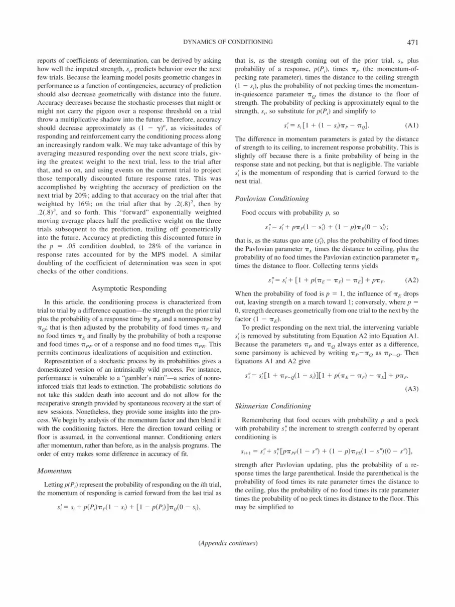
reports of coefficients of determination, can be derived by askinghow well the imputed strength, si, predicts behavior over the nextfew trials. Because the learning model posits geometric changes inperformance as a function of contingencies, accuracy of predictionshould also decrease geometrically with distance into the future.Accuracy decreases because the stochastic processes that might ormight not carry the pigeon over a response threshold on a trialthrow a multiplicative shadow into the future. Therefore, accuracyshould decrease approximately as (1 � �)n, as vicissitudes ofresponding and reinforcement carry the conditioning process alongan increasingly random walk. We may take advantage of this byaveraging measured responding over the next score trials, giv-ing the greatest weight to the next trial, less to the trial afterthat, and so on, and using events on the current trial to projectthose temporally discounted future response rates. This wasaccomplished by weighting the accuracy of prediction on thenext trial by 20%; adding to that accuracy on the trial after thatweighted by 16%; on the trial after that by .2(.8)2, then by.2(.8)3, and so forth. This “forward” exponentially weightedmoving average places half the predictive weight on the threetrials subsequent to the prediction, trailing off geometricallyinto the future. Accuracy at predicting this discounted future inthe p � .05 condition doubled, to 28% of the variance inresponse rates accounted for by the MPS model. A similardoubling of the coefficient of determination was seen in spotchecks of the other conditions.

Asymptotic Responding

In this article, the conditioning process is characterized fromtrial to trial by a difference equation—the strength on the prior trialplus the probability of a response time by �P and a nonresponse by�Q; that is then adjusted by the probability of food times �F andno food times �E and finally by the probability of both a responseand food times �PF or of a response and no food times �PE. Thispermits continuous idealizations of acquisition and extinction.

Representation of a stochastic process by its probabilities gives adomesticated version of an intrinsically wild process. For instance,performance is vulnerable to a “gambler’s ruin”—a series of nonre-inforced trials that leads to extinction. The probabilistic solutions donot take this sudden death into account and do not allow for therecuperative strength provided by spontaneous recovery at the start ofnew sessions. Nonetheless, they provide some insights into the pro-cess. We begin by analysis of the momentum factor and then blend itwith the conditioning factors. Here the direction toward ceiling orfloor is assumed, in the conventional manner. Conditioning entersafter momentum, rather than before, as in the analysis programs. Theorder of entry makes some difference in accuracy of fit.

Momentum

Letting p(Pi) represent the probability of responding on the ith trial,the momentum of responding is carried forward from the last trial as

s�i � si � p�Pi��P�1 � si� � �1 � p�Pi���Q�0 � si�,

that is, as the strength coming out of the prior trial, si, plusprobability of a response, p(Pi), times �P (the momentum-of-pecking rate parameter), times the distance to the ceiling strength(1 � si), plus the probability of not pecking times the momentum-in-quiescence parameter �Q times the distance to the floor ofstrength. The probability of pecking is approximately equal to thestrength, si, so substitute for p(Pi) and simplify to

s�i � si �1 � �1 � si��P � �Q�. (A1)

The difference in momentum parameters is gated by the distanceof strength to its ceiling, to increment response probability. This isslightly off because there is a finite probability of being in theresponse state and not pecking, but that is negligible. The variables�i is the momentum of responding that is carried forward to thenext trial.

Pavlovian Conditioning

Food occurs with probability p, so

s �i � s�i � p�F�1 � s�i� � �1 � p��E�0 � s�i�;

that is, as the status quo ante (s�i), plus the probability of food timesthe Pavlovian parameter �F times the distance to ceiling, plus theprobability of no food times the Pavlovian extinction parameter �E

times the distance to floor. Collecting terms yields

s �i � s�i � �1 � p��E � �F� � �E� � p�F. (A2)

When the probability of food is p � 1, the influence of �E dropsout, leaving strength on a march toward 1; conversely, where p �0, strength decreases geometrically from one trial to the next by thefactor (1 � �E).

To predict responding on the next trial, the intervening variables�i is removed by substituting from Equation A2 into Equation A1.Because the parameters �P and �Q always enter as a difference,some parsimony is achieved by writing �P��Q as �P�Q. ThenEquations A1 and A2 give

s �i � s�i �1 � �P�Q�1 � si���1 � p��E � �F� � �E� � p�F.

(A3)

Skinnerian Conditioning

Remembering that food occurs with probability p and a peckwith probability s�, the increment to strength conferred by operantconditioning is

si 1 � s�i � s�i �p�PF�1 � s�� � �1 � p��PE�1 � s���0 � s���,

strength after Pavlovian updating, plus the probability of a re-sponse times the large parenthetical. Inside the parenthetical is theprobability of food times its rate parameter times the distance tothe ceiling, plus the probability of no food times its rate parametertimes the probability of no peck times its distance to the floor. Thismay be simplified to

(Appendix continues)

471DYNAMICS OF CONDITIONING

si 1 � s�i �1 � �1 � s�i ��p�PF � �1 � p�s�i�PE��. (A4)

Inserting Equation A3 into this gives the final equation ofprediction, too unenlightening to be written out here— eventhough it is less complicated than the full solution to the R-Wmodel (Yamaguchi, 2006). It is simpler to evaluate Equation A3and then insert it into Equation A4. A spreadsheet for analyzingdata with the present theory on a trial-by-trial basis is availablefrom Peter R. Killeen, Federico Sanabria, and Igor Dolgov.

Special Cases

Acquisition

In the case of acquisition, where few or no responses have yetoccurred, Equation A3 provides a good equation of prediction.Because the probability of food p is typically 1.0, it can be furthersimplified to the acquisition function

si 1 � si �1 � �P�Q�1 � si�� �1 � �F� � �F. (A5)

Equation A5 can range from a classic exponential-integral learn-ing curve (when �P�Q is of small magnitude) through approxi-mately linear to an S-shaped ogive, depending on the two param-eters, the net rate of persistence (�P�Q) and the rate of acquisition(�F).

Extinction

In extinction, p � 0, and Equation A3 simplifies to

si 1 � si�1 � �E��1 � �P�Q�1 � si��, (A6)

which appears as Equation 8 in the text. Equation A6 assumesthat �PE is smaller and that extinction decrements can behandled by �E; this has been the case for all of the dataanalyzed here, and setting �E to zero is a parsimonious way tosimplify the equation.

Received April 15, 2008Revision received February 6, 2009

Accepted February 6, 2009 �

New Editors Appointed, 2011–2016

The Publications and Communications Board of the American Psychological Association an-nounces the appointment of 3 new editors for 6-year terms beginning in 2011. As of January 1,2010, manuscripts should be directed as follows:

● Developmental Psychology (http://www.apa.org/journals/dev), Jacquelynne S. Eccles, PhD,Department of Psychology, University of Michigan, Ann Arbor, MI 48109

● Journal of Consulting and Clinical Psychology (http://www.apa.org/journals/ccp), Arthur M.Nezu, PhD, Department of Psychology, Drexel University, Philadelphia, PA 19102

● Psychological Review (http://www.apa.org/journals/rev), John R. Anderson, PhD, Depart-ment of Psychology, Carnegie Mellon University, Pittsburgh, PA 15213

Electronic manuscript submission: As of January 1, 2010, manuscripts should be submittedelectronically to the new editors via the journal’s Manuscript Submission Portal (see the websitelisted above with each journal title).

Manuscript submission patterns make the precise date of completion of the 2010 volumesuncertain. Current editors, Cynthia Garcıa Coll, PhD, Annette M. La Greca, PhD, and Keith Rayner,PhD, will receive and consider new manuscripts through December 31, 2009. Should 2010 volumesbe completed before that date, manuscripts will be redirected to the new editors for considerationin 2011 volumes.

472 KILLEEN, SANABRIA, AND DOLGOV