THE ECONOMIC IMPACT OF RESTRICTED WATER SUPPLY: A COMPUTABLE GENERAL EQUILIBRIUM ANALYSIS Maria Berrittellaa, Arjen Y. Hoekstrab, Katrin Rehdanzc, Roberto Rosond,e and Richard S.J. Tolc,f,g,h,*

a Centro Interdipartimentale di Ricerche sulla Programmazione Informatica dell’Economia e delle Tecnologie (CIRPIET), University of Palermo, Palermo, Italy b Department of Water Engineering and Management, University of Twente, Enschede, Netherlands c Research Unit Sustainability and Global Change, Hamburg University and Centre for Marine and Atmospheric Science, Hamburg, Germany d Department of Economics, University Ca’ Foscari, Venice, Italy e Fondazione Eni Enrico Mattei, Venice, Italy f Economic and Social Research Institute, Dublin, Ireland

g Institute for Environmental Studies, Vrije Universiteit, Amsterdam, The Netherlands h Engineering and Public Policy, Carnegie Mellon University, Pittsburgh, PA, USA Working Paper FNU-93 (revised) Abstract Water problems are typically studied at the level of the river catchment. About 70% of all water is used for agriculture, and agricultural products are traded internationally. A full understanding of water use is impossible without understanding the international market for food and related products, such as textiles. The water embedded in commodities is called virtual water. Based on a general equilibrium model, we offer a method for investigating the role of water resources and water scarcity in the context of international trade. We run five alternative scenarios, analysing the effects of water scarcity due to reduced availability of groundwater. This can be a consequence of physical constraints, and of policies curbing water demand. Four scenarios are based on a “market solution”, where water owners can capitalize their water rent or taxes are recycled. In the fifth “non-market” scenario, this is not the case; supply restrictions imply productivity losses. Restrictions in water supply would shift trade patterns of agriculture and virtual water. These shifts are larger if the restriction is larger, and if the use of water in production is more rigid. Welfare losses are substantially larger in the non-market situation. Water-constrained agricultural producers lose, but unconstrained agricultural produces gain; industry gains as well. As a result, there are regional winners and losers from water supply constraints. Because of the current distortions of agricultural markets, water supply constraints could improve allocative efficiency; this welfare gain may more than offset the welfare losses due to the resource constraint. Keywords: Computable General Equilibrium, Sustainable Water Supply, Virtual Water, Water Scarcity JEL Classification: D58, Q25, Q28 1 Introduction

1

Water is one of our basic resources, but it is often short. Estimates have shown that the total amount of water available would be sufficient to provide the present world population only with a minimum amount of freshwater required. However, the uneven distribution of water (and population) among regions has made the adequate supply critical for a growing number of countries. A rapid population growth and an increasing consumption of water per capita has aggravated the problem. This tendency is likely to continue as water consumption for most uses is projected to increase by at least 50% by 2025 compared to 1995 level (Rosegrant et al. 2002). One additional reason for concern is (anthropogenic) climate change, which may lead to increased drought in many places (IPCC, 2001). Water problems are typically defined and studied at the level of the river catchment, if not at a finer spatial scale. This is a valid approach for many applications. Yet, 70% of all water is used for agriculture, and agricultural products are traded internationally. A complete understanding of water use is therefore impossible without understanding the international markets for food and other agriculture related products, such as textiles. This study offers a method of studying the role of water resources and water scarcity in the context of international trade. Previous studies have introduced the term “virtual water” to indicate the implicit water content of internationally traded commodities. Virtual water is the water used in production, rather than the water contained in the product, and virtual water export (import) is the water used to produce exported (imported) goods (Allan, 1992, 1993). Water contained in the product is a fraction of the water used in production. For example, Chapagain and Hoekstra (2004) calculate a global virtual water flow of 16% of total global water use. However, these studies are descriptive: virtual water flows are estimated, but changes in either water resources or economic circumstances cannot be readily assessed. In contrast, our model allows for the analysis of virtual water flows for many scenarios, within a framework consistent with economic theory. Furthermore, the model belongs to a class of empirical tools (CGE) which has been extensively used for trade liberalization, development, and fiscal policy analysis. Other studies, notably Rosegrant et al. (2002), use partial equilibrium models for scenario studies. Our general equilibrium approach allows for a richer set of economic feedbacks and for a complete assessment of welfare implications, but this of course comes at the price of a cruder resolution. The analysis is based on countries’ total renewable water resources and differences in water productivity. For example, we account for the fact that growing wheat in North African countries requires more water than growing it in the USA. Also, different crop types have different water requirements: the production of a ton of rice is more water intensive than the production of a ton of wheat. Within the GTAP regions, we use the crop-value-weighted average of national estimates. In this paper, we present a computable general equilibrium model, especially designed to account for water resources (GTAP-W), and illustrate its potential application for sustainable water supply uses. Section 2 reviews the literature, highlighting the original contribution of our model, which appears to be truly the first global, multi-regional, multi-sectoral trade model with virtual water flows and water as a factor of production. The model is a first step in improving our understanding of the interactions between water resource and international trade in agricultural products. Because the temporal and spatial resolution is course, and the data are crude, the model cannot be used directly for advice on water policy. Section 3 presents the model and the data on water resources and use, and discusses the limitations of the data and the model. The basic model and economic data are derived from the Global Trade and Analysis Project (http://www.gtap.agecon.purdue.edu/). The water satellite accounts can be found at:

http://www.fnu.zmaw.de/GTAP-EF-W.5680.0.html

2

Section 4 discusses five alternative scenarios. Section 5 analyses the results. Section 6 discusses and concludes. 2 Previous studies As the supply of water is limited, attempts have been made to economize on the consumption of water, especially in regions where the supply is critical (Seckler et al., 1998; Dinar and Yaron, 1992). However, in many regions water is subsidized (Rosegrant et al., 2002). An alternative strategy to meet the increasing demand for water is the desalination of brackish or sea water (Ettouney et al., 2002; Zhou and Tol, 2005). Another possibility to minimize water use in water-short countries is to increase imports of products that require a lot of water in their production. The water embedded in commodities is also called virtual water (Allan, 1992, 1993). We use the production site definition, that is, we consider the actual water used in production. The virtual water content of a product can also be defined as the volume of water that would have been required to produce the product in the place where it is consumed (consumption site specific definition). A recent study by the UNESCO-IHE Institute for Water Education on global virtual water trade, for the period 1997-2001, revealed that in order to produce e.g. one ton of husked rice, on average 3,000 m3 of virtual water are necessary; this is the world average; the number varies from 1,600 m3 per tonne in Japan and the USA to 4,000 m3 per tonne in Brazil (see Chapagain and Hoekstra, 2004; see also Hoekstra and Hung,2003, 2005 and Chapagain and Hoekstra, 2003). For livestock products the numbers are much higher. Due to differences in climate conditions and animal diets, the water use numbers differ significantly between countries. Other studies may have different numbers for particular crops or particular countries. The main advantage of using the Chapagain and Hoekstra (2004) data is that it covers all crops and all countries in an internally consistent way. According to Chapagain and Hoekstra (2004), 61% of the global virtual water trade is related to international trade in crops, 17% is related to trade in livestock and livestock products and only 22% is related to trade in industrial products. In total, 16% of water used in the world for agricultural and industrial production is exported as virtual water. Countries like the US, Canada, Australia, Argentina and Thailand are the biggest net exporters of virtual water, whereas Japan, Italy, UK, Germany and South Korea are the biggest net importers. If these figures are weighted against a country’s endowment of water resources the picture is quite different. In relative terms, countries in the Middle East and North Africa import a lot of virtual water. On the other hand, USA, Canada, South America and Australia are exporting a significant share of their water resources. As the water requirement for food production is large, virtual water might be seen as an additional source of water for water-scarce countries. Indeed, much of the existing literature stresses the political relevance and emphasizes the role of virtual water in providing food security in water-short regions (Bouwer, 2000; Allan and Olmsted, 2003). Some researchers have even argued that virtual water trade could perhaps prevent wars over water (Allan, 1997; Homer-Dixon, 1994, would disagree). Others fear that regions become dependent on global trade and vulnerable to market fluctuations. However, most countries have no explicit strategy for virtual water trade (Yang and Zehnder, 2002). Another branch of the literature has compared the concept of virtual water trade to the economic concept of comparative advantages (see e.g. Wichelns, 2001, 2004; Hakimian, 2003), but the data show little correlation between the virtual water trade balance and water endowments (Wichelns, 2004; Ramirez-Vallejo and Rogers, 2004), probably because water is usually not (fully) priced. Although the concept of virtual water trade is appealing, the number of empirical studies is limited. Renault (2003) and Zimmer and Renault (2003) provide estimates on global virtual

3

water trade, one by the World Water Council (WWC), in collaboration with the FAO (Food and Agricultural Organization of the United Nation); see Oki et al. (2003). Although different in data and methodology, results are close to the ones obtained by the UNESCO-IHE. Others have investigated why the virtual water trade balance is positive for some countries and negative for others. Yang et al. (2003) found evidence that virtual water import for cereals increases with decreasing water resources. Hoekstra and Hung (2003, 2005) compared water scarcity and water dependency and found perhaps unexpected results for some countries: There is no relationship between national water scarcity and virtual water trade. One aspect, which has not attracted much attention so far are changes in virtual water trade over time. Yang et al. (2003) used population predictions to calculate the annual water deficit for water-scarce countries by 2030. Calculations are based on cereal imports. Unsurprisingly, they found an exponential increase. Rosegrant et al. (2002) used the IMPACT-WATER model to estimate demand and supply of food and water to 2025. Scenarios for water demand and supply to 2025 are provided by Seckler et al. (1998). A detailed analysis of the world water situation by 2025 is given by Alcamo et al. (2000). In their most recent paper, Rosegrant et al. (2002) include virtual water trade, using cereals as an indicator (Fraiture et al., 2004). Their results suggest that the role of virtual water trade is modest, but these findings have been obtained in a partial equilibrium analysis, in which non-agricultural sectors are mainly excluded. Although most water is used in agriculture, shifts in agriculture would affect other sectors, both domestically and internationally. Studies using general equilibrium approaches typically focus on a single country or region. Decaluwe et al. (1999) analyze the effect of water pricing policies on demand and supply of water in Morocco. Daio and Roe (2003) use an intertemporal CGE model for Morocco, analyzing water and trade policies. For the Arkansas River Basin, Goodman (2000) shows that temporary water transfers are less costly than building new dams. Gómez et al. (2004) analyze the welfare gains of improved allocation of water rights in the Balearic Islands. These studies have an explicit representation of water as a factor of production. Other studies use agricultural productivity (e.g., Horridge et al., 2005) or land use as a proxy for water (e.g., Seung et al., 2000). Letsoalo et al. (forthcoming) treat water as a cost factor only. Our analysis is different. In this paper, we include water as an endowment in the production structure of the economy. We use a computable general equilibrium model of the world economy to analyze the implications of reduced supply of water in water-scarce countries. Reduced water supply necessarily implies that the relative price of water-intensive products would increase, that the relative competitiveness of all industries would change, and that the terms of trade of all regions would shift, presumably to the benefit of water-abundant regions. By focusing on single sectors or countries, the above studies do not consider this. We consider various scenarios, and study the effects on virtual water flows, international trade, and welfare. As the literature review above indicates, we are the first to do this. Therefore, our results cannot be compared to earlier model studies. Nor can our work be compared to empirical work, as the wider economic implications of restrictions in water supply have not been estimated. We present our data and model in the next section. Because of lack of data, we were unable to distinguish between rainfed and irrigated agriculture. For the same reason, we were unable to allow the agents to substitute away from water in production, although they are of course able to substitute away from water-intensive products. The paper should be seen as a first step. 3 Modeling framework and data

4

In order to assess the systemic general equilibrium effects of restricted water supply, we use a multi-region world CGE model, called GTAP-W. The model is a refinement of the GTAP model. The GTAP model is a standard CGE static model distributed with the GTAP database of the world economy. For detailed information see Hertel (1997) and the technical references and papers available on the GTAP website (www.gtap.org). We use the GTAP-E version modified by Burniaux and Truong (2002). The GTAP variant developed by Burniaux and Truong (2002) is best suited for the analysis of energy markets and environmental policies. There are two main changes in the basic structure. First, energy factors are separated from the set of intermediate inputs and inserted in a nested level of substitution with capital. This allows for more substitution possibilities. Second, database and model are extended to account for CO2 emissions related to energy consumption. Basically, in the GTAP-W model a finer industrial and regional aggregation level, respectively, 17 sectors (6 of which in agriculture and forestry) and 16 regions, is considered, and water resources, as non-marketed goods, have been modeled. See Annex Table A1 for the regional, sectoral and factor aggregations used in GTAP-W, some characteristics are given in Table A2. The model is based on 1997 data. The crude regional and sectoral resolution make that the quantitative insights of this paper are limited; the contribution of this paper is qualitative and methodological. As in all CGE models, the GTAP-W model makes use of the Walrasian perfect competition paradigm to simulate adjustment processes. Industries are modeled through a representative firm, which maximizes profits in perfectly competitive markets. The production functions are specified via a series of nested CES functions (Figure A1 and Table A3 in Annex). Domestic and foreign inputs are not perfect substitutes, according to the so-called "Armington assumption", which accounts for product heterogeneity. A representative consumer in each region receives income, defined as the service value of national primary factors (natural resources, land, labour and capital). Capital and labour are perfectly mobile domestically, but immobile internationally. Land (imperfectly mobile) and natural resources are industry-specific. The national income is allocated between aggregate household consumption, public consumption and savings (Figure A2 in Annex). The expenditure shares are generally fixed, which amounts to saying that the top level utility function has a Cobb-Douglas specification. Private consumption is split in a series of alternative composite Armington aggregates. The functional specification used at this level is the Constant Difference in Elasticities (CDE) form: a non-homothetic function, which is used to account for possible differences in income elasticities for the various consumption goods. A money metric measure of economic welfare, the equivalent variation, can be computed from the model output. In the GTAP model and its variants, two industries are treated in a special way and are not related to any region. International transport is a world industry, which produces the transportation services associated with the movement of goods between origin and destination regions, thereby determining the cost margin between f.o.b. and c.i.f. prices. Transport services are produced by means of factors submitted by all countries, in variable proportions. In a similar way, a hypothetical world bank collects savings from all regions and allocates investments so as to achieve equality of expected future rates of return. In our modeling framework, water is combined with the value-added-energy nest and the intermediate inputs as displayed in Figure A1 (Annex). As in the original GTAP model, there is no substitutability between intermediate inputs and value-added for the production function of tradable goods and services. Therefore, a price-induced drop in water demand does not imply an increase in any other input. That is, water is a factor of production, but not a substitutable one. In the benchmark equilibrium, water supply is supposed to be unconstrained, so that water demand is lower than water supply, and the price for water is zero. Water is supplied to the agricultural industry, which includes primary crop production

5

and livestock, and to the water distribution services sector, which delivers water to the rest of the economic sectors. Note that distributed water can have a price, even if primary water resources are in excess supply. Furthermore, water is mobile between the different agricultural sectors. However, water is immobile between agriculture and the water distribution services sector, because the water treatment and distribution is very different between agricultural and other uses. We change this assumption in a sensitivity analysis. The key parameter for the determination of regional water use is the water intensity coefficient. This is defined as the amount of water necessary for sector j to produce one unit of commodity. This refers to water directly used in the production process, not to the water indirectly needed to produce other input factors. To estimate water intensity coefficients, we first calculated total water use by commodity and country for the year 1997. For the agricultural sector the FAOSTAT database provided information on production of primary crops and livestock. This includes detailed information on different crop types and animal categories. Information on water requirements for crop growth and animal feeding was taken from Chapagain and Hoekstra (2004). This information is provided as an average over the period from 1997 to 2001. The CGE is calibrated for 1997. The water requirement includes both the use of blue water (ground and surface water) as well as green water (moisture stored in soil strata). For crops it is defined as sum of water needed for evapotranspiration, from planting to harvest, and depends on crop type and region. This procedure assumes that water is not short and no water is lost by irrigation inefficiencies. For animals, the virtual water content is mainly the sum of water needed for feeding and drinking. The water intensity parameter for the water distribution sector is based on the country’s industrial and domestic water use data provided by AQUASTAT. This information is based on data for 2000. By making use of this data we assume that domestic and industrial water uses in 2000 are the same as in 1997. The data we use are imperfect. Water use by crop is uncertain, variable, and estimated with a rough methodology; Chapagain and Hoekstra (2004) do not distinguish between rainfed and irrigated agriculture. The AQUASTAT database has similar problems for water use, as well as for water resources. The FAOSTAT database on crop production has a mix of high and low quality data. Nonetheless, there are no databases with equal coverage, both in countries and in crop detail, and higher quality. The mechanism through which water scarcity is introduced into the model is the potential emergence of economic rents associated with water resources. If supply falls short of demand, consumers would be rationed, and willing to pay a price to access to water, because water has an economic value, as it is needed in production. If water resources are privately or collectively owned, the owners receive an economic rent, which becomes a component of available income. The price for water is then set by the market at the level that makes water demand compatible with supply. In this setting, water supply is assumed to be completely inelastic (vertical). By introducing technologies for “effective” water production, the supply function could, however, be positively sloped. Therefore, we introduce a constraint on water amounts, in our model, which entails the creation of a new market and a new exchangeable commodity. Finally, we make the link between output levels and water demand sensitive to water prices. In other words, we assume that more expensive water brings about rationalization in usage and substitution with other factors. The capability of reducing the relative intensity of water demand is industry-specific, and captured by a sector- and region-specific parameter (see Table 1). Note that the parameters are little more than informed guesses, derived from Rosegrant et al. (2002). We report a sensitivity analysis below. Details are given in Appendix B.

Table 1 about here

6

4. Design of simulation exercises We run five alternative simulation exercises, all dealing with the economic impacts of restricted water supply. In particular, we deny the use of groundwater as a source of water. There are two possible, alternative interpretations. First, regulators can decide that groundwater should not be pumped faster than it is replenished. Second, groundwater resources can run dry. Pumping groundwater from aquifers at a rate faster than it replenishes clearly violates sustainability constraints. We subtract the excess use of groundwater from the total amount of available water resources by country (assumed to be equal to water demand in the calibration year), as specified by FAO’s AQUASTAT database. Also, we add sustainable water resources per basin, as specified by Rosegrant et al. (2002). It turns out that water supply would be restricted in four regions: North Africa (NAF), South Asia (SAS), United States (USA) and China (CHI). In the first four scenarios, we consider the “market mechanism” to the problem of water scarcity. In the first scenario, NAF is the region with the greatest assumed decrease in water supply, facing a shortage of 10%. For the other regions, the water supply constraints are less substantial. In SAS and USA, water supply is assumed to decrease by 1.58%, and in CHINA by 3.92%.1 Scenario 2 can be regarded as an example of what would happen to an economy when sustainable water supply policies are delayed, and unexpected and severe shortages in water availability occur. In this scenario, NAF faces an instantaneous shortage of 44%; (the water supply constraints in the other regions do not change). Scenarios 3 and 4 are both variants of scenario 1. In scenario 3, we assume that water is specific to each agricultural sector, that is, water is not mobile between the agricultural sectors. In scenario 4, water use is not sensitive to the price. The main limitation of the market approach is given by the implicit assumption that property rights on water resources can be defined and enforced, which is not always the case. Rights to irrigation water may be explicit, but rights to rainwater are an implicit part of land title. Water rights and land titles are not necessarily secure, and capital markets are not accessible to all. For this reason, in scenario 5, we provide an alternative mechanism that does not require the creation of a competitive market. When water gets scarce, but there is no way of buying more water on the market, the main effect will be a reduction of production for the same level of non-water factor inputs. This is equivalent to a drop in productivity in water demanding industries. The fall in productivity also makes produced goods more expensive, reducing their demand and, indirectly, that for water.2 This scenario uses the same constraints as in scenario one. There is an alternative interpretation. Above, we assume that the water supply is constrained. In the market scenarios (1-4), the water users can reap the increase in rent due to the restriction on the resources; in the non-market scenario (5), the water users cannot use this rent, for instance because water property rights are implicit and cannot be used as assets on the capital market. In the alternative interpretation, the regulator restricts water supply by imposing a tax. In scenarios 1-4, the tax is recycled to the water users proportional to their water use, but lump sum. An individual water user can control her water use, and hence her total water charge; however, the tax rebate depends on all water users and is beyond the 1 The reduction is water supply is small relative to the annual variation in precipitation. However, GTAP-W is a static computable general equilibrium model. The reductions in water supply are reductions in the long-term, average water supply. 2 Note that in this construction, the extent of technological regress is endogenous, and therefore only implicitly determined by the water supply constraint. That is, the change in water supply is real, the change in productivity only a derivative.

7

control of an individual water user. Under these assumptions, the tax is neutral in the government budget, and the ratio of private to public consumption is preserved. In scenario 5, the tax money is not recycled. Economically, and in our model, the two interpretations are equivalent: “restricted water supply plus higher water rents” equals “water tax plus lump sum recycling” (scenarios 1-4); “restricted water supply but no higher water rents” equals “water tax without recycling” equals “reduction of land productivity” (scenario 5). The interpretations are not the same from an environmental policy perspective; in the first interpretation, the water is not there; in the second interpretation, the water is there but cannot be used by humans. Note that the data combine rainfall and irrigation water. For irrigation water, it is straightforward to picture water rights and water rents. For rainfall, the property right on water is implicitly captured by the property right on the land on which the rain falls. If water would be scarcer, the value of both irrigation water and rainfall would increase. This water rent would express itself as an increase in the value of water rights in the case of irrigated agriculture; and as an increase in the value of land in the case of rainfed agriculture. See Mendelsohn et al. (1994) and Schlenker et al. (2005) for empirical evidence. 5 Simulation results Results for all scenarios described in section 4 are presented in Tables 2 to 7. The tables report values for some key economic variables: water demand, water rent, virtual water trade balance, trade balance, welfare indexes. Scenario 1 is our base scenario; comparison is done to scenario 1; scenario 1 is compared to the situation without restrictions on water supply. In scenario 1, reported in Table 2, we simulate water reductions in NAF, CHI, USA and SAS. The difference in water rent between agriculture and the water distribution services is due to the fact that water distribution is much more responsive to price changes than the agricultural sector (see Table 1). Note that, although USA and SAS face the same water supply constraint, water prices are higher in the USA (0.9 Cent per m3 versus 0.5 Cent per m3). However, SAS uses almost twice the amount of water in the baseline compared to the USA (compare Table A2 in the Appendix). Also, CHI has a significant lower water supply constraint than NAF, but its water rent is higher (3 Cent per m3) than in NAF (0.5 Cent per m3). These differences cannot be explained in terms of differences in water price sensitivity (see Table 1). Nonetheless, there are two ways to reduce the amount of water demand: reducing water in water-demanding industries, and reducing demand for goods produced with water. This latter, indirect water demand reduction may be achieved in two ways: substitution in production and consumption with other goods, and substitution with goods of the same type, but produced abroad. Additional imports, however, require an expansion of exports in other industries and/or an increase of foreign direct investments. Results suggest that this indirect demand reduction is the primary determinant of prices in water markets.

Table 2 about here In terms of virtual water trade, as expected, less water supply leads to an increase in virtual water import in the constrained regions, and to a decrease in virtual water exports. This is due to the relatively more expensive production of water intensive goods and services in the constrained regions. Water-short countries can meet their demand of water-intensive products by importing them (Bouwer, 2000; Allan and Olmsted, 2003). On the other hand, a deficit in terms of virtual water trade is not always accompanied by a negative variation in the trade balance. For example, in NAF, SAS and CHI the trade balance improves.

8

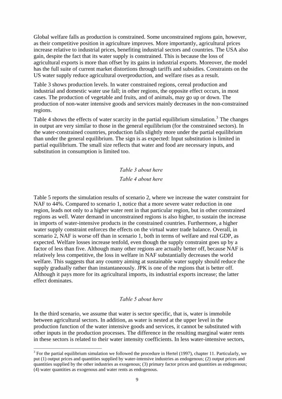
Global welfare falls as production is constrained. Some unconstrained regions gain, however, as their competitive position in agriculture improves. More importantly, agricultural prices increase relative to industrial prices, benefiting industrial sectors and countries. The USA also gain, despite the fact that its water supply is constrained. This is because the loss of agricultural exports is more than offset by its gains in industrial exports. Moreover, the model has the full suite of current market distortions through tariffs and subsidies. Constraints on the US water supply reduce agricultural overproduction, and welfare rises as a result. Table 3 shows production levels. In water constrained regions, cereal production and industrial and domestic water use fall; in other regions, the opposite effect occurs, in most cases. The production of vegetable and fruits, and of animals, may go up or down. The production of non-water intensive goods and services mainly decreases in the non-constrained regions. Table 4 shows the effects of water scarcity in the partial equilibrium simulation.3 The changes in output are very similar to those in the general equilibrium (for the constrained sectors). In the water-constrained countries, production falls slightly more under the partial equilibrium than under the general equilibrium. The sign is as expected: Input substitution is limited in partial equilibrium. The small size reflects that water and food are necessary inputs, and substitution in consumption is limited too.

Table 3 about here Table 4 about here

Table 5 reports the simulation results of scenario 2, where we increase the water constraint for NAF to 44%. Compared to scenario 1, notice that a more severe water reduction in one region, leads not only to a higher water rent in that particular region, but in other constrained regions as well. Water demand in unconstrained regions is also higher, to sustain the increase in imports of water-intensive products in the constrained countries. Furthermore, a higher water supply constraint enforces the effects on the virtual water trade balance. Overall, in scenario 2, NAF is worse off than in scenario 1, both in terms of welfare and real GDP, as expected. Welfare losses increase tenfold, even though the supply constraint goes up by a factor of less than five. Although many other regions are actually better off, because NAF is relatively less competitive, the loss in welfare in NAF substantially decreases the world welfare. This suggests that any country aiming at sustainable water supply should reduce the supply gradually rather than instantaneously. JPK is one of the regions that is better off. Although it pays more for its agricultural imports, its industrial exports increase; the latter effect dominates.

Table 5 about here In the third scenario, we assume that water is sector specific, that is, water is immobile between agricultural sectors. In addition, as water is nested at the upper level in the production function of the water intensive goods and services, it cannot be substituted with other inputs in the production processes. The difference in the resulting marginal water rents in these sectors is related to their water intensity coefficients. In less water-intensive sectors, 3 For the partial equilibrium simulation we followed the procedure in Hertel (1997), chapter 11. Particularly, we put (1) output prices and quantities supplied by water-intensive industries as endogenous; (2) output prices and quantities supplied by the other industries as exogenous; (3) primary factor prices and quantities as endogenous; (4) water quantities as exogenous and water rents as endogenous.

9

such as animal husbandry, the marginal water rents rise more than in scenario 1 (see Table 6). Animal husbandry needs less water per unit of output than do crops. The price increase is particularly pronounced for NAF with a water price of $63 per m3 of water for a 10% fall in water supply, four orders of magnitude higher than in the previous scenarios. This follows from the fact that water is already used very efficiently in this sector and region, while demand is inelastic. Note that the water price is still only six cent per litre. In general, NAF, SAS and CHI import more virtual water than in scenario 1. Furthermore, they shift their domestic production to water-extensive goods and services, which also increases imports of such goods, leading to gains in the terms of trade. Compared to scenario 1, the restriction of the water mobility increases slightly the competitiveness of the other countries, resulting in a higher GDP. Immobile water resources lead to a lower loss of global welfare. This is surprising. The welfare of most regions is lower in scenario 3 than in scenario 1, as one would expect. The two main exceptions are WEU and JPK. Both regions improve their terms of trade, as industrial exports increase. Without water supply constraints, WEU also enjoys a competitive advantage in agriculture. Allocative welfare also improves in both regions, as regional and world prices for agricultural products converge. Note that global welfare in fact increases in scenario 3: the current agricultural economy is so distorted that a reduction in production improves welfare.

Table 6 about here Scenario 4 considers the same case as scenario 1, but the water intensity does not respond to the price of water price; that is, the water intensity parameters are the same between the base and the policy scenario in all sectors. This signifies less flexibility at the level of farms and water distribution companies. Water rents are higher than in scenario 1, and the difference is more pronounced in water price sensitive countries such as CHI and SAS, and, for the same reason, in the water distribution industry (see Table 7). Furthermore, as the constrained countries cannot improve their water efficiency in domestic production, they satisfy their demand of water-intensive products by increasing the imports more than in scenario 1, as the results in terms of virtual water trade indicate. NAF, CHI and SAS gain in terms of trade due to their increase of exports of water-extensive products. As the world welfare decreases in scenario 4 more than it does in scenario 1, the world would benefit from a policy, which leads to higher water efficiency.

Table 7 about here Scenario 5 is based on the “non-market” mechanism, that is, water users cannot reap the increase in resource rents or, equivalently, the water tax is not recycled. In this scenario, productivity is decreased so as to meet the water supply constraints, which are the same as in scenario 1. The resulting productivity changes differ between agriculture and water distribution services, and amongst the constrained regions (see Table 8). Productivity decreases faster in more water-intensive sectors than in scenario 1. The pattern of variations in the virtual water balance are as in scenario 1, but the absolute changes are greater. The global loss in welfare is considerably larger, even though some regions gain more. In the non-market scenario, each region with a supply constraint, including the USA, loses welfare.

Table 8 about here

10

6 Discussion and conclusion In this paper, we present a computable general equilibrium model of the world economy with water as an explicit factor of production. To an experienced CGE modeller, it should be known how to include an extra production factor – in principle. This paper contributes by doing this – in practice. Previously, this was not possible because the necessary data were missing – at least at the global scale, as water is a non-market good, not reported in national economic accounts. Earlier studies included water resources at the national or smaller scale. These studies necessarily miss the international dimension,4 which is important as water is implicitly traded in international markets, mainly for agricultural products. In our model, sector specific water resources are introduced as production factors in the agricultural sectors and the water distribution service sector. Water is mobile between the different agricultural sectors, but immobile between agriculture and the water distribution service sector (which delivers water to the rest of the economic sectors). As water is mainly required for agricultural production, we disaggregated agricultural production into five different sectors. This allows us to gain a wider insight into the implications of different water resource policies. In the model, water use is also country specific, as are water resources. This allows for differentiated responses, in which some countries specialise in water-intensive agricultural products. We illustrate the new model by studying the implications of increased water scarcity, with a particular focus on groundwater resources. Other applications can be thought of, and we are working on a number of them. The excess use of groundwater resources is an unambiguous example of future reductions in water supply, either through policy or through nature, as the reservoirs are depleted. Computable general equilibrium models are best at analysing structural economic change. In this case, the change is a regionally and sectorally differentiated fall in water supply. In the base scenario, we restrict water supply in some regions, but not in others. As expected, water use increases in the unconstrained regions as trade patterns shift; unconstrained regions produce and export more water-intensive products. The world as a whole is worse off, as production is constrained. However, some countries gain, as relative prices change. Interestingly, the USA is among the winners even though its water supply is constrained as well. This is partly due to distortionary subsidisation of agricultural production in the USA; water constraints temper the resulting overproduction. If water constraints are higher, so are welfare gains and losses; however, welfare gains respond less than proportionally, and welfare losses more than proportionally. Shifts in trade patterns are also larger. If water is less mobile, the economy has less ability to adapt, and water constraints have a more negative welfare impact in most regions. At the same time, regional welfare gains are more pronounced as well, so redistribution is amplified. In fact, the positive effects dominate the negative effects, so that global welfare increases; this is a sign that current agricultural markets are severely distorted. If water use is less flexible, the negative effects dominate. If water users cannot reap the higher rents induced by water scarcity (alternatively, if the government does not recycle the water tax), overall welfare losses are much higher, but again, so are the welfare gains in some of the regions that benefit. The USA, however, would be net losers in this scenario. Even though the physical input scenario is identical in 4 out of 5 scenarios, the realignment of agricultural trade is different in all cases; as a result, the actual water use is unique to each scenario. This analysis needs to be extended in several ways and a number of limitations apply. First, we have not been able to allocate industrial water use to its different users. We rather used a

4 Although, in a single country CGE, there is either an explicit “rest of the world” region or the rest of the world in implicitly included in the closure rules.

11

simplifying assumption that water for domestic and industry use is supplied by the water service sector. The price is the same for all industries (except agriculture). Second, we consider regional water supply, implicitly assuming that there is a perfect water market and costless water transport within each region. Sector-specific water resources allow for subregional differentiation of water resources, but only to a limited extent. Third, we were not able to differentiate between the different qualities of water supplied. Some of the difference is captured by defining sector-specific water, but not all. Fourth, in our model we assume that water is used efficiently and no water is wasted. The water intensity coefficient captures some differences, but these differences do not respond to price or other signals, except to the price of water. Fifth, for the agricultural sector, we used irrigation water plus rainfall, without distinction. Sixth, we nested water at the upper level in the production function of the water intensive goods and services, so that water cannot be substituted with specific inputs in the production processes. Seventh, we used a single data set for water use and water resources, ignoring the uncertainties in the data. All this is deferred to future research. Acknowledgements We had useful discussions about the topics of this paper with Francesco Bosello, Alvaro Calzadilla, Tom Hertel, Rob McDougall, Hom Pant, Jerry Shively, Wally Tyner, Jian Zhang and Yuan Zhou. Two anonymous referees, an anonymous associate editor, and Mark Horridge had useful comments on an earlier version of the paper. The paper was presented at EMF22 Land Use, Agricultural Economics Purdue U., Agricultural Economics U. Pretoria, QUEST U. Bristol, Economics U. Galway, 2005 GTAP Conference, 2005 EMF CCI/IA Workshop, Princeton Environmental Institute, International Food Policy Research Institute, DoA Economic Research Service, 3rd Workshop on Integrated Climate Models ICTP/Trieste and Otto Foundation; participants had many welcome comments. The Michael Otto Foundation for Environmental Protection provided welcome financial support. All errors and opinions are ours. References Alcamo, J., Henrichs, T. and Rösch, T. (2000) World water in 2025: Global modeling and

scenario analysis for the World Commission on Water for the 21st Century. Report A0002, Center for Environmental Systems Research, University of Kassel, Kassel, Germany.

Allan, J.A. (1992) Fortunately there are substitutes for water otherwise our hydro-political futures would be impossible. In: Proceedings of the Conference on Priorities for Water Resources Allocation and Management : Natural Resources and Engineering Advisers Conference, Southampton, July 1992, pp. 13-26.

Allan, J.A. (1993) Overall perspectives on countries and regions. In: Rogers, P. and Lydon, P. (Eds.) Water in the Arab World: Perspectives and Prognoses, Cambridge, Massachusetts, pp. 65-100.

Allan, J.A. (1997) ‘Virtual water’: A long term solution for water short Middle Eastern economies? Paper presented at the 1997 British Association Festival of Science, University of Leeds, 9 September.

Allan, J.A. and Olmsted, J.C. (2003) Politics, economics and (virtual) water: A discursive analysis of water policies in the Middle East and North Africa. Food, Agricultural, and Economic Policy in the Middle East and North Africa 5 53-78.

12

Bouwer, H. (2000) Integrated water management: Emerging issues and challenges. Agricultural Water Management 45 217-228.

Burniaux, J.-M. and Truong, T.P. (2002) GTAP-E: An energy environmental version of the GTAP model, GTAP Technical Paper n.16.

Chapagain, A.K. and Hoekstra, A.Y. (2003) Virtual water trade: A quantification of virtual water flows between nations in relation to international trade in livestock and livestock products. In Hoekstra, A.Y. (Ed.) Virtual water trade: Proceedings of the international expert meeting on virtual water trade, Delft, The Netherlands, 12-13 December 2002, pp. 49-76.

Chapagain, A.K. and Hoekstra, A.Y. (2004) Water Footprints of Nations, Value of Water Research Report Series No. 16, UNESCO-IHE Delft, The Netherlands.

Decaluwé, B., Patry, A. and Savard, L. (1999) When water is no longer heaven sent: Comparative pricing analysis in a AGE model, Working Paper 9908, CRÉFA 99-05, Départment d’économique, Université Laval.

Diao, X. and Roe, T. (2003) Can a water market avert the “double-whammy” of trade reform and lead to a “win-win” outcome? Journal of Environmental Economics and Management 45 708-723.

Dinar, A. and Yaron, D. (1992) Adoption and Abandonment of Irrigation Technologies. Agricultural Economics 6 315-32.

Ettouney, H.M., El-Dessouky, H.T., Faibish, R.S. and Gowin, P.J. (2002) Evaluating the Economics of Desalination. Chemical Engineering Progress, December 2002, pp. 32-39.

Fraiture, C. de, Cai, X., Amarasinghe, U., Rosegrant, M. and Molden, D. (2004) Does international cereal trade save water? The impact of virtual water trade on global water use. Comprehensive Assessment Research Report 4, Colombo, Sri Lanka.

Gómez, C.M., Tirado, D. and Rey-Maquieira, J. (2004) Water exchange versus water work: Insights from a computable general equilibrium model for the Balearic Islands, Water Resources Research 42 W10502 10.1029/2004WR003235.

Hakimian, H. (2003) Water scarcity and food imports: an empirical investigation of the ‘virtual water’ hypothesis in the MENA region. Review of Middle East Economics and Finance 1 (1) 71-85.

Goodman, D.J. (2000) More reservoir or transfer? A computable general equilibrium analysis of projected water shortages in the Arkansas River Basin, Journal of Agricultural and Resource Economics 25 (2) 698-713.

Hertel, T.W. (1997) Global Trade Analysis: Modeling and applications, Cambridge University Press, Cambridge.

Hoekstra, A.Y. and Hung, P.Q. (2003) Virtual water trade: A quantification of virtual water flows between nations in relation to international crop trade. In Hoekstra, A.Y. (Ed.) Virtual water trade: Proceedings of the international expert meeting on virtual water trade, Delft, The Netherlands, 12-13 December 2002, pp. 25-47.

Hoekstra, A.Y. and Hung, P.Q. (2005) Globalisation of water resources: international virtual water flows in relation to crop trade, Global environmental change 15 45-56.

Homer-Dixon, T.F. (1994) Environmental scarcities and violent conflict: Evidence from cases, International Securit, 19 (1), 5-40.

13

Horridge, M., Madden, J. and Wittwer, G. (2005)The impact of the 2002-2003 drought on Australia, Journal of Policy Modeling, 27, 285-308.

Intergovernmental Panel on Climate Change (2001) Impacts, adaptation, and vulnerability. Contribution of Working Group II to the Third Assessment Report of the Intergovernmental Panel on Climate Change Edited by McCarthy, J., Canziani, O., Leary, N., Dokken, D. and White, K., Cambridge University Press, Cambridge.

Letsoalo, A., J. Blignaut, T. de Wet, M. de Wit, S. Hess, R.S.J. Tol and J. van Heerden (forthcoming), Triple Dividends of Water Consumption Charges in South Africa, Water Resources Research.

Mendelsohn, R.O., Nordhaus, W.D. and Shaw, D. (1994), The Impact of Global Warming on Agriculture – A Ricardian Analysis, American Economic Review 84 (4), 753-771

Oki, T., Sato, M., Kawamura, A., Miyake, M., Kanae, S. and Musiake, K. (2003) Virtual water trade to Japan and in the world. In Hoekstra, A.Y. (Ed.) Virtual water trade: Proceedings of the international expert meeting on virtual water trade, Delft, The Netherlands, 12-13 December 2002, pp. 93-109.

Ramirez-Vallejo, J. and Rogers, P. (2004) Virtual Water Flows and Trade Liberalisation, Water Science and Technology, 49 (7), 25-32.

Renault, D. (2003) Virtual water in food: principles and virtues. In Hoekstra, A.Y. (Ed.) Virtual water trade: Proceedings of the international expert meeting on virtual water trade, Delft, The Netherlands, 12-13 December 2002, pp. 77-91.

Rosegrant, M.W., Cai, X. and Cline, S.A. (2002) World water and food to 2025: Dealing with scarcity. International Food Policy Research Institute, Washington, DC.

Schlenker, W., Hanemann, W.M. and Fisher, A.C. (2005) Will US Agriculture Really Benefit from Global Warming? Accounting for Irrigation in the Hedonic Approach, American Economic Review 95 (1) 395-406.

Seckler, D., Amarasinghe, U., Molden, D., Silve, R. de, Barker, R. (1998) World water demand and supply, 1990 to 2025: Scenarios and issues. Research Report 19. International Water Management Insitute, Colombo, Sri Lanka.

Seung, C.K., Harris, T.R., Eglin, J.E. and Netusil, N.R. (2000) Impacts of water reallocation: A combined computable general equilibrium and recreation demand model approach, The Annals of Regional Science 34 473-487.

Wichelns, D. (2001) The role of ‘virtual water’ in efforts to achieve food security and other national goals, with an example from Egypt. Agricultural Water Management 49 131-151.

Wichelns, D. (2004) The policy of virtual water can be enhanced by considering comparative advantages. Agricultural Water Management 66 49-63.

Yang, H., Reichert, P., Abbaspour, K.C. and Zehnder, A.J.B. (2003) A water resources threshold and its implications for food security. In Hoekstra, A.Y. (Ed.) Virtual water trade: Proceedings of the international expert meeting on virtual water trade, Delft, The Netherlands, 12-13 December 2002, pp. 111-116.

Yang, H. and Zehnder, A.J.B. (2002) Water scarcity and food import: A case study for southern Mediterranean countries. World Development 30 (8) 1413-1430.

Zhou, Y. and Tol, R.S.J. (2005) Evaluating the costs of desalination and water transport. Water Resource Research 41(3) W03003 10.1029/2004WR003749.

14

Zimmer, D. and Renault, D. (2003) Virtual water in food production and global trade: review of mythological issues and preliminary results. In Hoekstra, A.Y. (Ed.) Virtual water trade: Proceedings of the international expert meeting on virtual water trade, Delft, The Netherlands, 12-13 December 2002, pp. 93-109.

15

Annex A Table A1. Aggregations in GTAP-W

A. Regional Aggregation C. Sectoral Aggregation 1. USA - United States

2. CAN - Canada

3. WEU – Western Europe

4. JPK – Japan and Korea

5. ANZ – Australia and New Zealand

6. EEU – Eastern Europe

7. FSU – Former Soviet Union

8. MDE – Middle East

9. CAM – Central America

10. SAM – South America

11. SAS – South Asia

12. SEA – Southeast Asia

13. CHI - China

14. NAF – North Africa

15. SSA – Sub-Saharan Africa

16. ROW – Rest of the world

B. Endowments

1. Land

2. Labour

3. Capital

4. Natural Resource

1. Rice - Rice

2. Wheat - Wheat

3. CerCrops - Other cereals and crops

4. VegFruits - Vegetable, Fruits

5. Animals - Animals

6. Forestry - Forestry

7. Fishing – Fishing

8. Coal - Coal Mining

9. Oil – Oil

10. Gas - Natural Gas Extraction

11. Oil_Pcts - Refined Oil Products

12. Electricity – Electricity

13. Water - Water collection, purification and distribution services

14. En_Int_ind - Energy Intensive Industries

15. Oth_ind - Other industry and services

16. MServ - Market Services

17. NMServ - Non-Market Services

16

Table A2. Regional characteristics

Population GDP/cap Renewable water

resourcea Water use

Water intensity inagriculturec

Water intensity

otherd

Water imports

Water exports

mln $ 109m3

per year m3/personb109m3

per year m3/$ m3/$ 109m3 109m3

USA 276 28786 3069 11120 479 2.9 3.7 57 125CAN 30 20572 2902 96733 46 4.3 5.2 8 51WEU 388 24433 2227 5740 227 2.6 3.5 256 96JPK 172 35603 500 2907 107 1.4 1.6 82 0ANZ 22 21052 819 37227 26 4.1 1.2 3 30CEE 121 2996 494 4083 60 3.3 13.6 19 6FSU 291 1556 4730 16254 284 9.1 28.0 27 61MDE 227 3150 483 2128 206 4.9 6.8 35 19CAM 128 2938 1183 9242 101 5.2 13.6 25 31LAM 332 4830 12246 36886 164 3.9 5.9 35 68SAS 1289 416 3685 2859 918 9.8 47.5 21 25SEA 638 4592 5266 8254 279 10.1 12.8 58 35CHI 1274 790 2897 2274 630 3.6 38.5 33 16NAF 135 1284 107 793 95 8.5 39.5 27 4SSA 605 563 4175 6901 113 11.4 6.4 14 132ROW 42 3338 2984 71048 75 4.7 2.7 6 8

a 2001 estimates taken from Aquastat. b UN criterion for water resource scarcity degree: slightly scarce (1700-3000), middle scarce (1000-1700), severe scarcity (500-1000) and most severe scarcity (<500). c Average water intensity covering crop/plant growth and animal production measured in water use/$ output. Numbers differ considerably between countries and sectors. Note that water use includes the use of different kind of sources; rain, soil moisture and irrigation water. However, farmers pay for irrigation water only. d Note that in some countries only a low number of persons is connected to a distribution network. In others a number of self-supplied industries are not connected. However, both are included as users of the services the water distribution network provides. As a consequence, water use per $ of output is overstated in the above table.

17

Figure A1 – Nested tree structure for industrial production process

region 1 ……. region n region 1 ……. region n

foreign foreign foreign domestic domestic domestic

gas oil petroleum products

region 1 ……. region n

foreign domestic

coal non coal

region 1 ……. region n

region 1 ……. region n

foreigndomestic

non-electric electric

energy composite region 1 ……. region n capital

capital-energy composite foreign labour land natural resource domestic

value added (including energy inputs)

all other inputs (excluding energy inputs, but including energy feedstock)

water resource

outputσ=0

σVAE σD

σMσKE

σENER=1

σNELY=0.5

σNCOL=1

σD

σMσD

σM

σMσMσM

σD σD σD

18

Table A3. Substitution elasticities between different inputs

Sector σVAE(a) σΚΕ

(b) σD(c) σΜ

(d)

1. Rice 0.24 0.50 2.20 4.402. Wheat 0.24 0.50 2.20 4.403. Other cereals and crops 0.24 0.50 2.20 4.404. Vegetable, Fruits 0.24 0.50 2.20 4.405. Animals 0.24 0.50 2.80 5.606. Forestry 0.20 0.50 2.80 5.607. Fishing 0.20 0.50 2.80 5.608. Coal - Coal Mining 0.20 0.00 2.80 5.609. Oil 0.20 0.00 2.80 5.6010. Natural Gas Extraction 0.71 0.00 2.80 5.6011. Refined Oil Products 1.26 0.00 1.90 3.8012. Electricity 1.26 0.50 2.80 5.6013. Water collection, purification and distribution services 1.26 0.50 2.80 5.6014. Energy Intensive Industries 1.19 0.50 2.32 4.5715. Other industry and services 1.21 0.50 3.02 6.4016. Market Services 1.42 0.50 1.90 3.8017. Non-Market Services 1.26 0.50 1.90 3.80

(a) Substitution elasticity between land, natural resources, labour and capital-energy composite. (b) Substitution elasticity between capital and energy. (c) Substitution elasticity between domestic and imported inputs. (d) Substitution elasticity between imported inputs.

Figure A2 – Nested tree structure for final demand

utility

private public savings

item1 item m item1 item m

domestic foreign

region region

domestic foreign

region region

19

Annex B The economic rent associated with water resources (WRR) has been modelled as an output tax (subsidy); the formulation follows the GTAP standard. If there is no water scarcity, we have WRR=0. If water is scarce, the economic rents associated with water resources drive a wedge between the market price (PM) and the agents' price (PS). This wedge is called the power of the water rent and it is calculated as follows:

(A1) ),(

),(),(),(riVOM

riVWRriVOMriWRP −=

where, for any commodity i in region r, we have that WRP(i,r) is the power of the water rent, VOM(i,r) is the value of output evaluated at market price and VWR(i,r) is the value of the water rent, that is the quantity of water resources (km3) multiplied by the water rent per km3. In the initial equilibrium, the water rent (WRR0) is equal to zero, and the agents' price (PS0) and the market price (PM0) coincide. Thus, the power of the rent is equal to 1. If the water rent increases (decreases), the power of the water rent becomes smaller (higher) than 1. This affects the supply price. The relation between supply prices, market prices, output taxes and the economic rent associated with water resources is as follows: (A2) ( , ) ( , ) ( , ) ( , )ps i r pm i r to i r wrp i r= + + where, for any commodity i in region r, we have that pm(i,r) is the percentage change in the market price PM, ps(i,r) is the percentage change in the supply price, to(i,r) is the percentage change in the power of the output tax, and wrp(i,r) is the percentage change in the power of the economic rent associated with water resources. If the water rent increases, the power of the water rent falls, and the wedge between the supply price and the market price grows. The water demand by industry i in region r is sensitive to the change of the supply price due to the change of the water rent as follows: (A3) ( ) ),(,),(),( riwrpririqoriqwt ε−= where for any commodity i in region r, we have that qwt(i,r) is the percentage change in the water demand, qo(i,r) is the percentage change of the output and ε(i,r) is the water price sensitivity.

20

Figures and Tables

Table 1. Water price parameters Agricultural

sectors Water distribution

services 1 USA -0.14 -0.722 CAN -0.08 -0.533 WEU -0.04 -0.454 JPK -0.06 -0.455 ANZ -0.11 -0.676 EEU -0.06 -0.447 FSU -0.09 -0.678 MDE -0.11 -0.779 CAM -0.08 -0.5310 SAM -0.12 -0.8011 SAS -0.11 -0.7512 SEA -0.12 -0.8013 CHI -0.16 -0.8014 NAF -0.07 -0.6015 SSA -0.15 -0.8016 ROW -0.20 -0.85Source: our elaboration from Rosegrant et al.(2002).

21

Table 2. Scenario 1: Water supply constraints

Water

demand (%)Water rent

(mln $ per billion m3 of water) Virtual water trade balance

(change in billion m3)

GDP (%) Trade balance (change in

mln $)

EV welfare (change in

mln $)

Agricultural sector

Water distribution

USA -1.58 9.17 3.80 -5.74 0.002 -885 847CAN 1.87 0.00 0.00 2.50 -0.001 -167 94WEU 0.49 0.00 0.00 3.93 0.002 -2611 578JPK 0.25 0.00 0.00 -0.06 -0.012 -1308 -558ANZ 3.20 0.00 0.00 2.35 0.003 -115 114EEU 0.17 0.00 0.00 0.23 0.004 -132 28FSU 0.41 0.00 0.00 1.11 -0.001 -155 -28MDE 0.79 0.00 0.00 0.87 -0.010 -201 -226CAM 0.69 0.00 0.00 1.29 -0.008 -29 -49SAM 0.46 0.00 0.00 2.51 0.008 -471 294SAS -1.58 4.52 0.30 -3.58 -0.010 1009 -243SEA 0.18 0.00 0.00 1.33 -0.004 55 -156CHI -3.92 28.60 1.17 -7.76 0.013 4629 -706NAF -10.00 5.45 2.47 -3.71 -0.002 532 -307SSA 0.59 0.00 0.00 4.31 0.009 -101 160

ROW 0.21 0.00 0.00 0.42 0.002 -49 0

22

Table 3. % Variations in production levels (scenario 1)

USA CAN WEU JPK ANZ EEU FSU MDE CAM SAM SAS SEA CHI NAF SSA ROW Rice -1.10 3.85 3.06 0.09 1.04 1.41 0.08 0.62 0.68 0.08 -0.44 -0.02 -0.14 -12.59 -0.09 0.00 Wheat -3.27 5.07 0.75 3.46 6.13 0.30 0.56 1.11 1.35 0.87 -2.15 2.79 -4.92 -0.46 0.95 0.11 Other cereals and crops -0.14 2.27 0.84 1.93 1.89 0.47 1.28 1.39 0.8 1.22 -0.77 1.67 -7.61 -13.05 1.20 0.62 Vegetables and Fruits -1.59 0.83 0.35 0.26 0.89 0.05 0.41 0.32 0.54 0.15 -0.39 0.13 -0.87 0.11 0.34 0.08 Animals 0.13 -0.14 0.16 0.08 0.15 0.10 0.23 0.09 -0.14 0.00 -0.31 0.12 -1.77 0.07 0.00 0.05 Forestry -0.04 -0.11 -0.05 -0.02 -0.19 -0.02 -0.08 -0.02 -0.09 -0.06 0.21 -0.06 0.39 -0.35 -0.17 -0.19 Fishing -0.05 -0.1 -0.03 -0.06 -0.14 -0.02 -0.04 -0.02 -0.05 -0.06 -0.01 -0.04 0.00 0.13 -0.02 -0.03 Coal -0.02 -0.08 -0.03 -0.06 -0.12 -0.03 -0.02 -0.02 -0.01 -0.09 -0.07 -0.05 0.15 0.31 -0.07 -0.02 Oil -0.01 -0.04 -0.05 -0.04 -0.07 -0.03 -0.03 -0.05 -0.01 -0.08 0.32 -0.02 0.36 0.32 -0.07 -0.05 Gas -0.19 -0.12 -0.17 -0.03 -0.16 -0.03 -0.04 -0.06 -0.04 -0.09 0.14 0.04 0.08 1.04 -0.06 -0.08 Refined oil products 0.00 0.10 0.04 0.00 0.10 0.03 0.03 -0.02 0.01 0.03 -0.22 -0.13 -0.16 0.09 0.05 0.06 Electricity -0.02 -0.06 -0.02 -0.03 -0.06 0.01 0.03 0.01 -0.01 -0.08 -0.3 -0.03 -0.05 0.09 -0.03 -0.01 Water distribution -0.57 0.02 0.06 0.01 0.04 0.04 0.03 0.02 0.04 0.02 -0.5 0.07 -0.41 -4.58 0.05 0.03 Energy intensive industries -0.02 -0.14 -0.08 -0.09 -0.27 -0.04 -0.1 -0.07 -0.03 -0.13 0.44 -0.16 0.73 0.90 -0.20 -0.05 Other industries and services 0.00 -0.14 -0.01 -0.04 -0.19 -0.02 0.01 -0.03 -0.17 -0.09 0.07 -0.06 0.26 0.31 -0.13 -0.05 Market services 0.02 0.01 0.00 0.01 0.00 0.00 0.01 -0.01 -0.01 0.01 0.03 0.01 0.04 0.21 -0.06 -0.01 Non market services 0.02 -0.01 0.00 -0.01 0.01 0.00 -0.01 -0.04 -0.01 0.01 0.66 0.03 0.73 0.18 0.02 0.01

23

Table 4. % Variations in production levels (scenario 1): partial equilibrium

USA CAN WEU JPK ANZ EEU FSU MDE CAM SAM SAS SEA CHI NAF SSA ROW Rice -1.08 5.13 2.84 0.14 1.38 1.39 0.07 0.60 0.86 0.15 -0.57 0.06 -0.42 -13.78 0.03 0.04 Wheat -3.06 5.76 0.68 2.89 6.04 0.28 0.50 0.87 1.53 0.85 -1.97 2.83 -4.71 -1.38 0.90 0.16 Other cereals and crops -0.45 3.31 0.78 1.94 2.15 0.44 1.25 1.23 1.28 1.32 -1.24 2.31 -7.37 -12.77 1.24 0.64 Vegetables and Fruits -1.64 1.87 0.40 0.46 1.80 0.09 0.56 0.36 0.95 0.24 -0.88 0.58 -1.63 -0.76 0.51 0.18 Animals -0.02 0.89 0.20 0.17 0.71 0.14 0.30 0.09 0.15 0.09 -0.81 0.34 -2.24 -0.52 0.09 0.12 Forestry 0 0 0 0 0 0 0 0 0 0 0 0 0 0 0 0 Fishing 0 0 0 0 0 0 0 0 0 0 0 0 0 0 0 0 Coal 0 0 0 0 0 0 0 0 0 0 0 0 0 0 0 0 Oil 0 0 0 0 0 0 0 0 0 0 0 0 0 0 0 0 Gas 0 0 0 0 0 0 0 0 0 0 0 0 0 0 0 0 Refined oil products 0 0 0 0 0 0 0 0 0 0 0 0 0 0 0 0 Electricity 0 0 0 0 0 0 0 0 0 0 0 0 0 0 0 0 Water distribution -0.59 0.02 0.07 0.02 0.06 0.04 0.03 0.03 0.06 0.01 -0.98 0.07 -0.84 -5.03 0.09 0.04 Energy intensive industries 0 0 0 0 0 0 0 0 0 0 0 0 0 0 0 0 Other industries and services 0 0 0 0 0 0 0 0 0 0 0 0 0 0 0 0 Market services 0 0 0 0 0 0 0 0 0 0 0 0 0 0 0 0 Non market services 0 0 0 0 0 0 0 0 0 0 0 0 0 0 0 0

24

Table 5. Scenario 2: Sustainable water supply constraints

Water demand (%)

Water rent (mln $ per billion m3 of water)

Virtual water trade balance

(change in billion m3)

GDP (%) Trade balance (change in

mln $)

EV welfare (change in

mln $)

Agricultural sector

Water distribution

USA -1.58 11.25 3.82 -4.58 0.002 -1271 1270CAN 2.49 0.00 0.00 3.34 -0.001 -229 124WEU 0.99 0.00 0.00 7.56 0.004 -3742 1200JPK 0.30 0.00 0.00 0.12 -0.012 -1922 -424ANZ 4.01 0.00 0.00 2.91 0.003 -158 150EEU 0.38 0.00 0.00 0.59 0.006 -155 59FSU 0.65 0.00 0.00 1.81 -0.005 -181 -105MDE 1.38 0.00 0.00 1.47 -0.013 -250 -349CAM 1.02 0.00 0.00 1.84 -0.012 -31 -68SAM 0.91 0.00 0.00 4.86 0.012 -622 527SAS -1.58 4.73 0.31 -3.18 -0.010 1037 -196SEA 0.24 0.00 0.00 2.14 -0.004 77 -147CHI -3.92 29.32 1.17 -7.52 0.011 4703 -711NAF -44.00 17.86 14.68 -22.01 -0.882 2932 -3388SSA 1.36 0.00 0.00 10.05 0.017 -121 282ROW 0.29 0.00 0.00 0.60 0.004 -66 10

25

Table 6. Scenario 3: Water sector specific

Water demand (%)

Water rent (mln $ per billion m3 of water)

Virtual water trade balance

(change in billion m3)

GDP (%) Trade balance (change in

mln $)

EV welfare (change in

mln $)

Rice Wheat Other cereals and

crops

Vegetables and fruits

Animals Water distribution

USA -1.58 11.08 8.04 10.48 9.97 597.23 3.81 -4.74 0.002 -1086 900CAN 2.39 0.00 0.00 0.00 0.00 0.00 0.00 2.87 -0.001 -312 154WEU 0.71 0.00 0.00 0.00 0.00 0.00 0.00 4.47 0.007 -5252 1639JPK 0.25 0.00 0.00 0.00 0.00 0.00 0.00 0.31 -0.003 -3166 389ANZ 2.95 0.00 0.00 0.00 0.00 0.00 0.00 2.00 0.005 -230 170EEU 0.26 0.00 0.00 0.00 0.00 0.00 0.00 0.24 0.009 -275 74FSU 0.58 0.00 0.00 0.00 0.00 0.00 0.00 2.01 -0.004 -279 -87MDE 1.09 0.00 0.00 0.00 0.00 0.00 0.00 1.68 -0.012 -463 -338CAM 0.64 0.00 0.00 0.00 0.00 0.00 0.00 1.13 -0.009 -141 -48SAM 0.48 0.00 0.00 0.00 0.00 0.00 0.00 2.66 0.011 -923 416SAS -1.58 5.71 2.37 5.08 8.37 20.35 0.33 -3.75 -0.016 1484 -289SEA 0.29 0.00 0.00 0.00 0.00 0.00 0.00 1.13 -0.002 -140 -74CHI -3.92 62.57 18.08 12.44 54.89 53.65 1.18 -5.57 -0.008 7998 -1601NAF -10.00 6.38 31.10 4.45 100.85 63585.53 2.58 -9.82 -0.136 3110 -1311SSA 0.60 0.00 0.00 0.00 0.00 0.00 0.00 4.96 0.013 -204 219ROW 0.22 0.00 0.00 0.00 0.00 0.00 0.00 0.43 0.006 -121 30

26

Table 7. Scenario 4: No water price sensitivity

Water

demand (%)Water rent

(mln $ per billion m3 of water) Virtual water trade balance

(change in billion m3)

GDP (%) Trade balance (change in

mln $)

EV welfare (change in

mln $)

Agricultural Sector

Water distribution

USA -1.58 12.78 10.40 -7.20 0.002 -1408 1242CAN 2.83 0.00 0.00 3.75 -0.001 -272 153WEU 0.73 0.00 0.00 5.51 0.004 -4304 991JPK 0.38 0.00 0.00 -0.58 -0.017 -2243 -768ANZ 5.23 0.00 0.00 3.86 0.004 -190 188EEU 0.27 0.00 0.00 0.31 0.007 -226 49FSU 0.62 0.00 0.00 1.60 0.000 -270 -29MDE 1.15 0.00 0.00 1.22 -0.014 -357 -336CAM 1.01 0.00 0.00 1.76 -0.012 -71 -67SAM 0.67 0.00 0.00 3.57 0.012 -777 452SAS -1.58 7.79 0.76 -6.73 -0.030 1868 -530SEA 0.27 0.00 0.00 1.75 -0.005 47 -231CHI -3.92 41.43 6.86 -11.57 0.001 7863 -1418NAF -10.00 6.00 5.22 -4.07 -0.012 596 -395SSA 0.86 0.00 0.00 6.22 0.014 -171 252ROW 0.32 0.00 0.00 0.60 0.004 -85 5

27

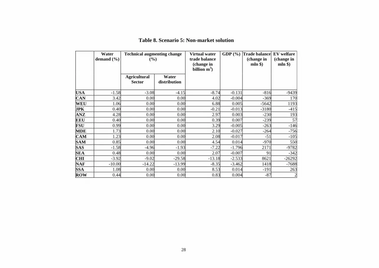
Table 8. Scenario 5: Non-market solution

Water

demand (%)

Technical augmenting change (%)

Virtual water trade balance

(change in billion m3)

GDP (%) Trade balance (change in

mln $)

EV welfare (change in

mln $)

Agricultural Sector

Water distribution

USA -1.58 -3.08 -4.15 -8.74 -0.131 -816 -9439CAN 3.42 0.00 0.00 4.02 -0.004 -369 170WEU 1.06 0.00 0.00 6.88 0.005 -5642 1193JPK 0.40 0.00 0.00 -0.21 -0.013 -3180 -415ANZ 4.28 0.00 0.00 2.97 0.003 -230 193EEU 0.40 0.00 0.00 0.39 0.007 -239 57FSU 0.99 0.00 0.00 3.29 -0.005 -263 -146MDE 1.73 0.00 0.00 2.10 -0.027 -264 -756CAM 1.23 0.00 0.00 2.08 -0.017 -51 -105SAM 0.85 0.00 0.00 4.54 0.014 -970 550SAS -1.58 -4.96 -1.93 -7.22 -1.796 2171 -9782SEA 0.48 0.00 0.00 2.07 -0.007 91 -342CHI -3.92 -9.02 -29.58 -13.18 -2.533 8621 -26292NAF -10.00 -14.22 -13.99 -8.35 -3.462 1418 -7688SSA 1.08 0.00 0.00 8.53 0.014 -191 263ROW 0.44 0.00 0.00 0.83 0.004 -87 2

28