Embed Size (px)
Citation preview

Centerfor
Economic Research
No. 2000-69
THE ECONOMICS OF SHALLOW LAKES
By Karl-Göran Mäler, Anastasios Xepapadeas and Aart de Zeeuw
August 2000
ISSN 0924-7815

This research was initiated at a meeting of the Resilience Network which had financial support from the1
MacArthur Foundation. We are very grateful for the advice and comments of (in alphabetical order) WilliamBrock, Steve Carpenter, Davis Dechert, Marten Scheffer, Perry Shapiro, Sjak Smulders, Robert Solow, DavidStarrett and Florian Wagener.
Mailing address: P.O. Box 90153, 5000 LE Tilburg, the Netherlands; e-mail: [email protected]
1
The Economics of Shallow Lakes1
Karl-Göran Mäler
The Beijer International Institute of Ecological Economics
Anastasios Xepapadeas
Department of Economics, University of Crete
Aart de Zeeuw
Department of Economics and CentER, Tilburg University2
Abstract
Ecological systems such as shallow lakes are usually non-linear and display discontinuities and
hysteresis in their behaviour. These systems often also provide conflicting services as a resource and
a waste sink. This implies that the economic analysis of these systems requires to solve a non-
standard optimal control problem or, in case of a common property resource, a non-standard
differential game. This paper provides the optimal management solution and the open-loop Nash
equilibrium for a dynamic economic analysis of the model for a shallow lake. It also investigates
whether it is possible to induce optimal management in case of common use of the lake, by means
of a tax. Furthermore, an interesting property for the feedback Nash equilibrium is derived.
Key words: non-linear differential games, ecological systems.
JEL-codes: 020, 720.

2
1. Introduction
The purpose of this paper is to develop an economic analysis of the shallow lake. Lakes have been
studied intensively and the shallow lake model is well tested and documented, so that the analysis
has a direct meaning. However, the lake model can also be viewed as a metaphor for many of the
ecological problems facing mankind today, so that the analysis developed in this paper will have a
wider applicability. The economic analysis is especially challenging because of the non-linear
dynamics of the lake (which yields non-convex decision problems) and the gaming aspects related
to the common property character of the lake.
It has been observed that shallow lakes, due to a heavy use of fertilizers on surrounding land and
an increased inflow of waste water from human settlements and industries, at some point tend to
flip from a clear state to a turbid state with a greenish look caused by a dominance of
phytoplankton (Carpenter and Cottingham, 1997; Scheffer, 1997). The release of nutrients,
especially phosphorus, into the lake stimulates the growth of phytoplankton and in addition to that,
the resulting turbidity prevents light to reach the bottom of the lake so that submerged vegetation
disappears. With the vegetation many species disappear such as waterfleas which graze on
phytoplankton. It has also been observed that shallow lakes are hard to restore in the sense that the
nutrient loads have to be reduced below the level where the flip occurred before the lake flips back
to a clear state. The positive feedback through the effect on the submerged vegetation is one
explanation for this so-called hysteresis effect.
Ecological systems often display discontinuities in the equilibrium states of the system over time.
A seminal paper in this area models the sudden outbreak of an insect, called the spruce budworm,
and the long time it takes before the budworm density jumps back to a low number again (Ludwig,
Jones and Holling, 1978). Technically, this hysteresis effect can be modelled by a non-linear
differential equation which has multiple equilibria with separated domains of attraction in a certain
range of the exogenous variable. Other examples of ecological systems with hysteresis are described
in Ludwig, Walker and Holling (1997).
In the ecological literature, management of shallow lakes is mostly interpreted as preventing the lake
to flip or, if it flips, as restoring the lake in its original state. However, this approach denies the

3
economics of the problem in the sense of the trade-offs between the utility of the agricultural
activities, which are responsible for the release of phosphorus, and the utility of a clear lake. When
the lake flips to a green turbid state, the value of the ecological services of the lake (e.g. the intake
of water and recreation) decreases but this situation corresponds to a high level of agricultural
activities. It depends, of course, on the relative weight attached to these welfare components
whether it is better to keep the lake clear or not. Note that if it is better to keep the lake clear, it is
very costly to let the lake flip first because of the hysteresis. A second economic issue is that lakes
are usually common property resources and therefore suffer from sub-optimal use, in the absence
of coordination.
In the first part of the paper, very simple welfare analysis is done on the possible equilibria of the
lake model. Relative weights are chosen such that it is optimal to manage the lake in one of its clear
states, called oligotrophic states. It is shown, however, that when the lake is shared by more than
one community, two Nash equilibria occur: one in an oligotrophic state and one in a dirty state,
called a eutrophic state. In the second part of the paper, intertemporal welfare is maximized subject
to the dynamics of the lake. It is shown that in case the discount rate is low enough, an optimal
path for phosphorus loadings exists, from each initial condition of the lake, which moves the lake
towards its optimal steady-state. When the lake is shared by more than one community, a non-linear
differential game has to be solved. The phase-diagram for the open-loop Nash equilibrium has three
steady-states, two of which are saddle-point stable and correspond to the Nash equilibria found in
the first part of the paper. The third point is unstable and displays complex dynamics. However,
it is shown that a so-called Skiba point exists which splits the possible initial conditions of the lake
in an area from where the Nash equilibrium loading trajectory will approach the oligotrophic saddle-
point, and an area from where the eutrophic saddle-point results.
The question arises whether it is possible, by levying a tax on the loading of phosphorus, to induce
the communities to follow an optimal management path. Note that if the communities are locked
in the eutrophic Nash equilibrium, a straight path to the optimal steady-state is not feasible due to
the hysteresis. Assuming that it is not possible to implement a time-varying tax, the answer depends
on the number of communities. It is shown that if the number is low enough, a constant tax yields
a Nash equilibrium path that moves towards the optimal steady-state (although this path will not
be the same as the optimal management path, of course). If the number is high, however, more
saddle-points arise again and the dynamics becomes very complex, so that there is no guarantee that

ÿP(t) ' L(t)& sP(t)% r P 2(t)
P 2(t)%m 2, P(0)'P0,
ÿx(t) ' a(t)&bx(t)% x 2(t)
x 2(t)%1, x(0)'x0.
4
(1)
(2)
a constant tax can induce optimal management of the lake in the long run.
A final issue regards the type of Nash equilibrium employed in the analysis. It is well-known that
the open-loop Nash equilibrium is not strongly time-consistent and therefore a feedback Nash
equilibrium is preferred. However, due to the non-linear dynamics of the lake, it is very difficult to
find a feedback Nash equilibrium. In the last section of the paper, an interesting property of the
equilibrium is derived, in case it exists and under certain conditions, but it is left for further research
to try to identify this equilibrium.
The paper is organized as follows. Section 2 describes the shallow lake model. Section 3 is
concerned with the economics of the lake equilibria and section 4 with the dynamic welfare analysis
of the lake. Section 4 contains the case of optimal management, the open-loop Nash equilibrium,
the effect of taxes and the feedback Nash equilibrium. Section 5 concludes the paper.
2. The Lake Model
Shallow lakes have been studied intensively over the last two decades and it has been shown that
the essential dynamics of the eutrophication process can be modelled by the differential equation
where P is the amount of phosphorus in algae, L is the input of phosphorus (the “loading”), s is
the rate of loss consisting of sedimentation, outflow and sequestration in other biomass, r is the
maximum rate of internal loading and m is the anoxic level (see for an extensive treatment of the
lake model Carpenter and Cottingham (1997) or Scheffer (1997)). Less is known about deep lakes
but from what is known now, it can be expected that the same type of model will be adequate.
However, estimates of the parameters of this differential equation for different lakes vary
considerably, so that a wide range of possible values has to be considered.
By substituting x = P/m, a = L/r, b = sm/r and by changing the time scale to rt/m, equation (1) can
be rewritten as

5
In order to understand some of the important features of this model, suppose that the loading a
is constant. For high values of a, differential equation (2) has one stable equilibrium. For low values
of a, three situations can occur, depending on the value of the parameter b. If b $ 3%3/8, all values
of a lead to one stable equilibrium (see figure 1). If b # ½, low values of a yield two equilibria for
the differential equation (2). The third root of the right-hand side of equation (2) determines the
domains of attraction: above this point, the high equilibrium will result and below this point the low
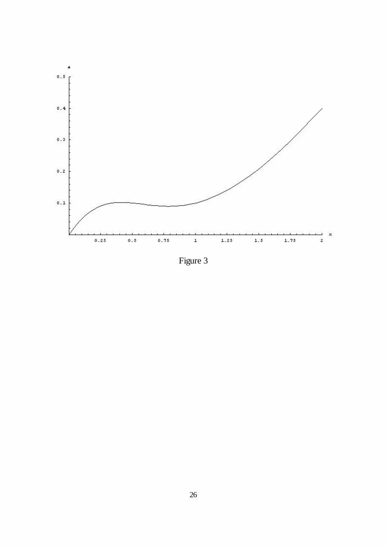
equilibrium (see figure 2). If ½ < b < 3%3/8, low values of a first yield one stable equilibrium again,
followed by a range of a’s with two equilibria (see figure 3).
It is easy to see a hysteresis effect now for b < 3%3/8. If the loading a is gradually increased, at first
the equilibrium level of phosphorus remains low: the lake remains in an oligotrophic state with a
high level of ecological services. At a certain point, however, the lake flips to a high equilibrium level
of phosphorus. To put it differently, the lake flips to a eutrophic state with a low level of ecological
services. If it is then decided to lower the loading a in order to try to bring the lake back to an
oligotrophic state, it is not enough to reduce a just below that flip-point. If b is high enough (½ <
b < 3%3/8, figure 3), it can still be done, but a has to be reduced further until the lake flips back to
an oligotrophic state. If b # ½ (figure 2), however, then the lake is trapped in high equilibrium levels
of phosphorus which means that the first flip is irreversible. In that case, only a change in the
parameter b (e.g., by releasing a certain type of fish and thus changing the fauna) can restore the
lake. In the sequel of the paper, it is assumed that the parameter b = 0.6 so that the lake displays
hysteresis but a flip to a eutrophic state is reversible. Furthermore, the loading a will not be
exogenous anymore but subject to control. In section 3, a is still constant and the trade-off is
considered between the benefits of being able to release that constant amount of phosphorus, on
the one hand, and the resulting damage to the lake, on the other hand. Section 4 provides a full
dynamic analysis where a can change over time.
[Insert figures 1, 2, 3 about here]
3. Economic Analysis of the Lake Equilibria
Several interest groups operate in relation with the lake, modelled in section 2. Because the release
of phosphorus into the lake is due to agricultural activity, at least the farmers have an interest in
being able to increase the loading. In that way, the agricultural sector can grow without the need

maximize jn
i'1lnai&ncx 2 s.t. a&bx% x 2
x 2%1' 0, a'j
n
i'1ai.
b& 2x
(x 2%1)2&2cx(bx& x 2
x 2%1) ' 0.
6
(3)
(4)
to invest in new technology in order to decrease the emission-output ratio. On the other hand, a
clean lake is preferred by fishermen, drinking water companies, other industry that makes use of
the water, and people who spend leisure time on or along the lake. Suppose a community or
country, balancing these different interests, can agree on a welfare function of the form ln a - cx ,2
c > 0. The lake has value as a waste sink for agriculture (ln a) and it provides ecological services that
decrease with the amount of phosphorus (-cx ). The parameter c reflects the relative weight of these2
welfare components. Suppose, furthermore, that the lake is shared by n communities or countries
with the same welfare function. In this section it is assumed that the communities choose constant
loading levels a , i = 1,...,n, and that the amount of phosphorus adjusts instantaneously to itsi
equilibrium level. A logarithmic functional form is used, because then the optimal management
outcome has the invariance property in the sense that it is independent of the number of
communities and does not change when this number is varied. It is assumed that the area around
the lake is large enough so that adding new communities does not lead to crowding out, and it is
assumed that the objectives are additive in the number n.
Optimal management of the lake requires to solve
Simple calculus shows that the optimal amount of phosphorus is determined by
Optimal management, of course, does not necessarily yield an oligotrophic state for the lake. If the
communities attach a relatively low weight c to ecological services, it can be optimal to choose a
eutrophic state with a high level of agricultural activities. It is easy to show that for large values of
c, the optimal management problem has one maximum for an x below the flip-point. As the value
of c is decreased, first a local maximum appears for a high x whereas the global maximum is still
achieved for a low x, but for c low enough (i.e. c # 0.36) the global maximum occurs for a high x
beyond the flip-point. In the sequel of the paper it is assumed that enough weight (i.e. c = 1) is
attached to the services of the lake to make it optimal to aim for an oligotrophic state.
If c = 1, equation (4) yields x* = 0.33 with total loading a* = 0.1. Note that the same level of total

maximize lnai& cx 2, i'1,...,n, s.t. a&bx% x 2
x 2%1' 0, a'j
n
i'1ai.
b& 2x
(x 2%1)2&2
cn
x(bx& x 2
x 2%1) ' 0.
7
(5)
(6)
loading can also lead to the eutrophic state x = 1, if the initial amount of phosphorus is in the upper
domain of attraction (see figure 3). A flip occurs when total loading is increased to a = 0.1021, so
that the lake is managed not far from what is called the “edge of hysteresis” (Brock, Carpenter and
Ludwig, 1997). A small mistake may cause a flip with high costs, not only directly because of a jump
to a high x but also indirectly because of the long return path.
If the communities do not cooperate in managing the lake, it is assumed a Nash equilibrium results
which requires to solve
Simple calculus shows that the Nash equilibrium level of phosphorus is determined by
If c = 1 again and if the number of communities n = 2, equation (6) has three solutions, two of
which correspond to a Nash equilibrium. The first Nash equilibrium yields x = 0.36 with totalN1
loading a = 0.1012. The lake is still in an oligotrophic state but closer to the edge of hysteresis.N1
However, the second Nash equilibrium yields an eutrophic state x = 1.51 with total loading aN N2 2
= 0.2108. Welfare under optimal management and in the oligotrophic Nash equilibrium are
comparable, but welfare in the eutrophic Nash equilibrium is much lower. Moreover, when the
communities are locked into the second Nash equilibrium and decide to coordinate, it is much more
difficult to reach the optimal management outcome, due to the hysteresis. It is not enough to
reduce total loading to 0.1. It has to be reduced to 0.0898 first, in order to flip back to an
oligotrophic state, and can then be increased to 0.1 again.
If n > 2, these numbers change of course, but it is easy to see that for all b in the range with
hysteresis and reversibility (½ < b < 3%3/8), on which this paper focuses, always two Nash
equilibria occur. In fact, equation (6) intersects the curve for the lake equilibria with the curve
described by (n/2cx)(b - 2x/(x + 1) ). For b in the range given above, this curve has a negative part2 2
for x in a positive range. Furthermore, it approaches infinity for x 9 0 and it approaches zero from
above for x 6 4. Increasing the number of communities n implies that the curve is stretched out
but the three intersection points remain, two of which are Nash equilibria.

Wi ' m4
0
e &ñt [lnai(t)& cx 2(t)]dt, i'1,...,n,
1ai(t)
%ë(t) ' 0, i'1,...,n,
ÿë(t) ' [(b%ñ)&2x(t)
(x 2(t)%1)2]ë(t)%2ncx(t),
ÿa(t) ' &[(b%ñ)&2x(t)
(x 2(t)%1)2]a(t)%2cx(t)a 2(t).
8
(7)
(8)
(9)
(10)
In the next section the loading a can change over time and the amount of phosphorus does not
adjust instantaneously to its equilibrium level but gradually according to equation (2), which turns
the optimal management problem into an optimal control problem and the static game into a
differential game. The Nash solutions found in this section return (approximately) as saddle-point
stable steady-states with solution trajectories that may have to bend around the flip-point.
4. Dynamic Economic Analysis of the Lake Model
Suppose that the problem has an infinite horizon, so that the objectives become
where ñ > 0 is the discount rate.
4.1 Optimal management
Optimal management requires to maximize the sum of the objectives W , subject to equation (2)i
with a = Óa . This is an optimal control problem and the maximum principle yields the necessaryi
conditions
with a transversality condition on the co-state ë , and equation (2). Substitution of (8) into (9),
symmetry and multiplication by n yields

1ai(t)
%ëi(t) ' 0, i'1,...,n,
9
(11)
The solution is given by the set of differential equations (2) and (10), and the transversality
condition. Note that b = 0.6 (see section 2) and c = 1 (see section 3). The phase-diagram in the (x,
a)-plane is drawn in figure 4a. One curve represents the steady-states for x and can be recognized
as the lake equilibria, which were discussed in sections 2 and 3. The other curve represents the
steady-states for a. Its position depends on the discount rate ñ. If the discount rate is low enough
(ñ < 0.1), this curve intersects the first curve only once in a point that is saddle-point stable. If the
discount rate is higher, the second curve moves up, it intersects the first curve three times, and the
analysis becomes similar to the analysis of the open-loop Nash equilibrium below. It is assumed
here that the discount rate ñ = 0.03, which yields the graph in figure 4a. The steady-state is close
to the static optimal management solution in section 3, and converges to that point when the
discount rate goes to 0. The optimal solution prescribes to jump, at any initial state of the lake, to
the stable manifold and to move towards the steady-state. Given the non-linearity of the problem,
it is not easy to obtain an analytical expression for the stable manifold but a numerical
approximation is not difficult to develop. Starting at the steady-state point, the characteristic vector
corresponding to the negative eigenvalue of the Jacobian matrix determines the direction of the
stable manifold. Working backwards from the steady-state in small steps, a piecewise linear
approximation of the stable manifold is then found and the approximation gets better the smaller
the steps. With Mathematica (Wolfram, 1999), the stable and unstable manifolds for the set of
differential equations (2) and (10) can be drawn (see figure 4b). Note that the stable manifold can
be reached from all initial states x and bends around the lower flip-point (see also section 3).0
[Insert figures 4a, 4b about here]
4.2 Open-loop Nash equilibrium
The open-loop Nash equilibrium (Bas,ar and Olsder, 1982) is found by applying the maximum
principle to each objective W , i = 1,...,n, separately (fixing a for j … i) subject to equation (2) withi j
a = Óa . The set of necessary conditions becomesi

ë ÿi(t) ' [(b%ñ)&2x(t)
(x 2(t)%1)2]ëi(t)%2cx(t), i'1,...,n,
ÿa(t) ' &[(b%ñ)&2x(t)
(x 2(t)%1)2]a(t)%2
cn
x(t)a 2(t).
10
(12)
(13)
with transversality conditions on the co-states ë , and equation (2). Substitution of (11) into (12),i
symmetry and multiplication by n yields
The open-loop Nash equilibrium is given by the set of differential equations (2) and (13), and the
transversality conditions. The phase-diagram for two communities n = 2 (and b = 0.6, c = 1, ñ =
0.03) in the (x, a)-plane is drawn in figure 5a. The steady-state curves for x and a now have three
intersection points. The intersection points on the left and on the right are saddle-point stable and
yield possible steady-states for the Nash equilibrium in an oligotrophic and in a eutrophic area,
respectively. The intersection point in the middle is unstable with complex eigenvalues. Again with
Mathematica (Wolfram, 1999), the stable and unstable manifolds for the set of differential equations
(2) and (13) can be drawn (see figure 5b). The trajectories of the stable manifold curl a while from
the intersection point in the middle and then go either to the steady-state on the left or to the
steady-state on the right. It is clear that when the initial state x lies to the right of the set of curls,0
the open-loop Nash equilibrium follows the upper trajectory to the steady-state on the right, and
when the initial state lies to the left of that area, it follows the lower trajectory to the steady-state
on the left. However, it is more difficult to see what happens in the range in between. It can be
shown (Appendix A) that a state x exists such that for x < x , the open-loop Nash equilibriumS 0 S
jumps to the lower trajectory and moves towards the oligotrophic steady-state whereas for x > x ,0 S
it jumps to the upper trajectory and moves towards the eutrophic steady-state. The point x is calledS
a Skiba point because it was introduced by Skiba in an optimal growth model with a convex-
concave production function (Skiba, 1978, Brock and Malliaris, 1989).
[Insert figures 5a, 5b about here]
If n > 2, the same arguments as in section 3 can be used to show that always two open-loop Nash
equilibria occur. Note, however, by inspection of equation (13), that the arguments do not hold for
all b in the range (½, 3%3/8) anymore, because of the positive discount rate ñ, but only for b + ñ <
3%3/8, which holds for the specific values chosen for b and ñ.

Wi ' m4
0
e &ñt [lnai(t)&ô(t)ai(t)& cx 2(t)] dt, i'1,...,n.
1ai(t)
&ô(t)%ëi(t) ' 0, i'1,...,n.
11
(14)
(15)
Before turning to the question whether a tax can induce the communities to choose loadings
according to the optimal management trajectory, it is useful to make a few general remarks on the
analysis above. First, when comparing equations (10) and (13), it is immediately clear that the open-
loop Nash equilibrium also results under optimal management with parameter c/n instead of c. It
is an example of a potential game where a Nash equilibrium results when some constructed
objective is maximized (Monderer and Shapley, 1996; Dechert and Brock, 1999). Second, it also
means that all outcomes (optimal management with varying relative weight c, and symmetric open-
loop Nash equilibria with fixed c but varying number of communities n) can be traced by solving
an optimal control problem leading to a set of differential equations with parameter c/n. This
parameter can be denoted as a bifurcation parameter and it can be shown that only saddle-node and
heteroclinic bifurcations can occur (Wagener, 1999; Brock and Starrett, 1999). Third, similar
dynamics is found in models for external economies with multiple equilibria but in these models
the solution is not driven by maximizing an objective but by self-fulfilling expectations. The idea
in these models is to show that outside the curls, only history (initial conditions) determines which
equilibrium is reached but in the range with curls, expectations play a role (Krugman, 1991;
Matsuyama, 1991). In this paper, however, an objective is maximized which yields a Skiba point, so
that only initial conditions determine the outcome both for optimal management and the symmetric
open-loop Nash equilibrium.
4.3 Taxes
Consider the case of achieving the unique steady-state amount of phosphorus under optimal
management by a tax ô on phosphorus loading. Under the tax scheme the objectives (7) of the
open-loop differential game change to
The maximum principle requires for the optimal choice of phosphorus loading at each point in time
that

ô( ' &(n&1)ë(
n'
(n&1)
a (,
ÿa(t) ' &[(b%ñ)&2x(t)
(x 2(t)%1)2][a(t)& ô(
na 2(t)]%2
cn
x(t)a 2(t)
12
(16)
(17)
In order to obtain the loading that corresponds to optimal management, it is immediately clear by
comparing (8) to (15) that the tax on loading should be chosen such that ô(t) = -ë (t) + ë (t). Thisi
implies that the tax bridges the gap between the social shadow cost of the accumulated phosphorus
ë (t) and the private shadow cost of the accumulated phosphorus ë (t) that causes the steady-statei
phosphorus levels in the open-loop Nash equilibrium to exceed the (unique) steady-state
phosphorus level under optimal management. The tax rate will, however, be time dependent, since
it has to equalize cooperative and non-cooperative loading at every point in time. Although optimal,
such a tax will be very difficult to implement, since it would require a regulating institution to
continuously change the tax rate. Another, more realistic, approach would be to choose a fixed tax
rate on loading, defined such that the non-cooperative steady-state phosphorus level under the
constant tax equals the steady-state phosphorus level under optimal management. This tax will be
called the optimal steady-state tax (OSST).
By comparing (9) to (16) and using (10), it is easy to see that the OSST ô* is given by
where ë * is the value of the co-state and a* is total loading in the steady-state under optimal
management. Under this constant tax scheme, the open-loop Nash equilibrium will be given by the
set of differential equations (2) and, instead of (13),
with a transversality condition.
It is easy to check that the steady-state (x*, a*) for the set of differential equations (2) and (10)
under optimal management is also a steady-state for the set of differential equations (2) and (17) in
the open-loop Nash equilibrium under the constant tax ô*. By substituting a(t) = a* and ô* = (n -
1)/a* in the second term between brackets of the right-hand side of equation (17), this term reduces
to a*/n. It is then easy to see that (x*, a*) is also a point on the curve representing the steady-states
for total loading a in the open-loop Nash equilibrium under the OSST. However, the rest of this
curve differs from the one under optimal management.
It should be made clear that the OSST leads to the optimal management steady-state but the path
under the OSST that determines the transition to the steady-state is not the same as the optimal

a '
(b%ñ)&2x
(x 2%1)2
2cn
x% [(b%ñ)&2x
(x 2%1)2](n&1)
na (
.
2cx(n&1)
% [(b%ñ)&2x
(x 2%1)2]
1
a (' 0.
13
(18)
(19)
management path. Coincidence of the optimal management path and the regulated path requires
to use the time-dependent tax. To put it differently, the stable manifold of the optimal management
problem is not the same as the stable manifold of the regulated problem, although both approach
the same saddle-point.
If the number of communities n = 2, the phase-diagram under the OSST in the (x, a)-plane is
drawn in figure 6a. Although this figure differs from figure 4a for optimal management, it is
qualitatively the same. It has one saddle-point and a corresponding stable manifold. Starting at both
unregulated Nash equilibrium steady-states, the two communities will change their loadings under
the OSST and the equilibrium path will follow this stable manifold and move towards the optimal
management steady-state. Starting at the oligotrophic Nash equilibrium, this is a short trajectory,
but starting at the eutrophic Nash equilibrium, the path has to bend around the flip-point.
[Insert figures 6a, 6b, 6c about here]
Increasing the number of communities n, at a certain point the phase-diagram under the OSST
becomes very complicated. From equation (17), the curve representing the steady-states for a is
given by
The denominator of the right-hand side of equation (18) is zero if and only if
For n = 2 the left-hand side of equation (19) is positive, but for n > 7 equation (19) has two roots
which yield two vertical asymptotes for the curve given by equation (18). Note that this
phenomenon occurs because the term between brackets is partly negative which is caused by the
specific choice of b and ñ (see also section 4.2). Moreover, if n goes to infinity, the curve approaches
a = a*, but this convergence is not uniform, due to the two discontinuities. An example of such a
phase-diagram under the OSST is drawn in figure 6b where n = 10. This case still has only one

ë ÿi(t) ' [(b%ñ)&2x(t)
(x 2(t)%1)2&j
n
j…ih )
j (x(t))]ëi(t)%2cx(t), i'1,...,n,
ÿa(t) ' &[(b%ñ)&2x(t)
(x 2(t)%1)2& (n&1)h )(x(t))]a(t)%2
cn
x(t)a 2(t),
14
(20)
(21)
saddle-point stable steady-state. If n gets large, it is to be expected that the curve has more
intersection points with the curve representing the lake equilibria, because of the convergence to
a*. This implies the possibility that multiple steady-states occur under the OSST. An example is
drawn in figure 6c where n = 100. This case has three steady-states again, two of which are saddle-
point stable, whereas the middle one is unstable. For a lower discount rate ñ and a higher number
of communities n, it may happen that two more steady-states occur between the asymptotes, one
unstable and one saddle-point. The existence of a second steady-state characterized by saddle-point
stability leads to the conclusion that if the number of communities n is high, the optimal steady-
state tax may not work. Depending on the initial conditions, the OSST may direct the equilibrium
path towards a steady-state with a higher phosphorus level than in the optimal management steady-
state.
4.4 Feedback Nash equilibrium
The open-loop Nash equilibrium is weakly time-consistent but not strongly time-consistent which
implies that the equilibrium is not robust against unexpected changes in the state of the lake (Bas,ar,
1989). To obtain an equilibrium with the Markov perfect property, the feedback Nash equilibrium
has to be found which means that the Hamilton-Jacobi-Bellman equation for the game has to be
solved. This is a very difficult problem because it is not clear what the value function will look like
due to the non-linearity of the lake model. However, assuming that a symmetric feedback Nash
equilibrium exists, it is possible to consider the properties, which is the topic of this section.
Suppose that the loading strategies in the feedback Nash equilibrium are given by a = h (x), i = 1,..,n.i i
The maximum principle then yields, instead of equation (12),
and, instead of equation (13),
where h denotes the symmetric feedback Nash equilibrium loading strategy and h’ denotes the

ñV(x) ' max [lnai& cx 2%Vx(x)[ai% (n&1)h(x)&bx% x 2
x 2%1]],
1ai
' &Vx(x) Y ai :' h(x) '&1
Vx(x)Y h )(x) '
Vxx(x)
V 2x (x)
.
15
(22)
(23)
derivative of h with respect to the state x of the lake.
It can be seen from (21) that if h’(x) < 0, the steady-state curve for a in figure 5a moves up so that
the intersection points with the steady-state curve for x move to the right. It follows that the
steady-state amount of phosphorus and total loadings will be higher in the feedback Nash
equilibrium than in the open-loop Nash equilibrium. This would confirm the intuition derived in
similar type of problems (van der Ploeg and de Zeeuw, 1992). If a community knows that the other
communities will respond to a higher amount of phosphorus in the lake with lower loadings, it can
load more at the margin because the extra loading will be partly offset by the reactions of the other
communities. Since all communities argue in this way, total loading in equilibrium is higher than in
the case the loadings are not conditioned on the state of the lake as in the open-loop Nash
equilibrium.
The question is whether it can be shown that h’(x) < 0. It is very difficult to explicitly solve for h(x)
but by exploiting the first-order condition of maximization in the Hamilton-Jacobi-Bellman
equation, a relation can be established with concavity of the value function.
The HJB-equation for community i, i = 1,..,n, is given by
where V denotes the value function. The first-order condition yields
It follows that the feedback Nash equilibrium strategy h has a negative slope in the region of
concavity of the value function. In Appendix B it is shown that, under certain conditions, the value
function is concave in the oligotrophic region. This would then imply that if a feedback Nash
equilibrium exists below the flip-point, it must lead to a higher steady-state amount of phosphorus,
with higher total loadings, than the open-loop Nash equilibrium.
5. Conclusion

16
Economics of ecological systems is a much neglected area in the literature. Furthermore, non-
linearities in the dynamics of these systems and the common property aspect of the function as a
resource and a waste sink, present interesting challenges to economic theory. This paper focuses
on the shallow lake as an example, but also because much is known about shallow lakes in the
ecological literature. However, the analysis applies to all models that are driven by convex-concave
relations, and models with this feature are very typical for mathematical models in ecology (see
Murray, 1989).
Internal loading of phosphorus in shallow lakes causes the lake model to be non-linear. As a
consequence, even in the case that optimal management of the lake has only one steady-state with
saddle-point stability, either an increase in the discount rate or an increase in the number of
communities, sharing the lake, leads to more saddle-points and complicated dynamics in between.
However, a Skiba point exists, which means that in these cases the initial level of accumulated
phosphorus determines whether the lake will end up in a clear or a turbid state. For a small number
of communities, a constant tax on the loading of phosphorus can induce optimal behaviour and
a return to a clear state, but for a large number this may not work. The analysis employs the open-
loop Nash equilibrium to characterize non-cooperative behaviour. The feedback Nash equilibrium
would be more appropriate but is very difficult to identify for this problem. It is shown, however,
that it is to be expected that this equilibrium will result in even higher equilibrium amounts of
phosphorus.
References
Bas,ar, T. and G.J. Olsder (1982), Dynamic Noncooperative Game Theory, Academic Press, New York.
Bas,ar, T. (1989), Time consistency and robustness on equilibria in noncooperative dynamic games,
in F. van der Ploeg and A.J. de Zeeuw (eds.), Dynamic Policy Games in Economics, Contributions to
Economic Analysis 181, North Holland, Amsterdam, 9-54.
Brock, W.A., S.R. Carpenter and D. Ludwig (1997), Notes on optimal management of a lake subject
to flips, Working Paper, University of Wisconsin.
Brock, W.A. and D. Starrett (1999), Nonconvexities in ecological management problems, Working

17
Paper, University of Wisconsin.
Brock, W.A. and A.G. Malliaris (1989), Differential Equations, Stability and Chaos in Dynamic Economics,
North Holland, Amsterdam.
Carpenter, S.R. and K.L. Cottingham (1997), Resilience and restoration of lakes, Conservation Ecology
1:2.
Crandall, M.G., H. Ishii and P.-L. Lions (1992), User’s guide to viscosity solutions of second order
partial differential equations, Bulletin of the American Mathematical Society 27, 1-25.
Dechert, W.D. and W.A. Brock (1999), Lakegame, Working Paper, University of Houston.
Krugman, P. (1991), History versus expectations, Quarterly Journal of Economics, CVI, 651-667.
Ludwig, D., D.D. Jones and C.S. Holling (1978), Qualitative analysis of insect outbreak systems: the
spruce budworm and forest, Journal of Animal Ecology 47, 315-332.
Ludwig, D., B.H. Walker and C.S. Holling (1997), Sustainability, stability and resilience, Conservation
Ecology 1:7.
Matsuyama, K. (1991), Increasing returns, industrialization, and indeterminacy of equilibrium,
Quarterly Journal of Economics CVI, 617-650.
Monderer, D. and L.S. Shapley (1996), Potential games, Games and Economic Behaviour 14, 124-143.
Murray, J.D. (1989), Mathematical Biology, Springer Verlag, Berlin.
van der Ploeg, F. and A.J. de Zeeuw (1992), International aspects of pollution control, Environmental
& Resource Economics 2, 117-139.
Scheffer, M. (1997), Ecology of Shallow Lakes, Chapman and Hall, New York.

W ' m4
0
e &ñt [jn
i'1lnai(t)& cx 2(t)]dt.
H ' e &ñtg(x,a1,..,an)%µf(x,a1,..,an),
g(x,a1,..,an) ' jn
i'1lnai& cx 2, f(x,a1,..,an) ' j
n
i'1ai&bx%
x 2
x 2%1,
H̃ ' g(x,a1,..,an)%ëf(x,a1,..,an), ë' e ñtµ.
18
(A1)
(A2)
(A3)
(A4)
Skiba, A.K. (1978), Optimal growth with a convex-concave production function, Econometrica 46,
3, 527-539.
Wagener, F.O.O. (1999), Shallow lakes, Working Paper, University of Amsterdam.
Wolfram, S. (1999), The Mathematica Book, 4 ed., Wolfram Media / Cambridge University Press,th
Cambridge.
Appendix A: The Skiba point
As also noted later in the main text, the open-loop Nash equilibrium results from maximizing the
welfare objective (a potential function)
What follows is strongly based on Wagener (1999).
Define the Hamiltonian function
where
and define the current value Hamiltonian function
The maximum principle yields the necessary conditions (8), (9) and (2) with the parameter c
replaced by c/n, which then yields the set of differential equations (2) and (13) for the open-loop
Nash equilibrium with the phase-diagram given in figure 5a and the stable and unstable manifolds
in figure 5b.

dHdt
'MHMx
dxdt%MHMµ
dµdt%MHMt
'MHMx
MHMµ
&MHMµ
MHMx
%MHMt
' &ñe &ñtg.
H̃(0) ' H(0) ' &m4
0
dHdt
dt ' m4
0
ñe &ñtg dt ' ñW.
dWdx
'dWdt
dtdx
'1ñ
dH̃dt
1f'
1ñ
[MH̃Mx
f% f (ñë&MH̃Mx
]1f' ë.
ë ' &1ai
, i'1,..,n, Y ë ' &na
(a'jn
i'1ai).
mdWdx
dx ' më dx ' m&na
dx < 0.
19
(A5)
(A6)
(A7)
(A8)
(A9)
Denote the x-coordinate of the oligotrophic steady-state as x and of the eutrophic steady-state as1
x , and denote the range with curls as [x , x ], where x and x are the x-coordinates of the4 2 3 2 3
intersection points of the outer upper curl and the outer lower curl with the curve representing the
steady-states for x (f = 0), respectively.
Along trajectories, it holds that
It follows that
Furthermore,
Condition (8) yields
The proof of the existence of a unique Skiba point takes four steps.
1) Suppose the initial condition x is in the interior of the range [x , x ].0 2 3
It is better to jump immediately to the upper trajectory instead of to the same trajectory some point
earlier, or to the lower trajectory instead of to the same trajectory some point earlier, because the
welfare difference
2) Suppose the initial condition is x . The choice is either to jump to the upper trajectory and start2
at the intersection point with f = 0 or to jump to the lower trajectory, by a proper choice of intial
loadings a. Because

MWMa
'1ñMH̃Ma
'1ñj
n
i'1
MMai
(g%ëf) '1ñj
n
i'1
1
a 2i
f ' 1ñ
n 3
a 2f
ÄW(x2) < 0, ÄW(x3) > 0,ddx
ÄW ' ë2&ë1 > 0.
ÄW(xS) ' 0; ÄW(x) < 0, x0 [x2,xS); ÄW(x) > 0, x0 (xS,x3].
V(ëx )
0 % (1&ë)x ))
0 ) $ ëV(x )
0)% (1&ë)V(x ))
0 ).
20
(A10)
(A11)
(A12)
(B1)
and f < 0 below the intersection point, the welfare difference between the upper trajectory and the
lower trajectory is negative, so that it is better to jump to the lower trajectory at x .2
3) Suppose the initial condition is x . The choice is either to jump to the lower trajectory and start3
at the intersection point with f = 0 or to jump to the upper trajectory. Because above the
intersection point f > 0, it follows from equation (A10) that the welfare difference between the
upper trajectory and the lower trajectory is positive, so that it is better to jump to the upper
trajectory at x .3
4) Compare now the upper trajectory leading to steady-state on the right, with co-state ë , and the2
lower trajectory leading to the steady-state on the left, with co-state ë . Denote the welfare1
difference as ÄW. Using the results in steps 2-3 and equations (A7)-(A8), it follows that
From (A11) it follows that a point x in the interior of the range [x , x ] exists, such thatS 2 3
The point x is called a Skiba point and (A12) implies that if the initial amount of phosphorus xS 0
is on the left-hand side of the Skiba point, the equilibrium jumps to the lower trajectory and moves
towards the steady-state on the left and if the initial amount of phosphorus x is on the right-hand0
side of the Skiba point, the equilibrium jumps to the upper trajectory and moves towards the
steady-state on the right.
Appendix B: Concavity of the value function
The value function V(x) is concave if for any two initial states x' and x" of the lake and for all ë 00 0
[0,1], it holds that

ëWi(h(x )),x ))% (1&ë)Wi(h(x ))),x ))) # Wi(ëh(x ))% (1&ë)h(x ))), ëx )% (1&ë)x ))),
Wi(h(x̂), x̂) $ Wi(ëh(x ))% (1&ë)h(x ))), y),
ÿx ' ëh(x ))% (1&ë)h(x )))% (n&1)h(x)&bx% x 2
x 2%1,x(0)'ëx )
0 % (1&ë)x ))
0 .
Wi(ëh(x ))% (1&ë)h(x ))), ëx )% (1&ë)x ))) # Wi(ëh(x ))% (1&ë)h(x ))), y),
y # ëx )% (1&ë)x )),
21
(B2)
(B3)
(B4)
(B5)
(B6)
The right-hand side of inequality (B1) can be written as the left-hand side of next inequality (B2),
which holds because the objectives W are concave in the first and second argument:i
where h denotes the feedback Nash equilibrium strategy, and x’ and x” denote the resulting state
trajectories from the initial states x' and x" , respectively.0 0
The left-hand side of inequality (B1) can be written as the left-hand side of next inequality (B3),
which holds because h is the best response for community i:
where x denotes the state trajectory resulting in the feedback Nash equilibrium from the initial state^
ëx' + (1 - ë )x" , and y denotes the solution trajectory of the differential equation0 0
It is clear from (B1), (B2) and (B3) that the value function V(x) is concave if
which holds if
because W is decreasing in the second argument.i
In inequality (B6) two state trajectories are compared that start in the same initial state ëx' + (1 -0
ë)x" and are driven by the same controls ëh(x’) + (1 - ë )h(x”). The following lemma gives conditions0
under which this inequality holds.
Lemma: If h” is not strongly negative, inequality (B6) holds in the oligotrophic region.
Proof: In the oligotrophic region

b& 2x
(x 2%1)2$ 0.
F(x, ÿx;a) :' &(n&1)h(x)%bx&x 2
x 2%1% ÿx&a.
&(n&1)h )(x)%b& 2x
(x 2%1)2$ 0.
&nh )(x)%b& 2x
(x 2%1)2> 0.
&(n&1)h ))(x)&2&6x 2
(x 2%1)3# 0.
F(z, ÿz; ëh(x ))% (1&ë)h(x )))) $ ëF(x ), ÿx );h(x )))% (1&ë)F(x )), ÿx ));h(x )))),
22
(B7)
(B8)
(B9)
(B10)
(B11)
(B12)
Define
The differential equation F = 0 is called proper if F is non-decreasing in the first argument or
If h’(x) # 0, (B9) follows immediately from (B7) and if h’(x) > 0, (B9) follows from (B7) and the
stability condition of the state equation in the feedback Nash equilibrium, given by
F is concave in the first argument if
In the oligotrophic region, the second term of the left-hand side of (B11) is negative, so that
inequality (B11) holds, if h” is not strongly negative.
The second part of the proof is to show that if F is proper and concave in the first argument,
inequality (B6) holds, where an argument from Crandall, Ishii and Lions (1992) is used.
First, note from (B4) that y is a solution of F = 0 with a = ëh(x’) + (1 - ë )h(x”).
Second, because F is concave in the first argument and linear in the other arguments,
where z = ëx’ + (1 - ë )x”. The right-hand side of (B12) is 0, because x’ is a solution of F = 0 with
a = h(x’) and x” is a solution of F = 0 with a = h(x”): z is called a supersolution of F.
It follows that

F(z, ÿz; ëh(x ))% (1&ë)h(x )))) $ F(y, ÿy; ëh(x ))% (1&ë)h(x )))) ' 0.
y # z, if ÿy ' ÿz.
23
(B13)
(B14)
Because F is proper,
Consider the difference y - z on the time axis [0, 4). First, note that z(0) = y(0) and that z and y both
converge to the steady-state of the feedback Nash equilibrium. The difference y - z has therefore
a maximum 0 at t = 0 or an interior maximum at a time t* 0 (0, 4). The result (B14) implies that if
the difference y - z has an interior maximum at t*, then y(t*) # z(t*), so that the maximal difference
is non-positive. It follows that 0 is the maximum and that y(t) # z(t) for all t 0 [0, 4). Inequality (B6)
has been proven.

24
Figure 1

25
Figure 2
26
Figure 3

27
Figure 4a (x*=0.353432)

28
Figure 5a (x *=0.393189, x *=0.907773, x *=1.58376)1 2 3

29
Figure 6a (x*=0.353432)
Optimal Management: ____
Open Loop Nash Equilibrium: _ _ _
Optimal Steady State Tax: - - - -

30
Figure 6b (x*=0.353432)
Optimal Steady State Tax: - - - -

31
Figure 6c (n=100, x *=0.353432, x *=738296, x *=1.00474)1 2 3
Optimal Steady State Tax: - - - -

32


