The HST/ACS Coma Cluster Survey - III. Structural parameters of galaxies using single Sérsic fits★

Mon. Not. R. Astron. Soc. 000, 1–22 (2009) Printed 13 October 2010 (MN LATEX style file v2.2)

The HST/ACS Coma Cluster Survey III.Structural Parameters of Galaxies using single-Sersic Fits. ?

Carlos Hoyos1,2,3, Mark den Brok4, Gijs Verdoes Kleijn4, David Carter7,Marc Balcells5,6, Rafael Guzman1, Reynier Peletier4, Henry C. Ferguson 9,Paul Goudfrooij9, Alister W. Graham11, Derek Hammer8, Arna M. Karick7,John R. Lucey10, Ana Matkovic9,12, David Merritt13, Mustapha Mouhcine7

Edwin Valentijn41Department of Astronomy, University of Florida, PO Box 112055, Gainesville, FL 32611, USA.2Departamento de Fısica Teorica, Facultad de Ciencias, Universidad Autonoma de Madrid, Cantoblanco, 28049 Madrid, Spain3School of Physics and Astronomy, The University of Nottingham, University Park, Nottingham, NG7 2RD, UK.4Kapteyn Astronomical Institute, University of Groningen, PO Box 800, 9700 AV Groningen, The Netherlands.5Instituto de Astrofısica de Canarias, C/Vıa Lactea s/n, 38200 La Laguna, Tenerife, Spain.6Isaac Newton Group of Telescopes, Apartado de Correos 321, E-38700 Santa Cruz de la Palma, Canary Islands, Spain.7Astrophysics Research Institute, Liverpool John Moores University, Twelve Quays House, Egerton Wharf, Birkenhead CH41 1LD, UK.8Department of Physics and Astronomy, Johns Hopkins University, 3400 North Charles Street, Baltimore, MD 21218, USA.9Space Telescope Science Institute, 3700 San Martin Drive, Baltimore, MD 21218, USA.10Department of Physics, Durham University, South Road, Durham, DH1 3LE, UK.11Centre for Astrophysics and Supercomputing, Swinburne University of Technology, PO Box 218, Hawthorn, VIC 3122, Australia.12Astronomy and Astrophysics, Pennsylvania State University, 525 Davey Lab, University Park, PA 16802, USA.13Department of Physics and Center for Computational Relativity and Gravitation, Rochester Institute of Technology, Rochester, NY 14623, USA.

ABSTRACTWe present a catalogue of structural parameters for 8814 galaxies in the 25 fields of theHST/ACS Coma Treasury Survey. Parameters from Sersic fits to the two-dimensional sur-face brightness distributions are given for all galaxies from our published Coma photomet-ric catalogue with mean effective surface brightness brighter than 26.0 mag arcsec−2 andbrighter than 24.5 mag (equivalent to absolute magnitude - 10.5), as given by the fits, all inF814W(AB). The sample comprises a mixture of Coma members and background objects;424 galaxies have redshifts and of these 163 are confirmed members. The fits were carriedout using both the GIM2D and GALFIT codes. We provide the following parameters: GalaxyID, RA, DEC, the total corrected automatic magnitude from the photometric catalogue, thetotal magnitude of the model (F814WAB), the geometric mean effective radius Re, the meansurface brightness within the effective radius 〈µ〉e, the Sersic index n, the ellipticity and thesource position angle. The selection limits of the catalogue and the errors listed for the Sersicparameters come from extensive simulations of the fitting process using synthetic galaxy mod-els. The agreement between GIM2D and GALFIT parameters is sensitive to details of the fit-ting procedure; for the settings employed here the agreement is excellent over the range ofparameters covered in the catalogue. We define and present two goodness-of-fit indices whichquantify the degree to which the image can be approximated by a Sersic model with concen-tric, coaxial elliptical isophotes; such indices may be used to objectively select galaxies withmore complex structures such as bulge-disk, bars or nuclear components.

We make the catalog available in electronic format at Astro-WISE and MAST.

Key words: galaxies: clusters: individual: Coma; galaxies: elliptical and lenticular, cD; galax-ies: dwarf; galaxies: fundamental parameters; galaxies: evolution

? Based on observations made with the NASA/ESA Hubble Space Tele-scope, obtained at the Space Telescope Science Institute, which is operated by the Association of Universities for Research in Astronomy, Inc. under

c© 2009 RAS

arX

iv:1

010.

2352

v1 [

astr

o-ph

.CO

] 1

2 O

ct 2

010

2 Carlos Hoyos et al.

1 INTRODUCTION

Surface brightness distributions are a vital tool in our understand-ing of galaxies. Since the pioneering work of Reynolds (1913)and Hubble (1930) on elliptical galaxies it has become commonto fit the radial surface brightness distributions to functions hav-ing a small number of parameters, which include a scale length, acharacteristic surface brightness, and one or two further parameterswhich describe the structure of the surface brightness profile. Themost commonly used fitting function is that of Sersic (1963, 1968),whose function includes as special cases both the R1/4 law of deVaucouleurs (1948) and the exponential surface brightness distri-bution which is characteristic of disk galaxies (Patterson 1940; deVaucouleurs 1957, 1959; Freeman 1970):

I(R) = Ie exp{−b[(R/Re)1/n − 1

]}, (1)

where I(R) is the specific intensity at distance R from the centre,Re is the radius enclosing half the galaxy light, Ie is the specific in-tensity at Re, n is the Sersic index or concentration index (Trujilloet al. 2001), and b ≈ 1.9992× n− 0.3271 (Capaccioli 1989).

The Sersic function provides a good model for ellipticals, gi-ants showing values of n > 4, intermediate luminosity ellipti-cals n ≈ 2 − 4 and dwarfs n ≈ 1 − 2 (Caon, Capaccioli &D’Onofrio 1993; Graham et al. 1996; Graham & Guzman 2003).Bulges of disk galaxies are also well fit by the Sersic model (An-dredakis, Peletier & Balcells 1995) with indices n ≈ 0.5− 4 (Bal-cells, Graham & Peletier 2007; Graham & Worley 2008). For diskgalaxies, pure Sersic fits often yield poor approximations to theentire galaxy surface brightness distribution, due to the presenceof bulges, bars, spirals, outer disk truncations (e.g. van der Kruit& Searle 1981a,b) and anti-truncations (Erwin et al. 2005). How-ever, classifying galaxies into early (n > 2.5) and late (n < 2.5)types on the basis of single Sersic fits to the entire galaxy has be-come standard practice (e.g. van der Wel et al. 2008), especiallyin samples with limited image depth and spatial resolution whichprevent more complex modeling. This practice fails when the sam-ples include lower luminosity dwarf elliptical galaxies. The relia-bility of such fits may be calibrated by performing single Sersicfits to nearby, well resolved galaxies. Needed for the interpretationof such single Sersic fits is a parameter that quantifies the degreeto which the true surface brightness distribution deviates from theSersic model.

The HST/ACS Treasury Survey of the Coma cluster was pre-sented in Carter et al. (2008, Paper I). Although the survey wasoriginally planned to cover 740 arcmin2 of the Coma cluster field,the final areal coverage is 274 arcmin2 in the F475W and F814Wbands, mostly in the core region, owing to the ACS failure in 2007January. Still, with the exquisite quality and depth of the imagingand the large number of spectroscopic redshifts known for galaxiesin this field (Colless & Dunn 1996; Mobasher et al. 2001; Marzkeet al. 2010; Chiboucas et al. 2010) this survey allows studies of thestructure of large samples of cluster members to an unprecedenteddepth. The photometric catalogue from the HST/ACS images waspresented in Hammer et al. (2010, Paper II; see Sect. 2).

This paper presents a structural analysis of sources selectedfrom a structural analysis of the sources from the Paper II photo-metric catalogue, based on two-dimensional single Sersic fits. Ofthe ∼75,000 objects in that catalog, we provide Sersic parameters

NASA contract NAS 5-26555. These observations are associated with pro-gramme GO10861.

for 8814 galaxies that are located both inside the cluster and in thebackground; the selection function is explained in Sect. 6.1. Wepresent standard Sersic parameters as well as two goodness-of-fitindices, that provide a quantitative measure of the degree to whichthe galaxy surface brightness distribution deviates from a Sersicmodel with concentric, co-axial elliptical isophotes (Sect. 5). Theseindices can be used to identify those galaxy images which allow foradditional components, such as outer disks, nuclear components orbars. Given the complexity of the structural analysis process, wefocus this paper on the presentation of the analysis techniques andof the catalogue. We defer scientific analysis to future papers. Thestructural parameters presented here can be used:

• To study the cosmological evolution of galaxy sizes andshapes by using the Coma cluster as a local reference sample.• To quantify the faint end of global scaling relations, such

as size-(surface brightness) diagrams and the Fundamental Plane,revealing how dwarf elliptical galaxies do or do not unite withbrighter ellipticals.• To study the correlation between the structural parameters and

the photometric masses of elliptical and lenticular galaxies, whichcould be used in cluster membership studies (Trentham et al. 2010).

Our results in Coma can be compared with the lower densityVirgo and Fornax cluster environments where targeted HST/ACSsurveys provide structural information at higher physical resolu-tion for smaller samples of galaxies (Ferrarese et al. 2006; Cote etal. 2007). The Coma data set may be also used in conjunction withHST surveys at higher redshift to study the evolution of the struc-tural properties of galaxies. STAGES (Gray et al. 2009) is a surveyof the supercluster Abell 901/2 at a redshift of 0.165. Amongst anextensive multi-wavelength dataset, ACS images have been usedfor Sersic fits to a large sample of galaxies in the STAGES region.GEMS (Rix et al. 2004) is an ACS survey of a 900 arcmin2 regionwithin the Extended Chandra Deep Field South region. Although itis a field rather than cluster survey, it provides a useful evolutionbenchmark at redshifts approaching z = 1. HST has been used tostudy the structural properties of galaxies in higher redshift clus-ters, where there is a suggestion of size evolution by up to a factorfour (e.g. Trujillo et al. 2006; Strazzullo et al. 2010).

There are currently a number of codes capable of performingtwo-dimensional Sersic model fits to the surface brightness distri-bution of galaxies. Two extensively used are GIM2D (Simard etal. 2002) and GALFIT (Peng et al. 2002). Both codes work by min-imising a merit function, and produce similar outputs, but their in-ner workings differ in a number of ways, such as the minimisationtechnique: GIM2D uses the Metropolis algorithm, whereas GAL-FIT uses the Levenberg-Marquardt algorithm. GALFIT offers prac-tical advantages, such as higher execution speed and the ability tosimultaneously fit several targets. But because each code has itsown merits, we carried out the fits using both codes, and presentboth results. In order not to bias the comparison, two teams workedlargely independently, one with GIM2D, and another with GALFIT.While some details differ, e.g. in the parameter ranges explored inthe Montecarlo simulations, there was enough coordination to en-sure the results would be comparable to each other. We show inSect. 7 that the agreement is very good.

GIM2D and GALFIT were compared by Haussler et al. (2007),who concluded that both could produce similar results, but warnedagainst a systematic underestimate of both the total luminosity andeffective radius of the GIM2D output for lower surface brightnesssources. We were able to reproduce their findings; in Sect. 3 wepresent an approach which successfully overcomes these biases.

c© 2009 RAS, MNRAS 000, 1–22

Structural parameters of galaxies in the Coma cluster line of sight. 3

The paper is structured as follows. § 2 describes the input datafrom which our catalogue is derived. § 3 and § 4 describe how theGIM2D and GALFIT analysis runs on the Coma data were setup. § 5introduces two additional parameters calculated from the residualsof the data from the models which describe how well the Sersicmodel fits the data. § 6 presents the final structural parameters cat-alogue and the criteria for inclusion in the catalogue. § 7 presentsa comparison between the results obtained with two codes on theComa data. In § 8 we present our conclusions and describe the nextsteps in the analysis of the galaxies and their surface brightnessdistributions. In Appendix A we compare our results with those ofHaussler et al (2007).

Throughout the paper we assume the distance to Coma of 100Mpc, corresponding to a distance modulus of m−M = 35.0 (seePaper I). All magnitudes are in the AB system. In this paper, witha few exceptions, we express the surface brightness in terms ofthe mean effective surface brightness 〈µ〉e, i.e., the mean surfacebrightness enclosed within Re. Graham & Driver (2005) show thatthe relationship between 〈µ〉e and the effective surface brightnessµe (surface brightness at Re) is given by:

〈µ〉e = µe − 2.5 log[f(n)], (2)

where:

f(n) =neb

b2n

∫ ∞0

e−xx2n−1dx =neb

b2nΓ(2n), (3)

and Γ(2n) is the complete gamma function. Total magnitude m isrelated to 〈µ〉e by the simple relation:

m = 〈µ〉e − 2.5 log(2πR2e), (4)

2 DATA

2.1 HST/ACS images

The survey design and reduction of the images are described in de-tail in Paper I, so only a summary will be provided here. The obser-vations (program GO 10861) were taken between 2006 Novemberand 2007 January with the HST/ACS camera (2×4096×2048 pix-els, 0.05 arcsec/pixel, 3 arcsec interchip gap). A total of 25 visitswere completed before the failure of ACS. Most fields (19/25) arelocated within 0.5 Mpc of the cluster centre (the full list of surveyfields is given in Table 2 of Paper I). The remaining six fields are inthe South-West extension of Coma. Two HST orbits were devotedto each pointing. A four-position dither pattern was used for eachof the F475W and F814W images, with total integration times of2560 s and 1400 s, respectively. The dither pattern allowed us tofill the ACS inter-chip gap, albeit with lower S/N. Total exposuretimes were lower for some visits due to dither positions that failedto acquire guide stars. Final exposure times are given in Table 5 ofPaper I.

Data reduction was carried out with a dedicated pipeline. It in-cluded the combination of individual images with the Multi-Drizzlesoftware (Koekemoer et al. 2003), which yields combined imagesresampled onto a rectified (but original sky orientation) outputframe with 0.0495 arcsec/pixel. Cosmic rays were removed duringthe multi-drizzle process and also using LACOSMIC (van Dokkum2001). These processed images, together with an initial source cat-alogue comprised the first data release (DR1), 2008 August1.

1 MAST (archive.stsci.edu/prepds/coma/) and Astro-WISE (www.astro-wise.org/projects/COMALS/)

2.2 Catalogues of the Coma Data Release 2

The second data release (DR2), available at the same web sitesas DR1, includes improvements in alignment between F814W andF475W images, better astrometry, aperture corrections to the SEX-TRACTOR photometry, and photometry of sources that project ontolarge galaxies. Details of the data processing and description of theDR2 photometric catalogues, including the SEXTRACTOR (version2.5; Bertin & Arnouts 1996) configuration parameters employed inthe catalogue generation, are given in Paper II. The DR2 cataloguescontain ∼73,000 sources. Based on Monte-Carlo simulations, the80% completeness limit for point sources in the DR2 catalogues is27.8 mag in F475W and 26.8 mag in F814W.

The DR2 images and catalogues are the basis for the structuralanalysis done with GALFIT, whereas GIM2D fitting was performedon the DR1 images and catalogue. This difference represents noproblems. Comparison of the SEXTRACTOR catalogues from thetwo releases shows that 99% of the detected sources match, with75% of the additional catalogue objects in DR1 being in Visit 03,which lacked two of the four dither positions. These additional ob-jects would in any case be fainter and smaller than the cataloguelimits of the current paper (Sect. 6.1). We refer to the DR2 cata-logue as the “photometric catalogue” throughout this paper.

2.3 PSF

The Point Spread Function (PSF) is a key ingredient of any signal-to-noise weighted analysis of the morphological and structuralproperties of galaxies. The PSF of the Wide Field Channel (WFC)of the ACS has been extensively studied. Jee et al. (2007) andRhodes et al. (2007) offer different suites for creating ACS PSFs fora variety of observing conditions. The HST Intrument Science Re-port 0306 (Krist 2003) presents a detailed study of the variation ofthe PSF across the WFC chips. The PSF of the WFC depends bothon time and position on the chip. The TINYTIM program (Krist1993) takes advantage of this empirical knowledge, and creates ar-tificial PSFs for a large variety of observing conditions and HSTinstruments.

We created a grid of ACS PSFs using TINYTIM. These werethen combined using the code DRIZZLYTIM, by Luc Simard,kindly made available to us by the author.

DRIZZLYTIM calculates the location of the original PSFs inthe calibrated flat fielded individual exposures, using the same mul-tidrizzling parameters and shift file as used to produce the scienceimages. DRIZZLYTIM then invokes TINYTIM to create the requiredPSFs in the calibrated, flat fielded set of coordinates. The PSFs arecreated with an oversampling of 5, and assuming a 6500 K blackbody as a representation of the object spectrum. This is appropriatefor the E and S0 galaxies in our sample. DRIZZLYTIM then placesthese PSFs into blank frames, with the same size and header pa-rameters as those of the real flat fielded individual exposures. Theseframes are then coadded, using again the same multidrizzle param-eters as those used to manufacture the final science images. Thefinal step is to apply the Charge Diffusion Kernel to these newlycreated PSFs in the calibrated, geometrical distortion corrected im-ages. We followed this process to create a grid of PSFs with thesampling of the original images. One PSF was created every 150pixels in x and y directions, and the PSF imagelets created were 31pixels on a side. The typical FWHM of the PSFs created was 2.0pixels, with at most a 20% variation across the field. As the timeperiod over which the images were obtained was short, we did notallow for temporal variation of the PSF. When fitting real galaxies,

c© 2009 RAS, MNRAS 000, 1–22


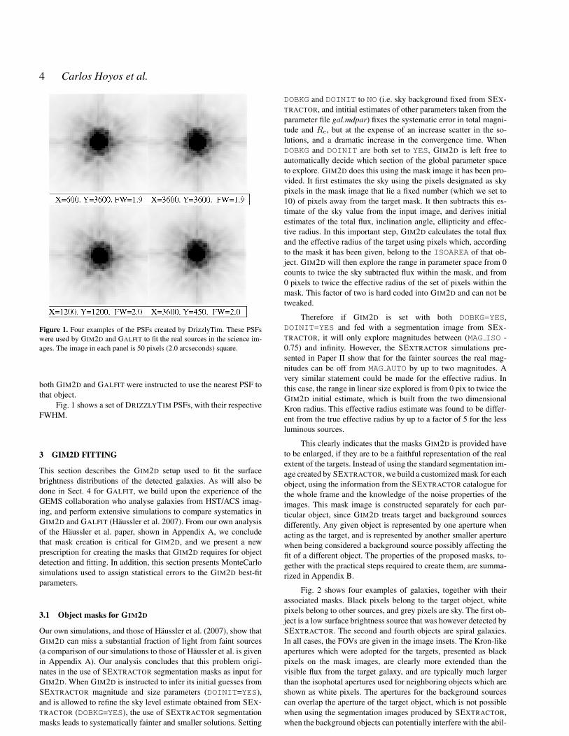
Figure 1. Four examples of the PSFs created by DrizzlyTim. These PSFswere used by GIM2D and GALFIT to fit the real sources in the science im-ages. The image in each panel is 50 pixels (2.0 arcseconds) square.

both GIM2D and GALFIT were instructed to use the nearest PSF tothat object.

Fig. 1 shows a set of DRIZZLYTIM PSFs, with their respectiveFWHM.

3 GIM2D FITTING

This section describes the GIM2D setup used to fit the surfacebrightness distributions of the detected galaxies. As will also bedone in Sect. 4 for GALFIT, we build upon the experience of theGEMS collaboration who analyse galaxies from HST/ACS imag-ing, and perform extensive simulations to compare systematics inGIM2D and GALFIT (Haussler et al. 2007). From our own analysisof the Haussler et al. paper, shown in Appendix A, we concludethat mask creation is critical for GIM2D, and we present a newprescription for creating the masks that GIM2D requires for objectdetection and fitting. In addition, this section presents MonteCarlosimulations used to assign statistical errors to the GIM2D best-fitparameters.

3.1 Object masks for GIM2D

Our own simulations, and those of Haussler et al. (2007), show thatGIM2D can miss a substantial fraction of light from faint sources(a comparison of our simulations to those of Haussler et al. is givenin Appendix A). Our analysis concludes that this problem origi-nates in the use of SEXTRACTOR segmentation masks as input forGIM2D. When GIM2D is instructed to infer its initial guesses fromSEXTRACTOR magnitude and size parameters (DOINIT=YES),and is allowed to refine the sky level estimate obtained from SEX-TRACTOR (DOBKG=YES), the use of SEXTRACTOR segmentationmasks leads to systematically fainter and smaller solutions. Setting

DOBKG and DOINIT to NO (i.e. sky background fixed from SEX-TRACTOR, and intitial estimates of other parameters taken from theparameter file gal.mdpar) fixes the systematic error in total magni-tude and Re, but at the expense of an increase scatter in the so-lutions, and a dramatic increase in the convergence time. WhenDOBKG and DOINIT are both set to YES, GIM2D is left free toautomatically decide which section of the global parameter spaceto explore. GIM2D does this using the mask image it has been pro-vided. It first estimates the sky using the pixels designated as skypixels in the mask image that lie a fixed number (which we set to10) of pixels away from the target mask. It then subtracts this es-timate of the sky value from the input image, and derives initialestimates of the total flux, inclination angle, ellipticity and effec-tive radius. In this important step, GIM2D calculates the total fluxand the effective radius of the target using pixels which, accordingto the mask it has been given, belong to the ISOAREA of that ob-ject. GIM2D will then explore the range in parameter space from 0counts to twice the sky subtracted flux within the mask, and from0 pixels to twice the effective radius of the set of pixels within themask. This factor of two is hard coded into GIM2D and can not betweaked.

Therefore if GIM2D is set with both DOBKG=YES,DOINIT=YES and fed with a segmentation image from SEX-TRACTOR, it will only explore magnitudes between (MAG ISO -0.75) and infinity. However, the SEXTRACTOR simulations pre-sented in Paper II show that for the fainter sources the real mag-nitudes can be off from MAG AUTO by up to two magnitudes. Avery similar statement could be made for the effective radius. Inthis case, the range in linear size explored is from 0 pix to twice theGIM2D initial estimate, which is built from the two dimensionalKron radius. This effective radius estimate was found to be differ-ent from the true effective radius by up to a factor of 5 for the lessluminous sources.

This clearly indicates that the masks GIM2D is provided haveto be enlarged, if they are to be a faithful representation of the realextent of the targets. Instead of using the standard segmentation im-age created by SEXTRACTOR, we build a customized mask for eachobject, using the information from the SEXTRACTOR catalogue forthe whole frame and the knowledge of the noise properties of theimages. This mask image is constructed separately for each par-ticular object, since GIM2D treats target and background sourcesdifferently. Any given object is represented by one aperture whenacting as the target, and is represented by another smaller aperturewhen being considered a background source possibly affecting thefit of a different object. The properties of the proposed masks, to-gether with the practical steps required to create them, are summa-rized in Appendix B.

Fig. 2 shows four examples of galaxies, together with theirassociated masks. Black pixels belong to the target object, whitepixels belong to other sources, and grey pixels are sky. The first ob-ject is a low surface brightness source that was however detected bySEXTRACTOR. The second and fourth objects are spiral galaxies.In all cases, the FOVs are given in the image insets. The Kron-likeapertures which were adopted for the targets, presented as blackpixels on the mask images, are clearly more extended than thevisible flux from the target galaxy, and are typically much largerthan the isophotal apertures used for neighboring objects which areshown as white pixels. The apertures for the background sourcescan overlap the aperture of the target object, which is not possiblewhen using the segmentation images produced by SEXTRACTOR,when the background objects can potentially interfere with the abil-

c© 2009 RAS, MNRAS 000, 1–22


Figure 2. Examples of the masks used by GIM2D. The “Kron-like” aper-tures devised for the 4 target objects are much larger than the aper-tures of their neighboring sources, which have an area equal to theirISOAREA IMAGE.

ity of GIM2D to measure regions outside the ISOAREA IMAGE ofthe target.

3.2 Noise model

A simple noise model is used for the fits. When GIM2D is not givena specific noise image, it builds an internal weight map based uponthe rms of the background (σbkg) and the effective gain, whichis a function of the effective exposure time of the science frames.This noise model is a transalation of the usual CCD uncertaintyequation. In our case, σbkg is taken directly from the SEXTRAC-TOR catalogue, although it is later recalculated by GIM2D in mostcases. The effective exposure time is read from the header of theHST/ACS frames.

With DOBKG set to YES, GIM2D refines the sky value givenby SEXTRACTOR, and obtains a better estimate of σbkg. This isthen used to construct the internal weight map. The sky pixels in-volved in this calculation were at least 10 pixels away from thosepixels determined to belong to the target object. The refined skyvalue is the median value of at least 30 pixels, applying a 5σ clip-ping thresholding scheme. The rms of the background obtained byGIM2D in this way is generally in excellent agreement with theσbkg initially estimated by SEXTRACTOR, both in the mean andvariance. In cases where insufficient numbers of pixels were avail-able to estimate the background rms inside the imagelet (owingto crowded fields), GIM2D defaulted to the user-supplied rms thatwas estimated by SExtractor.

3.3 Final GIM2D configuration

DOINIT was set to NO. The lower limit of the total flux was setto 0, while the upper limit was set to 10 times the automatic aper-ture flux. The Bulge-to-Total fraction was set to 1. The effective ra-dius ranged from 0.0 to 10.0 times the effective radius estimate ob-tained for a pure Sersic model of n = 2.25 of the same MUOBS andFLUX RADIUS. The ellipticity and position angle were allowed tosearch their whole ranges. The X and Y drifts were permitted torange from −10 to 10 pixels, and the residual sky value was al-lowed to go from −0.25 to 0.25. The Sersic index n was allowedto range from 0.25 to 10.0. Thus, each object had an individualizedGIM2D configuration file leading to all objects being fit by a singleSersic profile. The Metropolis temperatures are adequate for the ex-plored ranges, and expected typical changes in each iteration. In allcases, saturated pixels were rejected from the fits. The Metropolisalgorithm is given 400 iterations to cool off after achieving conver-gence (see Simard et al. 2002 for more technical detail).

3.4 Errors on the parameters and depth of the survey

Although GIM2D produces, together with its results, a set of confi-dence intervals for the fitted parameters, the error estimates repre-sent only the scale upon which the Figure-of-Merit that GIM2D

uses is expected to vary. Therefore these confidence intervalsmerely reflect how constrained the fit is. A more realistic and mean-ingful error analysis needs to investigate the extent to which theminimum of the Figure-of-Merit can drift in its parameter space.

A modest number of Monte Carlo GIM2D simulations wasrun. The purpose of these simulations is twofold. The first is tobe able to ascribe realistic statistical errors to the fits produced byGIM2D. The second purpose is to assess the surface brightness limitbeyond which it will not be possible to recover reliable structuralparameters.

10,000 model images were created using GALIMAGE withinIRAF.FUZZY. In this step, a Moffat (1969) PSF representative ofthe average properties of several non-saturated stars was used todegrade the galaxy models. MKNOISE was then used to add appro-priate Poissonian noise to this model. This blurred image was thenadded to a real ACS image which therefore provides the readoutnoise, and the bulk of the error correlation that is typical of ACSdrizzled images. The selected canvas images correspond to visits 1,15, 78, and 90 (see Paper I). SEXTRACTOR and GIM2D were run,with the same parameters, weight images and flag images as thoseused to create the SEXTRACTOR catalogue and the same experi-mental setup described above, using the Moffat PSF as the convo-lution kernel.

c© 2009 RAS, MNRAS 000, 1–22


The mean effective surface brightnesses of the models ranfrom 19.0 to 27.0, with effective radii distributed randomly inlogRe between 2.0 and 60.0 pixels. Sersic indices were randomlydistributed between 0.5 and 4.5. Ellipticities were randomly dis-tributed from 0.0 to 0.8 and position angles were unconstrained. Ofthe total number of model galaxies created, 10,000 were both de-tected by SEXTRACTOR and successfully analyzed by GIM2D; theanalysis presented in this subsection deals with these 10,000 fakesources. The remaining sources were either not detected by SEX-TRACTOR or fell in problematic areas of the image such as the CCDedges and were thus rejected.

The first step in the analysis of these simulations is presentedin Fig. 3. This figure shows the magnitude residuals against the ef-fective radius residuals, and the effective radius residuals againstthe Sersic index residuals. These relations are presented in differ-ent panels, according to the input n as indicated in the figure. Thepoints with an input 〈µ〉e brighter than 22.0 are highlighted in blue.

As expected, the residuals in total magnitude anticorrelatewith those in effective radius: where GIM2D yields a higher thanexpected luminosity, it also yields a higher than expected effectiveradius. This occurs for all Sersic indices. The oblique, green lineshows the error correlation that would preserve the mean effectivesurface brightness within one effective radius. The figure showsthat GIM2D introduces a surface brightness bias: overluminous so-lutions have fainter 〈µ〉e. The slope of this covariance is found tobe Sersic index-dependent. The contraction or expansion of the fit-ted functions with respect to the input parameters is not arbitrary,it depends on the real profile of the underlying source being fitted.Although these observations merely confirm an expected behaviourgiven the experiment being run, they are important because they al-low us to use these simulations to assess the errors on the outputparameters.

Comparable behaviour can be seen in the right panels ofFig. 3. If GIM2D finds Re higher than the real value, the output nis also higher than the real value. This happens because n is essen-tially determined by the pixels in the object wings, which are muchmore abundant and have higher weighting due to the lower Poissonnoise, thus GIM2D has to increase the model power in these wings.

In addition, the fact that the Sersic index has such a large im-pact on the behaviour of the residuals implies that this parameterhas to be included in our recipe for error assessment (see also Mar-leau & Simard 1998, their figure 11).

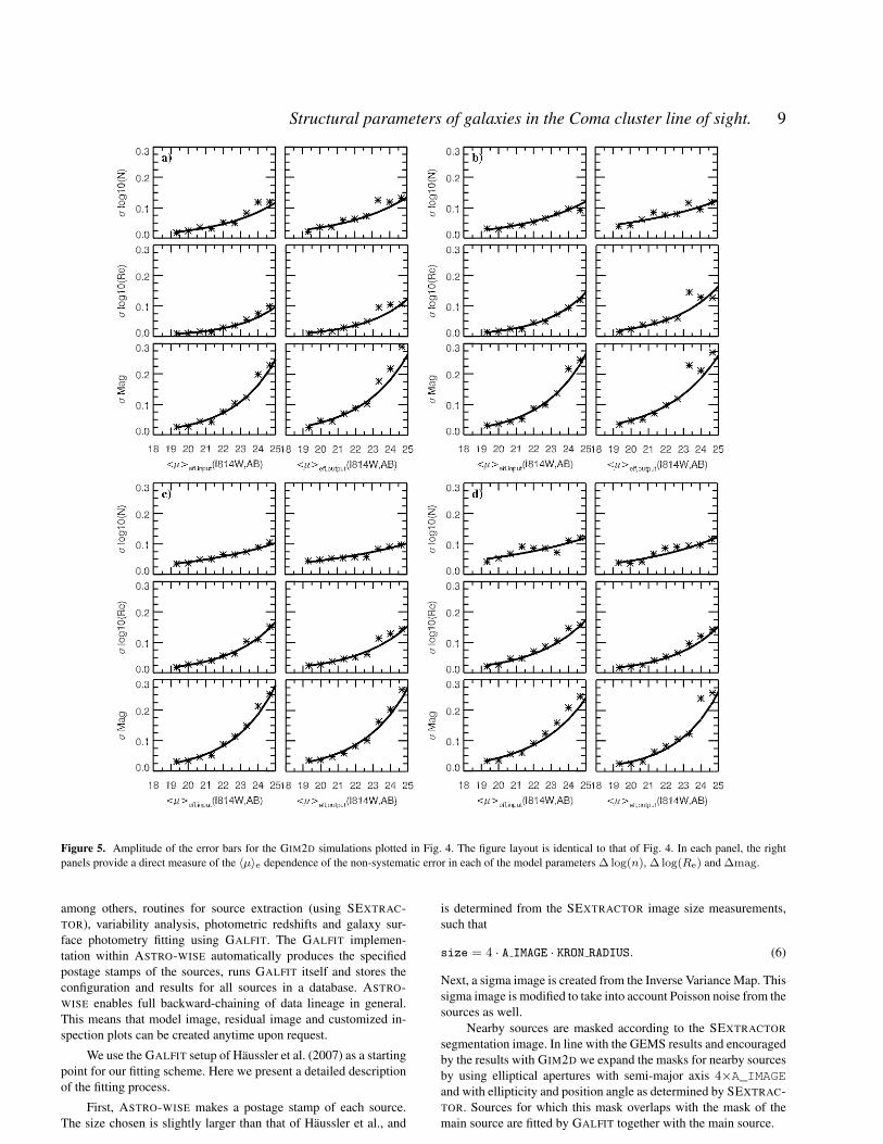
Fig. 4 shows the magnitude, effective radus and Sersic in-dex residuals against both input and output mean effective surfacebrightness for the 10000 simulations. This figure is divided intofour panels: for Sersic indices of 0.5 < n < 1.5, 1.5 < n < 2.5,2.5 < n < 3.5, and 3.5 < n < 8.0, respectively. The blacklines with error bars give the run of the median value of the resid-uals and a robust estimate of the vertical 1σ scatter of the residualsaround this latter median value. These median values of the resid-uals and their associated 1σ scatter have been calculated in equallyspaced bins in input (left panels) and output (right panels) mean ef-fective surface brightness. For clarity, the vertical 1σ scatter valuesare plotted separately in Fig. 5.

From the data presented in Figs. 4 and 5 we find that, for 〈µ〉e6 24.0, the median values of ∆ log(n), ∆ log(Re) and ∆mag (thesystematic errors) are always less than 0.05, 0.04, and 0.08, respec-tively. These values are only weakly dependent upon n, with thehighest Sersic index bin having smaller systematic errors (less than0.05, 0.03, and 0.05 respectively). For brighter surface brightness(〈µ〉e 6 21.0) these differences are lower than 0.02, 0.03, and 0.04.The widths of the distributions, which we associate with the non-

Magnitude Sersic index β α

0.5 < n < 1.5 -4.64 0.161.5 < n < 2.5 -4.22 0.152.5 < n < 3.5 -4.72 0.173.5 < n < 8.0 -5.17 0.18

logRe(G2D/Model) Sersic index β α

0.5 < n < 1.5 -5.34 0.181.5 < n < 2.5 -4.83 0.162.5 < n < 3.5 -4.43 0.143.5 < n < 8.0 -4.93 0.16

logn(G2D/Model) Sersic index β α

0.5 < n < 1.5 -3.81 0.121.5 < n < 2.5 -2.81 0.082.5 < n < 3.5 -2.74 0.073.5 < n < 8.0 -3.11 0.09

Table 1. Table of coefficients required to use Equation 5 to estimate thestatistical errors on the total magnitude, Re and n, for various ranges ofoutput n, for the GIM2D fits.

systematic error in the recovery of the input values, increase towardlower surface brightness, and are, at the faintest limit, 0.12 dex,0.15 dex, and 0.25 mag, for log(n), log(Re) and total magnitude,respectively. These values and Figures indicate that, with the use ofthe tailored masks, GIM2D is indeed able to recover the input pa-rameters accurately. The use of these customized masks and the useof the individualized search in the parameter space allows GIM2D

to have a better understanding of the galaxy flux and size. This nat-urally leads to a better fit, free from the systematic errors that weredetected by Haussler et al. (2007) and confirmed in Appendix A .

Figs. 4 and 5 indicate that it is reasonable to use the outputSersic index and 〈µ〉e to derive realistic error estimates to the totalmagnitudes, effective radii and Sersic indices. Given the modestnumber of simulations, we adopt a simple two-parameter approachbased upon the output 〈µ〉e and n. A single straight line of the form:

log σ = α× 〈µ〉e,out + β, (5)

is fit to the robust 1σ vertical scatter around the median shown inthe right panels of each quadrant of Fig. 5. Although this functionalform is expected for the magnitude uncertainties, it is also usedfor the uncertainties in Re and Sersic index for simplicity. Table 1shows the best-fit coefficients for these fits.

To assign meaningful and realistic statistical errors to anyGIM2D measurement, we first calculate the output 〈µ〉e. Next weevaluate the linear functional form given above using the coeffi-cients found in Table 1. The final uncertainty in the parameter ofinterest, as given in the structural catalogue, is the antilogarithm ofthe result.

Finally, the run of the errors with 〈µ〉e and n, given in Fig. 5and derived from the coefficients in Table 1, allow us to infer a lim-iting output 〈µ〉e beyond which GIM2D will not be able to success-fully recover the true parameters. We choose an operational limit ofan uncertainty of 0.25 mag. This limit corresponds to S/N < 5.0,and given the coefficients in the table, the corresponding limiting〈µ〉e is 24.5 mag arcsec−2. Since the magnitude is the first momentof the light distribution of any object, it will not be possible to re-liably recover the remaining structural parameters, which would behigher moments, from lower surface brightness objects.

c© 2009 RAS, MNRAS 000, 1–22


Figure 3. Effective radius residuals vs. magnitude residuals (left panels) and Sersic index residuals vs. effective radius residuals (right panels) as a function ofthe input Sersic index and 〈µ〉e. The residuals are defined as the ratio of the output value from GIM2D to the input model value. From top to bottom, the panelsinclude sources with input Sersic index 0.5 < n < 1.5, 1.5 < n < 2.5, 2.5 < n < 3.5, and 3.5 < n < 8.0, respectively. The blue dots represent pointswith input 〈µ〉e brighter than 22.0, and the black dots represent the whole pool of models created. The green line shows the location of the points should thefitting process preserve the mean effective surface brightnesses of the models. Deviations from this line indicate that GIM2D was not able to accurately retrievethe value of 〈µ〉e. Also, the slope of the clouds is correlated with the intrinsic profile of the model being fit. For galaxies with large n, it is somewhat moredifficult to reproduce the parameters of the input model. The right set of panels shows how the fits to the models expand or compress, depending on whetherthe fit overestimates or underestimates Re.

4 GALFIT FITTING

This section describes the GALFIT (version 2.0.3c) setup used tofit the program galaxies as well as the simulations carried out forerror assessment. Nearly all galaxies included in the SEXTRAC-TOR catalogue presented in Paper II were fit, except for the sourcesthat were originally buried in the extended haloes of large galaxies.

GALFIT is capable of fitting multiple galaxies simultaneously. Be-cause its χ2 minimisation algorithm is based on a gradient methodit is significantly faster than GIM2D. However the algorithm is sus-ceptible to getting stuck in a local minimum. For the fit to convergequickly to the correct values it is essential that the initial values ofthe parameters are as close to the real solution as possible.

Most initial parameters that we use for fitting are based on the

c© 2009 RAS, MNRAS 000, 1–22


Figure 4. Magnitude, effective radius and Sersic index residuals for the GIM2D simulations. This figure is divided into four quadrants, each with six panels.Top left quadrant (a) shows the residuals for simulations of galaxies with input 0.5 < n < 1.5; top right quadrant (b) simulations with input 1.5 < n < 2.5,bottom left quadrant (c) simulations with input 2.5 < n < 3.5, and bottom right quadrant (d) simulations with input 3.5 < n < 8. In each quadrant, the toptwo panels show the residuals in Sersic index as a function of input 〈µ〉e (left) and output 〈µ〉e (right) panels. The middle two panels show the residuals inRe and the bottom two the residuals in magnitude, again against input and output 〈µ〉e. The lines with vertical error bars show the run of the median value ofthe residuals; the error bars are 1.5 times the inter-quartile width of the vertical distribution. The colour coding shows the two dimensional histogram of thedensity of the underlying points, normalised along the vertical axis only. The lowest level (black) has a density >1% of the maximum, and the highest level(red) is >50% of the maximum. Intermediate shades are at 5%, 10%, 15%, 20%, 30% and 40%.

SEXTRACTOR catalogue. When fitting large numbers of galaxiesany manual intervention is extremely time consuming. Therefore,we decided to make use of ASTRO-WISE2, which provides a facilityfor the structural analysis of large datasets.

2 www.astro-wise.org

4.1 GALFIT setup in ASTRO-WISE

ASTRO-WISE is an information system and environment for largeimaging datasets, up to the Petabyte regime, with multiple usersaround Europe. In ASTRO-WISE one can archive raw data, calibratedata and perform scientific analysis storing all results. Valentijn etal. (2007) provide a technical description of the information sys-tem, and Sikkema (2009) describes the data reduction pipeline.

The scientific analysis components in ASTRO-WISE include,

c© 2009 RAS, MNRAS 000, 1–22


Figure 5. Amplitude of the error bars for the GIM2D simulations plotted in Fig. 4. The figure layout is identical to that of Fig. 4. In each panel, the rightpanels provide a direct measure of the 〈µ〉e dependence of the non-systematic error in each of the model parameters ∆ log(n), ∆ log(Re) and ∆mag.

among others, routines for source extraction (using SEXTRAC-TOR), variability analysis, photometric redshifts and galaxy sur-face photometry fitting using GALFIT. The GALFIT implemen-tation within ASTRO-WISE automatically produces the specifiedpostage stamps of the sources, runs GALFIT itself and stores theconfiguration and results for all sources in a database. ASTRO-WISE enables full backward-chaining of data lineage in general.This means that model image, residual image and customized in-spection plots can be created anytime upon request.

We use the GALFIT setup of Haussler et al. (2007) as a startingpoint for our fitting scheme. Here we present a detailed descriptionof the fitting process.

First, ASTRO-WISE makes a postage stamp of each source.The size chosen is slightly larger than that of Haussler et al., and

is determined from the SEXTRACTOR image size measurements,such that

size = 4 · A IMAGE · KRON RADIUS. (6)

Next, a sigma image is created from the Inverse Variance Map. Thissigma image is modified to take into account Poisson noise from thesources as well.

Nearby sources are masked according to the SEXTRACTOR

segmentation image. In line with the GEMS results and encouragedby the results with GIM2D we expand the masks for nearby sourcesby using elliptical apertures with semi-major axis 4×A_IMAGEand with ellipticity and position angle as determined by SEXTRAC-TOR. Sources for which this mask overlaps with the mask of themain source are fitted by GALFIT together with the main source.

c© 2009 RAS, MNRAS 000, 1–22


The implementation of the Sersic profile in GALFIT has 8 freeparameters. Of these, we leave the diskiness/boxiness parameterfixed so that all isophotes describe perfect ellipses. All other pa-rameters are left free. In addition to this, we leave the sky free,although we do not allow for any gradient in the sky. We do, how-ever, constrain n to the interval [0.5, 8.0]. Gradient based fittingmethods do require an initial guess for all parameters. Except forthe Sersic index, which we initialize as n = 1.5 for all sources,initial guesses for each source are based on parameters from theSEXTRACTOR catalogue: for Re we use FLUX RADIUS[3], fortotal magnitude we use MAG ISO. The axis ratio and position angleare initialized from ELLIPTICITY and THETA IMAGE.

ASTRO-WISE uses these parameters to write a configurationfile for GALFIT. In the case of mulitobject fitting, we determine theinput parameters for the secondary objects in the same way, withthe exception that we keep the position of the source fixed if itscentre is outside the postage stamp.

4.2 Shot-noise Simulations

Similarly to what was done for GIM2D (Sect. 3.4), an extendedset of simulations were performed. The simulations serve threemain purposes. First, they allow us to test our GALFIT setup, byidentifying biases in the fits. Second, they allow us to infer realis-tic errors of the output parameters. Like GIM2D and other fittingcodes, GALFIT tends to underestimate errors on the fitted parame-ters (cf. Haussler et al. 2007). Our simulations allow us to assign er-rors to fitted parameters which are more realistic than the standardGALFIT errors. (Our errors are still lower limits because images ofreal galaxies deviate from the perfect Sersic model with concen-tric, coaxial isophotes.) Finally, the simulations allow us to definelimits for the minimum signal-to-noise required for reasonable fits.The simulations were not designed to test the performance of GAL-FIT in crowded areas, which has already been extensively discussedby Haussler et al. (2007).

GALFIT is wrapped in ASTRO-WISE using the python lan-guage which allows for straightforward customization and scriptwriting for a specific science case. We adapted the python code inASTRO-WISE to create simulated galaxies, insert them into images,create source lists and then to run GALFIT on them. As is the casewith GIM2D, GALFIT’s ability to correctly fit a given galaxy varieswith the intrinsic parameters of the fitted galaxy. Hence, to assignerrors to the fit parameters of real galaxies we require the results ofa large number of simulated galaxies with similar output parame-ters.

In our approach we created a mock catalogue of 200,000galaxies. The parameter ranges used are listed in Table 2. Each pa-rameter samples the given range, either uniformly or uniformly inthe log as indicated in the Table. The parameter ranges were cho-sen so that the distributions of output parameters bracket the dis-tributions found in the data. When generating these parameters, weavoided the edges of the frame and applied a hard cut-off in µe toavoid any detection problems with SEXTRACTOR.

After each model galaxy had been fitted by GALFIT, the distri-butions of the differences output minus input were binned in orderto determine the variation of the errors with key output parameterssuch as magnitude, surface brightness and Sersic index. We chosesix bins in magnitude, ten bins in log(Re), two bins in ellipticityand five bins in n (600 bins in total). To minimise the uncertaintyon the errors, one would like to have as many galaxies per bin aspossible. Our 200,000 models yield ∼330 per bin, so that, eventhough for some galaxies the output bin will be different from the

parameter range #bins

x (pix) 400.0. . . 4000.0 -y (pix) 400.0. . . 4000.0 -mag 20.0. . . 25.0 6Re 2.0. . . 60.0 (log) 10n 0.5. . . 6.0 (log) 5µe <25.5 -ell 0. . . 0.8 2pos 0.0. . . 180.0 -

Table 2. Input simulation parameters of GALFIT single Sersıc galaxies. Allquantities are cast uniformly in the given range, except Re and n, whichare cast uniformly in logarithmic space. The number of bins denotes intohow many bins the range was divided for the final error assesment. In theGALFIT simulations the effective surface brightness rather than the meaneffective surface brightness was used to define the bins.

input bin and certain output bins will be more sparsely populatedthan others, the relative uncertainty on the errors (assuming theyare Gaussian) is always less than 10%.

GALFIT itself was used to generate the artificial galaxy mod-els. Although one might argue that using GALFIT to make the two-dimensional images to which itself it should fit models is doubt-ful, we stress that GALFIT has been tested extensively and that, inour opinion, it is doing at least a better job than IRAF.ARTDATA,which does not sufficiently oversample in the centres of galaxies.Our simulation setup takes into account convolution of the modelgalaxies with a DRIZZLYTIM PSF. Before injecting them into realACS observations, Poisson noise was added to these galaxies. Toavoid any crowding, we used only 100 models per ACS-frame, sothat we ended up with 2000 frames, each with 100 artificial galax-ies on top of the∼2500 sources already present. Simulated galaxieswere injected into Visit 90, because this frame is relatively emptyand on does not suffer from any missing dithers.

On each frame with simulated galaxies we ran SEXTRACTOR

using the same configuration as was used for the real data (see Pa-per II). We associated our list of simulated sources with the sourcesdetected by SEXTRACTOR by demanding that they be at most 14pixels away from the closest source in the catalogue. A small frac-tion (∼1%) of sources were not detected by SEXTRACTOR. In asmall number of cases, SEXTRACTOR can be confused by proxim-ity to or even blending with a source already present in the frame.

Results of the simulations are shown in Figs. 6 and 7. As inFig. 4, Fig. 6 shows residuals of the logarithm of the Sersic indexlog(n), the logarithm of the effective radius log(Re), and the to-tal magnitude, against input (left) and output (right) mean effectivesurface brightness 〈µ〉e. In general, the distributions of the outputparameters around the mean have non-Gaussian, extended wings.Hence, a standard RMS error does not allow for a straightfor-ward interpretation. Rather than determining the RMS of a outlier-clipped sample, we use a 95% confidence interval determined fromthe interquartile range per surface brightness or magnitude bin. Thesymmetrized intervals are used as errorbars in the plots in Fig. 6,and plotted again in Fig. 7.

The results are excellent, and, overall, similar to those ob-tained with GIM2D (Sect 3.4). Up to 〈µ〉e = 24.0, the mediandifferences, or systematic errors, are below 0.04 dex, 0.02 dex, and0.04 mag, in log(n), log(Re) and total magnitude, respectively,except for the highest Sersic index bin where the differences at〈µ〉e = 24, are always lower than 0.06 dex, 0.06 dex or 0.07 mag.The slight bias pattern that appears for 〈µ〉e > 24.0 and high Sersic

c© 2009 RAS, MNRAS 000, 1–22


Figure 6. Magnitude, effective radius and Sersic index residuals for the GALFIT simulations. This figure is organized as Fig. 4. Magnitude, effective radiusand Sersic index residuals for the GIM2D simulations. This figure is divided into four quadrants, each with six panels. Top left quadrant (a) shows the residualsfor simulations of galaxies with input 0.5 < n < 1.5; top right quadrant (b) simulations with input 1.5 < n < 2.5, bottom left quadrant (c) simulations withinput 2.5 < n < 3.5, and bottom right quadrant (d) simulations with input 3.5 < n < 6. In each quadrant, the top two panels show the residuals in Sersicindex as a function of input 〈µ〉e (left) and output 〈µ〉e (right) panels). The middle two panels show the residuals in Re and the bottom two the residuals inmagnitude, again against input and output 〈µ〉e. The lines with vertical error bars show the run of the median value of the residuals. As in Figure 4 the errorbars are given by 1.5 times the interquartile range. The colour coding shows the two dimensional histogram of the density of the underlying points, normalisedalong the vertical axis only. The lowest level (black) has a density >1% of the maximum, and the highest level (red) is >50% of the maximum. Intermediateshades are at 5%, 10%, 15%, 20%, 30% and 40%.

indices, (Fig. 6c,d), is an boundary effect of the simulation setup.Output models are brighter, and have larger Re, than the input val-ues due to the fact that input models only reach 〈µ〉e . 24.0. Theregion with output 〈µ〉e > 24.0 is only populated with models forwhich GALFIT has found a solution with fainter 〈µ〉e. Because theerrors in Re and 〈µ〉e are coupled, these models must have positiveRe residuals, as observed in the middle-right panels of Fig. 6c,d).

The run of non-systematic errors with input and output meaneffective surface brightness (Fig. 7) shows similar behaviour to

those of the GIM2D errors (Fig. 5). For a given surface brightness,GALFIT errors tend to be slightly smaller than GIM2D errors butthe differences are not meaningful, given that GIM2D values aremore uncertain owing to the lower number of GIM2D simulations.

In Table 3 we present the parameters needed to estimate theuncertainties of the GALFIT output parameters, as was previouslydone in Table 1 for GIM2D. This gives the coefficients for the fitsof Equation 5. The best-fit relations were then applied to extract the

c© 2009 RAS, MNRAS 000, 1–22


Figure 7. Amplitude of the error bars for the GALFIT simulations plotted in Fig. 6. The figure layout is identical to that of Fig. 6. In each panel, the rightpanels provide a direct measure of the 〈µ〉e dependence of the non-systematic error in each of the model parameters ∆ log(n), ∆ log(Re) and ∆mag.

error estimates for each of the Sersic parameters that are given inthe published structural catalogue.

The simulations were also used to provide a reasonable faintlimit in surface brightness that gives realistic results. A conserva-tive approach was used to define this limit, which we also set to bethe same as that applied for the GIM2D fits.

4.3 Small-size limit of GALFIT

With the discovery of 16 new Ultra Compact Dwarfs in the ComaCluster (Chiboucas et al. 2009) it is important to quantify how smallan effective radius we can measure. To see how well GALFIT canrecover radii and magnitudes for small sources, 20000 further sim-

ulations were carried out. The parameter space covered by this newset of simulations is presented in Table 4.

We find from this new set of simulations that the recov-ered effective radii are unbiased, however for very small sources(Re < 0.5 pixels) GALFIT sometimes falls back to a hard-codedlower limit of Re = 0.01 pix. This means that even for the per-fect conditions assumed in the simulations, the number of recov-ered sources that have Re around 0.5 pix will be fairly incomplete.It is very difficult for GALFIT to differentiate between a genuinepoint source and a small, yet extended, Re < 0.5 pixel source.These simulations assume perfect knowledge about the PSF, andmodel only the background contribution to the noise. Furthermore,the sources were injected on a relatively empty frame (visit 90). Tosee how well GALFIT performs on real point sources, we inspect

c© 2009 RAS, MNRAS 000, 1–22


Magnitude Sersic index β α

0.5 < n < 1.5 -1.70 0.0361.5 < n < 2.5 -1.30 0.0202.5 < n < 3.5 -1.65 0.0353.5 < n < 8.0 -2.62 0.079

logRe(GF/Model) Sersic index β α

0.5 < n < 1.5 -3.90 0.121.5 < n < 2.5 -3.57 0.112.5 < n < 3.5 -4.42 0.153.5 < n < 8.0 -3.58 0.11

logn(GF/Model) Sersic index β α

0.5 < n < 1.5 -4.09 0.131.5 < n < 2.5 -3.17 0.0922.5 < n < 3.5 -3.01 0.0843.5 < n < 8.0 -2.77 0.075

Table 3. Table of coefficients required to use Equation 5 to estimate thestatistical errors on the total magnitude, Re and n, for various ranges ofoutput n, for the GALFIT fits.

Parameter Range Remark

x 400.0 . . . 4000.0y 400.0 . . . 4000.0mag 22.0 . . . 26.5Re 0.1. . . 5.0 Logn 0.5. . . 6.0 Logµe <25.5ell 0. . . 0.8pos 0.0. . . 180.0

Table 4. Parameters of simulated galaxies for the small radii simulations.Same comments as for Table 2 apply.Reff andn are logarithmically spaced.As with Table 2 the limit in surface brightness is defined in terms of µe not〈µ〉e

the effective radii of sources in visit 19, the visit which covers thegalaxy NGC4874. A large number of the sources in this visit arethought to be globular clusters (Peng et al. 2010), which should beunresolved at the distance of 100 Mpc. Fig. 8 shows a histogramof measured effective radii for this visit. It looks as if the distribu-tion of sources is shown by a powerlaw, plus an additional group ofsources distributed around Re ∼ 0.5 pix, with a standard deviation∼ 0.3 pix. We conclude that GALFIT output giving Re ∼ 0.5 pixis likely to come from point sources. From the shape of the bluehistogram in Fig. 8 we infer that Re > 1 pixel provides a robustlower limit for GALFIT Re’s.

5 GOODNESS OF FIT INDICES

Although the Sersic model is a well-known and tested fitting func-tion, real galaxies are more complicated. They present, amongmany other features, stellar bulges, star forming regions, AGNs,spiral arms, extended haloes, and central star clusters.

In this section we define two complementary diagnostic in-dices, each designed to address in a different way the question ofwhether the Sersic model is an adequate fit, given the available data,

Figure 8. Histogram of Galfit Measurements of the Re for the sourcesfound in visits 19 and 90. The filled histogram represents the sources invisit 90, i.e. a field with few Coma galaxies. The open histogram is thehistogram of visit 19, with many Coma galaxies and globular clusters.

or whether a more complicated function or extra components arerequired. These diagnostics are calculated for all fits.

Following Blakeslee et al. (2006) we define the Residual FluxFraction (RFF) as:

RFF =

(∑i |Resi| − 0.8× σimage

)FLUX ISO

, (7)

where the summation is over all pixels within the ISOAREA of thatparticular object, |Resi| is the absolute value of residual image ob-tained by subtracting the best-fit model from the real galaxy image,and FLUX ISO is the total flux within the ISOAREA, which can betaken from SEXTRACTOR.

This index measures that part of the sum of the modulus ofthe pixels in the residual image which cannot be explained by theexperimental error. The image variance is obtained from the usualCCD equation as:

σ2image = σ2

Bkg +S

g, (8)

where S is the value of the model for that pixel, and g is the effec-tive gain, which can be found from the SEXTRACTOR parametersfor the particular image.

RFF quantifies the residual signal which cannot be explainedby arguing that the fitting codes found a suboptimal minimum. It isbest understood as a hypothesis testing procedure.

If the real galaxy had a pure Sersic profile, both GIM2D andGALFIT could find a model providing an exact fit to the galaxy.However, even in this optimal case, the errors associated with thereadout noise and photon shot noise imply that the residual imagewill not be blank. In the case of independent errors, the propertiesof the residual image would be very similar to those of gaussianwhite noise, with a spatially varying σ. The expectation value ofthe sum of the absolute values of these residuals is

∑0.8× σimage.

Therefore, the expectation value of the numerator of the RFF is 0.0,should galaxies be pure Sersic models. Since the denominator is anormalization factor, the expected value of the RFF itself is 0.0 forsuch a model. Any positive or negative deviation from a pure Sersicmodel will increase the RFF. From our own visual experience with

c© 2009 RAS, MNRAS 000, 1–22


this index, we find that fits with a RFF larger than 0.11 indicatethat a more complex fit is required. This number was agreed afterindependent experiments made by CH and RG.

The RFF diagnostic does not work well for objects with largeISOAREAS, and low 〈µ〉e. In these cases, as both the galaxy andthe model decay towards zero at large radii, the outer areas willdominate the RFF calculation, and even though the fit may havecomplicated and highly non-gaussian residuals at small radii, RFFwill still be small.

Hence we require a second diagnostic, which should be partic-ularly sensitive to the central residuals. This is calculated from thesame set of pixels within the isophotal area of the target galaxies asRFF.

This complementary parameter is the Excess Variance Index(EVI). It is defined as:

EVI =1

3×(

σ2R

< σ2image >

− 1

), (9)

where σR is the root mean square of the residuals within theISOAREA, and < σ2

image > is the mean value of the square ofthe noise within the same area. EVI gives a measure of the gran-ularity excess of the actual residuals with respect to the expectedgranularity.

For pure Sersic models, the numerator in the EVI expressionabove would simply be a sum of squares of normally distributedrandom variables with zero mean and pixel-dependent variance.The expectation value of the numerator would be, in this case, thevalue of the denominator. Hence, the parenthesized expression inthe EVI definition has an expectation value of 0.0, and strong devi-ations from 0.0 indicate that the underlying real galaxy differs sig-nificantly from a Sersic model. Given the EVI definition, such de-viations would most likely be caused by the points with the largestintrinsic standard deviations (i.e., the inner points). This makes thisindex particularly sensitive to the structure of the residuals at smallradii. The 1/3 factor in the definition of the EVI was later addedso that residual images with an EVI larger than approximately 1.0present complicated substructure in the inner parts of the fits, whilstobjects with an EVI smaller than approximately 1.0 show accept-able fits. In the end, after several iterations of this by eye calibrationcarried out by CH and RG, it was concluded that residuals with anEVI larger than 0.95 indicate complex residuals.

5.1 Comparison of the diagnostic indices

Since the RFF and EVI indices were designed to see whether asingle-Sersic fit is sufficient, it is reasonable to ask how well theGIM2D and GALFIT agree on this issue. As a first check, we plotin Fig. 9 the RFF and EVI indices of GALFIT against their GIM2D

counterparts. There is a strong correlation between the indices forthe two codes. However, there is also a small offset present, in thesense that the GIM2D indices are on average slightly higher thanthe GALFIT indices. We attribute this to a different treatment of thenoise in the calculation of the two indices (the GALFIT indices werecalculated using the sky noise from the IVM maps, whereas for theGIM2D indices we used the noise as estimated by GIM2D itself.)For high values of RFF and EVI the correlation breaks down. Espe-cially for EVI, there are galaxies where the GIM2D index is normal,but the GALFIT index is larger. In part this is the result of fitting lowS/N sources, where GALFIT has a preference for fitting a low sur-face brightness model to fluctuations in the background instead offitting the source itself.

Figure 9. Top panel: Residual Flux Fraction from GALFIT plotted againstthat from GIM2D; Lower panel: Excess Variance Index from GALFIT plot-ted against that from GIM2D.

In Fig. 10 we show histograms of the Residual Flux Frac-tion for different magnitude bins. If all sources were perfect Sersicgalaxies, these should take the form of a Gaussian, where the widthis dependent on the signal-to-noise. We find many faint sourceswith RFF < 0. We interpret this as overfitting: RFF < 0 meansthat there is less noise in the image than expected, so, the codehas modelled the noise away. For larger galaxies this problem is ofcourse less severe, as the code has to model more pixels with highersignal-to-noise, so it has less freedom.

Fig. 11 shows the calculated Excess Variance Indices, for thesame magnitude bins. Although the faint sources centre aroundzero, the brightest magnitude bins show a large fraction of highEVIs. It is only in the brightest galaxies that we can see the devia-tion from the Sersic profile (top panels), because of the high signal-to-noise and spatial resolution. For the faint sources, the data arenot good enough to detect any granularity.

These indicators will allow separation into subsamples ofgalaxies which are well represented by the Sersic function, for stud-ies of the scaling relations or for separation by morphological class,or of galaxies for which additional components, truncation or ex-tension of the light distributions show that they must be fitted withmore complex functions.

6 THE CATALOGUE

This section introduces the main result of the present paper: thecatalogue of structural parameters for the Coma-ACS survey based

c© 2009 RAS, MNRAS 000, 1–22


0.00.51.01.52.02.53.03.54.0

0.00.51.01.52.02.53.03.5

-0.2 0.0 0.2 0.4 0.6 0.8 1.0 1.2 1.4Galfit Residual Flux Fraction

0.00.51.01.52.02.53.03.5

-0.2 0.0 0.2 0.4 0.6 0.8 1.0 1.2 1.4G2D Residual Flux Fraction

Norm

alis

ed c

ounts

Figure 10. The Residual Flux Fraction calculated for our magnitude, size,and surface brightness clipped sample on the residual images of both codes.The sample is divided in three magnitude bins: 17.5-19.0 in the upper panel,19.0-22.0 in the middle panel and 22.0-25.0 in the lower panel.

0.00.51.01.52.02.53.03.54.0

0.00.51.01.52.02.53.03.5

-0.2 0.0 0.2 0.4 0.6 0.8 1.0 1.2 1.4Galfit Excess Variance Index

0.00.51.01.52.02.53.03.5

-0.2 0.0 0.2 0.4 0.6 0.8 1.0 1.2 1.4 1.6G2D Excess Variance Index

Norm

alis

ed c

ounts

Figure 11. The Excess Variance Index, see caption of Fig. 10 for moreexplanation.

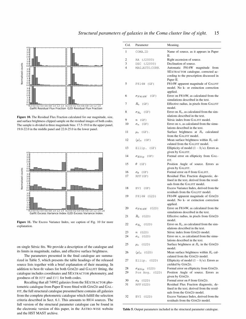
on single Sersic fits. We provide a description of the catalogue andits limits in magnitude, radius, and effective surface brightness.

The parameters presented in the final catalogue are summa-rized in Table 5, which presents the table headings of the releasedsource lists together with a brief explanation of their meaning. Inaddition to best-fit values for both GIM2D and GALFIT fitting, thecatalogue includes coordinates and SEXTRACTOR photometry, andgoodness of fit RFF and EVI for both codes.

Recalling that all 74992 galaxies from the SEXTRACTOR pho-tometric catalogue from Paper II were fitted with GIM2D and GAL-FIT, the full structural catalogue presented here contains all galaxiesfrom the complete photometric catalogue which fulfill the selectioncriteria described in Sect. 6.1. This amounts to 8814 sources. Thefull version of the structural parameter catalogue can be found inthe electronic version of this paper, in the ASTRO-WISE websiteand the HST MAST archive.

Col. Parameter Meaning.

1 COMA ID Name of source, as it appears in PaperII.

2 RA (J2000) Right ascension of source.3 DEC (J2000) Declination of source.4 MAG AUTO CORR. Automatic F814W magnitude from

SEXTRACTOR catalogue, corrected ac-cording to the prescription discussed inPaper II.

5 F814W (GF) F814W apparent magnitude of GALFIT

model. No k- or extinction correctionapplied.

6 σF814W (GF) Error on F814W, as calculated from thesimulations described in the text.

7 Re (GF) Effective radius, in pixels from GALFIT

model.8 σRe (GF) Error onRe, as calculated from the sim-

ulations described in the text.9 n (GF) Sersic index from GALFIT model.10 σn (GF) Error on n, as calculated from the simu-

lations described in the text.11 µe (GF). Surface brightness at Re calculated

from the GALFIT model.12 〈µ〉e (GF) Mean surface brightness within Re cal-

culated from the GALFIT model.13 Ellip. (GF) Ellipticity of model (1− b/a). Errors as

given by GALFIT.14 σEllip (GF) Formal error on ellipticity from GAL-

FIT.15 θ (GF) Position Angle of source. Errors as

given by GALFIT.16 σθ (GF) Formal error on θ from GALFIT.17 RFF(GF) Residual Flux Fraction diagnostic, de-

fined in the text, derived from the resid-uals from the GALFIT model.

18 EVI (GF) Excess Variance Index, derived from theresiduals from the GALFIT model.

19 F814W (G2D) F814W apparent magnitude of GIM2D

model. No k- or extinction correctionapplied.

20 σF814W (G2D) Error on F814W, as calculated from thesimulations described in the text.

21 Re (G2D) Effective radius, in pixels from GIM2D

model.22 σRe (G2D) Error onRe, as calculated from the sim-

ulations described in the text.23 n (G2D) Sersic index from GIM2D model.24 σn (G2D) Error on n, as calculated from the simu-

lations described in the text.25 µe (G2D) Surface brightness at Re in the GIM2D

model.26 〈µ〉e (G2D) Mean surface brightness within Re cal-

culated from the GIM2D model.27 Ellip. (G2D) Ellipticity of model (1− b/a). Errors as

yielded by GIM2D.28 σEllip (G2D) Formal error on ellipticity from GIM2D.29 Pos Ang. (G2D) Position Angle of source. Errors as

given by GIM2D.30 σθ (G2D) Formal error on θ from GIM2D.31 RFF(G2D) Residual Flux Fraction diagnostic, de-

fined in the text, derived from the resid-uals from the GIM2D model.

32 EVI (G2D) Excess Variance Index, derived from theresiduals from the GIM2D model.

Table 5. Output parameters included in the structural parameter catalogue.

c© 2009 RAS, MNRAS 000, 1–22


6.1 Surface brightness, magnitude and size limits

Although the two codes were used to fit all the sources detected bySEXTRACTOR in the F814W ACS images, not all of the resultingoutput parameters are meaningful and we apply limits in radius,magnitude and surface brightness to the final table, explained be-low.

The Monte Carlo simulations presented in subsections §3.4and §4.2 indicate that the uncertainty and reliability of the out-put parameters depend critically on the S/N ratio of the fittedsources. This is in turn a function of magnitude and surface bright-ness. Based upon these simulations we find that the derived pa-rameters and their errors are reliable for all sources for which:F814W < 24.5, and 〈µ〉e < 24.5.

Most galaxies for which F814W > 24.5 are likely to bebackground galaxies, and in any case are beyond the magnitudelimit of current spectroscopic surveys, so cluster membership can-not be verified, and their use in structural studies would be limited.At the distance of the Coma cluster, the apparent magnitude limitcorresponds to MF814W = −10.5, which is well within the abso-lute magnitude distribution of globular clusters.

We do find, however, that a number of galaxies with compara-tively high central surface brightness, large Re, and in some caseswith measured redshifts, fall below the surface brightness limit of〈µ〉e = 24.5. For this reason, we also include in our cataloguegalaxies with 26.0 > 〈µ〉e > 24.5, but we caution that becauseour simulations largely did not cover the parameter space occupiedby these galaxies, we have less confidence in the derived structuralparameters and their errors. For these sources for which only thecentral regions are detected, both codes are naturally forced to ex-trapolate a substantial part of the total surface brightness profile. Inthese cases, the results critically depend on the different hypothesis(e.g. constant sky) with which the codes work, and thus the derivedparameters are more uncertain.

In the final catalogue we include only sources for whichF814W < 24.5 as measured with both codes, provided that bothcodes had converged. If only one code converged then the magni-tude from that code is used. For inclusion, sources have to satisfythe surface brightness criterion for either of the codes, not both.

Besides magnitude and surface brightness cuts, we impose anRe lower limit with the aim to eliminate point sources from thecatalogue, since for these the parameters of the Sersic fit have nomeaning. From the simulations described in Sect. 4.3, we have de-cided to reject sources for which either code measures Re < 1.1pixels, which is 2σ above the mean of the distribution in Figure 8.A number of point sources remain in the catalogue, in particularsome bright, saturated stars whose wings give a larger Re. Follow-ing visual inspection of our images we estimate that < 2% of theobjects in our sample are unresolved, these are a mixture of un-rejected stars, and unresolved objects such as Coma cluster Ultra-Compact dwarfs.

6.2 Magnitude-surface brightness relation

Although we explicitly exclude any physical analysis of the struc-tural catalogue in the present paper, we give a flavour of the typesof objects included in the catalogue by showing (Fig. 12) a plot of〈µ〉e against magnitude, measured with GALFIT, for the objects inthe catalogue. In this plot, blue denotes confirmed cluster members(from the redshifts of Marzke et al. 2010), red circles confirmednon-members, and the black dots objects without measured red-shifts.

Figure 12. 〈µ〉e plotted against F814W magnitude for the objects in thecatalogue. Blue points are spectroscopically confirmed cluster members,red circles are spectroscopically confirmed not to be members. Black dotswithout a red circle are objects with no measured redshift. The diagonalline of black dots at upper right is the remaining, partly saturated, stellarcontamination.

There is a diagonal line of black (and a few red) points at theupper right, this is the residual stellar contamination, in the case ofthe bright points these stars are saturated in the ACS images, andhence have measured Re > 1.1 pixels. The cluster members forma sequence towards the lower left, with a positive correlation be-tween 〈µ〉e and luminosity. This sequence has considerable scatteras the galaxies have not been selected by morphological type nor n.Confirmed non-members (almost all background) have in generalhigher surface brightness for their apparent magnitude; however,there are also cluster members with brighter 〈µ〉e. These are com-pact ellipticals similar to those discussed by Price et al. (2009).

6.3 External Comparison

Gutierrez et al. (2004) and Aguerri et al.(2005) study the struc-tural parameters of dwarf galaxies in the Coma cluster usingground-based data obtained with the Isaac Newton Telescopeat La Palma, in the Sloan-r filter. Some of the decompositionsin these papers fit multiple components, here we only focus onthe galaxies which have bulge-to-total ratios B/T > 0.8 in theGutierrez et al. sample and the dEs (excluding the dS0s) fromthe Aguerri et al. sample. 17 galaxies from Gutierrez et al. and7 galaxies from Aguerri et al. match within 2.0 arcseconds withgalaxies in our structural catalogue. In Figure 13 we present acomparison between the effective radii Re and µe, the surfacebrightness at Re, for these galaxies. The correlation is good,with a few outliers, mostly galaxies with complex structures intheir centres which are not well resolved in the ground-baseddata.

c© 2009 RAS, MNRAS 000, 1–22


Figure 13. Comparison of our derived structural parameters with those of Aguerri et al. (2005) and Gutierrez et al. (2004). Left panel:Re in arcseconds; Rightpanel µe. Filled symbols represent our GALFIT values, and crosses our GIM2D values, as described in the legend at upper left in each panel.

7 COMPARISON BETWEEN GIM2D AND GALFIT

Both the GIM2D and GALFIT simulations have shown that thesetwo codes are capable of recovering parameters of simulated galax-ies in an almost unbiased way down to very low S/N values. How-ever, galaxies seldom consist of a single Sersic component. Thismakes a comparison between GALFIT and GIM2D for real sourcesinteresting. Even though both codes try to minimise a Figure-of-Merit (a χ2 value), there are significant differences in both theway this minimisation is achieved (Markov Chain Monte Carlo vs.Levenberg-Marquardt minimisation) and how the best fit parame-ters are determined (median value of a number of realizations inthe case of GIM2D vs. final value after a number of iterations in thecase of GALFIT ). These differences could, in principle, have an im-pact on the performance of both codes even in the case of objectssatisfying the magnitude, 〈µ〉e and Re cuts described in § 6.

7.1 Comparison of the fitted values

The top two quadrants of Fig. 14 show the difference betweenthe measured magnitudes, effective radii and Sersic indices plot-ted against the measured F814W magnitude. Quadrant (a) presentsthe results for objects with a measured Sersic index lower than2.5, whilst quadrant (b) presents the results for objects of higherSersic indices. Quadrants (c) and (d) of this figure present thesedifferences plotted against the F814W 〈µ〉e for the same divisionin Sersic index. The objects included in these plots are a subset ofthe full catalogue described in § 6. The additional constraints forinclusion in these plots are:

(i) 〈µ〉e 6 24.5(ii) RFF 6 0.11 and EVI 6 0.95(iii) 0.5 < n < 8.0

In each case the galaxies had to satisfy the constraint for bothcodes. These additional cuts guarantee that the objects included inthese plots are well measured and well represented by Sersic pro-files.

These plots show that, whenever the two codes yield a Sersicindex lower than 2.5, the observed agreement between the output

parameters is quite remarkable even for the Sersic index itself. Inthis case, the expected magnitude scatter between the two codes isaround 0.25 mag at the faintest levels, with a similar agreement inthe Re measurements.

Quadrants (b) and (d) of Fig. 14 show that in the cases inwhich the two codes measure a Sersic index higher than 2.5, thedisagreement between the two codes is larger. It is therefore moredifficult to get consistent measurements for objects with extendedwings containing a large fraction of the object’s flux. This disagree-ment between the two codes manifests itself not only as a largerscatter, but also as a systematic trend of the effective radii andSersic index residuals, when plotted against the measured surfacebrightnesses.

Whenever one code finds a brighter magnitude than the other,it also findsRe to be larger. This is in agreement with Fig. 3. This isprobably caused by differences in the sky values adopted by the twocodes. This is also the probable cause of the poorer agreement be-tween the two codes when fitting objects with high Sersic indices.For these objects, and in particular for sources that are found to bein the luminous haloes of the largest galaxies, it is very difficultto define the sky level with accuracy simply because these sourceshave a large fraction of their total flux in very extended wings andthus, any small discrepancy in the measured sky level translates intoa large difference in the final luminosity and effective radius.

Fig. 14 also shows that the scatter in the output Sersic index islarger for higher values of this index. This is caused by the fact thatmodels of high Sersic index start to converge towards a limitingr−2 profile and it is therefore very difficult to distinguish betweentwo such models.

Another discrepancy between the two codes comes from smallsources. Often these sources are fit by GALFIT with a very highSersıc index, and a half-light radius of a few pixels. These fits havea substantial portion of their light in wings which are below thedetection threshold. On the other hand, GIM2D fits these sourceswith lower Sersic indices, and the GIM2D fit is probably a morerealistic representation of the detected image.

One advantage of GALFIT is that it can model a number ofgalaxies simultaneously, leading to more consistent fits in caseswhere the target galaxy has near neighbours. GIM2D sometimes

c© 2009 RAS, MNRAS 000, 1–22


Figure 14. Quadrant (a): Magnitude, effective radius and Sersic index residuals as a function of GALFIT magnitude (left panels) and GIM2D magnitude (rightpanels). This quadrant shows results for galaxies with n < 2.5. Quadrant (b): same for objects with n > 2.5. Quadrant (c): Magnitude, effective radius andSersic index residuals as a function of GALFIT 〈µ〉e (left panels) and GIM2D 〈µ〉e (right panels). This quadrant shows results for galaxies with n < 2.5.Quadrant (d): same for objects with n > 2.5. Details of the vertical error bars and colour coding, are as in Fig. 4.

has problems with these sources as the only thing GIM2D can dowith neighbouring sources is to mask them, and that fraction of theflux from these neighbouring sources which falls outside of theirmasks will compromise the fits.

8 SUMMARY, CONCLUSIONS AND FUTURE WORK

We have fitted single Sersic models to the surface brightness dis-tributions of 74992 galaxies included in the photometric cataloguepresented in Paper II, using the two most widely used two dimen-sional galaxy fitting codes, GIM2D and GALFIT. Both codes create

a PSF convolved trial function which is then compared to the in-put science data. The PSFs used were created mimicking the mostimportant reduction steps that the science images had undergone.

Independent simulations show that both codes can achievesimilar accuracies for most cases. However, GIM2D requires amuch higher degree of intervention compared with GALFIT to pro-duce the results. This is due to the greater flexibility of GALFIT,which makes it easier for any given input image to satisfy the fit-ting hypothesis under which GALFIT works. GIM2D needs moremanual work, including the use of enlarged masks with sizes cal-culated according to our detailed Sextractor simulations, and themasking of nearby sources, to produce reliable results.

c© 2009 RAS, MNRAS 000, 1–22


These simulations, together with an additional constraintaimed at rejecting probable point sources have been used to selecta subsample of galaxies from the initial Sextractor catalogue. Thecriteria used are:

• 〈µ〉e < 26.0, where 〈µ〉e is the mean surface brightness en-closed within Re.• F814W < 24.5

• Re > 1.1 pixels

We find that 8814 objects satisfy these criteria, cross-matchingwith the redshift catalogue of Marzke et al (2010), indicates that424 of these have redshifts, of which 163 have redshifts which placethem as probable cluster members.

We have also introduced two different goodness of fit diag-nostics. The Residual Flux Fraction is an indicator of the amountof light contained in the residuals which cannot be accounted forby the per-pixel photometric errors associated with the science im-age. The Excess Variance Index measures the importance of the in-ternal structure present in luminous galaxies that the Sersic modelis unable to reproduce. These diagnostics indicate whether the sur-face brightness distributions of the fitted galaxies are well describedby the Sersic profiles, or alternatively whether it is valuable touse more complex functional forms (maybe adding a nuclear pointsource, or a bulge+disk decomposition) than the simple Sersic pro-file used in this work.

Although the Sersic fits presented here provide a good over-all description of the majority of galaxies in our sample, the spatialresolution and stability of the PSF provided by HST and ACS al-low the surface brightness to be measured accurately over a widedynamic range. A range of more complex functions have been fitto surface brightness profiles, such as the “dual power law” (Fer-rarese et al. 1994), the “Nuker Law” (Lauer et al. 1995), and thecore-Sersic profile (Graham et al. 2003; Trujillo et al. 2004). Inthe context of elliptical and spheroidal galaxies, a number of au-thors (e.g. Graham and Guzman 2003; Graham 2004; Ferrarese etal. 2006; Cote et al. 2007; Merritt & Milosavljevic 2005; Kormendyet al. 2009), have identified and measured either “extra light” or“missing light” with respect to the Sersic formalism in their pro-files. In future papers in this series we will investigate in detailthese deviations from the Sersic profile, and the correlation withkinematic properties (Emsellem et al. 2007; Cappellari et al. 2007;Krajnovic et al. 2008, van Zee et al. 2004, Toloba et al. 2009).

An alternative formalism which we will test for surface bright-ness profiles of ellipticals derives from the modified isothermalmodels of King (1962, 1966) and Wilson (1975), which are verysuccessful in reproducing the surface brightness distributions ofstar clusters, and of some, but not all, elliptical galaxies.

In the current paper we analyse only the radial surface bright-ness profile, but there is also information in the azimuthal distribu-tion, and we will undertake decompositions into disk, bulge, andnuclear components where appropriate (Andredakis et al. 1995;Balcells et al. 2007a,b), which will permit the construction of moremeaningful structural parameter diagrams for the different physicalcomponents.

We will also investigate asymmetric deviations from the ba-sic Sersic formulation of the light distribution, using techniques forparameterising galaxy surface brightness such as CAS (Conselice2003) and Gini/M20 (Lotz et al. 2004), and for detecting and quan-tifying bars (Marinova et al. 2010).

ACKNOWLEDGMENTS

We thank Dr. Luc Simard for providing the code DRIZZLYTIM.DC and AMK acknowledge support from the Science and Technol-ogy Facilities Council, under grant PP/E/001149/1. CH acknowl-edges financial support from the Estallidos de Formacion Este-lar. Fase III, under grant AYA 2007-67965-C03-03/MEC. MB ac-knowledges financial support from grants AYA2006-12955 andAYA2009-11137 from the Spanish Ministerio de Ciencia e Inno-vacion. DM was supported by grants AST-0807910 (NSF) andNNX07AH15G (NASA).

REFERENCES

Aguerri, J. A. L., Iglesias-Paramo, J., Vılchez, J. M., Munoz-Tunon, C. & Sanchez-Janssen, R. 2005, AJ, 130, 475

Andredakis, Y. C., Peletier, R. F. & Balcells, M. 1995, MNRAS,275, 874

Balcells, M., et al. 2003, ApJL, 582, L79Balcells, M., Graham, A. W. & Peletier, R. F. 2007a, ApJ, 665,

1084Balcells, M., Graham, A. W. & Peletier, R. F. 2007b, ApJ, 665,

1104Bertin, E. & Arnouts, S. 1996, A&AS, 117, 393Blakeslee, J., et al. 2006, ApJ, 644, 30Boker, T., et al. 2002, AJ, 123, 1389Caon, N., Capaccioli, M. & D’Onofrio, M. 1993, MNRAS, 265,

1013Capaccioli, M., 1989, in “The World of Galaxies”, eds. H.G. Cor-

win, L. Bottinelli (Berlin: Springer-Verlag), 208Cappellari, M. et al. 2007, MNRAS, 379, 418Carter, D., et al. 2008, ApJS, 176, 424 (Paper I)Chiboucas, K., et al. 2009, BAAS, 41, 234Chiboucas, K., et al. 2010, ApJ, in pressColless, M. M. & Dunn, A. M. 1996, ApJ, 458, 435Conselice, C.J. 2003, ApJS, 147, 1Cote, P., et al. 2007, ApJ, 671, 1456de Vaucouleurs, G. 1948, Annales d’Astrophysique, 11, 247de Vaucouleurs, G. 1957, AJ, 62, 69de Vaucouleurs, G. 1959, ApJ, 130, 728Emsellem, E., et al. 2007, MNRAS, 379, 401Erwin, P., Beckman, J. E. & Pohlen, M. 2005, ApJL, 626, L81Ferrarese, L., van den Bosch, F. C., Ford, H. C., Jaffe, W., &

O’Connell, R. W. 1994, AJ, 108, 1598Ferrarese, L., et al. ApJS, 164, 334Franx, M., Illingworth, G. & Heckman, T. 1989, AJ, 98, 538Freeman, K. C. 1970, ApJ, 160, 811Graham, A. W., Lauer, T.R., Colless, M. & Postman, M. 1996,

ApJ, 465, 534Graham, A. W., Erwin, P., Trujillo, I. & Asensio Ramos, A. 2003,

AJ, 125, 2951Graham, A. W. 2004, ApJL, 613, L33Graham, A. W. & Driver, S. P. 2005, PASA, 22, 118Graham, A. W. & Guzman, R. 2003, AJ, 125, 2936Graham, A. W. & Worley, C. C. 2008, MNRAS, 388, 1708Gray, M. E. et al. 2009, MNRAS, 393, 1275Gutierrez, C. M., Trujillo, I., Aguerri, J. A. L., Graham, A. W. &

Caon, N. 2004, ApJ, 602, 664Hammer, D., et al. 2010, ApJS, in press (Paper II)Haussler, B., et al. 2007, ApJS, 172, 615Hubble, E. P. 1930, ApJ, 71, 231

c© 2009 RAS, MNRAS 000, 1–22


Jee, M. J., Blakeslee, J. P., Sirianni, M., Martel, A. R., White,R. L., & Ford, H. C. 2007, PASP, 119, 1403

Jorgensen, I., Franx, M. & Kjaergaard, P. 1992, A&AS, 95, 489King, I. R. 1962, AJ, 67, 471King, I. R. 1966, AJ, 71, 64Koekemoer, A. M., Fruchter, A. S., Hook, R. N., & Hack, W.

2003, in “2002 HST Calibration Workshop”, eds. S. Arribas, A.Koekemoer, & B. Whitmore (Baltimore: STScI), 337

Kormendy, J., Fisher, D B., Cornell, M E. & Bender, R. 2009,ApJS, 182, 216

Krajnovic, D. et al. 2008, MNRAS, 390, 93Krist, J. 1993, Astronomical Data Analysis Software and Systems

II, A.S.P. Conference Series, Vol. 52, (eds: R. J. Hanisch, R. J.V. Brissenden, and Jeannette Banes) p. 536.

Krist, J. 2003, HST Interim Science Report 0306 (STScI)Lauer, T. R. et al. 1995, AJ, 110, 2622Lotz, J. M., Primack, J., & Madau, P. 2004, AJ, 128, 163Marleau, F. R. & Simard, L. 1998, ApJ, 507, 585Marinova, I., et al. 2010, arXiv:1002.4611Marzke, R.O., et al. 2010, in preparationMerritt, D. & Milosavljevic, M. 2005, LRR, 8, 8Moffat, A.W.J. 1969, A&A, 3, 445Mobasher, B., et al. 2001, ApJS, 137, 279Patterson, F. S. 1940, Harvard College Observatory Bulletin, 914,

9Peng, C. Y., Ho, L. C., Impey, C. D. & Rix, H.-W. 2002, AJ, 124,

266Peng, E., et al. 2010, ApJ, submitted.Reynolds, J. H. 1913, MNRAS, 74, 132Rhodes, J. D., et al. 2007, ApJS, 172, 203Rix, H.-W. et al. ApJS, 152, 163Sersic, J. L. 1963, Boletın de la Asociacion Argentina de As-

tronomıa, 6, 41Sersic, J. L. 1968, Atlas de Galaxias Australes (Cordoba: Obser-

vatorio Astronomico)Sikkema, G. 2009, PhD Thesis, Rijksuniversiteit GroningenSimard, L., et al. 2002, ApJS, 142, 1Strazzullo, V. et al. 2010, A&A in press (arXiv:1009.1423)Toloba E., et al., 2009, ApJ, 707, L17Trentham, N., et al. 2010, MNRAS in preparation.Trujillo, I., Erwin, P., Asensio Ramos, A. & Graham, A. W. 2004,

AJ, 127, 1917Trujillo, I., Graham, A.W., & Caon, N. 2001, MNRAS, 326, 869Trujillo, I., et al. 2006, MNRAS, 373, L36Valentijn, E. A., et al. 2007, Astronomical Data Analysis Software

and Systems XVI, 376, 491van der Kruit, P. C. 1979, A&AS, 38, 15van der Kruit, P. C. & Searle, L. 1981a, A&A, 95, 105van der Kruit, P. C. & Searle, L. 1981b, A&A, 95, 116van der Wel, A., Holden, B. P., Zirm, A. W.; Franx, M., Rettura,

A., Illingworth, G. D. & Ford, H. C. 2008, ApJ, 688, 48van Zee L., Skillman E. D., Haynes M. P., 2004, AJ, 128, 121van Dokkum, P. G. 2001, PASP, 113, 1420Wilson, C. P. 1975, AJ, 80, 175

APPENDIX A: COMPARISON TO GIM2D AND GALFITRESULTS BY THE GEMS COLLABORATION.

Wanting to build upon the experience obtained by other teamsin using GALFIT and GIM2D on HST/ACS data, we decidedthat the best starting point is the extensive GALFIT/GIM2D

comparison by the GEMS collaboration (Haussler et al. 2007)on mock HST/ACS observations. The GEMS collaborationprovides public access to the analysis and actual data on the web(http://www.mpia.de/GEMS/fitting paper.html).We used their Bulge0001 and Disk0001 simulated observa-tions. These contain artificial galaxies with pure Sersic profileswith n = 4 or n = 1 respectively, with appropriate Poissonnoise, on top of a noise background created by putting togetherpatches of real sky observations from different images. Thesesimulated images are created for the F850LP filter using a PSFwith a FWHM typical of this filter. The artificial galaxies cover asignificant fraction of the galaxy parameter space expected for theComa HST/ACS data, in terms of S/N ratio, total magnitude andeffective radius. Therefore our analysis of these data is useful eventhough the Coma Legacy Survey does not use the F850LP filter.

Following the work by Haussler et al. (2007) we fit a pureSersic model with a flat background. All the parameters, includingthe Sersic index, were allowed to vary freely, although the valueof the residual sky was later fixed, as explained below. The pointspread function used was identical to the one used to create themock galaxies.

For GALFIT we converged on a very similar fitting setup andbest fitting results as Haussler et al.. For GIM2D we arrived at adifferent setup and masking treatment which led to improvementsin the best fitting results.

First, GIM2D was run with its default decision algorithm onthe size of the cutout to be fitted. It was also allowed to fit and refinethe sky value by itself (DOBKG=YES) and to automatically estimateinitial values for the fitted parameters (INITPARAM=YES). TheSersic index was left as a free floating parameter. The SEXTRAC-TOR parameter configuration ensures detection of sources with aglobal signal-to-noise ratio of 20.25. The SEXTRACTOR parameterBACK SIZE was set to 512. The minimum stamp size was set to31px. This experimental configuration leads to the “recommended”setup for GIM2D. The noise model used for the GIM2D fits wasbased on the traditional CCD equation using the background σ andthe image effective gain which is ultimately regulated by the expo-sure time and reduction process.

For the Disk0001 models GIM2D produced a fit for 470 sim-ulated profiles. Figure A1 shows the results obtained by GIM2D inthis case. The upper panel presents the magnitude residuals, themiddle panel presents the ratio in effective radii, and the lowerpanel presents the output Sersic index as a function of the averagesurface brightness within a effective radius of the simulation. OurGIM2D results are shown by red crosses and the GEMS team re-sults with GIM2D by the blue circles. The general conclusion fromthis is that there are systematic trends at the faintest surface bright-ness levels, fainter than 〈µ〉e > 22.5. The scatter between fit andsimulation is smaller for our GIM2D run compared with the resultsof the GEMS team. Likely,this is caused by the fact that we maskedoverlapping sources with a value of -2 in the mask image, a situ-ation that forces GIM2D to ignore those problematic pixels. TheGEMS group did not do this.

For the Bulge0001 models GIM2D yielded a successful fit for558 simulations. Figure A2 shows the results. The general conclu-sion is that our results are an improvement on the GEMS resultsdown to a surface brightness of around z ∼ 22.5, and have asmaller scatter. However there are again systematic trends whichincrease with fainter surface brightness.

We investigated if the systematic deviations shown by theGIM2D solutions at surface brightness levels fainter than z = 23.0could be due to an inaccurate sky. To this end a number of low

c© 2009 RAS, MNRAS 000, 1–22

http://arxiv.org/abs/1002.4611

http://arxiv.org/abs/1009.1423


Figure A1. Results for GIM2D on pure exponential models. From top tobottom: magnitude residual (GIM2D minus Model), ratio of effective radius(GIM2D / Model) and Sersic index as a function of the true average surfacebrightness within an effective radius. Red crosses are our GIMD2D runs,blue crosses are the results for the same simulated galaxies from the GEMSteam.

surface brightness sources were refit. This time, we used a sky de-termination derived from a customized configuration file for SEX-TRACTOR whose main difference with the SEXTRACTOR config-uration file used in the previous fitting round is that it uses a 2048mesh for background subtraction and determination. Also, we didnot allow GIM2D to fit the sky. Furthermore the cutout size forGIM2D was increased to 25 times the default size.

Figure A3 shows the result of this test for the mock galaxiespresent in image Disk0001. Comparison with Figure A1 showsthat, using this prescription to deal with the sky level, GIM2D nolonger shows systematic offsets in magnitudes and effective radiuseven at the faintest surface brightness levels.

Figure A4 shows the result of this fitting round for the mod-els included in the Bulge0001 image. Comparison to Figure A2clearly shows that setting the sky to be equal to the sky value givenby SEXTRACTOR makes the systematic offsets in magnitudes andeffective radius to vanish even at the faintest surface brightness lev-els. The statistical errors (the scatter) are rather large however.

From the fits to the synthetic models generated by the GEMSteam comprising either pure exponentials or pure de Vaucouleursmodels, we conclude that:

• The errors in the recovery of parameters appear to be domi-nated by errors in the sky determination.• Our G2D fits show significantly reduced scatter with respect

to the G2D fits published by GEMS team. The difference can prob-ably be traced to the manual masking of intervening sources in theobject’s mask done by our team.• Increasing the cutout size used by GIM2D reduces or removes

the systematic offsets in magnitude and effective radius found whenthe default cutout size is used.• Overall, we conclude that we can use both the GALFIT and

GIM2D codes with a similar or better accuracy to that found by theGEMS collaboration.

Figure A2. Results for GIM2D on pure de Vaucouleurs models. From topto bottom: magnitude residual (GIM2D minus Model), ratio of effectiveradius (GIM2D / Model) and Sersic index as a function of the true averagesurface brightness within an effective radius. Red crosses are our GIMD2Druns, blue crosses are the results for the same simulated galaxies from theGEMS team.

Figure A3. Results for GIM2D on pure exponential models of low surfacebrightness, using our own sky determination (see text). From top to bot-tom: magnitude residual (GIM2D minus Model), ratio of effective radius(GIM2D / Model) and Sersic index as a function of the true average surfacebrightness within an effective radius. Red crosses are our GIMD2D runs,blue crosses are the results for the same simulated galaxies from the GEMSteam.

APPENDIX B: CREATING OBJECT MASKS FOR GIM2D

We provide a detailed recipe for producing object masks for GIM2D

that solves the missing flux problem that appears when standardSEXTRACTOR segmentation masks are used in GIM2D.

(i) The aperture for the target should ideally be equal to theKron aperture of an object with the same FLUX RADIUS and nthat would be measured if the observations had infinite S/N ratio.The elongation and position angle of this aperture would ideallybe equal to those of the real object. The pixels within this aper-

c© 2009 RAS, MNRAS 000, 1–22


Figure A4. Results for GIM2D on pure de Vaucouleurs models of low sur-face brightness, using our own sky determination (see text). From top tobottom: magnitude residual (GIM2D minus Model), ratio of effective ra-dius (GIM2D / Model) and Sersic index as a function of the true averagesurface brightness within an effective radius. Red crosses are our GIMD2Druns, blue crosses are the results for the same simulated galaxies from theGEMS team.

ture should be flagged as 1 in the mask file so that GIM2D recog-nizes them as belonging to its target object. This aperture is cal-culated from the SEXTRACTOR measurements. FLUX RADIUS,THETA IMAGE and ELONGATION were taken directly from theSEXTRACTOR catalogue. MUOBS is a SEXTRACTOR based esti-mate of effective surface brightness of that particular detection, ob-tained as if MAG AUTO were the total magnitude and the 50% ofFLUX RADIUS were the real effective radius. It is thus an esti-mate of the effective surface brightness. The 5th degree polyno-mials used in the SEXTRACTOR simulations presented in Paper IIwere then used to estimate empirically the effective radius of thesource. This effective radius estimate is then converted into a Kronaperture using the relationship between Re and R1 (the S/N =∞Kron aperture in units of the effective radius) and n. n = 2.5 isassumed where n is undefined. Although the aperture defined inthis way leaves out a finite fraction of the total flux from the targetmodels outside the mask, this magnitude offset is 0.1 mag in theworst case. For this reason, the initial flux estimate will be around0.1 mag fainter than the true integrated flux. As above, a very simi-lar statement can be made about the initial effective radii estimates.Using this customized mask, GIM2D has a realistic opportunity tomeasure 100% of the target object total flux and size, whereas withthe default SEXTRACTOR segmentation image, this is not true.

(ii) The apertures for the background sources are elliptical aper-tures, with an area given by the ISOAREA IMAGE SEXTRACTOR

measurement. The elongation and position angles of these ellipsesare also taken from the SEXTRACTOR measurements. These pixelsare flagged as -2 so that GIM2D ignores these pixels in all cal-culations. GIM2D is therefore blind to the innermost regions of thebackground sources. Thus only the outer regions of the backgroundsources contribute to the sky level affecting the galaxy under study.In the case of an overlap between target and background object pix-els, the pixels are assigned to the background object as includingthem in the target would potentially compromise the fit.

(iii) Finally, pixels not belonging to the target or to the back-

ground sources are flagged as 0, so that GIM2D regards these pixelsas sky.

In a few cases, for instance, with objects with close neigh-bours or near to the CCD edges, SEXTRACTOR did not providemeasurements of MAG AUTO and FLUX RADIUS. In these casesMUOBS is estimated by spreading the light encircled in the isopho-tal area of the object (ISOAREA IMAGE) uniformly in an aperture

with a radius equal to 12×√

ISOAREA IMAGEπ

. This was found tobe somewhat brighter than a measured MUOBS, although the finalapertures obtained were similar in size.

The size of the poststage stamp over which GIM2D has towork is an integral part of the suggested solution. The quantityFRAD MOD amounts, in the vast majority of the cases, to 50%of FLUX RADIUS, as calculated by SEXTRACTOR. For the ob-jects where SEXTRACTOR could not calculate FLUX RADIUS,FRAD MOD is half of the radius of the circle with an area equalto ISOAREA IMAGE, which always does exist.

The number YFX(MUOBS) is given by the empirical rela-tion between the 50% FLUX RADIUS and the input effective ra-dius that is appropriate for sources with a high n. For reasonableSersic indices YFX(MUOBS) is given by the fifth-order polyno-mial in the mean observed surface brightness MUOBS, presented inpaper II. The final size of the post stamps imagelets extracted is7.0× FRAD MOD×YFX(MUOBS) on a side.

c© 2009 RAS, MNRAS 000, 1–22

Documents

The HST/ACS Coma Cluster Survey - III. Structural parameters of galaxies using single Sérsic fits★