KWAME NKRUMAH UNIVERSITY OF SCIENCE AND TECHNOLOGY,

KUMASI

INSTITUTE OF DISTANCE LEARNING

THE IMPACT OF FOREIGN DIRECT INVEESTMENT (FDI) ON

ECONOMIC PERFORMANCE IN GHANA

BY

BABA ADAM, CA, BCom (Hons.),

A THESIS SUBMITTED TO INSTITUTE OF DISTANCE LEARNING, KWAME

NKRUMAH UNIVERSITY OF SCIENCE AND TECHNOLOGY (KNUST) IN

PARTIAL FULFILMENT OF THE REQUIREMENT FOR THE AWARD OF

MASTERS OF SCIENCE IN INDUSTRIAL FINANCE AND INVESTMENT

DEGREE

MAY 2015

i

DECLARATION

I hereby declare that this thesis is my own work and effort and that it has not been submitted

anywhere for any award in this and any university. All references used in the work have been fully

acknowledged.

I bear sole responsibility for any shortcomings.

Baba Adam Signature ……………… Date………………

(PG 8678412)

Mr. Mustapha Immurana Signature……………….. Date……………….

(SUPERVISOR)

Prof Isaac Kwame Donwti Signature …………………. Date ………………….

Director, Institute of Distance Learning (IDL)

ii

DEDICATION

I dedicate this thesis to my wife, Fulera, who has been a constant source of support and

encouragement during the challenges the masters program and life. I am truly thankful for

having you in my life. I also dedicate this work to my parents and guardians, who have

always loved me unconditionally and whose good examples have taught me to work hard for

the things that I aspire to achieve.

Finally to my children Faheem Wunpini and Fawzan Faako, I say big thanks to you guys for

your patients and support during this course.

iii

ACKNOWLEDGEMENT

My special thanks go to Almighty Allah for good health, prosperity and sense of Reasoning. I

would like to acknowledge special role Supervisor Mr.Mustapha Immurana, played in

producing this master piece. Again, I take this opportunity to express my profound gratitude

to him for the support, encouragement and leadership provided during this difficult but

enduring time. You have indeed been a tremendous mentor for me. I would like to thank you

for your tolerance and zeal to demand the best. Your advice on both research as well as on

my career development have been priceless also, wish to thank the research seminar

committee members,, Dr.Sackyi, Dr.Oteng-Abayie, and Dr.Yusif for the critique, advice and

encouragement during the period.

A special thanks to my brother, Muazu who took time off his busy schedule to offer technical

and advisory services to me. Words cannot express how grateful I am to you.

Finally thanks goes to all my friends, course tutors and course mates who supported me in

writing, and encouraged me to strive towards my goal.

I say may Allah richly bless us all.

iv

ABSTRACT

The past few decades have witnessed the inflows of foreign direct investment (FDI) into

developing economies including Ghana. Advocates for increased FDI inflows are done on the

premise that FDI significantly contribution to fiscal development through by augmenting the

supply of funds for investment thus promoting capital formation in host countries. However,

opponents of FDI have advanced their argument largely on its impact on the balance of

payments and trade deficit of host countries. They argue that if investors import more than

they can export, FDI would end up worsening the trade situation of the country and

consequently growth. This thus calls for the need for further research on FDI – growth nexus.

In addition to assessing the impact of FDI on economic growth in Ghana, this study aims at

examining the impact of FDI on the various sectors of the economy as well as the

contribution of FDI to trade volume. Relying on annual data spanning 1980 to 2013 and

employing Johansen cointegration and vector error correction model (VECM), the study

found a positive and significant impact of FDI on economic growth. At the sectoral level,

while its effect on the agriculture sector is negative, FDI inflows positively affect the value

additions of the industrial sector. Its impact on the service sector is however less significant.

Further results show that, in the long-run, while FDI, gross fixed capital formation and trade

openness positively affects trade volumes, the effect of exchange rate is negative and

significant suggesting that currency depreciation hurts trade volumes. However, in the short-

run only trade openness drives trade and inflation does not matter in determining the amount

of trade volumes both in the short- and the long-run. In addition to maintaining a continued

trade relations aimed at attracting more FDI inflows, there is the need for the government to

ensure that constraints in agriculture sector – namely inadequate road network, low

commodity prices at the international market and lack of credit to farmers – are eliminated in

order to increase productivity so that a self-sustained value addition could take place.

v

LIST OF TABLES

TABLE PAGE

Table 1 Summary of Descriptive Statistics 46

Table 2 Augmented Dickey-Fuller (ADF) Unit Root Test Result 47

Table 3 Phillips-Perron (PP) Unit Root Test Results 48

Table 4 VAR Lag Order Selection 49

Table 5 Unrestricted Co-integration Rank Test (Trace) 50

Table 6 Unrestricted Co-integration Rank Test (Maximum Eigenvalue) 50

Table 7 Impact of FDI on real GDP 51

Table 8 VECM Results 54

Table 9 VAR Lag Length Selection Criteria 56

Table 10 Unrestricted Co-integration Rank Test (Trance) 57

Table 11 Unrestricted Co-integration Rank Test (Maximum Eigenvaluue) 57

Table 12 Impact of FDI on Agric Sector 58

Table 13 VECM Results 60

Table 14 VAR Lag Order Selection Criteria 61

Table 15 Unrestricted Co-integration Rank Test (Trance) 62

Table 16 Unrestricted Co-integration Rank Test (Maximum Eigenvaluue) 62

vi

Table 17 Long-Run Impact of FDI on the Service Sector 63

Table 18 VECM Results 65

Table 19 VAR Lag Order Selection Criteria 66

Table 20 Unrestricted Co-integration Rank Test (Trance) 66

Table 21 Unrestricted Co-integration Rank Test (Maximum Eigenvaluue) 67

Table 22 Long-Run Impact of FDI on the Industrial Sector 68

Table 23 VECM Results 69

Table 24 VAR Lag Order Selection Criteria 71

Table 25 Unrestricted Co-integration Rank Test (Trance) 72

Table 27 Long-run Impact of FDI on Trade volume 73

Table 28 VECM Results 74

vii

LIST OF FIGURE

FIGURE PAGE

Figure 1 Trends in FDI inflows (1980 – 2013) 31

viii

LIST OF ABREVIATIONS

ADF Augmented Dickey-Fuller

ADI African Development Indicators

ECT Error Correction Term

ERP Economic Recovery Programme

FDI Foreign Direct Investment

GDP Gross Domestic Product

GMM General Method of Moment

IMF International Monetary Fund

NEPAD New Partnership for African’s Development

OECD Organization for Economic Co-operation and Development

OLS Ordinary Least Squares

PP Phillip-Perron

SIC Schwarz Information Criterion

SSA Sub-Sahara Africa

TNCs Trans-National Corporations

UNCTAD the United Nations Conference on Trade and Development

VAR Vector Autoregression

VECM Vector Error Correction Model

WDI World Development Indicators

ix

TABLE OF CONTENTSDECLARATION................................................................................................................................... ii

ACKNOWLEDGEMENT.................................................................................................................... iv

ABSTRACT..........................................................................................................................................v

LIST OF TABLES................................................................................................................................vi

LIST OF FIGURE...............................................................................................................................viii

LIST OF ABREVIATIONS..................................................................................................................ix

TABLE OF CONTENTS.......................................................................................................................x

CHAPTER ONE....................................................................................................................................1

1.1 Background.................................................................................................................................1

1.2 Problem Statement.......................................................................................................................3

1.3 Objectives of the Study................................................................................................................3

1.5 The Scope of Study......................................................................................................................4

1.6 Justification of the Study.............................................................................................................4

CHAPTER TWO...................................................................................................................................6

LITERATURE REVIEW..................................................................................................................6

2.1 Introduction.................................................................................................................................6

2.2 Definition of FDI.........................................................................................................................6

2.2.1 Types and Forms of FDI.......................................................................................................8

2.2.2 FDI Classification.................................................................................................................8

2.3 Theories of FDI...........................................................................................................................9

2.3.1 The Dependency Theories and FDI......................................................................................9

2.3.2 Location Theory..................................................................................................................10

2.3.3 The Eclectic Theory............................................................................................................10

2.3.4 Market Power and Competition Theory..............................................................................11

2.3.5 Neoclassical Theory............................................................................................................12

2.3.6 FDI Theory on Capital Accumulation.................................................................................13

2.3.7 Internalization Theory.........................................................................................................13

2.4 Why FDI Is Seen As Important For Africa................................................................................14

2.5 The Potential Problems Associated With FDI...........................................................................15

2.6 Trends in FDI Inflows to Ghana (1980 – 2010).........................................................................16

2.7 Empirical Literature Review......................................................................................................19

2.8 Conclusion.................................................................................................................................25

CHAPTER THREE.............................................................................................................................26

x

METHODOLOGY..............................................................................................................................26

3.1 Introduction...............................................................................................................................26

3.2 Data Sources..............................................................................................................................26

3.3 Description of Variables............................................................................................................26

3.3.1 Real GDP (RGDP)..............................................................................................................26

3.3.2 Gross Fixed Capital Formation (% of GDP).......................................................................26

3.3.3 Exchange Rate (EXR).........................................................................................................27

3.3.4 Foreign Direct Investment (FDI), Net Inflows (% of GDP)................................................27

3.3.5 Inflation (INFL)..................................................................................................................27

3.3.6 Agriculture, Value Additions (Constant 2005 US$)............................................................28

3.3.7 Industry Value Additions (Constant 2005 US$)..................................................................28

3.3.8 Service Value Additions (Constant 2005 US$)...................................................................28

3.3.9 Trade Openness (TRADE)..................................................................................................29

3.3.10 Trade Volume (TVOL).....................................................................................................29

3.4 Models Specification.................................................................................................................29

3.5 Unit Root Testing......................................................................................................................30

3.6 Cointegration.............................................................................................................................31

3.7 Conclusion.................................................................................................................................34

CHAPTER FOUR...............................................................................................................................35

RESULTS AND DISCUSSION..........................................................................................................35

4.1 Introduction...............................................................................................................................35

4.2 Descriptive Statistics.................................................................................................................35

4.3 Unit Root Test Results...............................................................................................................36

4.3.1 The Augmented Dickey-Fuller (ADF)................................................................................37

4.3.2 Phillips-Perron (PP)............................................................................................................38

4.4 Impact of FDI on Economic Growth.........................................................................................39

4.5 Impact of FDI on the Agricultural Sector..................................................................................48

4.6 Impact of FDI on the Service Sector..........................................................................................54

4.7 Impact of FDI on the Industrial Sector......................................................................................63

4.8 Impact of FDI on the Trade Volume..........................................................................................71

4.9 Conclusion.................................................................................................................................77

CHAPTER FIVE.................................................................................................................................79

FINDINGS, CONCLUSION AND RECOMMENDATIONS.............................................................79

5.1 Introduction...................................................................................................................................79

xi

5.2 Summary.......................................................................................................................................79

5.3 Conclusion.....................................................................................................................................81

5.4 Recommendations.........................................................................................................................81

APPENDIX.........................................................................................................................................86

xii

CHAPTER ONE

INTRODUCTION

1.1 Background

The impact of Foreign Direct Investment (FDI) in stimulating economic advancement and

expansion in Africa cannot be overlooked. The growth of international production is

determined by economic and technological forces. It is also driven by the on-going

liberalization of FDI and trade policies. In this background, globalization offers an

unparalleled opportunity for developing countries to achieve quicker economic growth

through trade and investment. Most developing nations see FDI as universal antidote to the

problems of transition and under-development; hence enhanced FDI flows were particularly

encouraged. This situation was seen in the middle of the 1980s, when world FDI started to

increase sharply. Because of the significant role that FDI plays in the global economic

environment, it has become one of the hottest issues in the world economy today. FDI has

emerged as the most important source of external resource flows to many African countries

with investible resources to finance long-term investment (Ibrahim .A (2005).

Apart from making investible funds available, FDI inflows to developing countries is

assumed to produce externalities through technology transfer and spill-over effects (Carkovic

and Levine, 2002), which have long-term effects on the economy. It implies that FDI inflows

enable the host countries to achieve investment that may exceed their own domestic savings

and enriches capital funding. It is on these grounds that Asafu-Adjaye (2005) argues that FDI

plugs the savings-investment gap in the host country and concludes that a foreign corporate

presence generate positive externalities such as improvement in human capital and local

institution.

1

Also, United Nation (2005) argues that FDI is seen as a main source of getting the essential

funds for investment henceforward most African countries offer incentives to encourage FDI.

The global recognition in the growth improving effects of FDI is authenticated by the scuffle

of governments to attract foreign investment with all policy incentive packages.

As pointed out by Khan (2007), the role of FDI has been generally accepted as a growth-

enhancing cause in unindustrialized countries. It is on this background that policymakers

especially in emerging nations have come to conclusion that FDI is needed to enhance

economic growth in their respective economies. Thus, the impact of FDI on economic growth

cannot be over-emphasized. It is therefore not surprising that it is echoed in the New

Partnership for African’s Development (NEPAD) to be a key resource for the translation of

NEPAD’s vision of growth and development into reality Funke and Nsouli, (2003).

Notwithstanding all the positive contribution to economic growth, some researchers maintain

that FDI has negative impact and may perpetuate the dependency relationship between

advanced and developing economies. Todaro and Smith (2005) argue that FDI may weaken

balance of payment as profits are repatriated and may have negative effects on the growth

prospects of the host country’s economy if they result in substantial reverse flows in the form

of remittances of profits and more efficient allocation of resources.

Zhang (2006) suggests that FDI might actually lower domestic savings and investment

therefore FDI might decrease the growth rate of Gross Domestic Product (GDP). Another

negative impact is the increasing inequalities in national development. Townsend (2003)

contends that the relationship between FDI and economic growth is not so clear. There are

different views by researchers on the contribution of FDI to economic growth, based on

theoretical and analytical findings. Less developed countries see FDI as a very important tool

for economic growth but some scholars claim that the contribution of FDI to economic

development is not as pronounced as most people believe. Somo (2008) argues that the

2

empirical evidence available provides mixed result countries and firms to identify their

absorptive capacity in order to reap the benefits.

1.2 Problem Statement

Whiles researchers like Carkovic and Levine (2002), Khan (2007), and Asafu-Adjaye (2005)

believe that FDI may perhaps contribute to economic development and growth, other

researchers such as Zhang (2006) and Todaro and Smith (2005), believe that FDI could retard

economic intensification in underdeveloped countries. Again, pragmatic studies on the impact

of FDI on fiscal expansion and development according to Somo (2008) have produced mixed

results. Also noted to have researched on this area is; Townsend (2003) contends that the

correlation connecting FDI and economic growth is not so clear. This therefore concludes

that, the impact of Foreign Direct Investment on economic growth and development is

inconclusive necessitating further research efforts in this direction. Given the fact that,

developing nations governments including the Ghanaian government are striving hard to

attract FDI in order to stimulate economic growth and development in their respective

nations, again, previous researchers like Asafu-Adjaye (2005), Ibrahim. A (2005) did not

extend their study to cover; agriculture sector, service sector and industrial sector of the

economy, but rather limited it to mining and manufacturing sub sectors. Hence, it is

imperative to conduct an empirical study to find out whether FDI actually leads to economic

growth and development in Ghana and its impact on the selected sectors.

1.3 Objectives of the Study

The general objective of the study is to measure the performance of FDI on the economy.

The specific study would want:

1. To determine the impact of Foreign Direct Investment on economic growth in Ghana

2. To analyse the role of Foreign Direct Investment on the various sectors of the

economy

3

3. To analyse the impact of FDI on trade volume in Ghana

1.4 Research Questions

In other to achieve the above objectives, the study will seek to answer the following research

questions;

1. What is the impact of FDI on the economic growth of Ghana?

2. What are the impacts of FDI on the various sectors of the Ghanaian economy?

3. Does FDI contribute to trade in Ghana?

1.5 The Scope of Study

The study is a case study on the economy of Ghana and time series data from spanning 1980

to 2013 were gleaned from the World Development Indicators (WDI) of the World Bank and

African Development Indicators (ADI). The study employed Augmented Dickey-Fuller

(ADF), Philip-Perron (PP), Johansen cointegration techniques and the vector error correction

model (VECM) to achieved objectives of the study.

1.6 Justification of the Study

Practical proof on the impact of FDI on economic growth and development is still

inconclusive. As such, it requires a detailed study in order to shed light on its dynamics and

nature. The rationale of this work is to understand and assess the control foreign capital has

on the economy of emerging countries, with focus on FDI.

This research after its completion therefore would help illustrate how FDI contribute to

economic growth and development. There exist a plethora of empirical studies on FDI –

growth nexus although findings are still mixed and inconclusive. However, sectoral analysis

of the impact of FDI in Ghana is almost non-existent. By carefully studying these metrics,

this work contributes significantly to the scanty literature especially at the sector level

analysis. Findings from the study is expected to bring up issues to the attention of policy

4

makers and industry captains to appreciate the real contributions and impact of FDI in the

development and economic growth agenda of Ghana by focusing on the various sectors.

1.7 Organization of the Study

The research is structured into five sequential chapters. Chapter one deals with the

background of the study, justification of the study, problem statement, research objectives,

and research questions, scope of the study and organization of the study. The second Chapter

which is the review of literature tackles both theoretical and empirical literature. While

chapter three provides the detailed methodology, chapter four presents results and discussion

of the study. Chapter five however summarizes and concludes the study with some

recommendations for policy.

5

CHAPTER TWO

LITERATURE REVIEW

2.1 Introduction

While the general objective of this chapter is to present a summary of Ghana’s growth

patterns and FDI inflows, this chapter is divided into three different but related parts. The

introduction part provides the definition, types and composition of FDI and some key

theoretical propositions on FDI inflows in host countries. The second section provides an

analysis of trends of FDI inflows with special emphasis on Ghana. The third section presents

the empirical arguments as based on the practical studies on the role of FDI on growth using

various econometric and cross–country time series regressions.

2.2 Definition of FDI

FDI does embrace the entire investments portfolio across boundaries. There are a few

characteristics that position Foreign Direct Investment different from other intercontinental

trade or investments and these are debated below.

Foreign Direct Investment is a particular kind of foreign capital, as different to domestic

investment or foreign governments. FDI does not include loan capital and or grant provided

by international organizations, nor does it automatically include portfolio investments such as

stocks, debentures and bonds purchased by foreign investors. What makes investment

“direct” as different from other forms of foreign capital is the concept of managerial control

over a project in which foreign capital participates. FDI comprises activities that are

controlled and organized by firms (groups of firms) outside the nation in which they are

headquartered and where their principal decision makers are located. The United Nations

Conference on Trade and Development (UNCTAD) World Investment Report (2008),

6

describes FDI as “an investment concerning a long-term relationship and replicating a lasting

interest and control by a resident entity in one economy (foreign investor or parent enterprise)

in an enterprise resident in another economy other than that of the foreign direct investor

(FDI enterprise or foreign affiliate)”. The World Bank defines it as an investment made to

acquire lasting management (usually at least 10% of voting stock) in an enterprise operating

in a country other than that of the host investor (cited in Gillis et al, 2001: 522).

The International Monetary Fund (1999) explains FDI as investment that is made to obtain a

permanent interest of a resident entity in one economy (direct investor) in an entity resident

in another economy (direct investment enterprise) cover all transactions between direct

investors and direct investment enterprises. That is, direct investment covers the initial

transaction between the two and all subsequent transactions between them and among

affiliated enterprises; both incorporated and unincorporated. While OECD’s standard

definition of FDI identifies FDI’s objective as obtaining a permanent interest by a resident

entity (direct investor) in one economy other than that of the investor (direct investment

enterprise). The permanent interest implies the existence of a long-standing relationship

between the direct investor and the enterprise and a significant degree of influence on the

management of the enterprise. Direct investment involves both the initial transaction between

the two entities and all subsequent capital transactions between them and among affiliated

enterprise; both incorporated and unincorporated (OECD, 1996).

FDI is a direct investment into production or business in a country by an individual or

company of another country, either by buying a company in the target country or by

expanding operations of an existing business in that country. FDI is in contrast to portfolio

investment which is a passive investment in the securities of another country such as stocks

and bonds (Investopedia, 2013).

7

2.2.1 Types and Forms of FDI

FDI means the capital mobility from one country to a host country. This occurs in ways as

creation of a subsidiary of a company- green field investment or the extension of already

existing companies- mergers and acquisitions. From multinational company’s viewpoint,

there are two types of FDI, export-oriented and domestic-market oriented. The export-

oriented categories are also called vertical FDI where the inflows into a host country are only

made up of raw materials for the production of finished products. Such FDIs are usually

motivated by availability of cheap labour in the host country thus reducing their production

cost. Domestic market oriented known as horizontal FDI on other hand, produces goods and

sells them to the host market taking advantage of the host population.

2.2.2 FDI ClassificationThe organization for economic co-operation and development (OECD, 2000) categorised FDI

into four categories as follows;

a) Equity Joint Ventures (EJVs): This includes joint investment by foreign and Ghanaian

companies. Under this category, profits are shared based on the stake in the joint

venture. This class also encourages technological transfer in the domestic companies.

b) Wholly Foreign-Owned Enterprises: these are limited liability corporations organized

by foreign nationals and capitalized with foreign funds. Wholly owned companies are

often used to produce the goods and services for export.

c) Joint exploration: This kind of FDI takes place in the early stage in the Country

development and refers to projects mainly unimportant in order to explore the market

of the country.

d) Mergers and acquisition of unrelated: the majority investment has engaged the

structure of attainment of existing assets rather than investment in new assets

8

(Greenfield). Mergers and acquisitions have become a popular mode of investment of

companies wanting to protect, consolidate and advance their positions by acquiring

other companies that will enhance their competitiveness. Mergers and acquisitions are

explained as the acquisition of more than 10% equity share, involved in transfer of

possession from home based investor to overseas hands, and do not create new

productive facilities. Based on this definition, Mergers and acquisitions raise

particular concerns for developing countries, such as the extent to which they bring

new resources to the economy, the denationalization of domestic firms, employment

reduction, loss of technological assets, and increased market concentration with

implications for the restriction of competition (Fung, 2002).

2.3 Theories of FDIThe discussion of the theories of FDI boarders on the organizational aspect of international

trade and behavioural aspects of the enterprise involved. It also includes the institutional

consideration of the receiving countries. The growth in global trade can be traced from

industrialization and internationalization of production. This internalization of production

leads to setting up of offshore production plant by undertaking FDI. The link between these

schools of thought to explain FDI flows are analyzed in the theories that are discussed below

2.3.1 The Dependency Theories and FDIThe dependency school pay more attention on the effects of FDI in emerging nations.

According to the dependency theory, under-developing nations are oppressed as they take on

intercontinental business in the form of deteriorating exchange rates and in expatriation of

profit by trans-national corporations (TNCs). As far as the structuralist view is concerned, the

core-periphery relationship leads to the utilization of the periphery by the centres through the

extraction of resources from the former (Wilhelm, 1998). These dependency theories suggest

that developing countries can escape from their underdeveloped state by retreating from

9

international investment and trade and rather concentrate on intra-bloc trade. These theories

do not currently influence trade policies, because FDI and portfolio investment are

indispensable for economic growth and development. The savings gap is then filled by

external sources and especially FDI inflows. It is therefore not possible for developing

countries to retreat from international investment without harming themselves (Wilhelm,

1998).

2.3.2 Location Theory

Opposing to the industrial organization approach, location theory drew attentions on country-

specific features. It explained Foreign Direct Investment performance in terms of relative

economic conditions in investing and host countries, and considered locations in which FDI

would work better. This approach includes two subdivisions: the input-oriented approach and

the output-oriented one. Input-oriented are those factors associated with supply side

variables, such as costs of inputs, including labour, raw materials, energy and capital. Output-

oriented factors focus on the determinants of market demand (Santiago (1987), including the

population size, income per capita, and the openness of the markets in host countries. Hence,

the country-specific factors not only determine where MNEs locate their FDI, but also are

utilized to differentiate the other types of FDI such as market-seeking investment, and

efficiency-seeking export-oriented investment (Santiago, 1987).

2.3.3 The Eclectic Theory

This theory is also known as OLI-Model. The theory is based on the transaction cost theory

and argues that contacts are made within an establishment if the transaction costs on the free

market are higher than the internal costs. For Dunning (1980), not only the formation of

organization is significant. The theory added three (3) other factors:

10

I. Ownership advantages (trademark, production technique, entrepreneurial skills,

returns to scale) this refer to the competitive advantages of the enterprises seeking to

engage in Foreign Direct Investment. The greater the competitive advantages of the

investing firms, the more they are likely to engage in their foreign production

(Dunning, 1993).

II. Location advantages (existence of raw materials, low wages, special taxes or tariffs)

refer to the alternative nations or regions, for undertaking the value adding activities

of MNEs. The more the immobility, natural or created resources, which firms need to

use jointly with their own competitive advantages, favour a existence in a foreign site,

the more firms will choose to augment or exploit their precise rewards by engaging in

Foreign Direct Investment (Buckey et. al., 2007)

III. Internalization advantages (advantages by own production rather than producing

through a partnership arrangement such as licensing or a joint venture): Firms may

organize the creation and exploitation of their core competencies. The greater the net

benefits of internalizing cross-border intermediate product markets, the more likely a

company will favour to engage in foreign production itself rather than license the

right to do so. The idea behind the eclectic paradigm is to merge several isolated

theories of intercontinental economics in one approach (Wikipedia, 2014).

2.3.4 Market Power and Competition Theory

It was Hymer (1970) who for the first time talked about the market power of trans-national

corporations (TNCs). His analysis was based on the structural imperfections in the host

economy. He said that these imperfections in the market gave multinational enterprises an

opportunity in terms of scale economies due to large scale of production, knowledge

advantages, channelized distribution networks, product diversification and credit advantages.

All these allow foreign firms to close domestic markets and raise market power. The TNC

11

has the ability to use its international operations to separate markets and remove competition.

These firms raise the barriers to entry for the local firms and can lead to inefficiency within

the market by abusing the leading position within the market. They can increase the prices

and affect the consumer adversely by reducing the consumer surplus available to them. This

can be a competent argument for developing nations against FDI where the structural

imperfections in markets are more than that in industrial nations (Wilhelm, 1998). Nayyar

(2000) argues that liberalization of direct investment in an economy can cause increase in

mergers and acquisitions by TNCs. These firms reduce price competition in the market by

buying their potential competitors in local market. This would not allow the domestic firms to

benefit from the technology which these firms bring in. The result would be higher profits for

these firms and higher price level in the market. This situation in the capital market was

referred to as “stagnationist” by Baran and Sweezy (1968) who say that the share of profits of

TNCs rises along with an increase in their market power which reduces their incentive to

invest and results in stagnation. Kindleberg (1988) puts forward another thought which says

that local firms are always better informed about local economic environment than foreign

firms. For direct investments to enter the economy, foreign firms must possess certain

advantages that allow them to make a viable investment.

2.3.5 Neoclassical Theory

Researches based on the neoclassical approach squabble that Foreign Direct Investment

affects only the level of income and leaves the long-run growth unchanged (Solow, 1956)

argue that long-run growth can only arise because of technological progress and/or

population growth, both considered exogenous. Thus, according to neoclassical models of

economic growth, FDI will only be growth-advancing if it affects know-how positively and

permanently. More fresh endogenous growth models, on the other hand, imply that FDI can

12

affect growth endogenously if it produces increasing proceeds in production via externalities

and spill-over effects. In these models, FDI is seen to be a vital source of human resources

and technological diffusion. Foreign Direct Investment introduces new management concepts

and organizational engagements in addition to providing labour training in the host country

production facilities. It also promotes the incorporation of new inputs and technologies in the

production systems of host nations (Solow, 1957).

2.3.6 FDI Theory on Capital Accumulation

Because Foreign Direct Investment is a type of substantial investment, it is required to lead to

an augment in the stock of physical capital in the host countries. Nonetheless, the effect may

change regarding the type of FDI. When FDI leads to an establishment of a totally new

facility (green-field investment), the increase in the stocks of capital growth would be

significant. According to the neoclassical growth model of Solow (1956), the increase in

physical capital steaming from FDI may increase per capita income level both in short and

long-run in the home economy by increasing the existing type of capital goods, but it would

only enhance the growth rate of the economy during the evolution period due to deteriorating

returns to capital. In this view, FDI can be seen as a central growth-enhancing factor for these

nations that may compose an argument for pro-FDI policies (Slaughter, 2002).

2.3.7 Internalization Theory

Represented by Caves (1982), this approach explained the FDI activities of multinational

corporation enterprise (MNE) as a rejoinder to market flaws, which causes increased

transaction costs (Sun, 1998). From one aspect, market imperfection is associated with

regulatory structure of the market, such as tariffs, import quotas, foreign exchange controls,

and income taxes. MNEs tend to internalize this type of market imperfection for a rent-

seeking purpose. Market imperfection also relates to market transaction costs, such as

13

technology transfer. In direct to keep their aggressive competitive advantages and to keep full

control of technology distribution, MNEs prefer FDI rather than trade or licensing the use of

their firm-specific intangible assets (Wikipedia, 2014).

This internalized FDI allows MNEs to uphold their market shares and to maximize their

benefit. The main hypothesis of the internalization theory was that, given a particular

allocation of factor endowments, MNEs’ activities would be positively associated with the

costs of organizing cross-border markets in in-between product (Michael, 2000).

2.4 Why FDI Is Seen As Important For Africa

The Economic Report on Africa by the United Nations Economic Commission for Africa

campaigns that FDI is the key to solving the continent’s trade and industry struggles.

International organizations or bodies such as the International Monetary Fund (IMF) and the

World Bank have recommended that drawing great inflows of FDI would result in economic

growth. Sub–Saharan African governments are very keen to be a focus point for FDI inflows.

They have changed from being generators of employment and spill-over for the local

economy to governors of states that promote competition and search for foreign capital to fill

the resource gap. This change is attributed to changes that are caused through structural

adjustment programmes and the internalization of neo-liberal assumptions promoted by the

World Bank and IMF.

Reasons for attracting FDI would be at variance but may be points as: trying to conquer

scarcities of resources such as capital, entrepreneurship; access to foreign markets; efficient

managerial techniques; technological transfer and innovation; and employment creation. In

their attempts to attract FDI, African countries design and implement policies; build

institutions; and sign investment agreements.

14

FDI as a development tool has its benefits and risks, and will only lead to economic growth in

the host country under certain conditions. It is the responsibility of governments to make sure

that certain conditions are in place so that FDI can contribute to development goals rather

than just generating profits for the foreign investor. These conditions cover broad features of

the political and macroeconomic environment. The impact of FDI in a country would depend

on a number of factors such as:

The form of entrance (Greenfield or merger and acquisition)

The performance undertaken, and whether these are already undertaken in the host

country

sources of money for FDI (reinvested earnings, intra-company loans or the equity

capital from parent companies), and

The role on the performance of home businesses (Cust, 2001).

2.5 The Potential Problems Associated With FDI

The opinion not in favour of FDI inflows border on a number of reasons including but not

limited to:

FDI impact on domestic competition is probable have a depressing impact on the

level of competition in the domestic market. This possibly will lead to uncertain

business practices and abuse of supremacy. TNCs may damage host economies by

suppressing domestic entrepreneurship and using their superior knowledge,

worldwide contacts, advertising skills, and a range of essential support services to

drive out local competitors and hinder the emergence of small scale local enterprises.

15

Impact on the balance of payments and trade deficit can be a real constraint for

developing countries. If investors import more than they can export, FDI can end up

worsening the trade situation of the country.

Instability is associated more with portfolio capital flows. Although investment in

physical assets is fixed, profits from investment are as mobile as portfolio flows and

can be reinvested outside the country at short notice. Profits may surpass the initial

investment value and FDI may thus contribute to capital export.

Transfer pricing is explain as pricing of intra-firm transactions which does not

replicate the true value of products entering and leaving the country. This could lead

to a drain of national resources. Countries may lose out on tax revenue from

corporations, as they are able to manage their accounts in such a manner as to avoid

their tax liabilities.

The impact on development, when FDI occur through TNCs is uneven. In many

situations TNC activities reinforce dualistic economic structures and acerbate income

inequalities. They tend to promote the interests of a small number of local factory

managers and relatively well paid modern-sector workers against the interests of the

rest of the population by widening wage differentials.

2.6 Trends in FDI Inflows to Ghana (1980 – 2010)

The economy of Ghana since 1984 has been treading a positive growth direction with annual

average growth rate of about 4.5%. Plans have been made by successive governments over

the last three decades to attract FDI inflows. Notable among is the passage of Ghana

investment promotion Act (Act 478) and Ghana Free zone Act (Act 504). These two sets of

law were passed to regulate and formally repackage the country’s investment potentials to

foreign investors. Ibrahim (2005) has shown that after the country came out from economic

16

recovery program in the early 1980s, the country witnessed an increased in FDI inflows into

mining and service sectors. In fact, Ghana’s FDI inflows as a percentage of GDP have been

largely non-linear at least over our sample period. Starting with 0.35% in 1980, FDI share of

GDP modestly increased to 0.39% in 1981 and 0.40% in 1982. It is apparent from data below

that FDI portion of GDP dropped significantly between 1983 and 1984 and in fact recorded

its all time lowest of about 0.05% in 1984. The massive drop in FDI over this period could

undoubtedly be attributed to the economic challenges that plagued the nation in the early

1980s. The rising inflation rates and depreciation of the currency increased business

uncertainty thus lowering FDI inflows and consequently growth. The general economic

downturn led the country to adopt the Economic Recovery Programme (ERP) of the IMF and

World Bank. Among others the implementation of the conditions under the ERP including

but not limited to the adoption of flexible exchange rate, decrease in government spending

and inflation targeting arrested the economic mess thus bringing macroeconomic

fundamentals into normalcy and restoring economic confidence. As such, FDI modestly

increased during the late 1980s through to early 1990s.

17

Figure 1: Trends in FDI inflows (1980 – 2010)

19801982

19841986

19881990

19921994

19961998

20002002

20042006

20082010

0.00

1.00

2.00

3.00

4.00

5.00

6.00

7.00

8.00

9.00

Year

FDI a

s per

cent

age

of G

DP

Source: World Development Indicators (2013)

The percentage of FDI in GDP rose significantly from 0.35% in 1992 to 4.28% in 1994 but

dropped to 1.19% in 1997. This was the year after general election – a period the country was

still recovering from the tensions accompanying the election hence the decrease in FDI

inflows resulting from lack of certainty.

Following the passage of GIPC and the Free Zone Act in 1994, the country’s legal framework

as well policy direction in terms of foreign investment in Ghana was duly established. FDI

has been a major source of capital mobilization in a country where the savings rate is

notoriously low - an estimated 14% of GDP - compared with rates of between 20-25% on

average for Lower Middle Income Countries, of which Ghana is now one.

18

Foreign Direct Investment inflows as a share of Gross Domestic Product increased from

1.19% in 1997 to 3.12% in 2006 albeit some fluctuation. Most importantly, FDI has been a

major source of inflows into Ghana’s external capital account which, in consistently

providing a surplus each year, has made the equally consistent current account deficit

manageable and thus has kept the country’s balance of payments sustainable. These

favourable flows of FDI continued well into, the late 2000’s but Ghana still lagged behind

countries such as South Africa, Nigeria, Algeria and Egypt despite its immense potential in

attracting FDI projects. Ghana’s FDI inflow in the past largely came from countries in Asia,

Euro and Africa. From 2006 to 2010, its share of GDP has been increasing consistently and

reached its all time highest of 8.07% in 2010. The FDI section for 2007 was GH¢ 5.18

billion (US$5.56 billion) and a local currency component of GH¢92.93 million (US$ 99.9

million). In 2006, the FDI component of the registered projects was GH¢2.15 billion

(US$2.31 billion) with a domestic component of GH¢46.86 million (US$50.38 million). The

expected employment to be generated from the 305 projects registered during the year is

25,367 and this is almost double that of the same period in 2006 where 12,044 jobs were

expected to be generated. The initial capital transfers during the year 2007 amounted to

US$154.9 million as against that of the same period of 2006 which amounted to US$53.7

million.

During the past three decades, the global economy has been increasingly integrated, with

Foreign Direct Investment becoming a particularly major forceful vigour behind the

globalization of the national economies. According to UNCTAD (2007), from 1980 to 2006,

FDI inflows in developing countries grew by over 30 times, from US$ 8.4 billion in 1980 to

US$412.9 billion in 2006 (UNCTAD, 2007).

19

2.7 Empirical Literature Review

A lot of empirical studies exist on the role or impact of FDI and economy growth. More

Recent study was conducted by, Behname (2012) of which random effects model was used to

investigate the role of FDI on economic growth in southern Asia. The examination concluded

that FDI has significant and substantial impact on economic growth. The study also

concluded that for the impact of FDI on economic growth to be assessed, the host economy

must put adequate measures in place order to attract and channel FDI into productive sectors.

Samimi et al. (2010) also investigated the impact of FDI and growth with emphasis been on

oil importing countries (OIC) using panel data spanning from 2000-2006. The study

concluded that FDI and openness contribute significantly to the growth performance of OIC

countries. Again, the study finds positively impact of FDI on growth in selected countries.

Li and Liu (2005) adopted both single equation and simultaneous equation system method to

examine endogenous relationship between FDI and economic growth relying on a panel data

from eighty four (84) countries over the period 1970-1999. The study found a positive and

significant effect of FDI on economic growth through its interaction with human asset in

developing nations, but a negative effect of FDI on economic growth via its interaction with

the technology gap.

Similar study conducted by Bengoa et al. (2003) on eighteen (18) Latin American countries

with data spanning from 1970-1999 also show that FDI has positive and significant impact on

economic growth in the host countries and advocate the need to attract more FDI .

Basuet. al., (2003) using a panel data from 23 countries from Asia, Africa, Europe and Latin

America, the study concluded that, it’s exist a co-integrated relationship between FDI and

GDP growth. Trade openness was emphasized as a crucial determinant of the impact of FDI

20

on growth. They found two-way causality between FDI and GDP growth in open economies,

both in the short- and the long-run, whereas the long-run causality is unidirectional from

GDP growth to FDI in relatively closed economies.

Vector auto regression (VAR) approach was used to investigate five countries in East Asia

and confirmed a positive impact of FDI on economic growth. However, the effects on spill-

over are different across countries. The less developed countries have higher spill-over

effects on output Bende-Nabende et al. (2003)

Zhang (2001a) studied the causality between FDI and output by a VAR model in 11 countries

in East Asia and Latin America. He established that the effects of FDI are more important in

East Asian countries. He recognized a lay down of strategies that have a propensity to

encourage economic growth for host countries by taking up liberalized trade regime,

improving education and thereby the human capital situation, encouraging export-oriented

FDI, and maintaining macroeconomic stability.

Bende-Nabende and Ford (1998) formulated a concurrent equation model to analyzing the

economic growth in Taiwan with respect to FDI and government policy variables. With the

analysis of the direct effects and the multiplier effects, they confirmed that FDI could

encourage economic growth and that the most promising policy variables to inspire growth

are infrastructural development and liberalization. Kim and Hwang (2000) analyzed the FDI

effect on total factor productivity in South Korea, but the study failed to find the causal link

between FDI and productivity.

In a comparable work by Ayanwale (2007) investigated the empirical connection between

non-extractive FDI and economic growth in Nigeria. Using OLS technique, the study found

that FDI had significant impact on economic growth. Herzer et al., (2006) used a bivariate

VAR model to quantify the impact of FDI in some developing countries. The study revealed

21

proof of a positive FDI-led growth for Nigeria, Sri Lanka, Tunisia, and Egypt and based on

weak exogeneity tests, a long-run causality between FDI and economic growth running in

both directions was found for the same countries. The findings of Garba’s (1997) work on

direct foreign investment and economic growth in Nigeria for the period 1970–1994

demonstrate that the coefficient of FDI was significant with high values on the causality

between FDI and economic growth.

Also, Balasubramanyam et al. (1996a) established significant growth impact of FDI by

adopting cross-section data and the ordinary least squares (OLS) regression model with

regard to FDI inflows in a developing country as a measurement of its interchange with other

countries. The study recommended that FDI is more significant for trade and industry growth

in export-promoting nations than in importing-substituting nations, which implied that the

impact of FDI varies across countries and the trade policy can affect the role of FDI in

economic growth.

In contrast with all these positive effects growth findings, Durham (2004) for instance, did

not found a positive relationship between FDI and growth, but instead suggests that affects of

FDI are contingent on the “absorptive capability” of host countries. His stands were largely

corroborated by Carkovic and Levine (2005), who utilized a General Method of Moment

(GMM) to examine the link connecting FDI and economic growth. By employing a cross-

country data set covering 1960 to 1995, Carkovic and Levine (2005) found that FDI inflows

do not exercise pressure on economic growth directly nor through their effect on human

capital. Choe (2003) adapts a panel VAR model to explore the interaction between FDI and

economic growth in 80 countries in the period 1971 to 1995. He finds evidence of Granger

causality relationship between FDI and economic growth in either direction but with stronger

effects visible from economic growth to FDI rather than the opposite.

22

The above literatures demonstrate that the role or impact of FDI on economic growth is far

more from over. The function of FDI appears to differ across nations, and can be positive,

negative, or insignificant, depending on the economic, institutional, and technological

conditions in the host economy. However, even in one country, the conclusion is still

controversial with respect to different time periods in observation and scopes of the research.

In the case of China, the positive relationships are not always significant. Tan et al. (2004)

detected the direct relationship between FDI and GDP, and found that the positive effect is

small but significant. With a VAR model, Tang (2005) analyzed the nexus between FDI,

domestic investment and output, and concluded that FDI has a positive relationship with

output, but with limited impact on domestic investment. Shan (2002) developed a VAR

model, with the technique of innovation accounting, to figure out the relationships between

FDI and output through labour source, investment, international trade and energy consumed,

and found that output is not caused by FDI significantly, but has an important influence in

attracting it.

Most recently, the study on developing nations by McCloud and Kumbhakar (2011)

examined the reality of a heterogeneous relationship between Foreign Direct Investment and

economic growth among the developing nations. They argued that across countries,

diversities in institutional excellence were correlated with heterogeneous absorptive

capacities and hence a heterogeneous FDI–growth relationship. The analysis further showed

substantial heterogeneity in the FDI–growth relationship. Controlling for certain measures of

institutional quality abridged the level of heterogeneity. The conclusions of the two queried

the traditional postulation of a homogeneous return to FDI in the existing empirical literature

and brought to the front the significance of exact aspects of institutional quality in the FDI–

growth relationship.

23

Turning to Ghana specific studies, Adam and Tweneboah (2008b) emphasize not direct, but

strong connection between stock markets and Foreign Direct Investment inflows. FDI inflows

are a source of technological development and increasing job creation in most under

developed nations, which increases the production of goods and services and, ultimately,

increases GDP. Economic growth then has a positive effect on the development of stock

market and the rise of share prices. Using the co-integration method, the researchers

established evidence of a long-standing positive relationship between FDI and stock markets

development in Ghana. In another paper, the same researchers look at dynamic indicators and

again established a positive and significant connection between FDI and stock market in

Ghana. They explained these trends by the opening of the domestic stock market to

foreigners and Ghanaian non-residents which has attracted high-rank institutional investors

and indirectly has increased FDI inflows (Adam and Tweneboah, 2008a).

In a more current study, Frimpong and Oteng-Abayie (2008) using data covering 1970 to

2002 concluded that there was no Granger causality between economic growth and output.

However, in their earlier study the researchers, Frimpong and Oteng-Abayie (2006) examined

the casual relationship between FDI and GDP growth for Ghana for before and after

structural adjustment program (SAP) period and the direction of the causality between two

variables. Annual time series data covering from 1970 to 2005 was used. The study finds no

causality between FDI and growth for the total sample period and the pre-SAP period. FDI

however caused GDP growth during the post-SAP period. On the other hand, economic

output Granger-caused FDI. The effect was a slight decrease in FDI because of increases in

output.

The studies of FDI in Ghana witness some interest among academia and policy makers in the

recent past. Previous empirical literature reviewed on FDI and its impact on the economy

24

growth produces mixed result with researchers adopting different approach and methodology.

Similar study on FDI by Karikari (1992), Adam and Tweneboah (2008a), and Frimpong and

Oteng-Abayie (2008) in Ghana used various methodologies to analyze data collected.

2.8 Conclusion

This chapter reviewed relevant literature on FDI inflows in Ghana. It also reviewed both

theoretical and empirical work on the FDI-growth nexus. It was observed that Ghana’s FDI

inflows as a percentage of GDP were low prior to 1983 and that the reforms following the

ERP yielded somewhat enviable gains as percentage share of FDI in GDP saw an increment.

The theoretical literature illustrated many channels and forms of FDI. However, the results of

empirical studies on the relationship between FDI and economic growth are mixed and

inconclusive necessitating further research efforts in this direction. In addition to examining

the impact of FDI on economic growth, the aim of this study is to assess the impact of FDI on

the various sectors of the economy. The next chapter provides a detailed methodology aimed

at achieving the objectives of the study.

25

CHAPTER THREE

METHODOLOGY

3.1 IntroductionThe rationale of this chapter is to present the detailed methodological framework necessary

for achieving the objectives of the study. It presents the model specification, discusses the

data sources, variables, methods and tools used in the analysis.

3.2 Data Sources

Data for the study was taken from different sources spanning from 1980 to 2013. Annual time

series data on the various sectors of the economy, real Gross Domestic Product (GDP), gross

fixed capital formation, exports and imports were gleaned from the World Development

Indicators (2013) of the World Bank. Data on exchange rate and inflation were respectively

sourced from the International Financial Statistics (2012) and African Development

Indicators (2012).

3.3 Description of Variables

3.3.1 Real GDP (RGDP)

Real GDP (constant 2005 US$) in this study is used to proxy economic growth. An increase

in real GDP implies increases in productivity or output and a growth in the general economy.

It is also used as an indicator of standard of living. Therefore increases in real GDP increases

income levels translating into a higher standard of living and overall level of development.

3.3.2 Gross Fixed Capital Formation (% of GDP)

Gross fixed capital formation (GFCF) includes plant, machinery, and equipment purchases;

and the construction of roads, railways and industrial buildings. These are considered

26

investments and additions to capital stock and we expect it to have a positive impact on

growth and the various sectors of the economy.

3.3.3 Exchange Rate (EXR)

This is the price of a currency expressed in another currency. The exchange rate used is the

Ghana Cedi – US Dollar. Since Ghana is not in autarky and thus engages in world market and

trades with different currencies especially US Dollar, changes in the exchange rate affects the

level of economic activities and other variables in the economy. An increase in exchange rate

– a depreciation of the Cedi – makes cost of imported inputs higher hence lower inputs for

production. Alternatively, depreciation of the Cedi increases the cost of production and

balance sheets of firms whose debts are denominated in foreign currencies. These taken

together negatively affect every sector of the economy and consequently growth.

3.3.4 Foreign Direct Investment (FDI), Net Inflows (% of GDP)

FDI are the net inflows of investment to acquire a lasting management interest in an

enterprise operating in an economy other than that of the investor. It is the sum of equity

capital, reinvestment of earnings, other long-term capital, and short-term capital as shown in

the balance of payments. This series shows net inflows in the reporting economy from

foreign investors, and is divided by GDP. We hypothesize that FDI inflows would positively

influence all the sectors of the economy as well as real GDP.

3.3.5 Inflation (INFL)

Inflation which reflects percentage changes in the consumer price index increases cost of

living and uncertainty in the economy. Rise in inflation results in diverting scarce resources

to consumption at the expense of investment. Higher inflation rate inhibit investment because

investors would invest in economies with relatively lower degree of business uncertainty.

27

Inflation is used to proxy macroeconomic instability and we for that reason anticipate a

negative connection between inflation and growth.

3.3.6 Agriculture, Value Additions (Constant 2005 US$)

Agriculture’s output comprises of; forestry, hunting, and fishing, as well as cultivation of

crops and farm animals production. Value added is the net output of a sector after adding up

all outputs and subtracting in-between inputs. Data employed are in real terms and is used as

a proxy for the agricultural sector. As a prior expectation, we hypothesize a positive

relationship between FDI and the agric sector.

3.3.7 Industry Value Additions (Constant 2005 US$)

The industrial value additions comprises of value additions in mining, manufacturing,

construction, electricity, water, and gas. Value added is the net output of a sector after adding

up all outputs and subtracting intermediate inputs. Data employed are in real terms and is

used to proxy the industrial sector. We anticipate FDI to positively influence the industrial

sector.

3.3.8 Service Value Additions (Constant 2005 US$)

This comprises of value additions in wholesale and retail trade (including hotels and

restaurants), transport, and government, financial, professional, and personal services such as

education, health care, and real estate services. Value added is the net output of a sector after

adding up all outputs and subtracting intermediate inputs. Data employed are in real terms

and is used as a proxy for the service sector. We assumed a positive link between this sector

and FDI.

28

3.3.9 Trade Openness (TRADE)

This variable is calculated as the proportion of the amount of exports and imports to GDP.

This is used to measure how liberalized or opened Ghana’s trade market is with the rest of the

world. Because there would be less restriction on imports and exports, quality inputs and

capital could easily be imported to engage in production. We therefore expect this variable to

positive affect all the sectors of the economy hence growth.

3.3.10 Trade Volume (TVOL)

This is proxied by merchandise trade as contribute to GDP which is the sum of merchandise

exports and imports divided by the value of GDP, all in current U.S. dollars.

3.4 Models Specification

Since we anticipate that the rate of growth of the GDP between others depend on the above

variables, we hypothesize the following equation where ε t symbolizes variables outside the

model.

GDPt=f (FDI t , INFLt ,GFCF t , EXRt , TRADEt)+ε t (1)

To linearize equation (1), we assume a Cobb-Douglas log-linear model of the following form

which is multiplicative in nature;

GDPt=α 0 ( FDI t )α 1 ( INFLt )α 2 (GFCF t )

α3 ( EXRt )α 4 (TRADEt )α 5u t

εt (2)

Taking the natural log of equation (2) gives;

InGDPt = α 0 + α 1∈FDI t +α 2∈INFLt+α3∈GFCFt+α 4∈EXRt+α5∈TRADEt+εt

(3)

29

Given that all the variables in equation (3) are in log form, their coefficient would be

interpreted as their long-run elasticises. As a result α 1 which the coefficient is of ¿ FDI tis the

elasticity of FDI with respect to GDP. In particular, it measures the degree of responsiveness

of GDP to changes in the level of FDI all variables being equal. In other words, it shows the

impact of FDI on the Ghanaian economy proxied by the level of GDP growth rate. α 2

Throughα 5 also represent their respective coefficients and elasticities and thus postulate

similar behaviour as α 1.

3.5 Unit Root Testing

Having estimated our OLS, we continue to test for stationarity or unit roots of our variables.

This is essential in determining the order of integration of each series as well determine the

number of times a series must be differenced to attain stationarity. In this pursuit, we utilize

two (2) formal unit root tests - the augmented Dickey-Fuller (ADF) and the Phillip-Perron

(PP) unit root tests. The distribution of the ADF test assumes homoskedastic error terms. To

overcome the potential problems of the rather restrictive assumption, we employ the PP test

which has relatively less restrictive assumption regarding the distribution of the error terms as

well correct any possible serial correlation and heteroskedasticity in the errors. A

precondition to cointegration is the series to be integrated of the same order. This is

confirmed with both the ADF and PP tests as the tests are done on both the levels and first

distinctions where the appropriate number of lags is chosen according to Schwarz

information criterion (SIC).

The ADF test estimated takes the following equation;

∆ Y t=β1+δ Y t−1+∑i=1

m

αi ∆ Y t−i+εt (4)

30

We test the null hypothesis, H 0: δ = 0 (that is, the series is nonstationary) against the

alternative hypothesis H 1: δ< 0 (that is, the series is stationary).

3.6 Cointegration

After establishing the unit root or stationarity of our series, we invoke the Johansen (1988,

1991) cointegration test and the vector error correction model (VECM). The Johansen

cointegration test is a maximum likelihood approach for testing cointegration in multivariate

vector autoregressive (VAR) models with the sole motive of finding a linear combination

which is most stationary by relying on the relationship between the rank of a matrix and its

eigenvalues.

Starting with VAR (k), for easier exposition, we let Y t to be a vector integrated of order one

(I(1)) variables given by equation (5) below;

Y t=At Y t−1+ A t Y t−2+…………+ Ak Y t−k+ε t (5)

whereY t and ε t are n 1 vectors.

Remodelling equation (5) gives;

∆ Y t=∑i=1

k−1

Γ iY t−i+∏Y t −1+μ0+εt (6)

where ∏=∑i=1

k

A i−I∧Γ i=− ∑j=i+ 1

k

A j

There exist n r matrices and α and β each with a rank r such that matrix ∏ = αβ ' and β ' Y t

is stationary. This is possible if the reduced rank r<n where r is the number of cointegrating

relationships, α and each column of β are the adjustment parameters in the VECM and

cointegrating vector respectively.

31

Hjalmarsson and Osterholm (2007) note that after correcting for possible lagged differences

and deterministic variables, it can be shown that, for a given r, the maximum livelihood

estimator of β given the combination of Y t−1 yields the r largest canonical correlations of ∆Y t

with Y t−1.

Johansen (1991) suggests the trace test and the maximum eigenvalue test in testing the

statistical significance and the reduced rank of matrix ∏. These test statistics are respectively

given as;

J trace=−T ∑i=r+ 1

n

¿(1− λ̂i)

Jmax=−TIn(1− λ̂r+1)

where T is the number of observations and λ̂ i is the ith largest canonical correlation.

Johansen and Julieus (1990) argue that the trace statistic tests the H o of r cointegrating

relation as opposed to the H 1of n cointegrating vectors where n denotes the number of

variables in the system. Conversely, the maximum eigenvalue tests the Ho of rcointegrating

vectors against the H 1of r+ 1 cointegrating vectors. The critical values which are given by

Johansen and Julieus (1990) and Osterwald-Lenum (1992) are reported by most econometric

software packages like the EViews(Version 6) which is used in estimating all equations in the

study.

After testing for cointegration, the study proceeds to estimating the following VECM which

captures both the long-run dynamics as well as the short-run error correction model (ECM).

To examine the impact of FDI on the economy, we posit the VECM of the form:

¿GDPt=α 0+∑i=1

n

ΦInGDPt−i+∑i=1

n

ΦIn FDI t−i+∑1=0

n

∂∈INFLt −i+∑i=0

n

ΩIn GFCFt−i+∑i=0

n

φIn EXR t−i

32

+∑i=0

n

ψInTRADEt−i εt(7)

¿GDPt=α 0+∑i=1

n

Φ∈GDPt−i+∑i=1

n

Φ∈FDI t−i+∑1=0

n

∂∈ INFLt−i+∑i=0

n

Ω∈GFCFt−i+∑i=0

n

φIn EXRt−i

+∑i=0

n

ψ∈TRADEt −i ECT t −1+εt(8)

where is the coefficient of the error correction term (ECT t−1) which is obtained from the

cointegrating vector measures the feedback effect or the speed of adjustment to long-run

equilibrium resulting from a shock to the GDP, ε t is error term while the other variables still

maintain their usual definitions.

In order to analyze the short-run impact of FDI on each sector, we estimate posit the

following VECM:

¿ SECt=❑0+∑i=1

n

❑1∈SEC t−i+∑i=1

n

❑2∈FDI t−i+∑1=0

n

❑3∈INFLt−i+∑i=0

n

❑4∈INTR t−i+∑i=0

n

❑5∈EXRt−i

+∑i=0

n

❑6∈TRAD t−i∑i=0

n

❑7∈ODA t−i εt (9)

¿ SECt=❑0+∑i=1

n

❑1∈SEC t−i+∑i=1

n

❑2∈FDI t−i+∑1=0

n

❑3∈INFLt−i+∑i=0

n

❑4∈GFCFt−i+∑i=0

n

❑5∈EXR t−i

+∑i=0

n

❑6∈TRADEt−i ECT t−1+εt(10)

whereSECt is a vector of the sectors namely the agric, industrial and service sector. All the

other variables maintain their usual definitions with being the coefficient of the error

33

correction term. To examine the impact of FDI on trade volumes, we estimate the following

VECM:

¿ FDI t=❑0+∑i=1

n

❑1∈GFCF t−i+∑i=1

n

❑2∈TVOLt−i+∑1=0

n

❑3∈INFLt−i+∑i=0

n

❑6∈EXR t−i∑i=0

n

❑7∈TRADEt−iε t(11)

¿ FDI t=❑0+∑i=1

n

❑1∈GFCF t−i+∑i=1

n

❑2∈TVOLt−i+∑1=0

n

❑3∈INFLt−i+∑i=0

n

❑6∈EXR t−i∑i=0

n

❑7∈TRADEt−iΦECT t−1+εt(12)

While all the variables maintain their usual definitions, Φ is the coefficient of the error

correction term measuring the speed of adjustment to long-run equilibrium.

3.7 Conclusion

This chapter developed and presented the empirical methodological framework suitable for

conducting the study. Annual time series data on real GDP, trade volumes, exchange rate,

trade openness, inflation, the agric, industrial and service sectors, FDI to GDP ratio as well as

gross fixed capital formation to GDP ratio were gleaned spanning from 1980 to 2013. This

chapter also outlined the unit testing approaches to be employed as well as the Johansen

cointegration test, VAR and VECM used to investigate the long-run and short-run dynamics

among the variables.

34

CHAPTER FOUR

RESULTS AND DISCUSSION

4.1 Introduction

This part of the thesis discusses the results of the study. It presents the descriptive statistics of

the relevant variables, the augmented Dickey-Fuller (ADF) and Phillips-Perron (PP) unit root

tests for stationarity, and Johansen’s approach to cointegration. These results are discussed in

relation to the objectives of the study.

4.2 Descriptive Statistics

Table 1: Summary of Descriptive Statistics

  FD

I

EX

R

AGRI

C

GFC

F

INDU

S

TVO

L

INFL RGDP SER

V

TRAD

E

Mean 1.7

8

0.38 43.59 17.11 20.74 56.21 30.78 4480000000.0

0

35.67 0.60

Median 1.3

5

0.12 41.98 20.11 20.42 55.31 24.87 4030000000.0

0

33.58 0.62

Maximum 8.0

7

1.43 60.06 29.00 28.73 93.20 122.8

7

8720000000.0

0

51.15 1.16

Minimum 0.0

5

0.00 29.05 3.53 6.47 25.32 10.06 2260000000.0

0

27.64 0.06

Std. Dev. 1.9

7

0.46 8.46 7.51 6.97 16.82 26.91 1850000000.0

0

6.67 0.31

Skewness 1.5

2

0.91 0.21 -0.39 -0.44 0.15 2.39 0.75 1.39 -0.03

Kurtosis 5.0

8

2.43 2.60 1.97 2.12 2.69 8.42 2.54 3.59 2.08

35

Observation

s

34 34 34 34 34 34 34 34 34 34

Table 1 shows the descriptive statistics of the variables used in the study. It can be seen that

all the variables have positive mean values. While the maximum FDI as a percentage of GDP

was 8.07%, the minimum value was 0.05%. However, the proportion of FDI in total GDP

averaged 1.78% over the study period with a standard deviation of 1.97%. The maximum and

minimum trade volume is 93 and 25% respectively with an average of 56.21%. Average

inflation rate was 30.78% and has the highest maximum value and standard deviation of

122.87% and 26.91% respectively. The latter meaning that inflation rate deviates so much

from its mean value. In terms of skewness, majority of the variables are positively skewed

except capital formation, trade openness and the industrial sector.

4.3 Unit Root Test Results

Prior to adopting the Johansen multivariate cointegration to test the reality of a long-run

relationship, unit root test was performed to first determine the stationarity properties and

order of integration of the variables. This was done at the levels and first difference for each

variable first with constant and no trend and subsequently with a constant and a trend. Our

unit root tests were done using both the augmented Dickey-Fuller (ADF) and Phillips-Perron

(PP) tests. Table 2 below show the unit root test results of the ADF test.

36

4.3.1 The Augmented Dickey-Fuller (ADF)

Table 2: Augmented Dickey-Fuller (ADF) Unit Root Test Results

Variable

Levels First Difference

ConstantConstant and

TrendConstant

Constant and

Trend

 LRGDP 2.651460 -1.811479 -5.126370* -4.972529*

 LFDI -0.803339 -2.619411 -5.179736* -5.182304*

 LINFL -3.715295 -5.070960 -8.328569* -8.220125*

 LEXR -3.022927 -1.117210 -3.182755** -4.194359**

 LODA -1.353592 -2.823146 -9.139567* -8.996697*

LGFCF -1.487107 -1.645019 -5.408002* -7.343377*

 LAGRIC -0.971861 -3.088719 -5.601782* -5.480417*

 LSERV -1.338268 -1.661149 -5.971051* -6.105854*

LTVOL -2.490231 -4.973453 -3.568821* -5.672322*

 LINDUS -1.465694 -1.195252 -3.880845* -4.046908**

 LTRADE -1.354677 -1.265349 -4.396838* -7.861267*

Note: * and ** respectively denote significance at 1 and 5% level.

37

The results show that for each variable, the null hypothesis of unit root cannot be rejected at

any level of reasonable significance since the ADF test statistics are sufficiently less than the

critical values. This conclusion is true whether or not we include a trend. However, at first

difference, all our variables become stationary at either 1% or 5% significance level. The

stationarity of each variable is thus established whether we first difference with a trend or not.

Our variables are thus individually integrated of order one (I(1)).

However, because the ADF test assumes homoskedastic error terms, we employ the PP test

which corrects the weaknesses of the ADF owing to its restrictive assumption. Results from

the PP unit root tests are shown in Table 3 below.

4.3.2 Phillips-Perron (PP)

Table 3: Phillips – Perron (PP) Unit Root Test Results

Variable

Log Levels First Difference

Constant

Constant and

Trend Constant

Constant and

Trend

 LRGDP 2.651460 -4.318815 -3.330856** -3.225095***

 LFDI -0.690335 -2.606519 -5.213267* -5.204811*

 LINFL -3.634901 -5.311465 -16.45639* -20.70536*

 LEXR -5.782935 -0.734770 -3.182327** -4.152161**

 LODA -1.247494 -2.836551 -8.806370* -8.897165*

LGFCF -1.594694 -1.501867 -5.550701* -10.53975*

 LAGRIC -0.429217 -2.614953 -7.856082* -7.927539*

 LSERV -1.412000 -1.736378 -6.065956* -7.450310*

LTVOL -2.614262 -3.548721 -5.6522961* -4.957347*

 LINDUS -1.376715 -1.016334 -3.757146* -6.176840*

38

 LTRADE -1.374386 -1.534810 -4.402033* -4.996895*

Note: * and ** respectively denote significance at 1 and 5% level.

1. Consistent with the ADF test, results from the PP test disclose that the void

hypothesis of unit root cannot be cast off at levels whether we include a trend term or

not. However, after taking the first difference, all the variables become stationary

irrespective of whether or not we include a trend. We conclude that, all the variables

used are I(1) and thus stationary.

4.4 Impact of FDI on Economic Growth

This section presents the empirical results on the impact of FDI on economic growth

controlling for other determinants of growth.

4.4.1VAR Lag Order Selection

The Johansen cointegration test requires all variables to be integrated of the same order. This

condition is verified and met with the ADF and PP unit root test results which show that all

our variables are I(1). In practice, the first procedure in the estimation of any VAR model

once the variables to load in the model are known will be to establish an appropriate lag

length. Table 4 shows the VAR lag length selection criteria.

Table 4: VAR Lag Order Selection

Endogenous variables: LRGDP LFDI LINFL LEXR LTRADE

LGFCF 

 Lag LogL LR FPE AIC SC HQ

0  97.51078 NA   5.84e-11 -6.536485 -6.251012 -6.449213

39

1  260.0285  243.7765  7.41e-15 -15.57346  -13.57515* -14.96256

2  310.3530   53.91918*   3.96e-15* -16.59664 -12.88550 -15.46211

3  358.4177  30.89874  6.22e-15  -17.45841* -12.03443  -15.80025*

 * indicates lag order selected by the criterion

 LR: sequential modified LR test statistic (each test at 5% level)

 FPE: Final prediction error

 AIC: Akaike information criterion

 SC: Schwarz information criterion

 HQ: Hannan-Quinn information criterion

As seen from Table 4, different lag lengths are recommended by all the information criteria.

However, to reduce the value of information criteria, this study decides a lag length of 2 in

the general VAR model as suggested by Schwarz information criterion. We thus continue to

approximate the Johansen cointegration equation by means of the selected lag length.

4.4.2 Johansen Cointegration Test

The rational for the cointegration test is not far from Johansen’s (1991) who argues that

cointegration can be used as a tool to establish whether or not there exists a linear long-run

economic relationship among variables of interest. In other words, cointegration determines

the existence of equilibrium or otherwise disequilibrium in the system following a shock. We

test the existence of this relationship using the Johansen cointegration test. One advantage of

this test lies in its insensitivity to the choice of the endogenous variables. Decision with

regard to long-run relationship is made by relying on the trace and maximum eigenvalue

statistics. Results from the Johansen test based on the trace and maximum eigenvalue

statistics are shown in Tables 5 and 6 below.

40

Table 5: Unrestricted Cointegration Rank Test (Trace)

Hypothesized Trace 0.05

No. of CE(s) Eigenvalue Statistic Critical Value Prob.**

None *  0.891056  149.0301  95.75366  0.0000

At most 1 *  0.727238  86.95627  69.81889  0.0012

At most 2 *  0.575268  50.57987  47.85613  0.0271

At most 3  0.366127  26.60356  29.79707  0.1117

At most 4  0.257354  13.83816  15.49471  0.0875

At most 5 *  0.178550  5.507144  3.841466  0.0189

 Trace test indicates 3 cointegratingeqn(s) at the 0.05 level

 * denotes rejection of the hypothesis at the 0.05 level

Table 6: Unrestricted Cointegration Rank Test (Maximum Eigenvalue)

Hypothesized Max-Eigen 0.05

No. of CE(s) Eigenvalue Statistic Critical Value Prob.**

None *  0.891056  62.07383  40.07757  0.0001

At most 1 *  0.727238  36.37640  33.87687  0.0246

At most 2  0.575268  23.97631  27.58434  0.1355

At most 3  0.366127  12.76540  21.13162  0.4740

41

At most 4  0.257354  8.331014  14.26460  0.3461

At most 5 *  0.178550  5.507144  3.841466  0.0189

 Max-eigenvalue test indicates 2 cointegratingeqn(s) at the 0.05 level

 * denotes rejection of the hypothesis at the 0.05 level

 **MacKinnon-Haug-Michelis (1999) p-values

Both test statistics show the presence of cointegration when real GDP is regressed on the

independent variables including FDI. Specifically, using the trace test statistic, the null

hypothesis of no cointegration is rejected at 5% significance level since the test statistics are

greater than their respective critical values. The same conclusion is reached when the p-

values are used as the p-values are sufficiently less than the chosen significance level.

Relying on the maximum-eigenvalue test statistic also leads to the same conclusion.

However, while the trace test statistic chooses 3 cointegrating equations, the maximum-

eigenvalue test statistic chooses 2. This nonetheless confirms the existence of a stable long-

run relationship among real GDP, FDI, inflation, exchange rate, trade openness and gross

fixed capital formation to GDP.

4.4.3 Long-Run Estimates

Given the results from the cointegration test, we estimate the long-run parameters of our

model. In other words, we estimate the impact of FDI on real GDP by controlling for other

variables influencing growth. We do this by relying on the ordinary least squares (OLS)

while reporting the White Heteroskedasticity – Consistent standard errors.

42

Table 7: Impact of FDI on real GDP

Variable Coefficient Std. Error t-Statistic Prob.  

C 10.14155 0.194068 52.25774 0.0000

LFDI 0.103977 0.032095 3.239631 0.0034*

LINFL -0.018737 0.031377 -0.597151 0.5558

LEXR 0.176684 0.043854 4.028943 0.0005*

LTRADE -0.114637 0.161742 -0.708764 0.4850

LGFCF 0.271652 0.132501 2.050184 0.0510***

Diagnostic Tests

R-squared 0.948337    

Adjusted R-squared

F-statistic

0.938005

91.78132    

Prob(F-statistic)

Durbin Watson stat

Serial Correlation LM Test (p-value)

Normality: Jarque-Bera test (p-value)

Heteroskedasticity: Chi-square (p-value)

0.000000

0.893132

7.216996

4.161229

14.21423

(0.0271)

(0.124853)

(0.0143)

Notes: * and *** respectively denote significance at 1 and 10% level. Standard errors are the White

Heteroskedasticity – Consistent standard errors.

The results show that, even after accounting for degrees of freedom, about 94% of the

variation in the dependent variable is explained by variations in the independent variables.

The value of the F-statistic shows the overall significance of the model. The significance of

43

the individual variables is determined by comparing the computed t test statistic to the critical

value or by comparing the p-value to the level of significance. We reject each null hypothesis

when the computed test statistic exceeds the critical value. Alternatively, we also reject the

null hypothesis when the p-value is less than a chosen level of significance otherwise we do

not reject the null hypothesis. By rejecting the null hypothesis, we conclude that the variable

in question is significant. Further results show that our model passes all the diagnostic test of

residual serial correlation and normality.

The null hypothesis of normality of residuals is rejected if the p-value is less than the 0.05

significance level. The results show that exhibit normality since the Jarque-Bera p-value is

0.124853. Heteroskedasticity tests were performed using the Breusch-Pagan-Godfrey test.

The Chi-square test statistics are bigger than the critical values and the p-values are also

lower than the significance level (5%) suggesting the presence of heteroskedasticity hence

our use of the White Heteroskedasticity–Consistent standard errors. Our errors are not

serially correlated given the value of the LM test statistic (7.216996) and p-value (0.0271).

The results reveal that, FDI positively and significantly affect real GDP. Specifically, an

increase in FDI by 1% increases real GDP by 0.1%. This implies that a surge in FDI inflows

boost the economy due to its growth enhancing effect. Although this finding is inconsistent

with Durham (2004), it is consistent with Bengoa et al. (2003), Frimpong and Oteng-Abayie

(2006); and Behname (2012). Our finding is possible as foreign capital inflow augments the

supply of funds for investment thus promoting capital formation in the host country. In

addition, inward FDI increases the country’s export capacity hence an increase in foreign

exchange earnings and an overall economic growth.

The coefficient of exchange rate is also positive and significant at 1% implying that an

increase in Ghana’s exchange rate increases real GDP hence growth. The explanation for this

can be tied to the fact that, in the long-run a rise in exchange rate which denotes depreciation

44

of the Ghanaian Cedi makes our exports cheaper for foreigners hence an increase demand for

goods from Ghana. This subsequently increases exports and growth. Specifically, a 1%

depreciation of the Cedi increases long-run growth by 0.18% holding all other factors

constant. This finding is consistent with Insah and Bangniyei (2013).

Further results also show the growth-inducing effect of capital formation. For instance, a 1%

increase in gross fixed capital formation will in the long-run significantly (at 10% level)

increase real GDP by 0.27%. This means that investments in physical stock stimulate growth.

45

Variable Coefficient Stand. error t-statistic

C 0.019529 0.00639 3.05604

D(LRGDP(-1)) -0.310937 0.21671 -1.43484

D(LRGDP(-2)) -0.421412 0.29709 -1.41845

D(LFDI(-1)) 0.035809 0.01441 2.48483**

D(LFDI(-2)) 0.023455 0.00871 2.69148**

D(LINFL(-1)) -0.016977 0.00770 -2.20358**

D(LINFL(-2)) -0.011273 0.00422 -2.66939**

D(LEXR(-1)) 0.038384 0.02885 1.33042

D(LEXR(-2)) 0.052408 0.03201 1.63707

D(LTRADE(-1)) 0.077227 0.03790 2.03786**

D(LTRADE(-2)) -0.008927 0.03142 -0.28416

D(LGFCF(-1)) 0.123852 0.04450 2.78308*

D(LGFCF(-2)) 0.049689 0.02626 1.89246

ECT -0.042799 0.01209 -3.54032*

DIAGNOSTIC TESTS

R-squared 0.875426

Adjusted R-squared 0.741269

F-Statistic 6.525380

The results also show that both inflation and trade openness negatively affect growth. In

particular, a unit-percentage increase in inflation and trade openness reduce real GDP by 0.02

and 0.11% respectively. However, none of these effects is significant at conventional levels

given their rather high p-values.

Table 8: VECM Results on short-run impact of FDI on GDP

Note: * and ** denote significance at 1 and 5% level respectively.

4.4.4 Short-Run Dynamics

When variables are cointegrated, their dynamic relationship can be specified by an error

correction representation in which an error correction term (ECT) computed from the long-

run equation must be incorporated in order to capture both the short-run and long-run

relationships (Engle and Granger, 1987). The study does this by using the VECM. The Table

below shows the results:

The study shows that although past values of real GDP are negative, they are not significant

in explaining current real GDP values. This is seen in both the first and second lags. In the

short-run, FDI positively and significantly influence real GDP and hence growth.

Specifically, both the first and second lag coefficients show that, a 1% increase in FDI

significantly (at 5% level) increases economic growth (in the short-run) by 0.04 and 0.02%

respectively. This finding exclusively reveals the significance of FDI in propelling economic

growth in both the short- and long-run. This finding is consistent with Li and Liu (2005) and

Bende-Nabende et al. (2003).

Further results show that inflation adversely affects growth in the short-run. Both the

coefficients of the first and second lag difference are negative and significant at 5% level.

Because inflation reflects percentage changes in the consumer price index, when it increases,

46

the raises cost of living and uncertainty in the economy, and hence channelling of scarce

resources to consumption at the expense of investment. This undoubtedly lowers short-run

growth. Although the coefficient of inflation is negative in the long-run, this effect is not

significant and that inflation is deleterious to growth only in the short-run.

The coefficients of the lagged terms of exchange rate are consistent with their long-run

estimates but not in terms of significance. Although positive, none of the coefficients of

exchange rate is significant implying the effect of exchange rate on growth is only significant

in the long-run.

Results from the short-run effect of trade openness and capital formation are however mixed.

With regard to trade openness, the first lag coefficient positively and significantly affects

economic growth in the short-run. This implies that, opening up the Ghanaian economy to

international trade propels economic growth but only in the short-run. This is however

inconsistent with the long-run effect both in terms of direction of effect and significance.

Conversely, the second lag coefficient is negative – consistent with the long-run effect – but

insignificant. With regard to the short-run effect of capital formation on growth, both lag

coefficients are positive however, only the first lag is insignificant.

It is imperative to note that the error correction mechanism and cointegration theory suggest

that the real GDP and the set of independent variables exhibit a long-run relationship where

short-run disequilibrium is corrected according to the speed of adjustment. The coefficient of

the ECT shows the speed of adjustment towards such long-run equilibrium. Consistent with

our expectation, the coefficient of the ECT is negative and significant (at 1% level). This

suggests that short-run deviations from long-run equilibrium is corrected by 4.3% per year

following a shock to the system in the short-run and takes approximately 23 years for all

47

disequilibrium to be corrected and the system eventually returns fully to its long-run

equilibrium.

While we have established the impact of FDI on overall economic growth, it is imperative to

analyze the impact of FDI on the various sectors – agric, industry and service – making up

the economy. This is crucial in investigating the sectors where FDI propels growth and where

it causes growth disaster. Because we are introducing a different dependent variable, it is

imperative to establish whether or not each sector is cointegrated with the set of independent

variables. This is done by following the same procedures used in the FDI – real GDP nexus.

We do this by first starting with the agric sector and results from the VAR lag length

selection criteria are shown in Table 9 below.

4.5 Impact of FDI on the Agricultural Sector

This section presents the impact of FDI on the agricultural sector.

4.5.1 VAR Lag Length Selection for the FDI on the Agriculture sector

Table 9: VAR Lag Length Selection Criteria

Endogenous variables: LAGRIC LFDI LINFL LEXR

LTRADE LGFCF 

Sample: 1980 2010

 Lag LogL LR FPE AIC SC HQ

0  92.19654 NA   8.54e-11 -6.156895 -5.871423 -6.069624

1  218.7756  189.8686  1.41e-13 -12.62683  -10.62852* -12.01593

2  266.5095   51.14340*  9.08e-14 -13.46496 -9.753821 -12.33043

3  327.1939  39.01142   5.79e-14*  -15.22814* -9.804160  -13.56997*

 * indicates lag order selected by the criterion

48

 LR: sequential modified LR test statistic (each test at 5% level)

 FPE: Final prediction error

 AIC: Akaike information criterion

 SC: Schwarz information criterion

 HQ: Hannan-Quinn information criterion

From Table 9 above, it is clear that various lag lengths have been suggested by each of the

information criteria. To minimize information criteria, the study chose a lag length of 2 using

the Schwarz information criterion. We proceed to testing for cointegration between the agric

sector (measured by the value added) and the set of our independent variables. This again is

done using the Johansen cointegration approach because it is insensitive to the choice of the

endogenous variable.

4.5.2 Johansen Cointegration Results on the impact of FDI on agriculture

Table 10: Unrestricted Cointegration Rank Test (Trace)

Hypothesized Trace 0.05

No. of CE(s) Eigenvalue Statistic Critical Value Prob.**

None *  0.866280  173.4213  95.75366  0.0000

At most 1 *  0.825946  117.0851  69.81889  0.0000

At most 2 *  0.738394  68.13010  47.85613  0.0002

At most 3 *  0.467614  30.58448  29.79707  0.0405

At most 4  0.359142  12.93364  15.49471  0.1173

At most 5  0.016825  0.475112  3.841466  0.4906

 Trace test indicates 4 cointegratingeqn(s) at the 0.05 level

 * denotes rejection of the hypothesis at the 0.05 level

49

 **MacKinnon-Haug-Michelis (1999) p-values

Table 11: Unrestricted Cointegration Rank Test (Maximum Eigenvalue)

Hypothesized Max-Eigen 0.05

No. of CE(s) Eigenvalue Statistic Critical Value Prob.**

None *  0.866280  56.33622  40.07757  0.0003

At most 1 *  0.825946  48.95497  33.87687  0.0004

At most 2 *  0.738394  37.54562  27.58434  0.0019

At most 3  0.467614  17.65084  21.13162  0.1435

At most 4  0.359142  12.45853  14.26460  0.0946

At most 5  0.016825  0.475112  3.841466  0.4906

 Max-eigenvalue test indicates 3 cointegratingeqn(s) at the 0.05 level

 * denotes rejection of the hypothesis at the 0.05 level

 **MacKinnon-Haug-Michelis (1999) p-values

Tables 10 and 11 present results of the Johansen cointegration test based on the trace and

maximum-eigenvalue test statistics respectively. From Table 10, it is clear that the null

hypothesis of no cointegration is rejected 5% significance level owing to the rather high trace

statistic (95.75366) and low p-value (0.0000). Relying on the maximum-eigenvalue test

statistic also rejects the null hypothesis of no cointegration. The trace and maximum-

eigenvalue test statistics respectively suggest the existence of 3 and 2 cointegrating equations.

Nonetheless, the conclusion drawn from both tests show that, at least 1 cointegrating equation

50

exists. By rejecting the null hypothesis, our results suggest the existence of cointegration

among the variables and hence a long-run relationship between the agric sector and our

independent variables including FDI.

4.5.3 Long-Run Estimates

We estimate the long-run impact of FDI on the agric sector by controlling for other factors

and the results are presented in Table 12 below:

Table 12: Impact of FDI on Agric Sector

Dependent Variable: LAGRIC

Variable Coefficient Std. Error t-Statistic Prob.  

C 1.519252 0.097944 15.51143 0.0000

LFDI -0.030282 0.012805 -2.364773 0.0261**

LINFL 0.029673 0.020934 1.417430 0.1687

LEXR -0.093038 0.014551 -6.393939 0.0000*

LTRADE 0.163377 0.068057 2.400609 0.0241**

LGFCF 0.009109 0.067935 0.134082 0.8944

Diagnostic Tests

R-squared 0.898177   

Adjusted R-squared

F-statistic

0.877812

44.10484    

Prob(F-statistic)

Durbin Watson stat

Serial Correlation LM Test (p-value)

Normality: Jarque-Bera test (p-value)

Heteroskedasticity: Chi-square (p-value)

0.000000

1.278030

6.221705

0.624296

8.007302

(0.0446)

(0.731873)

(0.1558)

51

Notes: * and ** denote significance at 1 and 5% respectively. Standard errors are White Heteroskedasticity-

Consistent.

Results from the diagnostic checks show that, after accounting for degrees of freedom, about

88% of the variations in the agric sector are influenced by changes in the independent

variables. The high F-statistic (44.105) and the low p-value (0.000) show the overall

significance of the independent variables. Further results show that our model passes all the

diagnostic test of residual serial correlation, normality and heteroskedasticity

With regard to the parameters, the results show that FDI adversely affects the agric sector.

The coefficient of LFDI is negative and significant at 5%. In particular, an increase in FDI by

a unit-percentage point decreases the value added in the agric sector by 0.03%. The negative

effect of FDI on the agric sector is interesting, though may be not that surprising. FDI in this

sector may generate more input and therefore will harm the local economy. The changing

local economic structures resulting from FDI inflows could push people to leave the agric

sector and look for opportunities in other sectors thus deteriorating the sector’s value

additions. Alternatively, in aggregate, the impact on agric sector of an exchange rate increase

the cost of imported capital and other inputs that outweigh the impact of any exchange rate-

induced rise in the demand for domestic output. This finding is consistent with Calglayan

(2002).

Further results reveal a positive long-run relationship between trade openness and the agric

sector where a unit-percentage rise in the significantly increases the former by 0.16%. The

opening up of Ghana’s economy to external trade increases the value additions in the agric

sector due in part to imports of improved production inputs and technology transfers more

generally. Although this finding is inconsistent with Djokoto (2013), it is akin to Mahadevan

(2003). However, the coefficient of exchange rate is negative and significant at 1%. The

implication is that, the depreciation of the currency makes prices of imported inputs higher

52

hence lower imports of capital goods necessary to boost production. This undoubtedly stifles

long-run production in the agric sector. Although the coefficients of inflation and gross fixed

capital formation are positive, their effects on the agric sector are insignificant.

4.5.4 Short-Run Dynamics for the impact of agriculture sector

Results from the Johansen cointegration test reveal cointegration between the agric sector and

the set of independent variables denoting a short-run dynamics toward long-run equilibrium

where the short-run impacts are determined by employing the VECM. Table 13 below

presents results from the VECM.

Variable Coefficient Stand. Error t-statistic

C -0.018068 0.01901 -0.95029

D(LAGRIC(-1)) -0.111013 0.34229 -0.32433

D(LAGRIC(-2)) -0.443621 0.28394 -1.56239

D(LFDI(-1)) 0.019426 0.03309 0.58701

D(LFDI(-2)) 0.083248 0.03726 2.23412**

D(LINFL(-1)) -0.045494 0.05278 -0.86194

D(LINFL(-2)) 0.001141 0.03404 0.03351

D(LEXR(-1)) -0.080964 0.17174 -0.47144

D(LEXR(-2)) 0.053311 0.11073 0.48145

D(LTRADE(-1)) 0.041659 0.16714 0.24924

D(LTRADE(-2)) 0.193761 0.13071 1.48234

D(LGFCF(-1)) -0.008613 0.14929 -0.05770

D(LGFCF(-2)) -0.233335 0.13052 -1.78767

ECT 0.107429 0.14174 0.75793

DIAGNOSTIC

TESTS

53

R-squared 0.598005

Adjusted R-squared 0.165088

F-Statistic 1.381337

Table 13: VECM Results for the impact of FDI on agriculture sector

Notes: ** denotes significance at 5% level.

From the Table, the initial conditions of the agric sector as denoted by its lagged values are

negative and insignificant. The coefficients of the lagged values of FDI are both positive

suggesting that, in the short-run increases in FDI increases agricultural value additions.

However, only the second lag coefficient is significant. This implies that, in the short-run, a

1% rise in FDI inflows increases agric sector’s value additions by 0.08%. In furtherance to

this, the impact of inflation, exchange rate, trade openness and capital formation are

insignificant in the short-run. This therefore implies that in the short-run, only the second

lagged value of FDI influences the agric sector. While exchange rate and trade openness only

gain significance in the long-run, gross fixed capital formation does not influence the agric

sector whether in the short- or long-run.

However, inconsistent with a priori expectation, the coefficient of the error correction term

(ECT) is positive suggesting that deviation from long-run equilibrium further explodes and

never revert to long-run equilibrium following a shock in the agric sector. However, this

effect is insignificant. The failure of this sector to return to long-run equilibrium could be

attributed to the constraints bedevilling the sector.

4.6 Impact of FDI on the Service Sector

4.6.1 VAR Lag Length Selection

To conduct the cointegration test in establishing whether or not there exist a long-run

relationship between the service sector and our set of exogenous variables, a lag order

54

selection test was conducted. A lag length of 2 was selected based on the Schwarz

information criterion.

Table 14: VAR Lag Order Selection Criteria on the impact of FDI on the service sector

Endogenous variables: LSERV LFDI LINFL LEXR LTRADE

LGFCF 

Included observations: 28

 Lag LogL LR FPE AIC SC HQ

0  79.68788 NA   2.09e-10 -5.263420 -4.977948 -5.176148

1  210.4150   196.0907*  2.56e-13 -12.02964  -10.03134* -11.41874

2  251.8376  44.38129  2.59e-13 -12.41697 -8.705827 -11.28244

3  313.3877  39.56797   1.55e-13*  -14.24198* -8.818006  -12.58382*

 * indicates lag order selected by the criterion

 LR: sequential modified LR test statistic (each test at 5% level)

 FPE: Final prediction error

 AIC: Akaike information criterion

 SC: Schwarz information criterion

 HQ: Hannan-Quinn information criterion

55

4.6.2Johansen Cointegration Test Results for the FDI and service sectorTable 15: Unrestricted Cointegration Rank Test (Trace)

Series: LSERV LFDI LINFL LEXR LTRADE LGFCF 

Hypothesized Trace 0.05

No. of CE(s) Eigenvalue Statistic Critical Value Prob.**

None *  0.883871  157.2700  95.75366  0.0000

At most 1 *  0.789094  96.98453  69.81889  0.0001

At most 2 *  0.626468  53.40691  47.85613  0.0138

At most 3  0.397644  25.83383  29.79707  0.1338

At most 4  0.324482  11.64045  15.49471  0.1750

At most 5  0.023181  0.656715  3.841466  0.4177

 Trace test indicates 3 cointegratingeqn(s) at the 0.05 level

 * denotes rejection of the hypothesis at the 0.05 level

 **MacKinnon-Haug-Michelis (1999) p-values

56

Table 16: Unrestricted Cointegration Rank Test (Maximum Eigenvalue)

Hypothesized Max-Eigen 0.05

No. of CE(s) Eigenvalue Statistic Critical Value Prob.**

None *  0.883871  60.28551  40.07757  0.0001

At most 1 *  0.789094  43.57762  33.87687  0.0026

At most 2  0.626468  27.57308  27.58434  0.0502

At most 3  0.397644  14.19338  21.13162  0.3494

At most 4  0.324482  10.98373  14.26460  0.1550

At most 5  0.023181  0.656715  3.841466  0.4177

 Max-eigenvalue test indicates 2 cointegratingeqn(s) at the 0.05 level

 * denotes rejection of the hypothesis at the 0.05 level

 **MacKinnon-Haug-Michelis (1999) p-values

Tables 15 and 16 present results of the Johansen cointegration test based on the trace and

maximum-eigenvalue test statistics respectively. From Table 15, it is clear that the null

hypothesis of no cointegration is rejected at 5% significance level owing to the rather high

trace statistic (95.75366) and low p-value (0.0000). This test statistic consequently suggests 3

cointegrating equations. Relying on the maximum-eigenvalue test statistic also rejects the

null hypothesis of no cointegration. It however suggests the existence of 2 cointegrating

equations. Rejecting the null hypothesis shows the existence of cointegration among the

variables and hence a long-run relationship between the service sector and our independent

variables including FDI.

57

4.6.3 Long-Run Estimates for the impact of FDI on the service sectorSince the Johansen cointegration test shows a long-run relationship between service sector

and the independent variables, we estimate the long-run impact of FDI on the service sector

while controlling for the independent variables influencing the sector. Table 17 presents the

results of the estimation.

Table 17: Long-Run Impact of FDI on the Service Sector

Dependent Variable: LSERV

Variable Coefficient Std. Error t-Statistic Prob.  

C 1.792411 0.201354 8.901791 0.0000

LFDI -0.010518 0.022068 -0.476607 0.6378

LINFL -0.037644 0.037119 -1.014130 0.3202

LEXR 0.148996 0.023299 6.394867 0.0000*

LTRADE 0.398479 0.116299 3.426322 0.0021*

LGFCF 0.124588 0.135833 0.917214 0.3678

Diagnostic Tests

R-squared 0.670656    

Adjusted R-squared

F-statistic

0.604787

10.18169    

Prob(F-statistic)

Durbin Watson stat

Serial Correlation LM Test (p-value)

Normality: Jarque-Bera test (p-value)

Heteroskedasticity: Chi-square (p-value)

0.000021

0.970775

9.101016

1.889025

9.908954

(0.0106)

(0..888693)

(0.6282)

58

Note: * denotes significance at 1% level. Standard errors are White Heteroskedasticity-Consistent.

The diagnostic statistics show that after controlling for degrees of freedom, about 60% of the

changes in the service sector are caused by changes in the independent variables. Further

results show that our model passes all the diagnostic test of residual serial correlation,

normality and heteroskedasticity.The independent variables are jointly significant in

influencing the service sector owing to the high F-statistic (10.181) and the low p-value

(0.000). Results from the long-run estimates show a negative relationship between FDI and

the service sector implying that an increase in FDI inflows reduces the value additions of the

service sector. However, the low t-statistic and the high p-values make the effect of FDI on

this sector insignificant. The impact of inflation and capital formation on the service sector is

also less significant.

The effect of exchange rate on the service sector is positive and significant at 1% level where

a unit-percentage rise in exchange rate increases the value additions of the sector by 0.15%.

This suggests that a depreciation of the Cedi against the US Dollar improves the service

sector.

The finding that currency depreciation has a greater positive effect on value additions in

service sector seems plausible as this sector typically benefits from an expansionary demand

from other sectors following the currency depreciation. This effect is even more pronounced

if other sectors are more sensitive to exchange rate changes, then the service sector stand a

high chance of attracting local investment. It is reasonable to think that the exchange rate may

not directly affect demand or value additions in the service sector, depreciation of the

currency could have an indirect effect on this sector if the depreciation alters total output in

59

the economy, and the output movements could positively affect the service sector by

increasing the rate of transactions.

The effect of trade openness on the service sector is positive and significant at conventional

levels. Specifically, a unit-percentage rise in trade openness increases the long-run value

additions in the service sector by 0.4%. One crucial characteristic of the service sector is the

facilitating role it plays. Opening up the domestic markets to foreign players increase

infrastructure in energy, telecommunication, transportation and financial services that allow

long-run value additions in the sector.

60

61

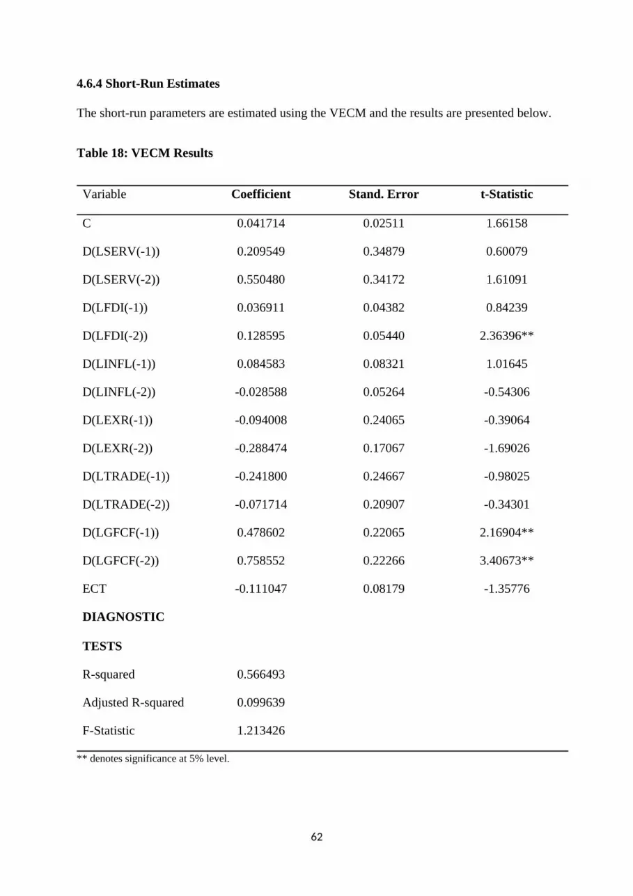
4.6.4 Short-Run Estimates

The short-run parameters are estimated using the VECM and the results are presented below.

Table 18: VECM Results

Variable Coefficient Stand. Error t-Statistic

C 0.041714 0.02511 1.66158

D(LSERV(-1)) 0.209549 0.34879 0.60079

D(LSERV(-2)) 0.550480 0.34172 1.61091

D(LFDI(-1)) 0.036911 0.04382 0.84239

D(LFDI(-2)) 0.128595 0.05440 2.36396**

D(LINFL(-1)) 0.084583 0.08321 1.01645

D(LINFL(-2)) -0.028588 0.05264 -0.54306

D(LEXR(-1)) -0.094008 0.24065 -0.39064

D(LEXR(-2)) -0.288474 0.17067 -1.69026

D(LTRADE(-1)) -0.241800 0.24667 -0.98025

D(LTRADE(-2)) -0.071714 0.20907 -0.34301

D(LGFCF(-1)) 0.478602 0.22065 2.16904**

D(LGFCF(-2)) 0.758552 0.22266 3.40673**

ECT -0.111047 0.08179 -1.35776

DIAGNOSTIC

TESTS

R-squared 0.566493

Adjusted R-squared 0.099639

F-Statistic 1.213426

** denotes significance at 5% level.

62

Results from the short-run estimates show that both the first and second lagged value of FDI

positively affects the service sector. However, only the second lagged coefficient is

significant. In particular, a 1% rise in FDI significantly increases short-run value additions in

the service sector by 0.13%. However, the impact of FDI on the service sector loses its

significance in the long-run. Further results reveal that gross fixed capital formation

positively and significantly impact on the service sector in the short-run. This is true given

the coefficients of its first and second lags. This implies that in the short-run additions to

capital stock improves the service sector. This could take the form of improvement in the

transport systems thus increasing the facilitation role of the service sector. Inflation, trade

openness and exchange rate are not significant drivers of the service sector at least in the

short-run.

4.7 Impact of FDI on the Industrial Sector

4.7.1 VAR Lag Length Selection

As a precondition for the Johansen cointegration test, the lag order selection criteria were

conducted. To minimize information criteria, a lag length of 2 was selected based on the

Schwarz information criterion. Various information criteria suggested lag lengths and these

are shown in Table 19 below:

63

Table 19: VAR Lag Order Selection Criteria on the impact of FDI on the industrial

sector

Endogenous variables: LINDUS LFDI LINFL LEXR

LTRADE LGFCF 

Exogenous variables: C 

 Lag LogL LR FPE AIC SC HQ

0  78.08444 NA   2.34e-10 -5.148889 -4.863416 -5.061617

1  209.6566   197.3583*  2.71e-13 -11.97547  -9.977166* -11.36457

2  251.0296  44.32821  2.74e-13 -12.35926 -8.648117 -11.22473

3  309.3834  37.51317   2.06e-13*  -13.95596* -8.531984  -12.29780*

 * indicates lag order selected by the criterion

 LR: sequential modified LR test statistic (each test at 5% level)

 FPE: Final prediction error

 AIC: Akaike information criterion

 SC: Schwarz information criterion

 HQ: Hannan-Quinn information criterion

64

4.7.2 Johansen Cointegration Test

Table 20: Unrestricted Cointegration Rank Test (Trace)

Series: LINDUS LFDI LINFL LEXR LTRADE LGFCF 

Lags interval (in first differences): 1 to 2

Hypothesized Trace 0.05

No. of CE(s) Eigenvalue Statistic Critical Value Prob.**

None *  0.891540  158.1785  95.75366  0.0000

At most 1 *  0.742053  95.98002  69.81889  0.0001

At most 2 *  0.675680  58.03996  47.85613  0.0042

At most 3  0.478013  26.51131  29.79707  0.1141

At most 4  0.255256  8.308164  15.49471  0.4330

At most 5  0.002003  0.056140  3.841466  0.8127

 Trace test indicates 3 cointegratingeqn(s) at the 0.05 level

 * denotes rejection of the hypothesis at the 0.05 level

 **MacKinnon-Haug-Michelis (1999) p-values

65

Table 21: Unrestricted Cointegration Rank Test (Maximum Eigenvalue)

Hypothesized Max-Eigen 0.05

No. of CE(s) Eigenvalue Statistic Critical Value Prob.**

None *  0.891540  62.19845  40.07757  0.0000

At most 1 *  0.742053  37.94006  33.87687  0.0155

At most 2 *  0.675680  31.52865  27.58434  0.0147

At most 3  0.478013  18.20315  21.13162  0.1224

At most 4  0.255256  8.252024  14.26460  0.3537

At most 5  0.002003  0.056140  3.841466  0.8127

 Max-eigenvalue test indicates 3 cointegratingeqn(s) at the 0.05 level

 * denotes rejection of the hypothesis at the 0.05 level

 **MacKinnon-Haug-Michelis (1999) p-values

Table 20 and 21 show results of the Johansen cointegration test based on the trace and

maximum-eigenvalue test statistics respectively. From the Tables above, both test statistics

reject the null hypothesis of no cointegration. Rejecting the null hypothesis suggest the

existence of cointegration among the variables. Interestingly, each test statistic suggests 3

cointegrating equations and hence a long-run relationship between the industrial sector and

our independent variables including FDI.

4.7.3 Long-Run Estimates

Since the Johansen cointegration test shows a long-run relationship between the industrial

sector and the independent variables including FDI, we estimate the long-run impact of FDI

on the industrial sector while controlling for the independent variables influencing the sector.

Table 22 presents the results of the estimation.

66

Table 22: Long-Run Impact of FDI on the Industrial Sector

Dependent Variable: LINDUS

Variable Coefficient Std. Error t-Statistic Prob.  

C 0.750272 0.243777 3.077697 0.0050

LFDI 0.121213 0.022418 5.946230 0.0001*

LINFL -0.036627 0.044916 -0.815466 0.4225

LEXR -0.124662 0.022937 -5.434972 0.0000*

LTRADE 0.508073 0.129446 3.924970 0.0006*

LGFCF 0.512411 0.164560 3.113824 0.0046*

Diagnostic Tests

R-squared 0.952279    

Adjusted R-squared

F-statistic

0.942735

99.77656    

Prob(F-statistic)

Durbin Watson stat

Serial Correlation LM Test (p-value)

Normality: Jarque-Bera test (p-value)

Heteroskedasticity: Chi-square (p-value)

0.000000

1.243594

5.869305

0.887254

2.303311

(0.0531)

(0.641705)

(0.8058)

Note: * denotes significance at 1% level. Standard errors are White Heteroskedasticity-Consistent.

The diagnostic checks results show that about 94% of the variation in the industrial sector is

determined by variations in our independent variables after accounting for the degrees of

67

freedom. The value of the F-statistic shows the overall significance of the variables. Further

results show that our model passes all the diagnostic test of residual serial correlation,

normality and heteroskedasticity. The results show that FDI positively and significantly

impact the industrial sector. In particular, a 1% increase in FDI inflows increases industrial

value additions by 0.12%. This impact is significant at conventional levels. This is not

surprising because FDI stimulates local investment by raising domestic investment through

links in the production chain as well as facilitating enhanced technology transfer. The

coefficient of exchange rate is negative and significant. Specifically, a rise in the exchange

rate reduces the value additions of the industrial sector by 0.12%. An increase in the

exchange rate implies depreciation of the Cedi and to the extent that this happens, price of

imported inputs rise hence lower demand for inputs and consequently lower production as

cost of production rises. This undoubtedly adversely affects the sector’s value additions.

The coefficient of trade openness is positive and significant at 1% level where a unit-

percentage increase in trade openness increases the long-run value additions of industrial

sector by 0.51%. This effect is expected since Ghana’s involvement in international trade

permits the sector to import foreign capital machinery and equipment necessary to increase

output. Further results show that capital formation positively and significantly drives

industrial output. Specifically, an increase in gross fixed capital formation by 1%

significantly increases industrial value additions by 0.51%. This result is expected given the

role of capital stock in propelling industrial production.

68

4.7.4Short-Run Estimates on impact of FDI on the industrial sector

Results from the VECM which show the short-run impact of FDI on the industrial sector are

presented in Table 23 below.

Table 23: VECM Results

Variable Coefficient Stand. Error t-Statistic

C -0.030062 0.04093 -0.73452

D(LINDUS(-1)) 0.406025 0.38740 1.04809

D(LINDUS(-2)) -0.078040 0.39442 -0.19786

D(LFDI(-1)) 0.016280 0.07126 0.22846

D(LFDI(-2)) 0.083857 0.07444 1.12647

D(LINFL(-1)) -0.161946 0.09189 -1.76240

D(LINFL(-2)) -0.042529 0.05742 -0.74071

D(LEXR(-1)) 0.511152 0.23250 2.19850**

D(LEXR(-2)) 0.168643 0.25775 0.65429

D(LTRADE(-1)) -0.040386 0.31114 -0.12980

D(LTRADE(-2)) 0.121086 0.26849 0.45098

D(LGFCF(-1)) 0.388253 0.28286 1.37262

D(LGFCF(-2)) 0.273286 0.31455 0.86880

ECT -0.045325 0.04437 -1.02149

DIAGNOSTIC

TESTS

R-squared 0.693906

Adjusted R-squared 0.364265

F-Statistic 2.105039

Notes: ** denotes 5% significance level.

69

From the Table above, although the coefficient of the error term meets the expected sign, it is

insignificant suggesting that short-run deviations may not fully return to long-run equilibrium

following a system shock. Both the first and second lag coefficient of FDI are positive

implying that in the short-run, FDI inflows positively to affects the industrial sector.

However, this effect is insignificant at conventional levels. This finding is consistent with the

long-run effect only in terms of the direction of effect and inconsistent in terms of the level of

significance. This means that FDI has no significant impact on the industrial sector in the

short-run but only becomes significant in the long-run.

Further results show the insignificance of the effect of inflation on the industrial sector

although its coefficient is negative. This finding is akin to its long-run impact both in

direction of effect and insignificance. This means that irrespective of the time period,

inflation has no significant impact on the sector.

The coefficients of gross fixed capital formation are positive implying that a rise in capital

formation increases value additions of the industrial sector. However, this effect is only

imaginary in the short-run. Our long-run analysis earlier revealed a positive and significant

effect of capital formation on this sector. This finding suggests that building capital stock

does not have any significant short-run impact on this sector perhaps the capital stock might

not have been into its full utilization.

While the coefficients of exchange rate are positive, only the first lag coefficient is

significant. In particular, a unit-percentage increase in exchange rate increases the short-run

industrial value additions by 0.51%. The implication is that depreciation of the exchange rate

increases the exports as the prices of our exports are cheaper hence higher demand. The

increase in exports could perhaps increase the short-run production levels.

70

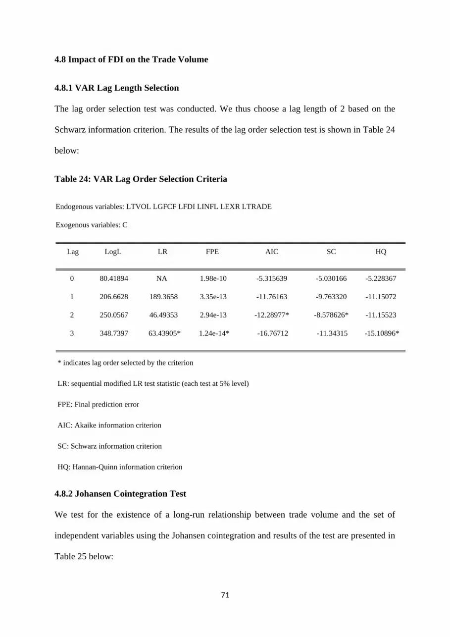
4.8 Impact of FDI on the Trade Volume

4.8.1 VAR Lag Length Selection

The lag order selection test was conducted. We thus choose a lag length of 2 based on the

Schwarz information criterion. The results of the lag order selection test is shown in Table 24

below:

Table 24: VAR Lag Order Selection Criteria

Endogenous variables: LTVOL LGFCF LFDI LINFL LEXR LTRADE 

Exogenous variables: C 

 Lag LogL LR FPE AIC SC HQ

0  80.41894 NA   1.98e-10 -5.315639 -5.030166 -5.228367

1  206.6628  189.3658  3.35e-13 -11.76163 -9.763320 -11.15072

2  250.0567  46.49353  2.94e-13 -12.28977* -8.578626* -11.15523

3  348.7397   63.43905*   1.24e-14*  -16.76712  -11.34315  -15.10896*

 * indicates lag order selected by the criterion

 LR: sequential modified LR test statistic (each test at 5% level)

 FPE: Final prediction error

 AIC: Akaike information criterion

 SC: Schwarz information criterion

 HQ: Hannan-Quinn information criterion

4.8.2 Johansen Cointegration Test

We test for the existence of a long-run relationship between trade volume and the set of

independent variables using the Johansen cointegration and results of the test are presented in

Table 25 below:

71

Table 25: Unrestricted Cointegration Rank Test (Trace)

Series: LTVOL LGFCF LFDI LINFL LEXR LTRADE 

Hypothesized Trace 0.05

No. of CE(s) Eigenvalue Statistic Critical Value Prob.**

None *  0.943299  187.2495  95.75366  0.0000

At most 1 *  0.847650  106.8905  69.81889  0.0000

At most 2 *  0.662872  54.20632  47.85613  0.0113

At most 3  0.376343  23.76216  29.79707  0.2107

At most 4  0.240292  10.54185  15.49471  0.2413

At most 5  0.096676  2.846867  3.841466  0.0915

 Trace test indicates 3 cointegratingeqn(s) at the 0.05 level

 * denotes rejection of the hypothesis at the 0.05 level

 **MacKinnon-Haug-Michelis (1999) p-values

72

Table 26: Unrestricted Cointegration Rank Test (Maximum Eigenvalue)

Hypothesized Max-Eigen 0.05

No. of CE(s) Eigenvalue Statistic Critical Value Prob.**

None *  0.943299  80.35905  40.07757  0.0000

At most 1 *  0.847650  52.68417  33.87687  0.0001

At most 2 *  0.662872  30.44416  27.58434  0.0209

At most 3  0.376343  13.22031  21.13162  0.4322

At most 4  0.240292  7.694981  14.26460  0.4106

At most 5  0.096676  2.846867  3.841466  0.0915

 Max-eigenvalue test indicates 3 cointegratingeqn(s) at the 0.05 level

 * denotes rejection of the hypothesis at the 0.05 level

 **MacKinnon-Haug-Michelis (1999) p-values

Tables 25 and 26 show the results of the Johansen cointegration test based on the trace and

maximum-eigenvalue respectively. Both test statistics reject the null hypothesis of no

cointegration and suggests three cointegrating equations. This confirms the existence of a

long-run relationship among the variables. We thus estimate the long-run parameters and

results are presented in Table 27.

4.8.3 Long –Run Estimates

This section discusses the long-run impact of FDI on trade volumes. Diagnostic results from

Table 27 show the overall significance of the independent variables. This is seen in the high

F-statistic (16.19401) and low p-value (0.0000). Further results show that our model passes

all the diagnostic test of residual serial correlation, normality and heteroskedasticity. Our

findings reveal a positive and significant long-run impact of FDI on trade volume where a

unit percentage increase in FDI significantly (at 1% level) increases trade volumes by

73

0.103%. Thus, the inflows of FDI boost the level of domestic economic activities and trade

volumes in the country. This finding is consistent with SeilanandJayachandran (2013) who

also found a direct relationship between FDI and trade volumes in India.

Table 27: Long-run Impact of FDI on Trade Volume

Dependent Variable: LTVOL

Variable Coefficient Std. Error t-Statistic Prob.  

C 0.339564 0.15948 2.12921 0.0000

LFDI 0.103168 0.01313 7.85464 0.0000*

LINFL -0.061119 0.050041 -1.22138 0.5251

LEXR -0.230276 0.13488 -1.70729 0.0401*

LTRADE 0.064508 0.03270 1.97280 0.0130**

LGFCF 0.080934 0.03214 2.51833 0.0403**

Diagnostic Tests

R-squared 0.914985    

Adjusted R-squared

F-statistic

0.892871

16.19401    

Prob(F-statistic)

Durbin Watson stat

Serial Correlation LM Test (p-value)

Normality: Jarque-Bera test (p-value)

Heteroskedasticity: Chi-square (p-value)

0.00000

1.69125

4.71641

0.48317

5.89432

(0.4365)

(0.6421)

(0.2144)

Notes: * (**) denote significance at 1% (5%) significant level. Standard errors are WhiteHeteroskedasticity-

Consistent Standard Errors and Covariance

74

Turning to the control variables, the coefficient of inflation is negative implying where a unit

rise in consumer price index decreases trade volume by 0.06 units given its coefficient.

However, this effect is insignificant. Further results also reveal an inverse long-run

relationship between exchange rate and trade volume. Specifically, a 1% depreciation of the

Cedi significantly decreases trade volumes by 0.23%. This means that exchange rate

volatility and depreciation in particular hurts trade volumes as more domestic currency –

Ghana Cedi – would be needed to get a unit of foreign currency (say Dollar) in order to trade

with other foreign partners.

The impact of trade openness on trade volume is positive and significant at conventional

levels. Its coefficient is 0.064 implying that a 1% rise in trade openness increases long-run

trade by 0.064%. The implication is that the opening up of Ghana’s trade with trading

partners permits the influx of capital necessary for propelling domestic trade. The coefficient

of capital formation is positive and significant suggesting that increase in capital stock is

good for trade as the existence of crucial infrastructure like roads and capital equipment

facilitates trading.

4.8.4 Short–Run Estimates

While the analysis above shows the long-run impact of FDI on trade volumes. We investigate

the short-run effects of FDI on trade volumes by controlling for factors namely inflation,

exchange rate, gross fixed capital formation and trade openness. Results from the VECM are

shown in Table 28 below:

75

Table 28: VECM Results

Variable Coefficient Stand. Error t-statistic

C 0.016966 0.00701 2.41873

D(LTVOL(-1)) 0.554654 1.29447 0.42848

D(LTVOL(-2)) 1.628749 1.41403 1.15184

D(LGFCF(-1)) 0.139344 0.19855 0.70181

D(LGFCF(-2)) 0.059181 0.22353 0.26476

D(LFDI(-1)) 0.008590 0.00823 1.04418

D(LFDI(-2)) 0.011459 0.00647 1.77062

D(LINFL(-1)) -0.007799 0.00910 -0.85727

D(LINFL(-2)) -0.007254 0.00586 -1.23855

D(LEXR(-1)) 0.014077 0.03040 0.46306

D(LEXR(-2)) -0.039221 0.02507 -1.56458

D(LTRADE(-1)) 1.683010 0.27014 6.23015**

D(LTRADE(-2)) 1.804917 0.34891 5.17297**

ECT -0.017003 0.00544 -3.12297**

DIAGNOSTIC

TESTS

R-squared 0.675354

Adjusted R-squared 0.426162

F-Statistic 4.652953

Notes: ** denotes significance at 5% level.

The initial conditions of the trade volume as denoted by its lagged coefficients are positive

and insignificant. Both the first and second lag coefficients of FDI are positive suggesting

that in the short–run an increase in FDI increases trade. However, this effect is less

76

significant. While the short-run effect of FDI on trade volume is insignificant, it gains

significance in the long-run.

Turning to the control variables, the short-run coefficients of inflation are both negative

implying that increases in inflation retards trade volume. However, both the first and second

lags are insignificant suggesting that at least in the short-run, inflation does not affect trade

volume. Although both the first and second lag coefficients of exchange rate have varying

signs, they are insignificant. This implies that, while exchange rate significantly influences

trade volumes in the long-run, its effect in the short-run is only imaginary. However, the

effect of trade openness is positive and significant given the t-statistics of the first and second

lags coefficients. Thus, in the short-run only, trade openness affects trade volumes.

Conclusively, trade openness enhances trade both in the short- and long-run.

The coefficient of the error correction term is consistent with the theoretical expectation –

negative and significant – and shows a sluggish return to long-run equilibrium following a

shock to the system.

4.9 Conclusion

In addition to assessing the impact of FDI on economic growth, the aim of this chapter was to

present an analysis of impact of FDI on the various sectors of the economy as well as drivers

of trade openness. Relying on annual data spanning 1980 to 2013 and employing Johansen

cointegration and vector error correction model (VECM), the study found a positive and

significant impact of FDI on economic growth. At the sectoral level, while its effect on the

agric sector is negative, FDI inflows positively affect the value additions of the industrial

sector. Its impact on the service sector is however less significant. Further results show that

while inflation is not a significant determinant of trade volume. This is true both in the short-

77

and long-run. In the long-run,while FDI, capital formation and trade openness positively

affects trade volume, depreciation of the Cedi depresses trade volumes.

78

CHAPTER FIVE

FINDINGS, CONCLUSION AND RECOMMENDATIONS

5.1 Introduction

Under This chapter, the study is divided into three (3) sections. The first part deals with a

summary of the major findings of the study. Whiles the second part concludes the study while

the last section presents some recommendations for policy. While the summary presents a

brief overview of the objectives, methodology and findings, the conclusion presents the

overall outcomes of the study. Recommendations however, provide some policy prescriptions

to increasing FDI inflows in Ghana as well improve its impact on various sectors of the

economy.

5.2 Summary

Apart from assessing the impact of FDI on the economy performance in Ghana, the study

also considered the effects of FDI on the various sectors of the economy as well as the

contribution of Foreign Direct Investment to trade openness. This was done relying on annual

data gleaned from different sources spanning 1980 to 2013. The work adopted Johansen

(1988) methods to cointegration and the VECM to determine the long-run and short-run

behaviours amongst the variables used in the estimation. The variables employed in the study

included FDI express as a percentage of GDI, gross fixed capital formation, inflation, trade

openness, exchange rate, trade volume, service , agriculture and industrial sectors as the share

of GDP. To correct for heteroskedasticity, all variables in the long-period were estimated

while reporting White’s (1980) heteroskedasticity–consistent standard errors. Results from all

the cointegration tests showed the existence of at least one cointegrating equation hence long-

run relationships.

79

The study revealed that Foreign Direct Investment positively and significantly influence real

GDP. This is true irrespective of the time period. While depreciation of the Cedi positively

affects long-period real GDP growth, its short-time effect is only imaginary. Inflation

negatively impact on fiscal development but this effect is more pronounced only in the short-

time.

On the drivers of the value additions of the agric sector, Foreign Direct Investment negatively

affects the long-run performance of this sector although its short-period impact is positive.

Depreciation of the currency also adversely affects this sector perhaps owing to higher cost of

imported capital. Although trade openness has no significant impact on the agriculture sector

in the short-time, an increase in trade openness significantly raises the long-run value

additions of this sector.

Further results show that Foreign Direct Investment has no significant on long-period value

additions of the service sector. However, in the short-run only its second lag coefficient is

positive and significant. It is observed that in the long-run, only exchange rate and trade

openness drive the service sector where an increase in any of these metrics significantly

raises the value additions of the service sector. In the short-run, while gross fixed capital

formation positively influence service sector, trade openness and exchange rate do not affect

the sector’s value additions.

The long-period impact of Foreign Direct Investment on the industrial sector is positive and

significant. Also important positive drivers of industrial value additions in the long-run are

gross fixed capital formation and trade openness. It is observed that on the short-term,

depreciation of the currency improves the industrial sector. However, depreciation of the

Cedi hurts the sector’s long-run value additions. While Foreign Direct Investment, trade

openness and capital formations do not affect the short-run industrial value additions,

80

inflation on the other hand has no impact on the industrial sector whether we are in the short-

or long-run.

Also observed from the study is that, in the long-period, Foreign Direct Investment, capital

formation and trade openness affect trade volumes and an increase in any of these increase

the volume of trade. The effect of exchange rate is however negative. However, in the short-

run only trade openness drive the amount of trade volume.

5.3 Conclusion

The impact of FDI in economic, fiscal growth and development cannot be overemphasized.

Foreign Direct Investment is seen as the most significant supply of external resource flows to

many African nations with investible resources to finance long-term investment. However,

empirical literature on the role of Foreign Direct Investment on growth has been mixed and

inconclusive necessitating further research effort. In addition, sectoral impact of FDI as well

as drivers of trade volume has been relatively understudied.

In line with the empirical literature, the study concludes a positive long-run connection

between real GDP and the set of independent variables including FDI. Our results suggest

that FDI inflows significantly improves real GDP hence the Ghanaian economy. At the

sectoral level, it can further be concluded that while FDI has no impact on the service sector,

it however exerts a negative effect on the agric sector. Nonetheless, the inflows positively and

significantly increase the value additions of the industrial sector and trade volume more

generally.

5.4 Recommendations

By taking cognizance of the findings, this study seeks to make a number of

recommendations.

81

The study found a positive long-run connection between Foreign Direct Investment and

economic growth and development which is an indication that inflows of Foreign Direct

Investment play a critical task in growth of the economy. In respect of this, government with

the Bank of Ghana, Ministry of Trade and Industry, and other stakeholders should deepen and

maintain a continued trade relations with the rest of the world in order to attract FDI which

promotes economic growth.

Again, executive and other arms of government must be committed to deepen the democratic

path that the nation chose as means of electing our leaders. As stable democracy can be

attracting factor to FDI inflows. Government must ensure Stable microeconomics and

macroeconomics conditions in the country.

In addition to revealing a negative relationship between FDI and the agric sector, the

empirical evidence showed no adjustment to equilibrium from the short-run and this was

attributed to the presence of constraints in the sector hence forcing people to seek

opportunities in other sectors. As such, there is the need for the government to ensure that

constraints such as inadequate road network, low commodity prices at the international

market and lack of credit to farmers are eliminated in order to increase productivity so that a

self-sustained value addition could take place.

The study found trade openness as a powerful tool to increasing the value additions of all the

sectors and hence economic growth. As such, it is imperative for government to continue

liberalizing our domestic markets in order to attract various forms of capital necessary for

propelling growth.

82

REFERENCES

Abel, E.E. and Nikki, C. (2011). FDI flows to Sub-Saharan Africa: the impact of

finance,institution and natural eendowment, Department of Economics and Economic

History, Rhodes University, Grahams town, South Africa

Adam,A.M and Tweneboah,G., (2008a). Do macroeconomic variables play any role in the

stock market movement in Ghana? MPRA Paper [online]. Available at:http//mpra.ub.uni-

muenechen.de/9301/

Adam,A.M and Tweneboah,G., (2008b). Foreign Direct Investment (FDI) And stock Market

Development: Ghana Evidence MPRA Paper [online]. Available at:http//mpra.ub.uni-

muenechen.de/11264/

Asafu-Adjaye, J (2005), “What has been the impact of Foreign Direct Investment in Ghana?”

IEA Policy Analysis, Vol. 1 No. 9 ISSN 08552452

Barthel, F., Busse, M, and Osei,R. (2008). The Characteristics and Determinants of FDI in

Ghana. HWWI Research Papr, No.2-15

Basu, P.; Chakraborty, C.; and Reagle, D. (2003). Liberalization, FDI and Growth in

Carkovic, M; Levine, R. (2002, August 28). Does foreign direct investment accelerate

economic growth? University of Minnesota Department of Finance working Paper.

Carkovic, M; Levine,R. (2002). Does foreign direct investment accelerate economic growth?

University of Minnesota Department of Finance working Paper.

Caves, R. (1971). International Corporations: The industrial economics of foreign investment,

Economica, 38(149) , 1-27

Cointegration with Application to the Demand for Money.Oxford Bulletin of Economics

Dunning, J. H . (1988). "Explaining International Production", Unwin Hyman: London,

83

Dunning, J. H. (1981). "International Production and the Multinational Enterprise", Allen and

Unwin: London.

Dunning, J. H. (1992). "Multinational Enterprises and the Global Economy", Addison

Wesley: London.

Dunning, J. H. (2001). “The Eclectic (OLI) Paradigm of International Production: Past,

Present and Future,” International Journal of the Economics of Business, 8(2), 173-190.

Dynamics and Control, 12(2-3), 231–254.

Frimpong, J. M., and Oteng-Abayie, E. F., (2008). Bivariate Causality Analysis between FDI

Inflows and Economic Growth in Ghana, International Research Journal of Finance and

Economics, 15: 103 – 112.

Funke N, Nsouli SM (2003). The New Partnership for Africa’s Development (NEPAD):

Opportunities andChallenges. IMF, Washington, DC. IMF Working paper No. 03/69.

Garba, S. T. Direct Private Foreign Investment and Economic Growth in Nigeria (1980-

1996): An Empirical Investigation [D]. (Unpublished Ph.D. Thesis) submitted to the

Postgraduate School, ABU, Zaria. 1998

Herzer, D., Klasen, S. and Nowak-Lehmann, D.F. (2006). In search of FDI-led growth in

developing countries: The way forward”. Ibero American Institute for Economic Research

http://dx.doi.org/10.1016/0165-1889(88)90041-3

Ibrahim, A. 2005),“ Sectoral Analysis of Foreign Direct Investment in Ghana”, BOG research

paper, ResearchDepartment, Bank of Ghana

Johansen, S. (1988).Statistical Analysis of CointegrationVectors.Journal of Economic

Johansen, S. (1991). Estimation and Hypothesis testing of Cointegration Vector in Gaussian

Johansen, S., &Juselius, K. (1990). Maximum Likelihood Estimation and Inference on

84

Karikari, J. A. (1992). Causality between Direct Foreign Investment and Economic Output in

Ghana.JournalofEconomic Development 17 (1), 7-17. Accessed and downloaded from

http://www.jed.or.kr/full-text/17-1/1.pdf on 9thJune 2011 at 11:19 GMT

Maximum Likelihood Cointegration Rank Test Statistics: Four Cases. Oxford Bulletin of

McCloud, N. and Kumbhakar, S. C. (2011). Institutions, foreign direct investment and

growth: a hierarchical Bayesian approach. Journal of the Royal Statistical Society: Series A

(Statistics in Society). http://dx.doi.org/10.1111/j.1467-985X.2011.00710.x

Osterwald-Lenum, M. (1992). A Note with Fractiles of the Asymptotic Distribution of the

Samimi, A. J., ZeinabRezanejad and FaezehAriani (2010), “Growth and FDI in OIC

Countries” Australian Journal of Basic and Applied Sciences, 4(10): 4883-4885

Vector Autoregressive Models.Econometrica, 59(6), 1551-1581.

http://dx.doi.org/10.2307/2938278

UNCTAD (2002). World Investment Report 2002. Geneva: UNCTAD

UNCTAD (2005): “Economic Development In Africa: Rethinking The of Foreign Direct

Investment”,

Wilhems. S.K.S., (1998): foreign direct investment and its determinants in emerging

economies. Africa Economic Policy policy paer No. 9.

http://www.eagerproject.com/discussion9.shtml.

World Bank (2013), World Development Indicators online database, Washington DC.

Zhang, K. H. (2001), “How Does Foreign Direct Investment Affect Economic Growth?”

Economic of transition, 9(3), 679-693

85

APPENDIX

Heteroskedasticity Test: Breusch-Pagan-Godfrey

F-statistic 4.234014    Prob. F(5,25) 0.0063

Obs*R-squared 14.21423    Prob. Chi-Square(5) 0.0143

Scaled explained SS 13.22812    Prob. Chi-Square(5) 0.0213

Breusch-Godfrey Serial Correlation LM Test:

F-statistic 3.489696    Prob. F(2,23) 0.0475

Obs*R-squared 7.216996    Prob. Chi-Square(2) 0.0271

 Unrestricted Cointegrating Coefficients (normalized by b'*S11*b=I): 

LRGDP LFDI LINFL LEXR LTRADE LGFCF

 11.60061 -9.109068  7.826963  6.822464 -16.51893  20.40055

-109.4877  9.517677 -0.610987  25.34211 -33.49707 -34.97192

 10.54738 -2.654307 -4.263889 -1.154025 -17.57263  29.42789

-67.19785  4.377389 -11.24700  15.20702 -15.07640 -19.25236

 0.006598 -3.251710 -2.603255  3.506621 -8.918563  0.270745

 18.28389  1.159947  5.753796 -0.443892  8.158118 -18.51496

 Unrestricted Adjustment Coefficients (alpha): 

D(LRGDP)  0.003921 -0.000744  0.001252  0.000243  0.001083

D(LFDI)  0.038479  0.012266  0.000967 -0.025246  0.059287

D(LINFL) -0.108905 -0.034631 -0.014385  0.056891  0.008193

D(LEXR) -0.038491  0.002121  0.001142 -0.004317  0.015529

D(LTRADE) -0.017429  0.029513  0.006491  0.001193  0.005980

D(LGFCF)  0.016422  0.020657 -0.021833  0.008340  0.015062

86

1 Cointegrating Equation(s):  Log likelihood  314.9396

Normalized cointegrating coefficients (standard error in parentheses)

LRGDP LFDI LINFL LEXR LTRADE LGFCF

 1.000000 -0.785223  0.674703  0.588113 -1.423971  1.758575

 (0.07593)  (0.11124)  (0.08679)  (0.24388)  (0.31767)

Adjustment coefficients (standard error in parentheses)

D(LRGDP)  0.045482

 (0.01051)

D(LFDI)  0.446381

 (0.58688)

D(LINFL) -1.263370

 (0.36190)

D(LEXR) -0.446519

 (0.11687)

D(LTRADE) -0.202187

 (0.12396)

D(LGFCF)  0.190508

 (0.16887)

2 Cointegrating Equation(s):  Log likelihood  333.1278

Normalized cointegrating coefficients (standard error in parentheses)

LRGDP LFDI LINFL LEXR LTRADE LGFCF

 1.000000  0.000000 -0.077717 -0.333488  0.521297  0.140256

 (0.02679)  (0.01294)  (0.03553)  (0.05687)

 0.000000  1.000000 -0.958224 -1.173680  2.477344 -2.060968

87

 (0.16059)  (0.07755)  (0.21296)  (0.34087)

Adjustment coefficients (standard error in parentheses)

D(LRGDP)  0.126993 -0.042799

 (0.09736)  (0.01165)

D(LFDI) -0.896645 -0.233761

 (5.55831)  (0.66509)

D(LINFL)  2.528247  0.662425

 (3.28013)  (0.39249)

D(LEXR) -0.678783  0.370808

 (1.10743)  (0.13251)

D(LTRADE) -3.433527  0.439660

 (0.79367)  (0.09497)

D(LGFCF) -2.071211  0.047018

 (1.48303)  (0.17745)

3 Cointegrating Equation(s):  Log likelihood  345.1159

Normalized cointegrating coefficients (standard error in parentheses)

LRGDP LFDI LINFL LEXR LTRADE LGFCF

 1.000000  0.000000  0.000000 -0.323728  0.735402 -0.151503

 (0.01826)  (0.06496)  (0.09163)

 0.000000  1.000000  0.000000 -1.053348  5.117170 -5.658250

 (0.19335)  (0.68785)  (0.97027)

 0.000000  0.000000  1.000000  0.125578  2.754914 -3.754113

 (0.19667)  (0.69964)  (0.98690)

Adjustment coefficients (standard error in parentheses)

D(LRGDP)  0.140195 -0.046121  0.025804

88

 (0.09053)  (0.01100)  (0.00731)

D(LFDI) -0.886446 -0.236327  0.289557

 (5.58368)  (0.67844)  (0.45101)

D(LINFL)  2.376523  0.700607 -0.769904

 (3.26760)  (0.39703)  (0.26394)

D(LEXR) -0.666737  0.367777 -0.307434

 (1.11199)  (0.13511)  (0.08982)

D(LTRADE) -3.365068  0.422431 -0.182124

 (0.77388)  (0.09403)  (0.06251)

D(LGFCF) -2.301491  0.104969  0.209008

 (1.34277)  (0.16315)  (0.10846)

4 Cointegrating Equation(s):  Log likelihood  351.4986

Normalized cointegrating coefficients (standard error in parentheses)

LRGDP LFDI LINFL LEXR LTRADE LGFCF

 1.000000  0.000000  0.000000  0.000000 -25.80777  28.84130

 (6.47659)  (8.10319)

 0.000000  1.000000  0.000000  0.000000 -81.24908  88.67860

 (20.7179)  (25.9212)

 0.000000  0.000000  1.000000  0.000000  13.05130 -15.00074

 (3.09374)  (3.87074)

 0.000000  0.000000  0.000000  1.000000 -81.99214  89.55906

 (20.1517)  (25.2128)

Breusch-Godfrey Serial Correlation LM Test:

F-statistic 1.211014    Prob. F(2,24) 0.3155

Obs*R-squared 2.841676    Prob. Chi-Square(2) 0.2415

89

Heteroskedasticity Test: Breusch-Pagan-Godfrey

F-statistic 0.620572    Prob. F(4,26) 0.6519

Obs*R-squared 2.701711    Prob. Chi-Square(4) 0.6089

Scaled explained SS 1.336212    Prob. Chi-Square(4) 0.8552

90