The Jacobi constant for a cometary orbiter

A&A 443, 691–701 (2005)DOI: 10.1051/0004-6361:20053416c© ESO 2005

Astronomy&

Astrophysics

The Jacobi constant for a cometary orbiter

E. Mysen and K. Aksnes

Institute of Theoretical Astrophysics, University of Oslo, PO Box 1029 Blindern, 0315 Oslo, Norwaye-mail: [eirik.mysen;kaare.aksnes]@astro.uio.no

Received 12 May 2005 / Accepted 29 July 2005

ABSTRACT

The Jacobi constant of a probe under the gravitational attraction of a rotating irregular body is rederived for excited, but free rigid rotation ofthe central mass. A related Tisserand-like quantity is found to be sufficiently conserved for it to qualify as a pseudo-integral. The quantity’snear constancy is shown to imply that certain regions in the space of the probe’s cometocentric orbital elements are forbidden. In particular,based solely on this analysis, it is seen how collision with the comet nucleus is best avoided if the initial probe velocity lies in the plane normalto the nucleus’ rotational spin. A conclusion which is of relevance to the Rosetta mission where the lander Philae is to be delivered by Rosettain a possibly close prograde, and therefore probably shape unstable, orbit. At the comet’s heliocentric distance when the lander is delivered,radiation and radial outgassing pressure do not significantly affect these conclusions for a nominal target nucleus in a worst-case scenario. Thelatter effect is seen to somewhat decrease the impact risk of prograde trajectories, making the more stable retrograde orbits slightly less safe.

Key words. celestial mechanics – space vehicles – comets: general – comets: individual: 67P/Churyumov-Gerasimenko – methods: analytical– methods: numerical

1. Introduction

It is well known that close orbits around small irregular celes-tial bodies can experience gravitationally induced rapid, ape-riodic variations in orbital energy. These changes occur atorbital distances and eccentricities for which the resonancesbetween the nucleus spin and the orbiting probe’s orbit havefused, forming a chaotic zone, no longer confined to the sep-aratrices of the resonances, in which the actions of the sys-tem can wander (Lichtenberg & Lieberman 1992). However,if the central body is rotating uniformly, there exists an in-tegral, the Jacobi constant, constraining the probe’s motion.Usually, these constraints are represented geometrically as so-called zero-velocity curves.

As witnessed for 1P/Halley by ESA’s Giotto, the rotationof cometary nuclei could be excited. Therefore, in anticipationof cometary missions like Rosetta, the variation of the Jacobifunction for a spacecraft in an orbit around a non-uniformly ro-tating central body will be studied. If a related function is foundto be sufficiently conserved, the implications for any initial or-bit will be derived.

Not untypical for short-periodic comets, the Rosetta target67P/Churyumov-Gerasimenko is a relatively small (Lamy et al.2003) low density object (Davidsson & Gutiérrez 2005). Eventhough the isolated analysis of the gravitational problem placesrestrictions on the fast gravitationally induced changes of or-bital energy, the effect of the possibly strong non-gravitational

forces must therefore be taken into account if questions oforbital constraints on longer time-scales are to be raised.

2. The nucleus

The comet nucleus’ gravitational field is modelled using astandard spherical harmonics expansion of the gravitationalpotential (Heiskanen & Moritz 1967)

V1 =µc

r

∞∑

n=2

n∑

m=0

(rc

r

)n

Pnm(sin β)

×[ cnm cos mλ + snm sin mλ]. (1)

Here r is the distance between the probe and the mass centerof the nucleus whose characteristic radius is rc, while λ and βare the spacecraft’s east longitude and north latitude, respec-tively, in the nucleus’ principal axis system (Goldstein 1980).µc is the product of the constant of gravitation and the comet’smass, and Pnm are the Legendre functions. The acceleration ofan orbiting probe induced by gravitation is then

r = −∇(V0 + V1), ∇ =3∑

i=1

uXi

∂

∂Xi, (2)

with the Kepler potential V0 = −µc/r, where Xi = X, Y, Z arethe coordinates in the adopted cometocentric reference system,and uXi are unit vectors defining the reference axes. For conve-nience, the reference XY-plane is assumed to coincide with theplane normal to the nucleus spin Gc.

Article published by EDP Sciences and available at http://www.edpsciences.org/aa or http://dx.doi.org/10.1051/0004-6361:20053416

http://www.edpsciences.org/aa

http://dx.doi.org/10.1051/0004-6361:20053416

692 E. Mysen and K. Aksnes: The Jacobi constant for a cometary orbiter

Jcc

Y

X

x

Plane normal to spin

Mass center

Nucleus equator

g

lc

Fig. 1. The reference system, the principal x-axis and angles of rigidrotation.

In order to calculate the gradient Eq. (2), we have for-mulated V1 in terms of the probe’s Cartesian components Xi.As a first step, observe that each spherical harmonic easily(Heiskanen & Moritz 1967) can be written as a function of theprobe’s Cartesian components xi = x, y, z in the nucleus’ prin-cipal axis system, axes defined by the unit vectors uxi . Theseagain are connected to the spacecraft’s reference system com-ponents X j through a matrix describing the rigid rotation of thecomet

xi =

3∑

j=1

α ji(lc, gc, Jc) X j, αi j = uXi · ux j , (3)

enabling the operation of Eq. (2). Since simulations of 67P’srotation state show that it is possible, although not common,for the rotation to get excited through an orbital run (Gutiérrezet al. 2003), the matrix α must accommodate complex rotation,as indicated by its arguments. As illustrated in Fig. 1, gc is theso-called precession angle, i.e. the node along the plane normalto the spin Gc, of the nucleus’ equator with respect to the ref-erence X-axis. The polhode angle lc is the angular distance ofthe principal x-axis from the spin plane, and is measured alongthe nucleus equator, defined by the principal x- and y-axes. Atlast, Jc is the inclination of the body equator with respect to theplane normal to the comet’s rotational spin. Also according toGutiérrez et al. (2003), torques acting on 67P are negligible forlong periods of time during the Rosetta mission, making thesimulation of the angles above, the two first partially definingthe so-called Andoyer coordinates, very easy. See Kinoshita(1972) for their differential equations. These then appear inEq. (2) as explicit time dependencies. α is straightforward toderive, but can also be found in Beletskii (1966) with the helpof the variable identifications given in Mysen (2004).

For the shape of the comet nucleus the hypothesis ofMuinonen (1998) is adopted where the surface is described bymultivariate normal statistics. The surface correlation angle isset to a low (Muinonen & Lagerros 1998) value Γc = 0.4, i.e.high irregularity, while the standard deviation of the radii is de-fined to be σc = 0.2 rc with rc as the mean radius of the comet.A realization of these parameters is shown in Fig. 2, henceforthadopted as the nucleus.

If we, for simplicity only, define the mass density tobe constant, an assumption which worked well for Eros

Fig. 2. The adopted Gaussian comet nucleus.

(Miller et al. 2002), the coefficients cnm and snm of the expan-sion (1) can be calculated according to (Heiskanen & Moritz1967)

cnm

snm

= γnm

cnm

snm

= −(2 − δ0m)

(n − m)!(n + m)!

×∑

i

mi

mc

(ri

rc

)n Cnm(λi, βi)S nm(λi, βi)

(4)

where

γnm =

√2(2n + 1)(n − m)!(1 + δ0m)(n + m)!

(5)

is a normalization factor so that the square of the normalizedspherical harmonic functions Cnm and S nm

Cnm

S nm

=

1γnm

Cnm

S nm

= Pnm(sin β)

cos mλsin mλ

(6)

equal one when averaged over all directions. δ0m is theKronecker delta. The sum is over all 16601 equidistant, equalpoint masses mi which we have defined the nucleus to consistof. For triaxial ellipsoids with uniform mass density, cnm = 0if n or m odd and snm = 0 (Rossi et al. 1999), making the corre-sponding terms measures of irregularity in our case. However,as long as the body-fixed system is mass centered and alignedwith the principal axes, c21 = s21 = s22 = 0, regardless ofdensity distribution.

Some normalized values are given in Table 1. Since they ingeneral do not vanish with increasing degree, the gravitationalexpansion (1) converges, roughly speaking, outside r ∼ rc

(Garmier & Barriot 2001). The upper row in Table 1 corre-sponds, in this case, to so-called short-axis rotational mode(SAM) of the nucleus, while the lower represents the case ofrotation around the nucleus’ long axis (LAM). ec is the im-portant triaxiality parameter determining the convergence of

E. Mysen and K. Aksnes: The Jacobi constant for a cometary orbiter 693

Table 1. Coefficients of the gravitational field Eq. (1).

ec c20 c22 c30 c32 s33

0.76 0.054 −0.063 −0.0098 −0.0063 −0.0480.075 −0.082 0.015 0.040 0.036 −0.010

Table 2. Nominal 67P characteristics.

mc rc 2πC G−1c

1013 kg 1.98 km 12.3 h

the Andoyer variables’ Fourier expansion in their action-angles(Kinoshita 1972).

Table 2 shows the nucleus mass mc and the other parame-ters which are used in later simulations and can, on the basisof Lamy et al. (2003), Rickman et al. (1987) and Davidsson& Gutiérrez (2005), be considered nominal. C is the momentof inertia along the principal axis of rotation. If the rotation isuniaxial, the nucleus’ rotational velocity ω coincides with thisaxis. For excited rotation,ω circulates around the principal axisof rotation in the nucleus corotating frame. As a consequence,both gc and lc are defined to never librate, but always circulate.The moments of inertia along the two other principal axes ofthe nucleus are A and B. If C is the largest of the three (SAM),we define the order C > B > A. If C is smallest (LAM), thenC < B < A by definition.

3. The Jacobi function

Considering gravitation only, the motion of a probe can be con-strained by a function χ which is an integral for uniaxial rota-tion. Below we shall see to what extent its constancy is violatedin the general rigid body case, also treated in Scheeres et al.(1996).

3.1. Definition

Following Goldstein (1980), the velocity of the probe relativeto the cometocentric, nucleus corotating system is

rb ≡3∑

i=1

uxi xi = r − ω × r, (7)

where ω is the comet’s angular velocity as before. If we takethe time derivative of both sides, and then reapply the originalequation, the relation

rb +ω × rb = r − ω × r −ω × (rb +ω × r) (8)

or

rb ≡3∑

i=1

uxi xi

= r −ω × (ω × r) − 2ω × rb − ω × r, (9)

is obtained. For several important effects, like gravitation, theforce per mass unit f = r is derivable from a potential V

r = f = −∇V ≡ −3∑

i=1

uXi

∂V∂Xi

= −3∑

i, j,k=1

αi j ux j αik∂V∂xk= −

3∑

k=1

uxk

∂V∂xk· (10)

The latter equality follows from the fact that the reference sys-tem and the nucleus corotating system is linked by an orthog-onal transformation, i.e. αT α = 1, see Eq. (3), where T heredenotes the transpose matrix.

The first term of Eq. (9) after r is the centrifugal accelera-tion, derivable from the potential

W = −12

(ω × r)2. (11)

Multiplying both sides of Eq. (9) with rb removes the Corioliscomponent. Furthermore, since the gradient ∇ is a rotationalinvariant, Eq. (10), and the gravitational field is stationary inthe corotating system

rb · ∇V = V , V ≡ V0 + V1. (12)

This is, however, not the case for the centrifugal acceleration

rb · ∇W = W − ∂W∂t= W + (ω × r) · (ω × r). (13)

Defining the Jacobi function as

χ ≡ 12

r2b + V +W, (14)

then yields for its time derivative

χ = −(ω × r) · (rb +ω × r) = −(ω × r) · r. (15)

Using a fundamental vector identity, and the definition of theprobe’s orbital angular momentum G ≡ r × r,

(ω × r) · r = ω · (r × r) ≡ ω · G, (16)

and therefore

χ(t) = χ(t0) − ω · G |tt0 +∫ t

t0

dtω · G (17)

follows for the Jacobi function of a probe in an orbit around acomplex rotating body.

3.2. The modified Jacobi function

Suppose that the probe interacts chaotically with the comet,for instance near its pericenter, altering the spacecraft’s angu-lar momentum with a vector ∆G = G(t) − G(t0). Furthermore,assume that the interaction times tXk

∫ t

t0

dtωXk GXk = ωXk (tXk )∆GXk , t0 < tXk < t, (18)

introduced more for notational convenience, can be defined.Eq. (18) is valid for a wide range of function combinations, but


not as a mathematical statement. For the scenarios which mo-tivate this paper, the orbital angular momentum changes aperi-odically, and Eq. (18) is more true in general. Inserting Eq. (18)into Eq. (17) for several interactions N

G(t) = G(t0) +N∑

i=1

∆Gi, (19)

we obtain

χ(t) − χ(t0) = −N∑

i=1

2∑

j=1

∆GX j ,i [ωX j (t) − ωX j (tX j ,i) ]

−2∑

j=1

GX j (t0) [ωX j(t) − ωX j (t0) ] (20)

by noting that the angular velocity’s component along theZ-axis, ωZ , is constant for a freely rotating rigid body.According to Eq. (20), the Jacobi function deviates from itsepoch value by a series of periodic terms, the last two beingindependent of the orbital evolution.

Without drawing any conclusions yet regarding the termscontaining ∆GX j , it is evident that the parts of Eq. (20) whichare independent of the orbital evolution could be significantfor inclined orbits. However, the components in question canbe removed by converting the comet-fixed probe velocity to itsmore absolute equivalent

χ =12

(r − ω × r)2 − 12

(ω × r)2 + V

=12

r2 + V −ω · G, (21)

which inserted into Eq. (17) with the use of expansions (18),results in

Ω(t) − Ω(t0) =N∑

i=1

2∑

j=1

∆GX j ,i ωX j (tX j ,i), (22)

where the modified Jacobi function is

Ω ≡ 12

r2 + V − ωZ G cos I (23)

with I as the probe orbit’s inclination with respect to the spinplane. If the nucleus rotation is one-axial, then Ω = χ.

3.3. A pseudo-integral

We will now estimate the variations Eq. (22) relative to Ω’spossible range

∆Ω

Ω∼ ωXk (tXk )

ωZ

∆GXk

G, (24)

where it has been assumed that the maximum of the third ofEq. (23)’s terms, and not the two first representing the orbitalenergy, is dominant. That is, we assume that the nucleus is notmuch more massive or much more slowly rotating than ournominal one. However, with the anlysis presented below, esti-mates ofΩ’s absolute change for such cases should be possibleto produce. Following Eq. (24), the conditions for which Ω is

50 100 150 200t h

0.521

0.522

0.523

0.524Ω, ΩM, ΩZ h

1

Fig. 3. The simulated |ω| = √ω2 (variable curve) and ωZ (lower line)are plotted for the nucleus in SAM.ωZ andωM from Eqs. (26) and (27)are also included, but the former is not visible since it concides withits simulated value.

nearly conserved can be found. First consider ωX (tX)/ωZ sincethe analysis for ωY (tY )/ωZ is identical with exactly the samequantitative conclusions.

If one makes the conservative assumption that ωX’s valueat the interaction time is not correlated with ∆GX , the formercan take on all accessible values. These include zero, a mean ω,and a maximum ωm, where the range ωX(tX) ∈ (0, ω) is morerelevant since the chaotic interactions generally take place overtypically a comet rotation period for the nominal parameters.Identifying ω2

m = ω2M − ω2

Z where

ω2M = max[ω2

x + ω2y + ω

2z ], ωZ =

2 Tc

Gc, (25)

with Tc as the nucleus’ rotational kinetic energy, it is straight-forward to derive

ωZ =1ω

2ec + k2(1 − ec)2ec + k2(1 − ec)

(26)

ωM =1ω

√22ec + k2(1 − ec)2ec + k2(1 − ec)

(27)

with the use of the principal axis components ωxk of Kinoshita(1972). Above = A/C, ω = Gc/C, and k is the elliptic mod-ulus of free rotation. For motion on the separatrix separatingthe rotational modes k = 1, while k = 0 means uniaxial rota-tion if B, the intermediary moment of inertia, is not identicalto A, see for instance Hitzl & Breakwell (1971). Based on anumber of simulations of the equations of motion for a freelyrotating rigid body, both Eqs. (26) and (27) have been found tobe correct. Figure 3 shows the results of such a simulation forthe nominal nucleus in SAM at an excited k = 0.500.

The process of obtaining ω is more elaborate. The meanused for its calculation is defined to be

limT→∞

1T

∫ T

0dt =

1(2π)2

∫ 2π

0dlc

∫ 2π

0dgc, (28)

where the equality follows if the rotation is approximatelytorque free. lc is one of the Andoyer action-angles, having aconstant time derivative for free rigid rotation. Actually, theaction-angle gc should also have been used above, but the


integration over the precession angle gc is equivalent since(Kinoshita 1972)

gc = gc +

∞∑

m=1

cm(ec, k) cos 2mlc. (29)

Using the rotation α of Eq. (3), which can be separated into

αi j = α(c)i j cos gc + α

(s)i j sin gc, i 3 (30)

results in

ωX1 = γ(lc) cos gc + δ(lc) sin gc

ωX2 = −δ(lc) cos gc + γ(lc) sin gc, (31)

where, for instance

γ(lc) =3∑

i=1

α(c)1i ωxi , δ(lc) =

3∑

i=1

α(s)1i ωxi , (32)

and therefore

12π

∫ 2π

0dgc ω

2X =

12

(γ2 + δ2). (33)

The remaining integration can be performed after a lengthy,but straightforward formulation of γ2+δ2 in principal axis spincomponents (Kinoshita 1972), which in free rigid body motionare pure functions of lc. Consult Byrd & Friedman (1971) forthe relevant integrals. The end result is

ω ≡√

limT→∞

1T

∫ T

0dtω2

X =1

2√

2ω |1 − 1/| ψ(ec, k) (34)

ψ =2

b(1 + ec)

√(1 + bec)

[ EK

b (1 − ec) + bec − 1]. (35)

where

b(ec, k) =2ec + k2(1 − ec)

ec [ 2 − k2(1 − ec) ], (36)

and K and E are the complete Jacobian elliptic integrals of thefirst and the second kind, respectively

K(k) =∫ π/2

0

dθ√1 − k2 sin2 θ

(37)

E(k) =∫ π/2

0dθ

√1 − k2 sin2 θ. (38)

As for Eqs. (26) and (27), Eq. (34) has been found to be per-fectly consistent with integrals of simulated solutions.

Plotted as Fig. 4 are the ω/ωZ and ωm/ωZ ratios for thenucleus Fig. 2 in SAM (dashed) and LAM (solid). The solidcurve is typical for low triaxial modes, rapidly rising to a largevalue for increasing excitation k. However, it must be stressedthat the lower ec, the higher (the maximum of) Jc must be inorder to produce a specific k. If k is fixed at 0.5, the verticalline of Fig. 4, the iso-contours of the ratio ω/ωZ can be plottedin − ec space, Fig. 5. Clearly, nuclei with high triaxiality, theintermediary moment of inertia B being closer to C than A,

0.2 0.4 0.6 0.8 1k

0.05

0.1

0.15

0.2

ΩΩZ, ΩmΩZ

Fig. 4. ω/ωZ (lower) and ωm/ωZ (upper) as a function of the rotationexcitation parameter k for the low (solid) and high (dashed) triaxialitymode, Table 1.

-1 -0.5 0 0.5 1log10

0

0.2

0.4

0.6

0.8

1ec

0.05 0.05

0.250.25

Fig. 5. Level sets of ω/ωZ in inertia ratio = A/C and triaxialityspace. The values at the curves increase from 0.05 to 0.25 with step0.05 from the center to the left and right. Also included are the ellipsesof Fig. 4, representing the different modes of the nucleus on Fig. 2 atk = 0.5.

which also are elongated, > 1, have small upper boundarieson the relative change of Ω.

As for the second factor of Eq. (24), we begin by observingthat the expansion (1) can be separated into an r = r( f ) and au = f + g dependency for all orders n, with f and g as the trueanomaly of the orbiter and the orbit’s argument of pericenter(Murray & Dermott 1999), respectively. More specifically, forthe n’th harmonics

V (n)1 =

µc

r

(rc

r

)nYn(u), (39)

which yields

G(n) = −∂V (n)1

∂g= −µc

r

(rc

r

)n ∂Yn

∂u· (40)


According to Scheeres et al. (1996), changes in, for instance,the orbit’s angular momentum can be estimated holding the ec-centricity and semi-major axis constant and equal to their initialvalues. Assuming that the changes are aperiodic, we then have

∆G(n) = −µc rnc

∫ t

t0

dt1

rn+1

∂Yn

∂u, (41)

or

∆G(n)

G= − rn

c

q(1 + e)

(∂Yn

∂u

) ∫ π

−πd f

1rn−1

(42)

for the change from apocenter at time t0 to the next apocenterat time t, where the relation dt = d f r2/G and G =

√µcq(1 + e)

have been used. Here e is the orbit eccentricity and q = a(1− e)is the pericenter distance, with a as the orbit’s semi-major axis.The bar indicates that the function is to be evaluated some-where along the orbit, but the simplification∣∣∣∣∣∂Yn

∂u

∣∣∣∣∣ ∼ |Yn| <∼ max[ |cnm|, |snm | ] ≡ cn (43)

is adopted.The integrals of Eq. (42) are easily evaluated

∫ π

−πd f r−1 =

2πq(1 + e)

, (44)

∫ π

−πd f r−2 =

2π(1 + e2/2)q2(1 + e)2

, etc. (45)

and hence typically∣∣∣∣∣∣∆G(n)

G

∣∣∣∣∣∣ <∼ 2π cn

[rc

q(1 + e)

]n

, (46)

amounting to a low total of approximately 0.05 at a close q =2.5 rc with e = 0.5. Now, the component of the orbital angularmomentum along the spin axis of the nucleus, H = G cos I,can be treated in exactly the same way

H(n) = −∂V (n)1

∂h= −µc

r

( rc

r

)n ∂Yn

∂h, (47)

where h is the orbit’s longitude of ascending node. This im-plies that G not only experiences a limited change in magni-tude, Eq. (46), but also in direction. It follows that Eq. (46)with ∆G(n)→ ∆G(n)

X,Y , as in Eq. (24), also is valid.We have now argued that both factors of the product repre-

senting the change in what we have called the modified Jacobifunction, are small in general. Therefore, if the nucleus geom-etry is not too extreme and the orbit is not very close, we canconclude that ∆Ω/Ω 1 even when the change in actions areaperiodic and large.

To illustrate this, the motion of a probe under the influ-ence of the adopted nucleus’ gravitational field is simulated asdescribed in Sect. 2. The nucleus is assumed to rotate in thelong-axis or short-axis mode with k = 0.500 where the former,consistent with these studies, represents a worst-case scenario.Included as Fig. 6 is the variation of the modified Jacobi func-tion of the probe, relative to its starting value, as a function of

100 200 300 400 500t h

0.995

0.9975

1.0025

1.005

1.0075

1.010

Fig. 6. The relative variation of a cometary orbiter’s modified Jacobifunction in an inclined and prograde orbit, as determined by the nu-cleus rotation. The dashed curve is for motion around the high triaxi-ality mode (SAM), while the solid one is for LAM.

100 200 300 400 500t h

2

4

6

8

10

12

14

a rc

Fig. 7. Variation of an orbiting probe’s semi-major axis a in meancomet radii rc for LAM as a function of time in hours. The dashedcurve is calculated with components of the gravitational field up toand including order n = 5, while the solid one is for up to and includ-ing order n = 6.

time in hours for a gravitational field Eq. (1) up to and includ-ing order n = 6. At t0 = 0, the orbiting spacecraft is at its tra-jectory’s apocenter r = 7.5 rc, heading towards its initial peri-center at q0 = 2.5 rc in a prograde and slightly inclined orbit,with respect to the nucleus spin plane. This choice is motivatedby the exceptionally large variations of Ω for LAM, relativeto other orbits. The changes are nevertheless quite limited, andmost certainly so in comparison to the variations in semi-majoraxis, Fig. 7. Also included is a plot of ∆GX , Fig. 8. Althoughthere is little difference in semi-major axis of the two orbitsin Fig. 7 for the first 80 h, long-term predictions are clearlydifficult for close orbits around our adopted irregular nucleus.The used simulation algorithms are seen to preserve the Jacobifunction to acceptable precision for uniaxial rotation.

4. Impact avoidance

As already mentioned, the conservation of χ has been used toconstrain the motion of a probe in a prograde orbit. That is, fora negative χ0, r2

b, as given by Eq. (14), could be less than zeroat some distance close to the comet nucleus, clearly defining


100 200 300 400 500th

-0.14

-0.12

-0.1

-0.08

-0.06

-0.04

-0.02

GxtGx0Gt

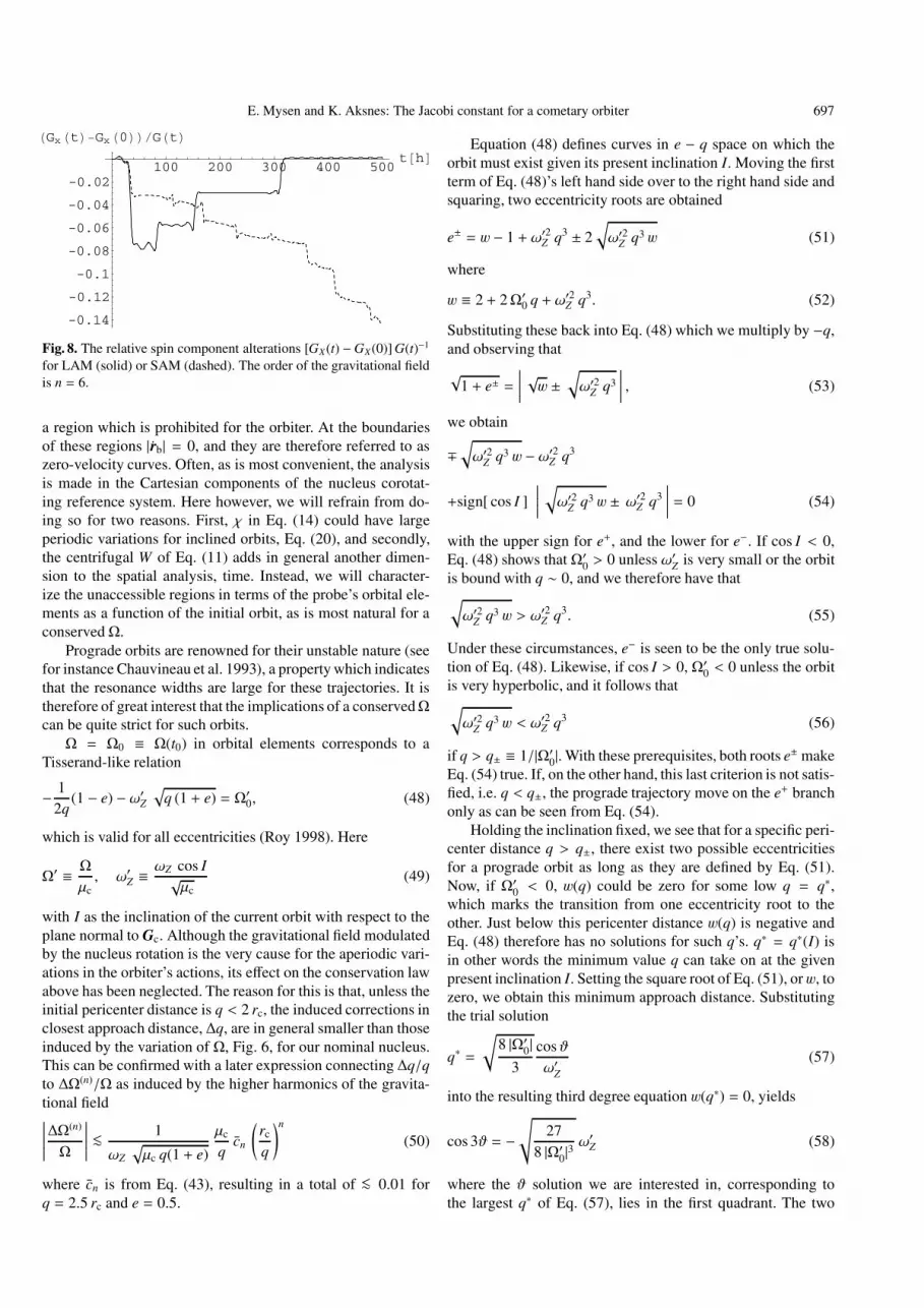
Fig. 8. The relative spin component alterations [GX(t) −GX(0)] G(t)−1

for LAM (solid) or SAM (dashed). The order of the gravitational fieldis n = 6.

a region which is prohibited for the orbiter. At the boundariesof these regions |rb| = 0, and they are therefore referred to aszero-velocity curves. Often, as is most convenient, the analysisis made in the Cartesian components of the nucleus corotat-ing reference system. Here however, we will refrain from do-ing so for two reasons. First, χ in Eq. (14) could have largeperiodic variations for inclined orbits, Eq. (20), and secondly,the centrifugal W of Eq. (11) adds in general another dimen-sion to the spatial analysis, time. Instead, we will character-ize the unaccessible regions in terms of the probe’s orbital ele-ments as a function of the initial orbit, as is most natural for aconservedΩ.

Prograde orbits are renowned for their unstable nature (seefor instance Chauvineau et al. 1993), a property which indicatesthat the resonance widths are large for these trajectories. It istherefore of great interest that the implications of a conservedΩcan be quite strict for such orbits.Ω = Ω0 ≡ Ω(t0) in orbital elements corresponds to a

Tisserand-like relation

− 12q

(1 − e) − ω′Z√

q (1 + e) = Ω′0, (48)

which is valid for all eccentricities (Roy 1998). Here

Ω′ ≡ Ωµc, ω′Z ≡

ωZ cos I√µc

(49)

with I as the inclination of the current orbit with respect to theplane normal to Gc. Although the gravitational field modulatedby the nucleus rotation is the very cause for the aperiodic vari-ations in the orbiter’s actions, its effect on the conservation lawabove has been neglected. The reason for this is that, unless theinitial pericenter distance is q < 2 rc, the induced corrections inclosest approach distance, ∆q, are in general smaller than thoseinduced by the variation of Ω, Fig. 6, for our nominal nucleus.This can be confirmed with a later expression connecting ∆q/qto ∆Ω(n)/Ω as induced by the higher harmonics of the gravita-tional field∣∣∣∣∣∣∆Ω(n)

Ω

∣∣∣∣∣∣ <∼1

ωZ

√µc q(1 + e)

µc

qcn

(rc

q

)n

(50)

where cn is from Eq. (43), resulting in a total of <∼ 0.01 forq = 2.5 rc and e = 0.5.

Equation (48) defines curves in e − q space on which theorbit must exist given its present inclination I. Moving the firstterm of Eq. (48)’s left hand side over to the right hand side andsquaring, two eccentricity roots are obtained

e± = w − 1 + ω′2Z q3 ± 2√ω′2Z q3 w (51)

where

w ≡ 2 + 2Ω′0 q + ω′2Z q3. (52)

Substituting these back into Eq. (48) which we multiply by −q,and observing that

√1 + e± =

∣∣∣∣∣√w ±

√ω′2Z q3

∣∣∣∣∣ , (53)

we obtain

∓√ω′2Z q3 w − ω′2Z q3

+sign[ cos I ]∣∣∣∣∣√ω′2Z q3 w ± ω′2Z q3

∣∣∣∣∣ = 0 (54)

with the upper sign for e+, and the lower for e−. If cos I < 0,Eq. (48) shows that Ω′0 > 0 unless ω′Z is very small or the orbitis bound with q ∼ 0, and we therefore have that√ω′2Z q3 w > ω′2Z q3. (55)

Under these circumstances, e− is seen to be the only true solu-tion of Eq. (48). Likewise, if cos I > 0, Ω′0 < 0 unless the orbitis very hyperbolic, and it follows that√ω′2Z q3 w < ω′2Z q3 (56)

if q > q± ≡ 1/|Ω′0|. With these prerequisites, both roots e± makeEq. (54) true. If, on the other hand, this last criterion is not satis-fied, i.e. q < q±, the prograde trajectory move on the e+ branchonly as can be seen from Eq. (54).

Holding the inclination fixed, we see that for a specific peri-center distance q > q±, there exist two possible eccentricitiesfor a prograde orbit as long as they are defined by Eq. (51).Now, if Ω′0 < 0, w(q) could be zero for some low q = q∗,which marks the transition from one eccentricity root to theother. Just below this pericenter distance w(q) is negative andEq. (48) therefore has no solutions for such q’s. q∗ = q∗(I) isin other words the minimum value q can take on at the givenpresent inclination I. Setting the square root of Eq. (51), orw, tozero, we obtain this minimum approach distance. Substitutingthe trial solution

q∗ =

√8 |Ω′0|

3cosϑω′Z

(57)

into the resulting third degree equation w(q∗) = 0, yields

cos 3ϑ = −√

278 |Ω′0|3

ω′Z (58)

where the ϑ solution we are interested in, corresponding tothe largest q∗ of Eq. (57), lies in the first quadrant. The two


0.5 1 1.5 2 2.5 3e

0.5

1

1.5

2

2.5

3q rc

I0Π4

I00

I00

eI0

eI0

eI0

eI0

qI0

Fig. 9. Limiting contours for two prograde orbits.

other solutions are obtained by adding or subtracting 120 fromthis ϑ.

Clearly, a probe for which this scenario holds will nevercome closer to the comet nucleus than q∗I=0 since I = 0 repre-sents the smallest minimum, corresponding to a scenario wherethe probe’s orbit is perturbed in to the nucleus’ spin plane froman initial inclination by a series of chaotic interactions. The ex-ception here is when the solution type (57) no longer exists forall inclinations; i.e. when | cos 3ϑ| > 1 at I = 0 or equivalently

|Ω′0| <32ω′2/3Z,I=0 (59)

and, as can be reasoned, the only q value which makes w(q)zero is negative. That is, if Eq. (59) is true, the conservationofΩ alone cannot guarantee that the probe avoids collision withthe nucleus for some end orbit lying close to the comet’s spinplane. However, this scenario is circumvented if the probe or-bit’s initial inclination I0 is chosen to be sufficiently low so thatEq. (59) is false. From the properties of w(q), it can be shownthat the q∗ solution we are interested in is always larger than q±for at least as long as Eq. (59) is false.

All these aspects are illustrated in Fig. 9, showing the so-lutions of Eq. (48) at I = 0 for two different orbit initial con-ditions and a nominal nucleus with Jc = 0. The solid curvesrepresent the choice I0 ≡ I(t0) = 0, in this case violatingEq. (59), while the dashed segment is produced by an initialtrajectory with I0 = π/4 and Eq. (59) being true. Both have theinitial q0 = 2.5 rc and e0 = 0.5. Each contour in the plot hasbeen identified as one of Eq. (51)’s branches. The orbit whichstarted in the spin plane can never exist between the two solidlines, while the initially inclined trajectory can never cross intothe lower right region bounded by the dashed curve. This last

0.2 0.4 0.6 0.8 1 1.2e

0.5

1

1.5

2

2.5

3

3.5

4q rc

I0Π

I03Π4

eIΠ

eIΠ

Fig. 10. Curves which mark the boundaries of the forbidden regions,lower left, for two retrograde orbits with different initial inclinationswith respect to the spin plane.

conclusion rests on the fact that e+(q) close to e = 1 (q = 0)goes as

e+(q) ≈ 1 + 2Ω′0 q + 2√

2ω′2Z q3, Ω′0 < 0 , (60)

and therefore decreases less rapidly from e = 1 with increas-ing q for a low inclination than for a large one, only to returnto a lower

qh ≡ q(e = 1) =12

(Ω′0ω′Z

)2

· (61)

e−I=0 for the initially inclined case exists if q > q±, but is notincluded since it is negative. Also, at low q’s, the irregularitiesof the gravitational field cannot be neglected, but the solutionsfor spherical symmetric gravitation are still used for solutionidentification purposes.

Likewise, the solutions of Eq. (48) at I = π for two ret-rograde orbits with different initial inclinations are shown inFig. 10. The dashed curve, marking the lower left region whichis forbidden for the probe’s orbit, represents the inclined I0 =

3π/4, as the solid line represents the boundary for the I0 = πcase. Other initial orbital parameters are as before. That the re-gion in question is forbidden follows from the fact that e−(q)close to e = 1 (q = 0) goes as

e−(q) ≈ 1 + 2Ω′0 q − 2√

2ω′2Z q3, Ω′0 > 0 , (62)

and therefore increases less rapidly from e = 1 with increas-ing q for a large | cos I| than for a small one, only to return to alower qh, Eq. (61).

Since retrograde trajectories have Ω′0 > 0, except for somespecial cases, w(q) cannot be zero in the physical range of q’s,


1 2 3 4 5r rc

-3.5

-2.5

-2

-1.5

-1

Ur rc2 h2

rs

Fig. 11. The effective potential U to zero order in the spin plane.

and there exists no minimum threshold on pericenter distancebased on a constant Ω. However, note that for the initially ret-rograde case I0 = π, the orbiting spacecraft’s orbit must changeinto a hyperbolic trajectory above a distance qh on its inboundleg if it is to collide with the nucleus. Therefore, proper precau-tions can be taken by choosing qh to be larger than the largestdistance for which such a change is thought possible. It shouldbe mentioned that retrograde orbits are as renowned for theirnon-resonant stability as the prograde are for their unstable be-haviour. Based on a large number of simulations of probes indifferent orbits around a selection of Gaussian shapes, we seethat this property also holds for excited rotation of the centralbody. This property indicates that the resonances of these tra-jectories are narrow.

In Scheeres et al. (1996), a similar analysis like the oneabove has been presented where the Jacobi integral’s conse-quences were studied. In addition to representing solutions forgeneral inclinations implied by such a conserved quantity, wehave here also explicitly determined their regions of applica-bility. If we for the moment restrict our attention to uniaxialrotation, Scheeres et al. (1996) used the Jacobi integral to deter-mine whether or not an orbiting particle could have emanatedfrom the central body. That is, if the particle’s χ is smaller thanthe value of the effective potential U = V +W, Eq. (14), eval-uated at the central body’s surface, it follows that r2

b for theparticle is negative there.

A graphical presentation of this is included as Fig. 11, aplot of U(r), for simplicity set to U = V0 +W, in the spin planefor our nominal nucleus parameters. The function peaks at thesynchronous orbit

rs =

µc

ω2Z

1/3

(63)

which, unless the central body has some cohesion, is alwayslarger than the largest physical dimension of the body in thespin plane, for convenience denoted rc. In such a circumstance,χ(r, rb = 0) = U(r) = U(rc) has two r solutions, one at rc, andanother one a distance beyond rs. Clearly, there exist a series oforbits with U(rs) > χ(r > rs) > U(rc) which do not originatefrom the central body either, and the criterion of Scheeres et al.(1996) is therefore, in a way, too strict. This nuance is howeveraccounted for by Eqs. (57) and (59) which in the spin planereduces to what we have discussed above.

In general, particles in a prograde orbit do not come from,or an orbiter does not collide with the central body if Eq. (59) is

0.5 1 1.5 2 2.5 3e

0.5

1

1.5

2

2.5

3

3.5

4q rc

Fig. 12. Limiting contour (solid) for an I0 = 0, e0 = 0.5, q0 = 2.5 rc

orbit in the nucleus spin plane, I = 0. The dashed curves represent thedisplaced limiting contours if Ω is increased or decreased slightly.

false, |χ| > |U(rs)| in the spin plane for one-axis rotation, and ifq0 > q∗I=0 > rc, corresponding to r0 > rs > rc in the spin planefor the restricted problem. The lower left e+I=0 branch of Fig. 9represents the pocket of bound trajectories with |χ| > |U(rs)|and r0 < rs, see Fig. 11.

5. Non-gravitational and tidal forcesShortly after comet rendezvous, the small module Philae willbe separated from Rosetta so that it can land on 67P’s nu-cleus. Although close prograde orbits undergo large and rapidchanges in their parameters, they are attractive (Bertrand et al.2004) for this particular phase; the relative speed between thelander and the nucleus is minimized so that Philae is not, forinstance, buried beneath the comet surface (Kührt et al. 1997).This is made even more relevant by the fact that the lander wasconstructed for the probably lighter 46P/Wirtanen, as can be in-ferred from a comparison of the comet’s perihelion water pro-duction rate and observed non-gravitational displacements ofits orbit.

We have argued that, as long as certain precautions are met,Rosetta is unlikely to collide with the nucleus under the actionof gravitation alone during such a maneuver. However, also toanswer issues of impact avoidance on time-scales which stretchover several orbits, the rate at which solar radiation and out-gassing pressure changes Ω must be addressed. The situationhere is quite different from NEAR’s retrograde landing on Eroswhich is almost thousand times more massive (Miller et al.2002) than our nominal comet nucleus.

Before proceeding, we include a plot which illustrates howsensitive the minimum pericenter distance is for variationsinΩ. The situation in Fig. 12 is identical to one of the two orbitsplotted in Fig. 9. This time however, the limiting contours forthe cases whereΩ0 of Eq. (48) is changed with ∆Ω0 = ±0.05Ω,


with Ω equal to the value at the solid curve, are also added. Wesee that small variations in the modified Jacobi function inducefairly small relative variations in minimum q. A more conve-nient expression for the corresponding change in pericenter dis-tance can be conjured by differentiating Eq. (61), resulting in

∆qh

qh= 2∆Ω

Ω· (64)

5.1. Outgassing pressure

At the time when the lander is delivered, somewhere beyondthe comet heliocentric distance of R = 3−4 AU, the sublimationof water from the nucleus is negligible (Crifo et al. 1999), butoutgassing of more volatile species like CO, less modulatedby R (Capria et al. 2004), could be significant.

With f as the perturbing force per mass unit, it follows fromEqs. (9) and (13) that the Jacobi function’s associated rate ofchange obeys

χ = Ω = f · rb. (65)

Following Montenbruck & Gill (2000), the pressure force onthe orbiting spacecraft per mass unit exerted by the outflowingmolecules of the coma is f c = AS/C ρ v u/mS/C (the drag coef-ficient CD is here set to two), where ρ is the mass density ofthe coma, u the relative velocity between probe and flow, andat last mS/C and AS/C are the spacecraft’s mass and its gas ex-posed area, respectively. If not very close to the nucleus, wherethe flow could be almost along the comet surface (Crifo et al.1995), u/v = r/r is a common assumption. This is related to thefact that while the cometocentric velocity of a probe in a boundorbit is ∼0.1 m s−1, the velocity of the collisionally acceleratedoutflowing molecules could typically be as high as ∼1 km s−1

(Crifo & Rodionov 1997).Writing f c = Λ(r) r/r3, it has been shown, based on simu-

lations of some cometary comae (Scheeres et al. 2000), that Λis approximately dependent on direction only, and not on dis-tance. That is, if φ and θ are cometocentric direction angles,Λ(r, φ, θ) ≈ Λ(φ, θ). In particular, this dependency reappearsin the simulations of 67P/Churyumov-Gerasimenko’s coma byCrifo et al. (2004) in the solar direction where the pressure isstrongest. A CO rate of 1027 mol. s−1, a worst-case scenario(Bockelée-Morvan et al. 2004), seems (Crifo et al. 2004) toyield an approximate maximum ΛM = 0.1 r3

c h−2 for full expo-sure of the solar cell arrays. rc here has nothing to do with thenucleus directly, but is just our prefered unit of length.

The outgassing induced change of Ω on an inbound legfrom apocenter p at time tp, to pericenter q at time tq, can theneasily be evaluated

∆Ωc =

∫ tq

tp

dtΛ

r3r · rb =

∫ tp

tq

dtΛddt

1r= Λ

(1p− 1

q

)(66)

which amounts to only a few percent of Ω0 even if the angularmean Λ is set to ΛM, and the pericenter distance is a very closeq = 2 rc.

More interestingly, Ω decreases on the probe’s journey to-wards the nucleus. And since impact avoidance of a probe ina prograde orbit is achieved by minimizing Ω, i.e. maximizing

its absolute value, Eq. (59), outgassing will actually make suchan orbit safer from a dynamical point of view. For a retrogradeorbit, the opposite occurs because large positive Ω’s are morefavourable, Eq. (61), making an inbound orbit more hazardousunder the influence of outgassing pressure.

5.2. Solar radiation pressure

If all incident photons are absorbed by Rosetta’s large solar cellarrays, composed of specially developed non-reflective silliconcells, the induced force per mass unit acting on the spacecraftcan be written

f = − ΘR2

u, Θ = 0.001 rc h−2. (67)

R is as before the comet’s heliocentric distance and u a come-tocentric unit vector in the direction of the Sun. Θ is a strengthparameter equal to the given high value for maximum area ex-posure to solar radiation, and if R is dimensionless and evalu-ated in astronomical units.

It is straightforward to show that the radiation pressure in-duced acceleration can be derived from a potential V = − f·r,but the effect cannot be included by merely adding this poten-tial to the Jacobi function. This is due to the potential’s explicitdependency on time, see Eq. (13), which changes Ω at a rela-tively rapid pace. Therefore, a direct approach is more advis-able. Using Eq. (65) we have

∆Ω = − ΘR2

∫ t

t0

dt [ u · r − u · (ω × r) ] , (68)

where the second of the bracketed terms is of most interestsince its maximum is dominant at distances above the syn-chronous radius a = 1.6 rc for the adopted rotation period,Table 2.

On one leg of an orbit, the radiation pressure in-duced change of the Jacobi function is hence approximatelybounded by

|∆Ω| < ΘR2

ωZ

G

∫ 0

−πd f r3 =

Θ

R2

ωZ√µc

a5/2 π

(1 +

12

e2

)(69)

with the use of the relation dt = d f r2/G. The relative alter-ation is

∣∣∣∣∣∆ΩΩ

∣∣∣∣∣ <Θ

R2

π

µc

1 + 1/2 e2

√1 − e2

a2, (70)

which again amounts to only a few percent for the probe inan eccentric a = 5 rc orbit at R = 3 AU. However, due to thequadratic semi-major axis dependency of Eq. (70), more distantorbits could accumulate non-negligible changes in Ω. Thesecan, on the other hand, be reduced with a proper choice of or-bital geometry, minimizing the integrated part of Eq. (68). Ifthe solar cell arrays do not rotate relative to the direction of theSun, the secular problem is solvable (Mignard & Henon 1984)in terms of the heliocentric distance R, i.e. the induced changesof the orbit are slow.


5.3. Tidal acceleration

An orbiting spacecraft is also affected by the gravitational pullfrom the Sun which, if described relative to the comet, is coun-tered by an effective acceleration equal in magnitude to theheliocentric acceleration of the nucleus. Although the highlyelliptic orbit of the nucleus does not make it clear that suchconcepts can be used, the effect of the solar tidal accelerationcan nevertheless be gauged by calculating the “capture radius”of this isolated problem. The radius of the Hill sphere (Murray& Dermott 1999) is

rH = R

(µc

3 µ

)1/3

= 270 rc (71)

where the tabulated value is at comet heliocentric distance R =3 AU. At the same R, the solar radiation pressure accelerationequals the zero-order gravitational pull from the nucleus at r =100 rc. Of course, solar radiation pressure will strip the probefrom the comet below this distance. That is, tidal accelerationis negligible for the applications in this paper.

6. Conclusions

For a probe under the gravitational attraction of a uniformlyrotating irregular central body, there exists an integral of mo-tion called the Jacobi constant. If its implications are to be ofrelevance to the Rosetta mission a priori, one must investigatewhat happens to this function if the target comet’s rotation isnot uniaxial.

We have argued that there exists a Tisserand-like quantity,identical to the Jacobi constant for non-excited rotation, whichis sufficiently conserved in general for it to have interestingimplications for the evolution of the probe’s orbit. In particular,its near constancy can be used to design close prograde orbitswhich under the action of gravitation alone do not evolve intocollision trajectories with the comet nucleus. These orbits arerelevant for the lander delivery phase of the Rosetta missiondespite their notoriously unstable nature.

An analysis based solely on the Tisserand-like quantity’sconservation shows that impact is best avoided if the probe’sinitial orbit is chosen to be retrograde or prograde with its ini-tial cometocentric velocity lying in the plane normal to the nu-cleus spin. Non-gravitational forces are, for our chosen nomi-nal nucleus at heliocentric distance 3−4 AU, not seen to changethe pseudo-integral enough to affect the above conclusions ina worst-case scenario. More specifically, the adopted radialoutgassing pressure makes the unstable close prograde orbitsslightly safer, while close retrograde trajectories become some-what more hazardous.

Acknowledgements. This work was done as a part of project153382/V30, The Research Council of Norway.

References

Beletskii, V. V. 1966, Motion of an Artificial Satellite About Its Centerof Mass, Mechanics of Space Flight Series, Israel Program forScientific Translations, Jerusalem

Bertrand, R., Ceolin, T., & Gaudon, P. 2004, Rosetta LanderDescending Phase on the Comet 67P/Churyumov-Gerasimenko,18th International Symposium on Space Flight Mechanics

Bockelée-Morvan, D., Moreno, R., Biver, N., et al. 2004, in The NewROSETTA Targets, ed. L. Colangeli, E.M. Epifani, & P. Palumbo,(Dordrecht: Kluwer), ASSL, 311, 25

Byrd, P. F., & Friedman, M. D. 1971, Handbook of Elliptic Integralsfor Engineers and Scientists (Berlin: Springer-Verlag)

Capria, M. T., Coradini, A., De Sanctis, M. C., et al. 2004, in The NewROSETTA Targets, ed. L. Colangeli, E. M. Epifani, & P. Palumbo,(Dordrecht: Kluwer), ASSL, 311, 177

Chauvineau, B., Farinella, P., & Mignard, F. 1993, Icarus, 105,370

Crifo, J. F., & Rodionov, A. V. 1997, Icarus, 127, 319Crifo, J. F., Itkin, A. L., & Rodionov, A. V. 1995, Icarus, 116, 77Crifo, J. F., Rodionov, A. V., & Bockelée-Morvan, D. 1999, Icarus,

138, 85Crifo, J. F., Lukyanov, G. A., Zakharov, V. V., et al. 2004, in The New

ROSETTA Targets, ed. L. Colangeli, E. M. Epifani, & P. Palumbo,(Dordrecht: Kluwer), ASSL, 311, 119,

Davidsson, B. J. R, & Gutiérrez, P. J. 2005, Icarus, 176, 453Garmier, R., & Barriot, J.-P. 2001, Cel. Mech., 79, 235Goldstein, H. 1980, Classical Mechanics, Addison-Wesley, ReadingGutiérrez, P. J., Jorda, L., Samarasinha, N. H., et al. 2003, Outgassing-

induced effects in the rotational state of comet 67P/Churyumov-Gerasimenko during the Rosetta mission, DPS 35th Meeting

Heiskanen, W. A., & Moritz, H. 1967, Physical Geodesy (SanFrancisco: W.H. Freeman and Company)

Hitzl, D. L., & Breakwell, J. V. 1971, Cel. Mech., 3, 346Kinoshita, H. 1972, PASJ, 24, 423Kührt, E., Knollenberg, J., & Keller, H. U. 1997, Planet. Space Sci.,

45, 665Lamy, P. L., Toth, I., Weaver, H., et al. 2003, The Nucleus of Comet

67P/Churyumov-Gerasimenko, the New Target of the RosettaMission, DPS 35th Meeting

Lichtenberg, A. J., & Lieberman, M. A. 1992, Regular and ChaoticDynamics (New York: Springer-Verlag)

Mignard, F., & Henon, M. 1984, Cel. Mech., 33, 239Miller, J. K., Konopliv, A. S., Antreasian, P. G., et al. 2002, Icarus,

155, 3Montenbruck, O., & Gill, E. 2000, Satellite Orbits (Germany:

Springer-Verlag)Muinonen, K. 1998, A&A, 332, 1087Muinonen, K., & Lagerros, J. S. V. 1998, A&A, 333, 753Murray, C. D., & Dermott, S. F. 1999, Solar System Dynamics

(Cambridge: Cambridge University Press)Mysen, E. 2004, Planet. Space Sci., 52, 897Rickman, H., Kamél, L., Festou, M. C., et al. 1987, ESA SP-278,

471Rossi, A., Marzari, F., & Farinella, P. 1999, Earth, Planets Space, 51,

1173Roy, A. E. 1998, Orbital Motion (Bristol: Institute of Physics

Publishing)Scheeres, D. J., Ostro, S. J., Hudson, R. S., et al. 1996, Icarus, 121,

67Scheeres, D. J., Bhargava, S., & Enzian, A. 2000, TMO Progress Rep.,

42

Documents

The Jacobi constant for a cometary orbiter